the Creative Commons Attribution 4.0 License.
the Creative Commons Attribution 4.0 License.
 | 28 Sep 2022
Impact of urbanization on gas-phase pollutant concentrations: a regional-scale, model-based analysis of the contributing factors
Jan Karlický
Lukáš Bartík
Marina Liaskoni
Alvaro Patricio Prieto Perez
Kateřina Šindelářová
Urbanization or rural–urban transformation (RUT) represents one of the most important anthropogenic modifications of land use. To account for the impact of such process on air quality, multiple aspects of how this transformation impacts the air have to be accounted for. Here we present a regional-scale numerical model (regional climate models RegCM and WRF coupled to chemistry transport model CAMx) study for present-day conditions (2015–2016) focusing on a range of central European cities and quantify the individual and combined impact of four potential contributors. Apart from the two most studied impacts, i.e., urban emissions and the urban canopy meteorological forcing (UCMF, i.e., the impact of modified meteorological conditions), we also focus on two less studied contributors to the RUT impact on air quality: the impact of modified dry deposition due to transformed land use and the impact of modified biogenic emissions due to urbanization-induced vegetation modifications and changes in meteorological conditions affecting these emissions. To quantify each of these RUT contributors, we performed a cascade of simulations with CAMx driven with both RegCM and WRF wherein each effect was added one by one while we focused on gas-phase key pollutants: nitrogen, sulfur dioxide (NO2 and SO2), and ozone (O3).
The validation of the results using surface observations showed an acceptable match between the modeled and observed annual cycles of monthly pollutant concentrations for NO2 and O3, while some discrepancies in the shape of the annual cycle were identified for some of the cities for SO2, pointing to incorrect representation of the annual emission cycle in the emissions model used. The diurnal cycle of ozone was reasonably captured by the model.
We showed with an ensemble of 19 central European cities that the strongest contributors to the impact of RUT on urban air quality are the urban emissions themselves, resulting in increased concentrations for nitrogen (by 5–7 ppbv on average) and sulfur dioxide (by about 0.5–1 ppbv) as well as decreases for ozone (by about 2 ppbv). The other strongest contributor is the urban canopy meteorological forcing, resulting in decreases in primary pollutants (by about 2 ppbv for NO2 and 0.2 ppbv for SO2) and increases in ozone (by about 2 ppbv). Our results showed that they have to be accounted for simultaneously as the impact of urban emissions without considering UCMF can lead to overestimation of the emission impact. Additionally, we quantified two weaker contributors: the effect of modified land use on dry deposition and the effect of modified biogenic emissions. Due to modified dry deposition, summer (winter) NO2 increases (decreases) by 0.05 (0.02) ppbv, while there is almost no average effect for SO2 in summer and a 0.04 ppbv decrease in winter is modeled. The impact on ozone is much stronger and reaches a 1.5 ppbv increase on average. Due to modified biogenic emissions, a negligible effect on SO2 and winter NO2 is modeled, while for summer NO2, an increase by about 0.01 ppbv is calculated. For ozone, we found a much larger decreases of 0.5–1 ppbv.
In summary, when analyzing the overall impact of urbanization on air pollution for ozone, the four contributors have the same order of magnitude and none of them should be neglected. For NO2 and SO2, the contributions of land-use-induced modifications of dry deposition and modified biogenic emissions have a smaller effect by at least 1 order of magnitude, and the error will thus be small if they are neglected.
- Article
(14605 KB) - Full-text XML
- BibTeX
- EndNote


Urbanization represents one of the most important transformations of land use, turning the natural surface into a built-up surface with objects like buildings, streets, and roads. While urban areas only represent less than 1 % a percent of the total Earth surface (Gao and O'Neill, 2020), more than half of the Earth's population already lives in cities (UN, 2018a), and this transformation, which is often called rural–urban transformation (RUT), is still an ongoing process. It is expected that in the upcoming decades, more than 60 % of the population will live in urban areas (UN, 2018b), making research focused on their environmental effects more and more crucial.
It is known that urban areas predominantly affect the atmospheric environment (Folberth et al., 2015), and they act via two primary intrusions that urbanization represents within the natural environment: (i) the introduction of urban land surface replacing rural land surface, causing significant modifications of the meteorological conditions (Oke et al., 2017) and climate (Huszar et al., 2014; Zhao et al., 2017), and (ii) the introduction of a massive emissions source of anthropogenic pollutants perturbing not only local but also regional and global air composition (Lawrence et al., 2007; Timothy and Lawrence, 2009; Im and Kanakidou, 2012; Huszar et al., 2016a).
As for the air quality of urban areas and those surrounding large cities, it is clear that the main driver affecting the concentrations are local urban emissions. Indeed, many studies looked at the perturbation of the atmospheric composition due to solely urban emissions over different scales. For example, Lawrence et al. (2007), Butler and Lawrence (2009), and Stock et al. (2013) investigated the global impact of emissions from megacities, while on regional scales many studies focused on large agglomerations in Europe, like Athens, Istanbul, London, and Paris (e.g., Im et al., 2011a, b; Im and Kanakidou, 2012; Finardi et al., 2014; Skyllakou et al., 2014; Markakis et al., 2015; Hodneborg et al., 2011; Huszar et al., 2016a; Hood et al., 2018), or on large eastern Asian pollution hot spots (Guttikunda et al., 2003, 2005; Tie et al., 2013). These studies show that, not surprisingly, the concentrations of primary pollutants like oxides of nitrogen and sulfur (NOx, SO2), volatile organic compounds, and primary aerosols are substantially increased. But on the other hand, urban emissions, due to their high NOx-to-VOC ratio (VOC: volatile organic compound), can lead to decreases in ozone in the urban cores (e.g., Huszar et al., 2016a). There is further a general consensus in these studies that although air pollution in cities is determined mainly by local sources, a significant fraction of the total concentration is associated with rural sources or sources from other cities (Panagi et al., 2020; Thunis et al., 2021; Huszar et al., 2021).
Urbanization, however, influences the final air pollution in other ways too. One of the most studied aspects of RUT is the modulation of the pollutant concentration due to the meteorological forcing represented by the urban canopy, which includes effects like increased temperatures (urban heat island, UHI) (Oke, 1982; Oke et al., 2017; Karlický et al., 2018, 2020; Sokhi et al., 2022), lower wind speeds (Jacobson et al., 2015; Zha et al., 2019), or elevated boundary layer height along with enhanced vertical eddy diffusion (Ren et al., 2019; Huszar et al., 2020a; M. Wang et al., 2021). Huszar et al. (2020a) introduced the term urban canopy meteorological forcing (UCMF), which represents the forcing that the land surface modified by RUT represents for the physical state of the air above via perturbed exchange of momentum, heat, radiation, and moisture. UCMF is thus a modification of meteorological conditions, which in turn propagates to modifications of pollutant concentrations via modifying the transport, chemical transformation, and deposition of air pollutants. Indeed, Ulpiani (2021) argued that urban pollution has to be studied in connection with UHI and other related meteorological effects. Many other studies looked at the impact of UCMF on air quality and found that the most important parameters in this regard are temperature, turbulence, and wind (Struzewska and Kaminski, 2012; Liao et al., 2014; Kim et al., 2015; Zhu et al., 2017; Zhong et al., 2018; Li et al., 2019; Huszar et al., 2014, 2018a, 2020b), while moisture effects were rather minor (Huszar et al., 2018b). These studies found that these changes led to near-surface decreases in primary pollutant concentrations, while in the case of secondary pollutants (e.g., ozone) increases are encountered either on the surface or at higher levels (Huszar et al., 2018a; Janssen et al., 2017; Yim et al., 2019; Li et al., 2019; Kim et al., 2021; Kang et al., 2022). In other words, besides the urban emission input, UCMF is another factor that contributes to the final urban pollution within the overall process of RUT (Huszar et al., 2021).
Moreover, during urbanization the land use is modified from rural (or natural like forest and grassland) to “urban”, which itself introduces a forcing via a further pathway: contrary to wet deposition, dry deposition velocities (DVs) greatly depend on the land use type, which determines the resistance of the surface and canopy layer (Zhang et al., 2003; Cherin et al., 2015; Hardacre et al., 2021). In urban environments, vegetation is greatly reduced (expressed, for example, in terms of the leaf area index – LAI – reduction). As plants represent a major sink for many gaseous air pollutants (via stomatal uptake), it is clear that over urban areas, this sink is missing or is strongly reduced. For example, based on a later study, over urban land surface the typical DVs of nitrogen dioxide (NO2) and ozone (O3) are about half of that above agricultural land like crops (as a typical rural land surface type). Nowak and Dwyer (2007) calculated a net average pollutant removal if additional trees were planted in select US urban areas. Mcdonald-Buller et al. (2001) also showed that ozone and NO2 are greater in a photochemical model if the land use information supplied contains a higher fraction of urban land use type. In general it seems that, besides other effects, urbanization also leads to increased ozone concentrations due to reduced deposition values (Song et al., 2008; Tao et al., 2015), while dry deposition itself is an important factor determining ozone pollution (Galmarini et al., 2021). However, for some secondary pollutants like HNO3, H2SO4, H2O2, HONO, or NH3, the removal in the case of wet canopies is higher for urban areas than for rural ones (e.g., crops) due to their high solubility and reactivity with solid surfaces (Zhang et al., 2003). Urbanization in the case of these species means higher DVs, leading to a decrease in their concentrations. It is thus clear that the final air pollution caused by urbanization has another contribution represented by the modified (increases and decreases too) dry deposition uptake potential of urban land surface compared to rural and/or natural land surface.
Finally, vegetation not only acts as a sink of pollutants via dry deposition, but it also emits large quantities of biogenic hydrocarbons (biogenic volatile organic compounds – BVOCs; Kesselmeier and Staudt, 1999). Due to their reactivity and potential to form peroxy radicals, they contribute to the formation of tropospheric ozone (Situ et al., 2013; Tagaris et al., 2014). As already mentioned above, during urbanization, the vegetation is strongly reduced, which will result in a decrease in BVOC emissions. Song et al. (2008), for example, showed up to 10 % reductions due to urbanization in Texas. As urban areas are usually VOC-limited environments, reduced BVOC emissions are expected to lead to reduced ozone concentrations (Song et al., 2008). It has to be noted that anthropogenic emissions from urban areas encompass the emissions of VOC compounds, typically of biogenic origin (like isoprene and monoterpenes; Wagner and Kuttler, 2014; Panopoulou et al., 2020). These emissions are probably much smaller than other VOC emissions (Guo et al., 2022) and cannot outweigh the reduction due to reduced vegetation.
Urbanization-induced BVOC emission modifications have a further sub-component acting via modified meteorological conditions in cities. Indeed, urban temperatures are higher than rural ones, and there is an indication that urban cloudiness, at least for European cities, is slightly reduced too (Karlický et al., 2020). These effects have a direct impact on the biochemistry of plants and thus on the quantity of emitted BVOCs as higher temperatures and more solar radiation promote these emissions (Guenther et al., 2006). This means that, due to urbanization, BVOC emissions are suppressed by reducing the vegetation fraction; however, more favorable weather conditions act in an opposite way, making these effects counteracting, although there is an indication that the former (vegetation) effect is dominant (Li et al., 2019).
In summary, urbanization substantially affects air quality, while the final urban pollutant concentration levels are a result of multiple impacts that add to the background (i.e., that without urbanization) air pollution. These include the following.
-
The effect of urban emissions (DEMIS)
-
The effect of the urban canopy meteorological forcing (UCMF) on pollutant transport and chemistry (DMET)
-
The effect of modified dry deposition associated with modified land cover (DLU_D)
-
The effect of modified emissions of biogenic volatile compounds (BVOCs) due to modified land cover (i) and meteorology (ii) (DBVOC)
As seen above, many studies looked at the total impact of urbanization or at some of the individual contributors listed. However, they did not systematically analyze the impact of each one of them. Here we propose a study to uncover the (i) total impact of urbanization (DTOT) and, more importantly, the contribution of (ii) each of the urbanization-related impacts (i.e., DEMIS, DMET, DLU_D, and DBVOC) over a regional-scale domain to present-day urban air pollution levels using coupled regional climate and chemistry transport models applied at moderate 9 km × 9 km horizontal resolution. To achieve this goal, we have to define the reference (or background; not to be confused with “background ozone”, which is a well-defined term) state to which these impacts will be gradually added: rural land use without the effect of UCMF and only rural emissions (urban emissions removed, i.e., those falling within the city administrative boundaries), while present-day land use, emissions, and climate are considered (2015–2016, see below). To evaluate the individual contributors to urbanization as well as their combined effect, we will gradually add each of them to the base simulation in a cascading fashion. To reduce the uncertainty of the results caused by the different geographical and climatic conditions of cities, we perform our analysis for a large ensemble of cities in central Europe: 19 cities in total. Although a similar estimate across several urban areas was made in Huszar et al. (2016a), they focused on the effect of emissions only (which corresponds to DEMIS in our study), while none of the other effects (UCMF; effect of land use on dry deposition and effect of modified biogenic emissions) were considered. Further, it is clear that to some degree the urbanization of one geographic location will affect the air pollution of other urban areas; however, this effect was evaluated to be minor for emissions and UCMF if the cities analyzed are sufficiently far from each other (Huszar et al., 2014, 2016a). Therefore, the selection of cities considers the requirement of sufficient distance from each other.
The study will focus on the key gas-phase pollutants NO2, O3, and SO2. NO2 is one of the most important primary pollutants in urban environments responsible for reduced air quality and as a precursor for secondary pollutants like ozone or inorganic fine aerosol (Im and Kanakidou, 2012; Stock et al., 2013; Mertens et al., 2020). Ozone is formed in urban plumes when NOx and VOCs mix together promoted by solar radiation (Xue et al., 2014). Finally, sulfur dioxide is a pollutant originating mainly from fossil fuel combustion in energy production (Guttikunda et al., 2003); although it has undergone significant reduction in European cities during the last decades, it remains of concern, especially in eastern European countries (e.g., in Poland; EEA, 2019).
Of course, urban air pollution is affected not only by local effects. Emissions from other areas (rural or other, even distant cities) constitute a major fraction of urban air pollution (Im and Kanakidou, 2012; Huszar et al., 2016a). Further, background regional air pollution is an important factor that plays a role, e.g., in the urban ozone burden (Yan et al., 2021). Also, UCMF can have regional effects, and the UCMF due to one city can have an effect others (Huszar et al., 2014). However, in this study we are interested in the local effects, i.e., the effect of rural–urban transformation on the local final air pollution, and concerned about the effect of the background atmosphere or the effect from other urban areas.
The study is structured as follows: after the Introduction, the experimental tools (models), their configuration, and the data used are presented. Next, the experiments performed are presented, followed by the Results section. Finally, these aspects are discussed and conclusions are drawn.
2.1 Models used
The study is based on numerical experiments carried out using regional climate models (RCM) coupled to a chemistry transport model (CTM). To describe the regional climate, two RCMs as meteorological driver are used: RegCM version 4.7 and WRF version 4.0.3. Chemistry was resolved with the chemical transport model CAMx in version 7.10. The decision behind choosing two regional meteorological drivers is to achieve, at least to some degree, more robust results given the fact that the modeled meteorological conditions over cities greatly impacts the chemical concentrations (Ďoubalová et al., 2020; Huszar et al., 2018b).
As the models used and the parameterizations applied are almost identical to those in Huszar et al. (2021), here we list the most important details. RegCM4.7 is a regional-scale climate model with both hydrostatic and non-hydrostatic dynamics (Giorgi et al., 2012). The schemes adopted are the Tiedtke scheme (Tiedtke, 1989) for convection, the Holtslag scheme (HOL; Holtslag et al., 1990) for planetary boundary layer (PBL) parameterization, and the five-class WSM5 moisture scheme (Hong et al., 2004) for microphysics. The atmosphere–biosphere–surface exchange in RegCM was calculated using the Community Land Model (CLM) version 4.5 (Oleson et al., 2013) land surface scheme, and to resolve the urban-scale meteorological phenomena the CLMU module within CLM4.5 is invoked (Oleson et al., 2008, 2010). CLMU considers the traditional canyon geometry approach, meaning that cities are represented as networks of street canyons with specified geometrical and surface parameters (Oke et al., 2017).
WRF (Weather Research and Forecasting Model) is a regional weather prediction and climate model with a detailed description provided by Skamarock et al. (2019). In our modeling setup, the Grell 3D convection scheme (Grell, 1993), the BouLac PBL scheme (Bougeault and Lacarrère, 1989), and the Purdue Lin scheme (Chen and Sun, 2002, PLIN) for microphysics were used. The urban canopy meteorological effects were resolved using the Single-Layer Urban Canopy Model (SLUCM; Kusaka et al., 2001).
For the chemistry simulations the chemistry transport model CAMx version 7.10 (Ramboll, 2020) was used (i.e., we used the most up-to-date version for CAMx available). CAMx is an Eulerian photochemical CTM implementing multiple gas-phase chemistry schemes (Carbon Bond 5 and 6, SAPRC07TC, etc.) with the Carbon Bond 6 revision 5 (CB6r5) scheme used in this study. CB6r5 includes updates to chemical reaction data from IUPAC (IUPAC, 2019) and NASA (Burkholder et al., 2019) for inorganic and simple organic species important for the formation of ozone. Apart from the inclusion of the CB6r5 mechanism, this version of CAMx includes important modifications of secondary aerosol formation via oxidation of VOCs, which can have feedbacks on the total VOC and thus ozone concentrations. To complete the atmospheric chemistry with aerosol physics, a static two-mode approach was considered. The ISORROPIA thermodynamic equilibrium model (Nenes et al., 1998) was invoked for the secondary inorganic aerosol formation. Secondary organic aerosol (SOA) was partitioned from its gas-phase precursors using the SOAP equilibrium scheme (Strader et al., 1999). For wet deposition, the Seinfeld and Pandis (1998) scheme is used, while dry deposition is treated using the Zhang et al. (2003) method. The Zhang method incorporates a three-resistance equation for deposition velocity (DV) incorporating the aerodynamic resistance (ra), the above-canopy quasi-laminar sublayer resistance (rb), and the overall canopy resistance (rc), while DV is calculated as the reciprocal of the sum of these resistances. An important component of rc is the resistance represented by vegetation with the so called in-canopy aerodynamic, stomatal, mesophyll, and cuticle resistances. Over urban surfaces or any other non-vegetated surfaces, these are not defined; however, to use the same equations for such land use categories in the dry deposition model, very large values are applied (e.g., 1025 sm−1). Regarding the aerodynamic resistance representing the bulk transport trough the lowest model layer via turbulent diffusion, its magnitude depends on the intensity of turbulence, which in turn depends on wind speed, surface roughness, near-surface temperature lapse rate, and solar insolation. Over urban areas these are also strongly modulated, implying a strong influence on the deposition velocities. Finally, the quasi-laminar sublayer (or boundary) resistance rb represents molecular diffusion through the thin layer of air directly in contact with the surface, and this is assumed to be a function of the molecular diffusivity of each pollutant regardless of the surface it is deposited on. In this dry deposition model, the aerodynamic resistance has a strong dependence on the temperature via decreased stability near the surface and thus more efficient turbulent diffusion towards the surface (Louis, 1979). Also, the stomatal resistance decreases with higher temperatures due to wider stomata (Zhang et al., 2002); this holds up to a threshold maximum temperature at which stomata suddenly close. These temperatures are usually, however, not reached in the climate of the region. Therefore, increased dry deposition velocities are expected as the result of increased temperatures in urban areas.
A meteorological preprocessor is used to convert the RegCM and WRF meteorological data into model-ready driving data for CAMx: for the WRF, it was the wrfcamx preprocessor, which is provided along with the CAMx code at https://www.camx.com/download/support-software/ (last access: 27 September 2022), while for RegCM, the RegCM2CAMx interface was applied (Huszar et al., 2012). The vertical eddy diffusion coefficients (Kv) are diagnosed from the available meteorological data on RegCM and WRF output using the CMAQ diagnostic approach (Byun and Ching, 1999). Temperature, pressure, humidity, and cloud–rain water content are defined at cell centers along with pollutant concentration, and CAMx considers them to be grid cell average conditions. On the other hand, wind and diffusion coefficients are carried at cell interfaces to describe the mass transfer across each cell face. Coupling between CAMx and the driving models is offline, which implies that no feedbacks of the pollutant concentrations on WRF/RegCM radiation and microphysical processes were considered. Indeed, Huszar et al. (2016b) showed with 10-year-long simulations that the long-term radiative effects of urban pollutant emissions and secondarily formed pollutants (like ozone) are rather small, which justified this choice.
2.2 Model setup and data
Model simulations were performed over identical domains (parent and nested ones) and for an identical period as in Huszar et al. (2021), i.e., the years 2015–2016 with 9, 3, and 1 km horizontal resolution centered over the Czech capital, Prague (50.075∘ N, 14.44∘ E; Lambert conic conformal projection). In the vertical, the model grid has 40 layers in both meteorological driving models. The thickness of the lowermost layer is about 30 m, and the top of the model's atmosphere reaches 5 hPa (about 36 km). The simulated time period is December 2014–December 2016 (the first month is used as spin-up). Tie et al. (2010) argued that the ratio of the diameter of the analyzed city to model resolution should be at least 6 : 1, which means that in our case, a 6 km or smaller horizontal grid step should be used to resolve the impact of urbanization for the cities chosen (see below). For Prague, which is modeled at 1 km, this is fulfilled. Other cities outside the inner 1 km nested domain are treated at coarser resolution, but many studies found that the impact of the resolution of emissions and models on urban species concentrations is rather small: e.g., Hodneborg et al. (2011) showed that coarse resolution can lead to higher ozone modeled by around 10 %, while Markakis et al. (2015) found only moderate sensitivity (8 %) to model resolution. Similarly, Y. Wang et al. (2021) showed that ozone production is reduced when high resolution is applied, but the reduction is only about 8 % for ozone.
The ERA-Interim reanalysis (Simmons et al., 2010) is used as forcing data. The 3 and 1 km domains are then driven by the corresponding parent domains with one-way nesting. Chemical boundary conditions are based on the CAM-chem global model data (Buchholz et al., 2019; Emmons et al., 2020). Land use data (for both climate models and for the dry deposition scheme in CAMx) were derived from the high-resolution (100 m) CORINE CLC 2012 land cover data (https://land.copernicus.eu/pan-european/corine-land-cover, last access: 8 August 2022) as well as from the United States Geological Survey (USGS) database for grid cells with no information from CORINE. In RegCM, fractional land use is considered, while in WRF, each grid cell is attributed the dominant land use, which brings some accounting for the uncertainty related to the urban land cover representation. This means that due to the fact that the land use is represented differently in WRF and RegCM, partly urbanized surfaces and their effects can be differently accounted for in the two models.
The European CAMS (Copernicus Atmosphere Monitoring Service) version CAMS-REG-APv1.1 inventory (Regional Atmospheric Pollutants; Granier et al., 2019) for the year 2015 was used as anthropogenic emission data for areas outside the Czech Republic. There, high-resolution national data were adopted: the Register of Emissions and Air Pollution Sources (REZZO) dataset issued by the Czech Hydrometeorological Institute (https://www.chmi.cz, last access: 27 September 2022) and the ATEM Traffic Emissions dataset provided by ATEM (Ateliér ekologických modelů – Studio of Ecological Models; https://www.atem.cz, last access: 27 September 2022) were used. These data provide activity-based (SNAP – Selected Nomenclature for sources of Air Pollution) annual emission totals of oxides of nitrogen (NOx), volatile organic compounds (VOCs), sulfur dioxide (SO2), carbon monoxide (CO), PM2.5 and PM10 (particles with diameter less than 2.5 and 10 µm), and ammonia (NH3). CAMS data are defined on a regular Cartesian lat–long grid, while the Czech datasets are provided as area, line (for road transportation), or point sources (in the case of area sources these are usually irregular shapes corresponding to counties with resolution from a few tens of meters to 1–2 km). The Flexible Universal Processor for Modeling Emissions (FUME) emission model (http://fume-ep.org/, last access: 27 September 2022; Benešová et al., 2018) is used to preprocess the mentioned emission inventories to CTM-ready emission files, including preprocessing the raw input files, the spatial remapping of the data into the model grid, chemical speciation, and time disaggregation from annual to hourly emissions. Speciation factors and time disaggregation profiles were taken from Passant (2002) and van der Gon et al. (2011), respectively. The temporal factors contain activity-sector-specific monthly, weekly, and hourly factors used to decompose the annual totals into hourly emissions. Geographic dependence is not considered here; however, the time zone information and the associated time shifts are accounted for.
Emissions of biogenic origin are calculated offline using MEGANv2.1 (Model of Emissions of Gases and Aerosols from Nature version 2.1) (Guenther et al., 2012) based on RegCM and WRF meteorology (temperature, shortwave radiation, humidity, soil moisture). The necessary input for MEGAN including leaf area index data (its annual cycle), plant functional types, and emission potentials of different plant types are not part of the CORINE land use data and were derived independently from Sindelarova et al. (2014, 2022). It has to be mentioned here that along with the calculation of biogenic VOC data, MEGAN also calculates the fluxes of soil biogenic NO (nitrogen monoxide) emissions as a result of bacterial activity in soil according to Yienger and Levy (1995). As these emissions are a function of LAI and meteorological conditions, part of the DBVOC impact will be composed of soil NOx emissions modifications. Although not presented here, in our experiments the soil NOx emissions are about 2 orders of magnitude smaller compared to the BVOC emissions, and their effect is expected to be much smaller including the effect of their urbanization-induced modifications. It also has to be stressed that BVOC emissions are strongly temperature-dependent, while higher temperatures trigger stronger emissions. In this regard, urbanization-induced temperature enhancement is expected to lead to stronger BVOC fluxes. Wildfire emissions can potentially be episodically important and can significantly contribute to levels of gaseous pollutants like NOx and CO as well as to improving overall model performance (Lazaridis et al., 2008); they are, however, significant mainly over southern Europe and the Mediterranean and not over our focus area (central Europe). Moreover, wildfire emissions normally do not occur in urban areas and therefore do not contribute to the impact of urbanization.
A key task was to isolate the emissions originating from urban areas (see further for details about the chosen cities). In this regard, urban areas were identified based on the administrative boundaries of chosen cities. We used the GADM public database (https://gadm.org, last access: 27 September 2022) for their definition. While masking of inventory emissions based on the GADM shapes corresponding to cities, it had to be ensured that the partition between the “city” and “non-city” emission segments (inventory grid cells or irregular shapes in the case of Czech emissions) over the city boundary were correctly calculated. For this purpose, the masking capability of FUME was adopted.
The cities chosen in the analysis are Berlin, Brussels, Budapest, Cluj-Napoca, Cologne, Frankfurt, Hamburg, Krakow, Lodz, Lyon, Milan, Munich, Prague, Torino, Vienna, Warsaw, Wroclaw, Zagreb, and Zurich. They are also highlighted in Fig. 1 including the 9 km domain terrain elevation. The choice of the cities used the same criteria as in Huszar et al. (2021): the size of the city comparable to one 9 km × 9 km grid cell, sufficient distance between cities to eliminate inter-city influences, minimal orographic variability to reduce orographic effects (Ganbat et al., 2015), and no coastal cities to eliminate the effect of asymmetric land use like the sea breeze effect (Ribeiro et al., 2018). Although strict emission control policies, these cities are still often burdened with high air pollution for pollutants as NO2 and O3 (EEA, 2019; Khomenko et al., 2021; Sokhi et al., 2022).
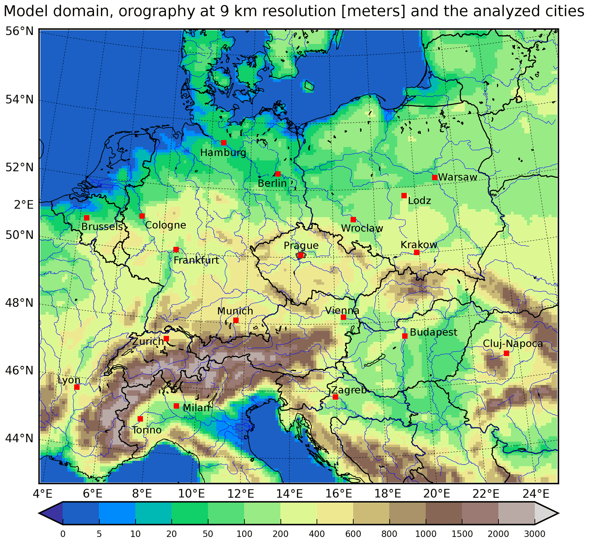
Figure 1The 9 km × 9 km resolution model domain and the resolved terrain in meters including the cities analyzed in the study (red squares).
2.3 Model simulations
The study intends to evaluate the urbanization impact on air quality, while we attempted to decompose the total impact into individual contributors listed in the Introduction. This requires performing a series of model experiments with individual effects added gradually one by one to a reference state to end up with the real situation corresponding to full urbanization. In Huszar et al. (2018a, b) we performed a similar decomposition for the urban-induced meteorological effects (i.e., the UCMF) and their impact on air quality. Here we adopt this approach, but it will not concern the UCMF solely as in the mentioned works but the entire impact of urbanization, while UCMF will be treated as one effect.
The simulations performed are summarized in Tables 1 and 2 for RCM and the underlying CTM simulations, respectively. A pair of simulations was performed with both RegCM and WRF with (“Urban”) and without (“Nourban”) considering urban land surface. In the latter case, land use was replaced by “crops” as the most common rural land use type in the region analyzed. While all RegCM simulations and CAMx simulations driven by RegCM were performed on nested domains (9, 3, and 1 km), the WRF simulations and CAMx ones driven by WRF were done only over the parent 9 km domain as WRF served as a complementary model to account for the uncertainty in the driving meteorology, especially with regard to UCMF; note that the urban canopy model is different in WRF than in RegCM.
Table 1The list of RCM simulations performed.
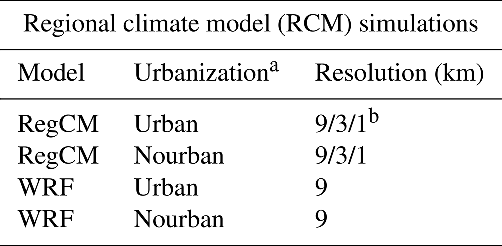
a Information on whether urban land surface was considered. “Nourban” means replacing the urban land surface by crops. b Simulation performed in a nested way at 9, 3, and 1 km horizontal grid resolution.
Table 2The list of CTM simulations performed with information on the effects considered. The “driving meteorology” and “driving meteorology (BVOC)” columns correspond to the information from Table 1 above, i.e., which RCM simulation from the “Urban”–“Nourban” pair was used.

∗ Information on whether the meteorology driving MEGAN accounted for the UCMF.
As for the CAMx simulations, they differ based on the inclusion of urbanized–rural land surface, the UCMF (acting on both atmospheric chemistry in general and on BVOC fluxes), and the urban emissions. In this regard, we performed six experiments summarized in Table 2. The reference experiment called ENNrrN represents the hypothetical background state without urban emissions and with the urban land surface replaced by rural land surface in RCMs and the CTM as well as in the BVOC model (MEGAN). The reference simulation is not to be confused with the preindustrial state: we assumed current climate (GHG – greenhouse gas – concentration) and current background large-scale chemical concentrations. In the next experiment, ENYrrN, only the urban emissions are considered (turned on). In the third experiment, ENYurN, the urban land use was turned on for the dry deposition in CAMx. In the fourth experiment, ENYuuN, the urban land use is also turned on for the biogenic emission model. In the fifth experiment, ENYuuU, both the urban land use and the UCMF are accounted for in the biogenic emissions model, and finally, in the sixth experiment, EUYuuU, all the urbanization-related effects are considered, representing the most realistic case.
In the first experiment wherein urban emissions are disregarded, we removed urban emissions only for the 19 cities chosen for the analysis. For the effect of rural–urban land use transformation on meteorological conditions, dry deposition, and biogenic emissions, we replaced the urban land by rural land over the entire domain (i.e., not only for the cities chosen). It is clear that this has an effect on the background level of air pollutants not only at local urban levels, but the effect is probably much smaller than local effects as (1) emissions from these areas were still considered, and (2) the urban meteorological effects from these (minor) urban areas have a rather small influence on air pollutants as the UCMF is also small (see, e.g., Huszar et al., 2014). In Fig. 1, we plot the model orography and the analyzed cities as red squares. For urban land use information used in our study, please refer to Karlický et al. (2020) (Figs. 1 and 2), who used identical land use as in our study.
Mathematically, with respect to the rural–urban transformation (RUT), the concentration ci of a pollutant i for a chosen city is given by
where ci,rural is the average concentration before RUT and Δci,RUT is the total impact of urbanization.
In this study, we are concerned about the contributors to Δci,RUT (regardless of their sign):
where Δci,EMIS, Δci,MET, Δci,LU_D, and Δci,BVOC are the impacts of urban emissions, the impact of the urban canopy meteorological forcing, the impact of modified land use on dry deposition, and the impact of modifications of BVOC emissions, denoted above as DEMIS, DMET, DLU_D, and DBVOC. The Δci,BVOC impact can further be decomposed into the part caused by modified land cover (reduced vegetation in terms of changes in leaf area index – LAI, DBVOC_L) and modified meteorological conditions (DBVOC_M):
These impacts will be calculated from the experiments listed in Table 2 in the following way (the experiment number is shown in parentheses).
It has to be noted that in reality these effects act simultaneously and feedbacks are present between them, so their effects are not additive. The way we calculated the individual impacts (contributors), however, allows us to consider them to be additive; i.e., their sum is the total impact of urbanization.
3.1 Validation
This model configuration (same input data, same domain) underwent a detailed validation including both meteorology and air quality in Huszar et al. (2020b, 2021). However, due to the fact that in our CAMx simulations, the newer version 7.10 was used instead of version 6.50, and instead of the CB5 we used the newer CB6 chemistry mechanism, we provide a brief account for validation. For comparison with observations, AirBase European air quality data (https://discomap.eea.europa.eu/map/fme/AirQualityExport.htm, last access: 27 September 2022) for the modeled years were used, while all urban- and suburban-type background stations (AirQualityStationArea indicates urban and/or suburban, and AirQualityStationType indicates background) were used from a subset of the analyzed cities. This sub-selection considered the largest cities from the total of 19 where sufficient numbers of stations were available.
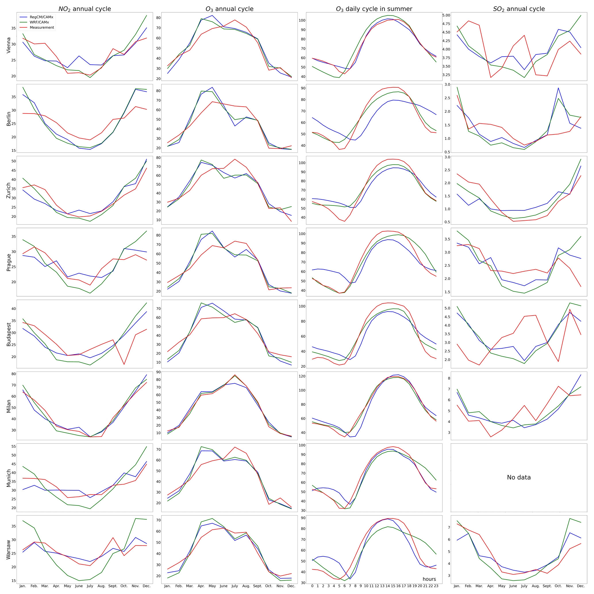
Figure 2Comparison of modeled (blue – RegCM/CAMx; green – WRF/CAMx) and measured (red; AirBase data) urban and suburban average monthly concentrations of NO2 (first column) and O3 (second column), the average JJA diurnal cycle of O3 (third column), and the average monthly concentrations of SO2 (fourth column) for 8 different cities selected from the total 19 considered in the study, namely Berlin, Budapest, Milan, Munich, Prague, Zurich, Vienna, and Warsaw (units: µg m−3). Data are averaged across all available urban- and suburban-type background stations within the chosen city. There are no data for SO2 in Munich as no corresponding measuring station was available.
In Fig. 2, the comparison of average monthly means of modeled and measured concentrations of the three analyzed pollutants is shown, while the full experiment (EUYuuU) was used, which represents the real case. For ozone, we also included the average summer diurnal cycle, as daily peak values are more important for this pollutant than the averages values. For Prague, results are taken from the 1 km nested domain; otherwise, they are extracted from the 9 km regional domain. For NO2, there is a generally acceptable match between the model and observations, with model biases up to 10 µg m−3. While concentrations from January to April are usually underestimated, during summer, CAMx generates a positive bias, except in Berlin, where there is an underestimation of NO2 from March to September and an overestimation during the rest of the year. During late autumn the model bias is usually negative, with large differences between cities. The WRF-driven CAMx concentrations are usually lower then for RegCM/CAMx during summer, which means higher model bias (up to −10 µg m−3). During winter, WRF/CAMx gives higher concentrations than RegCM/CAMx, resulting in a smaller bias.
For O3, both RegCM/CAMx and WRF/CAMx capture the annual cycle well, with some overestimation of concentrations during late spring (by about 10–20 µg m−3) and an underestimation during late summer (by a similar magnitude). In general, these two simulations are very similar. During winter, there is a small negative (up to −10 µg m−3) model bias present. The summer diurnal cycles show good agreement in the basic measured pattern, including the timing of the maximum. The maximum values are sometimes underestimated (by up to 20 µg m−3 for some cities), especially for the RegCM-driven runs. In general, WRF meteorology causes higher simulated maximum ozone. During nighttime, ozone is often overestimated by around 10–20 µg m−3, and clearly, the WRF-driven run performs better during this part of the day.
Regarding SO2, the model fails to capture the annual cycle well. During winter, both models usually underestimate the concentrations by up to 1–2 µg m−3 except in Budapest and Berlin, where overestimation occurs in the model. During summer, measured SO2 concentrations are usually smaller and the models somewhat reflect this fact, but large biases are still present and the models are unable to correctly capture the annual cycle for some cities (e.g., Budapest and Vienna).
3.2 The overall impact of individual contributors to RUT
Firstly, we evaluated the impact of individual contributors to the RUT as well as the total impact in terms of 2015–2016 DJF and JJA averages (in the case of ozone as a summer average only), averaged across the chosen cities and the model ensemble (i.e., average of the RegCM- and WRF-driven runs). Values are taken from the grid box covering the center of a particular city. The results are shown in Fig. 3 as box plots showing the first and third quartiles as well as the median values and the minimum and maximum. The analysis showed (as expected) that from the four contributors to RUT, two are much stronger than the other two. Therefore, in the plots, we separated them from the minors ones (including the total impact).
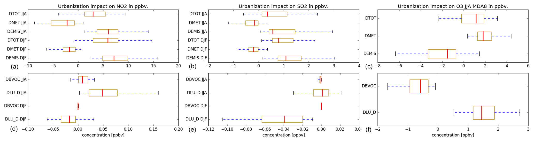
Figure 3The 2015–2016 DJF and JJA averaged impact of each contributor to the rural–urban transformation including the total impact averaged over all chosen cities for NO2, SO2, and O3 in parts per billion by volume (ppbv). In the case of ozone, only the summer averaged MDA8 (maximum daily 8 h average) is shown. The box plots show the 25 % to 75 % quantiles including the minimum and maximum value across all cities. The red line shows the median. Values are taken from the model grid cell that covers the city center. Panels (a)–(c) show the two main contributors including the total impact (DEMIS, DMET, and DTOT), while panels (d)–(f) show the minor contributors (DLU_D and DBVOC).
For all three gas-phase pollutants, the impact of emissions (DEMIS) is the largest in magnitude in both seasons. For NO2 it ranges (i.e., the 25th to 75th percentile) from 4 to about 8 ppbv and from 5 to 10 ppbv for JJA and DJF, respectively. For SO2, the numbers are somewhat smaller, as cities, at least in the region in focus, are not such strong SO2 emitters (compared to NO2): an increase by 0.4 to 1.5 and 0.8 to 1.6 ppbv for JJA and DJF, respectively, is seen. For O3, the impact on the summer maximum daily 8 h average concentration (MDA8) is characterized by a decrease due to titration (as expected) by 3 to 6 ppbv.
The impact of the urban canopy meteorological forcing (DMET) is characterized by a decrease for the primary pollutants: for NO2, the decrease is usually between 1 and 6 ppbv for JJA and between 1 and 3 ppbv in DJF with the maximum surpassing zero, meaning that in some cities, a slight increase was modeled. In the case of SO2, the impact of UCMF is smaller, with up to a 0.6 and 0.4 ppbv decrease in JJA and DJF, respectively. For O3, the impact is an increase of about 2 ppbv.
In the case of minor contributors, the impact of BVOCs is considerable for ozone only, and, as expected, for the other pollutants it acts as a minor modulator of the overall chemistry (e.g., influencing the hydroxyl budget), therefore having a very small impact. In the case of NO2, the impact is a slight increase by around 0.01 ppbv in JJA and negligible in winter. For SO2, it is near zero in both seasons. For ozone, which is directly influenced by biogenic emissions, the impact is a decrease by around 0.4 to 1 ppbv as a JJA average. The impact of modified dry deposition due to urbanized land use is characterized by an increase (0.02 to 0.08 ppbv) for NO2 in JJA and an opposite impact in winter (around 0.01 to 0.04 ppbv decrease). For SO2, the impact in summer can be both negative and positive (from −0.01 to 0.01 ppbv) with a near-zero average. In winter, there is a decrease by about 0.02 to 0.07 ppbv. For ozone, the impact of land use change is an increase between 1 and 2 ppbv.
Finally, the total impact is an increase for all pollutants and quantities: for NO2 it is about 1–5 ppbv in JJA and 4–8 ppbv in DJF, and for SO2 it ranges from 0 to 1 ppbv in JJA and about 0.5 to 1 ppbv in DJF. For JJA MDA8 ozone, the total impact is characterized by an increase up to 2 ppbv.
3.3 The spatial distribution of the impacts
The box plots presented above give an overview of the averaged impact across all the cities including the distribution around the median value. To obtain spatially resolved information, we also plotted the 2D distribution of the individual contributors here.
3.3.1 The impact of urban emissions (DEMIS)
In Fig. 4 the DJF and JJA average spatial impact of urban emissions (DEMIS) on the near-surface concentrations of NO2, SO2, and O3 is shown.
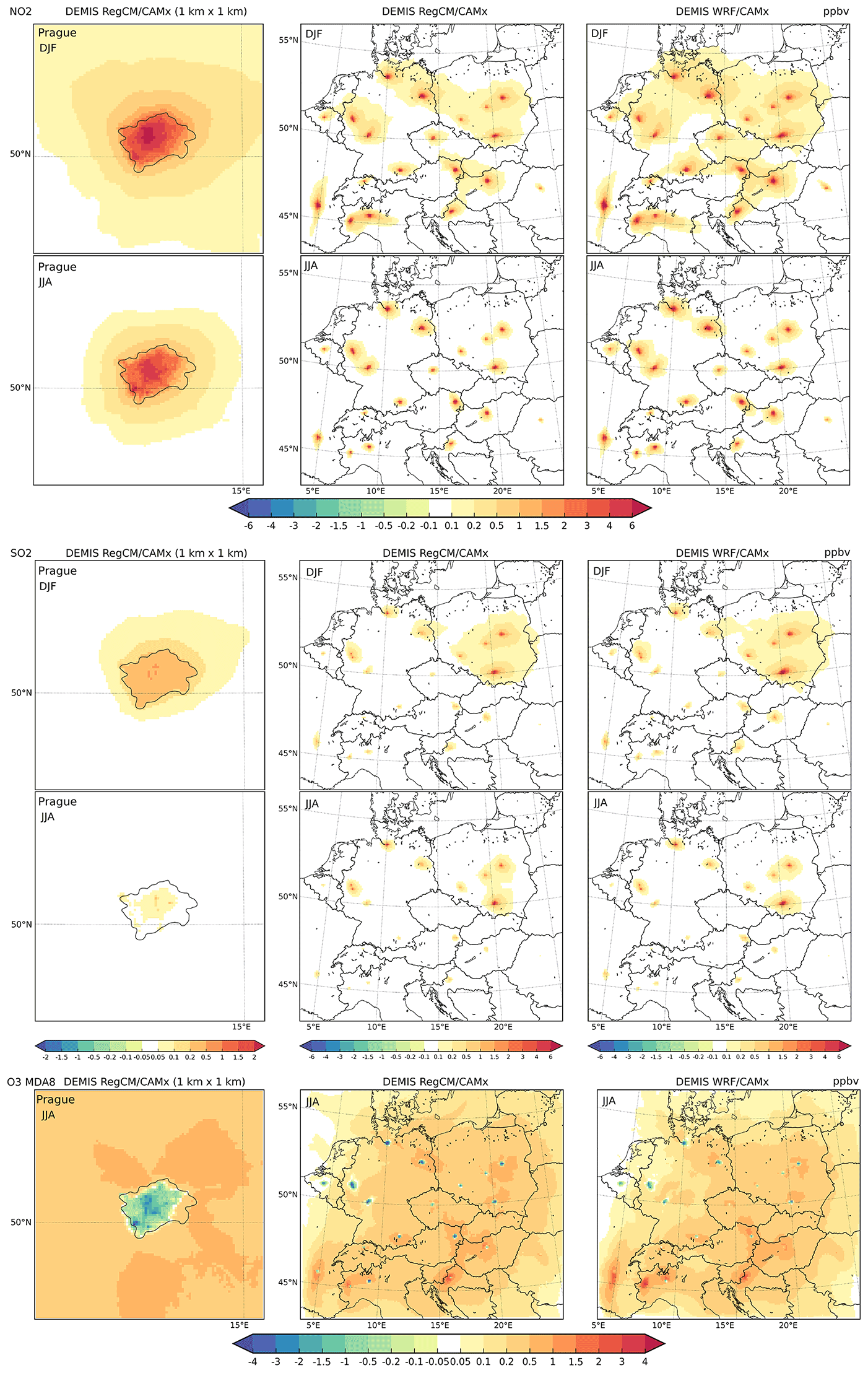
Figure 4The spatial distribution of the 2015–2016 average emission impact (DEMIS) for NO2 DJF and JJA (first and second row), SO2 DJF and JJA (third and fourth row), and JJA MDA8 O3 (fifth row). Columns represent the results from the 1 km RegCM/CAMx (detail of Prague), 9 km RegCM/CAMx, and 9 km WRF/CAMx simulations. Units are in parts per billion by volume (ppbv).
In the case of NO2, the impact reaches 4–6 ppbv in the core of the cities and remains high over surrounding areas (up to 0.5 ppbv over large areas in DJF, especially in the WRF-driven simulations). In summer, the spatial extent of the emission impact is smaller: below 0.1 ppbv over rural areas. The result from Prague at high resolution reveals that the high emission impact is concentrated in the very center of the city (reaching 4–6 ppbv).
For SO2, there is a larger spread between cities with large contributions over Poland reaching 6 ppbv (in both seasons), while for other cities, the contribution is smaller: up to 2–3 ppbv. The contribution over rural areas is large in Poland (up to 0.2 ppbv) but remains below 0.1 ppbv in other regions. The impact of emissions over Prague reaches 1 ppbv in DJF with contributions up to 0.1 ppbv in its vicinity. In summer, due to low emissions (SO2 is emitted largely by heating) the contributions are very small, reaching 0.5 ppbv in some hot spots within the city.
Ozone is usually titrated in city centers, which corresponds to the impact of emissions on its concentrations. They decreased over cities by up to 3–4 ppbv, while further from cities, where urban NOx mixes with rural emissions, an ozone increase occurs of up to 1 ppbv as MDA8. Over Prague, the decrease is limited to the city area. Over its vicinity, the impact becomes positive with a 0.5–1 ppbv increase (similarly as seen for other cities).
3.3.2 The impact of modified meteorological conditions (DMET)
Figure 5 presents the DJF and JJA average spatial impact of the urban canopy meteorological forcing (DMET) on the near-surface concentrations of NO2, SO2, and O3.
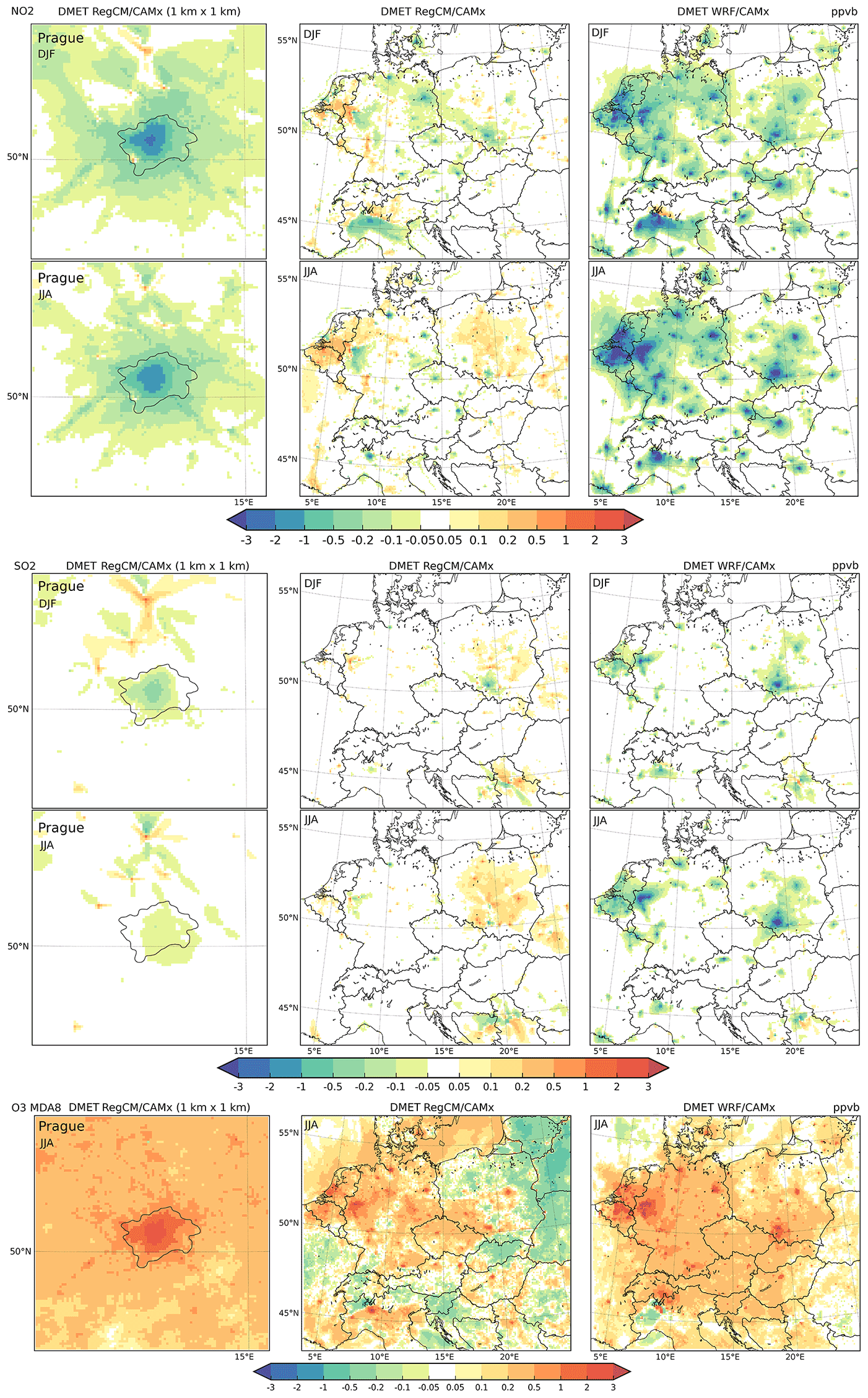
Figure 5The spatial distribution of the 2015–2016 average impact of the urban canopy meteorological forcing (UCMF) DMET on NO2 DJF and JJA (first and second row), SO2 DJF and JJA (third and fourth row), and JJA MDA8 O3 (fifth row). Columns represent the results from the 1 km RegCM/CAMx (detail of Prague), 9 km RegCM/CAMx, and 9 km WRF/CAMx simulations. Units are in parts per billion by volume (ppbv).
In the case of NO2, while for RegCM/CAMx the impact is usually characterized by a decrease by 1–2 ppbv with some urban areas even showing an increase (up to 2 ppbv), for WRF/CAMx a clear decrease occurs of up to 3 ppbv. For Prague, the highest decreases are modeled in the city center, reaching about 3 ppbv in summer and about 2 ppbv in winter. In general, the winter impact is comparable to summer (slightly stronger for WRF/CAMx).
For SO2 the impact is weaker and constitutes both decreases (in cities) and increases (over their vicinity) with changes in the range −3 to 3 ppbv. In the case of WRF/CAMx simulations, the impact is more straightforward with the decrease dominating, reaching 3 ppbv in both seasons.
Finally, summer MDA8 ozone increases due to UCMF by up to 2–3 ppbv over cities, while over rural areas, a slight decrease is modeled of up to 1 ppbv appearing in the RegCM/CAMx simulation. Over Prague, the largest increases are modeled in the city center, reaching 2–3 ppbv.
3.3.3 The impact of dry deposition modifications (DLUC_D)
The impact of urban land cover via modified dry deposition (DLU_D) is plotted in Fig. 6. In general, the impacts are much smaller for NO2 and SO2 than seen for the emission or the UCMF impact for these pollutants above. For NO2, the DJF and JJA impacts differ in sign (in accordance with the box plots seen in Fig. 3) and the spatial distribution is somewhat different in WRF/CAMx than in RegCM/CAMx. In DJF, NO2 concentrations decreased over cities by up to 0.04 ppbv, with some higher decreases over Italy (Milan) of up to 0.1 ppbv. In the WRF-driven experiment, some increases over the Benelux states are also seen, reaching 0.06 ppbv. For Prague, the decrease is maximal in the city center reaching 0.04 ppbv. During JJA, the DLU_D impact is positive, reaching 0.1 ppbv in both models with some slight decreases around Milan. Over Prague, the increase is even stronger and exceeds 0.05 ppbv.
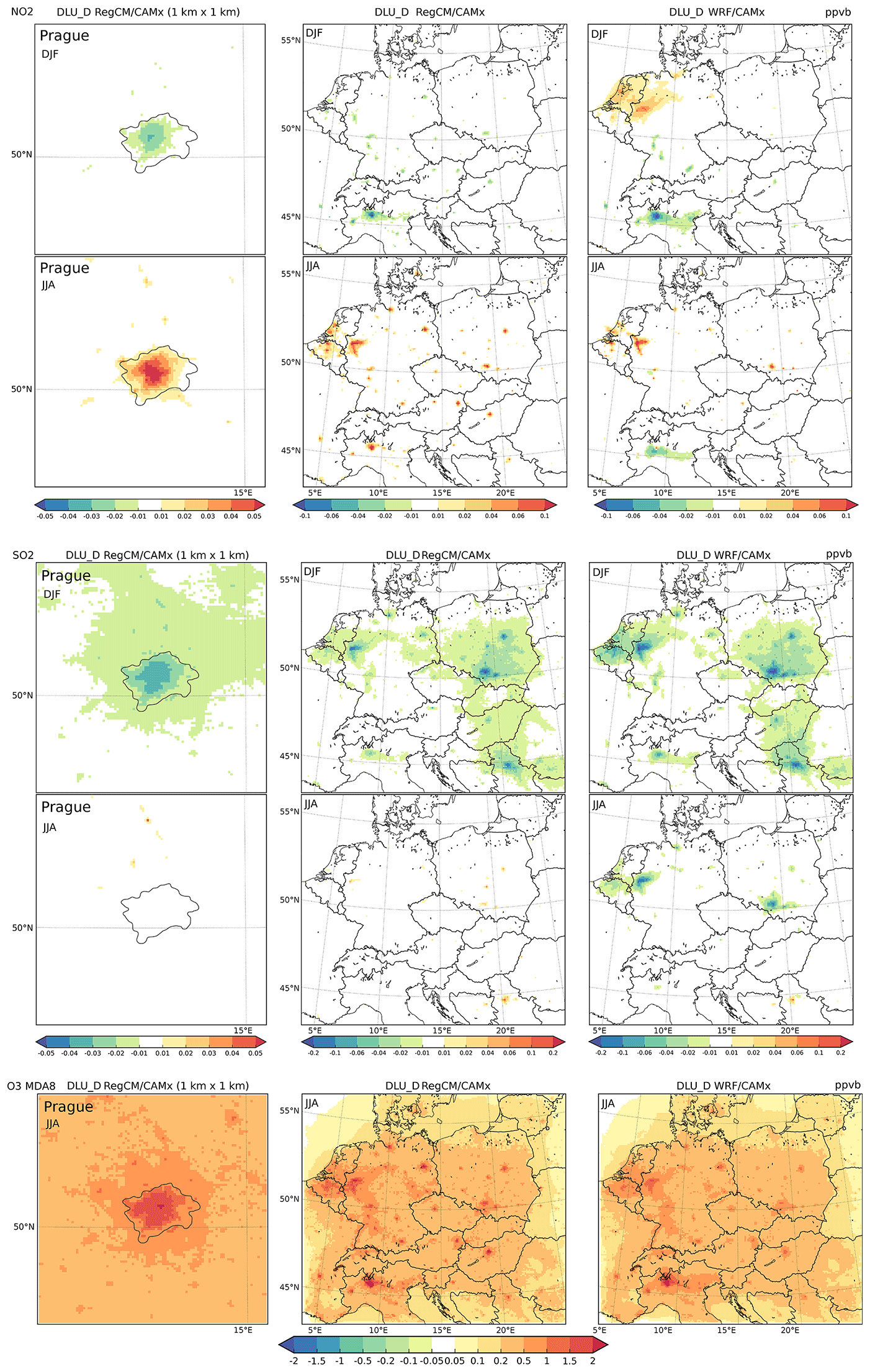
Figure 6The spatial distribution of the 2015–2016 average impact of the urban land cover via dry deposition modifications (DLU_D) on NO2 DJF and JJA (first and second row), SO2 DJF and JJA (third and fourth row), and JJA MDA8 O3 (fifth row). Columns represent the results from the 1 km RegCM/CAMx (detail of Prague), 9 km RegCM/CAMx, and 9 km WRF/CAMx simulations. Units are in parts per billion by volume (ppbv).
For SO2, there are clear decreases modeled during DJF, reaching 0.1–0.2 ppbv over city centers. The impacts are slightly stronger in WRF-driven CAMx runs and are about −0.03 ppbv over Prague's center. During JJA, the SO2 response is very small and positive in the RegCM/CAMx experiments with up to a 0.1 ppbv increase in some city centers, especially over eastern Europe where SO2 emissions are higher. Decreases similar to the DJF impact remained in the WRF/CAMx simulation. Over Prague, almost zero impact is modeled (between −0.01 and 0.01 ppbv with some positive impact around strong point sources north from the city).
A much stronger response to changes in dry deposition is modeled for summer O3, with a clear increase reaching 2 ppbv in city centers and being high over rural areas too (up to 1 ppbv increase). Over Prague, the increase is usually 1.5–2 ppbv, exceeding 2 ppbv in the very core of the city.

Figure 7The spatial distribution of the 2015–2016 average impact of the urban land cover on deposition velocities of NO2 (a, b), SO2 (c, d), and O3 (e, f) for DJF (a, c, e) and JJA (b, d, f) (mm s−1) for the RegCM-driven 9 km CAMx simulations.
To facilitate the interpretation of the simulated responses of concentrations to DLU_D, we also mapped the geographical distribution of the DLU_D impact on the deposition velocities (DV is standardly provided in CAMx output), as seen in Fig. 7 taken from the RegCM-driven CAMx simulations (and not showing the Prague 1 km case). For NO2, dry deposition velocities decreased by around 0.2 mm s−1 in DJF, and a stronger decrease, reaching −0.6 mm s−1, in city centers is modeled in JJA. For SO2, the DJF and JJA maps differ in sign. For winter, deposition velocities increased in cities by up to 0.4–0.6 mm s−1, while during summer, similar decreases are simulated compared to NO2 (around −0.4 to −0.6 mm s−1). For O3, both seasons are characterized by decreases: by around 0.2 mm s−1 in DJF with stronger decreases in city centers in JJA, reaching −1.5 mm s−1. The WRF/CAMx impacts are very similar and are not shown here.
3.3.4 The impact of biogenic emissions (DBVOC)
The urbanization-induced changes in BVOC emissions (via reduced vegetation cover and modified temperatures; DBVOC) and their consequent effect on summer ozone and NO2 concentrations are plotted in Fig. 8. As BVOC emissions are of minor importance in winter and the effect on SO2 is almost zero, we show only the summer impacts for these two pollutants. For NO2, the DBVOC impact results in increases usually up to 0.06 ppbv, while much stronger increases are modeled over northern Italy (around Milan) of around 0.1 ppbv in both RegCM- and WRF-driven simulations. For Prague, the maximum increase is 0.2–0.3 ppbv.
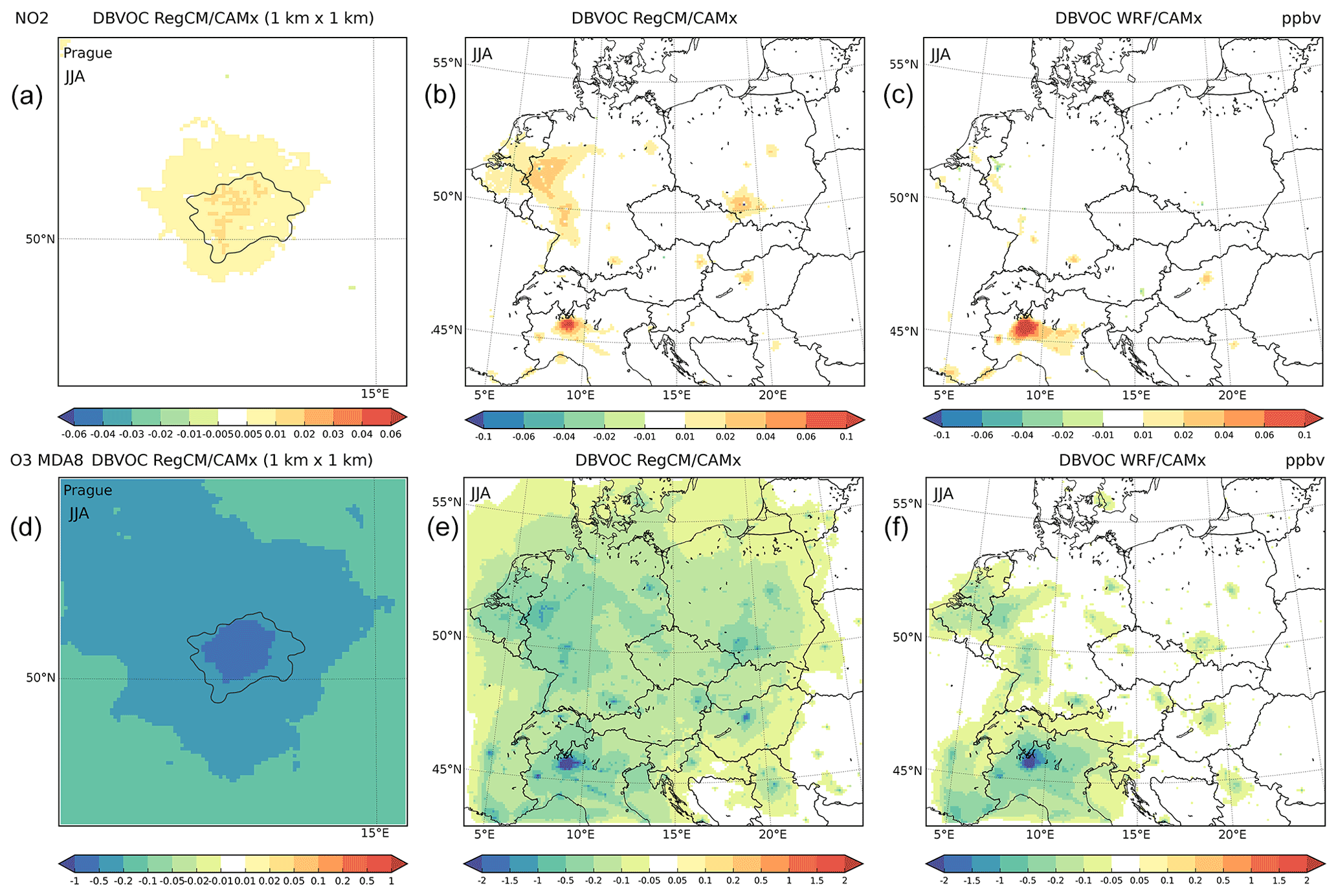
Figure 8The spatial distribution of the 2015–2016 average impact of urbanization due to modifications of biogenic emissions (DBVOC) on JJA average NO2 (a–c) and summer MDA8 O3 (d–f). Columns represent the results from the 1 km RegCM/CAMx (detail of Prague), 9 km RegCM/CAMx, and 9 km WRF/CAMx simulations. Units are in parts per billion by volume (ppbv).
For O3, decreases are modeled reaching −1 ppbv over many cities and reaching −0.2 to −0.5 ppbv over rural areas (in the RegCM-driven experiment). A stronger decrease is modeled (again) over northern Italy, with up to −2 ppbv over Milan. Prague is characterized by a decrease usually between −0.5 and −1 ppbv.

Figure 9The absolute (upper row; units mol km−2 h−1) and relative change (lower row; units in %) in 2015–2016 JJA averaged isoprene (ISOP) emissions decomposed into the part caused by reduced vegetation (via leaf area index; DBVOC_L) and the part caused by modified meteorology (DBVOC_M). The first and third columns show the change due to DBVOC_L taking the rural (NU) and urban (U) meteorological conditions as a reference, respectively. In the second and fourth columns, the changes due to urban meteorological effects (UCMF) are shown (DBVOC_M) taking the rural (NU) and urban (U) vegetation as a reference, respectively.
The impacts presented above are the result of modified BVOC emissions; therefore, we also plotted the summer changes in isoprene (ISOP) as a major component of such emissions. As changes in these emissions are the result of two components constituted of vegetation change via LAI change (DBVOC_L) and modification of meteorological conditions (the UCMF; denoted DBVOC_M in the Introduction), we plotted the two contributors separately in Fig. 9 as absolute and relative change. We were also interested in whether the reference with respect to which the change is calculated matters. In others words, what is the difference between the DBVOC_L calculated with rural (NOURBAN, see Table 1) meteorology and DBVOC_L calculated with urban meteorology (URBAN in Table 1)? Similarly for DBVOC_M, it is calculated with both rural LAI and that adapted for urban conditions. The impact of vegetation change is an expected decrease in isoprene emissions by up to 15 mol km−2 h−1, with higher values over the southern part of the domain, often representing a 80 %–90 % decrease in relative numbers, especially for larger and dense urban areas like Milan (Italy). For smaller urban areas the decrease is around −5 % to −20 % (many of the grid cells are only partly covered by urban areas, so the emission decrease is correspondingly small). As seen from the figure, the changes calculated at rural and urban meteorological conditions are very similar (the case with urban meteorology is slightly higher). Regarding the isoprene emission modifications due to UCMF, they are usually much smaller (usually less than 0.05 mol km−2 h−1 or less than 0.5 % in relative numbers). At some urban areas over Germany as well as over northern Italy and southern France, the change can reach 0.4 to 0.6 mol km−2 h−1, peaking at 1–2 mol km−2 h−1 over Italian urban areas, representing a 5 %–10 % relative increase. DBVOC_M is somewhat smaller if calculated with urban land cover, which is expected as the strongest meteorological modifications due to UCMF are over cities, but in this case they affect a non-vegetated surface, which implies smaller effects. In summary, the BVOC emission changes associated with vegetation change are much more important than the modifications due to UCMF.
3.4 The diurnal variation of the impacts
Urban emissions have a strong diurnal cycle caused by the typical cycle of human activities during the day. Moreover, the urban-land-surface-triggered meteorological modifications (UCMF) also have a strong diurnal pattern; e.g., temperature is impacted most during night, and the wind impacts and turbulence modifications are the strongest during noon. (Huszar et al., 2018a, 2020a). Thus, it is clear that the individual contributors to RUT analyzed here are expected to also have a diurnal cycle. Figure 10 presents these cycles for the four contributors and three analyzed pollutants.

Figure 10The 2015–2016 average diurnal cycle of the individual contributors to RUT for NO2 (a, d), SO2 (b, e), and O3 (c, f) as a DJF (a–c) and JJA (d–f) average. The brown and blue lines stand for the two stronger contributors (DEMIS and DMET, left y axis), while red and green stand for the weaker contributors (DLU_D and DBVOC, right y axis). Units are in parts per billion by volume (ppbv). Times are in UTC (i.e., the local time is +2 h in JJA and +1 h in DJF).
For NO2 the diurnal pattern for the emissions impact (DEMIS) follows the expected shape, with two peaks during morning and evening rush hours reaching 10–12 and 9–11 ppbv in DJF and JJA, respectively. The diurnal cycle for the UCMF impact (DMET) is negative throughout the whole day, with the peak decrease during evening hours reaching −5 and −8 ppbv in DJF and JJA, respectively. In the case of the impact of modified dry deposition (DLU_D), it has a somewhat different pattern in the two seasons. In DJF, it is negative throughout the day with a strong peak during morning hours (−0.04 ppbv) and a smaller evening peak (−0.03 ppbv). In summer, this impact is positive almost during the whole day with two peaks during morning and early evening hours reaching 0.18–0.2 ppbv, while during night, the impact can be slightly negative up to −0.04 ppbv. The impact of BVOC changes (DBVOC) is very small during winter with negative values peaking at less than −0.01 ppbv. During summer, the impact is stronger with a clear positive peak during evening hours reaching 0.06 ppbv.
In the case of SO2, the diurnal pattern for the impact of emissions and UCMF is similar to NO2. The emissions impact peaks at morning and evening rush hours for JJA, reaching 2.6–2.8 ppbv, while in DJF, the maximum impact is reached at evening hours and the impact remains high during the whole night (around 2.5–3 ppbv). The DMET impact is negative with an evening peak reaching −0.06 and −0.03 in DJF and JJA, respectively. The impact on dry deposition is negative in JJA with maximum impacts during morning and evening hours reaching −0.05 to −0.07 ppbv. During JJA, the impact is positive during the day with increases of up to 0.03 ppbv and decreases during night of up to −0.04 ppbv. We already saw in the box plots and also expected that the impact of BVOC emission change has an almost zero effect on SO2, which is not directly chemically tied to VOC chemistry.
Finally, for ozone, the impact of urban emissions is a decrease with two peaks during morning and evening hours reaching −10 to −12 ppbv in DJF and −8 to −10 ppbv in JJA. The impact of UCMF shows a clear increase peaking during evening hours, reaching around 5 and 10 ppbv during DJF and JJA, respectively. The impact of modifications of dry deposition is positive throughout the day with a strong peak during noon to early evening hours – during DJF, the peaks reach 0.2 ppbv, while a much stronger increase is modeled during summer reaching 1.5–2 ppbv. The impact of BVOC changes on ozone is virtually zero during DJF and negative during JJA, with a peak decrease around noon reaching 1 ppbv.
We also evaluated the diurnal cycle of the impact on deposition velocities, as this helps the interpretation of the DLU_D. In Fig. 11 the 2015–2016 winter and summer average of the DV diurnal cycle for the three analyzed pollutants is plotted as are the absolute values corresponding to the rural (“Nourban”) case. In the case of NO2, DVs are reduced when turning rural land use into urban land use, and the maximum decrease occurs during noon to early afternoon, reaching −0.4 mm s−1 in DJF with a stronger decrease reaching −3 mm s−1 in JJA, while during night, the change is close to zero. Similar decreases are calculated for ozone with somewhat smaller nocturnal values in DJF and a bit weaker decrease during summer peak values. For SO2, the impact on DV is different between DJF and JJA. During DJF, DV increases by 0.6 mm s−1 during night, while a smaller increase is calculated around noontime (0.2 mm s−1). During JJA, DV change for SO2 is slightly above zero and a strong negative peak occurs during the day, reaching about −1.5 to −2 mm s−1. Comparing with the absolute values, the impact of urban land use change in winter can reach −10 % to −20 % for ozone and NO2, while it is 20 %–30 % for sulfur dioxide. In summer the decrease is even higher, reaching 50 % for ozone and NO2, while for SO2, the relative decrease is about 30 %–40 %.
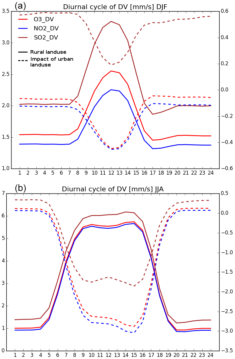
Figure 11The diurnal cycle of the rural deposition velocities (DV; solid lines; left y axis) and the impact of urbanization (dashed lines; right y axis) for 2015–2016 DJF (a) and JJA (b) for NO2 (blue), SO2 (brown), and O3 (red) (mm s−1).
We presented an analysis of the different contributors to the overall impact of urbanization (what we called here the rural–urban transformation; RUT) on urban gas-phase air pollutant concentrations. We focused on the four most important contributors to RUT, namely the impact of urban emissions (DEMIS), the impact of the urban canopy meteorological forcing on pollutant chemistry and transport (DMET), the impact of modified dry deposition due to the land cover modifications (DLU_D), and the impact of modified biogenic emissions due to modified land cover (and associated vegetation change) and modified meteorological conditions (DBVOC). By performing multiple simulations wherein each contributor of RUT was added one by one to the reference state representing land without urban land cover and urban emissions, we could quantify them individually.
The validation showed a reasonable range of model bias, and the annual cycles of pollutant concentrations for ozone and NO2 were well captured. The same is true for the model ability to resolve the diurnal cycle of ozone. Regarding NO2 biases, our results show a clear improvement from our previous study in Huszar et al. (2021), which used an almost identical setup and the same emissions input. It is clear that this improvement also cannot be explained by improved meteorology as the driving RegCM and CAMx simulations were the same. The only probable explanation is that the improvements were achieved by updating the chemistry mechanism in our simulations from CB5 to CB6r5. Indeed, CB6 was added to CAMx to take into account the long-lived organic compounds formed by peroxy radical reactions, which serve as an inhibitor of OH recycling and reduces NOx removal by OH oxidation (Cao et al., 2021). Previously, Luecken et al. (2019) also found a better model performance for reactive nitrogen when CB6 was used instead of CB-V. The slight deviation of the monthly cycles from observed values is probably caused by incorrect annual temporal disaggregation profiles, which are dependent only on the emission activity sector but not on the geographic location. Some studies using older chemistry mechanism also obtained larger NO2 biases (Karlický et al., 2017; Tucella et al., 2012), which suggests that the accuracy of the chemistry mechanism is probably very important. For ozone, monthly values were well represented by our model system, and the choice of the chemistry mechanism probably contributed to this, as in older studies using CB5 (or even the older CB-IV) (Zanis et al., 2011; Huszar et al., 2016a, 2020b) the biases were higher (moreover, the latter study used the same emission data as here) and were often caused by a strong nighttime bias, which seems to be partly removed in our study. Further, our results show similar model–observation agreement as the large online coupled model comparison study by Im et al. (2015). In the case of SO2, the model is rather unable to correctly resolve the annual cycle of near-surface concentrations. We also saw this behavior in a similar manner in Huszar et al. (2016a) and in Karlický et al. (2017), and it points to deficiencies in the annual profile used to time-disaggregate annual emissions to monthly ones. The SO2 biases can also be caused by wrong vertical turbulent mixing as large quantities of this pollutant are emitted from tall stacks and they have to mixed down to the surface layer, which is greatly influenced by the model representation of vertical eddy diffusivities. These are especially important in urban areas, and large uncertainty still persists in their calculation (Huszar et al., 2020a). In summary, for NO2 and O3 we did not identify substantial model biases in simulating urban near-surface concentrations of the analyzed pollutants. For sulfur dioxide, our model failed to correctly resolve the annual cycle, which suggests that the impact of urban SO2 emissions can also be overestimated or underestimated depending on the model bias and should be perceived with caution.
The total impact of urbanization on NO2 was calculated to around 3 (1 ÷ 5) ppbv in summer and 6 (3 ÷ 8) ppbv in winter. These numbers are smaller than the annual mean contributions calculated for 2001–2010 in Huszar et al. (2016a), and higher contributions were also modeled by Im and Kanakidou (2012); however, both simulated only the effect of urban emissions without considering the effect of the UCMF, which decreases near-surface concentrations (see further). The total impact on SO2 is between 0 and 1 ppbv in summer and 0.5–1.3 in winter, which is a smaller contribution than in Huszar et al. (2016a) due to much lower sulfur emissions in 2015 compared to the 2005 emissions used there and due to not considering the UCMF effects in the earlier study. The total average contribution for ozone summer MDA8 is about 1.5 (0 ÷ 2) ppbv. In Huszar et al. (2016a) for an ensemble of central European cities and Im et al. (2011a, b) for Mediterranean cities a decrease in ozone was shown (and increase over rural areas, similar to our results), but they accounted for only the urban emission impact. Indeed, urbanization via the UCMF increases ozone concentrations (Kim et al., 2015; Huszar et al., 2018a, 2020b), which can offset the decrease seen solely due to urban emissions. For all three pollutants, the effect of emissions (DEMIS) is stronger than the total effect of urbanization (DTOT) due to the strong modulating effect of the urban canopy meteorological forcing. As already calculated by many (e.g., Wang et al., 2007, 2009; Struzewska and Kaminski, 2012; Zhu et al., 2015; Huszar et al., 2020a), vertical eddy diffusion is the most important component of UCMF, which is strongly enhanced above urban areas. Consequently, it leads to reduced near-surface concentrations of primary pollutants (e.g., NO2, SO2) and an increase in ozone due to reducing the titration by NO (Escudero et al., 2014; Xie et al., 2016a, b).
As for the impact of UCMF (DMET) alone, our simulations showed a decrease by about 2 ppbv for NO2 and by 0.2–0.3 ppbv for SO2 (for both seasons) as well as an increase in summer MDA8 ozone by about 2 ppbv. These numbers fit previous findings in Sarrat et al. (2006), Struzewska and Kaminski (2012), Kim et al. (2015), and Huszar et al. (2018a, 2020b) well. They concluded that three main components play the most important role in UCMF: increased urban temperatures, decreased wind speeds, and increased vertical turbulent diffusion. While elevated surface temperatures favor photochemistry, they also result in stronger dry deposition as shown by Huszar et al. (2018a). Regarding the wind speed and turbulence effect, they are counteracting, which is seen in our results too, especially for SO2. For some of the cities, the impact is positive, meaning that the reduction of winds results in the emitted material remaining close to the sources. This was also previously seen by Huszar et al. (2018b) wherein the turbulence and wind effects were strongly competing. Our results also showed that the trade-off between wind and turbulence effects also depends on how the model simulates the UCMF components, and in our results, WRF produced a somewhat stronger increase in turbulence due to UCMF and weak wind reduction compared to RegCM. For ozone, the UCMF increased ozone by 2 ppbv, which is in line with previous finding in Huszar et al. (2018a), although they also included the effect of BVOC emissions modifications, which was treated separately here (see further). Due to urbanization, a similar increase was obtained by Martilli et al. (2003), Jiang et al. (2008), Xie et al. (2016a), and Jacobson et al. (2015). Some authors found somewhat larger increases for ozone (e.g., Ryu et al., 2013, for Seoul), but they adopted higher resolutions for the cities in focus and thus obtained higher peak impacts in urban centers (as seen in, e.g., Huszar et al., 2020b, too).
The diurnal cycle for the DMET impact shows a very characteristic pattern. In the case of primary pollutants (NO2 and SO2) the decrease is strongest during evening hours. This can be explained by the largest absolute values during evening hours, which is further closely related to the maximum impact of emissions – a similar finding was found by Huszar et al. (2018a) and also by Huszar et al. (2018b) for primary aerosol components. Indeed, the quantity of gases transported due to enhanced turbulence is proportional to the absolute concentrations, and these are highest during evening hours due to strong emissions during transport rush hours. For ozone, the diurnal pattern contains a maximum during evening hours corresponding to the largest impact on NO2. This justifies the argument that the UCMF-induced ozone increase is mainly caused by reduced NOx due to strong urban dilution and consequent reduced titration.
Besides the strong and well-documented air quality effects of urban emissions (DEMIS) and UCMF (DMET), our study also looked at two other contributors to RUT, which were expected to be smaller but which were not yet quantified in detail. Our study, at least according to the knowledge of the authors, is among the first to explicitly investigate the effect of urbanization from the perspective of change in dry deposition (DLU_D), and we also looked at the effect of urbanization-induced changes in BVOC emissions, which was examined only partly in previous studies (e.g., Huszar et al., 2018a; Li et al., 2019).
The impact due to modified dry deposition shows a distinct picture for NO2 between summer and winter. For both seasons, reduced deposition velocities were modeled with stronger decreases in summer (the WRF-driven CAMx results are not shown as they differ from the RegCM-driven only slightly). Reduced deposition velocities result in higher concentrations, which is opposite to what was modeled. To better understand what controls the NO2 budget, we have to consider the simultaneous effect of ozone changes due to changes in dry deposition. Our results showed strong increases in ozone concentrations, which is probably caused by suppressed dry deposition (for winter too; not shown in this paper). This is expected as many studies showed strong dependence of ozone concentrations on ozone deposition (Tao et al., 2013; Park et al., 2014) and ozone deposition on land use information (Mcdonald-Buller et al., 2001). When examining the concentration response to changed dry deposition, one has to consider the indirect impact due to other influenced pollutants, and pollutants responsible for NO2 removal (e.g., by reaction NO2+OH, forming nitric acid, or by NO2+O3, forming the nitrate radical) were probably impacted by weaker dry deposition (as seen for ozone), resulting in decreases in NO2, outweighing the direct impact of dry deposition change, as seen for winter. Another factor playing a role in decreases in NO2 can be the much larger (by 50 %) deposition velocities for nitric acid (HNO3) in the Zhang model for the urban land use type compared to crops or similar rural land use (i.e., “Nourban” case). Large dry deposition for HNO3 in turn results in a decrease in this compound, which reduces the recycling of NO2 from it (by photolysis). On the other hand, in summer, such effects can amplify the impact. In this season the deposition-induced ozone changes probably played a role in the NO2 budget. It has to realized that a major pathway of NO2 chemistry in cities is oxidation of NO with ozone (). Increased ozone concentrations thus result in more NO oxidizing to NO2.
In the case of sulfur dioxide, deposition increased in winter, which resulted in a clear decrease in near-surface concentration. The dry deposition of sulfur strongly differs between wet and dry soils (Hardacre et al., 2021), and according to Zhang et al. (2003), who provided the dry deposition scheme we adopted, the deposition velocities (DVs) are higher for urban areas than for crops or similar rural land use types (which was considered in the “Nourban” case). In winter, soils are very often wet, which could result in an increase in DVs (especially during night as seen in our results) and a consequent decrease in concentrations. During summer, DVs decreased for SO2; however, there is no clear increase in concentrations, i.e., almost no change in RegCM-driven simulations and even some decrease in the WRF-driven ones. This again can be explained by the impact of deposition on other chemical species which cause removal of SO2, typically oxidation by the OH radical.
The impact of BVOC emission changes (DBVOC) is straightforward and expected for ozone, i.e., a decrease by 0.5–1 ppbv. BVOC emissions decreased due to urbanization-related reduction of vegetation (i.e., reduction of vegetation fraction and leaf area index) and increased due to higher urban temperatures (within the action of the UCMF). This latter effect was smaller, resulting in the dominance of the first effect and an overall decrease in emissions, which is a similar result as in, e.g., Li et al. (2019). As ozone chemistry in cities in Europe (and also North American and Asian megacities) is characterized by a VOC-controlled regime with a high ratio (Beekmann and Vautard, 2010; Xue et al., 2014), ozone quickly responds to changes in VOC emissions; i.e., it decreases with decreasing BVOC emissions. This is in accordance with previous studies: e.g., Song et al. (2008) reported an 10 % decrease in ozone concentrations. The reduction in ozone was shown to be largest during daytime, which is in accordance with the largest BVOC emissions. Previously, Huszar et al. (2018a) reported ozone increases due to BVOC changes due to UCMF alone (i.e., not considering the impact of reduced vegetation) of the order of up to 0.1 ppbv. Our study showed that if vegetation modifications related to urbanization are added, this increase is outweighed by a much stronger decrease due to lower BVOC emissions.
Simultaneously with the DBVOC-related ozone decrease, we calculated a small summer increase in NO2 by about 0.01 ppbv. This cannot be explained by potentially reduced NO concentrations and suppressed NO2 formation with the reaction of ozone (titration), as NO also increased slightly as the result of DBVOC (not shown explicitly in this study). Moreover, soil NOx emissions in MEGAN also decreased slightly due to urban land use transformation. Reduced BVOC emissions result in reduced peroxy radical (RO2) concentrations, which is an important oxidation pathway to form NO2 from NO (Geng et al., 2011) and would result in a decrease in NO2. There must therefore be another compensating mechanism responsible for NOx increase, and this is probably the reduced concentrations of NOx sinks. One of the important urban contributors to this are PANs (peroxy acetyl nitrates), and as biogenic VOCs are a major contributor to urban PAN concentrations, it can be expected that with decreased BVOC emissions, the PAN sink is reduced, resulting in higher NOx concentrations (Fischer et al., 2014; Toma et al., 2019). Another reason can lie in reaction with the OH radical, which is reduced if ozone is reduced. In short, the relatively small positive NO2 response to urbanization-induced biogenic emissions changes is probably a simultaneous action of multiple indirect chemical pathways, and deeper process-based analysis should be performed to explicitly show the contribution and trade-off of each of them. The strongest changes modeled for Milan, Italy, can be explained by its relatively warm climate and large size, making the BVOC emission reduction strong and thus having a stronger effect on ozone and NO2 (via secondary effects discussed above).
The diurnal patterns of different RUT contributors are explainable by the typical diurnal patterns of anthropogenic emissions and also by the UCMF's diurnal cycle. For the impact of urban emissions only, the DEMIS impact clearly resembles the emissions which peak in cities at morning and evening rush hours (Huszar et al., 2021). The impact of urbanization-induced meteorological changes (UCMF) is governed by increased vertical eddy diffusion, which is strongest during daytime (Huszar et al., 2020a) and causes a decrease in primary pollutant concentrations as well as an increase in ozone (reduced titration; Huszar et al., 2018a). As the impact is proportional to the absolute concentrations, it is again largest during morning and (especially) early evening rush hours, during which even stronger vertical mixing usually occurs. A somewhat more complex explanation is needed regarding the diurnal pattern of the land use change and dry deposition impact. For ozone, a strong decrease occurs during daytime, which is related to high daytime absolute values and a stronger decrease in deposition velocities during the day due to urbanized land surface. Over vegetated surface, ozone dry deposition is determined mainly by stomatal resistance, which is lowest during daytime, meaning that the ozone dry deposition velocities are highest during the day (Park et al., 2014). When the surface is urbanized, the vegetation's role in dry deposition becomes very small and this daytime peak of DV disappears, which results in the strongest decrease in DV during the day. The diurnal cycle of the DLU_D for NO2 is probably the combined effect of decreased DVs, which are strongest during the day and logically lead to increased concentrations, and the reduction due to a dry-deposition-induced increase in ozone concentrations (see above regarding how this might influence the NO2 concentrations). As this latter occurs during noontime, the resulting shape of the diurnal pattern of DLU_D for nitrogen dioxide has a double peak. Finally, the diurnal cycle of the response of SO2 to dry deposition changes due to urban land surface has a clear daytime peak during winter when the impact is smallest. This is in line with the smallest increase in DV for SO2, which occurs during daytime. During summer, the shape of the diurnal cycle for the impact on SO2 is similar; however, the values are higher, making the peaks reach positive values. These can be attributed to the summer decrease in DV, peaking during daytime, which leads to an increase in concentrations. A more interesting feature is that the impact goes to negative values during nighttime for this pollutant. This cannot be explained by the DVs alone, and, as already said above, some secondary chemical effects play a role; e.g., increased ozone concentration leads to increased OH radical, which can lead to increased oxidation of SO2, as already suggested earlier. The diurnal impact of DBVOC for ozone in summer has a clear daytime negative peak, which is connected to the highest BVOC emissions occurring at this time of the day. As the most important factor in the urbanization impact on BVOC is the reduction of vegetation, the highest reduction of emissions is expected to occur during daytime, and in a VOC-limited environment this results in a stronger suppression of ozone production (i.e., leading to reduction). In the case of NO2, the DBVOC impact is probably connected to decreased PAN, which is an important sink for NOx (as already said above). As the absolute NOx concentrations peak during evening rush hours, this sink has the strongest effect during this time, creating the evening peak of DBVOC for NO2.
Our results further showed that the magnitude of each contributor for Prague is higher at the 1 km resolution nested domain than at 9 km resolution. This was already seen in previous studies focusing on the impact of UCMF in extreme air pollution (Huszar et al., 2020b) and also concerned the magnitude of the UCMF itself (e.g., the temperature increases due to urbanization have a higher city core peak at higher resolution). This was further seen regarding the impact of urban emissions only in Huszar et al. (2021). It can be assumed that if a nested domain approach at high resolution was applied to other cities, the impacts would have a stronger city core peak than at 9 km resolution.
To summarize our finding, we showed with an ensemble of 19 central European cities that the strongest contributors to the impact of rural-to-urban transformation are the urban emissions themselves (increase concentrations for nitrogen dioxide and sulfur dioxide and decrease those for ozone) and the urban canopy meteorological forcing (decreases the concentration of primary pollutants and increases those of ozone). They have to be accounted for simultaneously as the impact of urban emissions without considering UCMF can lead to overestimation of the impact (Huszar et al., 2021). Additionally, we quantified two weaker contributors. The effect of modified land use on dry deposition and the effect of modified biogenic emissions have 1 order weaker magnitude than emissions and the UCMF. However, we showed that for summer ozone, these are strong and of comparable order as the two strongest impacts. In other words, when analyzing the overall impact of urbanization on air pollution for ozone, all four contributors have to be accounted for, having a similar order of magnitude, while for primary gas-phase pollutants (i.e., NO2 and SO2), the two weaker contributors are by at least 1 order of magnitude smaller and the error made is small if they are neglected.
Finally, we must stress that we focused on cities from a relatively small region, meaning the cities do not constitute substantially different climates and the typical “rural” vegetation was considered to be crops. In other parts of the world, e.g., tropical areas, rural-to-urban transformation takes place over different vegetation cover and, e.g., the impact of modified BVOC emissions could be much stronger than in the case of central European cities. Further, it has to be noted that some secondary effects of modified pollutant concentrations can potentially also play a role via the direct and indirect radiative effect of emissions. The direct effect of aerosols can alter photolysis rates and temperatures, influencing air chemistry (Han et al., 2020; Wang et al., 2022). It was further shown by many that aerosol emitted by urban areas modulates the vertical structure of the atmosphere, resulting in modification of stability and/or convection (Miao et al., 2020; Slater et al., 2022; Fan et al., 2020; Yu et al., 2020), which in turn can modify the vertical mixing or precipitation (Zhou et al., 2020; López-Romero et al., 2021); this finally feeds back to influence species concentration via wet deposition and mixing. Our study was an offline coupled one, meaning that no feedbacks from species concentrations via radiation and cloud–rain microphysics were accounted for. These studies, however, indicate that to obtain an even more comprehensive picture of the total RUT impact, these secondary effects also have to be taken into account in the future.
The RegCM4.7 model is freely available for public use at https://github.com/ICTP/RegCM (last access: 17 August 2022; Giuliani, 2021). CAMx version 7.10 is available at http://camx-wp.azurewebsites.net/download/source (last access: 27 September 2022; CAMx, 2022; Ramboll, 2020). The RegCM2CAMx meteorological preprocessor used to convert RegCM outputs to CAMx inputs and the MEGAN v2.10 code as used by the authors are available upon request from the main author. The complete model configuration and all the simulated data (three-dimensional hourly data) used for the analysis are stored at the Department of Atmospheric Physics, Charles University data storage facilities (about 5 TB), and are available upon request from the main author. The observational data from the AirBase database can be obtained from https://discomap.eea.europa.eu/map/fme/AirQualityExport.htm (EEA, 2021). The REZZO and ATEM emission data are not publicly available; however, the providers (the Czech Hydrometeorological Institute and ATEM – Atelier of Ecological Models) can provide the data upon request.
PH created the concept and designed the experiments. PH and JK performed the model simulations. LB, ML, and KS contributed to input data preparation, model configuration, and analysis of the outputs. APPP contributed to the validation. All authors contributed to the paper.
The contact author has declared that none of the authors has any competing interests.
Publisher's note: Copernicus Publications remains neutral with regard to jurisdictional claims in published maps and institutional affiliations.
We acknowledge the CAMS-REG-APv1.1 emissions dataset provided by the Copernicus Atmosphere Monitoring Service, the Air Pollution Sources Register (REZZO) dataset provided by the Czech Hydrometeorological Institute, and the ATEM Traffic Emissions dataset provided by ATEM (Studio of Ecological Models). We also acknowledge the providers of AirBase European Air Quality data (https://www.eea.europa.eu/data-and-maps/data/aqereporting-9, last access: 28 September 2022).
This research has been supported by the Grantová Agentura České Republiky (grant no. 19-10747Y) and the Univerzita Karlova v Praze (grant nos. 260581/2021 and Q47).
This paper was edited by Kostas Tsigaridis and reviewed by two anonymous referees.
Beekmann, M. and Vautard, R.: A modelling study of photochemical regimes over Europe: robustness and variability, Atmos. Chem. Phys., 10, 10067–10084, https://doi.org/10.5194/acp-10-10067-2010, 2010. a
Benešová, N., Belda, M., Eben, K., Geletič, J., Huszár, P., Juruš, P., Krč, P., Resler, J., and Vlček, O.: New open source emission processor for air quality models, in: Proceedings of Abstracts 11th International Conference on Air Quality Science and Application, Barcelona, Spain, 12–16 March 2018, University of Hertfordshire, https://doi.org/10.18745/PB.19829, 2018. a
Bougeault, P. and Lacarrère, P.: Parameterization of orography-induced turbulence in a meso-beta-scale model, Mon. Weather Rev., 117, 1872–1890, 1989. a
Buchholz, R. R., Emmons, L. K., Tilmes, S., and The CESM2 Development Team: CESM2.1/CAM-chem Instantaneous Output for Boundary Conditions, UCAR/NCAR – Atmospheric Chemistry Observations and Modeling Laboratory. Subset used Lat: 10 to 80, Lon: −20 to 50, December 2014–January 2017 [data set], https://doi.org/10.5065/NMP7-EP60, 2019. a
Burkholder, J. B., Sander, S. P., Abbatt, J. P. D., Barker, J. R., Huie, R. E., Kolb, C. E., Kurylo, M. J., Orkin, V. L., Wilmouth, D. M., and Wine, P. H.: Chemical kinetics and photochemical data for use in atmospheric studies: evaluation number 18, JPL Publication 15-10, Jet Propulsion Laboratory, Pasadena, CA, http://jpldataeval.jpl.nasa.gov (last access: 27 September 2022), 2019. a
Butler, T. M. and Lawrence, M. G.: The influence of megacities on global atmospheric chemistry: a modelling study, Environ. Chem., 6, 219–225, https://doi.org/10.1071/EN08110, 2009. a
Byun, D. W. and Ching, J. K. S.: Science Algorithms of the EPA Model-3 Community Multiscale Air Quality (CMAQ) Modeling System, Office of Research and Development, U.S. EPA, North Carolina, EPA/600/R-99/030, 1999. a
CAMx: Comprehensive Air Quality Model With Extensions version 7.10 code, Ramboll US Corporation, Novato, CA 94945, USA [code], http://camx-wp.azurewebsites.net/download/source (last access: 27 September 2022), 2020. a
Cao, L., Li, S., and Sun, L.: Study of different Carbon Bond 6 (CB6) mechanisms by using a concentration sensitivity analysis, Atmos. Chem. Phys., 21, 12687–12714, https://doi.org/10.5194/acp-21-12687-2021, 2021. a
Chen, S. and Sun, W.: A one-dimensional time dependent cloud model, J. Meteorol. Soc. Jpn., 80, 99-118, 2002. a
Cherin, N., Roustan, Y., Musson-Genon, L., and Seigneur, C.: Modelling atmospheric dry deposition in urban areas using an urban canopy approach, Geosci. Model Dev., 8, 893–910, https://doi.org/10.5194/gmd-8-893-2015, 2015. a
Ďoubalová, J., Huszár, P., Eben, K., Benešová, N., Belda, M., Vlček, O., Karlický, J., Geletič, J., and Halenka, T.: High Resolution Air Quality Forecasting Over Prague within the URBI PRAGENSI Project: Model Performance During the Winter Period and the Effect of Urban Parameterization on PM, Atmosphere, 11, 625, https://doi.org/10.3390/atmos11060625, 2020. a
Emmons, L. K., Schwantes, R. H., Orlando, J. J., Tyndall, G., Kinnison, D., Lamarque, J.-F., Marsh, D., Mills, M. J., Tilmes, S., Bardeen, C., Buchholtz, R. R., Conley, A., Gettelman, A., Garcia, R., Simpson, I., Blake, D. R., Meinardi, S., and Petron, G.: The Chemistry Mechanism in the Community Earth System Model version 2 (CESM2), J. Adv. Model. Earth Sys., 12, e2019MS001882, https://doi.org/10.1029/2019MS001882, 2020. a
Escudero, M., Lozano, A., Hierro, J., del Valle, J., and Mantilla, E.: Urban influence on increasing ozone concentrations in a characteristic Mediterranean agglomeration, Atmos. Environ., 99, 322–332, https://doi.org/10.1016/j.atmosenv.2014.09.061, 2014. a
European Environment Agency (EEA): Air quality in Europe – 2019 report, EEA Report No 10/2019, https://doi.org/10.2800/822355, 2019. a, b
EEA: Air Quality e-Reporting products on EEA data service: E1a and E2a data sets, European Environment Agency, Copenhagen, Denmark [data set], https://discomap.eea.europa.eu/map/fme/AirQualityExport.htm (last access: 27 September 2022), 2021. a
Fan, J., Zhang, Y., Li, Z., Hu, J., and Rosenfeld, D.: Urbanization-induced land and aerosol impacts on sea-breeze circulation and convective precipitation, Atmos. Chem. Phys., 20, 14163–14182, https://doi.org/10.5194/acp-20-14163-2020, 2020. a
Finardi, S., Silibello, C., D'Allura, A., and Radice, P.: Analysis of pollutants exchange between the Po Valley and the surrounding European region, Urban Climate, 10, 682–702, https://doi.org/10.1016/j.uclim.2014.02.002, 2014. a
Fischer, E. V., Jacob, D. J., Yantosca, R. M., Sulprizio, M. P., Millet, D. B., Mao, J., Paulot, F., Singh, H. B., Roiger, A., Ries, L., Talbot, R. W., Dzepina, K., and Pandey Deolal, S.: Atmospheric peroxyacetyl nitrate (PAN): a global budget and source attribution, Atmos. Chem. Phys., 14, 2679–2698, https://doi.org/10.5194/acp-14-2679-2014, 2014. a
Folberth, G. A., Butler, T. M., Collins, W. J., and Rumbold, S. T.: Megacities and climate change – A brief overview, Environ. Pollut., 203, 235–242, https://doi.org/10.1016/j.envpol.2014.09.004, 2015. a
Galmarini, S., Makar, P., Clifton, O. E., Hogrefe, C., Bash, J. O., Bellasio, R., Bianconi, R., Bieser, J., Butler, T., Ducker, J., Flemming, J., Hodzic, A., Holmes, C. D., Kioutsioukis, I., Kranenburg, R., Lupascu, A., Perez-Camanyo, J. L., Pleim, J., Ryu, Y.-H., San Jose, R., Schwede, D., Silva, S., and Wolke, R.: Technical note: AQMEII4 Activity 1: evaluation of wet and dry deposition schemes as an integral part of regional-scale air quality models, Atmos. Chem. Phys., 21, 15663–15697, https://doi.org/10.5194/acp-21-15663-2021, 2021. a
Ganbat, G., Baik, J. J., and Ryu, Y. H.: A numerical study of the interactions of urban breeze circulation with mountain slope winds, Theor. App. Clim., 120, 123–135, 2015. a
Gao, J. and O'Neill, B. C.: Mapping global urban land for the 21st century with data-driven simulations and Shared Socioeconomic Pathways, Nat. Commun., 11, 2302, https://doi.org/10.1038/s41467-020-15788-7, 2020. a
Geng, F., Tie, X., Guenther, A., Li, G., Cao, J., and Harley, P.: Effect of isoprene emissions from major forests on ozone formation in the city of Shanghai, China, Atmos. Chem. Phys., 11, 10449–10459, https://doi.org/10.5194/acp-11-10449-2011, 2011. a
Giorgi, F., Coppola, E., Solmon, F., Mariotti, L., Sylla, M., Bi, X., Elguindi, N., Diro, G. T., Nair, V., Giuliani, G., Cozzini, S., Guettler, I., O'Brien, T. A., Tawfi, A. B., Shalaby, A., Zakey, A., Steiner, A., Stordal, F., Sloan, L., and Brankovic, C.: RegCM4: model description and preliminary tests over multiple CORDEX domains, Clim. Res., 52, 7–29, 2012. a
Giuliani, G.: The Regional Climate Model version 4.7 source code, ICTP, GitHub [code], https://github.com/ICTP/RegCM (last access: 17 August 2022), 2021. a
Granier, C. S., Darras, H., Denier van der Gon, J., Doubalova, N., Elguindi, B., Galle, M., Gauss, M., Guevara, J.-P., Jalkanen, J., and Kuenen, C.: The Copernicus Atmosphere Monitoring Service Global and Regional Emissions, Report April 2019 version [Research Report], ECMWF, Reading, UK, https://doi.org/10.24380/d0bn-kx16, 2019. a
Grell, G.: Prognostic evaluation of assumptions used by cumulus parameterizations, Mon. Weather Rev., 121, 764–787, 1993. a
Guenther, A., Karl, T., Harley, P., Wiedinmyer, C., Palmer, P. I., and Geron, C.: Estimates of global terrestrial isoprene emissions using MEGAN (Model of Emissions of Gases and Aerosols from Nature), Atmos. Chem. Phys., 6, 3181–3210, https://doi.org/10.5194/acp-6-3181-2006, 2006. a
Guenther, A. B., Jiang, X., Heald, C. L., Sakulyanontvittaya, T., Duhl, T., Emmons, L. K., and Wang, X.: The Model of Emissions of Gases and Aerosols from Nature version 2.1 (MEGAN2.1): an extended and updated framework for modeling biogenic emissions, Geosci. Model Dev., 5, 1471–1492, https://doi.org/10.5194/gmd-5-1471-2012, 2012. a
Guo, Y., Yan, C., Liu, Y., Qiao, X., Zheng, F., Zhang, Y., Zhou, Y., Li, C., Fan, X., Lin, Z., Feng, Z., Zhang, Y., Zheng, P., Tian, L., Nie, W., Wang, Z., Huang, D., Daellenbach, K. R., Yao, L., Dada, L., Bianchi, F., Jiang, J., Liu, Y., Kerminen, V.-M., and Kulmala, M.: Seasonal variation in oxygenated organic molecules in urban Beijing and their contribution to secondary organic aerosol, Atmos. Chem. Phys., 22, 10077–10097, https://doi.org/10.5194/acp-22-10077-2022, 2022. a
Guttikunda, K. S., Carmichael, G. R., Calori, G., Eck, C., and Woo, J.-H.: The contribution of megacities to regional sulfur pollution in Asia, Atmos. Environ., 37, 11–22, https://doi.org/10.1016/S1352-2310(02)00821-X, 2003. a, b
Guttikunda, S. K., Tang, Y., Carmichael, G. R., Kurata, G., Pan, L., Streets, D. G., Woo, J.-H., Thongboonchoo, N., and Fried, A.: Impacts of Asian megacity emissions on regional air quality during spring 2001, J. Geophys. Res., 110, D20301, https://doi.org/10.1029/2004JD004921, 2005. a
Han, W., Li, Z., Wu, F., Zhang, Y., Guo, J., Su, T., Cribb, M., Fan, J., Chen, T., Wei, J., and Lee, S.-S.: The mechanisms and seasonal differences of the impact of aerosols on daytime surface urban heat island effect, Atmos. Chem. Phys., 20, 6479–6493, https://doi.org/10.5194/acp-20-6479-2020, 2020. a
Hardacre, C., Mulcahy, J. P., Pope, R. J., Jones, C. G., Rumbold, S. T., Li, C., Johnson, C., and Turnock, S. T.: Evaluation of SO2, SO and an updated SO2 dry deposition parameterization in the United Kingdom Earth System Model, Atmos. Chem. Phys., 21, 18465–18497, https://doi.org/10.5194/acp-21-18465-2021, 2021. a, b
Hodnebrog, Õ., Stordal, F., and Berntsen, T. K.: Does the resolution of megacity emissions impact large scale ozone?, Atmos. Environ., 45, 6852–6862, 2011. a, b
Holtslag, A. A. M., de Bruijn, E. I. F., and Pan, H.-L.: A high resolution air mass transformation model for shortrange weather forecasting, Mon. Weather Rev., 118, 1561–1575, 1990. a
Hong, S.-Y., Dudhia, J., and Chen, S.-H.: A Revised Approach to Ice Microphysical Processes for the Bulk Parameterization of Clouds and Precipitation, Month. Weather Rev., 132, 103–120, https://doi.org/10.1175/1520-0493(2004)132<0103:ARATIM>2.0.CO;2, 2004. a
Hood, C., MacKenzie, I., Stocker, J., Johnson, K., Carruthers, D., Vieno, M., and Doherty, R.: Air quality simulations for London using a coupled regional-to-local modelling system, Atmos. Chem. Phys., 18, 11221–11245, https://doi.org/10.5194/acp-18-11221-2018, 2018. a
Huszar, P., Miksovsky, J., Pisoft, P., Belda, M., and Halenka, T.: Interactive coupling of a regional climate model and a chemistry transport model: evaluation and preliminary results on ozone and aerosol feedback, Clim. Res., 51, 59–88, https://doi.org/10.3354/cr01054, 2012. a
Huszar, P., Halenka, T., Belda, M., Zak, M., Sindelarova, K., and Miksovsky, J.: Regional climate model assessment of the urban land-surface forcing over central Europe, Atmos. Chem. Phys., 14, 12393–12413, https://doi.org/10.5194/acp-14-12393-2014, 2014. a, b, c, d, e
Huszar, P., Belda, M., and Halenka, T.: On the long-term impact of emissions from central European cities on regional air quality, Atmos. Chem. Phys., 16, 1331–1352, https://doi.org/10.5194/acp-16-1331-2016, 2016a. a, b, c, d, e, f, g, h, i, j, k
Huszár, P., Belda, M., Karlický, J., Pišoft, P., and Halenka, T.: The regional impact of urban emissions on climate over central Europe: present and future emission perspectives, Atmos. Chem. Phys., 16, 12993–13013, https://doi.org/10.5194/acp-16-12993-2016, 2016b. a
Huszar, P., Karlický, J., Belda, M., Halenka, T., and Pisoft, P.: The impact of urban canopy meteorological forcing on summer photochemistry, Atmos. Environ., 176, 209–228, https://doi.org/10.1016/j.atmosenv.2017.12.037, 2018a. a, b, c, d, e, f, g, h, i, j, k, l
Huszar, P., Belda, M., Karlický, J., Bardachova, T., Halenka, T., and Pisoft, P.: Impact of urban canopy meteorological forcing on aerosol concentrations, Atmos. Chem. Phys., 18, 14059–14078, https://doi.org/10.5194/acp-18-14059-2018, 2018b. a, b, c, d, e
Huszar, P., Karlický, J., Ďoubalová, J., Šindelářová, K., Nováková, T., Belda, M., Halenka, T., Žák, M., and Pišoft, P.: Urban canopy meteorological forcing and its impact on ozone and PM2.5: role of vertical turbulent transport, Atmos. Chem. Phys., 20, 1977–2016, https://doi.org/10.5194/acp-20-1977-2020, 2020a. a, b, c, d, e, f
Huszar, P., Karlický, J., Ďoubalová, J., Nováková, T., Šindelářová, K., Švábik, F., Belda, M., Halenka, T., and Žák, M.: The impact of urban land-surface on extreme air pollution over central Europe, Atmos. Chem. Phys., 20, 11655–11681, https://doi.org/10.5194/acp-20-11655-2020, 2020b. a, b, c, d, e, f, g
Huszar, P., Karlický, J., Marková, J., Nováková, T., Liaskoni, M., and Bartík, L.: The regional impact of urban emissions on air quality in Europe: the role of the urban canopy effects, Atmos. Chem. Phys., 21, 14309–14332, https://doi.org/10.5194/acp-21-14309-2021, 2021. a, b, c, d, e, f, g, h, i, j
Im, U. and Kanakidou, M.: Impacts of East Mediterranean megacity emissions on air quality, Atmos. Chem. Phys., 12, 6335–6355, https://doi.org/10.5194/acp-12-6335-2012, 2012. a, b, c, d, e
Im, U., Poupkou, A., Incecik, S., Markakis, K., Kindap, T., Unal, A., Melas, D., Yenigun, O., Topcu, O., Odman, M. T., Tayanc, M., and Guler, M.: The impact of anthropogenic and biogenic emissions on surface ozone concentrations in Istanbul, Sci. Total Environ., 409, 1255–1265, https://doi.org/10.1016/j.scitotenv.2010.12.026, 2011a. a, b
Im, U., Markakis, K., Poupkou, A., Melas, D., Unal, A., Gerasopoulos, E., Daskalakis, N., Kindap, T., and Kanakidou, M.: The impact of temperature changes on summer time ozone and its precursors in the Eastern Mediterranean, Atmos. Chem. Phys., 11, 3847–3864, https://doi.org/10.5194/acp-11-3847-2011, 2011b. a, b
Im, U., Bianconi, R., Solazzo, E., Kioutsioukis, I., Badia, A., Balzarini, A., Baró, R., Bellasio, R., Brunner, D., Chemel, C., Curci, G., Flemming, J., Forkel, R., Giordano, L., Jiménez-Guerrero, P., Hirtl, M., Hodzic, A., Honzak, L., Jorba, O., Knote, C., Kuenen, J. J., Makar, P. A., Manders-Groot, A., Neal, L., Pérez, J. L., Pirovano, G., Pouliot, G., San Jose, R., Savage, N., Schroder, W., Sokhi, R. S., Syrakov, D., Torian, A., Tuccella, P., Werhahn, J., Wolke, R., Yahya, K., Zabkar, R., Zhang, Y., Zhang, J., Hogrefe, C., and Galmarini, S.: Evaluation of operational on-line-coupled regional air quality models over Europe and North America in the context of AQMEII phase 2. Part I: Ozone, Atmos. Environ., 115, 404–420, https://doi.org/10.1016/j.atmosenv.2014.09.042, 2015. a
IUPAC: Task Group on Atmospheric Chemical Kinetic Data Evaluation, http://iupac.pole-ether.fr/# (last access: 27 September 2022), 2019. a
Jacobson, M. Z., Nghiem, S. V., Sorichetta, A., and Whitney, N.: Ring of impact from the mega-urbanization of Beijing between 2000 and 2009, J. Geophys. Res., 120, 5740–5756, https://doi.org/10.1002/2014JD023008, 2015. a, b
Janssen, R. H. H., Tsimpidi, A. P., Karydis, V. A., Pozzer, A., Lelieveld, J., Crippa, M., Prévôt, A. S. H., Ait-Helal, W., Borbon, A., Sauvage, S., and Locoge, N.: Influence of local production and vertical transport on the organic aerosol budget over Paris, J. Geophys. Res., 122, 8276–8296, https://doi.org/10.1002/2016JD026402, 2017. a
Jiang, X., Wiedinmyer, C., Chen, F., Yang, Z.-L., and Lo, J. C.- F.: Predicted impacts of climate and land use change on surface ozone in the Houston, Texas, area, J. Geophys. Res., 113, D20312, https://doi.org/10.1029/2008JD009820, 2008. a
Kang, H., Zhu, B., de Leeuw, G., Yu, B., van der A, R. J., and Lu, W.: Impact of urban heat island on inorganic aerosol in the lower free troposphere: a case study in Hangzhou, China, Atmos. Chem. Phys., 22, 10623–10634, https://doi.org/10.5194/acp-22-10623-2022, 2022. a
Karlický, J., Huszár, P., and Halenka, T.: Validation of gas phase chemistry in the WRF-Chem model over Europe, Adv. Sci. Res., 14, 181–186, https://doi.org/10.5194/asr-14-181-2017, 2017. a, b
Karlický, J., Huszár, P., Halenka, T., Belda, M., Žák, M., Pišoft, P., and Mikšovský, J.: Multi-model comparison of urban heat island modelling approaches, Atmos. Chem. Phys., 18, 10655–10674, https://doi.org/10.5194/acp-18-10655-2018, 2018. a
Karlický, J., Huszár, P., Nováková, T., Belda, M., Švábik, F., Ďoubalová, J., and Halenka, T.: The “urban meteorology island”: a multi-model ensemble analysis, Atmos. Chem. Phys., 20, 15061–15077, https://doi.org/10.5194/acp-20-15061-2020, 2020. a, b, c
Kesselmeier, J. and Staudt, M.: Biogenic Volatile Organic Compounds (VOC): an overview on emission, physiology and ecology, J. Atmos. Chem., 33, 23–88, 1999. a
Khomenko, S., Cirach, M., Pereira-Barboza, E., Mueller, N., Barrera-Gómez, J., Rojas-Rueda, D., de Hoogh, K., Hoek, G., and Nieuwenhuijsen, M.: Premature mortality due to air pollution in European cities: a health impact assessment, Lancet Planetary Health, 5, 121–134, https://doi.org/10.1016/S2542-5196(20)30272-2, 2021. a
Kim, G., Lee, J., Lee, M.-I., and Kim, D.: Impacts of urbanization on atmospheric circulation and aerosol transport in a coastal environment simulated by the WRF-Chem coupled with urban canopy model, Atmos. Environ., 249, 118253, https://doi.org/10.1016/j.atmosenv.2021.118253, 2021. a
Kim, Y, Sartelet, K., Raut, J.-C., and Chazette, P.: Influence of an urban canopy model and PBL schemes on vertical mixing for air quality modeling over Greater Paris, Atmos. Environ., 107, 289–306, https://doi.org/10.1016/j.atmosenv.2015.02.011, 2015 a, b, c
Kusaka, H., Kondo, K., Kikegawa, Y., and Kimura, F.: A simple single-layer urban canopy model for atmospheric models: Comparison with multi-layer and slab models, Bound.-Lay. Meteorol., 101, 329–358, 2001. a
Lawrence, M. G., Butler, T. M., Steinkamp, J., Gurjar, B. R., and Lelieveld, J.: Regional pollution potentials of megacities and other major population centers, Atmos. Chem. Phys., 7, 3969–3987, https://doi.org/10.5194/acp-7-3969-2007, 2007. a, b
Lazaridis, M., Latos, M., Aleksandropoulou, V., How, Ø., Papayannis, A., and Tørseth, K.: Contribution of forest fire emissions to atmospheric pollution in Greece, Air. Qual. Atmos. Health., 1, 143–158, https://doi.org/10.1007/s11869-008-0020-0, 2008. a
Li, Y., Zhang, J., Sailor, D. J., and Ban-Weiss, G. A.: Effects of urbanization on regional meteorology and air quality in Southern California, Atmos. Chem. Phys., 19, 4439–4457, https://doi.org/10.5194/acp-19-4439-2019, 2019. a, b, c, d, e
Liao, J., Wang, T., Wang, X., Xie, M., Jiang, Z., Huang, X., and Zhu, J.: Impacts of different urban canopy schemes in WRF/Chem on regional climate and air quality in Yangtze River Delta, China, Atmos. Res., 145–146, 226–243, https://doi.org/10.1016/j.atmosres.2014.04.005, 2014. a
López-Romero, J. M., Montávez, J. P., Jerez, S., Lorente-Plazas, R., Palacios-Peña, L., and Jiménez-Guerrero, P.: Precipitation response to aerosol–radiation and aerosol–cloud interactions in regional climate simulations over Europe, Atmos. Chem. Phys., 21, 415–430, https://doi.org/10.5194/acp-21-415-2021, 2021. a
Louis, J. F.: A Parametric Model of Vertical Eddy Fluxes in the Atmosphere, Bound.-Lay. Meteorol., 17, 187-‐202, 1979. a
Luecken, D., Yarwood, G., and Hutzell, W.: Multipollutant modeling of ozone, reactive nitrogen and HAPs across the continental US with CMAQ-CB6, Atmos. Environ., 201, 62–72, https://doi.org/10.1016/j.atmosenv.2018.11.060, 2019. a
Markakis, K., Valari, M., Perrussel, O., Sanchez, O., and Honore, C.: Climate-forced air-quality modeling at the urban scale: sensitivity to model resolution, emissions and meteorology, Atmos. Chem. Phys., 15, 7703–7723, https://doi.org/10.5194/acp-15-7703-2015, 2015. a, b
Martilli, A., Roulet, Y.-A., Junier, M., Kirchner, F., Rotach, M. W., and Clappier, A.: On the impact of urban surface exchange parameterisations on air quality simulations: the Athens case, Atmos. Environ., 37, 4217–4231, https://doi.org/10.1016/S1352-2310(03)00564-8, 2003. a
Mcdonald-Buller, E., Wiedinmyer, C., Kimura, Y., and Allen, D.: Effects of land use data on dry deposition in a regional photochemical model for eastern Texas, J. Air Waste Manage. Assoc., 51, 1211–1218, https://doi.org/10.1080/10473289.2001.10464340, 2001. a, b
Mertens, M., Kerkweg, A., Grewe, V., Jöckel, P., and Sausen, R.: Attributing ozone and its precursors to land transport emissions in Europe and Germany, Atmos. Chem. Phys., 20, 7843–7873, https://doi.org/10.5194/acp-20-7843-2020, 2020. a
Miao, Y., Che, H., Zhang, X., and Liu, S.: Integrated impacts of synoptic forcing and aerosol radiative effect on boundary layer and pollution in the Beijing–Tianjin–Hebei region, China, Atmos. Chem. Phys., 20, 5899–5909, https://doi.org/10.5194/acp-20-5899-2020, 2020. a
Nenes, A., Pandis, S. N., and Pilinis, C.: ISORROPIA: a new thermodynamic equilibrium model for multiphase multicomponent inorganic aerosols, Aquat. Geochem., 4, 123–152, 1998. a
Nowak, D. J. and Dwyer, J. F.: Understanding the Benefits and Costs of Urban Forest Ecosystems, In: Urban and Community Forestry in the Northeast, edited by: Kuser, J. E., Springer Netherlands, 25–46, 2007. a
Oke, T., Mills, G., Christen, A., and Voogt, J.: Urban Climates, Cambridge University Press, https://doi.org/10.1017/9781139016476, 2017. a, b, c
Oke, T. R.: The energetic basis of the urban heat island, Q. J. Roy. Meteor. Soc., 108, 1–24, https://doi.org/10.1002/qj.49710845502, 1982. a
Oleson, K., Lawrence, D. M., Bonan, G. B., Drewniak, B., Huang, M., Koven, C. D., Levis, S., Li, F., Riley, W. J., Subin, Z. M., Swenson, S. C., Thornton, P. E., Bozbiyik, A., Fisher, R., Heald, C. L., Kluzek, E., Lamarque, J.-F., Lawrence, P. J., Leung, L. R., Lipscomb, W., Muszala, S., Ricciuto, D. M., Sacks, W., Sun, Y., Tang, J., and Yang, Z.-L.: Technical Description of version 4.5 of the Community Land Model (CLM), NCAR Technical Note NCAR/TN-503+STR, Boulder, Colorado, 420 pp., https://doi.org/10.5065/D6RR1W7M, 2013. a
Oleson, K. W., Bonan, G. B., Feddema, J., Vertenstein, M., and Grimmond, C. S. B.: An urban parameterization for a global climate model. 1. Formulation and evaluation for two cities, J. Appl. Meteor. Clim., 47, 1038–1060, 2008. a
Oleson, K. W., Bonan, G. B., Feddema, J., Vertenstein, M., and Kluzek, E.: Technical Description of an Urban Parameterization for the Community Land Model (CLMU), NCAR TECHNICAL NOTE NCAR/TN-480+STR, National Center for Atmospheric Research, Boulder, Co, USA, 61–88, https://doi.org/10.5065/D6K35RM9, 2010. a
Panagi, M., Fleming, Z. L., Monks, P. S., Ashfold, M. J., Wild, O., Hollaway, M., Zhang, Q., Squires, F. A., and Vande Hey, J. D.: Investigating the regional contributions to air pollution in Beijing: a dispersion modelling study using CO as a tracer, Atmos. Chem. Phys., 20, 2825–2838, https://doi.org/10.5194/acp-20-2825-2020, 2020. a
Panopoulou, A., Liakakou, E., Sauvage, S., Gros, V., Locoge, N., Stavroulas, I., Bonsang, B., Gerasopoulos, E., and Mihalopoulos, N.: Yearlong measurements of monoterpenes and isoprene in a Mediterranean city (Athens): Natural vs anthropogenic origin, Atmos. Environ., 243, 117803, https://doi.org/10.1016/j.atmosenv.2020.117803, 2020. a
Park, R. J., Hong, S. K., Kwon, H.-A., Kim, S., Guenther, A., Woo, J.-H., and Loughner, C. P.: An evaluation of ozone dry deposition simulations in East Asia, Atmos. Chem. Phys., 14, 7929–7940, https://doi.org/10.5194/acp-14-7929-2014, 2014. a, b
Passant, N.: Speciation of UK Emissions of Non-methane Volatile Organic Compounds, DEFRA, Oxon, UK, https://uk-air.defra.gov.uk/assets/documents/reports/empire/AEAT_ENV_0545_final_v2.pdf (last access: 27 September 2022), 2002. a
Ramboll: User's Guide Comprehensive Air Quality Model With Extensions Version 7.10, User Guide, Ramboll US Corporation, Novato, CA 94945, USA, https://camx-wp.azurewebsites.net/Files/CAMxUsersGuide_v7.10.pdf (last access: 27 September 2022), 2020. a, b
Ren, Y., Zhang, H., Wei, W., Wu, B., Cai, X., and Song, Y.: Effects of turbulence structure and urbanization on the heavy haze pollution process, Atmos. Chem. Phys., 19, 1041–1057, https://doi.org/10.5194/acp-19-1041-2019, 2019. a
Ribeiro, F. N. D., Oliveira, A. P., Soares, J., Miranda, R. M., Barlage, M., and Chen, F.: Effect of sea breeze propagation on the urban boundary layer of the metropolitan region of Sao Paulo, Brazil, Atmos. Res., 214, 174–188, https://doi.org/10.1016/j.atmosres.2018.07.015, 2018. a
Ryu, Y.-H., Baik, J.-J., Kwak, K.-H., Kim, S., and Moon, N.: Impacts of urban land-surface forcing on ozone air quality in the Seoul metropolitan area, Atmos. Chem. Phys., 13, 2177–2194, https://doi.org/10.5194/acp-13-2177-2013, 2013. a
Sarrat, C., Lemonsu, A., Masson, V., and Guedalia, D.: Impact of urban heat island on regional atmospheric pollution, Atmos. Environ., 40, 1743–1758, 2006. a
Seinfeld, J. H. and Pandis, S. N.: Atmospheric Chemistry and Physics: From Air Pollution to Climate Change, J. Wiley, New York, ISBN 978-1-118-94740-1, 1998. a
Simmons, A. J., Willett, K. M., Jones, P. D., Thorne, P. W., and Dee, D. P.: Low-frequency variations in surface atmospheric humidity, temperature and precipitation: inferences from reanalyses and monthly gridded observational datasets, J. Geophys. Res., 115, D01110, https://doi.org/10.1029/2009JD012442, 2010. a
Sindelarova, K., Granier, C., Bouarar, I., Guenther, A., Tilmes, S., Stavrakou, T., Müller, J.-F., Kuhn, U., Stefani, P., and Knorr, W.: Global data set of biogenic VOC emissions calculated by the MEGAN model over the last 30 years, Atmos. Chem. Phys., 14, 9317–9341, https://doi.org/10.5194/acp-14-9317-2014, 2014. a
Sindelarova, K., Markova, J., Simpson, D., Huszar, P., Karlicky, J., Darras, S., and Granier, C.: High-resolution biogenic global emission inventory for the time period 2000–2019 for air quality modelling, Earth Syst. Sci. Data, 14, 251–270, https://doi.org/10.5194/essd-14-251-2022, 2022. a
Situ, S., Guenther, A., Wang, X., Jiang, X., Turnipseed, A., Wu, Z., Bai, J., and Wang, X.: Impacts of seasonal and regional variability in biogenic VOC emissions on surface ozone in the Pearl River delta region, China, Atmos. Chem. Phys., 13, 11803–11817, https://doi.org/10.5194/acp-13-11803-2013, 2013. a
Skamarock, W. C., Klemp, J. B., Dudhia, J., Gill, D. O., Liu, Z., Berner, J., Wang, W., Powers, J. G., Duda, M. G., Barker, D. M., and Huang, X.-Y.: A Description of the Advanced Research WRF Version 4, NCAR Tech. Note NCAR/TN-556+STR, 145 pp. https://doi.org/10.5065/1dfh-6p97, 2019. a
Skyllakou, K., Murphy, B. N., Megaritis, A. G., Fountoukis, C., and Pandis, S. N.: Contributions of local and regional sources to fine PM in the megacity of Paris, Atmos. Chem. Phys., 14, 2343–2352, https://doi.org/10.5194/acp-14-2343-2014, 2014. a
Slater, J., Coe, H., McFiggans, G., Tonttila, J., and Romakkaniemi, S.: The effect of BC on aerosol–boundary layer feedback: potential implications for urban pollution episodes, Atmos. Chem. Phys., 22, 2937–2953, https://doi.org/10.5194/acp-22-2937-2022, 2022. a
Sokhi, R. S., Moussiopoulos, N., Baklanov, A., Bartzis, J., Coll, I., Finardi, S., Friedrich, R., Geels, C., Grönholm, T., Halenka, T., Ketzel, M., Maragkidou, A., Matthias, V., Moldanova, J., Ntziachristos, L., Schäfer, K., Suppan, P., Tsegas, G., Carmichael, G., Franco, V., Hanna, S., Jalkanen, J.-P., Velders, G. J. M., and Kukkonen, J.: Advances in air quality research – current and emerging challenges, Atmos. Chem. Phys., 22, 4615–4703, https://doi.org/10.5194/acp-22-4615-2022, 2022. a, b
Song, J., Webb, A., Parmenter, B. Allen, D. T., and McDonald-Buller, E.: The Impacts of Urbanization on Emissions and Air Quality: Comparison of Four Visions of Austin, Texas, Environ. Sci. Tech., 42, 7294–7300, https://doi.org/10.1021/es800645j, 2008. a, b, c, d
Stock, Z. S., Russo, M. R., Butler, T. M., Archibald, A. T., Lawrence, M. G., Telford, P. J., Abraham, N. L., and Pyle, J. A.: Modelling the impact of megacities on local, regional and global tropospheric ozone and the deposition of nitrogen species, Atmos. Chem. Phys., 13, 12215–12231, https://doi.org/10.5194/acp-13-12215-2013, 2013. a, b
Strader, R., Lurmann, F., and Pandis, S. N.: Evaluation of secondary organic aerosol formation in winter, Atmos. Environ., 33., 4849–4863, 1999. a
Struzewska, J. and Kaminski, J. W.: Impact of urban parameterization on high resolution air quality forecast with the GEM – AQ model, Atmos. Chem. Phys., 12, 10387–10404, https://doi.org/10.5194/acp-12-10387-2012, 2012. a, b, c
Tagaris, E., Sotiropoulou, R. E. P., Gounaris, N., Andronopoulos, S., and Vlachogiannis, D.: Impact of biogenic emissions on ozone and fine particles over Europe: Comparing effects of temperature increase and a potential anthropogenic NOx emissions abatement strategy, Atmos. Environ., 98, 214–223, https://doi.org/10.1016/j.atmosenv.2014.08.056, 2014. a
Tao, W., Liu, J., Ban-Weiss, G. A., Hauglustaine, D. A., Zhang, L., Zhang, Q., Cheng, Y., Yu, Y., and Tao, S.: Effects of urban land expansion on the regional meteorology and air quality of eastern China, Atmos. Chem. Phys., 15, 8597–8614, https://doi.org/10.5194/acp-15-8597-2015, 2015. a
Tao, Z., Santanello, J. A., Chin, M., Zhou, S., Tan, Q., Kemp, E. M., and Peters-Lidard, C. D.: Effect of land cover on atmospheric processes and air quality over the continental United States – a NASA Unified WRF (NU-WRF) model study, Atmos. Chem. Phys., 13, 6207–6226, https://doi.org/10.5194/acp-13-6207-2013, 2013. a
Thunis, P., Clappier, A., de Meij, A., Pisoni, E., Bessagnet, B., and Tarrason, L.: Why is the city's responsibility for its air pollution often underestimated? A focus on PM2.5, Atmos. Chem. Phys., 21, 18195–18212, https://doi.org/10.5194/acp-21-18195-2021, 2021. a
Tie, X., Brasseur, G., and Ying, Z.: Impact of model resolution on chemical ozone formation in Mexico City: application of the WRF-Chem model, Atmos. Chem. Phys., 10, 8983–8995, https://doi.org/10.5194/acp-10-8983-2010, 2010. a
Tie, X., Geng, F., Guenther, A., Cao, J., Greenberg, J., Zhang, R., Apel, E., Li, G., Weinheimer, A., Chen, J., and Cai, C.: Megacity impacts on regional ozone formation: observations and WRF-Chem modeling for the MIRAGE-Shanghai field campaign, Atmos. Chem. Phys., 13, 5655–5669, https://doi.org/10.5194/acp-13-5655-2013, 2013. a
Tiedtke, M.: A Comprehensive Mass Flux Scheme for Cumulus Parameterization in Large-Scale Models, Mon. Weather Rev., 117, 1779–1800, https://doi.org/10.1175/1520-0493(1989)117<1779:ACMFSF>2.0.CO;2, 1989. a
Timothy, M. and Lawrence, M. G.: The influence of megacities on global atmospheric chemistry: a modeling study, Environ. Chem., 6, 219–225, https://doi.org/10.1071/EN08110, 2009. a
Toma, S., Bertman, S., Groff, C., Xiong, F., Shepson, P. B., Romer, P., Duffey, K., Wooldridge, P., Cohen, R., Baumann, K., Edgerton, E., Koss, A. R., de Gouw, J., Goldstein, A., Hu, W., and Jimenez, J. L.: Importance of biogenic volatile organic compounds to acyl peroxy nitrates (APN) production in the southeastern US during SOAS 2013, Atmos. Chem. Phys., 19, 1867–1880, https://doi.org/10.5194/acp-19-1867-2019, 2019. a
Tuccella, P., Curci, G., Visconti, G., Bessagnet, B., Menut, L., and Park, R. J.: Modeling of gas and aerosol with WRF/Chem over Europe: Evaluation and sensitivity study, J. Geophys. Res., 117, D03303, https://doi.org/10.1029/2011JD016302, 2012. a
Ulpiani, G.: On the linkage between urban heat island and urban pollution island: Three-decade literature review towards a conceptual framework, Sci. Total Environ., 751, 141727, https://doi.org/10.1016/j.scitotenv.2020.141727, 2021. a
UN: The 2018 Revision of the World Urbanization Prospects, Population Division of the United Nations Department of Economic and Social Affairs (UN DESA), New York, https://www.un.org/development/desa/publications/2018-revision-of-world-urbanization-prospects.html (last access: 27 September 2022), 2018a. a
UN: The World's Cities in 2018 – Data Booklet (ST/ESA/SER.A/417), United Nations, Department of Economic and Social Affairs, Population Division, New York, USA, ISBN 978-92-1-148319-2, 2018b. a
van der Gon, H. D., Hendriks, C., Kuenen, J., Segers, A., and Visschedijk, A.: Description of current temporal emission patterns and sensitivity of predicted AQ for temporal emission patterns, EU FP7 MACC deliverable report D_D-EMIS_1.3, https://atmosphere.copernicus.eu/sites/default/files/2019-07/MACC_TNO_del_1_3_v2.pdf (last access: 27 September 2022), 2011. a
Wagner, P. and Kuttler, W.: Biogenic and anthropogenic isoprene in the near-surface urban atmosphere – A case study in Essen, Germany, Sci. Total Environ., 475, 104–115, https://doi.org/10.1016/j.scitotenv.2013.12.026, 2014 a
Wang, J., Xing, J., Wang, S., Mathur, R., Wang, J., Zhang, Y., Liu, C., Pleim, J., Ding, D., Chang, X., Jiang, J., Zhao, P., Sahu, S. K., Jin, Y., Wong, D. C., and Hao, J.: The pathway of impacts of aerosol direct effects on secondary inorganic aerosol formation, Atmos. Chem. Phys., 22, 5147–5156, https://doi.org/10.5194/acp-22-5147-2022, 2022. a
Wang, M., Tang, G., Liu, Y., Ma, M., Yu, M., Hu, B., Zhang, Y., Wang, Y., and Wang, Y.: The difference in the boundary layer height between urban and suburban areas in Beijing and its implications for air pollution, Atmos. Environ., 260, 118552, https://doi.org/10.1016/j.atmosenv.2021.118552, 2021. a
Wang, X., Chen, F., Wu, Z., Zhang, M., Tewari, M., Guenther, A., and Wiedinmyer, C.: Impacts of weather conditions modified by urban expansion on surface ozone: Comparison between the Pearl River Delta and Yangtze River Delta regions, Adv. Atmos. Sci., 26, 962–972, 2009. a
Wang, X. M., Lin, W. S., Yang, L. M., Deng, R. R., and Lin, H.: A numerical study of influences of urban land-use change on ozone distribution over the Pearl River Delta region, China, Tellus, 59B, 633–641, 2007. a
Wang, Y., Ma, Y.-F., Muñoz-Esparza, D., Li, C. W. Y., Barth, M., Wang, T., and Brasseur, G. P.: The impact of inhomogeneous emissions and topography on ozone photochemistry in the vicinity of Hong Kong Island, Atmos. Chem. Phys., 21, 3531–3553, https://doi.org/10.5194/acp-21-3531-2021, 2021. a
Xie, M., Zhu, K., Wang, T., Feng, W., Gao, D., Li, M., Li, S., Zhuang, B., Han, Y., Chen, P., and Liao, J.: Changes in regional meteorology induced by anthropogenic heat and their impacts on air quality in South China, Atmos. Chem. Phys., 16, 15011–15031, https://doi.org/10.5194/acp-16-15011-2016, 2016a. a, b
Xie, M., Liao, J., Wang, T., Zhu, K., Zhuang, B., Han, Y., Li, M., and Li, S.: Modeling of the anthropogenic heat flux and its effect on regional meteorology and air quality over the Yangtze River Delta region, China, Atmos. Chem. Phys., 16, 6071–6089, https://doi.org/10.5194/acp-16-6071-2016, 2016b. a
Xue, L. K., Wang, T., Gao, J., Ding, A. J., Zhou, X. H., Blake, D. R., Wang, X. F., Saunders, S. M., Fan, S. J., Zuo, H. C., Zhang, Q. Z., and Wang, W. X.: Ground-level ozone in four Chinese cities: precursors, regional transport and heterogeneous processes, Atmos. Chem. Phys., 14, 13175–13188, https://doi.org/10.5194/acp-14-13175-2014, 2014. a, b
Yan, Y., Zheng, H., Kong, S., Lin, J., Yao, L., Wu, F., Cheng, Y., Niu, Z., Zheng, S., Zeng, X., Yan, Q., Wu, J., Zheng, M., Liu, M., Ni, R., Chen, L., Chen, N., Xu, K., Liu, D., Zhao, D., Zhao, T., and Qi, S.: On the local anthropogenic source diversities and transboundary transport for urban agglomeration ozone mitigation, Atmos. Environ., 245, 118005, https://doi.org/10.1016/j.atmosenv.2020.118005, 2021. a
Yienger, J. J. and Levy, H.: Empirical model of global soil-biogenic NOx emissions, J. Geophys. Res.-Atmos., 100, 11447–11464, https://doi.org/10.1029/95JD00370, 1995. a
Yim, S. H. L., Wang, M., Gu, Y., Yang, Y., Dong, G., and Li, Q.: Effect of urbanization on ozone and resultant health effects in the Pearl River Delta region of China, J. Geophys. Res.-Atmos., 124, 11568–11579, https://doi.org/10.1029/2019JD030562, 2019. a
Yu, M., Tang, G., Yang, Y., Li, Q., Wang, Y., Miao, S., Zhang, Y., and Wang, Y.: The interaction between urbanization and aerosols during a typical winter haze event in Beijing, Atmos. Chem. Phys., 20, 9855–9870, https://doi.org/10.5194/acp-20-9855-2020, 2020. a
Zanis, P., Katragkou, E., Tegoulias, I., Poupkou, A., Melas, D., Huszar, P., and Giorgi, F.: Evaluation of near surface ozone in air quality simulations forced by a regional climate model over Europe for the period 1991–2000, Atmos. Environ., 45, 6489–6500, https://doi.org/10.1016/j.atmosenv.2011.09.001, 2011. a
Zha, J., Zhao, D., Wu, J., and Zhang, P.: Numerical simulation of the effects of land use and cover change on the near-surface wind speed over Eastern China, Clim. Dynam., 53, 1783–1803, https://doi.org/10.1007/s00382-019-04737-w, 2019. a
Zhang, L., Moran, M., Makar, P., Brook, J., and Gong, S.: Modelling Gaseous Dry Deposition in AURAMS A Unified Regional Air-quality Modelling System, Atmos. Environ., 36, 537–560, 2002. a
Zhang, L., Brook, J. R., and Vet, R.: A revised parameterization for gaseous dry deposition in air-quality models, Atmos. Chem. Phys., 3, 2067–2082, https://doi.org/10.5194/acp-3-2067-2003, 2003. a, b, c, d
Zhao, L., Lee, X., and Schultz, N. M.: A wedge strategy for mitigation of urban warming in future climate scenarios, Atmos. Chem. Phys., 17, 9067–9080, https://doi.org/10.5194/acp-17-9067-2017, 2017. a
Zhong, S., Qian, Y., Sarangi, C., Zhao, C., Leung, R., Wang, H., Yan, H., Yang, T., and Yang, B.: Urbanization effect on winter haze in the Yangtze River Delta region of China, Geophys. Res. Lett., 45, 6710–6718, https://doi.org/10.1029/2018GL077239, 2018. a
Zhou, S., Yang, J., Wang, W.-C., Zhao, C., Gong, D., and Shi, P.: An observational study of the effects of aerosols on diurnal variation of heavy rainfall and associated clouds over Beijing–Tianjin–Hebei, Atmos. Chem. Phys., 20, 5211–5229, https://doi.org/10.5194/acp-20-5211-2020, 2020. a
Zhu, B., Kang, H., Zhu, T., Su, J., Hou, X., and Gao, J. Impact of Shanghai urban land surface forcing on downstream city ozone chemistry, J. Geophys. Res., 120, 4340–4351, 2015. a
Zhu, K., Xie, M., Wang, T., Cai, J., Li, S., and Feng, W.: A modeling study on the effect of urban land surface forcing to regional meteorology and air quality over South China, Atmos. Environ., 152, 389–404, https://doi.org/10.1016/j.atmosenv.2016.12.053, 2017. a