the Creative Commons Attribution 4.0 License.
the Creative Commons Attribution 4.0 License.
 | 28 Sep 2022
Evaluation of tropical water vapour from CMIP6 global climate models using the ESA CCI Water Vapour climate data records
Helene Brogniez
Laurence Picon
The tropospheric water vapour data record generated within the ESA Climate Change Initiative Water Vapour project (ESA TCWV-COMBI) is used to evaluate the interannual variability of global climate models (CMIP6 framework under AMIP scenarios) and reanalysis (ECMWF ERA5). The study focuses on the tropical belt, with a separation of oceanic and continental situations. The intercomparison is performed according to the probability density function (PDF) of the total column water vapour (TCWV) defined yearly from the daily scale, as well as its evolution with respect to large-scale overturning circulation. The observational diagnostic relies on the decomposition of the tropical atmosphere into percentile of the PDF and into dynamical regimes defined from the atmospheric vertical velocity. Large variations are observed in the patterns among the data records over tropical land, while oceanic situations show more similarities in both interannual variations and percentile extremes. The signatures of El Niño and La Niña events, driven by sea surface temperatures, are obvious over the oceans. Differences also occur over land for both trends (a strong moistening is observed in the ESA TCWV-COMBI data record, which is absent in CMIP6 models and ERA5) and extreme years. The discrepancies are probably associated with the scene selection applied in the data process. Since the results are sensitive to the scene selection applied in the data process, discrepancies are observed among the datasets. Therefore, the normalization process is employed to analyse the time evolution with respect to the mean state. Other sources of differences, linked to the models and their parametrizations, are highlighted.
- Article
(10186 KB) - Full-text XML
- BibTeX
- EndNote


Water vapour is short-lived yet sufficiently abundant component of the atmosphere that has both direct and indirect impact on weather and environment. It is one of the most important greenhouse gases, and it plays a critical role in the hydrological cycle and climate system (Held and Soden, 2000). It is a radiatively important atmospheric constituent that influences atmospheric energy exchange through interactions with solar and thermal radiations (Raval and Ramanathan, 1989) with strong positive feedbacks (Sherwood et al., 2010). The precipitable water, mainly concentrated in the atmospheric boundary layer, is directly influenced by the surface temperature through robust thermodynamical constraints. The concentration of boundary layer water vapour will increase up to 7 % ∘C−1 globally, confirmed by simulations and observations (Allan et al., 2014). Overall, an increase in atmospheric moisture drives an amplification of feedbacks, yielding changes in evaporation and precipitation patterns at a global scale and amplifying heavy precipitation events (IPCC, 2013; Allan et al., 2020).
Whether it is for weather forecasting, for understanding the evolution of cloud cells or for climate change studies, observing the distribution of atmospheric water vapour at any point in the atmosphere is a central issue. That is why the Global Climate Observing System (GCOS) declared atmospheric water vapour to be one of the Essential Climate Variables (ECVs) (Belward and Dowell, 2016). However, there are almost 5 orders of magnitude on the water vapour concentration between the surface and the top of the meteorological atmosphere. Evapotranspiration over continental surfaces, atmospheric dynamics or cloud formation reinforces the horizontal and vertical gradients. Unfortunately, the required accuracy at all spatial and temporal scales is difficult to achieve, which leads to the combination of different types of measurements, each with their strengths and weaknesses, depending on the objectives (Wulfmeyer et al., 2015).
Satellite observations have provided global water vapour measurements since the 1970s. Current sensors allow the spatial distribution of water vapour to be observed according to three quantities: the vertical profile of specific humidity (q, in kg kg−1), the relative humidity of the upper troposphere (UTH, in %) and the total column water vapour (TCWV, in kg m−2). These sensors are deployed either in polar orbit, geostationary orbit or inclined orbit to enhance the temporal sampling of a latitude band. Many programmes have been developed to get long-term observations with high spatial and temporal resolutions. Among them, the European Space Agency (ESA) Climate Change Initiative (CCI) programme has been created to explore the full potential of its Earth observation missions and to generate a climate data record (CDR) associated with each of the 23 ECVs. Among the ESA CCI projects, the CCI Water Vapour project (hereafter CCI_WV, https://climate.esa.int/en/projects/water-vapour, last access: 19 September 2022) started in 2018 with the objective to generate long-term coherent datasets of tropospheric and stratospheric water vapour.
The tropical belt (30∘ S–30∘ N) is a pivotal region in the Earth's climate. In this part of the globe, regional variations of the hydrological cycle are closely related to the Hadley–Walker overturning cells, which define the tropospheric circulation, and to its long-term changes (such as its observed slowdown and poleward expansion; Ma et al., 2018; Lu et al., 2007).
Studies linking tropical climate evolution and water vapour distribution are done with both models and long-term observations. For instance, the infrared (IR) observations from the High-resolution Infrared Radiation Sounder (HIRS) instrument have been used to investigate the interannual variability of tropical moisture of an atmospheric model (Huang et al., 2005). Following the same approach, Chung et al. (2011) analysed the variability of the simulated UTH from a climate model using both IR and microwave measurements and showed that the wet bias of the model was related to errors in simulating the intensity of large-scale circulation. Globally, improvements have been noticed in the simulation of the tropospheric water vapour distribution and variability between the Coupled Model Intercomparison Project (CMIP5, release in 2014) and the earlier CMIP3 exercise (release in 2010) (Jiang et al., 2012). However, while the models perform best for the boundary layers over the oceans, most likely thanks to the thermodynamic constraint imposed by the sea surface temperature, strong biases remain in the upper layers of the troposphere, where clouds and atmospheric dynamics have large uncertainties.
A recent intercomparison work of a selection of available long-term datasets has been conducted under the auspices of the Global Energy and Water Exchanges (GEWEX) programme of the World Climate Research Programme (WCRP) (Schröder et al., 2019). This intercomparison not only highlighted the complementarity among the sensors, but also underlined the caveats in the studies of trends and variabilities induced by artificial break points contained in the CDRs such as calibration changes, retrieval algorithms and resolution changes that impact the sampling. Apart from these important points that are inherent to the development of robust time series suitable to investigate climate variability, the evaluation of the distribution and variability of the water vapour with respect to large-scale circulation is still of upmost importance. The last IPCC assessment report (AR6, 2021) contains an entire chapter on the water cycle that highlights the role of the large-scale atmospheric circulation in driving regional changes of atmospheric moisture fluxes and in position and strength of the tropical rain belt (Arias et al., 2021).
The present work follows the previous analysis framework proposed by Bony et al. (2004) and investigates the variability of total column water vapour (TCWV) of a selection of global climate models (GCMs) that have participated in the CMIP6 exercise (Eyring et al., 2016). The ESA CCI_WV CDRs are studied from the aspect of the large-scale circulation. Section 2 describes the various datasets: the ESA CCI_WV CDRs, the CMIP6 GCMs and the ERA5 reanalysis. Section 3 is dedicated to the method of evaluation itself, while Sect. 4 discusses the results. Finally, the conclusions are drawn in Sect. 5.
We focus on the tropical belt (30∘ S–30∘ N). Data obtained from ESA CCI_WV, CMIP6 GCMs, and ERA5 reanalysis are studied at daily scale and over the period 2003–2014. The monthly atmospheric vertical velocity at 500 hPa (ω500) of each data record is used as a proxy of large-scale circulation following Bony et al. (2004). Note that the vertical velocity from ERA5 is also used as the dynamical reference for the CCI_WV CDRs. The daily water vapour data and monthly mean ω500 are adopted in our analysis for several reasons. Firstly, our intention is to evaluate the datasets with the highest temporal resolution, as the temporal averaging will mask out the extremes, and the probability density functions (PDFs) would have been smoothened. Secondly, the cloud condition varies significantly over short timescales; therefore, quantification at high temporal resolution is required. Last but not least, the previous study suggests that the ω500 is sensitive to local dynamics and subject to significant biases at the instantaneous scale (Trenberth et al., 2000). Research shows that the ω500 data with shorter timescales are unreliable (Höjgård-Olsen et al., 2020). The monthly vertical motion can represent a mixture of ascending and descending atmospheric conditions. It is worth mentioning that by adopting the monthly mean of ω500 in our evaluation, the fluctuations of shorter timescales, where small-scale convection probably dominates, are ignored.
2.1 ESA CCI_WV climate data records
Phase 1 of the ESA CCI_WV project was dedicated to built climate records of both tropospheric and stratospheric water vapour. The project provides daily and monthly water vapour observations on the global scale with spatial resolution of 0.5 and 0.05∘ for the period of 2002–2017.
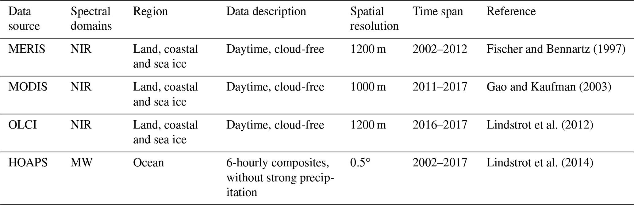
The TCWV is commonly defined as the vertically integrated water vapour over the full column with units of kilograms per square metre (kg m−2). Observations from microwave (MW) imagers (namely SSM/I, SSMIS, AMSR-E and TMI) over the ice-free ocean, partly based on a fundamental CDR (Fennig et al., 2020), and near-infrared (NIR) imagers (including MERIS, MODIS-Terra and OLCI) over land, coastal ocean and sea ice have been combined within the ESA CCI_WV project. Details of the retrieval are discussed in Andersson et al. (2010) and Schröder et al. (2013) for the MW imagers. The algorithms for NIR imagers are discussed in Lindstrot et al. (2012), Diedrich et al. (2015) and Preusker et al. (2021). The MW and NIR data streams are processed independently and combined afterwards so that the individual TCWV values and their uncertainties remain unchanged. Validation of the dataset against GRUAN and SuomiNet shows that the bias and corrected RMSD (cRMSD) are generally small and within ±1.5 and 2.5 kg m−2, respectively. The available spatial resolutions of the combined data record (hereafter TCWV-COMBI) are 0.5∘ × 0.5∘ and 0.05∘ × 0.05∘, where the NIR based data are averaged and the MW-based data are oversampled to produce the results with desired resolution. The daily and monthly mean data are available for the TCWV-COMBI product during July 2002–December 2017. Table 1 summarizes the various original data sources that are used in the TCWV-COMBI CDR.
Fischer and Bennartz (1997)Gao and Kaufman (2003)Lindstrot et al. (2012)Lindstrot et al. (2014)Table 1Summary of the characteristics of CCI water vapour data TCWV-COMBI.
Here we use the daily 0.05∘ × 0.05∘ TCWV-COMBI dataset. However, as detailed above, the data processing of the TCWV-COMBI is different between land and ocean, which then impacts the processing of the CMIP6 models: over land areas, TCWV is estimated under cloud-free conditions, while over ocean areas, TCWV is estimated until heavy precipitation occurs. Moreover the evaluation period is restricted to before 2014 for consistency with the available period of the CMIP6 experiment. Such a cut in the ESA TCWV-COMBI product excludes the OLCI observations.
2.2 CMIP6 models
Seven GCMs participating in CMIP6 are evaluated here, limited by the availability of the required geophysical variables at daily resolution (at least) that is comparable with the CCI_WV CDRs. However, there was no TCWV field at the daily frequency that was available from the Earth System Grid Federation (ESGF) (node of Institut Pierre Simon Laplace, IPSL). Therefore we recomputed TCWV from the vertical profiles of specific humidity q (in g kg−1) that were provided at the model vertical resolution. High vertical resolution of specific humidity (more than 19 vertical levels in the troposphere) was then necessary to be certain to capture the full tropospheric water vapour (using the extraction on a selection of pressure levels would bias the computation of TCWV).
The TCWV (in kg m−2) from each model is thus calculated using
where g is the gravitational acceleration constant, and dp is the difference between adjacent pressure levels (hPa).
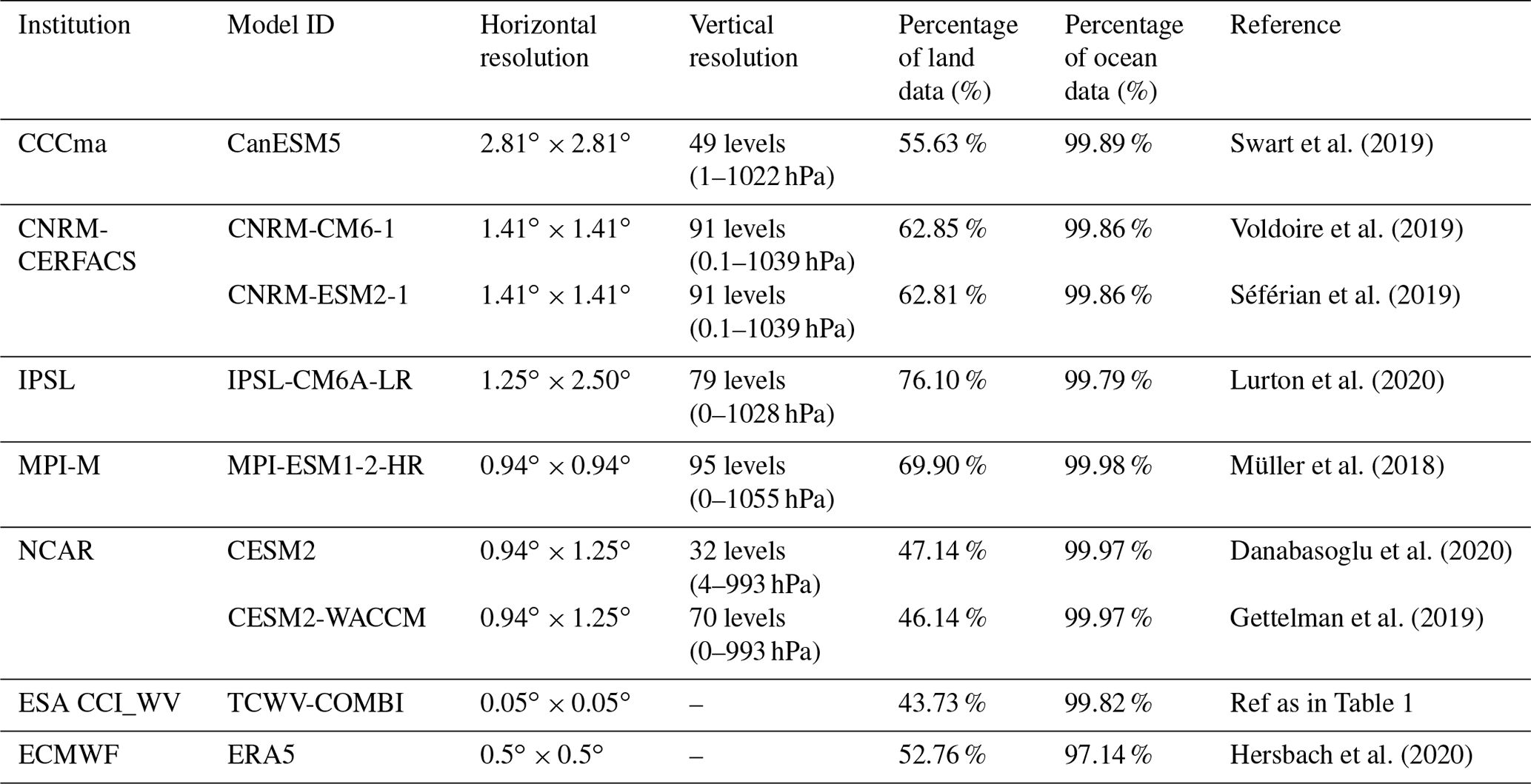
We focus on the AMIP (Atmospheric Model Inter-comparison Project) (Ackerley et al., 2018) scenario with prescribed time-varying sea surface temperature (SST) and sea-ice concentrations from observations, including variations in natural and anthropogenic external forcings (Eyring et al., 2016). The detailed model descriptions are listed in Table 2. In addition to the CMIP6 models, the ensemble mean of the seven models is also included in the following analysis to represent the mean state of the CMIP6 models.
Swart et al. (2019)Voldoire et al. (2019)Séférian et al. (2019)Lurton et al. (2020)Müller et al. (2018)Danabasoglu et al. (2020)Gettelman et al. (2019)Hersbach et al. (2020)Table 2Main characteristics of the seven CMIP6 models of the study, along with TCWV-COMBI and ERA5. The percentages over land and ocean are computed once the scene selection is applied.
Since the TCWV-COMBI data are cloud-screened over the land area, it is important to carefully analyse the cloud conditions for CMIP6 models before making the quantitative comparison. The cloud screening of the model-to-observation approach must remove the cloudy pixels while maintaining enough data for further evaluation. Since cloud fraction (cf) is the only parameter that is available for the CMIP6 models to be employed as the indicator for cloudiness, a series of threshold tests were conducted by screening the pixels with cf values larger than 5 %, 25 %, 50 % and 75 % at all pressure levels. The distribution of TCWV over tropical land from CanESM5 of the CMIP6 model with different cloud masks, along with data from TCWV-COMBI and ERA5, is shown in Fig. 1. The land area fraction product is adopted as the land–sea mask for the CanESM5 model. Here we defined the area as land where the percentage of the grid cell occupied by land is larger than 50 %. The results indicate that data with cf less than 50 % at all pressure levels show a reasonable spatial coverage comparable to TCWV-COMBI and ERA5. Therefore, this threshold is adopted as the general cloud mask for the CMIP6 models, although this cannot be considered a purely clear sky. It is worth mentioning that since the results are dependent on the cloud masks, the normalization process is also included in the following analysis to better illustrate the time evolution with respect to the mean state instead of strict biases.
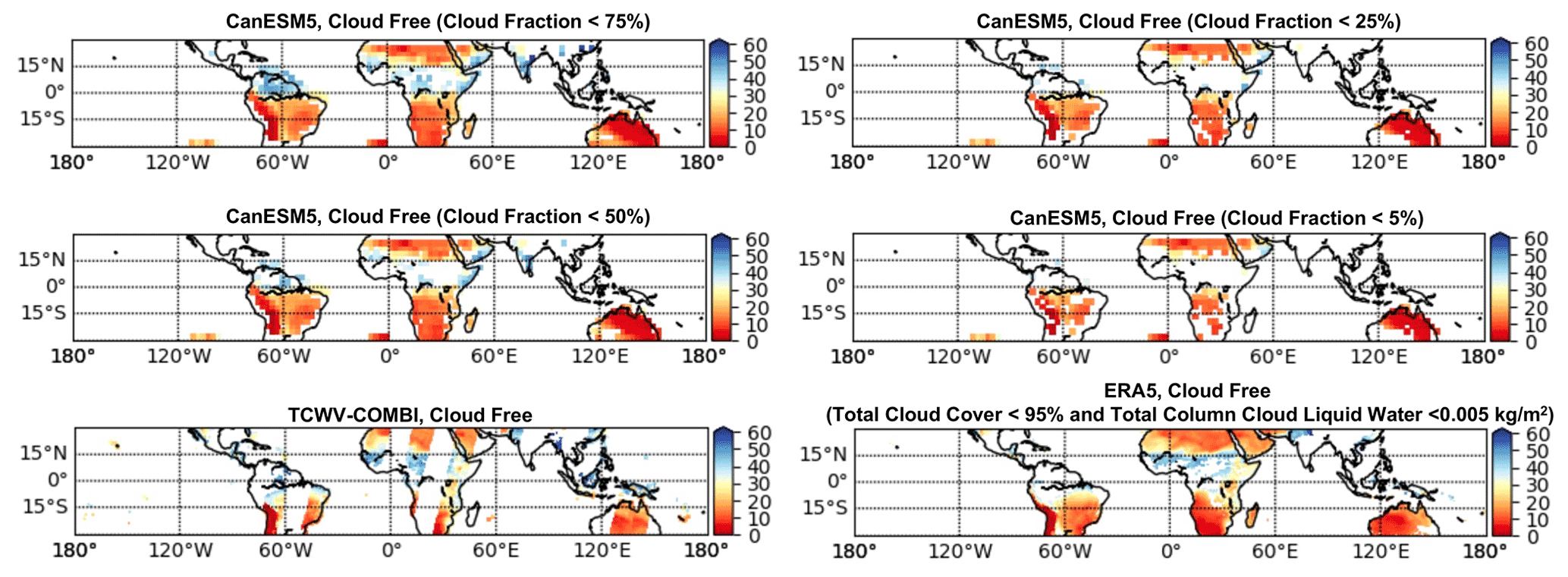
Figure 1Examples of daily mean TCWV over tropical land obtained from CanESM5 with different cloud mask (pixels with cloud fraction larger than 75 %, 50 %, 25 % and 5 % at all pressure levels are considered clouded), along with data from TCWV-COMBI and ERA5 from 1 July 2003.
The description of the datasets remaining for the following analysis after the cloud screening over the land and ocean is displayed in Table 2. Over land, the percentage of data that remained for the CMIP6 models after the cloud screening is globally in the range 46.14 %–76.10 %. Over tropical oceans, the percentage of data that remained after removing the pixels under heavy precipitation conditions ranges from 99.79 % to 99.98 %. Although the scene selection is more stringent over land, this indicates that the CMIP6 data used in the following analysis are comparable in terms of size of sample to the data from TCWV-COMBI and ERA5. It is worth mentioning that although the screening thresholds for the models are set to meet the criteria of the TCWV-COMBI product, the number of data retained for the comparison are not exactly the same for all models. Therefore, differences among datasets may be observed in the analysis. This is particularly true over tropical land.
2.3 ERA5
The reanalysis data are widely analysed in atmospheric sciences to assess the impact of changes in observation system, to scale progress in model simulations and to calculate climatology for forecast-error evaluation (Hersbach et al., 2020). The ECMWF's ERA5 TCWV data are based on the integrated forecasting system (IFS) Cy41r2, with considerably enhanced horizontal resolution of 31 km compared to 80 km for ERA-Interim. Here, the ERA5 TCWV data with hourly frequency are averaged into daily data. To compare the data under the same conditions, the ERA5 land–sea mask is employed for land and ocean separation, and a scene selection is performed and is similar to the process of the CMIP6 data. Hence, data with total cloud cover less than 95 % and total column cloud liquid water less than 0.005 kg m−2 over land (Sohn and Bennartz, 2008) and data with total precipitation less than 0.001 kg m−2 s−2 over ocean are retained.
The time series of the daily means of the CMIP6, ERA5 and ESA CCI_WV TCWV-COMBI are analysed with tropical-land and tropical-ocean separation over the common observation period that covers July 2003 to December 2014.
The intercomparisons are conducted according to two approaches.
-
The first approach evaluates the interannual variation of TCWV based on the probability distribution function (PDF) established from the daily records for each year of the period. The percentiles of the TCWV are defined from the yearly distributions, and the data are sorted by intervals of 10 percentiles. Finally, the mean TCWV of each interval is computed and normalized by the corresponding mean TCWV of the whole observation period for this given percentile.This is generalized for every percentile. This approach is meant to highlight the tropical anomalies with respect to the mean and trace back to the inter-annual variability of the tropical atmosphere.
-
The second approach is based on the fact that the water vapour distribution is strongly controlled by the large-scale vertical motion of the atmosphere. Therefore, we can use the mid-tropospheric atmospheric vertical velocity at 500 hPa (noted ω500 in hPa d−1) as a proxy for the vertical motions in the tropics (Bony et al., 2004). While such framework has been greatly used to study tropical clouds and their distribution (e.g., Konsta et al., 2012; Höjgård-Olsen et al., 2020), this link between vertical motion and TCWV is documented (e.g., Brogniez and Pierrehumbert, 2007) and further illustrated on Fig. 2. Figure 2 presents the TCWV-COMBI averaged over the whole 2003–2014 period as well as the mean winter (December, January and February – DJF) and mean summer (June, July and August – JJA), together with the corresponding ω500 taken from ERA5 at a monthly scale. As expected, a moist troposphere is associated with large-scale ascending motion (ω500 < 0 hPa d−1), while a dry troposphere is associated with large-scale subsidence (ω500 > 0 hPa d−1). The TCWV data are sorted upon 10 hPa d−1 bins of monthly values of ω500. The dynamical decomposition is performed for all TCWV data records for each year of the time period. Moreover, the TCWV data averaged over the whole 2003–2014 period are also sorted into the corresponding ω500 bins of the period, and this value is considered the reference to normalize the results. This second approach allows us to study the trends in TCWV for a given state of the large-scale dynamics and thus overcome issues associated with variations (such as shifts or expansion) of the atmospheric circulation (Vallis et al., 2015; Mbengue and Schneider, 2017).
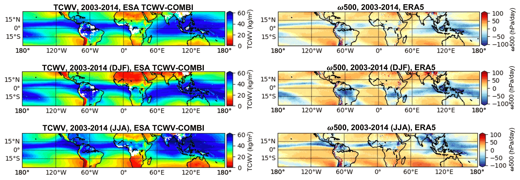
Figure 2Maps of the TCWV-COMBI (in kg m−2) during 2003–2014 for the tropical region (30∘ S–30∘ N) for the whole period, winter (December, January and February – DJF) and summer (June, July and August – JJA) and the corresponding maps of ERA5 ω500 (in hPa d−1).
This section aims to assess the degree of agreement in the TCWV climatology and interannual variations between the ESA CCI_WV TCWV-COMBI, CMIP6 models and ERA5 reanalysis data over the tropics (30∘ S–30∘ N). The distribution of the water vapour over tropics and its link to large-scale circulation (ω500) are discussed in detail.
4.1 Description of the tropical TCWV: 2003–2014
4.1.1 Time series
Figure 3 shows the time series of the TCWV of the different datasets over land (Fig. 3a; clear skies only) and over ocean (Fig. 3b; all weather without heavy precipitation) for the period July 2003–December 2014. There are differences in the range of daily mean TCWV, but all datasets varied with the seasons. Overall, the different data records agree well with each other despite some outliers observed over tropical land in TCWV-COMBI data that resulted from the differences in available sample size under the clear-sky condition each day. Strong seasonal variations are observed over tropical land with minima reached during JFM and maxima reached during JJA and with a very weak interannual variability. Since the results are dependent on the cloud-screening process, the detailed discussions on the impact of El Niño–Southern Oscillation (ENSO) events are discussed in Sect. 4.2. Over the tropical oceans, the seasonal variations are weaker (the minima still occur during JFM, but the maxima are not always reached in JJA) with a strong interannual variability.
More specifically, the ESA TCWV-COMBI data are moister than ERA5 and most CMIP6 models over both the land and the ocean areas, and this moist bias is even more pronounced over tropical land (Fig. 3a, ∼ 10 kg m−2 over land vs. ∼ 2 kg m−2 over ocean). On the other hand, the daily mean values of water vapour concentration over ocean areas are higher than the values over land areas. This difference can be explained because the TCWV datasets over land areas are composed of clear-sky-only data, which are likely drier than the nearby cloud area for a given location, thus translating into a dry bias associated with moistening processes by convective clouds (Sohn et al., 2006). Hence, the cloud screening over land makes it difficult to compare the datasets directly. In addition, since the boundary layer is drier in the continental subtropics and the maritime stratocumulus zones are wetter at low levels, the ocean areas should appear moister than the land areas.
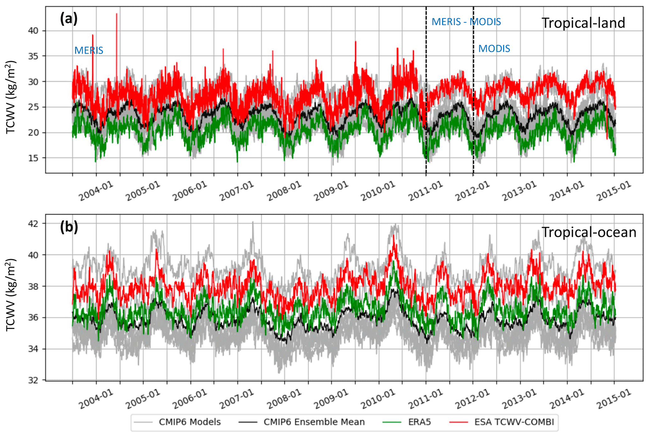
Figure 3Time series of daily mean TCWV in the tropics (30∘ S–30∘ N) over (a) land areas under clear-sky conditions and (b) ocean areas except for heavy precipitation (see details in Sect. 2). The time series cover the period July 2003–December 2014. The grey lines denote the individual CMIP6 models, while the black line represents their ensemble mean. The green line represents ERA5, and the red line is the ESA CCI_WV TCWV-COMBI.
4.1.2 The distribution of tropical TCWV
The normalized PDFs of the daily TCWV obtained from all data records over both land and ocean are displayed in Fig. 4. The bimodal distributions can be explained by the presence of more humid columns in the intertropical convergence zone (ITCZ) and relatively drier ones in subtropical regions. Similar to the time series analysis, the characteristics over land are significantly different to the results over the ocean area because of the data screening. Over land, all datasets reach a first maximum at around 10–13 kg m−2 and present a secondary maximum near 40–50 kg m−2. Moreover, more lower values are observed in the CMIP6 models and ERA5 than in the ESA TCWV-COMBI dataset, and this cannot be explained by the cloud-screening method alone. Indeed, the results of simulation models and ERA5 are dependent on cloud conditions, consequently leading to differences in the comparison. Although there are changes in variability in TCWV-COMBI data over tropical land with the inclusion of MODIS from 2011, validation of the dataset against GRUAN and SuomiNet shows that the dataset is stable and accurate during the whole observation period.
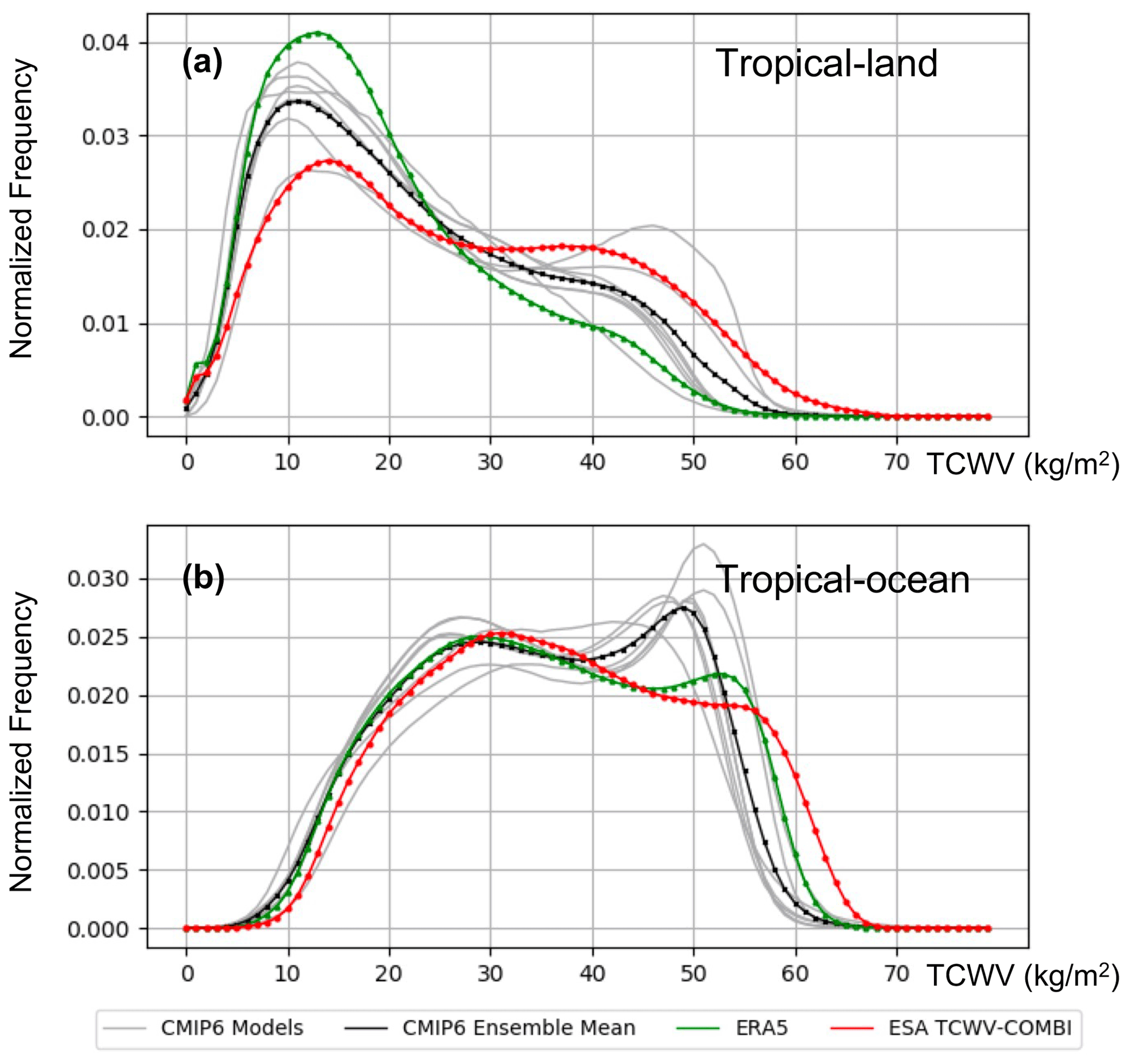
Figure 4The normalized PDFs of the TCWV in the tropical area (30∘ S–30∘ N) over (a) land areas (under clear-sky-only conditions) and over (b) ocean areas (under all-weather conditions except for heavy precipitation). The grey lines denote the individual CMIP6 models, while the black line represents their ensemble mean. The green line represents ERA5, and the red line is the ESA CCI+ TCWV-COMBI.
Over oceans, most of the TCWV data are located around 20–60 kg m−2. The main peak is around 30 kg m−2, and a secondary peak appears near 50 kg m−2. While the mean peak of PDF is nearly identical for TCWV-COMBI, ERA5 and CMIP6, there is a divergence for the secondary peak. This secondary peak even dominates the PDF of the CMIP6 models, while ERA5 and ESA TCWV-COMBI are still quite similar.
4.1.3 Extremes of the distributions
The data records are then evaluated following the approach (1) described in Sect. 3: the percentiles of the annual distributions of TCWV (at daily resolutions) are sorted into bins of 10 % intervals, and this is done for each year of the period.
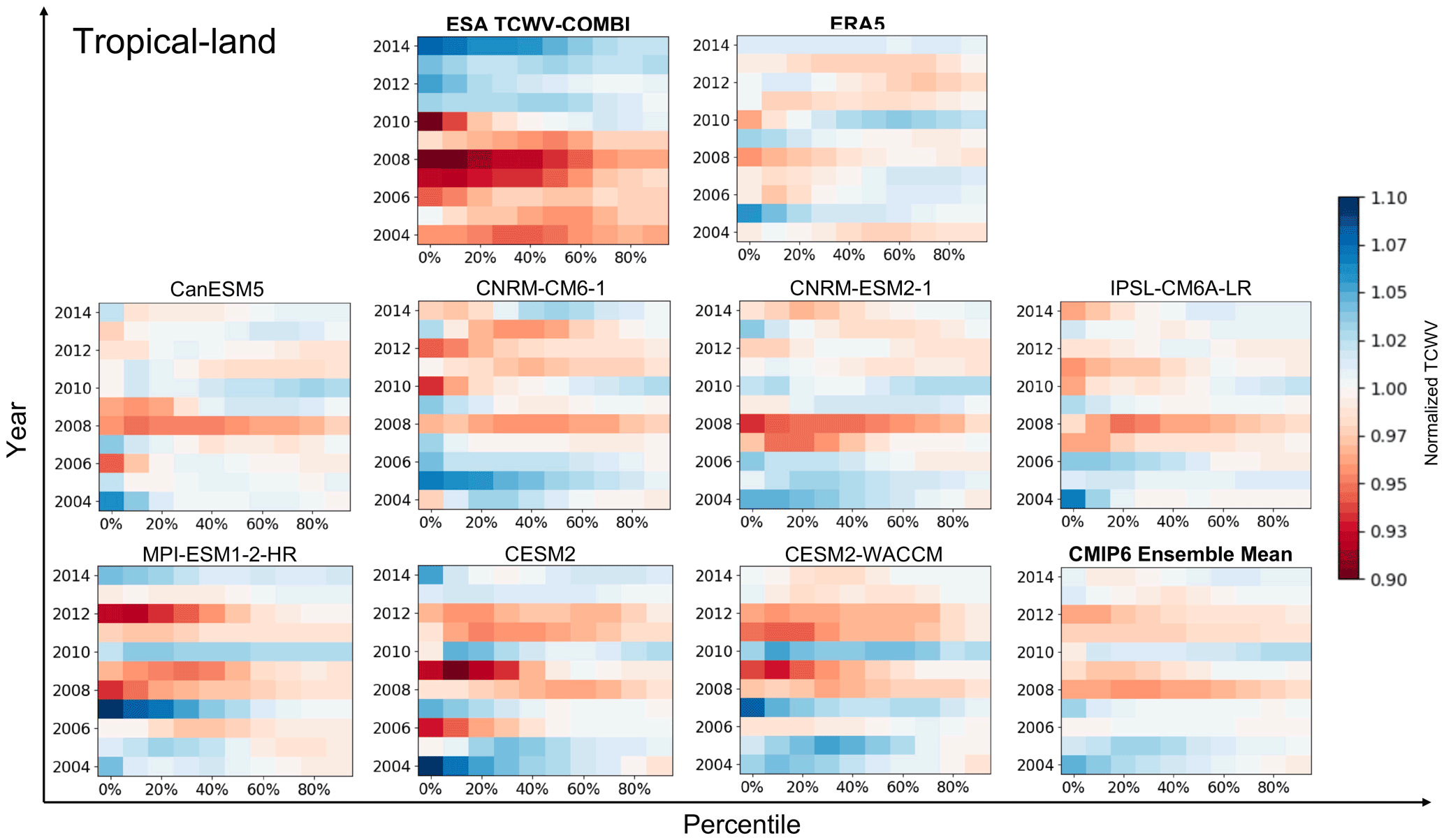
Figure 5Normalized percentiles of the TCWV over land areas for every data record. The percentiles are grouped into bins of 10 % intervals. The x axis represents the percentiles intervals, and the y axis represents the year. Note that the period starts in 2004 instead of 2003 to focus on full years.
The normalized TCWV for land areas and sorted by 10 percentile intervals for each year is displayed in Fig. 5. The bluish colours indicate that the TCWV value of the interval is larger than the reference value, indicating wet anomalies. The reddish colours indicate that the TCWV value is smaller than the reference, indicating dry anomalies. As shown in the figure, the ESA TCWV-COMBI data have quite different characteristics compared to CMIP6 and ERA5 results. A clear moistening trend is observed in the drier percentiles of TCWV-COMBI record. The tipping point seems to be 2011 and thus may be caused by the inhomogeneity of cloud-mask products for different observation instruments when computing the ESA TCWV-COMBI data. Indeed, the data record merged NIR observation from MERIS over 2002–2012, and MODIS observations are included over 2011–2017. Despite individual discrepancies, the CMIP6 ensemble mean is in good agreement with the ERA5 data. Overall, anomalies are observed in the time period for all data records: 2008 appears to be a dry year, while 2010 reveals a clear signal of humidification, especially over the high parts of the distributions of TCWV (percentiles > 60 %).
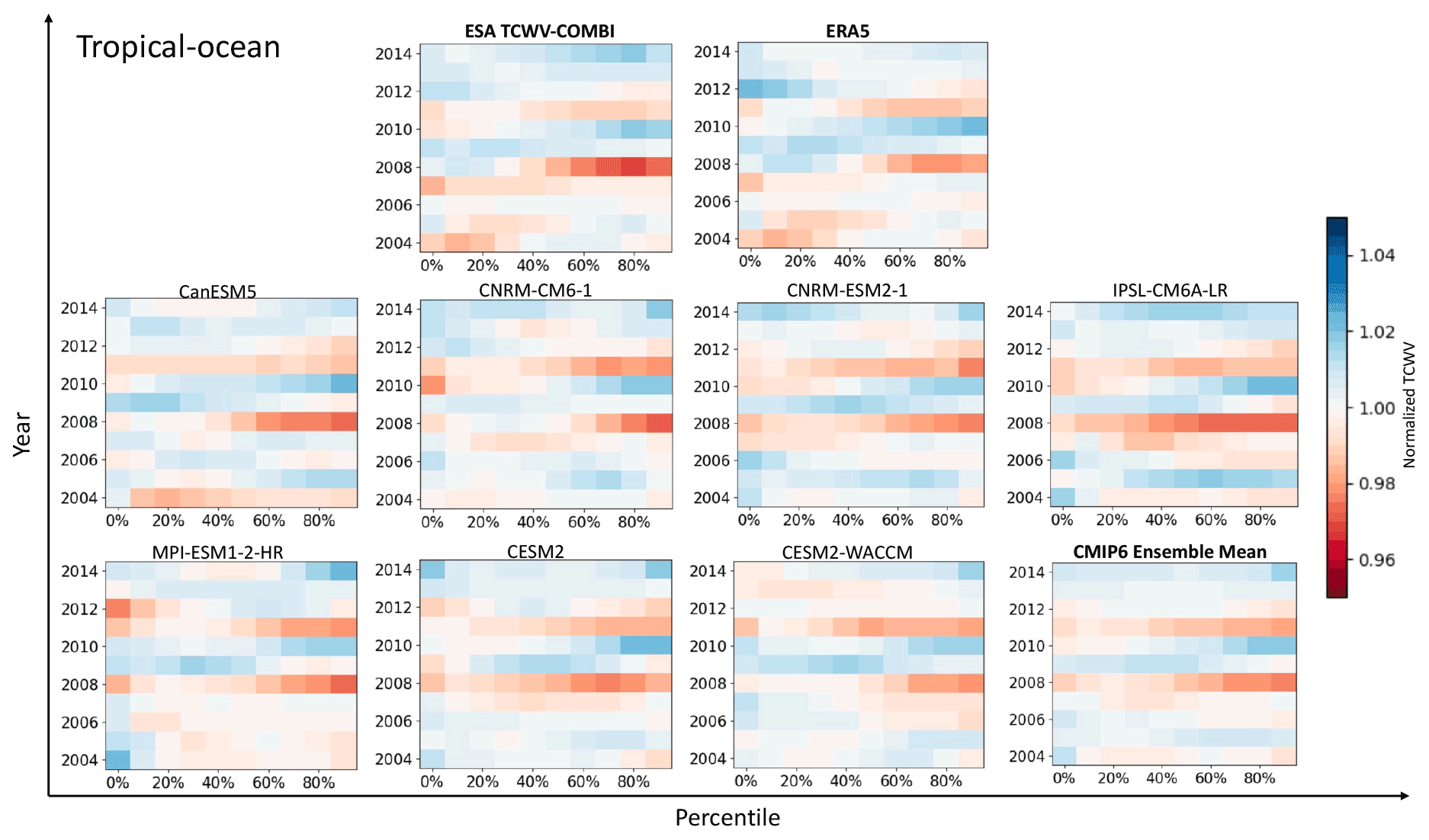
A similar comparison is performed over the tropical oceans, and the results are shown in Fig. 6. The TCWV-COMBI results coincided well with CMIP6 models and ERA5 data. Dry anomalies are observed in 2004 for the ESA TCWV-COMBI and ERA5 in the dry end of TCWV. Dry anomalies are also observed in 2008 and 2011 over the highest percentiles (>60 %) for all data records, while 2008 is the driest year of the period. Wet anomalies are observed in 2010 for the highest percentiles in all data records. ERA5 also reveals 2012 as a moister year, in the low range of TCWV, but this anomalous year is not present in the ESA TCWV-COMBI or CMIP6 ensemble mean. The very good agreement among the various datasets is largely due to the fact that the CMIP6 models are evaluated under the AMIP scenario, so with the same prescribed SST for all models and ERA5, and that the relationship between SST and TCWV is largely explained by the Clausius–Clapeyron law (Stephens, 1990). Hence this explains that anomalous years are the results of El Niño–Southern Oscillation (Trenberth et al., 2005): 2008 and 2011 are characterized by a very negative ENSO index, while 2010 is an intermediate year, which starts with a positive ENSO cycle and is followed by a negative one.
4.2 TCWV and large-scale circulation
4.2.1 General assessment
The interannual variability of TCWV is then analysed from its links with the large-scale atmospheric circulation and follows approach (2) described in Sect. 3. The monthly ω500 of individual data records is decomposed into intervals of 10 hPa d−1 in the range of −120 to 120 hPa d−1. Figure 7 displays the normalized PDFs of the ω500 of the CMIP6 models and ERA5. As mentioned earlier, there are no atmospheric circulation data from the ESA TCWV-COMBI data record, so the ω500 from ERA5 is also employed as the reference for this dataset. Figure 7a and b show that the PDFs of the ω500 from the CMIP6 ensemble mean agree well with the ERA5 data. Most of the ω500 reside in around 10–20 hPa d−1 over both the tropical-land and tropical-ocean area, which characterizes the dominance of the large-scale Hadley subsidence in the subtropical free troposphere and explains the clear-sky radiative cooling of the tropics as discussed in Bony et al. (2004).

Figure 7(a, b) Normalized PDFs of ω500 (in hPa d−1) over land (a) and ocean (b) for CMIP6 models (grey lines), their ensemble mean (black line) and ERA5 (green line). (c, d) Mean TCWV from the CMIP6 models (grey lines), their ensemble mean (black line), ERA5 (green line) and ESA TCWV-COMBI (red line) in different circulation regimes of ω500 over land (c) and ocean (d) areas. The shaded area in pink represents the σ of each bin in TCWV-COMBI data.
The TCWV of each dataset is then sorted into the vertical velocity bins by the corresponding value of ω500. Therefore, the variations of the TCWV can be analysed from the perspective of atmospheric vertical motion. As shown in Fig. 7c and d, large-scale downward motion is associated with a dry troposphere, while large-scale ascent is associated with a moister troposphere (except for ERA5 over land, where the most humid regimes are over weak subsidence). The results are in agreement with the maps of Fig. 2. Overall, the CMIP6 models and ERA5 show differences with the ESA TCWV-COMBI data in the amplitude of the signal and in the gradient of moisture between the ascending and descending regions. The evaporation from the oceans is the primary source of water vapour in the atmosphere; the oceanic boundary layer is humid, even in a weak subsidence regime. Further, as the reference ω500 for TCWV-COMBI is from ERA5, it is sensible that there are differences observed in the TCWV-COMBI data comparing to other datasets that are decomposed by the corresponding model products. While the large-scale atmospheric dynamics are consistent among the datasets, the discrepancies in the TCWV reveal difficulties in representing the moistening processes of the tropical atmosphere: lateral mixing (Pierrehumbert and Roca, 1998; Pierrehumbert, 1998), outflows from clouds and too high/too low precipitation efficiencies of the convective schemes (Brogniez and Pierrehumbert, 2007). It is worth mentioning that the moistest regime of TCWV from ERA5 over land areas occurred in a weak subsidence regime instead of the strong ascending region. This difference is partly because of the cloud-screening processes. Therefore, the results could not accurately represent the large-scale advection humidification/drying processes.
4.2.2 Trends over lands
This global assessment is further discussed by applying the TCWV–ω500 approach for every year of each data record to delineate the trends in TCWV. As shown in Fig. 8, all the data records (except for ERA5) agree that the driest troposphere (red) is associated with the most positive ω500 bins (meaning the areas of highest downward motion). The moistest troposphere, however, is not always located in the most negative ω500 bins (the highest upward motion).
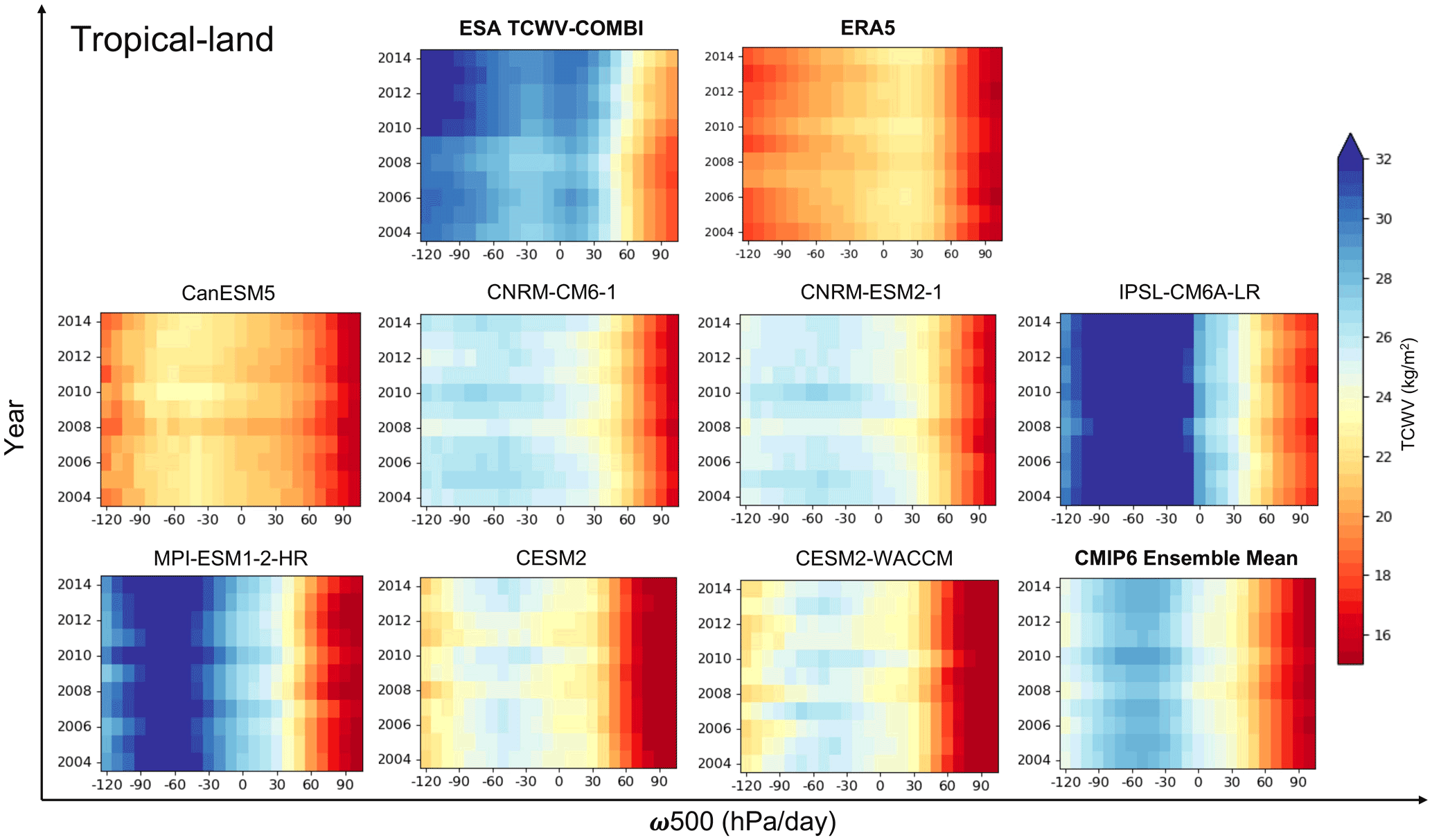
Figure 8Mean of TCWV over tropical-land areas at each dynamical interval (ω500) in 10 hPa d−1 computed from each data record.
ERA5 and the CMIP6 ensemble mean display the lowest TCWV values (< 16 kg m−2) that occur all along the 2004–2014 period, while the ESA TCWV-COMBI data record reaches values ∼ 18 kg m−2, and this minimum is reached over 2007–2008. There is also a very strong variability amongst the CMIP6 models: IPSL-CM6A-LR is clearly the moistest model, and CanESM5 is the driest. The moist bias of IPSL-CM6A-LR is already documented (Boucher et al., 2020) and is explained by the (too) efficient parametrization scheme of the transport of evaporated air from the surface to the top of the boundary layer. The discrepancy observed from CanESM5 is partly because of its strong effective climate efficiency compared to other CMIP6 models (Virgin et al., 2021). For the CanESM5, the positive low and non-low shortwave cloud feedbacks, as well as subtropical and extratropical free troposphere cloud optical depth, particularly with regards to low clouds across the equatorial Pacific, are the dominant contributors to its increased climate sensitivity (Virgin et al., 2021). ERA5 also displays a very dry troposphere in all dynamical regimes.
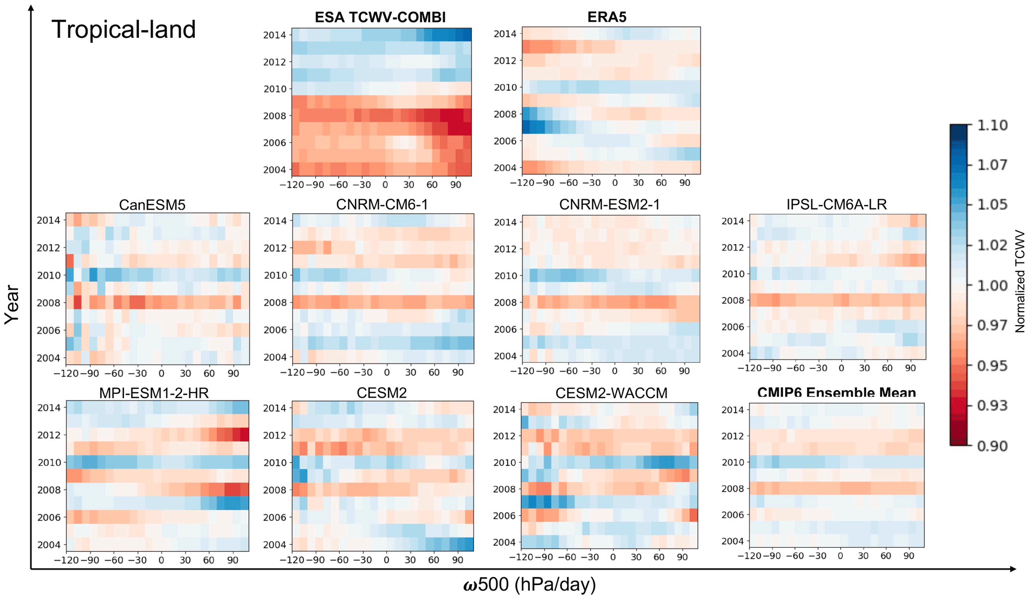
Figure 9Normalized TCWV with respect to the 2004–2014 mean over tropical-land areas at each dynamical interval (ω500) in 10 hPa d−1 computed from each data record.
To unravel the anomalies of TCWV, the mean values of TCWV of each circulation regime observed during the whole comparison period (2004–2014) are employed as the reference to normalize the results. The normalized TCWV at each circulation interval for the different data records is displayed in Fig. 9. Although different patterns are observed, dry anomalies occurred in 2008 in all of the data records (except for ERA5, Du et al., 2021, where dry anomalies were observed for subsidence and weak upward motion regimes), and wet anomalies occurred in 2010. These extreme years are consistent with the previous findings (Sect. 4.1.3), and this second approach provides another angle of analysis on the assessment.
-
The ESA TCWV-COMBI reveals a clear moistening tendency, especially over the subsiding branch of the atmospheric circulation after 2011. One of the major causes of the turning point is the inclusion of MODIS data from 2011, which would increase the sampling size of the data and in turn affect the tendency.
-
The TCWV from ERA5 shows only extreme years but no distinct tendency. In the regions of highest upward motions, 2007 and 2008 appear moister than the other years, while 2004 and 2013 appear drier. Once again, this may be due to the scene selection applied over land, but this would not entirely explain the differences with the ESA TCWV-COMBI.
-
Finally, the CMIP6 models and their ensemble mean show consistent interannual variabilities: dry anomalies occurred in 2008 in all the data records, and wet anomalies occurred in 2010. The results of the models are in a relative agreement with ERA5 and ESA TCWV-COMBI.
4.2.3 Trends over oceans
Oceanic situations were also discussed with respect to the large-scale circulation. The results are shown in Fig. 10 (mean TCWV) and Fig. 11 (normalized TCWV). As the data over ocean areas are obtained under all-weather conditions except for heavy precipitation, the impacts from clear-sky biases are greatly reduced. All data records, except for TCWV-COMBI, CanESM5 and IPSL-CM6A-LR, show that the strongest ascending zones correspond to the very humid regions. Different from the results over land, where the CMIP6 models showed strong differences (CanESM5 was the driest, and IPSL-CM6A-LR was the moistest), the amplitudes and gradients of moisture are closer to each other over oceans. Since the transport model in the boundary layer of IPSL-CM6A-LR affects both shallow and deep convection regimes, a compensational bias would be induced; thus a moist bias will be present in the weak upward motion regimes ( hPa d−1) (Boucher et al., 2020). The normalized TCWV with respect to dynamical intervals over ocean areas is shown in Fig. 11. The temporal evolutions of TCWV–ω500 are consistent with the earlier analysis based on the temporal evolution of the percentiles of TCWV over ocean (Sect. 4.1.3). The extremely dry and moist years (2008 and 2010 respectively) are the same between ESA TCWV-COMBI, ERA5 and the CMIP6 ensemble mean.
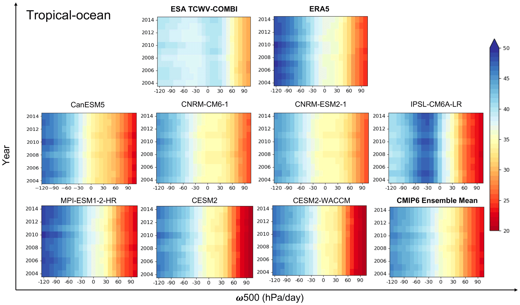
Figure 10Mean of TCWV over tropical-ocean areas at each dynamical interval (ω500) in 10 hPa d−1 computed from each data record.

Figure 11Normalized TCWV with respect to the 2004–2014 mean over tropical-ocean areas at each dynamical interval (ω500) in 10 hPa d−1 computed from each data record.
Despite the importance of water vapour in the study of climate variability, our ability to evaluate the water vapour feedback is constrained by its measurements at ranges of scales that are adapted for local, regional and global studies. This deficiency is attributable in part to the fact that it is difficult to quantitatively and accurately measure the distribution of water vapour. To work towards the requirement of GCOS on satellite-based water vapour observation as an ECV, the ESA Climate Change Initiative Water Vapour project (ESA CCI_WV) tackled this challenge by generating gridded products on stratospheric and tropospheric water vapour from multiple satellite observations suitable for climate and process studies.
We have conducted a comprehensive evaluation of the tropical water vapour (30∘ N–30∘ S) of seven GCMs (CMIP6 models, AMIP scenario) and ERA5, using the TCWV-COMBI climate data record developed within the ESA CCI_WV project as a reference. The study focused over tropical-land and tropical-ocean areas at the daily frequency and over the 2003–2014 period. The variability of TCWV was analysed according to (i) its probability density function (PDF) defined at a yearly scale over the period and to (ii) the large-scale circulation using the atmospheric vertical velocity at 500 hPa (ω500) as a proxy for the tropospheric overturning circulation.
Different patterns of variability are observed among the various datasets, the largest discrepancies being noticed over land areas, while over the oceans, the datasets are closer to each other.
-
Over land, the PDFs of the ESA TCWV-COMBI present a clear moistening trend of their driest percentiles, with a tipping point in 2011, probably associated with the addition of the MODIS observation in the climate data record. The projection of the TCWV onto regimes of ω500 shows the same behaviour; dry anomalies occurred in 2008 in all of the data records (except for ERA5, where dry anomalies were observed for subsidence and weak upward motion regimes), and wet anomalies occurred in 2010. Interestingly, the CMIP6 ensemble mean and the ERA5 reanalysis are in good agreement in terms of interannual anomalies, although the ERA5 TCWV is clearly too dry.
-
Over ocean, the PDFs of all datasets present the same interannual variability. The extremely dry and moist years, associated with El Niño and La Niña events, are the same. This similarities hold when using the large-scale circulation as an evaluation tool, with the same transition between the dry/subsiding regimes and the moister/ascending regimes.
The results show that the ESA TCWV-COMBI data and ERA5 data vary within the ensemble spread of CMIP6 models, indicating that the mean models could correctly represent the evolution of water vapour with respect to large-scale circulation. The humid area is related to the ascending motion (negative value in ω500), and the dry area is related to the subsiding motion (positive value in ω500) over both tropical-land and tropical-ocean areas. There are discrepancies observed among the data records, probably caused by the lateral mixing, outflows from clouds and the precipitation efficiencies of the convective schemes. It is difficult to track the reasons for the differences entirely; however, the differences and similarities can be explained by several factors.
-
The use of different satellites with different accuracies and resolutions within the ESA TCWV-COMBI may explain part of the moistening trend observed for this dataset over land.
-
The cloud masks applied to the GCMs and ERA5 and defined to mimic the cloud mask of the observation can also explain the differences.
-
The parametrization of the moisture fluxes at the surface and of convection, as well as the climate efficiency of the GCMs, also contributes to the observed differences.
-
The CMIP6 models under the AMIP scenario (with prescribed sea surface temperatures) and the scene selection that is much more conservative than over land explained the agreement between the ESA TCWV-COMBI, ERA5 and the GCMs over oceans.
It is really necessary to underline the role of the cloud mask in the assessment of water vapour fields in climate models using observations, even though it is easier to compare water vapour than clouds. The water vapour profiles (and sometimes the integrated values) from climate models usually have coarser spatial resolution than satellite observations. The satellite measurements, on the other hand, are often strictly restrained by cloud contamination. This clearly shows the importance of having access to the simulated water vapour (full profiles as well as integrated values) for the clear-sky part of the meshes of the climate models.
Code is available from the corresponding author upon request (jia.he@latmos.ipsl.fr).
The CMIP6 data are available from the ESGF system (https://esgf-node.ipsl.upmc.fr/projects/esgf-ipsl/, ESGF, 2022), and the CCI Water Vapour data are available from the project website (https://climate.esa.int/en/projects/water-vapour/, ESA, 2022).
JH carried out the data analysis and prepared all the figures. JH, HB and LP contributed to the interpretation of the results and wrote the paper.
The contact author has declared that none of the authors has any competing interests.
Publisher's note: Copernicus Publications remains neutral with regard to jurisdictional claims in published maps and institutional affiliations.
This article is part of the special issue “Analysis of atmospheric water vapour observations and their uncertainties for climate applications (ACP/AMT/ESSD/HESS inter-journal SI)”. It is not associated with a conference.
The study was funded by ESA via the Water_Vapour_CCI project of ESA's Climate Change Initiative (CCI). The combined microwave and near-infrared-imager-based product COMBI was initiated and funded by the ESA Water_Vapour_CCI project, with contributions from Brockmann Consult, Spectral Earth, Deutscher Wetterdienst and the EUMETSAT Satellite Climate Facility on Climate Monitoring (CM SAF). The combined MW and NIR product will be owned by EUMETSAT CM SAF and will be released by CM SAF in late 2021. This study benefited from the ESPRI (Ensemble de Services Pour la Recherche à l'IPSL) computing and data centre (https://mesocentre.ipsl.fr, last access: 19 September 2022).
This research has been supported by the European Space Agency (grant no. 4000123554).
This paper was edited by Martina Krämer and reviewed by three anonymous referees.
Ackerley, D., Chadwick, R., Dommenget, D., and Petrelli, P.: An ensemble of AMIP simulations with prescribed land surface temperatures, Geosci. Model Dev., 11, 3865–3881, https://doi.org/10.5194/gmd-11-3865-2018, 2018. a
Allan, R. P., Liu, C., Zahn, M., Lavers, D. A., Koukouvagias, E., and Bodas-Salcedo, A.: Physically consistent responses of the global atmospheric hydrological cycle in models and observations, Surv. Geophys., 35, 533–552, 2014. a
Allan, R. P., Barlow, M., Byrne, M. P., Cherchi, A., Douville, H., Fowler, H. J., Gan, T. Y., Pendergrass, A. G., Rosenfeld, D., Swann, A. L., Wilcox, L. J., and Zolina, O.: Advances in understanding large-scale responses of the water cycle to climate change, Ann. NY Acad. Sci., 1472, 49–75, 2020. a
Andersson, A., Fennig, K., Klepp, C., Bakan, S., Graßl, H., and Schulz, J.: The Hamburg Ocean Atmosphere Parameters and Fluxes from Satellite Data – HOAPS-3, Earth Syst. Sci. Data, 2, 215–234, https://doi.org/10.5194/essd-2-215-2010, 2010. a
Arias, P. A., Bellouin, N., Coppola, E., Jones, R. G., Krinner, G., Marotzke, J., Naik, V., Palmer, M. D., Plattner, G.-K., Rogelj, J., Rojas, M., Sillmann, J., Storelvmo, T., Thorne, P. W., Trewin, B., Achuta Rao, K., Adhikary, B., Allan, R. P., Armour, K., Bala, G., Barimalala, R., Berger, S., Canadell, J. G., Cassou, C., Cherchi, A., Collins, W., Collins, W. D., Connors, S. L., Corti, S., Cruz, F., Dentener, F. J., Dereczynski, C., Di Luca, A., Diongue Niang, A., Doblas-Reyes, F. J., Dosio, A., Douville, H., Engelbrecht, F., Eyring, V., Fischer, E., Forster, P., Fox-Kemper, B., Fuglestvedt, J. S., Fyfe, J. C., Gillett, N. P., Goldfarb, L., Gorodetskaya, I., Gutierrez, J. M., Hamdi, R., Hawkins, E., Hewitt, H. T., Hope, P., Islam, A. S., Jones, C., Kaufman, D. S., Kopp, R. E., Kosaka, Y., Kossin, J., Krakovska, S., Lee, J.-Y., Li, J., Mauritsen, T., Maycock, T. K., Meinshausen, M., Min, S.-K., Monteiro, P. M. S., Ngo-Duc, T., Otto, F., Pinto, I., Pirani, A., Raghavan, K., Ranasinghe, R., Ruane, A. C., Ruiz, L., Sallée, J.-B., Samset, B. H., Sathyendranath, S., Seneviratne, S. I., Sörensson, A. A., Szopa, S., Takayabu, I., Tréguier, A.-M., van den Hurk, B., Vautard, R., von Schuckmann, K., Zaehle, S., Zhang, X., and Zickfeld, K.: Technical Summary, in: Climate Change 2021: The Physical Science Basis. Contribution of Working Group I to the Sixth Assessment Report of the Intergovernmental Panel on Climate Change, edited by: Masson-Delmotte, V., Zhai, P., Pirani, A., Connors, S. L., Péan, C., Berger, S., Caud, N., Chen, Y., Goldfarb, L., Gomis, M. I., Huang, M., Leitzell, K., Lonnoy, E., Matthews, J. B. R., Maycock, T. K., Waterfield, T., Yelekçi, O., Yu, R., and Zhou, B., Cambridge University Press, Cambridge, United Kingdom and New York, NY, USA, 33−-144, 2021. a
Bony, S., Dufresne, J.-L., Le Treut, H., Morcrette, J.-J., and Senior, C.: On dynamic and thermodynamic components of cloud changes, Clim. Dynam., 22, 71–86, 2004. a, b, c, d
Boucher, O., Servonnat, J., Albright, A. L., Aumont, O., Balkanski, Y., Bastrikov, V., Bekki, S., Bonnet, R., Bony, S., Bopp, L., Braconnot, P., Brockmann, P., Cadule, P., Caubel, A., Cheruy, F., Codron, F., Cozic, A., Cugnet, D., D'Andrea, F., Davini, P., Casimir de Lavergne, Denvil, S., Deshayes, J., Devilliers, M., Ducharne, A., Dufresne, J. L., Dupont, E., Éthé, C., Fairhead, L., Falletti, L., Flavoni, S., Foujols, M. A., Gardoll, S., Gastineau, G., Ghattas, J., Grandpeix, J. Y., Guenet, B., Guez, L. E., Guilyardi, E., Guimberteau, M., Hauglustaine, D., Hourdin, F., Idelkadi, A., Joussaume, S., Kageyama, M., Khodri, M., Krinner, G., Lebas, N., Levavasseur, G., Lévy, C., Li, L., Lott, F., Lurton, T., Luyssaert, S., Madec, G., Madeleine, J. B., Maignan, F., Marchand, M., Marti, O., Mellul, L., Meurdesoif, Y., Mignot, J., Musat, I., Ottlé, C., Peylin, P., Planton, Y., Polcher, J., Rio, C., Rochetin, N., Rousset, C., Sepulchre, P., Sima, A., Swingedouw, D., Thiéblemont, R., Traore, A. K., Vancoppenolle, M., Vial, J., Vialard, J., Viovy, N., and Vuichard, N.: Presentation and evaluation of the IPSL-CM6A-LR climate model, J. Adv. Model. Earth Sy., 12, e2019MS002010, https://doi.org/10.1029/2019MS002010, 2020. a, b
Brogniez, H. and Pierrehumbert, R. T.: Intercomparison of tropical tropospheric humidity in GCMs with AMSU-B water vapor data, Geophys. Res. Lett., 34, L17812, https://doi.org/10.1029/2006GL029118, 2007. a, b
Chung, E.-S., Soden, B. J., Sohn, B.-J., and Schmetz, J.: Model-simulated humidity bias in the upper troposphere and its relation to the large-scale circulation, J. Geophys. Res.-Atmos., 116, D10110, https://doi.org/10.1029/2011JD015609, 2011. a
Belward, A. and Dowell, M. (Eds.): The Global Observing System for Climate: Implementation Needs, World Meteorological Organization (WMO), https://library.wmo.int/index.php?lvl=notice_display&id=19838#.Yyvvd-wzY6E (last access: 19 September 2022), 2016. a
Danabasoglu, G., Lamarque, J.-F., Bacmeister, J., Bailey, D., DuVivier, A., Edwards, J., Emmons, L., Fasullo, J., Garcia, R., Gettelman, A., Hannay, C., Holland, M. M., Large, W. G., Lauritzen, P. H., Laurence, D. M., Lenaerts, J. T. M., Lindsay, K., Lipscomb, W. H., Mills, M. J., Neale, R., Oleson, K. W., Otto-Bliesner, B., Phillips, A. S., Sacks, W., Tilmes, S., van Kampenhout, L., Vertenstein, M., Bertini, A., Dennis, J., Deser, C., Fischer, C., Fox-Kemper, B., Kay, J. E., Kinnison, D., Kushner, P. J., Larson, V. E., Long, M. C., Mickelson, S., Moore, J. K., Nienhouse, E., Polvani, L., Rasch, P. J., and Strand, W. G.: The community earth system model version 2 (CESM2), J. Adv. Model. Earth Sy., 12, e2019MS001916, https://doi.org/10.1029/2019MS001916, 2020. a
Diedrich, H., Preusker, R., Lindstrot, R., and Fischer, J.: Retrieval of daytime total columnar water vapour from MODIS measurements over land surfaces, Atmos. Meas. Tech., 8, 823–836, https://doi.org/10.5194/amt-8-823-2015, 2015. a
Du, M., Huang, K., Zhang, S., Huang, C., Gong, Y., and Yi, F.: Water vapor anomaly over the tropical western Pacific in El Niño winters from radiosonde and satellite observations and ERA5 reanalysis data, Atmos. Chem. Phys., 21, 13553–13569, https://doi.org/10.5194/acp-21-13553-2021, 2021. a
ESA: CCI water vapour data, ESA [data set], https://climate.esa.int/en/projects/water-vapour/, last access: 19 September 2022. a
ESGF: CMIP6, ESGF [data set], https://esgf-node.ipsl.upmc.fr/projects/esgf-ipsl/, last access: 19 September 2022. a
Eyring, V., Bony, S., Meehl, G. A., Senior, C. A., Stevens, B., Stouffer, R. J., and Taylor, K. E.: Overview of the Coupled Model Intercomparison Project Phase 6 (CMIP6) experimental design and organization, Geosci. Model Dev., 9, 1937–1958, https://doi.org/10.5194/gmd-9-1937-2016, 2016. a, b
Fennig, K., Schröder, M., Andersson, A., and Hollmann, R.: A Fundamental Climate Data Record of SMMR, SSM/I, and SSMIS brightness temperatures, Earth Syst. Sci. Data, 12, 647–681, https://doi.org/10.5194/essd-12-647-2020, 2020. a
Fischer, J. and Bennartz, R.: Retrieval of total water vapour content from MERIS measurements, Algorithm Theoretical Basis Document PO-TN-MEL-GS, 5, Institute for Space Sciences, Freie Universität Berlin, https://earth.esa.int/eogateway/instruments/meris/atbd (last access: 19 September 2022), 1997. a
Gao, B.-C. and Kaufman, Y. J.: Water vapor retrievals using Moderate Resolution Imaging Spectroradiometer (MODIS) near-infrared channels, J. Geophys. Res.-Atmos., 108, 4389, https://doi.org/10.1029/2002JD003023, 2003. a
Gettelman, A., Mills, M., Kinnison, D., Garcia, R., Smith, A., Marsh, D., Tilmes, S., Vitt, F., Bardeen, C., McInerny, J., Liu, H. L., Solomon, S. C., Polvani, L. M., Emmons, L. K., Lamarque, J. F., Richter, J. H., Glanville, A. S., Bacmeister, J. T., Phillips, A. S., Neale, R. B., Simpson, I. R., DuVivier, A. K., Hodzic, A., and Randel, W. J.: The whole atmosphere community climate model version 6 (WACCM6), J. Geophys. Res.-Atmos., 124, 12380–12403, https://doi.org/10.1029/2019JD030943, 2019. a
Held, I. M. and Soden, B. J.: Water vapor feedback and global warming, Annu. Rev. Energ. Env., 25, 441–475, 2000. a
Hersbach, H., Bell, B., Berrisford, P., Hirahara, S., Horányi, A., Muñoz-Sabater, J., Nicolas, J., Peubey, C., Radu, R., Schepers, D., Simmons, A., Soci, C., Abdalla, S., Abellan, X., Balsamo, G., Bechtold, P., Biavati, G., Bidlot, J., Bonavita, M., De Chiara, G., Dahlgren, P., Dee, D., Diamantakis, M., Dragani, R., Flemming, J., Forbes, R., Fuentes, M., Geer, A., Haimberger, L., Healy, S., Hogan, R.J., Hólm, E., Janisková, M., Keeley, S., Laloyaux, P., Lopez, P., Lupu, C., Radnoti, G., Patrica de Rosnay, Rozum, I., Vamborg, F., Villaume, S., and Thépaut, J. N.: The ERA5 global reanalysis, Q. J. Roy. Meteor. Soc., 146, 1999–2049, 2020. a, b
Höjgård-Olsen, E., Brogniez, H., and Chepfer, H.: Observed Evolution of the Tropical Atmospheric Water Cycle with Sea Surface Temperature, J. Climate, 33, 3449–3470, 2020. a, b
Huang, X., Soden, B. J., and Jackson, D. L.: Interannual co-variability of tropical temperature and humidity: A comparison of model, reanalysis data and satellite observation, Geophys. Res. Lett., 32, L17808, https://doi.org/10.1029/2005GL023375, 2005. a
IPCC (Hartmann, D. L., Klein Tank, A. M. G., Rusticucci, M., Alexander, L. V., Brönnimann, S., Charabi, Y., Dentener, F. J., Dlugokencky, E. J., Easterling, D. R., Kaplan, A., Soden, B. J., Thorne, P. W., Wild, M., and Zhai, P. M.): Observations: Atmosphere and Surface, in: Climate Change 2013: The Physical Science Basis. Contribution of Working Group I to the Fifth Assessment Report of the Intergovernmental Panel on Climate Change, edited by: Stocker, T. F., Qin, D., Plattner, G.-K., Tignor, M., Allen, S. K., Boschung, J., Nauels, A., Xia, Y., Bex, V., and Midgley, P. M., Cambridge University Press, Cambridge, United Kingdom and New York, NY, USA, https://www.ipcc.ch/report/ar5/wg1/ (last access: 24 September 2022), 2013. a
Jiang, J. H., Su, H., Zhai, C., Perun, V. S., Del Genio, A., Nazarenko, L. S., Donner, L. J., Horowitz, L., Seman, C., Cole, J., Gettelman, A., Ringer, M. A., Rotstayn, L., Jeffrey, S., Wu, T. W., Brient, F., Dufresne, J. L., Kawai, H., Koshiro, T., Watanabe, M., Lécuyer, T. S., Volodin, E. M., Iversen, T., Drange, H., Mesquita, M. D. S., Read, W. G., Waters, J. W., Tian, B. J., Teixeira, J., and Stephens, G. L.: Evaluation of cloud and water vapor simulations in CMIP5 climate models using NASA “A-Train” satellite observations, J. Geophys. Res.-Atmos., 117, D14105, https://doi.org/10.1029/2011JD017237. 2012. a
Konsta, D., Chepfer, H., and Dufresne, J.-L.: A process oriented characterization of tropical oceanic clouds for climate model evaluation, based on a statistical analysis of daytime A-train observations, Clim. Dynam., 39, 2091–2108, 2012. a
Lindstrot, R., Preusker, R., Diedrich, H., Doppler, L., Bennartz, R., and Fischer, J.: 1D-Var retrieval of daytime total columnar water vapour from MERIS measurements, Atmos. Meas. Tech., 5, 631–646, https://doi.org/10.5194/amt-5-631-2012, 2012. a, b
Lindstrot, R., Stengel, M., Schröder, M., Fischer, J., Preusker, R., Schneider, N., Steenbergen, T., and Bojkov, B. R.: A global climatology of total columnar water vapour from SSM/I and MERIS, Earth Syst. Sci. Data, 6, 221–233, https://doi.org/10.5194/essd-6-221-2014, 2014. a
Lu, J., Vecchi, G. A., and Reichler, T.: Expansion of the Hadley cell under global warming, Geophys. Res. Lett., 34, L06805, https://doi.org/10.1029/2006GL028443, 2007. a
Lurton, T., Balkanski, Y., Bastrikov, V., Bekki, S., Bopp, L., Braconnot, P., Brockmann, P., Cadule, P., Contoux, C., Cozic, A., Cugnet, D., Dufresne, J. L., Éthé, C., Foujols, M. A., Ghattas, J., Hauglustaine, D., Hu, R. M., Kageyama, M., Khodri, M., Lebas, N., Levavasseur, G., Marchand, M., Ottlé, C., Peylin, P., Sima, A., Szopa, S., Thiéblemont, R., Vuichard, N., and Boucher, O.: Implementation of the CMIP6 Forcing Data in the IPSL-CM6A-LR Model, J. Adv. Model. Earth Sy., 12, e2019MS001940, https://doi.org/10.1029/2019MS001940, 2020. a
Ma, J., Chadwick, R., Seo, K.-H., Dong, C., Huang, G., Foltz, G. R., and Jiang, J. H.: Responses of the tropical atmospheric circulation to climate change and connection to the hydrological cycle, Annu. Rev. Earth Pl. Sc., 46, 549–580, 2018. a
Mbengue, C. and Schneider, T.: Storm-track shifts under climate change: Toward a mechanistic understanding using baroclinic mean available potential energy, J. Atmos. Sci., 74, 93–110, 2017. a
Müller, W. A., Jungclaus, J. H., Mauritsen, T., Baehr, J., Bittner, M., Budich, R., Bunzel, F., Esch, M., Ghosh, R., Haak, H., Ilyina, T., Kleine, T., Kornblueh, L., Li, H., Modali, K., Notz, D., Pohlmann, H., Roeckner, E., Stemmler, I., Tian, F., and Marotzke, J.: A Higher-resolution Version of the Max Planck Institute Earth System Model (MPI-ESM1. 2-HR), J. Adv. Model. Earth Sy., 10, 1383–1413, https://doi.org/10.1029/2017MS001217, 2018. a
Pierrehumbert, R.: Lateral mixing as a source of subtropical water vapor, Geophys. Res. Lett., 25, 151–154, 1998. a
Pierrehumbert, R. T. and Roca, R.: Evidence for control of Atlantic subtropical humidity by large scale advection, Geophys. Res. Lett., 25, 4537–4540, 1998. a
Preusker, R., Carbajal Henken, C., and Fischer, J.: Retrieval of Daytime Total Column Water Vapour from OLCI Measurements over Land Surfaces, Remote Sensing, 13, 932, https://doi.org/10.3390/rs13050932, 2021. a
Raval, A. and Ramanathan, V.: Observational determination of the greenhouse effect, Nature, 342, 758–761, 1989. a
Schröder, M., Jonas, M., Lindau, R., Schulz, J., and Fennig, K.: The CM SAF SSM/I-based total column water vapour climate data record: methods and evaluation against re-analyses and satellite, Atmos. Meas. Tech., 6, 765–775, https://doi.org/10.5194/amt-6-765-2013, 2013. a
Schröder, M., Lockhoff, M., Shi, L., August, T., Bennartz, R., Brogniez, H., Calbet, X., Fell, F., Forsythe, J., Gambacorta, A., Ho, S. P., Kursinski, E. R., Reale, A., Trent, T., and Yang, Q.: The GEWEX water vapor assessment: Overview and introduction to results and recommendations, Remote Sensing, 11, 251, https://doi.org/10.3390/rs11030251, 2019. a
Séférian, R., Nabat, P., Michou, M., Saint-Martin, D., Voldoire, A., Colin, J., Decharme, B., Delire, C., Berthet, S., Chevallier, M., Sénési, S., Franchisteguy, L., Vial, J., Mallet, M., Joetzjer, E., Geoffroy, O., Guérémy, J. F., Moine, M. P., Msadek, R., Ribes, A., Rocher, M., Roehrig, R., Salas-y-Mélia, D., Sanchez, E., Terray, L., Valcke, S., Waldman, R., Aumont, O., Bopp, L., Deshayes, J., Éthé, C., and Madec, G.: Evaluation of CNRM Earth System Model, CNRM-ESM2-1: Role of Earth System Processes in Present-Day and Future Climate, J. Adv. Model. Earth Sy., 11, 4182–4227, https://doi.org/10.1029/2019MS001791, 2019. a
Sherwood, S., Roca, R., Weckwerth, T., and Andronova, N.: Tropospheric water vapor, convection, and climate, Rev. Geophys., 48, RG2001, https://doi.org/10.1029/2009RG000301, 2010. a
Sohn, B.-J. and Bennartz, R.: Contribution of water vapor to observational estimates of longwave cloud radiative forcing, J. Geophys. Res.-Atmos., 113, RG2001, https://doi.org/10.1029/2008JD010053, 2008. a
Sohn, B.-J., Schmetz, J., Stuhlmann, R., and Lee, J.-Y.: Dry bias in satellite-derived clear-sky water vapor and its contribution to longwave cloud radiative forcing, J. Climate, 19, 5570–5580, 2006. a
Stephens, G. L.: On the relationship between water vapor over the oceans and sea surface temperature, J. Climate, 3, 634–645, 1990. a
Swart, N. C., Cole, J. N. S., Kharin, V. V., Lazare, M., Scinocca, J. F., Gillett, N. P., Anstey, J., Arora, V., Christian, J. R., Hanna, S., Jiao, Y., Lee, W. G., Majaess, F., Saenko, O. A., Seiler, C., Seinen, C., Shao, A., Sigmond, M., Solheim, L., von Salzen, K., Yang, D., and Winter, B.: The Canadian Earth System Model version 5 (CanESM5.0.3), Geosci. Model Dev., 12, 4823–4873, https://doi.org/10.5194/gmd-12-4823-2019, 2019. a
Trenberth, K. E., Stepaniak, D. P., and Caron, J. M.: The global monsoon as seen through the divergent atmospheric circulation, J. Climate, 13, 3969–3993, 2000. a
Trenberth, K. E., Fasullo, J., and Smith, L.: Trends and variability in column-integrated atmospheric water vapor, Clim. Dynam., 24, 741–758, 2005. a
Vallis, G. K., Zurita-Gotor, P., Cairns, C., and Kidston, J.: Response of the large-scale structure of the atmosphere to global warming, Q. J. Roy. Meteor. Soc., 141, 1479–1501, 2015. a
Virgin, J. G., Fletcher, C. G., Cole, J. N. S., von Salzen, K., and Mitovski, T.: Cloud Feedbacks from CanESM2 to CanESM5.0 and their influence on climate sensitivity, Geosci. Model Dev., 14, 5355–5372, https://doi.org/10.5194/gmd-14-5355-2021, 2021. a, b
Voldoire, A., Saint-Martin, D., Sénési, S., Decharme, B., Alias, A., Chevallier, M., Colin, J., Guérémy, J.-F., Michou, M., Moine, M.-P., Nabat, P., Roehrig, R., Salas y Mélia, D., Séférian, R., Valcke, S., Beau, I., Belamari, S., Berthet, S., Cassou, C., Cattiaux, J., Deshayes, J., Douville, H., Ethé, C., Franchistéguy, L., Geoffroy, O., Lévy, C., Madec, G., Meurdesoif, Y., Msadek, R., Ribes, A., Sanchez-Gomez, E., Terray, L., and Waldman, R.: Evaluation of CMIP6 deck experiments with CNRM-CM6-1, J. Adv. Model. Earth Sy., 11, 2177–2213, https://doi.org/10.1029/2019MS001683, 2019. a
Wulfmeyer, V., Hardesty, R. M., Turner, D. D., Behrendt, A., Cadeddu, M. P., Di Girolamo, P., Schlüssel, P., Van Baelen, J., and Zus, F.: A review of the remote sensing of lower tropospheric thermodynamic profiles and its indispensable role for the understanding and the simulation of water and energy cycles, Rev. Geophys., 53, 819–895, 2015. a