the Creative Commons Attribution 4.0 License.
the Creative Commons Attribution 4.0 License.
 | 23 Sep 2022
Highly supercooled riming and unusual triple-frequency radar signatures over McMurdo Station, Antarctica
Frederic Tridon
Israel Silber
Alessandro Battaglia
Stefan Kneifel
Ann Fridlind
Petros Kalogeras
Ranvir Dhillon
Riming of ice crystals by supercooled water droplets is an efficient ice growth process, but its basic properties are still poorly known. While it has been shown to contribute significantly to surface precipitation at mid-latitudes, little is known about its occurrence at high latitudes. In Antarctica, two competing effects can influence the occurrence of riming: (i) the scarcity of supercooled liquid water clouds due to the extremely low tropospheric temperatures and (ii) the low aerosol concentration, which may lead to the formation of fewer and larger supercooled drops potentially resulting in an enhanced riming efficiency.
In this work, by exploiting the deployment of an unprecedented number of multiwavelength remote sensing systems (including triple-frequency radar measurements) in West Antarctica, during the Atmospheric Radiation Measurements West Antarctic Radiation Experiment (AWARE) field campaign, we evaluate the riming incidence at McMurdo Station and find that riming occurs at much lower temperatures when compared to previous results in the mid-latitudes. This suggests the possible occurrence of a common atmospheric state over Antarctica that includes a rather stable atmosphere inhibiting turbulent mixing, and a high riming efficiency driven by large cloud droplets.
We then focus on a peculiar case study featuring a persistent layer with a particularly pronounced riming signature in triple-frequency radar data but only a relatively modest amount of supercooled liquid water. In-depth analysis of the radar observations suggests that such signatures can only be explained by the combined effects of moderately rimed aggregates or similarly shaped florid polycrystals and a narrow particle size distribution (PSD). Simulations of this case study performed with a one-dimensional bin model indicate that similar triple-frequency radar observations can be reproduced when narrow PSDs are simulated. Such narrow PSDs can in turn be explained by two key factors: (i) the presence of a shallow homogeneous droplet or humidified aerosol freezing layer aloft seeding an underlying supercooled liquid layer, and (ii) the absence of turbulent mixing throughout a stable polar atmosphere that sustains narrow PSDs, as hydrometeors grow from the nucleation region aloft to ice particles of several millimeters in size, by vapor deposition and then riming.
- Article
(15051 KB) - Full-text XML
-
Supplement
(1014 KB) - BibTeX
- EndNote


Besides deposition and aggregation, riming is an efficient ice growth process. It contributes significantly to surface precipitation at mid-latitudes (Grazioli et al., 2015; Moisseev et al., 2017) and is pivotal for improving our understanding of the role of ice phase in the water budget. However, basic properties of riming such as its efficiency or its importance in precipitation formation are still largely unknown since it involves the collection of poorly characterized supercooled water droplets by complex ice particles. It is widely accepted, however, that at the beginning of a riming process, the mass of a rimed ice particle increases while its maximum dimension remains constant or increases only slightly (e.g., Heymsfield, 1982; Seifert et al., 2019); hence, the density and fall speed of rimed ice hydrometeors tend to be enhanced. Riming occurrence is strongly linked to temperature since the probability of finding supercooled liquid water decreases with temperature. By exploiting a multiyear dataset of cloud radar observations at four European sites in various environments, Kneifel and Moisseev (2020) showed that riming is rare below −12 ∘C and more frequent closer to 0 ∘C.
In the Arctic, supercooled liquid water clouds are frequent (e.g., Shupe et al., 2008; Cesana et al., 2012; Morrison et al., 2012; Mioche et al., 2015) and rimed precipitating particles are commonly observed (Mioche et al., 2017; Fitch and Garrett, 2022). In Antarctica, however, liquid water clouds are less frequent, in particular during winter months due to lower temperatures (e.g., Matus and L'Ecuyer, 2017; Lubin et al., 2020). Nevertheless, the typical low aerosol concentrations in this region can lead to the formation and persistence of supercooled drizzle drops (Silber et al., 2019a), which might facilitate the occurrence of riming due to the enhanced riming efficiency of drizzle drops (Lohmann, 2004). Therefore, a thorough investigation of riming in Antarctic clouds is timely.
Field measurements in Antarctica are historically sparse due to logistical challenges. Space-borne instruments such as the Cloud Profiling Radar (CPR) onboard CloudSat (Stephens et al., 2008) can cover extended and remote areas but have inherent limitations to measure weak ice precipitation fluxes (e.g., Silber et al., 2021), or any ice precipitation fluxes near the ground due to the so-called blind-zone (Maahn et al., 2014). Only recently, riming was shown to be a recurring process at an Antarctic site through ground-based optical probe observations at the Dumont d'Urville Station (Grazioli et al., 2017a), with most of the detected large ice hydrometeors being at least partially rimed. However, in order to detect an active riming process, suitable measurements are needed across the vertical column, which can be achieved via ground-based multifrequency radars, for example.
By analyzing scattering models of snow aggregates and graupel, Kneifel et al. (2011) suggested that triple-frequency radar measurements could be exploited to differentiate between rimed and unrimed ice particles. This differentiation was later verified by comparing triple-frequency radar signatures with bulk snow density derived from collocated ground-based observations (Kneifel et al., 2015). While the radar Doppler velocity is the simplest and most obvious parameter for retrieving the degree of riming or an equivalent parameter (e.g., density factor or rime mass fraction) of ice particles (e.g., Mosimann, 1995; Mason et al., 2018; Kneifel and Moisseev, 2020), triple-frequency radar observations can also provide critical information on the internal structure of snowflakes (Mason et al., 2019), and, hence, on the growth processes involved. For example, by exploiting triple-frequency Doppler spectra, Kneifel et al. (2016) combined triple-frequency and Doppler velocity information and confirmed that rimed and unrimed aggregates produce distinct scattering signatures. Further development of multifrequency radar retrievals demonstrated that the combination of three radar frequencies enables the derivation of snow aggregate properties with various degree of riming (e.g., Mason et al., 2018). Quantitative agreement was found with the measurements from collocated ground-based (Moisseev et al., 2017; von Lerber et al., 2017) or airborne (Leinonen et al., 2018; Tridon et al., 2019) in situ probes.
In the framework of the Atmospheric Radiation Measurement (ARM) West Antarctic Radiation Experiment (AWARE, Lubin et al., 2020), the U.S. Department of Energy (DOE) deployed the second ARM Mobile Facility (AMF2) at McMurdo Station from 1 December 2015 to 31 December 2016, resulting in an unprecedented suite of remote sensing instruments in Antarctica, including the Ka-band ARM Zenith Radar (KAZR), the Marine W-band ARM Cloud Radar (MWACR), and the scanning dual-wavelength ARM cloud radar system (X/KaSACR). Although the MWCAR stopped transmitting after about 3 months, these instruments provided triple-wavelength radar profiles for the first time in Antarctica (in Sect. 2). In this work, these data are exploited to evaluate the probability of finding triple-frequency signatures of riming in clouds over McMurdo Station and are compared with climatologies collected at other triple-frequency radar sites at mid-latitudes and in the Arctic (Sect. 3). A case study with strong triple-frequency signatures is further analyzed in Sect. 4 via a detailed retrieval of ice microphysics and bin model simulations performed to investigate its salient features. Conclusions are drawn in Sect. 5.
2.1 The AWARE field campaign
The AWARE field campaign aimed to acquire critical atmospheric data to fundamentally understand atmospheric forcing on West Antarctica and to foster related improvements in the performance of climate models (Lubin et al., 2020). It hinged upon the deployment of the AMF2 to McMurdo Station on Ross Island (77∘50′47′′ S, 166∘40′06′′ E, 76 m a.s.l. (above sea level); see Fig. 2a) with the goal of sampling an annual cycle in atmospheric structure and thermodynamics, surface radiation budget and cloud properties. The AMF2 includes cloud research radars, lidars, multiple broadband and spectral radiometers, an aerosol observation suite, and thorough meteorological sampling instruments ranging from surface turbulent flux equipment to radiosondes. The present study is focused on the processing and interpretation of radar data.
The lack of orographic features in the Southern Ocean surrounding Antarctica supports the midlatitude westerlies, generally isolating the Antarctic region from moisture and aerosol sources (Lubin et al., 2020). Nevertheless, synoptic-scale low-pressure systems over the Ross Sea periodically inject marine air poleward over West Antarctica (Nicolas and Bromwich, 2011), and act as the main source of heat and moisture to the Ross Island region, impacting meteorological conditions at McMurdo (Silber et al., 2019b; Scott and Lubin, 2014). As such, the observations made during AWARE might be representative of various Antarctic coastal regions. On the contrary, the steep coastal slopes and high terrain of the East Antarctic Ice Sheet present a barrier to the penetration of marine air masses, where large-scale subsidence and low temperatures limit precipitable water vapor amounts resulting in lower cloud occurrences than is typical of maritime regions (Silber et al., 2018a).
During AWARE, temperatures and cloud fractions were comparable to long-term measurements reported by Monaghan et al. (2005) at McMurdo. Statistics during AWARE have been described in detail in Silber et al. (2018a). The monthly mean temperatures between 0 and 4 km varied from −30 ∘C in winter to −15 ∘C in summer. The annual mean cloud fraction was 67 %, significantly higher than at the South Pole Station. More details about the environmental characteristics at McMurdo during AWARE can be found in Silber et al. (2018a), Zhang et al. (2019) and Lubin et al. (2020).
2.2 Radar data processing
In this study, we exploit the data collected by KAZR, MWACR, radiosonde and XSACR (Atmospheric Radiation Measurement (ARM) user facility, 2014, 2015a, b, c, respectively). While the KAZR and MWACR are zenith-pointing radars, the X/KaSACR loops through a sequence of various scanning modes in order to sample the three-dimensional geometry of clouds (Kollias et al., 2014), including a zenith-pointing period of about 25 min every 2 h. Triple-frequency radar observations are therefore available only during these zenith-pointing operation periods. In this study, KAZR data were preferred to KaSACR data because of the better sensitivity of the KAZR. At the beginning of the field campaign, the radar beam alignment was maximized for an optimal volume matching. Since the temporal and range resolution of the radars slightly differ, their data were first regridded to a common 3 s by 30 m time–height grid.
Following standard ARM procedures, absolute calibrations of the scanning radar systems were performed on site with a corner reflector and the calibration of the KaSACR was transferred to the KAZR via a statistical comparison of the reflectivities measured in the vertical (Kollias et al., 2016, 2020). Without the possibility to use natural volume targets, such as rainfall, to check the radar calibration (e.g., involving a co-located disdrometer as in Dias Neto et al., 2019), the calibration cannot be considered to be more accurate than ±3 dB and absolute reflectivities are mainly used qualitatively in the current study. The KAZR calibration provided in the ARM Archive was deemed appropriate despite the results from Kollias et al. (2019), based on a systematic comparison with nearby measurements from CloudSat, suggesting a rather large miscalibration of the KAZR during AWARE. Indeed, such an automatic method is challenging in an area with complex topography like McMurdo and, for the AWARE campaign, it suggests an erratic KAZR calibration instability with an offset ranging between 3.5 and 7.7 dB. Furthermore, thanks to coincidental observations during the case study presented in Sect. 4, comparisons of KAZR and CloudSat reflectivities suggest the ARM calibration to be appropriate.
Before deriving the dual-wavelength ratios (DWRs), the relative calibration between the different radars is performed. First, the two-way attenuation profile due to atmospheric gases is derived from the measurements of the closest radio soundings and the absorption model of Rosenkranz (1998). Second, the remaining offsets due to supercooled liquid, snow, and radome attenuation as well as possible absolute calibration differences are derived by matching the measured reflectivity near cloud tops, where only small hydrometeors are present and non-Rayleigh scattering is negligible (Tridon et al., 2020). While the XSACR calibration proposed in the ARM Archive was found to be correct, a considerable offset of +19.6 dB was necessary for the MWACR. After calibration, the sensitivity at 1 km level and 2 s integration time is −40, −52 and −36 dBZ for the XSACR, KAZR and MWACR, respectively.
Due to a failed power supply, the MWACR was taken offline in March 2016 (Lubin et al., 2017) and the triple-frequency dataset is limited to only about 3 months. Nevertheless, during this period seven multiday snowfall events were recorded during which the signal-to-noise ratio of all three radars exceeded −10 dB. This results in a total duration of 21 h of triple-frequency observations (see Table 1), providing insights on how frequent riming might be in Antarctica, at least for the summer season.
Table 1List of AWARE cases with triple-frequency radar observations and corresponding mean environmental variables. Temperature and wind are averages over the 0–5 layer obtained from radiosonde measurements. Relative humidity is measured with an ARM surface meteorological station.
3.1 Results from previous datasets
In order to highlight the occurrence of aggregation or riming processes, it is helpful to combine the DWRs of all three frequencies in a single plot showing DWRX,Ka as a function of DWRKa,W, as proposed by Kneifel et al. (2011). When snowflakes become sufficiently large (with a threshold in the characteristic sizes that depends on the frequency pair; see Fig. A4 in Battaglia et al., 2020a), their reflectivity depends on the radar frequency and the DWRs depart from 0. In a nutshell, the DWRX,Ka and DWRKa,W increase almost equally in the case of aggregates, while the DWRX,Ka remains much lower than DWRKa,W in the case of rimed particles (a maximum DWRX,Ka of roughly 3 dB was suggested by Kneifel et al., 2015 and Dias Neto et al., 2019, but it can reach slightly larger values when the mean mass diameter is larger than 3 mm). The proposed explanation for this behavior is that the rimed particles are too small to enhance the DWRX,Ka while their larger density enhances their refractive index and, hence, the DWRKa,W (Dias Neto et al., 2019). In the case of very large low-density aggregates, the DWRKa,W can actually decrease producing a bending back of the curve (for details, see Kneifel et al., 2015). Mason et al. (2019) have shown that the shape of the size distribution and the internal structure of snowflakes also have a non-negligible influence on the triple-frequency signatures.
The ARM program has pioneered ground-based triple-frequency radar observations (e.g., during the BAECC field campaign, Petäjä et al., 2016) and similar experimental setups are emerging at other sites such as the TRIple-frequency and Polarimetric radar experiment (TRIPEx) at the Jülich Observatory for Cloud Evolution, Germany (Dias Neto et al., 2019). The triple-frequency density occurrence derived from datasets collected at these sites generally includes the branches of both aggregates and rimed particles (Kneifel et al., 2015; Mason et al., 2018, 2019; Dias Neto et al., 2019). This is also true for the AWARE snowfall event on 10 January, which was succinctly analyzed in Lubin et al. (2020). A peculiarity of the AWARE case analyzed in the current paper (see Sect. 4) is the presence of a rimed particle branch leading to very large DWRKa,W values (up to 16 dB); DWRKa,W barely exceeds 12 dB for all other studies cited above that are comprising data from various sites located at mid- to high latitudes.
3.2 Temperature dependence of DWRs
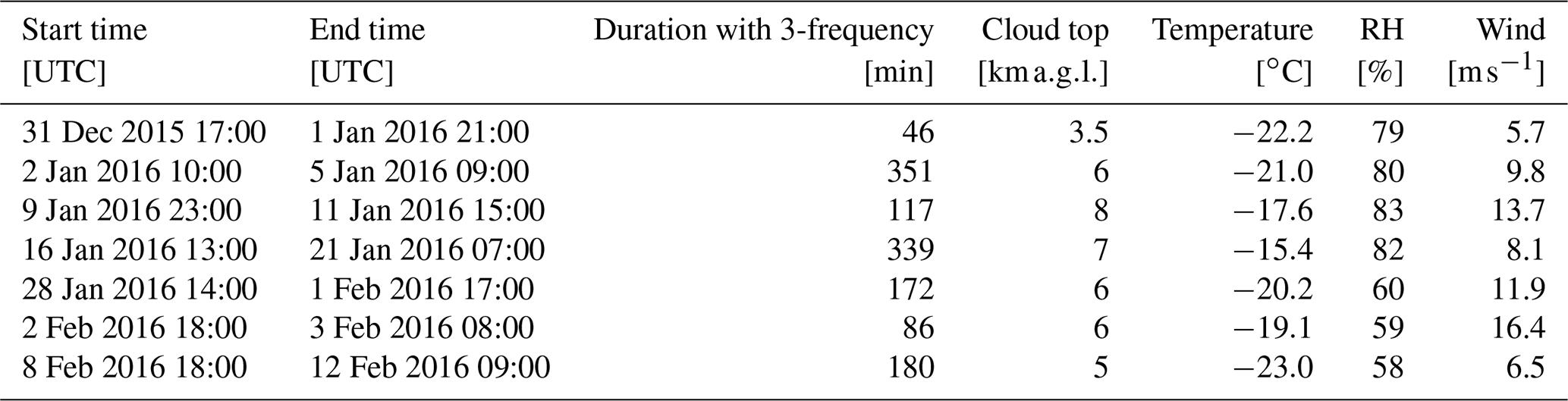
In order to investigate the conditions at which the aggregation and riming processes occur, another way of showing the triple-frequency signatures is to plot the profiles of the observed DWRs after they have been stratified according to air temperature (Fig. 1a, b), as suggested by Dias Neto et al. (2019) for their TRIPEx dataset. To this end, the temperature information was interpolated from the closest radio soundings, which were launched every 12 h during AWARE.
For comparison, the same methodology (Fig. 1c, d) was also applied to the triple-frequency dataset of the BAECC field campaign (Petäjä et al., 2016), during which the ARM program deployed the AMF2 (i.e., the same instruments as for AWARE) at the Hyytiälä Field Station of the University of Helsinki, Finland (61∘50′37.114′′ N, 24∘17′15.709′′ E, 150 m a.s.l.) from 1 February to 12 September 2014. During the winter season, 20 snowfall events were recorded, resulting in 35 h of triple-frequency radar data. Most of the snowfall was associated with deep frontal systems bringing moist air from the Baltic Sea. The most important case studies have already been thoroughly analyzed in previous papers (e.g., Kneifel et al., 2015; Kalesse et al., 2016; von Lerber et al., 2017; Moisseev et al., 2017; Mason et al., 2018, 2019; Tridon et al., 2020). Interestingly, the BAECC DWR density plots are practically identical to those from TRIPEx (Fig. 9 in Dias Neto et al., 2019), with both sites representing well the Northern Hemisphere mid-latitudes.
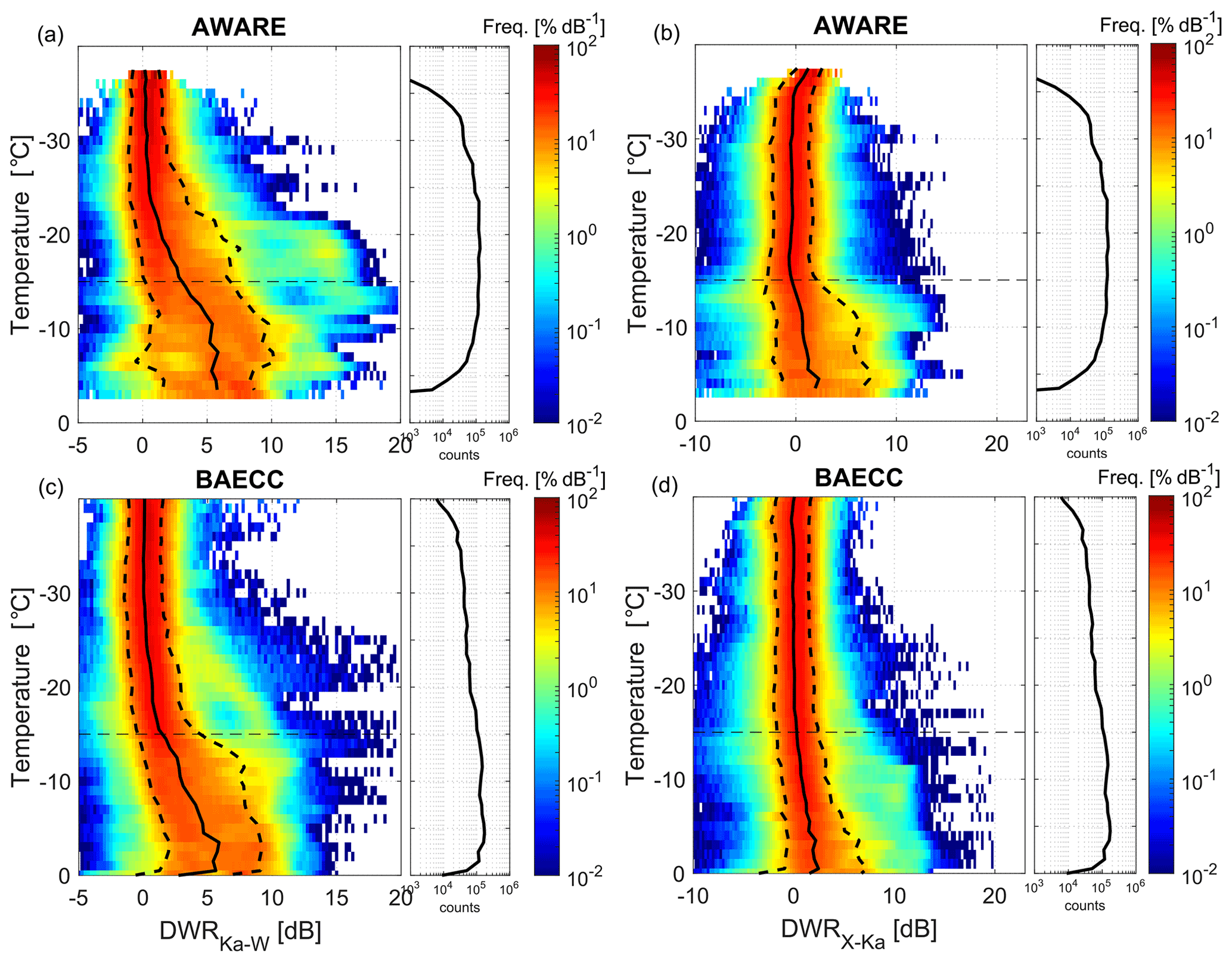
Figure 1Density plots of DWRKa,W (a, c) and DWRX,Ka (b, d) as a function of temperature for AWARE (a, b) and BAECC (c, d) datasets. The dashed lines indicate the 10th and 90th percentiles. The subplots on the right of each panel indicate the number of samples per temperature level.
Despite appearing a bit noisier due to the slightly reduced size of the dataset (i.e., 21 vs. 35 h), the AWARE density plots (Fig. 1) show interesting similarities in comparison with those from BAECC (and, equivalently, TRIPEx), but also some striking differences. In terms of similarities, the medians of both DWRs (black lines) reach nearly the same maxima around 0 ∘C (6 and 2 dB for DWRKa,W and DWRX,Ka, respectively). Furthermore, the rate of increase of the DWRX,Ka with temperature is similar: it remains small at low temperatures and increases faster for temperatures greater than −15 ∘C, which can be explained by a rapid growth of aggregates favored by the dendritic growth around −15 ∘C. Regarding disparities, the AWARE DWRKa,W increases at a lower temperature (around −25 ∘C) compared to the mid-latitude sites. Both the median and the width of the distribution of DWRKa,W increase significantly more for AWARE than for BAECC. Specifically between −25 and −15 ∘C, the median and width increase by 2.6 and 2.4 dB for AWARE, while they only increase by 1.2 and 1.8 dB for BAECC. This is a very peculiar feature that was never observed in the previous yet longer field campaigns during which triple-frequency radar measurements were collected. Furthermore, there is a secondary but striking branch of DWRKa,W reaching extreme values of 15 dB, much higher than the common maximum of 12 dB. Even if it only represents 6 % of the AWARE triple-frequency dataset, this corresponds to 75 min. It was observed during two different cases: the case of 2–4 January 2016, which will be partly discussed in Sect. 4, and case of 9–10 January 2016, which has already been described in Lubin et al. (2020).
If Ka and W band were the only radar pair available, it could be argued that an enhancement of aggregation due to local dynamic effects may be the most probable process leading to the increase of DWRKa,W at low temperature. However, the corresponding DWRX,Ka remains close to 0 dB, which can only be explained by the presence of rimed particles at lower temperatures during AWARE. While we cannot exclude a potential influence from vertical winds induced by the complex topography around McMurdo Station, these differences from previous studies can more likely be explained by the low concentration of aerosol in Antarctica compared to the Northern Hemisphere: a low cloud condensation nuclei concentration could lead to fewer but larger supercooled droplets (for a given cloud water content), and therefore, more efficient riming (Lohmann, 2004). Indeed, even with a smaller number of droplets, the riming process can be favored in a clean environment because the collision efficiency between an ice crystal and a liquid droplet strongly increases when going from small cloud droplets to slightly larger drizzle (Pruppacher and Klett, 2010; Wang and Ji, 2000). In the rest of the paper, the occurrence of riming at low temperatures will be further assessed by focusing on the case of 2–4 January 2016, which features the strongest DWRKa,W of the AWARE dataset.
4.1 General description of the case study
Between 1 and 4 January 2016, the weather conditions were typical of the frequent strong katabatic wind events recorded at McMurdo Station (Chenoli et al., 2013; Coggins et al., 2014; Monaghan et al., 2005; Weber et al., 2016). The Ross Sea semi-permanent cyclonic circulation (Carrasco and Bromwich, 1994; Monaghan et al., 2005; Simmonds et al., 2003) deepened and moved to the south, bringing moist air over the Ross Ice Shelf (see Fig. 2a). MODIS cloud phase retrieval (see Fig. 3) indicates that clouds formed over the ice shelf, including extended clouds with supercooled liquid at their top. The evolution of cloud features in the subsequent panels of Fig. 3 demonstrates the cyclonic (clockwise) circulation centered around the north of the Ross Ice Shelf, which led to deeper ice-topped clouds along the Transantarctic Mountains to the west of the Ross Ice Shelf (see Fig. 2c, d). Cloud initiation mechanisms included lifting of air due to the relief barrier and convergence of cyclone winds with katabatic winds descending from the Antarctic Plateau. Between 2 and 4 January, this resulted in strong southerly winds (e.g., winds up to 16 m s−1 were recorded at 1.7 by the radiosonde launched from the AMF2 at McMurdo on 4 January at 11:00 UTC as shown in Fig. 2b) associated with long-lasting clouds deepening on the windward side of Ross Island.
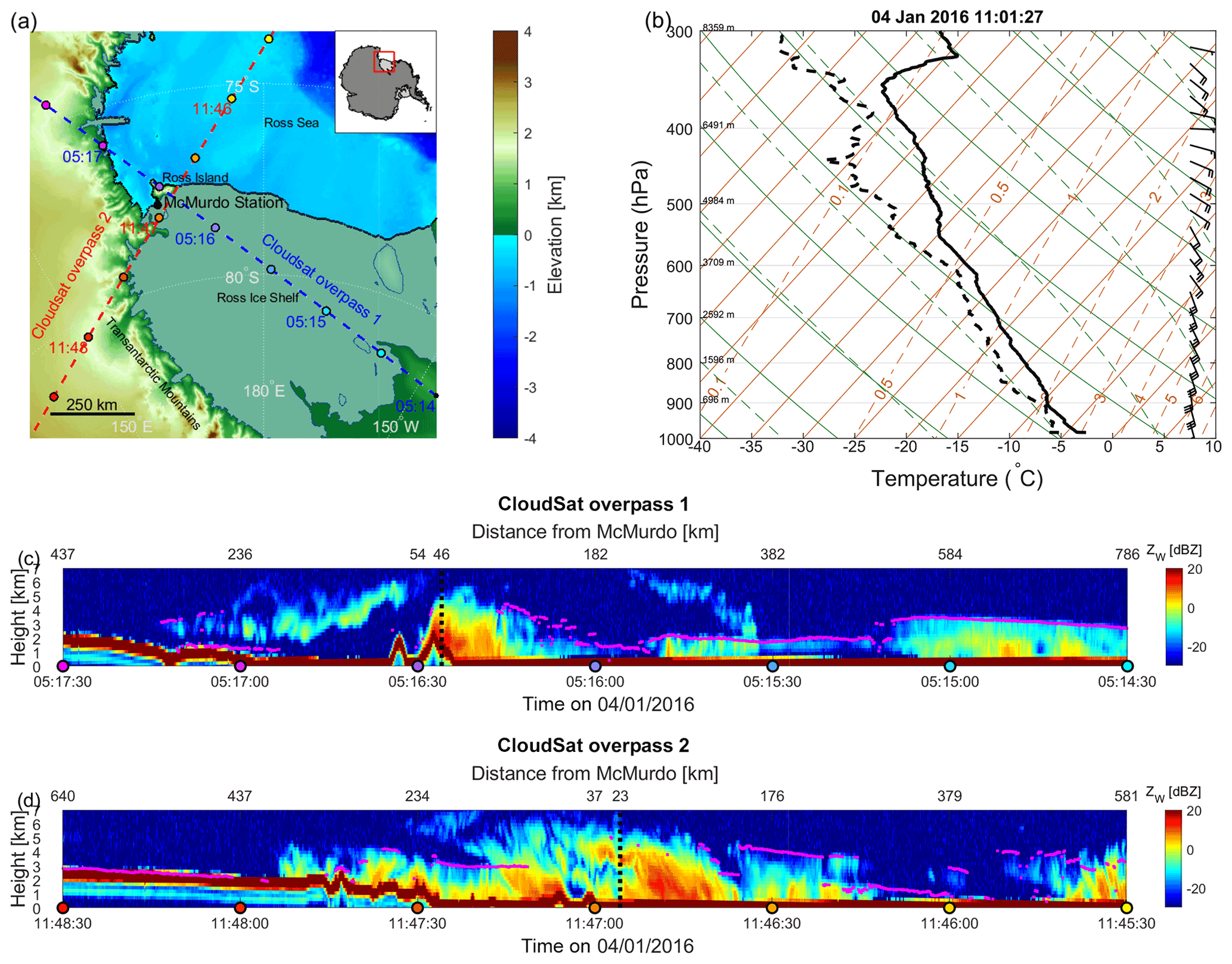
Figure 2(a) Overview of the geographical features around McMurdo created with the Antarctic Mapping Tools for MATLAB (Greene et al., 2017). (b) Profiles of atmospheric temperature (continuous line) and dew point temperature (dashed line) measured by the 10:24 UTC sounding from the AMF2 on 4 January. Time–height cross sections of the reflectivity measured during the ascending (c) and descending (d) CloudSat overpasses closest to McMurdo for the same day, indicated by the dashed blue and red lines in (a) (the colored circles in a and along the x axis of c, d are spaced by 30 s timesteps along the satellite path (equivalent to 228 km) and allow us to visualize the position of the cloud system better). The vertical dotted black lines in (c) and (d) show the time of the closest approach for each overpass, and magenta lines indicate supercooled liquid water clouds as detected by CALIPSO.
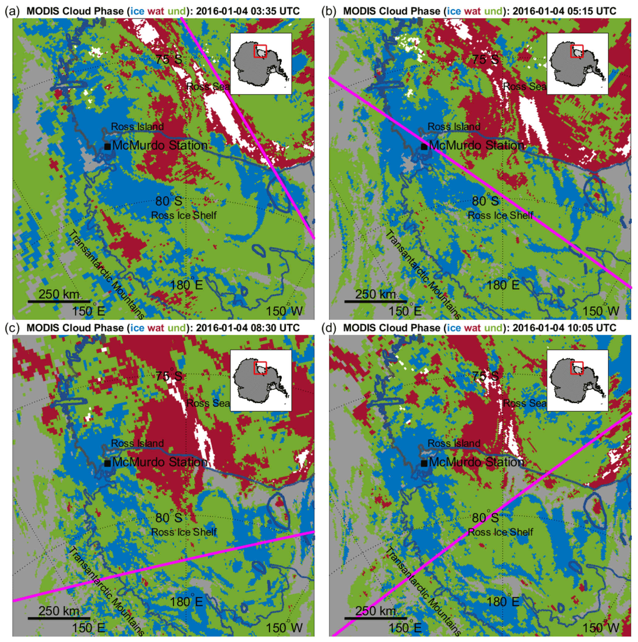
Figure 3Time evolution of cloud top phase (ice, liquid or undetermined in blue, red and green, respectively) retrieved by subsequent MODIS overpasses on 4 January at (a) 03:35, (b) 05:15, (c) 08:30 and (d) 10:05 UTC within the geographical area shown in Fig. 2a. The magenta lines correspond to the satellite ground track for each overpass.
On 4 January 2016, CloudSat made two overpasses exceptionally close to McMurdo Station (as close as 46 and 23 km at 05:16 and 11:47 UTC, respectively). CloudSat reflectivity transects (Fig. 2c and d) confirm the presence of extended and complex cloud fields over the whole Ross Ice Shelf, and particularly deep clouds near McMurdo with cloud tops reaching nearly 6 and reflectivity as large as 14 dBZ. Furthermore, co-located CALIPSO observations indicate that most of these clouds were mixed-phase clouds with a supercooled liquid layer at their tops at temperatures as low as −35 ∘C (magenta lines in Fig. 2c and d).
4.2 Observations at McMurdo
Over McMurdo, a persistent thick cloud layer was continuously observed between 2 and 5 January 2016. While the ARM lidars were not able to penetrate through the full extent of the clouds and sample their top, the associated liquid cloud base height products (Silber et al., 2018b, c) suggest that supercooled liquid layers were almost always present at various heights within the clouds, from 0.5 to 3 for the whole 3 d (not shown).
4.2.1 Unusual dual-wavelength ratios and intense riming
Of particular interest on 4 January is the period between 07:00 and 12:00 UTC, which is associated with a persistent supercooled liquid layer around 2 and characterized by clouds with the largest reflectivities (Fig. 4a). After applying the climatological relative calibrations determined for the whole AWARE field campaign (see Sect. 2.2), effective DWRX,Ka and DWRKa,W are derived (Fig. 4b and c, respectively).
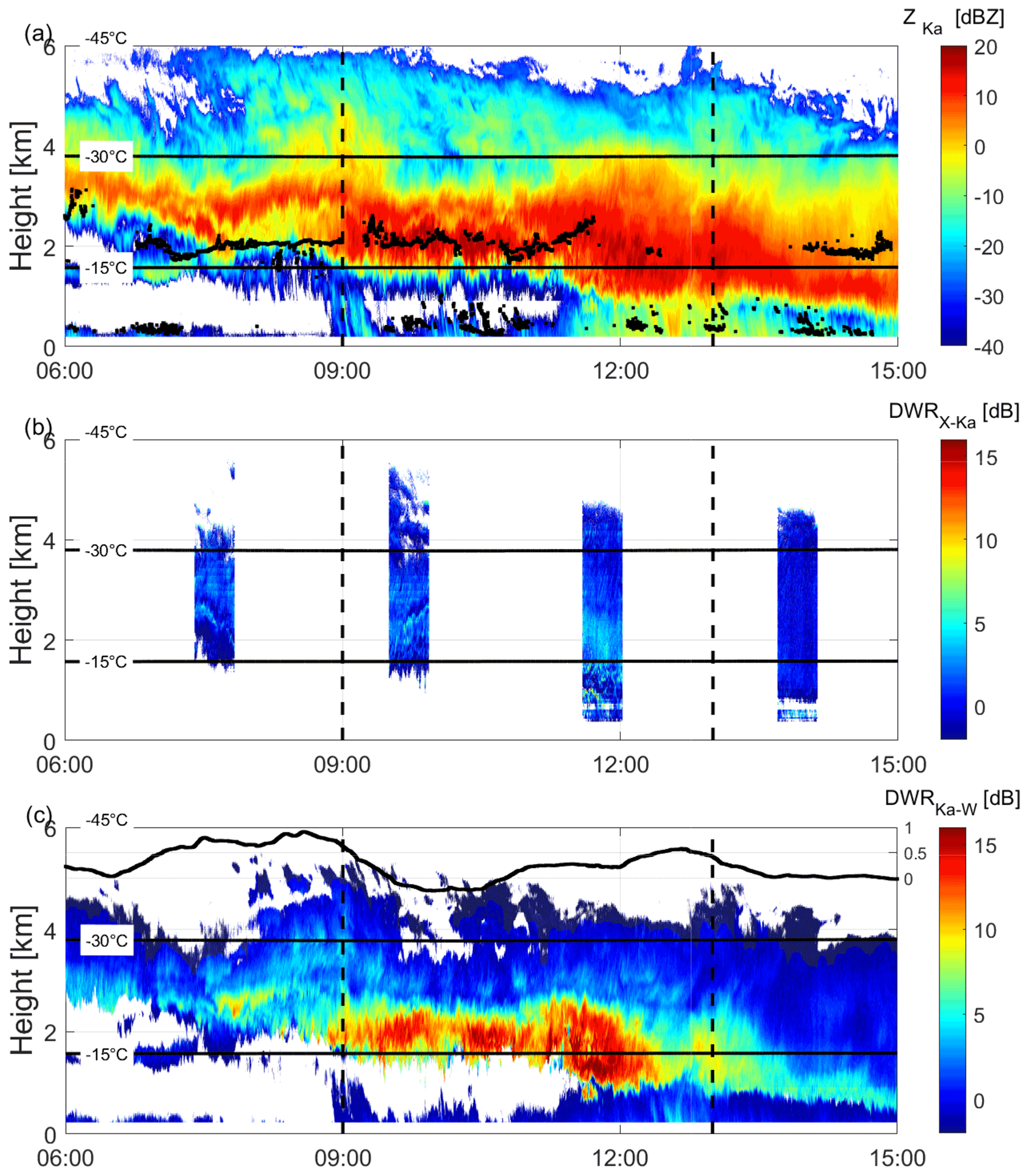
Figure 4Time–height cross section of the (a) KAZR reflectivity, (b) DWRX,Ka, (c) DWRKa,W. The horizontal black lines indicate the −15 and −30 ∘C levels while the vertical dashed lines delimit the period of large DWRKa,W used to produce the density plots in Figs. 7, 8 and 9. The black dots in (a) show the liquid water as detected by the ARM high spectral resolution lidar (HSRL) cloud base height product (Silber et al., 2018b; see also the inset in Fig. 13a). The thick black curve in the upper part of (c) is the two-way ΔPIA in dB (scale along the right axis) derived from Rayleigh scattering hydrometeors at cloud top (gray-shaded zones) following Tridon et al. (2020).
Microwave radiometer measurements were not available at McMurdo before 29 January 2016. Before that date, the liquid water path can still be roughly estimated thanks to multifrequency radar observations (Tridon et al., 2020): using the Rayleigh plateau technique, Rayleigh reflectivity regions at cloud top can be identified (gray-shaded zones in Fig. 4c) and used to derive the two-way differential path-integrated attenuation (ΔPIA, thick black line at the top of Fig. 4c associated with its own scale on the right axis in dB). While ΔPIA can generally be due to thick layers of supercooled liquid droplets or dense snow, the ice crystals in this case study are not expected to produce any significant attenuation. ΔPIA can then be used to roughly estimate the supercooled liquid water path within this cloud (Tridon et al., 2020). Before 07:00 UTC and after 14:00 UTC, ΔPIA is very close to 0 dB suggesting that the ice water path (IWP) and liquid water path (LWP) are small and do not produce any detectable differential attenuation. During the period with the largest DWRKa,W (between 10:00 and 12:00 UTC), ΔPIA reaches 0.25 dB. Assuming that only the supercooled liquid water contributes to the ΔPIA, the corresponding LWP should be of the order of 100 g m−2, according to recent refractive index models (Tridon et al., 2020). Note that ΔPIA becomes slightly negative (−0.25 dB) between 09:30 and 10:30 UTC. This may be linked to the light snow shower reaching the ground around 09:00 UTC, and can be explained by snow accumulating preferentially on the KAZR large flat radome. If this effect persists over the following hours, the true ΔPIA between 10:00 and 12:00 UTC could be at most 0.5 dB, corresponding to an LWP of the order of 200 g m−2.
In the upper part of the cloud (4–6 ) where the temperature is between −25 and −40 ∘C, the reflectivity and DWRs remain low. As aggregation in this temperature regime can be expected to be relatively weak, we expect plate-like particles and possibly polycrystals to dominate. Closer to the supercooled liquid layer, the DWRX,Ka is found only slightly enhanced (up to 5 dB, Fig. 4b) while the DWRKa,W reaches the rather extreme value of 15 dB (Fig. 4c), i.e., the largest values in the AWARE field campaign data depicted in Fig. 1a. At temperatures lower than −15 ∘C, aggregation is still expected to be limited and it is unlikely to be the process which leads to very large DWRKa,W since DWRX,Ka would also be more strongly enhanced if the 15 dB were due to large aggregates. Conversely, such DWR combination strongly suggests an intense riming event, but this assumption cannot be readily corroborated by Doppler velocity because the entire period is affected by significant vertical motions.
4.2.2 Updrafts and mean fall velocity
The KAZR Doppler velocity, (positive when downward in our convention), is the result of the vertical air motion and the ice particle fall speed. For many instances of the case study, it features periods with negative values (Fig. 5a), i.e., updrafts. These updrafts are even more evident when exploiting KAZR Doppler spectra: the Doppler velocity of the slow edge of the spectra (i.e., the vertical velocity of the smallest hydrometeors detected in the sampling volume) is practically always negative (i.e., upward), and in some regions by almost 2 m s−1 (Fig. 5b).
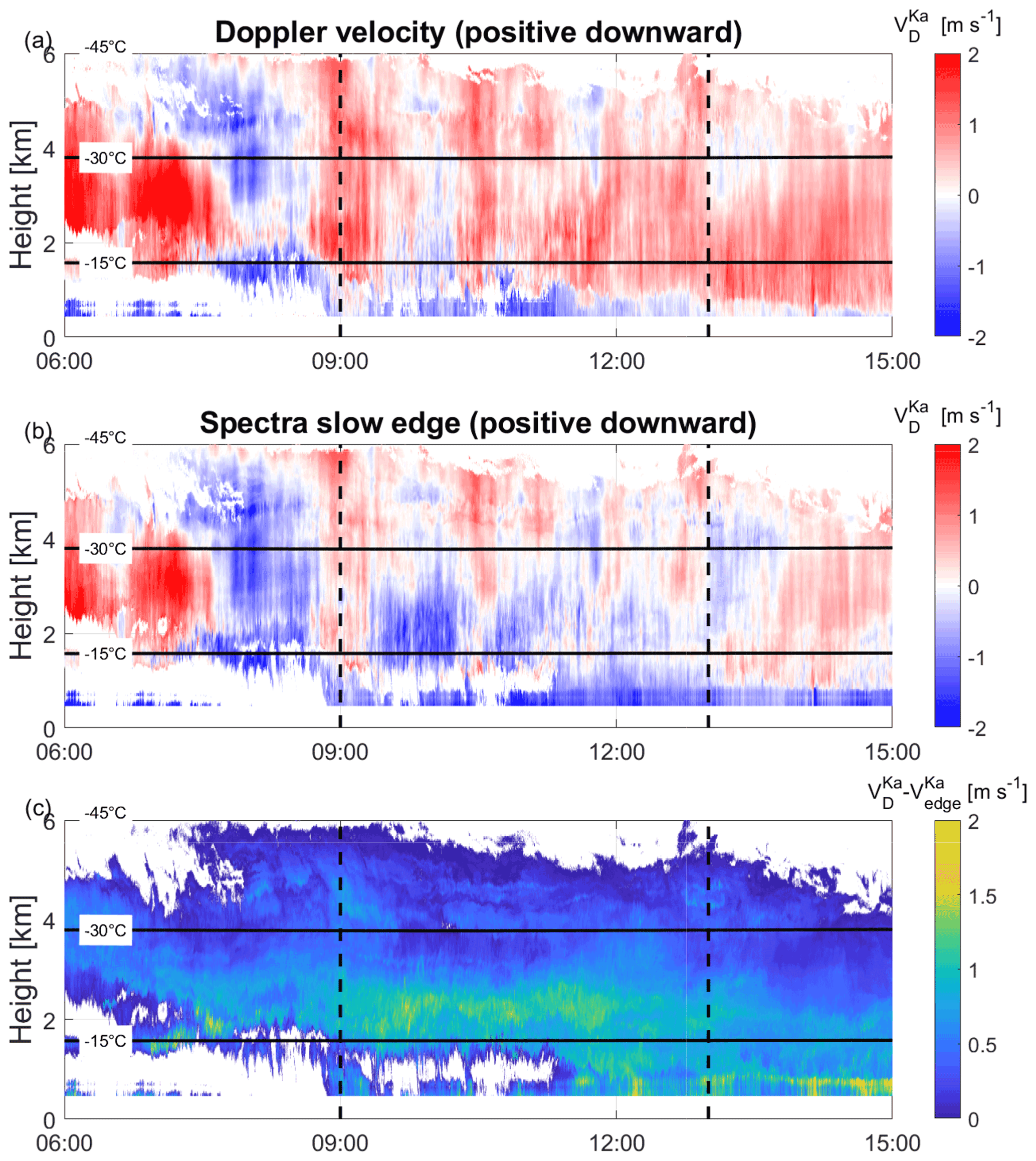
Figure 5Time–height cross section of the (a) KAZR Doppler velocity , (b) Doppler velocity of KAZR spectra slow edge , (c) difference between KAZR Doppler velocity and Doppler spectra slow edge . The horizontal black lines indicate the −15 and −30 ∘C levels while the vertical dashed lines delimit the period of large DWRKa,W used to produce the density plots in Figs. 7, 8 and 9.
During the period analyzed, turbulence broadening is generally low (see Fig. 6a; further discussed in the following section). In such a case, subtracting the slow-edge Doppler velocity from the Doppler velocity gives a reasonable estimate of the reflectivity weighted mean fall velocity, or in other words, the Doppler velocity corrected from vertical air motion (Fig. 5c). This estimate is, however, a lower limit because the smallest hydrometeors detected by the radar may not have a negligible fall speed, an issue which will be exacerbated in regions of low radar sensitivity. In such instances, the actual updraft and, consequently, the derived mean fall velocity would both be underestimated. Nevertheless, such correction must be taken with caution because, in the case of a high level of turbulence, it would lead to a large overestimation of the updraft and of the mean fall velocity.
Figure 5a and b ( and ) clearly show vertical bands that alternate between variable saturation of blue and red colors typically due to alternating updrafts and downdrafts. After subtracting the slow-edge Doppler velocity from the Doppler velocity (Fig. 5c), there is no longer an abrupt change in time and the fall velocity gets larger toward the ground as expected for ice particles growing via deposition, riming or aggregation while they fall through a cloud. This suggests that the contribution of vertical air motions to the Doppler velocity has been correctly eliminated by exploiting the slow edge of Doppler spectra.
The fall velocity of unrimed aggregates is known to be capped at around 1 m s−1, independent of their size because the increase of mass via aggregation is compensated by the enhanced drag due to the larger cross-sectional area (Zawadzki et al., 2001; Kneifel and Moisseev, 2020). With values often reaching 1.4 m s−1 between 1.8 and 3 (Fig. 5c), the resulting mean fall velocity supports the presence of at least slightly rimed ice particles.
4.2.3 Limited turbulence and unusual spectral width signatures
Less directly, the spectral width σD can be used to infer some information on ice properties as well (Maahn and Löhnert, 2017). The challenge is to separate the broadening due to the spread of hydrometeor fall velocities from the broadening due to air motion. For a vertically pointing cloud radar, the air motion broadening is mainly due to turbulence, wind shear and cross wind within the scattering volume (Borque et al., 2016). During this case study, the spectrum width observed by the KAZR (Fig. 6a) is mostly limited to rather small values compatible with the narrow spread of ice crystal fall velocity while only few layers with larger values are probably associated with gravity waves. Since the sampling volumes of KAZR and MWACR are very similar (due to the same range resolution and similar beam widths, i.e., 0.33 and 0.36∘, respectively), air motion broadening should be identical for both radars. Any difference must be related to differential non-Rayleigh effects associated with large ice crystals when they are present, e.g., resulting in a narrower Doppler spectrum at the higher radar frequency. Interestingly, the MWACR spectral width is significantly larger than the KAZR spectral width in the large DWRKa,W region (Fig. 6b), which leads to a negative differential spectral width between Ka and W bands (Fig. 6c). While the spectral width is expected to be larger at Ka bands in general, such a peculiar behavior is possible for narrow size distributions of large ice crystals, as will be seen in Sect. 4.4.

Figure 6Time–height cross section of the (a) KAZR spectral width , (b) MWACR spectral width and (c) differential spectral width between KAZR and MWCAR . The horizontal black lines indicate the −15 and −30 ∘C levels while the vertical dashed lines delimit the period of large DWRKa,W used to produce the density plots in Figs. 7, 8 and 9.

Figure 7Contoured frequency by altitude diagram of the differential fall velocity and differential spectral width between KAZR and MWACR during the period of high DWRKa,W in between the vertical dashed lines in Fig. 4c. The continuous and dashed black lines show the profiles of the median, 10th and 90th percentiles of the distributions.
In order to verify that the negative is not a spurious signal due to a possible mismatch of the radar beams, two-dimensional histograms (contoured frequency by altitude diagram, CFAD) of the differential Doppler velocity () and for the period with high DWRKa,W are shown in Fig. 7. Above 3 , reflectivity, DWRs, and fall velocity are small (Figs. 4 and 5) suggesting that mostly small ice particles, thus Rayleigh scatterers, are present. In this case, both and should be very close to 0. When non-Rayleigh targets are present, the Doppler velocity (still with a positive when downward convention) is generally smaller at the higher radar frequency because scattering effects reduce the backscatter cross section of the largest and faster falling ice crystals. The slightly negative (−0.5 m s−1) – and hence larger – can only be explained by one of the radars slightly pointing off-zenith, as was found for the BAECC dataset (Kneifel et al., 2016). As a result, a small component of the horizontal winds is found along the pointing direction of the mispointing radar, which explains the observed difference. Conversely, being defined as the spread around the mean Doppler velocity, the spectral width is not affected by a bias in Doppler velocity. As expected, is centered around 0 for the small ice crystals present above 4 , confirming that the negative below 3 is not an artifact due to mispointing radar beams.
4.3 Qualitative evidence of narrow particle size distributions
The reflectivity observed by the three radars between 09:00 and 13:00 (the period delimited by the dashed lines in Fig. 4) is combined in the so-called triple-frequency space (Fig. 8). The analysis is restricted to heights above 1 km and a signal-to-noise ratio (SNR) larger than −5 dB, resulting in about 130 000 data points (with resolution of 2 s by 30 m). The bullseye cluster centered around 0–0 dB corresponds to the upper part of the cloud (above 4 km) where the ice particles are small and nearly scatter in the Rayleigh regime at all frequencies. The cluster on the right-hand side corresponds to the lower part of the cloud where supercooled liquid water is present. The combination of very high DWRKa,W and rather small DWRX,Ka is known to be the signature of rimed aggregates. In this case, this riming signature appears much stronger than previously observed, with the most frequent points being centered around DWR dB and DWR dB (magenta ellipse) while DWRKa,W rarely exceeded 12 dB in previous triple-frequency radar field campaign datasets (Kneifel et al., 2015; Mason et al., 2018; Dias Neto et al., 2019).
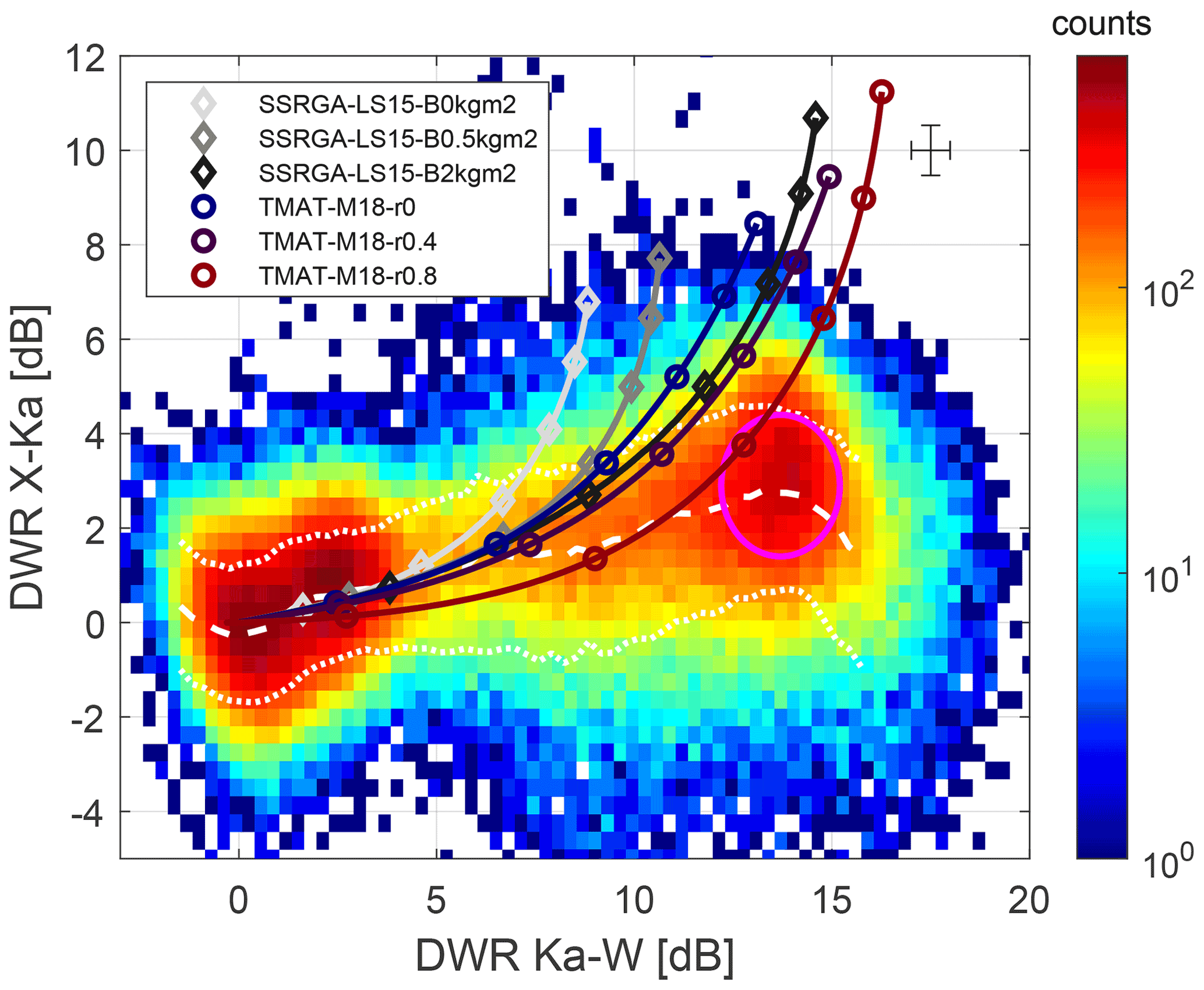
Figure 8Two-dimensional histogram of measured dual-wavelength ratios (DWRs) for triple-frequency radar observations. The superimposed dashed white line shows the median and the superimposed dotted white lines show the 10th and 90th percentiles of the histogram for the DWRKa,W bins containing at least 500 points and the magenta ellipse highlights the unusual triple-frequency signature. The remaining superimposed lines represent the forward-modeled DWR for an exponential distribution of particles with a mean mass diameter comprised between mm (each marker corresponding to 1 mm step) using various electromagnetic-microphysical models (see details in the text). The error bars in the top-right corner represent the intrinsic measurement uncertainties estimated for high SNR according to Doviak and Zrnic (2014).
For reference, the lines superimposed in Fig. 8 show DWRs of exponential distributions of unrimed and rimed ice crystals forward modeled using various state-of-the-art scattering models designated as electromagnetic-microphysical (hereafter EM-MIC) models following the nomenclature introduced in Tridon et al. (2019). A much larger number of scattering models exists but here the focus is on the most realistic ones. For example, models assuming pristine ice crystals with idealized shapes (such as spheres, rosettes or dendrites) are not shown. Light gray to dark gray lines correspond to the self-similar Rayleigh–Gans approximation (Hogan and Westbrook, 2014; Hogan et al., 2017) for realistic ensembles of ice aggregates (B model of Leinonen and Szyrmer, 2015) with various degrees of riming (from unrimed SSRGA-LS15-B0kgm2 to heavily rimed SSRGA-LS15-B2kgm2). Note that the main difference between these SSRGA-LS15-Bxxx models is the quantity of supercooled water accreted to the ice particle, i.e., the degree of riming, but during the generation of the ice aggregates, depositional growth and aggregation are intrinsically included by the explicit simulation of the aggregation of monomers of various sizes. Blue, purple and red lines correspond to T-matrix scattering calculations for oblate spheroid ice crystals with an axial ratio of 0.6 and composed of a homogeneous ice–air mixture (soft spheroid model). The different lines correspond to various densities, which are determined from the density factor r introduced by Mason et al. (2018) (from unrimed TMAT-M18-r0 when r=0 to nearly hail TMAT-M18-r0.8 when r=0.8).
During the 4 h of observations merged in Fig. 8, a variety of microphysics processes are certainly occurring, and due to the complexity of ice particles and ice PSD shapes, there is a large natural variability in the observations. On the contrary, the scattering models can only represent an average behavior of a mixture of ice habits. The objective here is to find the scattering model which best matches the observations on average and, hence, to detect, from the observed reflectivity signatures, the fingerprints of the dominant microphysical process in shaping the ice particles. However, multifrequency radar observations are inevitably noisy not only because of the possible radar volume mismatch, but also because of the intrinsic noisiness of radar measurements which decreases with increasing SNR (Doviak and Zrnic, 2014). For the configuration of the ARM radars during AWARE, DWRX,Ka and DWRKa,W individual observations are associated with an uncertainty of around 0.5 dB at high SNR (as illustrated by the error bars in the top-right corner of Fig. 8). Nevertheless, the median and 10th and 90th percentiles of the density plot as a function of DWRKa,W (white lines in Fig. 8) highlight the average trend and natural variability of the observations, which can then be compared with the theoretical model lines. At low DWRKa,W, all the scattering models shown in Fig. 8 are in agreement with the trend of the observations. But at large DWRKa,W, Fig. 8 clearly shows that, if exponential distributions are assumed, even the scattering models corresponding to rimed particles deviate significantly from the median of the distribution, and hence none of the selected scattering models seems to convincingly explain the observed unusual triple-frequency signatures.
Mason et al. (2019) showed that the shape of the ice particle size distribution (PSD) can also affect the triple-frequency radar signature: reducing the width of a PSD (e.g., by increasing the shape parameter μ of a gamma PSD) has a similar effect to that of increasing the particle density. As a result and since riming has been shown to be correlated with narrow size distributions (Garrett et al., 2015), a narrow PSD could amplify the triple-frequency signature of riming and is the most plausible way to explain the extreme signature observed in this case.
4.4 Constraining ice particle properties from multifrequency radar observations
In order to take into account the effect of the shape of the PSD (see examples in Fig. 12a), we consider gamma distributions of the form
where D is the maximum dimension of ice particles, Λ and μ are the slope and shape parameters, respectively, is the mean mass diameter, bm is the exponent of the mass–size relation associated with the EM-MIC model and f(μ) is a normalization factor following Testud et al. (2001). In comparison with an exponential distribution, a gamma distribution (with μ larger than 0) leads to larger DWRKa,W for any EM-MIC model (Mason et al., 2019, and Fig. 9a). However, it also leads to a reduced spectral width and, as was shown in Sect. 4.2, the observed negative is a very specific feature and is evidence that the PSD is wide enough to contribute to the spectral width. Therefore, combining the triple-frequency radar signature with the observed σDs offers a way to constrain the best EM-MIC model matching the observations (e.g., by comparing the average trend of the density plots of these observations as a function of the DWRKa,W with the theoretical lines provided by the EM-MIC models such as in Fig. 8). Furthermore, even if the estimation of requires a negligible turbulence broadening and a high radar sensitivity, Sect. 4.2 and Fig. 6 suggest that these conditions are reasonably fulfilled for this case study. Then, since the parameter is unaffected by the vertical wind, it is a further parameter that can be used to evaluate EM-MIC models, contrary to the Doppler velocity. To this end, Doppler spectra with a realistic noise level are simulated following the methodology described in Tridon and Battaglia (2015) and vD,slowedge is determined as being the Doppler velocity of the first bin with spectral reflectivity larger than the noise, as for the observed Doppler spectra (see examples of simulated and observed Doppler spectra in Fig. 12b and c).
The resulting density plots of observations are shown in Fig. 9, in which the superimposed theoretical lines correspond to a new EM-MIC model briefly introduced below. By using a similar methodology, Figs. S1 and S2 in the Supplement provide an assessment of how well the two types of rimed aggregates EM-MIC models discussed in the previous section (i.e., SSRGA-LS15-B1kgm2 and TMAT-M18-r0.4) fit the radar observations. Interestingly, despite choosing the most adequate degree of riming, these models appear to be inconsistent with the measurements for the following reasons:
-
For the SSRGA-LS15 type (Fig. S1), a rather high degree of riming (equivalent liquid water path of 1 kg m−2) is required to produce large enough DWRKa,W. This is very surprising because this EM-MIC model corresponds to heavily rimed particles while the small ΔPIA between Ka and W bands (see Sect. 4.2) suggests that the amount of observed supercooled liquid water is relatively small. This leads to excessive simulated fall velocities and spectral widths, with particularly high at small DWRKa,W, resulting in a completely inadequate sloping of this parameter with increasing DWRKa,W.
-
A much better agreement is found for the TMAT-M18 type when using a density factor r=0.4 and shape parameter μ=4 (Fig. S2). Nevertheless, the resulting and are slightly too large. Furthermore, this model appears less physical since it suggests that very high DWRKa,W (larger than 20 dB) could be reached in the case of very narrow size distributions (μ≥16), while the observations suggest a clear cut-off above 15 dB.
Note that the Doppler velocity comparison is not without uncertainty: first, the proposed vertical air motion correction is an approximation; and second, the hydrodynamic theory for ice particles of complex shape is still a topic of active research, with the different hydrodynamic models proposed in the literature (Böhm, 1992; Khvorostyanov and Curry, 2005; Heymsfield and Westbrook, 2010) known to lead to slightly different fall velocities (different line widths in Fig. 9b). Nevertheless, this uncertainty is much smaller than the large overestimation found with the SSRGA-LS15-B1kgm2 model.
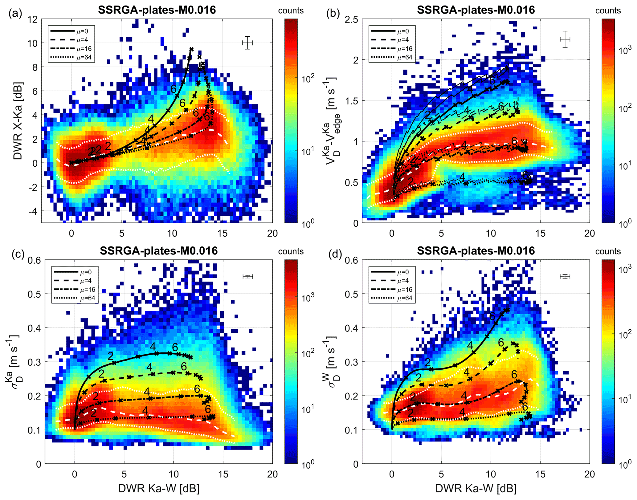
Figure 9Two-dimensional histograms of observed (a) DWRX,Ka, (b) difference between Ka-band Doppler velocity and Doppler spectra slow edge , (c) Ka-band spectral width and (d) W-band spectral width as a function of observed DWRKa,W. The superimposed dashed white line shows the median and the superimposed dotted white lines show the 10th and 90th percentiles of the histogram for the DWRKa,W bins containing at least 500 points. The superimposed black lines represent the corresponding parameters forward modeled with the SSRGA for a gamma distribution of aggregates of plates with various μ (see the legends in the plots), a mean mass diameter of mm (each marker corresponding to 1 mm step) and a normalized rimed mass ℳ=0.016 (see the text for details). The error bars in the top-right corner of each panel represent the intrinsic measurement uncertainties estimated for high SNRs according to Doviak and Zrnic (2014). In (b), thick lines correspond to calculations of fall velocities using the Böhm (1992) model, while thin lines correspond to the Khvorostyanov and Curry (2005) and Heymsfield and Westbrook (2010) models.
A possible explanation for the excessive Doppler velocities of the SSRGA-LS15-B1kgm2 models could be in its mass–size relation. Indeed, the mass–size relation parameters of the Leinonen and Szyrmer (2015) B model for heavily rimed particles are quite different from those derived from various observations according to the comprehensive review made by Mason et al. (2018, their Fig. 1). The rather large prefactor with low exponent leads to particularly large masses for corresponding sizes. While the aggregation and riming model used in Leinonen and Szyrmer (2015) is widely accepted and provides physically reasonable particle shapes (Seifert et al., 2019; Karrer et al., 2020), it remains debatable how realistic it is to cluster the ice particles by the equivalent LWP of supercooled droplets through which they sediment. This model indeed assumes an ideal seeder-feeder cloud situation with the same riming efficiency at all ice particle sizes.
Instead, we propose to cluster rimed particles according to their normalized rime mass, ℳ, defined by Seifert et al. (2019) as the ratio of the particle mass m to the mass mg of a 700 kg m−3 graupel of equivalent size. Such a parameter is better suited to represent successive stages of riming since its definition literally translates the asymptotic increase of m toward mg, and it allowed Seifert et al. (2019) to illustrate the self-similarity of the conversion of aggregates to graupel-like particle. In order to build new EM-MIC models corresponding to specific ℳ values, we used the open code provided by Leinonen and Szyrmer (2015) and produced an ensemble of rimed aggregates with a wide range of ℳ (leading to more diversified degrees of riming than what was proposed in Leinonen and Szyrmer, 2015). Since the DWRs observed during the case study start to increase in the plate-like growth regime, plate aggregates or polycrystals are quite likely and we chose plates as primary ice crystal shape for the simulations. We then used the Snowscatt tool (Ori et al., 2021) to derive the SSRGA parameters for various ℳ classes. While the full discussion of the resulting rime ice particle classes is beyond the scope of this study and will be fully described in a subsequent paper, the resulting ℳ classes provide mass–size parameters which are significantly different from previous studies, but are consistently increasing (not shown) in agreement with riming theory, in particular, with an exponent increasing from 2 (fractal geometry of unrimed aggregates) to 3 (spherical particles, i.e., fully rimed). Especially for corresponding sizes, these mass–size parameters lead to smaller masses and fall velocities than the Leinonen and Szyrmer (2015) B model. With a normalized rimed mass ℳ=0.016 and a μ value on the order of 16, the resulting slightly rimed particle class provides a reasonable agreement with the observed triple-frequency DWRs, spectral widths, and fall velocity, all at the same time (Fig. 9). In this scenario, the high DWRKa,W cluster in Fig. 9a corresponds to mean mass diameter Dm ranging from 5 to 7 mm. The parameters of the SSRGA-plates-ℳ0.016 model are compared with those of previous EM-MIC models in Table 2. Apart from the mass–size parameters, a significant difference resides in the effective aspect ratio (αeff): for the SSRGA-LS15-B1kgm2 model, it is closer to unity suggesting rounded particles and heavy riming, while SSRGA-plates-ℳ0.016 has a value closer to 0.6, the value widely accepted in the literature and more consistent with slight riming.
Table 2Parameters of the main EM-MIC models used in this study: mass–size relation parameters (prefactor am and exponent bm), effective aspect ratio (αeff) and SSRGA parameters (kurtosis parameter κ, power-law prefactor β and exponent γ, and correction factor ζ1) averaged over the 1–10 mm range of sizes. To obtain the parameters of the other EM-MIC models of Fig. 8, the reader can refer to Leinonen and Szyrmer (2015) and Mason et al. (2018) for the SSRGA-LS15 and TMAT-M18 series, respectively.

n/a – not applicable.
4.5 Retrieval of ice properties
In order to constrain the ice particle properties from multifrequency radar observations, numerous assumptions are required. The most important one is the EM-MIC model (and its associated mass–size relation) chosen to describe the type of ice particles. In an effort to evaluate the uncertainty associated with this choice, a simple retrieval of ice properties using the multifrequency radar data and the most likely ice particle types is proposed in this section. The objective here is to find whether an EM-MIC model can describe the triple-frequency radar observations of this case in a physically consistent way. A fully realistic retrieval of the microphysics properties is out of the scope of this study and would require a methodology based on an ice model providing continuous description of ice properties and scattering cross sections as a function of the degree of riming similarly to what was proposed by Leinonen et al. (2018) and Mason et al. (2018).
The retrieval assumes an EM-MIC model and is applied for each ice particle type independently. Its aim is to retrieve parameters such as ice particle number concentration ni, ice water content (IWC) and mean mass diameter Dm. To do so, it is required to invert the ice particle size distribution (PSD). By assuming a gamma PSD (Eq. 1), three parameters must be retrieved: , μ and Dm. It has been shown that the use of a maximum ice particle size Dmax has a significant impact on radar retrievals (Gergely, 2019). Nevertheless, because we want to mainly focus here on the impact of the choice of the EM-MIC model, we decided to fix Dmax to 3 times Dm, following Szyrmer and Zawadzki (2014). The core of the methodology is to retrieve μ and Dm via a simple minimization technique (such as in Turk et al., 2011) and its main steps are as follows:
-
For each EM-MIC candidate, we build a multidimensional lookup table that provides the forward simulated DWR, DWR and at the Ka band (where the Ka subscript is omitted for simplicity) corresponding to any μ−Dm pair.
-
For each combination of measurements, DWR, DWR and , the best matching μ−Dm pair is found by minimizing the cost function CF:
where , and represent the sum of the measurement uncertainties and natural variability of these observations. Based on the joint histograms of Fig. 9, these uncertainties have been set to 3 dB, 1.5 dB and 0.2 m s−1, respectively. This provides a direct mapping from a set of measurements DWR, DWR and to the unknowns μ−Dm.
-
The mapping from the measurements to the unknowns is highly non-linear. The uncertainty associated with this variability is taken into account via Monte Carlo propagation. Namely, the retrieval is performed several times on an ensemble obtained by perturbing each measurement via normally distributed measurement uncertainties with standard deviations , and , respectively. For each set of measurements, a μ−Dm pair is retrieved and the resulting retrieval uncertainties σμ and are obtained by taking the standard deviation of the ensemble of retrieved μ and Dm values.
-
Once μ and Dm and their uncertainties are retrieved for a data voxel, can be directly derived from the observed reflectivity ZKa thanks to the relation
while its standard deviation is computed via error propagation, assuming that σμ and are independent.
-
Finally, IWC and ice number concentration ni and their uncertainties are computed using
where am and bm are the prefactor and exponent of the mass–size relation associated with the EM-MIC model.
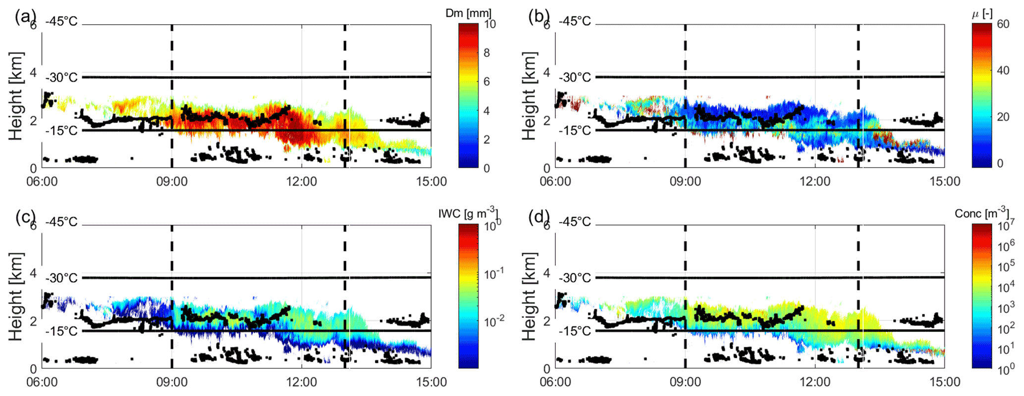
Figure 10Time–height cross section of the retrieved (a) Dm, (b) μ, (c) IWC and (d) Ni when using the SSRGA-plates-ℳ0.016 model, for all pixels where DWRKa,W is larger than 4 dB. The black dots show the location of supercooled liquid water as detected by the ARM high spectral resolution lidar.
The retrieval is applied with the three EM-MIC models, which were found to better describe the joint histograms of observations in Figs. 9, S1 and S2: SSRGA-plates-ℳ0.016, SSRGA-LS15-B1kgm2 and TMAT-M18-r0.4. As an example, Fig. 10 illustrates the results of the retrieval using the SSRGA-plates-ℳ0.016 model. For simplicity, it is applied only to the data identified as rimed by requiring the DWRKa,W to be larger than 4 dB (of course, such a simple threshold is valid for this particular case study only because aggregation is negligible in the unrimed part of the cloud). Apart from μ, which appears slightly noisy, the retrieved fields are reasonably homogeneous, i.e., there is a good spatial coherence. Even though the retrieved μ values may appear anomalously large, the retrieved Λ (not shown) range between 1 and 5 mm−1, consistently with previous studies (Brandes et al., 2007; Gergely, 2019). From 2.6 to 2.3 , Dm strongly increases toward the ground, highlighting the layer where riming is the most efficient and the probable top of the supercooled liquid layer. From 2 downward, there is a clear decrease of ni and IWC, consistent with sublimation of snow when it mixes with dry air in the boundary layer.

Figure 11Comparison of (a) Dm, (b) μ, (c) IWC and (d) ni profiles at 11:58:09 UTC retrieved with the most probable EM-MIC models identified in Sect. 4.4. Colored shadings show the corresponding uncertainties obtained via Monte Carlo propagation as described in the retrieval methodology.
The fields of parameters retrieved with SSRGA-LS15-B1kgm2 and TMAT-M18-r0.4 (not shown) are similarly homogeneous as for SSRGA-plates-ℳ0.016. However, significant and consistent differences are found throughout the entire case study. For simplicity, the retrieved parameters are compared in Fig. 11 for a single profile at 11:58:09 UTC where the DWRKa,W is maximum, but the results are similar for all other profiles. While all three EM-MIC models agree fairly well on the retrieved μ values peaking at 20 between 1.4 and 2.2 , the range of Dm values is not very well constrained owing to the discrepancies between the EM-MIC model attributes (Table 2): SSRGA-plates-ℳ0.016 suggests Dm values about twice as large as SSRGA-LS15-B1kgm2. Sensitivity tests (not shown) indicate that this large difference is mainly due to the unexpectedly high aspect ratio associated with the SSRGA-LS15-B1kgm2 model. With a smaller and more realistic aspect ratio, the particles of the SSRGA-plates-ℳ0.016 model have a shorter dimension along the scattering direction, resulting in less destructive interferences at higher radar frequencies, a weaker reduction of the backscatter cross section of large particles and, hence, smaller DWRs for corresponding sizes. With TMAT-M18-r0.4, this effect is canceled by the distinct method used for the scattering calculations and the resulting Dm values are close to those of SSRGA-LS15-B1kgm2 by coincidence. In a nutshell, the resulting uncertainty on Dm is large because the particle shape is under-constrained. We can only conclude with confidence that the particles are large, with a Dm on the order of 4 mm or larger. Furthermore, knowing that both the SSRGA-plates-ℳ0.016 and SSRGA-LS15-B1kgm2 models have been derived from the same aggregation and riming model, additional work is needed to determine which aspect ratio is the most realistic and to be able to derive Dm with a better accuracy. Interestingly, ni and IWC retrieved with the three different EM-MIC models are in fairly good agreement despite the large difference in Dm, which suggests that these parameters are rather well constrained when combining reflectivity observed at X, Ka and W bands and the estimate. Likewise, Fig. 11c also shows the IWC retrieved using the climatological IWC-ZKa-T relationships of Hogan et al. (2006) and (for midlatitude Protat et al., 2007). They result in IWCs more than 1 order of magnitude larger than the EM-MIC models, suggesting that such simple statistical relations are not suited for specific conditions like the narrow size distributions of this case.
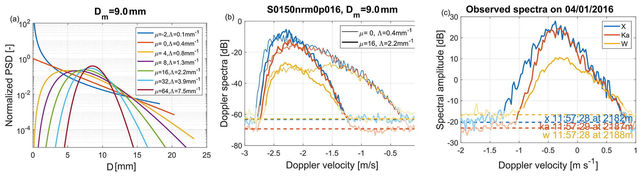
Figure 12(a) Gamma PSDs with Dm of 9 mm and various shape parameters μ (see the legend for numeric values) as a function of the maximum dimension of ice particles. (b) Corresponding Doppler spectra at X, Ka and W band (see color key in c) forward modeled using the SSRGA-plates-ℳ0.016 model, for an exponential PSD (μ=0, thin line) and a narrow PSD (μ=16, thick line). (c) Examples of observed Doppler spectra where similar Dm and μ are suggested by the retrieval using the SSRGA-plates-ℳ0.016 model (see Fig. 11). In (b) and (c), the horizontal dashed lines represent the noise level estimated from each Doppler spectrum and the portions of lines with weak color saturation highlight the parts of the Doppler spectra which are identified as noise.
The three EM-MIC models consistently suggest that the unusual triple-frequency radar signatures were due to narrow PSDs. Even though the retrieved shape parameter values μ=20 are in the high end or above the range commonly found in the literature (Brandes et al., 2007; Tiira et al., 2016; Mason et al., 2019), such PSDs have a sensible shape (Fig. 12a, green line) and the corresponding forward-modeled Doppler spectra (Fig. 12b, thick lines) are comparable to the observed ones (Fig. 12c). When an exponential PSD is used, the forward-modeled Doppler spectra are considerably wider than in the observations, leading to spectral widths much larger than those predominantly observed (see Fig. 9c and d). In order to obtain Doppler spectra as narrow as those observed, with an exponential PSD and the SSRGA-plates-ℳ0.016 model (or the TMAT-M18-r0.4 model, see Fig. S2), a Dm smaller than 1 mm is required, which is then not compatible with the large DWRs observed. This further confirms that narrow PSDs are required to explain the observed triple-frequency signatures.
In summary, despite the lack of in situ observations for constraining the ice particle properties, the detailed exploitation of triple-frequency radar observations allowed us to conclude that the specific radar signature observed during this case study was due to narrow distributions of large and slightly rimed plate polycrystals. It the next section, we devise a bin model experiment to better understand whether riming and such a narrow PSD can be physically consistent.
4.6 Bin model experiment: can a plausible scenario reproduce the observed narrow PSD of rimed ice particles?
In situ airborne observations of ice PSDs over Antarctica are relatively scarce and are commonly performed using instruments such as the Cloud Particle Imager (CPI, Lawson et al., 2001) and the Cloud Imaging Probe (CIP, Lachlan-Cope et al., 2016), which are limited to a particle maximum dimension of ∼1.5 mm. This lack of a comprehensive observational database of Antarctic ice precipitation PSDs combined with instrument-detectable particle size limitations inhibits any pertinent comparison with the results presented here of ice particles with sizes on the order of a few to several millimeters generating the observed triple-frequency radar signatures. Moreover, the elevated altitude range characteristic of these radar signatures further impedes comparisons to ice particle properties derived from Antarctic ground-based observations, which are strongly influenced by low-level ice sublimation (e.g., Grazioli et al., 2017b) and blowing snow events (e.g., Loeb and Kennedy, 2021), frequently occurring over the region. Instead, we performed a modeling exercise in order to establish whether a plausible riming scenario based on AWARE observations could develop the detected triple-frequency signature, thereby adding a physical context to this analysis, which exemplifies that such narrow ice PSDs are realistic.
4.6.1 Model setup and initialization
To examine whether a plausible riming scenario could develop the triple-frequency signature detected in the observations, we use the Distributed Hydrodynamic Aerosol and Radiative Modeling Application (DHARMA) model (Stevens et al., 2002) coupled with the Community Aerosol-Radiation-Microphysics Application (CARMA) size-resolved bin microphysics model (Ackerman et al., 1995; Jensen et al., 1998). Our main hypothesis in this modeling exercise is that the high μ values suggested by the observations are most likely to occur if the ice hydrometeors dominating the radar echoes originate from a shallow generating layer and experience little to no mixing before the combined DWRX,Ka and DWRKa,W signatures are produced. That is because a deep generating layer or strong mixing of rimed ice hydrometeors would necessarily lead to stronger dispersion of size-dependent ice particle fall velocities at given air volumes and broadening of the ice PSD (lower μ). Such broadening of the PSD implies a larger contribution of particle sizes producing lower DWRKa,W and/or higher DWRX,Ka (Fig. 9) to the total output signatures resulting in a deviation from the observed DWR values. This hypothesis is supported by the small spectral width values (Fig. 6a) and the largely stable atmospheric profile during the event indicated by the potential temperature sounding measurements (Fig. 13a).
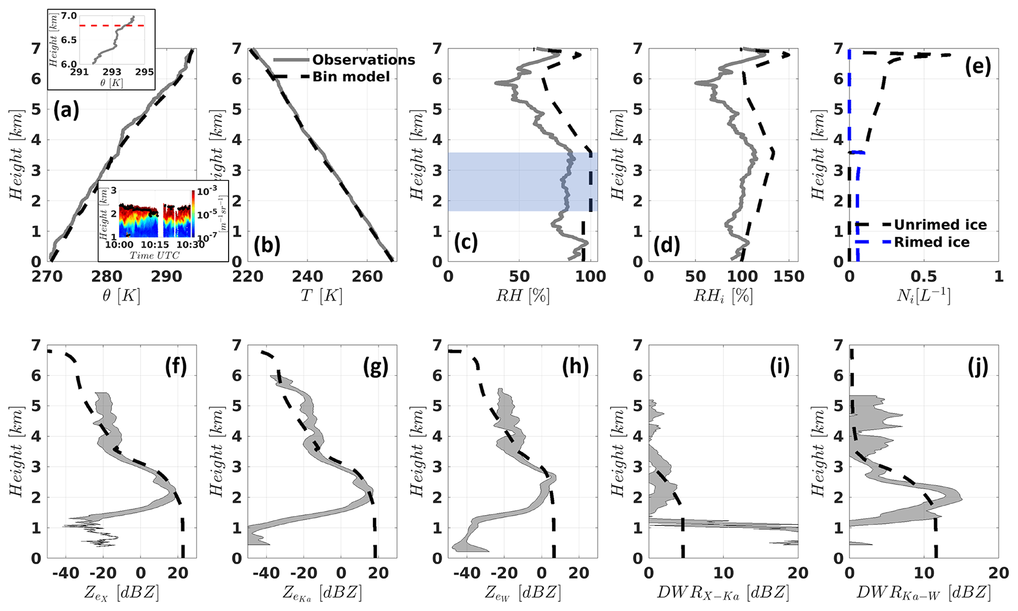
Figure 13Sounding (10:24 UTC) and radar (09:30–09:55 UTC) measurement profiles together with the bin model output at the end of the 8 h simulation. (a) Potential temperature (θ), (b) temperature, (c) relative humidity (RH), (d) RH with respect to ice (RHi), (e) unrimed and rimed ice number concentration (model only; see legend), (f) measured temporal mean ± 1 standard deviation XSACR (shaded region) plus model forward-calculated X-band (dashed black line) reflectivities, (g) as in (f) but for KAZR (Ka band), (h) as in (f) but for MWACR (W band), (i) as in (f) but showing the DWRX,Ka, and (j) as in (f) but showing the DWRKa,W. The blue-shaded rectangle in (c) represents the estimated supercooled cloud extent (see text). The insets in panel (a) depict the θ profile between 6 and 7 altitude with the dashed red line designating the RH peak (see c) at ∼6.8 (top), and backscatter cross section measured with the HSRL around radiosonde release time together with liquid cloud base heights (black markers; see Silber et al., 2018b, c).
As indicated by the cloud base height product (Silber et al., 2018b) applied on the high spectral resolution lidar (HSRL; Eloranta, 2005) measurements (black dots in Figs. 4a and 13a's inset), a distinct supercooled cloud layer was continuously observed over McMurdo Station at altitudes of 1.7–2.5 Nevertheless, the sounding relative humidity (RH) measurements (Fig. 13c) show too low values at these altitudes peaking at 84 %. Considering the cloud field extent during the event based on the satellite measurements (Figs. 2 and 3), we postulate that even with the radiosonde horizontal drift of a few kilometers away from McMurdo until it reached an altitude of 2.5 , it could not reach a cloud-free layer. Therefore, we deduce that the radiosonde RH measurements became negatively biased at some point of the balloon flight by up to ∼ 16 %. We note that such negative RH measurement biases were detected in some other cases during AWARE based on HSRL, KAZR, and sounding cross-validation (not shown), and were occasionally occurring at other sites as well. Based on this deduction and supported by indications of a geometrically thick liquid water layer suggested by a consistent hydrometeor population observed in the KAZR spectra (not shown), we conclude that a deep supercooled layer was extending from about 1.7 to 3.6 , with a possible break of a few hundred meters centering at ∼ 2.6 (Fig. 13c). The location of this deep supercooled layer suggests that even if some vertical mixing did occur during this event (at 3.5–4.2 and 6.4–6.7 ; see vertical potential temperature profiles in Fig. 13a), it mostly took place at altitudes where the ice particle population did not yet experience rapid mass growth due to ice supersaturation conditions (Fig. 13d) and/or intense riming, thereby hindering PSD broadening. The potentially mixed layer between the surface and 1.2 was below the DWR signatures around 2 examined in this study and, hence, had no impact on the observed signatures.
The sounding RH bias also indicates that it is plausible that the ∼ 100 m thick RH peak value aloft of 77.5 % at 6.7 was actually greater, on the order of 93 %–94 %. The source of this elevated shallow high-RH layer could be associated with the apparently mixed ∼ 300 m deep underlying layer potentially transporting relatively warmer and moister air aloft (Fig. 13a and its inset). However, a detailed investigation of this moisture source as well as the generating mechanism of the elevated mixed layer, which could be related to gravity wave breaking, for instance (e.g., Lane and Sharman, 2006; Podglajen et al., 2017), is beyond the scope of this study.
The inferred RH peak values (>90 %) in this elevated layer suggest that homogeneous freezing of humidified aerosols (hereafter aerosol freezing; e.g., Jensen and Ackerman, 2006; Jensen et al., 2001) might have played a role in the initial formation of at least some of the ice population examined in this study, owing to the large RHi values (Fig. 13d), which occurred close to water saturation at a low temperature of −50 ∘C measured at the RH peak altitude (Fig. 13b). Continuous precipitation of ice from an altitude of ∼ 7 is indicated by spaceborne radar echoes over the region (Fig. 2) as well as by the ground-based radar echoes (below ∼ 6 ; Fig. 4). The difference between the topmost radar echoes in the ground-based versus spaceborne measurements could be the result of relatively small ice particles between 6 and 7 (especially if indeed formed via aerosol freezing) combined with the limited ground-based radar detectability at the upper troposphere (e.g., Silber et al., 2021).
Following this discussion while acknowledging that our constraining observations over the depth of the atmospheric profiles are relatively limited in space and time, we use a simplified approach, where possible, to initialize and run the bin model. Thus, we run the model over a one-dimensional (column) domain justified by generally stable atmosphere. We also nudge the bin model simulation thermodynamically (liquid potential temperature and total water) to the local sounding measurements over McMurdo Station (Figs. 2 and 13) using a nudging time scale of 15 min. That is, because the long duration of the triple-frequency signature (∼ 5 h) suggests steady-state Eulerian conditions. Moreover, the highly complex flow fields typical to the McMurdo region (e.g., Silber et al., 2019a; Fig. S1) often result in large reanalysis and regional model biases in reproducing local flow patterns and thermodynamic fields (see Silber et al., 2019c), inhibiting the option of faithfully informing the Eulerian column model with advective tendencies. With the implemented 15 min nudging time scale, our 8 h long sensitivity test simulations typically reach steady state after 3–5 h, allowing us to process and examine the bin model output profiles at the end of the simulation.
Our simplified approach is also incorporated in our treatment of the initialized (and nudged) thermodynamic profile as well as in the treatment of ice nucleation. Ice nucleation is represented only via homogeneous freezing of humidified ammonium bisulfate aerosol or activated droplets (heterogeneous ice nucleation is neglected). Since only aerosol freezing occurs here, the ice number concentrations are effectively determined by the RH maximum within the most elevated moisture layer. In the simulation discussed below, which provided rough agreement with observations, the model is being nudged to an RH peak value of 94 %, consistent with the RH bias discussion above. We note that results similar to the examined simulation at the bottom 3.5 were also obtained in different model simulations (not shown) in which ice nucleation via heterogeneous immersion freezing was included and presented the only source of ice crystals (without aerosol homogeneous freezing aloft, thus omitting the mid-to-upper tropospheric ice); in that case, ice nucleation was concentrated at ∼ 3.6 , at the top of the deep supercooled layer.
The RH profile below the moisture layer peak is set such that the full profile is supersaturated with respect to ice (Fig. 13d), thereby excluding potential ice sublimation and growth convolution effects on the model output. The RH profile is set to be supersaturated between ∼ 1.7–3.6 (Fig. 13c), enabling the formation and persistence of the deep supercooled layer in steady-state. The sounding temperature measurement profile is kept unmodified (Fig. 13). Aerosols are set to a log-normal PSD with a mean diameter of 0.076 µm, a geometric standard deviation of 1.5, and total concentration of 430 cm−3, the values of which are based on monthly mean surface measurement at AWARE for January 2016 (Liu et al., 2018).
The bin model is initialized with a single liquid water group and two ice groups: one for unrimed (pristine) ice and another for rimed ice. Each hydrometeor group consists of 60 bins with a minimum radius of 1 µm and mass ratio between consecutive bin radii of 1.5, allowing for a maximum particle diameter of a few centimeters. For the unrimed ice group, we use mass–diameter and area–diameter power-law parametrizations for radiating plates taken from Fridlind et al. (2012, Table 1), which generally correspond with the polycrystal ice habit regimes (Bailey and Hallett, 2009) of the generating layer, whether it was actually the elevated moisture layer at ∼ 6.7 or at the top of the deep supercooled layer at ∼ 3.6 (Fig. 13). The rimed ice mass–diameter and area–diameter power-law parametrizations we use are the SSRGA-derived parameters for ℳ=0.016 discussed in Sect. 4.4. Collision and accretion between droplets (creating larger droplets or drops), between unrimed ice and droplets (converting to rimed ice), and between rimed ice and droplets (increasing rimed ice mass) are computed from pairwise particle properties (masses, maximum dimensions, aspect ratio, and projected areas) following Böhm (1999, 2004). Aggregation of ice particles is neglected. Consistently, the forward radar calculations are performed using the same SSRGA method informed by the bin model output.
4.6.2 Model results
The model simulation reached steady-state conditions after ∼ 5 h. During steady-state, in-cloud mean droplet number concentration is ∼ 30 cm−3. The domain's LWP is ∼ 220 g m−2, in general agreement with rough LWP estimates on the order of 100–200 g m−2 using the method developed by Tridon et al. (2020). IWP retrievals following Hogan et al. (2006) using the sounding temperature and KAZR reflectivity measurements suggest values during the event on the order of 400 g m−2 (see Fig. 11), the highest IWPs observed during AWARE. The model steady-state IWP values of ∼ 165 g m−2 are in general agreement with these retrievals considering the high uncertainty associated with these (and other) radar-based ice water content retrievals (e.g., Heymsfield et al., 2008).
Figure 13 illustrates profiles of ice particle concentrations (panel e) together with forward-calculated reflectivities and DWRs (panels f–j) corresponding to the end of simulation (8 h). Initial ice nucleation occurs at the elevated RH layer via aerosol freezing with a maximum ice number concentration of ∼ 0.7 L−1 (Fig. 13e). The ice number concentration apparently decreases with height because the ice particle fall velocities increase with decreasing height as their mass becomes larger due to vapor growth under the ice-supersaturated conditions, reaching roughly uniform concentrations with height that are consistently smaller than retrieved, as further discussed below. As the precipitating ice particles reach an altitude of ∼ 3.6 , the ice particles become rimed and quickly gain additional mass.
Intensification of the Ka- and X-band reflectivities at these lower altitudes (from 3.5 to 2.1 ) in which the deep supercooled layer exists (Fig. 13f–g; the W-band reflectivity intensification in Fig. 13h is less pronounced) is commensurate with this rapid mass growth. These reflectivity strengthening patterns and values down to the reflectivity peak (between 2.1–3.5 ) are in reasonable agreement with the radar observations. Note that reflectivity aloft is underestimated in this model simulation by up to several dB, which could be attributable to possible biases in the representation of unrimed polycrystals or underestimated ice number concentrations.
The model-based DWRs within the deep supercooled layer where the triple-frequency signature was detected show key similarities with the observations; that is, the DWRX,Ka is kept at low values (<5 dB) while the DWRKa,W increases to large values of ∼ 12 dB (Fig. 13i–j). These similarities are also evident from Fig. 14a, which shows the spread in the observed DWR values at different height ranges together with the temporally averaged values and the bin model output.

Figure 14(a) DWR parameter space scatter plot showing the observations (09:30–09:55 UTC) at different height ranges, the temporal mean observations (color scale denotes height), and the bin model output at the end of the simulation (8 h) (see legend). (b) Shape parameter (μ) derived from gamma distribution fits for the rimed ice group at different heights. μ values are only shown for fits in which the adjusted r2 is larger than 0.98. (c) Mode and mean diameter of the rimed ice group using the gamma fit parameters under the same adjusted r2 threshold.
To examine the correspondence of this case study's observational analysis conclusions concerning the shape of the ice PSD able to generate the observed triple-frequency signatures (Sect. 4), we perform a gamma distribution fitting to the bin array profile of the rimed ice group at the end of the simulation. Figure 14b shows a profile of μ derived from gamma distribution fits that agree reasonably well with the rimed ice PSD (adjusted r2>0.98). The μ profile indicates a very narrow PSD (μ>40) at the top of the supercooled layer followed by stabilization of μ values at a range of 9–11 at lower heights, which is consistently lower than the best fit to observations (μ∼20). The mean and median ice particle diameters range between 3 and 4 mm over the height range around 2 corresponding to the DWR signatures (Fig. 14c).
Taken together, these model results offer general support for the observational and theoretical analysis of the triple-frequency signatures detected during this event on 4 January 2016 (Fig. 9). Although simulated number concentrations are lower than retrieved and the PSD shapes not as narrow, the overall development of DWR trends with height is generated by the model's standard physics schemes without requiring any special tuning. If model number concentrations are doubled prior to the forward calculations, reflectivity is overestimated relative to the observations (not shown). We have therefore not tried to exactly match retrieved number concentrations and ice PSD widths, also owing to weak constraints on ice crystal properties.
In summary, the bin model simulation corroborates the plausibility of scenarios capable of producing the unique signatures observed during this event. DWR parameter space agreement with the observations could be reached in other sensitivity tests where some vertical motion was introduced or in cases where the nudged sounding profile was slightly modified. However, reaching these high (low) DWRKa,W (DWRX,Ka) values always required some compromises concerning the reflectivity aloft, for example (as in this depicted simulation), thus emphasizing the difficulty to constrain ice properties with our limited observational dataset. Yet, the fact that similar results could be reached using somewhat varying configurations as long they allowed for narrow rimed ice PSD with diameters on the order of a few millimeters to be produced and developed suggests that such cases might occasionally occur over the Antarctic (or other polar regions). The frequency of occurrence of such scenarios will be examined in future studies.
In this work, by exploiting the deployment of an unprecedented number of multiwavelength remote sensing systems (including triple-frequency radar measurements) at McMurdo Station, Antarctica, during the Atmospheric Radiation Measurements West Antarctic Radiation Experiment (AWARE) field campaign, we find frequent occurrences of high Ka–W DWRs coinciding with relatively low X–Ka dual-wavelength ratios taking place at unexpectedly low temperatures of −20 ∘C, in comparison with the mid-latitudes. These features, generally interpreted as riming signatures, suggest a likely common atmospheric state over Antarctica that includes a rather stable atmosphere inhibiting turbulent mixing, and a high riming efficiency driven by large cloud droplets. We note, however, that the limited duration of the triple-frequency dataset collected during AWARE does not allow us to draw definite conclusions concerning the frequency of such events.
A peculiar case study is analyzed in greater detail: it features a persistent layer with relatively modest amounts of supercooled liquid water producing particularly strong riming signatures in triple-frequency radar data. Since in situ observations are lacking, the radar observations are exploited to retrieve the properties of the ice particles leading to these signatures. To this end, several state-of-the-art microphysics and scattering models (EM-MIC models) are used. The combination of the triple-frequency radar reflectivities, the differential spectral width and a proxy of the ice particle fall velocities derived from the Doppler spectra allows us to constrain the microphysical properties of the ice particles. Results suggest that the fall velocity associated with recent rimed aggregate EM-MIC models is too large, and a novel potentially more realistic EM-MIC model is therefore proposed. Even if a non-negligible uncertainty remains on the size of the retrieved ice particles, results indicate that the observed DWR signatures can only be explained by the combined effects of moderately rimed aggregates or similarly shaped florid polycrystals and a narrow PSD. More studies are needed to validate the retrieval algorithm proposed here. This could be done either by cross-comparing the algorithm results with other techniques and/or by using in situ validation datasets from field campaigns (Leinonen et al., 2018; Mason et al., 2018; Battaglia et al., 2020b; Mroz et al., 2021; Nguyen et al., 2022), while noting that commonly used airborne imagers are limited to particles sizes smaller than those deduced in this study.
Simulations of this case study performed with a one-dimensional bin model confirm that, with the modest amount of supercooled liquid water, the triple-frequency radar observations can be generally reproduced, provided that narrow PSDs are simulated. Such narrow PSDs could be explained by two key factors: (i) the presence of a shallow homogeneous droplet or humidified aerosol freezing layer aloft seeding a supercooled liquid layer, and (ii) the absence of turbulent mixing throughout a stable polar atmosphere that sustains narrow PSDs, as hydrometeors grow from the nucleation region aloft to ice particles of several millimeters in size, by vapor deposition and then riming.
This study illustrates that triple-frequency radar measurements can be used to infer detailed properties of precipitating ice such as the PSD width or the degree of riming of ice particles. While the associated retrieval techniques are still at an exploratory stage, such information is crucial for improving our understanding of the role of the ice phase in the water budget. Therefore, more observations and analysis involving triple-frequency radars are needed in the future.
AWARE data were obtained from the U.S. DOE ARM Climate Research Facility https://www.archive.arm.gov (last access: 5 December 2019):
-
Ka ARM Zenith Radar, https://doi.org/10.5439/1095601, Atmospheric Radiation Measurement (ARM) user facility, 2014;
-
Marine W-Band (95 GHz) ARM Cloud Radar, https://doi.org/10.5439/1150242, Atmospheric Radiation Measurement (ARM) user facility, 2015a;
-
X-Band Scanning ARM Cloud Radar, https://doi.org/10.5439/1150303, Atmospheric Radiation Measurement (ARM) user facility, 2015c;
-
Balloon-Borne Sounding System, https://doi.org/10.5439/1595321, Atmospheric Radiation Measurement (ARM) user facility, 2015b.
The supplement related to this article is available online at: https://doi.org/10.5194/acp-22-12467-2022-supplement.
ARM radar data analysis was done by FT and PK. Bin model simulations and their analysis were carried out by IS and AF. Interpretation and writing were shared between FT, IS, AB, SK and AF. RD provided the satellite data.
The contact author has declared that none of the authors has any competing interests.
Publisher’s note: Copernicus Publications remains neutral with regard to jurisdictional claims in published maps and institutional affiliations.
We thank the two anonymous reviewers for their detailed and thorough comments which helped greatly to improve the manuscript.
This work was funded by the US Atmospheric System Research (grant no. DESC0017967). Contributions by Stefan Kneifel were funded by the German Research Foundation (DFG) under grant KN 1112/2‐1 as part of the Emmy‐Noether Group “Optimal combination of Polarimetric and Triple Frequency radar techniques for Improving Microphysical process understanding of cold clouds” (OPTIMIce).
This paper was edited by Timothy Garrett and reviewed by two anonymous referees.
Ackerman, A. S., Hobbs, P. V., and Toon, O. B.: A Model for Particle Microphysics, Turbulent Mixing, and Radiative Transfer in the Stratocumulus-Topped Marine Boundary Layer and Comparisons with Measurements, J. Atmos. Sci., 52, 1204–1236, https://doi.org/10.1175/1520-0469(1995)052<1204:AMFPMT>2.0.CO;2, 1995. a
Atmospheric Radiation Measurement (ARM) user facility (Lindenmaier, I., Bharadwaj, N., Johnson, K., Nelson, D., Isom, B., Hardin, J., Matthews, A., Wendler, T., and Castro, V.): Ka ARM Zenith Radar (KAZRMD), 2015-11-17 to 2017-01-02, ARM Mobile Facility (AWR) McMurdo Station Ross Ice Shelf, Antarctica; AMF2 (M1), ARM Data Center [data set], https://doi.org/10.5439/1095601, 2014. a, b
Atmospheric Radiation Measurement (ARM) user facility (Lindenmaier, I., Bharadwaj, N., Johnson, K., Isom, B., Hardin, J., Matthews, A., Wendler, T., and Castro, V.): Marine W-Band (95 GHz) ARM Cloud Radar (MWACR), 2015-11-17 to 2016-03-20, ARM Mobile Facility (AWR) McMurdo Station Ross Ice Shelf, Antarctica; AMF2 (M1), ARM Data Center [data set], https://doi.org/10.5439/1150242, 2015a. a, b
Atmospheric Radiation Measurement (ARM) user facility (Keeler, E., Coulter, R., and Kyrouac, J.): Balloon-Borne Sounding System (SONDEWNPN), 2015-11-30 to 2017-01-03, ARM Mobile Facility (AWR) McMurdo Station Ross Ice Shelf, Antarctica; AMF2 (M1), ARM Data Center [data set], https://doi.org/10.5439/1595321, 2015b. a, b
Atmospheric Radiation Measurement (ARM) user facility (Lindenmaier, I., Bharadwaj, N., Johnson, K., Nelson, D., Isom, B., Hardin, J., Matthews, A., Wendler, T., and Castro, V.): X-Band Scanning ARM Cloud Radar (XSACRVPT), 2015-12-06 to 2016-07-15, ARM Mobile Facility (AWR) McMurdo Station Ross Ice Shelf, Antarctica; AMF2 (M1), ARM Data Center [data set], https://doi.org/10.5439/1150303, 2015c. a, b
Bailey, M. P. and Hallett, J.: A Comprehensive Habit Diagram for Atmospheric Ice Crystals: Confirmation from the Laboratory, AIRS II, and Other Field Studies, J. Atmos. Sci., 66, 2888–2899, https://doi.org/10.1175/2009JAS2883.1, 2009. a
Battaglia, A., Kollias, P., Dhillon, R., Roy, R., Tanelli, S., Lamer, K., Grecu, M., Lebsock, M., Watters, D., Mroz, K., Heymsfield, G., Li, L., and Furukawa, K.: Spaceborne Cloud and Precipitation Radars: Status, Challenges, and Ways Forward, Rev. Geophys., 58, e2019RG000686, https://doi.org/10.1029/2019RG000686, 2020a. a
Battaglia, A., Tanelli, S., Tridon, F., Kneifel, S., Leinonen, J., and Kollias, P.: Satellite precipitation measurement, Vol. 67 of Adv. Global Change Res., chap. Triple-frequency radar retrievals, Springer, ISBN 978-3-030-24567-2, 2020b. a
Böhm, J. P.: Revision and clarification of “A general hydrodynamic theory for mixed-phase microphysics”, Atmos. Res., 52, 167–176, 1999. a
Böhm, J. P.: Reply to Comment on “Revision and clarification of `A general hydrodynamic theory for mixed-phase microphysics' [Bohm JP, 1999, Atmos. Res. 52, 167–176]”, Atmos. Res., 3, 289–293, 2004. a
Borque, P., Luke, E., and Kollias, P.: On the unified estimation of turbulence eddy dissipation rate using Doppler cloud radars and lidars, J. Geophys. Res.-Atmos., 121, 5972–5989, https://doi.org/10.1002/2015JD024543, 2016. a
Brandes, E. A., Ikeda, K., Zhang, G., Schönhuber, M., and Rasmussen, R. M.: A Statistical and Physical Description of Hydrometeor Distributions in Colorado Snowstorms Using a Video Disdrometer, J. Appl. Meteorol. Clim., 46, 634–650, https://doi.org/10.1175/JAM2489.1, 2007. a, b
Böhm, J. P.: A general hydrodynamic theory for mixed-phase microphysics. Part I: drag and fall speed of hydrometeors, Atmos. Res., 27, 253–274, https://doi.org/10.1016/0169-8095(92)90035-9, 1992. a, b
Carrasco, J. F. and Bromwich, D. H.: Climatological Aspects of Mesoscale Cyclogenesis over the Ross Sea and Ross Ice Shelf Regions of Antarctica, Mon. Weather Rev., 122, 2405–2425, https://doi.org/10.1175/1520-0493(1994)122<2405:CAOMCO>2.0.CO;2, 1994. a
Cesana, G., Kay, J. E., Chepfer, H., English, J. M., and de Boer, G.: Ubiquitous low-level liquid-containing Arctic clouds: New observations and climate model constraints from CALIPSO-GOCCP, Geophys. Res. Lett., 39, L20804, https://doi.org/10.1029/2012GL053385, 2012. a
Chenoli, S. N., Turner, J., and Samah, A. A.: A climatology of strong wind events at McMurdo station, Antarctica, Int. J. Climatol., 33, 2667–2681, https://doi.org/10.1002/joc.3617, 2013. a
Coggins, J. H. J., McDonald, A. J., and Jolly, B.: Synoptic climatology of the Ross Ice Shelf and Ross Sea region of Antarctica: k-means clustering and validation, Int. J. Climatol., 34, 2330–2348, https://doi.org/10.1002/joc.3842, 2014. a
Dias Neto, J., Kneifel, S., Ori, D., Trömel, S., Handwerker, J., Bohn, B., Hermes, N., Mühlbauer, K., Lenefer, M., and Simmer, C.: The TRIple-frequency and Polarimetric radar Experiment for improving process observations of winter precipitation, Earth Syst. Sci. Data, 11, 845–863, https://doi.org/10.5194/essd-11-845-2019, 2019. a, b, c, d, e, f, g, h
Doviak, R. and Zrnic, D.: Doppler Radar & Weather Observations, Elsevier Science, 2014. a, b, c
Eloranta, E. W.: High spectral resolution lidar, in: Lidar: Range-Resolved Optical Remote Sensing of the Atmosphere, edited by: Weitkamp, C., Vol. 102, 143–163, Springer New York, New York, NY, https://doi.org/10.1007/0-387-25101-4_5, 2005. a
Fitch, K. E. and Garrett, T. J.: Graupel Precipitating From Thin Arctic Clouds With Liquid Water Paths Less Than 50 g m−2, Geophys. Res. Lett., 49, e2021GL094075, https://doi.org/10.1029/2021GL094075, 2022. a
Fridlind, A. M., van Diedenhoven, B., Ackerman, A. S., Avramov, A., Mrowiec, A., Morrison, H., Zuidema, P., and Shupe, M. D.: A FIRE-ACE/SHEBA Case Study of Mixed-Phase Arctic Boundary Layer Clouds: Entrainment Rate Limitations on Rapid Primary Ice Nucleation Processes, J. Atmos. Sci., 69, 365–389, https://doi.org/10.1175/JAS-D-11-052.1, 2012. a
Garrett, T. J., Yuter, S. E., Fallgatter, C., Shkurko, K., Rhodes, S. R., and Endries, J. L.: Orientations and aspect ratios of falling snow, Geophys. Res. Lett., 42, 4617–4622, https://doi.org/10.1002/2015GL064040, 2015. a
Gergely, M.: Sensitivity of snowfall radar reflectivity to maximum snowflake size and implications for snowfall retrievals, J. Quant. Spectrosc. Ra., 236, 106605, https://doi.org/10.1016/j.jqsrt.2019.106605, 2019. a, b
Grazioli, J., Lloyd, G., Panziera, L., Hoyle, C. R., Connolly, P. J., Henneberger, J., and Berne, A.: Polarimetric radar and in situ observations of riming and snowfall microphysics during CLACE 2014, Atmos. Chem. Phys., 15, 13787–13802, https://doi.org/10.5194/acp-15-13787-2015, 2015. a
Grazioli, J., Genthon, C., Boudevillain, B., Duran-Alarcon, C., Del Guasta, M., Madeleine, J.-B., and Berne, A.: Measurements of precipitation in Dumont d'Urville, Adélie Land, East Antarctica, The Cryosphere, 11, 1797–1811, https://doi.org/10.5194/tc-11-1797-2017, 2017a. a
Grazioli, J., Madeleine, J.-B., Gallée, H., Forbes, R. M., Genthon, C., Krinner, G., and Berne, A.: Katabatic winds diminish precipitation contribution to the Antarctic ice mass balance, P. Natl. Acad. Sci. USA, 114, 10858–10863, https://doi.org/10.1073/pnas.1707633114, 2017b. a
Greene, C. A., Gwyther, D. E., and Blankenship, D. D.: Antarctic Mapping Tools for MATLAB, Comput. Geosci., 104, 151–157, https://doi.org/10.1016/j.cageo.2016.08.003, 2017. a
Heymsfield, A. J.: A Comparative Study of the Rates of Development of Potential Graupel and Hail Embryos in High Plains Storms, J. Atmos. Sci., 39, 2867–2897, https://doi.org/10.1175/1520-0469(1982)039<2867:ACSOTR>2.0.CO;2, 1982. a
Heymsfield, A. J. and Westbrook, C. D.: Advances in the Estimation of Ice Particle Fall Speeds Using Laboratory and Field Measurements, J. Atmos. Sci., 67, 2469–2482, https://doi.org/10.1175/2010JAS3379.1, 2010. a, b
Heymsfield, A. J., Protat, A., Bouniol, D., Austin, R. T., Hogan, R. J., Delanoë, J., Okamoto, H., Sato, K., van Zadelhoff, G.-J., Donovan, D. P., and Wang, Z.: Testing IWC Retrieval Methods Using Radar and Ancillary Measurements with In Situ Data, J. Appl. Meteorol. Clim., 47, 135–163, https://doi.org/10.1175/2007JAMC1606.1, 2008. a
Hogan, R. J. and Westbrook, C. D.: Equation for the Microwave Backscatter Cross Section of Aggregate Snowflakes Using the Self-Similar Rayleigh-Gans Approximation, J. Atmos. Sci., 71, 3292–3301, https://doi.org/10.1175/JAS-D-13-0347.1, 2014. a
Hogan, R. J., Mittermaier, M. P., and Illingworth, A. J.: The retrieval of ice water content from radar reflectivity factor and temperature and its use in the evaluation of a mesoscale model, J. Appl. Meteorol., 45, 301–317, https://doi.org/10.1175/JAM2340.1, 2006. a, b
Hogan, R. J., Honeyager, R., Tyynelä, J., and Kneifel, S.: Calculating the millimetre-wave scattering phase function of snowflakes using the self-similar Rayleigh-Gans Approximation, Q. J. Roy. Meteor. Soc., 143, 834–844, https://doi.org/10.1002/qj.2968, 2017. a
Jensen, E. J. and Ackerman, A. S.: Homogeneous aerosol freezing in the tops of high-altitude tropical cumulonimbus clouds, Geophys. Res. Lett., 33, https://doi.org/10.1029/2005GL024928, 2006. a
Jensen, E. J., Toon, O. B., Tabazadeh, A., Sachse, G. W., Anderson, B. E., Chan, K. R., Twohy, C. W., Gandrud, B., Aulenbach, S. M., Heymsfield, A., Hallett, J., and Gary, B.: Ice nucleation processes in upper tropospheric wave-clouds observed during SUCCESS, Geophys. Res. Lett., 25, 1363–1366, https://doi.org/10.1029/98GL00299, 1998. a
Jensen, E. J., Pfister, L., Ackerman, A. S., Tabazadeh, A., and Toon, O. B.: A conceptual model of the dehydration of air due to freeze-drying by optically thin, laminar cirrus rising slowly across the tropical tropopause, J. Geophys. Res.-Atmos., 106, 17237–17252, https://doi.org/10.1029/2000JD900649, 2001. a
Kalesse, H., Szyrmer, W., Kneifel, S., Kollias, P., and Luke, E.: Fingerprints of a riming event on cloud radar Doppler spectra: observations and modeling, Atmos. Chem. Phys., 16, 2997–3012, https://doi.org/10.5194/acp-16-2997-2016, 2016. a
Karrer, M., Seifert, A., Siewert, C., Ori, D., von Lerber, A., and Kneifel, S.: Ice Particle Properties Inferred From Aggregation Modelling, Journal of Adv. Model. Earth Sy., 12, e2020MS002066, https://doi.org/10.1029/2020MS002066, 2020. a
Khvorostyanov, V. I. and Curry, J. A.: Fall Velocities of Hydrometeors in the Atmosphere: Refinements to a Continuous Analytical Power Law, J. Atmos. Sci., 62, 4343–4357, https://doi.org/10.1175/JAS3622.1, 2005. a, b
Kneifel, S. and Moisseev, D.: Long-Term Statistics of Riming in Nonconvective Clouds Derived from Ground-Based Doppler Cloud Radar Observations, J. Atmos. Sci., 77, 3495–3508, https://doi.org/10.1175/JAS-D-20-0007.1, 2020. a, b, c
Kneifel, S., Kulie, M. S., and Bennartz, R.: A triple-frequency approach to retrieve microphysical snowfall parameters, J. Geophys. Res.-Atmos., 116, D11203, https://doi.org/10.1029/2010JD015430, 2011. a, b
Kneifel, S., von Lerber, A., Tiira, J., Moisseev, D., Kollias, P., and Leinonen, J.: Observed relations between snowfall microphysics and triple-frequency radar measurements, J. Geophys. Res., 120, 6034–6055, https://doi.org/10.1002/2015JD023156, 2015. a, b, c, d, e, f
Kneifel, S., Kollias, P., Battaglia, A., Leinonen, J., Maahn, M., Kalesse, H., and Tridon, F.: First observations of triple-frequency radar Doppler spectra in snowfall: Interpretation and applications, Geophys. Res. Lett., 43, 2225–2233, https://doi.org/10.1002/2015GL067618, 2016. a, b
Kollias, P., Bharadwaj, N., Widener, K., Jo, I., and Johnson, K.: Scanning ARM Cloud Radars. Part I: Operational Sampling Strategies, J. Atmos. Ocean. Tech., 31, 569–582, https://doi.org/10.1175/JTECH-D-13-00044.1, 2014. a
Kollias, P., Clothiaux, E. E., Ackerman, T. P., Albrecht, B. A., Widener, K. B., Moran, K. P., Luke, E. P., Johnson, K. L., Bharadwaj, N., Mead, J. B., Miller, M. A., Verlinde, J., Marchand, R. T., and Mace, G. G.: Development and Applications of ARM Millimeter-Wavelength Cloud Radars, Meteorol. Monogr., 57, 17.1–17.19, https://doi.org/10.1175/AMSMONOGRAPHS-D-15-0037.1, 2016. a
Kollias, P., Puigdomènech Treserras, B., and Protat, A.: Calibration of the 2007–2017 record of Atmospheric Radiation Measurements cloud radar observations using CloudSat, Atmos. Meas. Tech., 12, 4949–4964, https://doi.org/10.5194/amt-12-4949-2019, 2019. a
Kollias, P., Bharadwaj, N., Clothiaux, E. E., Lamer, K., Oue, M., Hardin, J., Isom, B., Lindenmaier, I., Matthews, A., Luke, E. P., Giangrande, S. E., Johnson, K., Collis, S., Comstock, J., and Mather, J. H.: The ARM Radar Network: At the Leading Edge of Cloud and Precipitation Observations, B. Am. Meteorol. Soc., 101, E588–E607, https://doi.org/10.1175/BAMS-D-18-0288.1, 2020. a
Lachlan-Cope, T., Listowski, C., and O'Shea, S.: The microphysics of clouds over the Antarctic Peninsula – Part 1: Observations, Atmos. Chem. Phys., 16, 15605–15617, https://doi.org/10.5194/acp-16-15605-2016, 2016. a
Lane, T. P. and Sharman, R. D.: Gravity wave breaking, secondary wave generation, and mixing above deep convection in a three-dimensional cloud model, Geophys. Res. Lett., 33, https://doi.org/10.1029/2006GL027988, 2006. a
Lawson, R. P., Baker, B. A., Schmitt, C. G., and Jensen, T. L.: An overview of microphysical properties of Arctic clouds observed in May and July 1998 during FIRE ACE, J. Geophys. Res.-Atmos., 106, 14989–15014, https://doi.org/10.1029/2000JD900789, 2001. a
Leinonen, J. and Szyrmer, W.: Radar signatures of snowflake riming: A modeling study, Earth Space Sci., 2, 346–358, https://doi.org/10.1002/2015EA000102, 2015. a, b, c, d, e, f, g
Leinonen, J., Lebsock, M. D., Tanelli, S., Sy, O. O., Dolan, B., Chase, R. J., Finlon, J. A., von Lerber, A., and Moisseev, D.: Retrieval of snowflake microphysical properties from multifrequency radar observations, Atmos. Meas. Tech., 11, 5471–5488, https://doi.org/10.5194/amt-11-5471-2018, 2018. a, b, c
Liu, J., Dedrick, J., Russell, L. M., Senum, G. I., Uin, J., Kuang, C., Springston, S. R., Leaitch, W. R., Aiken, A. C., and Lubin, D.: High summertime aerosol organic functional group concentrations from marine and seabird sources at Ross Island, Antarctica, during AWARE, Atmos. Chem. Phys., 18, 8571–8587, https://doi.org/10.5194/acp-18-8571-2018, 2018. a
Loeb, N. A. and Kennedy, A.: Blowing Snow at McMurdo Station, Antarctica During the AWARE Field Campaign: Surface and Ceilometer Observations, J. Geophys. Res.-Atmos., 126, e2020JD033935, https://doi.org/10.1029/2020JD033935, 2021. a
Lohmann, U.: Can Anthropogenic Aerosols Decrease the Snowfall Rate?, J. Atmos. Sci., 61, 2457–2468, https://doi.org/10.1175/1520-0469(2004)061<2457:CAADTS>2.0.CO;2, 2004. a, b
Lubin, D., Bromwich, D. H., Vogelmann, A. M., Verlinde, J., and Russell, L. M.: ARM West Antarctic Radiation Experiment (AWARE) Field Campaign Report, Tech. Rep. DOE/SC-ARM-17-028, U.S. Department of Energy, https://www.arm.gov/publications/programdocs/doe-sc-arm-17-028.pdf (last access: 9 November 2020), 2017. a
Lubin, D., Zhang, D., Silber, I., Scott, R. C., Kalogeras, P., Battaglia, A., Bromwich, D. H., Cadeddu, M., Eloranta, E., Fridlind, A., Frossard, A., Hines, K. M., Kneifel, S., Leaitch, W. R., Lin, W., Nicolas, J., Powers, H., Quinn, P. K., Rowe, P., Russell, L. M., Sharma, S., Verlinde, J., and Vogelmann, A. M.: AWARE: The Atmospheric Radiation Measurement (ARM) West Antarctic Radiation Experiment, B. Am. Meteorol. Soc., 101, E1069–E1091, https://doi.org/10.1175/BAMS-D-18-0278.1, 2020. a, b, c, d, e, f, g
Maahn, M. and Löhnert, U.: Potential of Higher-Order Moments and Slopes of the Radar Doppler Spectrum for Retrieving Microphysical and Kinematic Properties of Arctic Ice Clouds, J. Appl. Meteorol. Clim., 56, 263–282, https://doi.org/10.1175/JAMC-D-16-0020.1, 2017. a
Maahn, M., Burgard, C., Crewell, S., Gorodetskaya, I. V., Kneifel, S., Lhermitte, S., Van Tricht, K., and van Lipzig, N. P. M.: How does the spaceborne radar blind zone affect derived surface snowfall statistics in polar regions?, J. Geophys. Res.-Atmos., 119, 13604–13620, https://doi.org/10.1002/2014JD022079, 2014. a
Mason, S. L., Chiu, C. J., Hogan, R. J., Moisseev, D., and Kneifel, S.: Retrievals of Riming and Snow Density From Vertically Pointing Doppler Radars, J. Geophys. Res.-Atmos., 123, 13807–13834, https://doi.org/10.1029/2018JD028603, 2018. a, b, c, d, e, f, g, h, i, j
Mason, S. L., Hogan, R. J., Westbrook, C. D., Kneifel, S., Moisseev, D., and von Terzi, L.: The importance of particle size distribution and internal structure for triple-frequency radar retrievals of the morphology of snow, Atmos. Meas. Tech., 12, 4993–5018, https://doi.org/10.5194/amt-12-4993-2019, 2019. a, b, c, d, e, f, g
Matus, A. V. and L'Ecuyer, T. S.: The role of cloud phase in Earth's radiation budget, J. Geophys. Res.-Atmos., 122, 2559–2578, https://doi.org/10.1002/2016JD025951, 2017. a
Mioche, G., Jourdan, O., Ceccaldi, M., and Delanoë, J.: Variability of mixed-phase clouds in the Arctic with a focus on the Svalbard region: a study based on spaceborne active remote sensing, Atmos. Chem. Phys., 15, 2445–2461, https://doi.org/10.5194/acp-15-2445-2015, 2015. a
Mioche, G., Jourdan, O., Delanoë, J., Gourbeyre, C., Febvre, G., Dupuy, R., Monier, M., Szczap, F., Schwarzenboeck, A., and Gayet, J.-F.: Vertical distribution of microphysical properties of Arctic springtime low-level mixed-phase clouds over the Greenland and Norwegian seas, Atmos. Chem. Phys., 17, 12845–12869, https://doi.org/10.5194/acp-17-12845-2017, 2017. a
Moisseev, D., von Lerber, A., and Tiira, J.: Quantifying the effect of riming on snowfall using ground-based observations, J. Geophys. Res.-Atmos., 122, 4019–4037, https://doi.org/10.1002/2016JD026272, 2017. a, b, c
Monaghan, A. J., Bromwich, D. H., Powers, J. G., and Manning, K. W.: The Climate of the McMurdo, Antarctica, Region as Represented by One Year of Forecasts from the Antarctic Mesoscale Prediction System, J. Climate, 18, 1174–1189, https://doi.org/10.1175/JCLI3336.1, 2005. a, b, c
Morrison, H., de Boer, G., Feingold, G., Harrington, J., Shupe, M. D., and Sulia, K.: Resilience of persistent Arctic mixed-phase clouds, Nat. Geosci., 5, 11–17, https://doi.org/10.1038/ngeo1332, 2012. a
Mosimann, L.: An improved method for determining the degree of snow crystal riming by vertical Doppler radar, Atmos. Res., 37, 305–323, https://doi.org/10.1016/0169-8095(94)00050-N, 1995. a
Mroz, K., Battaglia, A., Nguyen, C., Heymsfield, A., Protat, A., and Wolde, M.: Triple-frequency radar retrieval of microphysical properties of snow, Atmos. Meas. Tech., 14, 7243–7254, https://doi.org/10.5194/amt-14-7243-2021, 2021. a
Nguyen, C. M., Wolde, M., Battaglia, A., Nichman, L., Bliankinshtein, N., Haimov, S., Bala, K., and Schuettemeyer, D.: Coincident in situ and triple-frequency radar airborne observations in the Arctic, Atmos. Meas. Tech., 15, 775–795, https://doi.org/10.5194/amt-15-775-2022, 2022. a
Nicolas, J. P. and Bromwich, D. H.: Climate of West Antarctica and Influence of Marine Air Intrusions, J. Climate, 24, 49–67, https://doi.org/10.1175/2010JCLI3522.1, 2011. a
Ori, D., von Terzi, L., Karrer, M., and Kneifel, S.: snowScatt 1.0: consistent model of microphysical and scattering properties of rimed and unrimed snowflakes based on the self-similar Rayleigh–Gans approximation, Geosci. Model Dev., 14, 1511–1531, https://doi.org/10.5194/gmd-14-1511-2021, 2021. a
Petäjä, T., O’Connor, E. J., Moisseev, D., Sinclair, V. A., Manninen, A. J., Väänänen, R., von Lerber, A., Thornton, J. A., Nicoll, K., Petersen, W., Chandrasekar, V., Smith, J. N., Winkler, P. M., Krüger, O., Hakola, H., Timonen, H., Brus, D., Laurila, T., Asmi, E., Riekkola, M.-L., Mona, L., Massoli, P., Engelmann, R., Komppula, M., Wang, J., Kuang, C., Bäck, J., Virtanen, A., Levula, J., Ritsche, M., and Hickmon, N.: BAECC: A Field Campaign to Elucidate the Impact of Biogenic Aerosols on Clouds and Climate, B. Am. Meteorol. Soc., 97, 1909–1928, https://doi.org/10.1175/BAMS-D-14-00199.1, 2016. a, b
Podglajen, A., Bui, T. P., Dean-Day, J. M., Pfister, L., Jensen, E. J., Alexander, M. J., Hertzog, A., Kärcher, B., Plougonven, R., and Randel, W. J.: Small-Scale Wind Fluctuations in the Tropical Tropopause Layer from Aircraft Measurements: Occurrence, Nature, and Impact on Vertical Mixing, J. Atmos. Sci., 74, 3847–3869, https://doi.org/10.1175/JAS-D-17-0010.1, 2017. a
Protat, A., Delanoë, J., Bouniol, D., Heymsfield, A. J., Bansemer, A., and Brown, P.: Evaluation of Ice Water Content Retrievals from Cloud Radar Reflectivity and Temperature Using a Large Airborne In Situ Microphysical Database, J. Appl. Meteorol. Clim., 46, 557–572, https://doi.org/10.1175/JAM2488.1, 2007. a
Pruppacher, H. and Klett, J.: Microphysics of Clouds and Precipitation, Atmospheric and Oceanographic Sciences Library, 2nd Edn., Springer, Dordrecht, the Netherlands, Heidelberg, Germany, London, UK, New York, NY, USA, p. 954, https://doi.org/10.1007/978-0-306-48100-0, 2010. a
Rosenkranz, P. W.: Water vapor microwave continuum absorption: A comparison of measurements and models, Radio Sci., 33, 919–928, https://doi.org/10.1029/98RS01182, 1998. a
Scott, R. and Lubin, D.: Mixed-phase cloud radiative properties over Ross Island, Antarctica: The influence of various synoptic-scale atmospheric circulation regimes, J. Geophys. Res.-Atmos., 119, 6702–6723, https://doi.org/10.1002/2013JD021132, 2014. a
Seifert, A., Leinonen, J., Siewert, C., and Kneifel, S.: The Geometry of Rimed Aggregate Snowflakes: A Modeling Study, J. Adv. Model. Earth Sy., 11, 712–731, https://doi.org/10.1029/2018MS001519, 2019. a, b, c, d
Shupe, M. D., Daniel, J. S., de Boer, G., Eloranta, E. W., Kollias, P., Long, C. N., Luke, E. P., Turner, D. D., and Verlinde, J.: A Focus On Mixed-Phase Clouds, B. Am. Meteorol. Soc., 89, 1549–1562, https://doi.org/10.1175/2008BAMS2378.1, 2008. a
Silber, I., Verlinde, J., Eloranta, E. W., and Cadeddu, M.: Antarctic Cloud Macrophysical, Thermodynamic Phase, and Atmospheric Inversion Coupling Properties at McMurdo Station: I. Principal Data Processing and Climatology, J. Geophys. Res.-Atmos., 123, 6099–6121, https://doi.org/10.1029/2018JD028279, 2018a. a, b, c
Silber, I., Verlinde, J., Eloranta, E. W., Flynn, C. J., and Flynn, D. M.: HSRL Liquid cloud base height/MPL Liquid cloud base height, ARM [data set], https://doi.org/10.5439/1438194, 2018b. a, b, c, d
Silber, I., Verlinde, J., Eloranta, E. W., Flynn, C. J., and Flynn, D. M.: Polar Liquid Cloud Base Detection Algorithms for High Spectral Resolution or Micropulse Lidar Data, J. Geophys. Res.-Atmos., 123, 4310–4322, https://doi.org/10.1029/2017JD027840, 2018c. a, b
Silber, I., Fridlind, A. M., Verlinde, J., Ackerman, A. S., Chen, Y.-S., Bromwich, D. H., Wang, S.-H., Cadeddu, M., and Eloranta, E. W.: Persistent Supercooled Drizzle at Temperatures Below −25 ∘C Observed at McMurdo Station, Antarctica, J. Geophys. Res.-Atmos., 124, 10878–10895, https://doi.org/10.1029/2019JD030882, 2019a. a, b
Silber, I., Verlinde, J., Cadeddu, M., Flynn, C. J., Vogelmann, A. M., and Eloranta, E. W.: Antarctic Cloud Macrophysical, Thermodynamic Phase, and Atmospheric Inversion Coupling Properties at McMurdo Station – Part II: Radiative Impact During Different Synoptic Regimes, J. Geophys. Res.-Atmos., 124, 1697–1719, https://doi.org/10.1029/2018JD029471, 2019b. a
Silber, I., Verlinde, J., Wang, S.-H., Bromwich, D. H., Fridlind, A. M., Cadeddu, M., Eloranta, E. W., and Flynn, C. J.: Cloud Influence on ERA5 and AMPS Surface Downwelling Longwave Radiation Biases in West Antarctica, J. Climate, 32, 7935–7949, https://doi.org/10.1175/JCLI-D-19-0149.1, 2019c. a
Silber, I., Fridlind, A. M., Verlinde, J., Ackerman, A. S., Cesana, G. V., and Knopf, D. A.: The prevalence of precipitation from polar supercooled clouds, Atmos. Chem. Phys., 21, 3949–3971, https://doi.org/10.5194/acp-21-3949-2021, 2021. a, b
Simmonds, I., Keay, K., and Lim, E.-P.: Synoptic Activity in the Seas around Antarctica, Mon. Weather Rev., 131, 272–288, https://doi.org/10.1175/1520-0493(2003)131<0272:SAITSA>2.0.CO;2, 2003. a
Stephens, G. L., Vane, D. G., Tanelli, S., Im, E., Durden, S., Rokey, M., Reinke, D., Partain, P., Mace, G. G., Austin, R., L'Ecuyer, T., Haynes, J., Lebsock, M., Suzuki, K., Waliser, D., Wu, D., Kay, J., Gettelman, A., Wang, Z., and Marchand, R.: CloudSat mission: Performance and early science after the first year of operation, J. Geophys. Res.-Atmos., 113, D00A18, https://doi.org/10.1029/2008JD009982, 2008. a
Stevens, D. E., Ackerman, A. S., and Bretherton, C. S.: Effects of Domain Size and Numerical Resolution on the Simulation of Shallow Cumulus Convection, J. Atmos. Sci., 59, 3285–3301, https://doi.org/10.1175/1520-0469(2002)059<3285:EODSAN>2.0.CO;2, 2002. a
Szyrmer, W. and Zawadzki, I.: Snow Studies. Part III: Theoretical Derivations for the Ensemble Retrieval of Snow Microphysics from Dual-Wavelength Vertically Pointing Radars, J. Atmos. Sci., 71, 1158–1170, https://doi.org/10.1175/JAS-D-12-0285.1, 2014. a
Testud, J., Oury, S., Black, R. A., Amayenc, P., and Dou, X.: The Concept of “Normalized” Distribution to Describe Raindrop Spectra: A Tool for Cloud Physics and Cloud Remote Sensing, J. Appl. Meteorol., 40, 1118–1140, https://doi.org/10.1175/1520-0450(2001)040<1118:TCONDT>2.0.CO;2, 2001. a
Tiira, J., Moisseev, D. N., von Lerber, A., Ori, D., Tokay, A., Bliven, L. F., and Petersen, W.: Ensemble mean density and its connection to other microphysical properties of falling snow as observed in Southern Finland, Atmos. Meas. Tech., 9, 4825–4841, https://doi.org/10.5194/amt-9-4825-2016, 2016. a
Tridon, F. and Battaglia, A.: Dual-frequency radar Doppler spectral retrieval of rain drop size distributions and entangled dynamics variables, J. Geophys. Res.-Atmos., 120, 5585–5601, https://doi.org/10.1002/2014JD023023, 2015. a
Tridon, F., Battaglia, A., Chase, R. J., Turk, F. J., Leinonen, J., Kneifel, S., Mroz, K., Finlon, J., Bansemer, A., Tanelli, S., Heymsfield, A. J., and Nesbitt, S. W.: The Microphysics of Stratiform Precipitation During OLYMPEX: Compatibility Between Triple-Frequency Radar and Airborne In Situ Observations, J. Geophys. Res.-Atoms., 124, 8764–8792, https://doi.org/10.1029/2018JD029858, 2019. a, b
Tridon, F., Battaglia, A., and Kneifel, S.: Estimating total attenuation using Rayleigh targets at cloud top: applications in multilayer and mixed-phase clouds observed by ground-based multifrequency radars, Atmos. Meas. Tech., 13, 5065–5085, https://doi.org/10.5194/amt-13-5065-2020, 2020. a, b, c, d, e, f, g
Turk, F. J., Park, K.-W., Haddad, Z. S., Rodriguez, P., and Hudak, D. R.: Constraining CloudSat-based snowfall profiles using surface observations and C-band ground radar, J. Geophys. Res.-Atmos., 116, D23205, https://doi.org/10.1029/2011JD016126, 2011. a
von Lerber, A., Moisseev, D., Bliven, L. F., Petersen, W., Harri, A.-M., and Chandrasekar, V.: Microphysical Properties of Snow and Their Link to Ze–S Relations during BAECC 2014, J. Appl. Meteorol. Clim., 56, 1561–1582, https://doi.org/10.1175/JAMC-D-16-0379.1, 2017. a, b
Wang, P. K. and Ji, W.: Collision Efficiencies of Ice Crystals at Low–Intermediate Reynolds Numbers Colliding with Supercooled Cloud Droplets: A Numerical Study, J. Atmos. Sci., 57, 1001–1009, https://doi.org/10.1175/1520-0469(2000)057<1001:CEOICA>2.0.CO;2, 2000. a
Weber, N. J., Lazzara, M. A., Keller, L. M., and Cassano, J. J.: The Extreme Wind Events in the Ross Island Region of Antarctica, Weather Forecast., 31, 985–1000, https://doi.org/10.1175/WAF-D-15-0125.1, 2016. a
Zawadzki, I., Fabry, F., and Szyrmer, W.: Observations of supercooled water and secondary ice generation by a vertically pointing X-band Doppler radar, Atmos. Res., 59–60, 343–359, https://doi.org/10.1016/S0169-8095(01)00124-7, 2001. a
Zhang, D., Vogelmann, A., Kollias, P., Luke, E., Yang, F., Lubin, D., and Wang, Z.: Comparison of Antarctic and Arctic Single-Layer Stratiform Mixed-Phase Cloud Properties Using Ground-Based Remote Sensing Measurements, J. Geophys. Res.-Atmos., 124, 10186–10204, https://doi.org/10.1029/2019JD030673, 2019. a
- Abstract
- Introduction
- Radar observations during AWARE
- Triple-frequency signatures during AWARE
- Extreme triple-frequency signatures of 4 January 2016
- Conclusions
- Data availability
- Author contributions
- Competing interests
- Disclaimer
- Acknowledgements
- Financial support
- Review statement
- References
- Supplement