Evaluating the contribution of the unexplored photochemistry of aldehydes on the tropospheric levels of molecular hydrogen (H₂)

Molecular hydrogen, H₂, is one of the most abundant trace gases in the atmosphere. The main known chemical source of H₂ in the atmosphere is the photolysis of formaldehyde and glyoxal. Recent laboratory measurements and ground-state photochemistry calculations have shown other aldehydes photodissociate to yield H₂ as well. This aldehyde photochemistry has not been previously accounted for in atmospheric H₂ models. Here, we used two atmospheric models to test the implications of the previously unexplored aldehyde photochemistry on the H₂ tropospheric budget. We used the AtChem box model implementing the nearly chemically explicit Master Chemical Mechanism at three sites selected to represent variable atmospheric environments: London, Cabo Verde and Borneo. We conducted five box model simulations per site using varying quantum yields for the photolysis of 16 aldehydes and compared the results against a baseline. The box model simulations showed that the photolysis of acetaldehyde, propanal, methylglyoxal, glycolaldehyde and methacrolein yields the highest chemical production of H₂. We also used the GEOS-Chem 3-D atmospheric chemical transport model to test the impacts of the new photolytic H₂ source on the global scale. A new H₂ simulation capability was developed in GEOS-Chem and evaluated for 2015 and 2016. We then performed a sensitivity simulation in which the photolysis reactions of six aldehyde species were modified to include a 1 % yield of H₂. We found an increase in the chemical production of H₂ over tropical regions where high abundance of isoprene results in the secondary generation of methylglyoxal, glycolaldehyde and methacrolein, ultimately yielding H₂. We calculated a final increase of 0.4 Tg yr⁻¹ in the global chemical production budget, compared to a baseline production of ∼41 Tg yr⁻¹. Ultimately, both models showed that H₂ production from the newly discovered photolysis of aldehydes leads to only minor changes in the atmospheric mixing ratios of H₂, at least for the aldehydes tested here when assuming a 1 % quantum yield across all wavelengths. Our results imply that the previously missing photochemical source is a less significant source of model uncertainty than other components of the H₂ budget, including emissions and soil uptake.

1 Introduction

The current global climate crisis has prompted governments to take actions towards decreasing greenhouse gas emissions. Countries like Australia (COAG, 2019), Germany (BMWi, 2020) and England (UK Secretary of State for Business, 2021) have announced plans to migrate from fossil fuels to use other energy carriers, including molecular hydrogen, H₂. These plans, some as recent as 2020, have sparked a renewed interest in the so-called hydrogen economies. There are several advantages to the use of H₂ as fuel; most importantly, it can facilitate reaching carbon neutrality (van Renssen, 2020). Because of this potential to help tackle carbon-neutral goals, H₂ production from physical and chemical sources and the role of H₂ in tropospheric chemistry have been widely studied. However, new findings suggest that there is a previously unaccounted chemical source of H₂: direct production from the photolysis of a range of aldehydes in the atmosphere (Rowell et al., 2022). Here, we use atmospheric models to evaluate the impact of this unexplored source on the budget of tropospheric H₂.

Much of our understanding of the tropospheric H₂ budget comes from atmospheric models. Ehhalt and Rohrer (2009) reviewed extensively the available research on H₂ with particular focus on H₂ atmospheric modeling. The published work prior to Ehhalt and Rohrer (2009) focused mainly on understanding the atmospheric sinks and sources of H₂. The main known atmospheric sinks of hydrogen are the reaction with the hydroxyl radical, OH, and uptake by soil. The OH sink was estimated to account for approximately 24 % of the total atmospheric sink, with the uptake by soil responsible for the remaining 76 % of the loss (Ehhalt and Rohrer, 2009). The atmospheric lifetime of H₂ has been estimated to range between 1.4 years (Rhee et al., 2006; Xiao et al., 2007) and 2.3 years (Sanderson et al., 2003).

Sources of atmospheric H₂ are both primary, from combustion sources, and secondary, from the photolysis of volatile organic compounds, VOCs. Although modeling studies differ with respect to the magnitude of photochemical production of H₂ from VOCs (Novelli, 1999; Hauglustaine and Ehhalt, 2002; Sanderson et al., 2003; Rhee et al., 2006; Price et al., 2007; Xiao et al., 2007; Ehhalt and Rohrer, 2009; Yver et al., 2011; Yashiro et al., 2011; Derwent et al., 2020), they agree that this source accounts for at least 50 % of the total, with the remaining percentage attributable to direct emissions.

Formaldehyde, HCHO, and glyoxal, C₂H₂O₂, are the two VOCs that produce H₂ once photolyzed. However, HCHO is considered to be the dominant photochemical source of H₂ in the atmosphere. The photochemistry of HCHO has been widely explored for many decades (Fried et al., 1997; Pope et al., 2005); pressure and temperature-dependent quantum yields are available, and rate coefficients with many atmospheric oxidants (OH, HO₂, O₃, Cl and others) have been measured (Burkholder et al., 2015).

In recent years, evidence has emerged that H₂ is also a primary photolysis product of other carbonyls. Harrison et al. (2019) found that H₂ is directly produced from the photolysis of acetaldehyde with a quantum yield of 1 % at 1 atm and 298 K. Kharazmi (2018) found that longer carbonyls with β-H atoms, like propanal and methylpropanal, had even higher, though still modest, quantum yields of 3 % and 8 % respectively. These discoveries gave rise to the hypothesis that photolysis of all aldehydes might also directly yield H₂. To test this hypothesis, Rowell et al. (2022) performed calculations on the photolysis pathways of many aldehydes, including the most atmospherically relevant ones, and provided theoretically estimated thresholds for the photodissociation channels that can form H₂. These calculations show that H₂ can be produced by several mechanisms, depending on the chain length of the aldehyde. Aldehydes with at least two carbon atoms can release H₂ via a direct elimination pathway with a ketene co-fragment. Aldehydes with three or more carbons atoms in a chain can fragment concertedly into three fragments (known as triple fragmentation): H₂, CO and an alkene. These pathways are available in both saturated aliphatic aldehydes (such as acetaldehyde and propanal) and unsaturated olefinic aldehydes (such as acrolein and methacrolein). Molecules with different side chains, such as glycolaldehyde, also had H₂ elimination pathways.

In this work, we explore the implication of this direct generation of H₂ from aldehydes on atmospheric chemistry by implementing the nearly explicit Master Chemical Mechanism (hereafter MCM) in a box model (AtChem v1.2) and updating the 3-D global atmospheric chemical transport model GEOS-Chem v12.5.0 (https://doi.org/10.5281/zenodo.3403111) to include an H₂ simulation. Neither model in its default configuration currently includes the direct photochemical production of H₂ from any aldehydes except formaldehyde and glyoxal. The box modeling with MCM allowed us to test whether there could be an impact from the unexplored photochemistry in a detailed chemistry scheme. The modeling with GEOS-Chem enabled us to test the repercussions on the global tropospheric H₂ budget while using a simplified chemistry scheme (i.e., a reduced number of aldehydes). To enable the global modeling experiments, a standard baseline model of H₂ within GEOS-Chem was also developed here. An H₂ simulation capability was present in an early version of GEOS-Chem v5.05 (Price et al., 2007) but was not maintained in more recent model versions. Recent versions of the model have not included H₂ as a chemically active species, assuming a fixed background value of 500 ppbv throughout the troposphere. Our addition of an H₂ simulation capability to GEOS-Chem v12.5.0 builds on the original implementation of Price et al. (2007) with improvements to both source and sink terms and will enable future GEOS-Chem studies of H₂.

This paper is divided into three parts. Section 2 summarizes the use of the box model with MCM and the experimental design to test the photochemistry of the aldehydes that can produce H₂. This section describes the model configuration, the model application and the results of adding new photochemical pathways to the chemical mechanism. Section 3 describes the GEOS-Chem modeling. It includes a description of the construction of a baseline H₂ simulation and its evaluation against a global ensemble of atmospheric H₂ observations. This section also describes the global implications of the production of H₂ from the photolysis of aldehydes. Finally, Section 4 provides a summary and the conclusions derived from this work.

2 Box modeling implementing the Master Chemical Mechanism

2.1 Configuration of the box model simulations of H₂

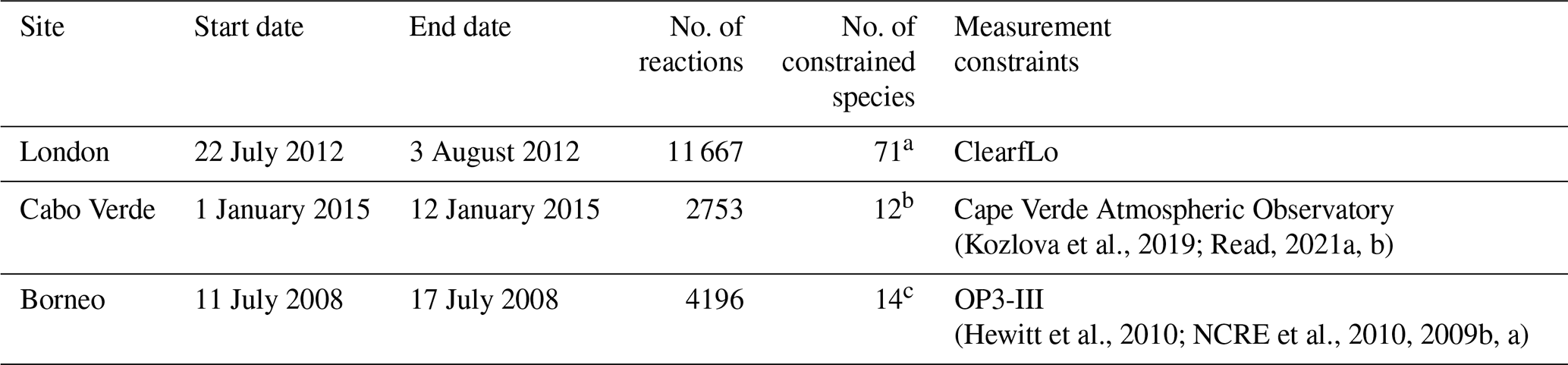
The current version of the mechanism, MCM v3.3.1, accounts for the degradation of 142 volatile organic species and involves around 17 000 elementary reactions (Rickard and Young, 2018). For this work, MCM v3.3.1 was implemented in the open-source box model AtChem V1.2 (Sommariva et al., 2020). The box modeling aimed to determine which aldehydes contribute meaningfully to the primary chemical production of H₂ in different types of environments. We chose three indicative sites to explore distinctive environments, each with different expected mixing ratios of aldehydes (urban, pristine oceanic and pristine forested). The direct production of H₂ from the photolysis of aldehydes evaluated with AtChem further helped to configure the global model (see Sect. 3.3). For each site, the model was configured with different subsets of the MCM that were downloaded for selected species based on the measurements available to constrain the box model. Likewise, the length of each simulation was set based on the dates for which measurements were available to constrain the box model.

Table 1 contains a summary of the box model simulations. The first box model simulation was run for London, with 71 chemical species constrained by the measurements from the ClearfLo (Clean Air for London) campaign of 2012 (Bohnenstengel et al., 2015). The measurements to constrain the box model for London were previously used by Shaw et al. (2018) to test the formation of formic acid from the photo-tautomerization of acetaldehyde. The box model for London considered 11 667 reactions for 3880 species. The second model simulation was configured for Cabo Verde. The measurements used to constrain the model were those from the Cape Verde Atmospheric Observatory, located in the tropical Atlantic marine boundary layer. A total of 12 species were constrained from measurements taken in January 2015 (Kozlova et al., 2019; Read, 2021a, b). This box model setup included 2753 reactions for 894 species. The third box model simulation was conducted for the southeast Asian tropical rainforest in Borneo. The measurements of 14 species from the OP3-III campaign at Bukit Atur, Sabah, Malaysia (Hewitt et al., 2010) were used as constraints. For the third box model simulation, the subset of the MCM contained 4196 reactions for 1356 species. All three models included a total of 18 aldehydes (see Table S1 in the Supplement) with their corresponding reactions. Of these, only two (formaldehyde and glyoxal) already included H₂ as a photolysis product in the standard MCM v3.3.1 mechanism.

An initial baseline using the standard MCM v3.3.1 was simulated to use for later comparison against four sets of sensitivity tests. All simulations were initialized with an H₂ abundance of 1.30×10¹³ molec. cm⁻³ (∼530 ppbv). The value was chosen based on the average H₂ mixing ratios from four measuring sites located across the world (Krummel et al., 2021b, a, d, h). The four sensitivity tests were designed to explore the relative contribution that the photolysis of aldehydes could have on the chemical production and resultant mixing ratios of H₂. To that end, new photochemical channels were added for 16 aldehydes available in the extracted MCM subsets (see Table S1), with H₂ specified as a primary product. Previous experimental findings have demonstrated H₂ quantum yields that varied from 1 % for acetaldehyde (Harrison et al., 2019) to 8 % for methylpropanal (Kharazmi, 2018). Consequently, the four box model tests used uniform 1 %, 2 %, 5 % and 10 % quantum yields across all 16 available aldehydes and across all wavelengths, with the goal of bracketing the plausible range of behavior. We did not include physical processes in the box modeling, as the goal of these simulations was to explore the contribution to H₂ from aldehyde photolysis relative to the other chemical sources and sinks. This means that the box models do not consider either direct emissions or the soil uptake sink of H₂. Furthermore, the soil uptake is not relevant at this stage because of the timescale in which we conducted the simulations.

(Kozlova et al., 2019; Read, 2021a, b)(Hewitt et al., 2010; NCRE et al., 2010, 2009b, a)

Table 1 Summary of the box model configurations.

^a 1-Butanal, 1-butene, 1-pentene, 1-propanol, 1,2-dimethylethylene, 1,3-butadiene, 2-butene, ethyne, 2-ethyltoluene, 2-hexanone, 2-methylbutane, 2-methylpentane, 2-methylpropanal, 2-pentanone, 3-ethyltoluene, 4-ethyltoluene, 4-methyl-2-pentanone, acetaldehyde, acetone, α-pinene, benzaldehyde, benzene, butanal, butane, CO, cyclohexanone, decane, dodecane, ethane, ethanol, ethene, ethyl acetate, ethylbenzene, formaldehyde, hemimellitene, heptane, hexane, isobutane, isobutene, isoprene, isopropylbenzene, limonene, m-xylene, mesitylene, methacrolein, methane, methanol, methyl ethyl ketone, methyl vinyl ketone, methylene chloride, nitric acid, NO, NO₂, nonane, o-xylene, octane, ozone, p-xylene, pentanal, pentane, peroxyacetyl nitrate, propane, propene, propylbenzene, pseudocumene, styrene, toluene, trans-2-pentene, trichloroethylene, undecane, H₂O. ^b 2-Methylbutane, butane, ethane, ethene, isobutane, methane, ozone, pentane, propane, propene, toluene, benzene. ^c 1-Butene, acetaldehyde, acetone, α-pinene, ethene, ethyne, formaldehyde, limonene, methacrolein, methanol, NO₂, isoprene, ozone, propene.

The individual photolysis rates for the new aldehyde photolysis reactions were calculated and incorporated into each box model simulation as constrained values at each site. The calculation of the photolysis rates (J) for each aldehyde followed the Eq. (1):

$$\begin{array}{}\text{(1)}& J=\underset{\mathit{\lambda }\mathrm{1}}{\overset{\mathit{\lambda }\mathrm{2}}{\int }}F\left(\mathit{\lambda }\right)\mathit{\varphi }\left(\mathit{\lambda }\right)\mathit{\sigma }\left(\mathit{\lambda }\right)d\mathit{\lambda },\end{array}$$

where λ1 is 290 nm, λ2 is 345 nm, F is the actinic flux as a function of the zenith angle, σ is the cross section of each aldehyde and ϕ is the quantum yield, varied as explained previously (1 %, 2 %, 5 % and 10 %). Table S1 lists the aldehydes available in MCM that were used in the model sensitivity experiments, along with the corresponding photolysis products and reaction rates calculated using Eq. (1). For the reactions where H₂ is produced partnered to a ketene molecule, glycolaldehyde was used as a surrogate species for ketene as neither MCM nor GEOS-Chem include ketene in their mechanisms.

2.2 Box modeling results: contributions of aldehydes to the photochemical production of H₂

Because of the short modeled times (limited by available measurement constraints), none of the baseline simulations represented steady-state conditions. As a result, we focus on interpretation of changes to chemical production rather than changes to mixing ratios. For a brief discussion on the mixing ratios obtained in the box modeling, see the Supplement.

H₂ chemical production provides a more realistic and useful outcome from the box model simulations. At all three modeled sites, the relative rate of H₂ chemical production in the sensitivity simulations increases relative to the baseline simulation and scales linearly with the quantum yield over the 1 %–10 % range studied here (see Figs. S4 and S5). This linearity makes it reasonable to interpolate the predicted MCM production rates simulated here for as-yet unmeasured aldehydes to whatever experimental quantum yield is ultimately determined.

We use the sensitivity simulations to evaluate the relative importance of each aldehyde. Figure 1 displays the relative daytime contribution of each newly considered aldehyde to the total aldehyde-derived photolysis H₂ production rates modeled using a 1 % quantum yield (not including the contributions from formaldehyde and glyoxal, which were not modified in this work). To aid the eye, aliphatic aldehydes are grouped in orange tones, unsaturated aldehydes (and methylglyoxal) in green tones and oxygenated aldehydes in blue tones. For the London site, aliphatic aldehydes (orange) dominated, with acetaldehyde by far the largest contributor (74 %). The remaining contributions were distributed between propanal (12 %), methylglyoxal (5 %), glycolaldehyde (5 %), and to a lesser extent acrolein and methacrolein. The contribution of biogenic-related species in London like methylglyoxal, glycolaldehyde and methacrolein can likely be attributed to the presence of isoprene, which reached a maximum value of ∼400 pptv ($\sim \mathrm{1.0}\times {\mathrm{10}}^{\mathrm{10}}$ molec. cm⁻³) as shown in Fig. S1 in the Supplement.

While six species contributed to the modeled production of H₂ from aldehydes at London, at the Cabo Verde site just three aldehydes were dominant. Aliphatic aldehydes, mostly acetaldehyde (72 %) and propanal (18 %), again dominated H₂ production, with an additional contribution from methylglyoxal (10 %). There was virtually no contribution from any other aldehyde.

For Borneo, the modeled distribution of the aldehyde contributions to H₂ production was completely different than modeled at the other two sites. Aliphatic aldehydes provided only a minor contribution. There was a particularly notable difference in the influence of acetaldehyde, which represented more than half the new H₂ production at London and Cabo Verde but only 5 % of the production at Borneo. Meanwhile, the contributions of methylglyoxal (46 %), glycolaldehyde (35 %) and other unsaturated aldehydes were markedly larger at Borneo than at the other two sites. The results for Borneo clearly show the influence of biogenic isoprene in the rainforest atmosphere, as methylglyoxal, glycolaldehyde and methacrolein are all products of isoprene oxidation (Wennberg et al., 2018). The isoprene in Borneo reached values of up to 2350 pptv (5.7×10¹⁰ molec. cm⁻³) (Hewitt et al., 2010) (see Fig. S3). As a comparison, the isoprene mixing ratios in London were much lower at about ∼17 % of the Borneo values. No isoprene was simulated for Cabo Verde, but previously reported typical noon values at Cabo Verde of ∼10 pptv (Whalley et al., 2010) imply its contribution to H₂ production from aldehydes there would be negligible. The larger effect of the new photochemical H₂ sources at Borneo relative to the other sites due to the abundance of biogenic VOCs implies the newly discovered photochemical production pathways will have most influence in biogenic source regions, and this will be explored in the next section using the global model.

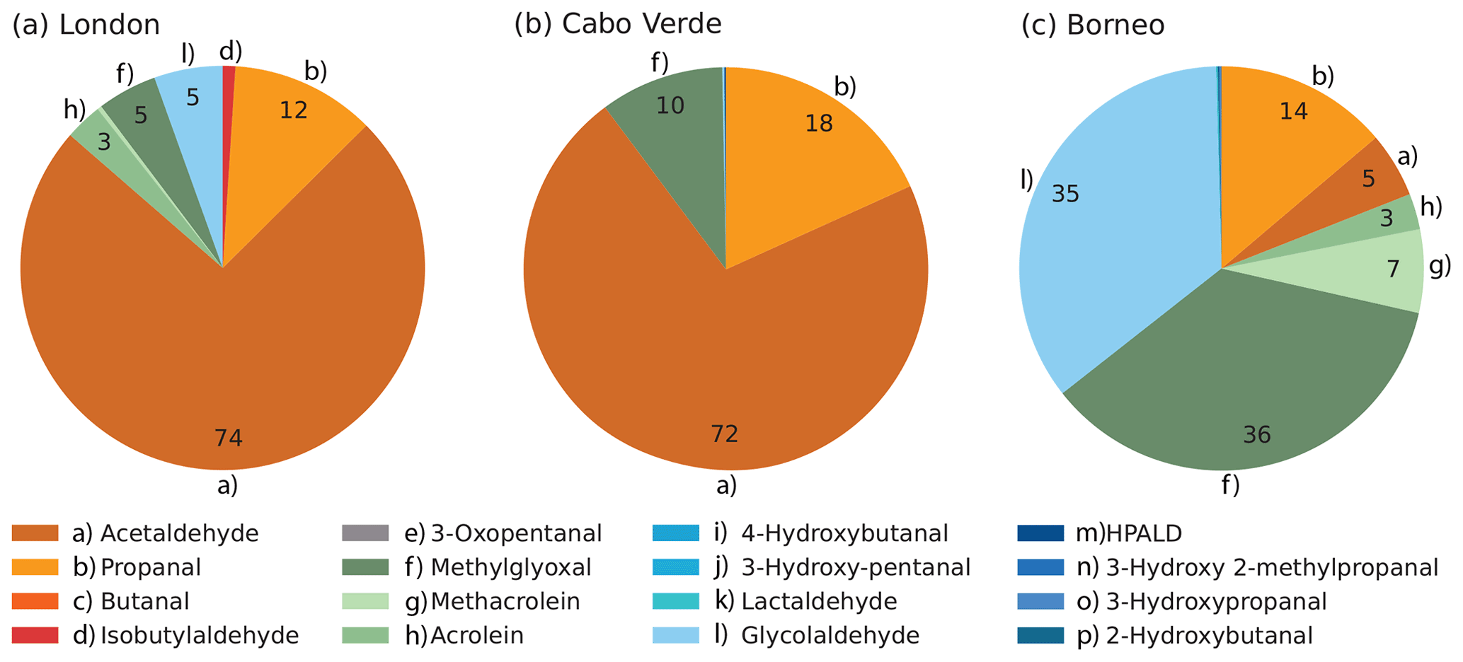
Figure 1 Average daytime percentage contribution of individual aldehydes to the total production of H₂ from aldehydes (excluding formaldehyde and glyoxal) assuming a 1 % quantum yield, estimated for the (a) London, (b) Cabo Verde and (c) Borneo sites using the box model. The daytime average H₂ rates of production from all aldehydes (including formaldehyde and glyoxal) were 6.35×10⁶ molec. cm⁻³ s⁻¹ for London, 6.45×10⁵ molec. cm⁻³ s⁻¹ for Cabo Verde and 6.64×10⁵ molec. cm⁻³ s⁻¹ for Borneo. These rates were calculated for the length of the simulation at each site (see Table 1).

The box modeling with the MCM v3.3.1 allowed us to test H₂ production from the photolysis of a wide range of aldehydes in a complex and explicit chemical mechanism. While H₂ did not reach steady state in any of the box models (due to the short simulation period), these box model simulations identified the aldehydes that are expected to contribute the most to photolytic production of H₂ under distinct environmental conditions. In urban environments, modeled as the London site, linear aliphatic aldehydes (especially acetaldehyde and propanal) are the most relevant. For regions with substantial vegetation (e.g., tropical forested areas such as Borneo), aldehydes that are produced from the oxidation of isoprene, such as methylglyoxal and glycolaldehyde, are the most important. At all three sites, aside from glycolaldehyde, none of the oxygenated aldehydes modeled here (blue tones in Fig. 1) featured any significance to the formation of H₂. The aggregated rate of production from the tested aldehydes here was less than 1 % of the total rate of production at each modeled site, with formaldehyde and glyoxal remaining the main photochemical sources of H₂ in the box model simulations. However, the short simulation times (driven by lack of appropriate observational constraints) and the absence of physical sources and sinks limit the usefulness of the box model results for further quantifying the effects of the relevant identified aldehydes on tropospheric photochemical formation of H₂. We therefore turned to a global chemical transport model (GEOS-Chem), in which we were able to include not only the new photochemistry for the most relevant species as identified by the box modeling but also physical processes (emissions and soil uptake). With the global model, we were also able expand the evaluation to diverse environments across the globe and to run simulations for periods long enough to allow H₂ to reach steady state, providing more robust results. The global modeling of H₂ is described in the following section.

3 Global atmospheric modeling of H₂ using GEOS-Chem

3.1 GEOS-Chem model configuration: development of the baseline simulation of H₂.

GEOS-Chem is a widely used 3-D chemical transport model originally described by Bey et al. (2001). The current work used version 12.5.0 modified to include H₂ as part of the standard chemistry simulation. To test the production of H₂ from aldehydes with the atmospheric model, we first constructed a baseline simulation that included all other known H₂ sources and sinks. All GEOS-Chem simulations were performed on a $\mathrm{4}{}^{\circ }\times \mathrm{5}{}^{\circ }$ horizontal resolution with 72 vertical layers. The simulations included stratospheric chemistry using the UCX mechanism (Eastham et al., 2014) and were driven by Goddard Earth Observing System Forward Processing (GEOS-FP) meteorology from the Global Modeling and Assimilation Office (GMAO). The default version of GEOS-Chem v12.5.0 does not include H₂ as an active species, and so the H₂ mixing ratio has a fixed concentration of 500 ppbv across the troposphere. However, observations compiled by CSIRO at four sites, two located in the Northern Hemisphere (Krummel et al., 2021b, a) and two in the Southern Hemisphere (Krummel et al., 2021d, h), show that on average the global mixing ratio of H₂ is ∼530 ppbv. Based on these observations, the initial mixing ratio of H₂ was modified in GEOS-Chem to match the average observed value of 530 ppbv (to reduce spin-up time). We ran a 6-month spin-up from June to December 2014 and verified that the model had achieved steady state at that point. Tests with 18-month and 2.5-year spin-ups showed differences in H₂ mixing ratios were smaller than 0.5 %, showing that the 6-month spin-up was sufficient. The baseline simulation was then run from January 2016 to December 2016.

For our baseline configuration, we added known H₂ physical sources and sinks into GEOS-Chem. We scaled H₂ anthropogenic emissions to inventory estimates of carbon monoxide (CO) emissions as done previously in other studies (Ehhalt and Rohrer, 2009) as there are no dedicated emission inventories available for H₂. The scaling was performed using the Harmonized Emissions Component (HEMCO) in GEOS-Chem (Lin et al., 2021). Two different emission ratios were implemented for anthropogenic combustion sources, one for general use of fossil fuels (0.042 g H₂ g⁻¹ CO) based on the fraction used by Price et al. (2007) and the other for automobile emissions (0.036 g H₂ g⁻¹ CO) based on the fraction used by Ehhalt and Rohrer (2009).

For the anthropogenic H₂ emissions, the Community Emissions Data System (CEDS) global inventory (Hoesly et al., 2018) was used. The CEDS emissions were overwritten by more detailed regional emission inventories where applicable: APEI for Canada, DICE-Africa for Africa (Marais and Wiedinmyer, 2016), EPA/NEI11 for North America and MIX for East Asia (Li et al., 2017). For the biomass burning H₂ emissions, the Global Fire Emissions Database v4 (GFEDv4s) (Randerson et al., 2018) was used. We used biome-specific H₂ emission factors from Andreae (2019) and Akagi et al. (2011). The emission factors used were 1.2 g kg⁻¹ for peat fires; 2.6 g kg⁻¹ for agricultural waste burning; 3.1 g kg⁻¹ for deforestation (tropical) and degradation; 1.6 g kg⁻¹ for boreal forest fires; 2.1 g kg⁻¹ for temperate forest fires; and 1.7 g kg⁻¹ for savanna, grassland, and shrubland fires. Oceanic emissions were from Price et al. (2007), who distributed reference H₂ emissions of 6 Tg yr⁻¹ globally using the spatial distribution of biological nitrogen fixation in the ocean determined by Deutsch et al. (2007). The simulation also uses the Model of Emissions of Gases and Aerosols from Nature, MEGANv2.1 (Guenther et al., 2012), for biogenic emissions of volatile organic compounds, several of which are the aldehydes that are included in this work as sources of H₂.

Figure 2a shows the average annual global primary sources of H₂ for 2015 and 2016 from biomass burning, oceanic and anthropogenic emissions (all in Tg yr⁻¹). The red pixels in Fig. 2a show that China contributes the most to the emissions of H₂ due to the large anthropogenic sources there. Biomass burning emissions from the African savannas, Indonesia, the Amazon, and some parts of North America and Russia are important sources of molecular H₂ but to a lesser extent than the anthropogenic emissions. Oceanic H₂ sources show maximum emissions occurring over the Pacific with no emission at high latitudes (poleward of 40^∘ S and 40^∘ N), as described in detail by Price et al. (2007).

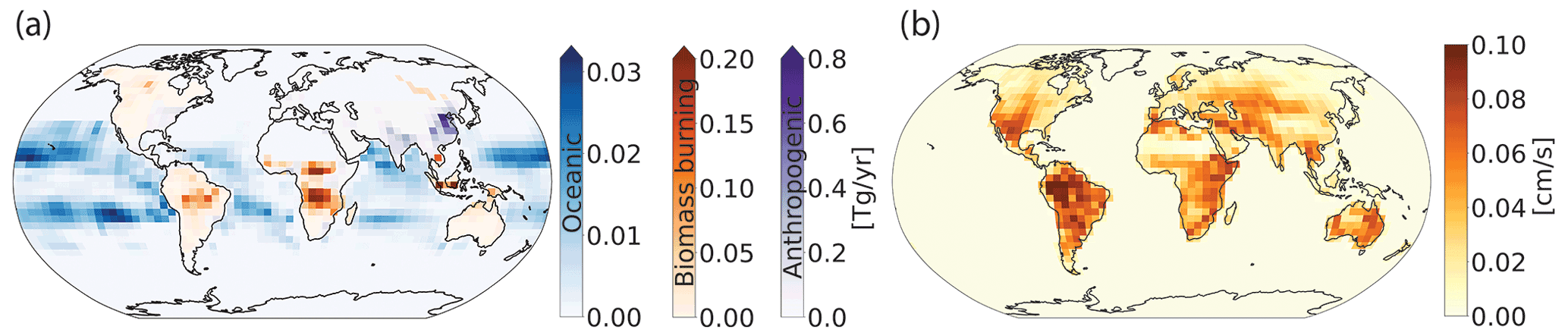
Figure 2 (a) Average annual global emissions of H₂ in Tg yr⁻¹ from 2015 and 2016 from biomass burning (red), oceanic (blue) and anthropogenic (purple) sources. Anthropogenic emissions include fossil fuel and biofuel combustion. Note the difference in scales for the different source types. (b) Average annual dry deposition velocity of H₂ in centimeters per second (cm s⁻¹) supplied into GEOS-Chem and determined from the original calculations from Yashiro et al. (2011).

We also added the atmospheric H₂ sink from soil uptake. The soil uptake of H₂ involves both biological (enzymatic and microbial activity) and physical (molecular diffusion) processes, which jointly determine the magnitude of the sink (Yver et al., 2011). The correlation of the enzymatic and microbial activity with soil temperature and moisture drives the seasonality of atmospheric H₂. Soil temperatures between 20 and 30 ^∘C are optimal to capture H₂, with no capture below −20 ^∘C or above 40 ^∘C. Likewise, arid and frozen soils have been shown to have low values of H₂ uptake (Yashiro et al., 2011). The rate of soil uptake of H₂ has been measured as a dry deposition velocity and thus is typically parameterized in models as a dry deposition process (Ehhalt and Rohrer, 2009; Yver et al., 2011; Yashiro et al., 2011). Reported values of dry deposition velocities of H₂ onto soils range from 0.01 to 0.15 cm s⁻¹ based on measurements in savanna, tundra, and desert ecosystems and in agricultural lands (Ehhalt and Rohrer, 2009).

Although GEOS-Chem is capable of calculating the dry deposition velocities using a resistance-in-series scheme that relies on known parameters (including Henry's Law constants and reactivity factors, among others), we instead used offline dry deposition velocities derived from a comprehensive soil H₂ model developed by Yashiro et al. (2011). The integration of an online H₂ dry deposition calculation from other studies (Yashiro et al., 2011; Ehhalt and Rohrer, 2013; Bertagni et al., 2021) was not performed given that the algorithms require soil variables (e.g., soil porosity, soil moisture, soil temperature and depth of soil active layers) that are not available in the post-processed GEOS-FP meteorological fields used as input to GEOS-Chem. However, the variables are available in the raw GEOS-FP (and MERRA-2) dataset. Future work should explore processing these variables for use in GEOS-Chem and implementing online soil uptake into the model. To calculate the dry deposition velocities used here, Yashiro et al. (2011) used a two-layered diffusion/uptake model that considers biologically inactive (where no H₂ uptake takes place) and active layers as well as the porosity, temperature and moisture of the soil. The Supplement contains the detailed equations used by Yashiro et al. (2011) to obtain the dry deposition velocities used here, along with a brief description of the differences between the (Yashiro et al., 2011) parameterization and the (Ehhalt and Rohrer, 2013) parameterization applied in other recent modeling studies (Paulot et al., 2021).

Yashiro et al. (2011) provide highly resolved values of the dry deposition velocity of H₂, derived from a total of 8 modeled years (1997–2005) with daily resolution on a $\mathrm{1.25}{}^{\circ }\times \mathrm{1.25}{}^{\circ }$ horizontal grid with global coverage. We used the dry deposition velocities from Yashiro et al. (2011) to create a climatology for an average year with daily temporal resolution to represent typical seasonal variability, which was then used in our 2014–2016 simulations. The $\mathrm{1.25}{}^{\circ }\times \mathrm{1.25}{}^{\circ }$ resolution dry deposition velocities of H₂ were mapped to our modeled grid ($\mathrm{4}{}^{\circ }\times \mathrm{5}{}^{\circ }$) using HEMCO.

Figure 2b shows the annual average H₂ dry deposition velocities gridded as used in GEOS-Chem. The dry deposition velocities ranged from 0.1 to 0.10 cm s⁻¹. Regions like the Sahara desert and far eastern Russia have the lowest dry deposition velocities because the uptake efficiencies are diminished by the extremely high or low soil temperatures and moisture content (Yashiro et al., 2011), which inhibit H₂ capture as described previously. Equatorial regions have the highest dry deposition velocities, and in these regions they remain almost constant throughout the year.

Deposition onto water bodies is not considered in our simulations. Although Punshon et al. (2007) provide first-order net loss-rate constants of H₂ in seawater sampled in Canada, these values have not been extensively tested, and it is unclear whether they are broadly representative of other waters. Further, the loss rates are not well known under different conditions (e.g., salty tropical waters versus freshwater lakes). Ehhalt and Rohrer (2009) suggested that the deposition of H₂ onto water is at most a minor player in the tropospheric budget of H₂. Considering this finding and the lack of extensive research on loss of H₂ to water bodies, we did not include this sink and expect this would have a negligible impact on the findings reported here.

Our baseline simulation also includes H₂ chemical production and loss. The standard chemical mechanism in GEOS-Chem already includes the major known chemical sources of H₂: photolysis of formaldehyde and glyoxal, reaction of excited oxygen atoms with methane, and reaction of the H atom with the hydroperoxyl radical. Similarly, the standard mechanisms also include the only known significant chemical H₂ sinks: reaction of H₂ with the hydroxyl radical and with chlorine atoms. While these sources and sinks were already present in GEOS-Chem v12.5.0, they did not influence simulated H₂ as it was set as a “fixed” species, with a constant value of 500 ppbv. Here we change H₂ to an active species so that the H₂ concentrations change in response to the chemical sources and sinks outlined above.

3.2 GEOS-Chem modeling results: evaluation of the baseline simulation

Before testing the impact of the new H₂ source from aldehyde photolysis, we first evaluated the performance of the baseline simulation. Table 2 summarizes the burden, lifetime and tropospheric budget of H₂ calculated for our baseline simulation, along with values from previous research. Using our new GEOS-Chem baseline configuration, we calculated the global burden of H₂ to be 157.8 Tg for 2015 and 157.6 Tg for 2016. These estimated values are within the range of previous reports of the global burden of H₂, which ranged from 136 Tg (Hauglustaine and Ehhalt, 2002) to 172 Tg (Sanderson et al., 2003). Our estimate for the H₂ lifetime is 2 years, in agreement with previous reports that range from 1 year (Rhee et al., 2006; Xiao et al., 2007) to 2.3 years (Sanderson et al., 2003).

Novelli (1999)Hauglustaine and Ehhalt (2002)Sanderson et al. (2003)Rhee et al. (2006)Price et al. (2007)Xiao et al. (2007)Ehhalt and Rohrer (2009)Yver et al. (2011)Yashiro et al. (2011)Derwent et al. (2020)Paulot et al. (2021)

Table 2 Global tropospheric sources (Tg yr⁻¹), sinks (Tg yr⁻¹), burdens (Tg) and lifetimes (yr) of H₂.

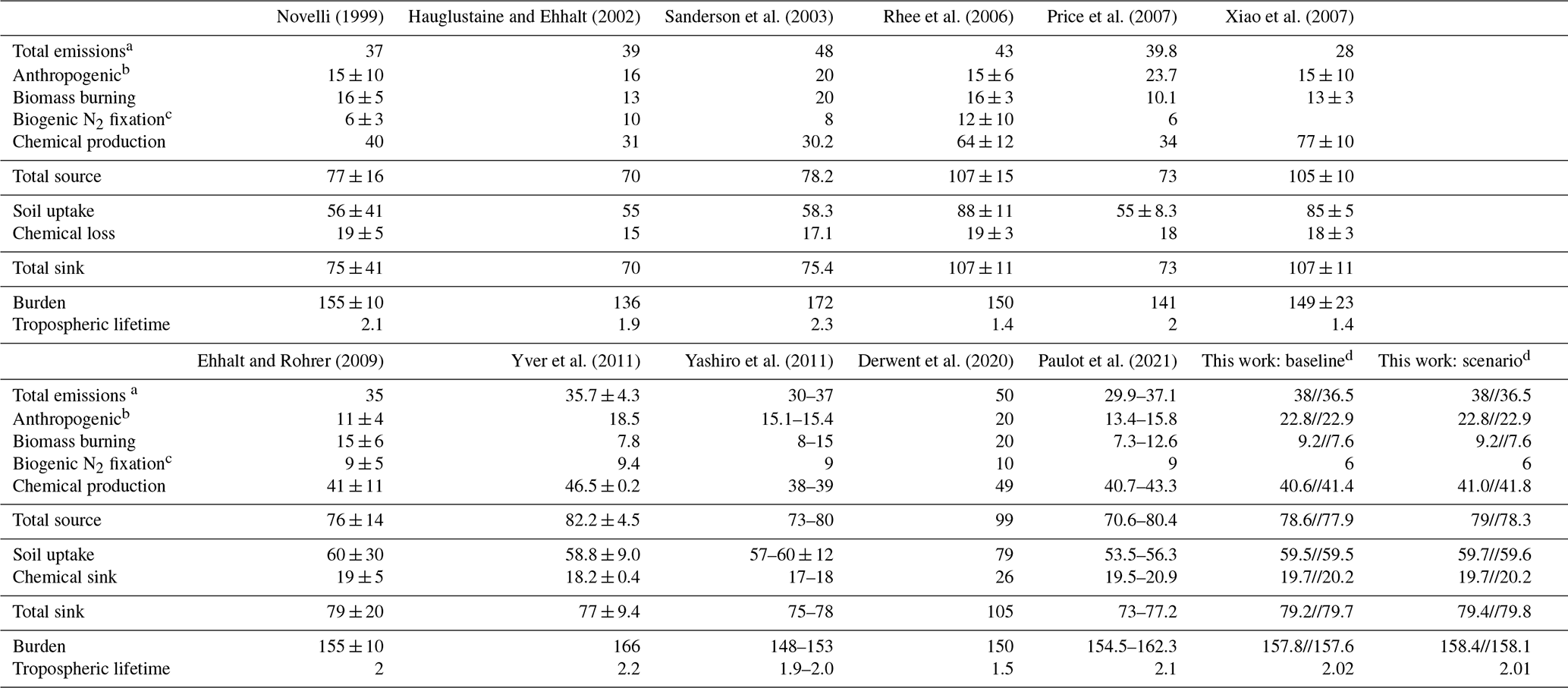
^a Includes anthropogenic (fossil fuel), biomass burning and biogenic N₂ fixation emissions. ^b Includes fossil-fuel- and biofuel-related emissions. ^c Includes land and ocean N₂ fixation emissions. ^d Budgets are reported for 2015//2016.

Compared against other studies, anthropogenic emissions are one of the highest with 22.8 Tg yr⁻¹ for 2015 and 22.9 yr⁻¹ for 2016. Biomass burning emissions in our simulations were amongst the lowest estimates, with 9.2 Tg yr⁻¹ for 2015 and 7.6 Tg yr⁻¹ for 2016, compared to other estimates that ranged from 8 Tg yr⁻¹ (Yashiro et al., 2011) to 20 Tg yr⁻¹ (Derwent et al., 2020). We expect the discrepancy comes either from interannual variability between the different modeled years or from differences in the underlying emissions inventories. For the latter, most studies did not specify the inventory used for biomass burning; however, previous work has shown that there can be large differences between inventories, including GFEDv4s as used here (Desservettaz et al., 2021; Liu et al., 2020). Ocean emission estimates are within the reported values at 6 Tg yr⁻¹.

Chemical production of H₂ in our baseline simulation was 40.6 Tg yr⁻¹ for 2015 and 41.4 Tg yr⁻¹ for 2016, within the range from most recent studies of 30 Tg yr⁻¹ (Sanderson et al., 2003) to 49 Tg yr⁻¹ (Derwent et al., 2020). Earlier estimates of 64 ± 12 yr⁻¹ from Rhee et al. (2006) and 77 ± 10 Tg yr⁻¹ from Xiao et al. (2007) are higher than all other estimates, a difference that Ehhalt and Rohrer (2009) have attributed to their use of top-down inverse methodology, as opposed to the bottom-up approach used in other studies (including our baseline). The generally good agreement in the H₂ chemical source between our baseline and the other studies indicates that photolysis of formaldehyde and glyoxal yields H₂ production consistent with prior estimates, providing an appropriate baseline to compare to the so far unexplored photochemical production of H₂ from other aldehydes.

As in previous work, the soil uptake sink was almost 3 times higher than the chemical sink in our baseline simulation. We simulated a soil uptake sink of ∼60 Tg yr⁻¹ which fell within the range reported by Yashiro et al. (2011), the source of the H₂ dry deposition velocities used here. Most other studies also show a similar soil uptake sink, with a few exceptions as described in detail by Yashiro et al. (2011). The chemical sink in our baseline simulation was ∼20 Tg yr⁻¹, again consistent with all other studies. The strength of the soil uptake sink varied throughout the year, while the chemical sink was largely stable (Fig. 3c, d). In general, the tropospheric burden, budget and lifetime of H₂ determined using our baseline compared well with previous references.

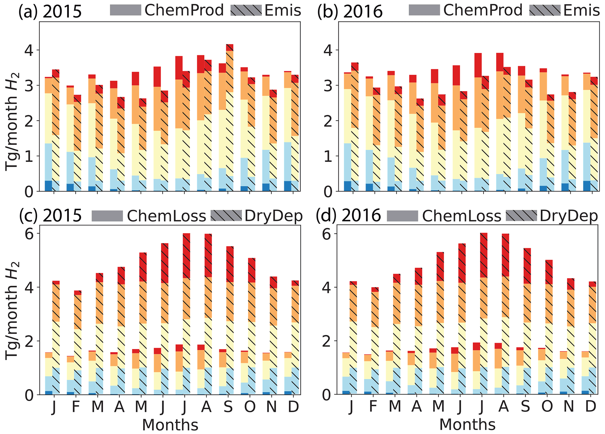
Figure 3 Simulated global monthly H₂ sources (a, b, chemical production (solid) and emissions (hashed)) and sinks (c, d, chemical losses (solid) and dry deposition(hashed)) for 2015 (left: a, c) and 2016 (right: b, d), calculated using the GEOS-Chem baseline simulation. Both sources and sinks are aggregated by latitudinal band as follows: red – high Northern Hemisphere (HNH) north of 45^∘ N; orange – lower Northern Hemisphere (LNH) from 15 to 45^∘ N; yellow – tropics (TP) from 15^∘ S to 15^∘ N; light blue – lower Southern Hemisphere (LSH) from 15 to 45^∘ S; dark blue – high Southern Hemisphere. The emissions (Emis) include anthropogenic, biomass burning and biogenic N₂ fixation sources. The chemical production (ChemProd) includes photochemical formation from formaldehyde and glyoxal. The chemical loss (ChemLoss) considers the reaction with OH. The dry deposition (DryDep) is also shown.

We evaluated the modeled mixing ratios of H₂ from the baseline simulation using CSIRO measurements reported by Krummel et al. (2021b, c, d, e, f, g, h, a) and a measurement site reported by AGAGE (Wang et al., 2021). The CSIRO datasets correspond to monthly flask air sample measurements of H₂ (along with CO₂, CH₄, CO, N₂O, and ¹³C and ¹⁸O isotopes of CO₂) at eight ground-based sites with data from 1992 to 2019 and all include measurements for 2015 and 2016, plus one set of H₂ aircraft measurements with data from 1991 to 2000. Six of the ground sites in this dataset are located in the Southern Hemisphere, with the remaining two sites in the Northern Hemisphere. The measuring site from AGAGE is located in the Northern Hemisphere. Both CSIRO and AGAGE data are reported in the MPI-2009 scale (Jordan and Steinberg, 2011).

Previous work has compared modeled H₂ against measurements by the National Oceanic and Atmospheric Administration (NOAA) Earth System Research Laboratory (ESRL) (Price et al., 2007; Ehhalt and Rohrer, 2009; Yashiro et al., 2011). The NOAA dataset provides around 125 measuring sites with H₂ measurements across the world starting from 1989 (Dlugokencky et al., 2017). However, the NOAA data are subject to calibration issues that remain unresolved (Masarie et al., 2001). CSIRO data, supported by a more robust calibration scheme, are used for this study despite having lower spatial coverage of measurement sites.

We use the CSIRO measurements (Krummel et al., 2021a, b, c, d, e, f, g, h, i) and the AGAGE measurements at Mace Head in Ireland (Wang et al., 2021) to assess the H₂ seasonal cycles. Model biases and other statistical metrics calculated are shown in Table S2.

Figure 4 shows a seasonal spatial average of H₂ mixing ratios in surface air averaged over 2015 and 2016, with simulated values overlaid by the observations of CSIRO. Modeled mixing ratios at 500 hPa can be seen in Fig. S6. As expected, in each hemisphere, the H₂ mixing ratios are lower in the corresponding summer and autumn than in spring and winter months. This seasonal trend is driven by the soil uptake (Fig. 3) and its relationship with soil temperature and moisture. During summer and autumn, the temperature conditions are optimal for the soil uptake of H₂, yielding lower concentrations of H₂ in surface air.

In the Northern Hemisphere, the mixing ratios of H₂ were highest during the December–January–February (DJF) and the March–April–May (MAM) periods. Modeled H₂ was lowest in SON over Russia (∼400 ppbv), followed by North America (∼450 ppbv). The high modeled mixing ratios over China and Korea (∼600 ppbv) remained almost constant throughout the year, consistent with high emissions from anthropogenic combustion sources (see Fig. 2). The season with the highest modeled estimates of H₂ over China and Korea is DJF. A similar trend in the estimated mixing ratios of CO implies that the anthropogenic emissions inventories used over this region are likely responsible for the high values of these modeled gases.

In the Southern Hemisphere, elevated H₂ mixing ratios on the order of 550–600 ppbv modeled over Africa and Indonesia in austral winter–spring (JJA and SON) coincide with the seasonal cycle of biomass burning emissions (Pak et al., 2003; Edwards et al., 2006). Throughout the year, the lowest H₂ mixing ratios globally are found in South America, in particular in the Amazon region. Over these regions, modeled mixing ratios are consistently lower than 450 ppbv. To our knowledge, there are no available measurements of H₂ for South America that could be used to evaluate the modeled mixing ratios there. Observations are also lacking over most of the Middle East, parts of Asia, Africa and Australia. H₂ measurements over these regions would provide particularly valuable constraints in further modeling endeavors.

The visual comparisons in Fig. 4 show that there are different biases in different locations, with notable underestimates at the Southern Hemisphere observing sites. The Supplement includes a comparison of average modeled and observed H₂ vertical profiles using historic (1991–2000) aircraft measurements (Krummel et al., 2021i). These are shown in Figure S7. For the vertical profile comparison of the H₂, we used the records from the aircraft (AIA) flask sampling data from Krummel et al. (2021i) measured over Tasmania. The seasonal average ratios of the H₂ measured at varying heights with respect to the surface values (from 1991 to 2000) were plotted against the average model estimates from 2015 and 2016 (see Fig. S7). SON and DJF were the seasons during which GEOS-Chem represented best the evolution of H₂ with altitude. On the other hand, for MAM and JJA, the model was unable to capture the vertical gradient of the observations attributing more H₂ in height than the reported in the average 9-year trend. This might be caused by enhanced modeled vertical transport of H₂, but this is difficult to determine with this limited dataset.

While limited in spatial extent, the CSIRO data are well suited for evaluating modeled mixing ratios and seasonal patterns. Figure 5 compares monthly mean modeled mixing ratios of H₂ against measurements at the sites from the CSIRO and AGAGE ensemble for 2015 and 2016 (Krummel et al., 2021a, b, c, d, e, f, g, h; Wang et al., 2021). At the three sites located in the Northern Hemisphere (Alert, ALT; Mace Head, MHD; and Mauna Loa, MLO), GEOS-Chem was able to capture both the magnitude and the majority of the variability over the 2 years. At the six sites in the Southern Hemisphere (Cape Ferguson, CFA; Cape Grim, CGO; Macquarie Island, MQA; Casey, CYA; Mawson, MAA; and South Pole, SPO), the model captures the observed seasonality but is biased low by $>\sim \mathrm{20}$ ppbv. In other words, the CSIRO measurements indicate a persistent low bias in modeled Southern Hemisphere H₂ mixing ratios. The measurements at sites like Cape Grim (CGO) represent baseline-selected (clean air masses) only. The model output analyzed was not filtered to match background conditions at some of the CSIRO sites, a condition that could be a minor contributing factor to some of the observed bias. Figure S8 shows that the baseline-selected in situ data have differences of ∼3 ppb and are in good agreement with baseline-sampled flask data. We do not expect the oxidation of CH₄ to be a possible source of our H₂ model bias because CH₄ is constrained to observations at the surface in our simulations. A misrepresentation of biomass burning emissions or biased inter-hemispheric modeled mixing ratios is also unlikely to be the cause of the difference between observations and model simulations because of the good model performance shown in CO estimates. However, a revision of the mass fractions used to scale the emissions inventories of CO to H₂ is recommended. Figure S9 in the Supplement shows that the Southern Hemisphere modeled bias is unique to H₂ and is not seen in CO. Given the large ocean area in this part of the world, underestimated ocean H₂ emissions are a possible driver of the bias, although we did not estimate the magnitude of the emissions that is required to overcome such bias. Improvements to ocean H₂ emission parameterizations with particular emphasis on the Southern Ocean should be a priority for future model development.

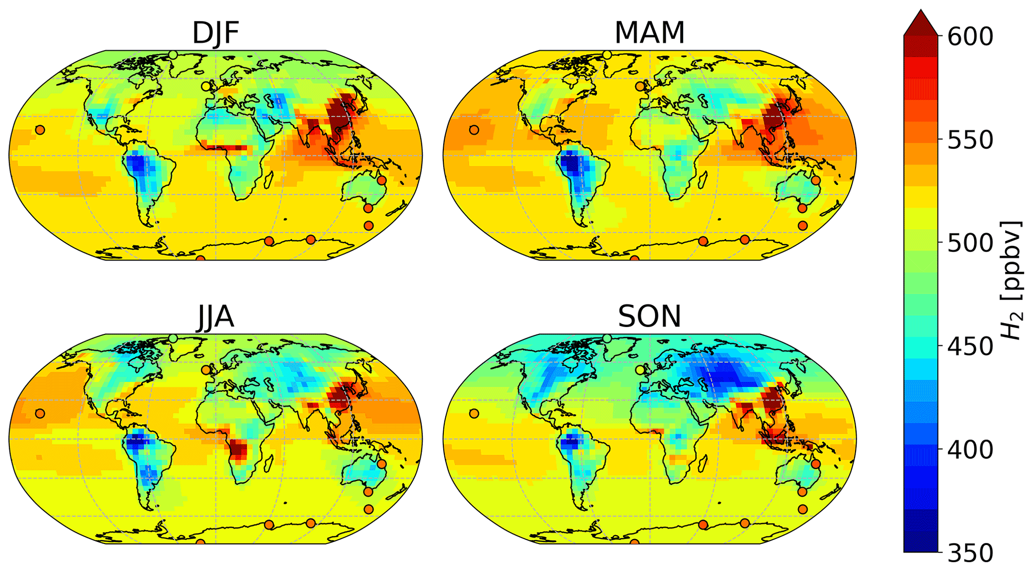
Figure 4 Average surface air H₂ mixing rations in each season as estimated by the GEOS-Chem baseline simulation (background), compared against average measured values from CSIRO (circles). Both modeled and observed values have been averaged over 2015–2016.

Overall, our baseline model was able to capture the main features of observed spatial and seasonal variability of the H₂ reported by CSIRO and AGAGE (Krummel et al., 2021b, c, d, e, f, g, h, a; Wang et al., 2021). Combined with the fact that the simulated H₂ budget, burden and lifetime are all consistent with previous estimates, the observational evaluation lends confidence to the suitability of our baseline model configuration. In what follows, we further adapt our baseline configuration to test the impact on tropospheric H₂ of its generation from photolysis of aldehydes other than formaldehyde and glyoxal.

3.3 GEOS-Chem modeling results: global implications of H₂ production from aldehydes

The GEOS-Chem chemical mechanism includes nine aldehydes: formaldehyde, glyoxal, glycolaldehyde, acetaldehyde, methylglyoxal, methacrolein, hydroperoxyaldehydes (HPALD), dihydroperoxide dicarbonyl, and a lumped species called RCHO representing other aldehydes with three or more carbon atoms. As mentioned previously, the standard mechanism already includes direct H₂ production from photolysis of formaldehyde and glyoxal. Here we tested the impacts of the direct formation of H₂ from photolysis of the rest of the aldehydes in GEOS-Chem (with the exception of dihydroperoxide dicarbonyl as it was not present in the box modeling test). This was supported by the findings made in Sect. 2.2 that showed the more relevant aldehydes to the photochemical formation of H₂. Even though the box modeling showed a marked difference on the aldehydes that produce H₂ between urban and densely vegetated environments, the global model simulations are not intended to capture the fine-scale detail of such regions. Aiming at estimating how the aldehyde photochemistry compares to other H₂ global sources, the coarse resolution used in the baseline is maintained to test the reactions.

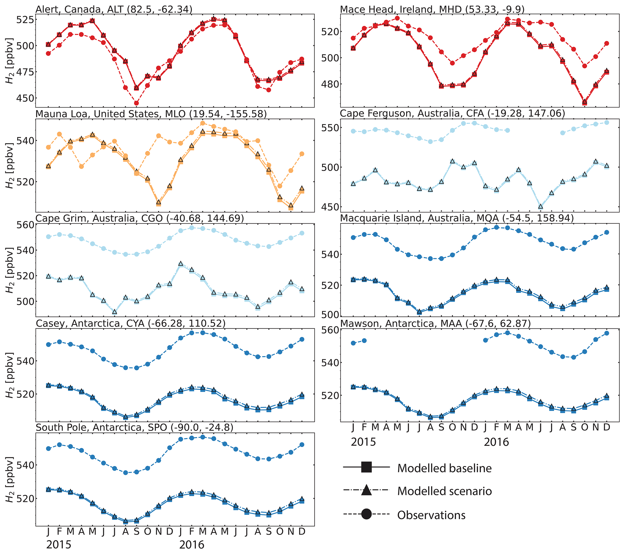
Figure 5 Seasonal cycle comparisons of H₂ dry mixing ratios at the eight sites from the CSIRO and AGAGE flask measurements for 2015 and 2016 (Krummel et al., 2021a, b, c, d, e, f, g, h; Wang et al., 2021). The dashed line with circle markers shows the observed values, the continuous line with square markers shows the modeled values from the GEOS-Chem baseline simulation and the dash-dotted line with triangle markers shows the modeled values from the GEOS-Chem aldehyde photolysis scenario. The colors are the same as in Fig. 3. For a comparison of the modeled and observed CO at the same sites see Fig. S9.

Photolytic H₂ production from aldehydes was added to the existing standard chemistry mechanism using the kinetic preprocessor (KPP) embedded within GEOS-Chem. We assigned the 1 % quantum yield found by Harrison et al. (2019) for acetaldehyde to the selected aldehydes tested in GEOS-Chem, analogously to what was done for the box modeling (Sect. 2.1). The 1 % from acetaldehyde was taken as the reference quantum yield to test given that measurements for the rest of the aldehydes are not available, but the energy barriers for the production of H₂ from aldehyde photolysis indicate that the dissociation channels are accessible (Rowell et al., 2022). For acetaldehyde, glycolaldehyde, HPALD and RCHO, a branching ratio on the existing photolysis channels was added to account for the primary production of H₂ in addition to the existing photolysis products. For methacrolein and methylglyoxal, additional steps had to be taken as the current GEOS-Chem implementation of Fast-JX for methacrolein and methylglyoxal embeds the quantum yields in the provided cross sections. For these species, new photolysis channels were created that separated the cross sections from the quantum yield. The cross sections for the two species were retrieved from Sander et al. (2020) and processed using the Fast-J v7.3c model, which covers 18 wavelength bins from 177 to 850 nm (Prather, 2015). The resulting binned cross sections and 1 % quantum yield were then configured back into the customized version of Fast-JX v7.0 used in GEOS-Chem (Eastham et al., 2014). Beyond these changes to the photochemistry, all other sources and sinks were identical to those used in the baseline. We ran this modified version of the simulation with the new photochemistry from June 2014 to December 2016, again using the first 6 months as spin-up. This simulation will hereafter be referred to as the aldehyde photolysis scenario.

Figure 6 shows the percentage difference in total tropospheric H₂ chemical production between the aldehyde photolysis scenario and the baseline simulation. The increase in the chemical production of H₂ from the new photochemistry for aldehydes is widespread across the globe. Figure 6a shows that the increase in total column H₂ chemical production reached a maximum of ∼10 %, with the biggest changes taking place over the Amazon. Forested regions in the African tropics, Indonesia, Papua New Guinea and northeast Australia show increases that ranged from 2 % to 8 %. At the surface (Fig. S10a), the increase in H₂ chemical production was up to 14 % with the same spatial distribution as seen in Fig. 6a for the troposphere as a whole. In the vertical profile (Fig. 6b, c), the increases in H₂ chemical production extended to 700 hPa over the tropics. This increase well above the surface layer may be a result of the strong vertical transport in this region, with rapid transport of aldehydes from the surface to the mid-troposphere followed by their photolysis to yield H₂.

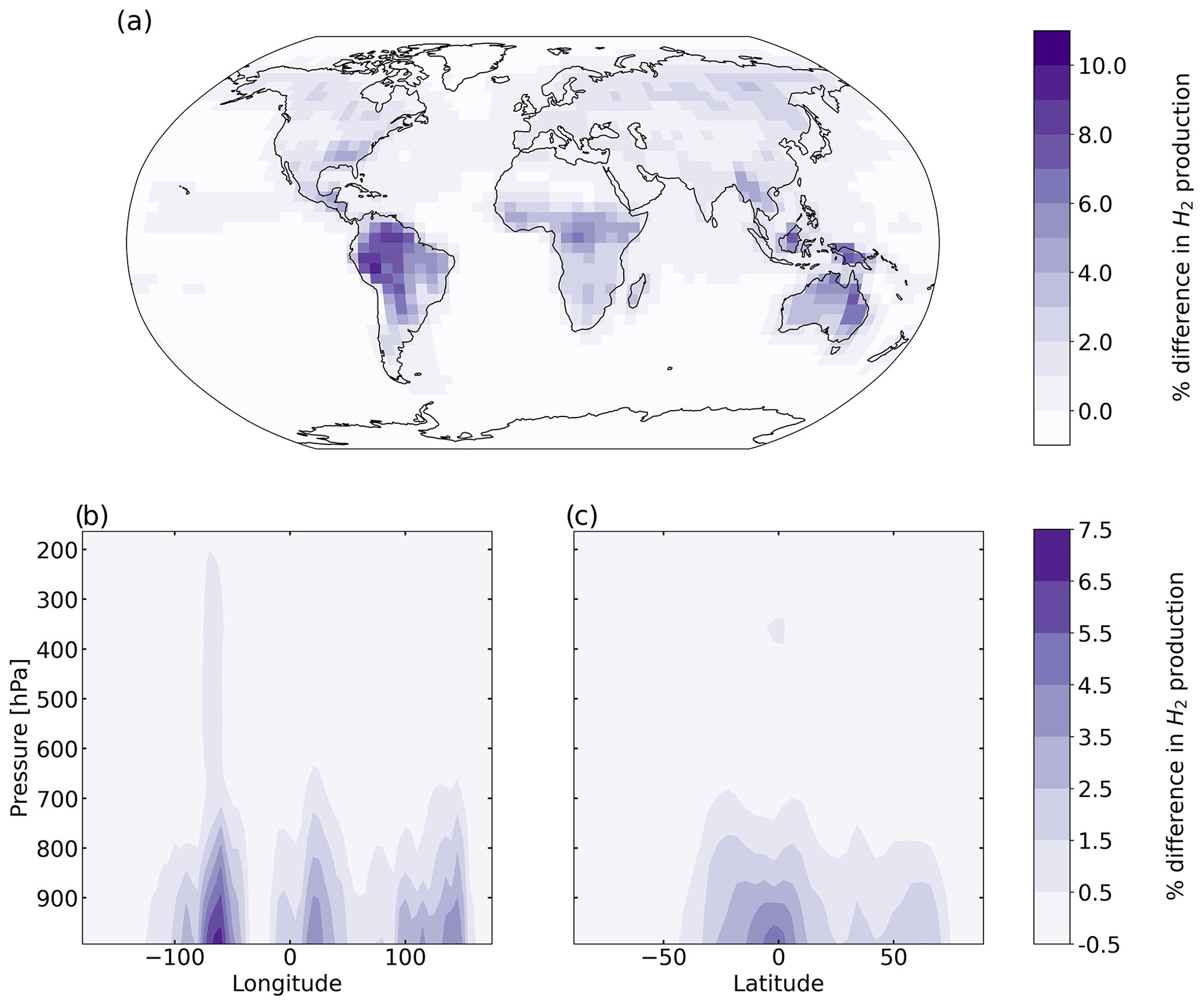
Figure 6 Percentage difference in tropospheric H₂ chemical production between the aldehyde photolysis scenario (with 1 % H₂ quantum yield) and the baseline simulation, averaged over 2015 and 2016. Results are shown (a) spatially (summed over the tropospheric column), (b) as a function of altitude and longitude (summed over latitudes), and (c) as a function of altitude and latitude (summed over longitudes).

The strongest response to the new aldehyde photochemistry is seen in regions with dense vegetation cover characterized by high isoprene emissions. The most relevant aldehydes for the formation of H₂ over densely vegetated areas are thus those related to the oxidation of isoprene and of its primary products, methacrolein and methyl vinyl ketone. Of particular importance here are methylglyoxal and glycolaldehyde, products from the OH-initiated oxidation of both methacrolein and methyl vinyl ketone, which account for ∼79 % and ∼49 %, respectively, of the global sources of these aldehydes (Fu et al., 2008; Wennberg et al., 2018).

We conducted additional model sensitivity simulations to compare the H₂ production from each of the new aldehyde sources (e.g., excluding formaldehyde and glyoxal). From these sensitivity simulations, we find that methylglyoxal contributes approximately 91 % to the enhanced tropospheric H₂ chemical production from these additional aldehydes (Fig. S11a) while glycolaldehyde, methacrolein and the other non-isoprene-related aldehydes (acetaldehyde, HPALD and RCHO) collectively account for the remaining 9 % (Fig. S11b). These results imply that the most relevant aldehyde to include in global model simulations for the direct photochemical formation of H₂ is methylglyoxal. We note that the estimated methylglyoxal mixing ratios in our simulations (Fig. S12) are comparable to those modeled and reported by Fu et al. (2008). Fu et al. (2008) compared their modeled methylglyoxal estimates against available observations finding no systematic bias at land sites. Although Fu et al. (2008) used few northern midlatitude locations to perform their comparison, the similarity between our methylglyoxal mixing ratios and the ones by Fu et al. (2008) gives us confidence in our modeled methylglyoxal and subsequent generation of H₂ from its photolysis.

Despite the substantial increase in H₂ chemical production associated with the new aldehyde photochemistry, the change in the tropospheric H₂ mixing ratios is very small, with a maximum change of 0.3 % over South America as shown in Fig. 7a. This equates to a change at the surface over South America of ∼0.5 % (see Fig. S13a). As seen previously for the chemical production, the biggest changes occur over the tropics. The influence of long-range transport (facilitated by the ∼2-year H₂ lifetime) can be seen in the figure, with an increase of up to 0.2 % in the H₂ mixing ratios over the oceans. Figure 7b and c also show the injection of H₂ to higher levels in the troposphere, particularly in the tropics where the increase extends to 500 hPa, but as seen in the figure, the enhancement in the mixing ratios does not exceed ∼0.2 %. At higher latitudes, the change is almost imperceptible, as expected by the lack of precursor aldehydes at those latitudes.

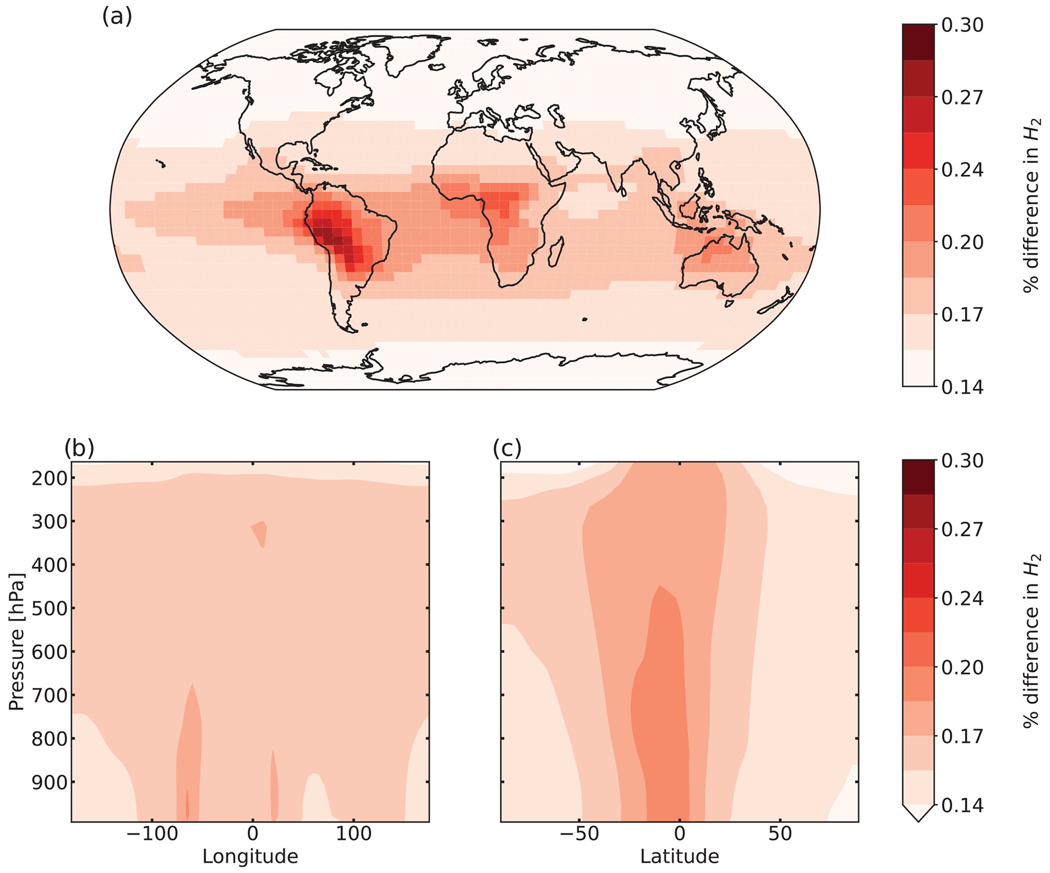
Figure 7 Same as Fig. 6 but for average H₂ mixing ratios.

Figure 8 displays the absolute differences between the aldehyde photolysis scenario and the baseline simulation for chemical production (a), chemical loss (b) and soil uptake (c), all at the surface layer. The enhanced H₂ chemical production in the tropics discussed previously (Fig. 8a) is compensated for by increased soil uptake of H₂ (Fig. 8c), with both showing maximum values over the Amazon. Elsewhere the situation is much the same: the enhanced H₂ produced from aldehyde photolysis is largely deposited in the same locations, making the atmospheric enhancement of H₂ from aldehyde photolysis small. This implies that the increases in production had a tendency to occur in places and times where the loss rates are stronger than the global average. Although the effect is smaller than seen for the soil sink, the chemical loss of H₂ from reaction with OH (Fig. 8b) also increases as expected in response to the enhanced production, further contributing to the balance between additional H₂ production and loss in the aldehyde photolysis scenario.

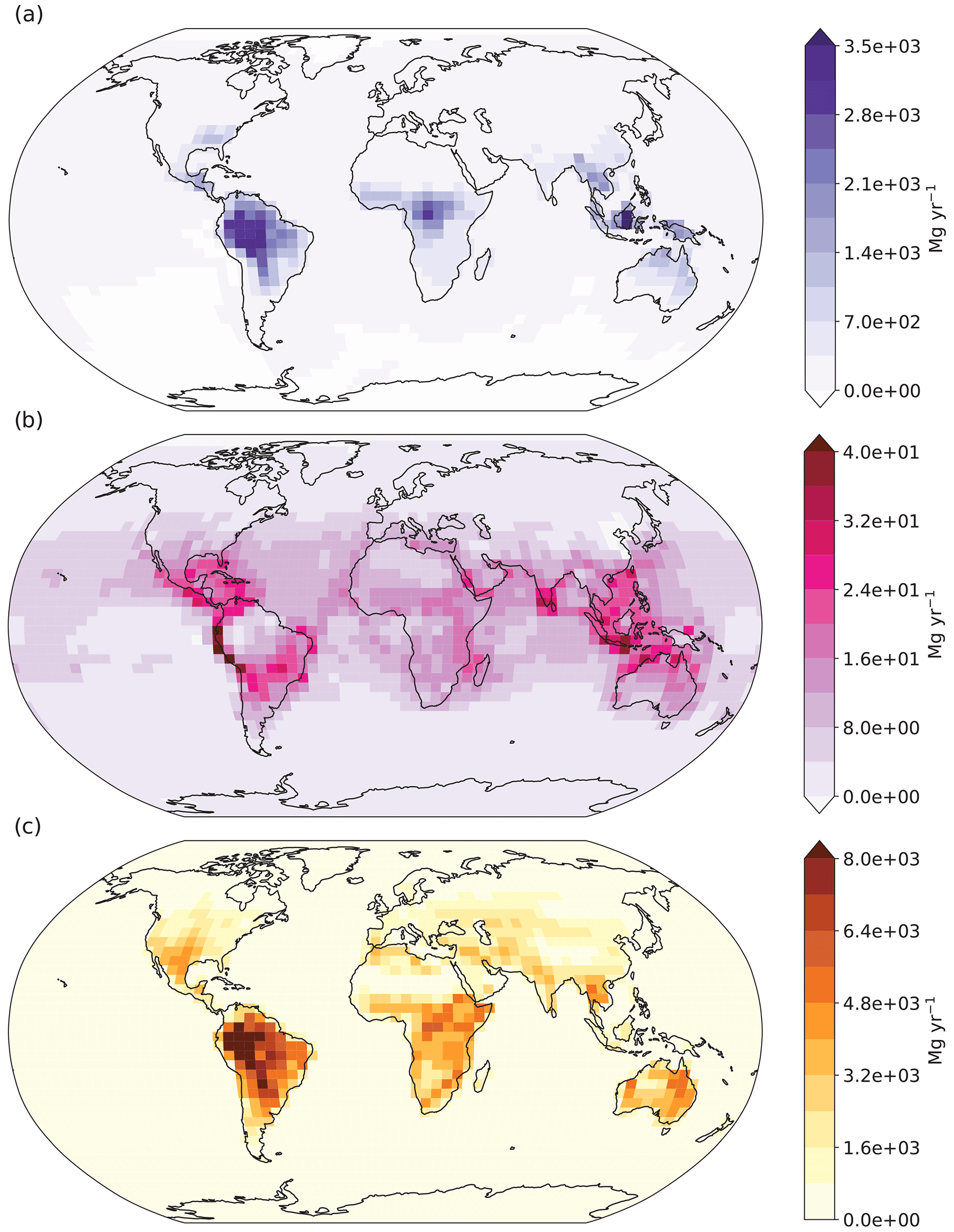
Figure 8 Absolute differences at the modeled surface layer between the aldehyde photolysis scenario (with 1 % quantum yield of H₂ from aldehydes) and the baseline simulation for (a) H₂ chemical production, (b) H₂ chemical loss, and (c) H₂ uptake by soil. Units for all plots are megagrams per year (Mg yr⁻¹). Note the differences in scale between the plots.

The tropospheric budget from the aldehyde photolysis scenario is shown alongside the budget from the baseline simulation in Table 2. Overall, the new photochemistry led to an increase in H₂ sources, sinks and tropospheric burden compared to the baseline simulation but all remained within the ranges reported by previous studies (Table 2). Summed over the global troposphere, the total increase in tropospheric H₂ chemical production from inclusion of direct H₂ production from newly discovered aldehyde photolysis was only 0.98 % for 2015 and 0.96 % for 2016. Given the small changes in H₂ mixing ratios described above, there were no significant changes in model performance relative to observations at measurement sites. The low model bias observed in the Southern Hemisphere did not improve, which allows us to conclude that missing chemical sources are not likely to resolve the remaining uncertainties and biases in the modeled H₂ seen in the baseline simulation.

4 Summary and conclusions

Recent laboratory findings by Harrison et al. (2019) identified a previously unknown H₂ channel for acetaldehyde yielding H₂ at a 1 % quantum yield. This finding by Harrison et al. (2019) was complemented by aldehyde ground-state calculations that show that the direct H₂ channel is also possible for other aldehydes (Rowell et al., 2022). Here, we assessed the impact of the recently determined direct generation of H₂ from aldehyde photolysis using two photochemical models: the AtChem v1.2 box model implementing the Master Chemical Mechanism MCM v3.3.1 and a modified version of the GEOS-Chem v12.5.0 3-D chemical transport model.

We configured the box model at three sites (London, Cabo Verde and Borneo) to explore the production of H₂ under distinctive atmospheric conditions and constrained each box model simulation with measurements. The standard MCMv3.3.1 considers 18 aldehydes and their corresponding reactions, with formaldehyde and glyoxal already including a H₂ channel. We evaluated the generation of H₂ from the remaining 16 aldehydes in MCM by comparing a baseline simulation against four sensitivity scenarios each using different H₂ quantum yields (1 %, 2 %, 5 % and 10 %). The selected quantum yields for the sensitivity analysis were chosen based on experiments by Kharazmi (2018) that showed that methylpropanal has an 8 % quantum yield for the H₂ channel. Our box model results allowed us to identify the aldehydes that are more likely to contribute to the H₂ production.

Excluding the contributions from formaldehyde and glyoxal, which remain the biggest photochemical H₂ sources, in an urban atmosphere, aliphatic aldehydes such as acetaldehyde and propanal contributed over 80 % of the simulated photochemical generation of H₂ from aldehydes. Unsaturated olefinic aldehydes and vegetation-related species like methylglyoxal, methacrolein and acrolein provided a collective contribution of less than 10 %. The remaining minor contributions came from glycolaldehyde. In a marine atmosphere, results were similar, with acetaldehyde and propanal contributing to 90 % of the H₂. In an atmosphere over a tropical rainforest, the oxidation products of vegetation-emitted species (i.e., methylglyoxal, glycolaldehyde, methacrolein and acrolein) contributed to 81 % of the H₂ produced. Based on the contribution at each modeled site, out of the 16 aldehydes tested with MCM, 6 were identified as the most relevant for H₂ production: acetaldehyde, propanal, glycolaldehyde, methylglyoxal, methacrolein and acrolein. Based on this finding from the box modeling, the global impacts of H₂ production from five of these aldehydes (excluding acrolein) were further investigated by using global atmospheric chemical transport modeling.

We then developed a global GEOS-Chem simulation of H₂ by modifying the v12.5.0 code to simulate H₂ as an active species with tropospheric sources including direct emissions from anthropogenic combustion and biomass burning sources and photochemical production from formaldehyde and glyoxal, along with sinks from reaction with OH and soil uptake parameterized as a dry deposition flux. We simulated 2015–2016 (preceded by a 6-month spin-up) and compared the results against available measurements (Krummel et al., 2021b, c, d, e, f, g, h, a, i; Wang et al., 2021). The model performance analysis showed our new GEOS-Chem baseline H₂ simulation is able to reproduce the seasonal cycle of H₂ at the different measured sites. Model performance was better in the Northern Hemisphere than in the Southern Hemisphere, where a persistent low bias was present. An overestimation of sinks and/or missing H₂ sources (particularly from the ocean) may explain the observed low model bias and should be investigated in future work. In the Northern Hemisphere, high estimates in East Asia seen for both H₂ and CO are likely due to overestimates in anthropogenic emissions. Our simulated tropospheric budget of H₂ indicated a global burden of ∼158 Tg yr⁻¹ and a lifetime of ∼2 years, consistent with previous studies (see Table 2). Overall, the model performance was deemed satisfactory for use as a baseline simulation to compare to a modeled scenario with new H₂ production from aldehyde photolysis.

Six aldehydes were tested in GEOS-Chem, each with a 1 % quantum yield channel for H₂: acetaldehyde, propanal (part of the lumped RCHO species), glycolaldehyde, methylglyoxal, methacrolein and hydroperoxyaldehyde (HPALD). We ran the model for the same 2 years as the baseline simulation (2015–2016), again with 6-month spin-up, and compared the results against the baseline. We calculated a maximum increase in the tropospheric H₂ chemical production over tropical regions of ∼10 % as a result of the new aldehyde photochemistry. The spatial distribution of the newly produced H₂ correlated well with the distribution of aldehydes associated with isoprene oxidation: glycolaldehyde, methylglyoxal and methacrolein. Using additional sensitivity studies, we found that over 90 % of the new chemical production could be attributed to methylglyoxal.

The ∼10 % increase in the chemical production of H₂ yielded an additional $\sim \mathrm{3.6}\times {\mathrm{10}}^{-\mathrm{3}}$ Mg yr⁻¹, an amount that was ultimately balanced by an increase in the chemical loss and soil uptake of H₂. The result of compensating sources and sinks in the aldehyde photolysis scenario was a maximum effective change of only 0.3 % in the tropospheric mixing ratios, which was seen over South America. The minimum change in the tropospheric H₂ mixing ratios associated with the new photochemistry was 0.14 %, found over the poles where aldehyde precursors are negligible. The additional H₂ source from aldehyde photolysis therefore did not improve the low model bias in the Southern Hemisphere seen in the baseline simulation. This means that other processes besides the photolytic loss of aldehydes are more likely responsible for the lingering discrepancies between model and measurements. These include both the emissions (natural and anthropogenic) and the soil uptake processes. Future work should focus in particular on improvements to anthropogenic emissions in areas with high bias, such as China and Korea, and ocean emissions in the Southern Hemisphere.

The implementation of the new aldehyde photochemistry in the two models yields consistent results, showing that the biggest changes in the chemical production of H₂ will occur for areas with a sizable source of biogenic VOCs that can serve as precursors for the most relevant aldehydes identified in this work. Both models point to methylglyoxal as a potentially relevant photochemical source of H₂. The box model highlights an additional possible contribution from glycolaldehyde. The fact that methylglyoxal and glycolaldehyde make significant contributions to modeled H₂ production in our simulations is significant. While we did not distinguish here between different types of aldehydes, Rowell et al. (2022) explain that the aldehydes that most likely yield H₂ in the troposphere are those with a triple fragmentation (TF) channel with energies below 350 kJ mol⁻¹. Sufficiently low TF energy barriers have been calculated for both methylglyoxal (330 kJ mol⁻¹) and glycolaldehyde (229 kJ mol⁻¹) (Rowell et al., 2022). Glycolaldehyde has the lowest energy barrier for the TF channels of any of the aldehydes calculated by Rowell et al. (2022). The glycolaldehyde TF energy barrier is even lower than that of propanal (295 kJ mol⁻¹), which has been shown to have a H₂ quantum yield of ∼8 % (Kharazmi, 2018). Thus, both methylglyoxal and glycolaldehyde are the aldehydes that are theoretically most likely to have a H₂ channel based on the calculations from Rowell et al. (2022) and (for glycolaldehyde at least) may have a H₂ quantum yield greater than the 1 % tested in our simulations. The experimental determination of H₂ quantum yields from a TF channel for methylglyoxal and glycolaldehyde should therefore be prioritized. Further, our estimates for the contribution of methylglyoxal and glycolaldehyde to the photochemical generation of H₂ may well represent a lower limit of the true contribution.

Finally, our new GEOS-Chem H₂ simulation capability, including the new photochemistry for the direct generation of H₂ from aldehydes, provides a useful tool for other studies of H₂. This model can serve as a framework for interpreting historical H₂ distributions and variability, improving process-level understanding of H₂ cycling, and testing future H₂ emission scenarios. The latter will become increasingly important as plans to migrate to the H₂ economy begin to materialize.