The ozone–climate penalty over South America and Africa by 2100

Climate change has the potential to increase surface ozone (O₃) concentrations, known as the “ozone–climate penalty”, through changes to atmospheric chemistry, transport and dry deposition. In the tropics, the response of surface O₃ to changing climate is relatively understudied but has important consequences for air pollution and human and ecosystem health. In this study, we evaluate the change in surface O₃ due to climate change over South America and Africa using three state-of-the-art Earth system models that follow the Shared Socioeconomic Pathway 3-7.0 emission scenario from CMIP6. In order to quantify changes due to climate change alone, we evaluate the difference between simulations including climate change and simulations with a fixed present-day climate. We find that by 2100, models predict an ozone–climate penalty in areas where O₃ is already predicted to be high due to the impacts of precursor emissions, namely urban and biomass burning areas, although on average, models predict a decrease in surface O₃ due to climate change. We identify a small but robust positive trend in annual mean surface O₃ over polluted areas. Additionally, during biomass burning seasons, seasonal mean O₃ concentrations increase by 15 ppb (model range 12 to 18 ppb) in areas with substantial biomass burning such as the arc of deforestation in the Amazon. The ozone–climate penalty in polluted areas is shown to be driven by an increased rate of O₃ chemical production, which is strongly influenced by NO_x concentrations and is therefore specific to the emission pathway chosen. Multiple linear regression finds the change in NO_x concentration to be a strong predictor of the change in O₃ production, whereas increased isoprene emission rate is positively correlated with increased O₃ destruction, suggesting NO_x-limited conditions over the majority of tropical Africa and South America. However, models disagree on the role of climate change in remote, low-NO_x regions, partly because of significant differences in NO_x concentrations produced by each model. We also find that the magnitude and location of the ozone–climate penalty in the Congo Basin has greater inter-model variation than that in the Amazon, so further model development and validation are needed to constrain the response in central Africa. We conclude that if the climate were to change according to the emission scenario used here, models predict that forested areas in biomass burning locations and urban populations will be at increasing risk of high O₃ exposure, irrespective of any direct impacts on O₃ via the prescribed emission scenario.

1 Introduction

Climate change threatens to bring new pressures to the tropical forests, grasslands and agricultural lands of Africa and South America. As a result of shifts in emissions, atmospheric chemistry and meteorology, as well as changes in vegetation behaviour such as transpiration rate, surface O₃ concentrations are likely to change (e.g. Turnock et al., 2019; Griffiths et al., 2021; Zanis et al., 2022), which may impair or benefit human and vegetation health (Agathokleous et al., 2019; Emberson, 2020) depending on the direction of change. O₃ is a highly oxidising compound, formed in the atmosphere through reaction of volatile organic compounds (VOCs) or carbon monoxide (CO) with hydroxyl radicals (OH) and nitrate radicals (NO₃) in the presence of nitrogen oxides (NO_x). However, it can also be removed from the atmosphere through reactions with many of the same chemical species (NO_x, VOC, OH) depending on their relative concentrations. In addition to chemical pathways, O₃ can be removed from the lower atmosphere by dry deposition, which includes stomatal uptake by plants (Silva and Heald, 2018). Stomatal uptake of O₃ and subsequent ozone plant damage can lead to reduced carbon drawdown from the atmosphere (Sitch et al., 2007; Yue and Unger, 2018; Franz and Zaehle, 2021) and changes to biosphere–climate interactions (Sadiq et al., 2017). Sitch et al. (2007) showed that the tropics may be especially sensitive to high O₃ concentrations and therefore susceptible to large productivity losses if surface O₃ were to increase. Additionally, O₃ is a near-term climate forcer with impacts on the radiative balance leading to a positive radiative forcing of climate through absorption of longwave radiation (Myhre et al., 2017). As the tropical forests are vital as sinks for atmospheric CO₂ and tropical ecosystems play a vital role in regional and global climate (Lewis, 2006; Bonan, 2008), an understanding of the impact of climate change on surface O₃ concentrations in the tropics is critical.

Whilst there have been no studies specifically assessing changes in surface O₃ due to climate change in the tropics, global studies have suggested that chemical and biological changes in temperature-dependent chemistry, natural emissions of precursors and land surface properties; as well as dynamical changes including circulation changes and transport from the stratosphere may lead to an “ozone–climate penalty” over some continental areas (Jacob and Winner, 2009; Doherty et al., 2013; Zanis et al., 2022). The ozone–climate penalty is defined as an increase in surface O₃ concentrations due to climate change alone. It is influenced by many complex chemical and biological processes, which are not all well-understood or represented in current climate models, although there has been substantial recent research to reduce uncertainty in temperature-sensitive chemistry, meteorology and land–atmosphere feedbacks (Oswald et al., 2015; Coates et al., 2016; Sadiq et al., 2017; Romer et al., 2018; Archibald et al., 2020b). There has been relatively little research focusing on O₃ in tropical environments. Unlike the more commonly studied extra-tropical Northern Hemisphere, the tropics and subtropics have relatively low (natural) NO_x emissions and high biogenic VOC emissions, high actinic flux, and strong atmospheric convection (Bond et al., 2002; Pugh et al., 2010; Paulot et al., 2012). This paper focuses on South America and Africa. We exclude equatorial Asia because the atmospheric chemistry in this region is more uncertain due to difficulties in detecting and accounting for peat fire emissions (Prosperi et al., 2020). Equatorial Asia also has a greater marine influence with most model grid boxes containing ocean as well as land, so they may follow a different chemical regime.

Many areas in Africa and South America are considered remote (defined in this paper by low emissions of NO_x), although increasing anthropogenic activity such as urbanisation and biomass burning causes moderate NO_x emissions in some regions (e.g. Kuhn et al., 2010; Pacifico et al., 2015; Shi et al., 2020). The sensitivity of O₃ production to NO_x depends on the relative concentrations of NO_x and VOCs. Isoprene is the most abundant biogenic VOC in remote Africa and South America and must be oxidised in the atmosphere before it can form O₃ (Liu et al., 2016). NO_x is produced from both natural and anthropogenic sources including soils, lightning, transport and biomass burning. In NO_x-limited regimes where O₃ production is proportional to NO_x concentrations, increasing VOCs or OH can also act to reduce O₃ concentrations through oxidation and formation of organic peroxides (Pacifico et al., 2012). In this NO_x-limited case, increasing NO_x will lead to greater O₃ formation. Conversely, in VOC-limited regions with sufficient NO_x present, increasing NO_x concentrations may reduce O₃ concentrations by removal of the key O₃-forming radicals OH (reaction: $\mathrm{OH}+{\mathrm{NO}}_{\mathrm{2}}\to {\mathrm{HNO}}_{\mathrm{3}}$).

Earlier studies have found that South America and Africa are generally NO_x-limited (Ziemke et al., 2009; Bela et al., 2015) and that increases in NO_x concentration associated with climate change will be a key driver of O₃ increases over South America and Africa. Doherty et al. (2013) attribute the NO_x increase predominantly to enhanced decomposition of the NO_x reservoir species, peroxyacetyl nitrate (PAN). A fraction of emitted NO_x is locked up as PAN, which decomposes back into NO_x in warmer temperatures, sometimes after having travelled long distances from the NO_x source. As PAN is unstable at high temperatures, climate change will result in a smaller fraction of NO_x being stored as PAN in NO_x source regions and may also decrease the amount of NO_x that is transported into remote regions (Schultz et al., 1999; Finney et al., 2018). Lightning NO_x is known to contribute to O₃ formation; however studies project both increases and decreases in future lightning frequency (Clark et al., 2017; Finney et al., 2018) leading to low confidence in how O₃ will be affected by climate-driven changes in lightning (Fu and Tian, 2019; Murray, 2016).

The role of isoprene in the ozone–climate penalty is debated as there is uncertainty about how isoprene emissions will change in the future in response to temperature, CO₂ and land-use change (Fu and Liao, 2016; Fu and Tian, 2019) and how to best represent isoprene chemistry in climate models (Weber et al., 2021). Biogenic isoprene emissions increase strongly with temperature and vegetation stress (e.g. Guenther et al., 1993; Niinemets et al., 1999; Unger et al., 2013; Morfopoulos et al., 2021), but very high temperatures or moisture stress may cause “die-back” of vegetated areas, which would decrease isoprene emissions overall (Sanderson et al., 2003; Cox et al., 2004; Malhi et al., 2009). On the other hand, elevated CO₂ concentrations directly inhibit isoprene emission but can indirectly increase emission if this CO₂ fertilisation effect results in increased plant productivity (Pacifico et al., 2011; Squire et al., 2014; Hantson et al., 2017). Isoprene, NO_x and OH concentrations are influenced by isoprene chemistry. Formation of isoprene nitrates partially recycles NO_x, and oxidation of isoprene partially recycles HO_x (Bates and Jacob, 2019). The difference between models in their calculation of the yields and recycling rates of these species is likely to affect O₃ concentrations.

Besides chemical processes, dry deposition of O₃ to vegetation is a major O₃ sink, accounting for 20 % of O₃ removal (Wedow et al., 2021). Most O₃ deposition occurs via plant stomata, which respond to changes in the climate. (Silva and Heald, 2018; Clifton et al., 2020). Increased CO₂, temperature and vapour pressure deficit (VPD) will decrease stomatal conductance and therefore decrease O₃ deposition rate. This could lead to increased concentrations of O₃ in the atmosphere, although it would have a protective effect for plants (Emberson et al., 2013; Lin et al., 2020).

Studies agree that over the ocean, average surface O₃ concentrations will decrease under the influence of climate change (Zeng et al., 2008; Doherty et al., 2013; Zanis et al., 2022). The warmer air can hold more water vapour, a major species contributing to O₃ loss (reaction: $\mathrm{O}\left(\mathrm{1}\mathrm{D}\right)+{\mathrm{H}}_{\mathrm{2}}\mathrm{O}\to \mathrm{2}\mathrm{OH}$ leading to O₃ loss via ${\mathrm{OH}}_{\mathrm{2}}+{\mathrm{O}}_{\mathrm{3}}\to \mathrm{OH}+\mathrm{2}{\mathrm{O}}_{\mathrm{2}}$). There may also be O₃ reductions in remote regions over land due to this process, although natural emissions can change the atmospheric chemistry over the continents. Other factors contributing to the O₃ concentration over the continents are numerous and complex, including changes to oxidising capacity, stratospheric transport and land use (Archibald et al., 2010; Squire et al., 2015).

This paper quantifies the effect of climate change on surface O₃ concentrations in the future and aims to understand its uncertainty and the relative contributions of the underlying processes. We focus on areas with robust O₃ changes to identify areas in South America and Africa at greatest risk by 2100. Section 1 has introduced the key chemical species involved in O₃ chemistry and the most important changes that may result from climate change. In Sect. 2, we provide the model details, data used for evaluation and description of analysis of model output. Section 3 evaluates model predictions of surface O₃ in the present day, evaluates model predictions for surface O₃ changes in 2100 and examines the importance of chemical and deposition changes in controlling the ozone–climate penalty in models. Finally, Sect. 4 discusses the key trends predicted by the models, limitations of the study and crucial uncertainties in the models.

2 Methods

We analyse surface O₃ for simulations that follow a medium–high-emission pathway created for CMIP6 (Pascoe et al., 2020). The simulations were carried out as part of an ensemble of Earth system model experiments designed to quantify the climate and air quality impacts of aerosols and trace gases in climate models (Collins et al., 2017), named Aerosol-Chemistry Model Intercomparison Project (AerChemMIP). For this study three Earth system models were used: UKESM1-0-LL (abbreviated UKESM1), GISS-E2-1-G (abbreviated GISS), MRI-ESM2-0 (abbreviated MRI). These were selected because of their detailed tropospheric chemistry schemes and availability of output for O₃ and O₃ precursor concentrations on the Earth System Grid Federation (ESGF).

The simulations follow the Shared Socioeconomic Pathway 3-7.0 (SSP3-7.0) emission scenario, a scenario assuming low international cooperation to protect the environment. This includes high emissions of non-methane near-term climate forcers and substantial land-use change (O'Neill et al., 2016; Gidden et al., 2019). The prescribed emissions include anthropogenic and biomass burning emissions of NO, CO₂ and CO (Rao et al., 2017; Riahi et al., 2017) and the future pathway for CH₄ is calculated as an atmospheric concentration (Meinshausen et al., 2020). Emissions due to growing populations and poor international cooperation result in significant temperature increases by 2100 (Turnock et al., 2019) and societies that are highly vulnerable to climate change. This emission pathway was chosen in order to understand changes in end-of-century O₃ concentration if there is no international cooperation to reduce precursor emissions.

2.1 Model descriptions

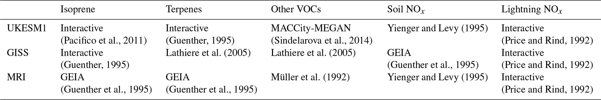
A comparison among models of natural emissions that may respond to the climate are shown below (Table 1). Where emissions are prescribed, the source is provided. Emissions that are interactive will respond to climate change. Further details on each of the Earth system models, including descriptions of the interactive emissions schemes and the tropospheric chemistry schemes, are provided below.

Table 1 Sources of natural emissions of ozone precursors. Where emissions are prescribed, the source is provided. Interactive emissions respond to climate change.

2.1.1 UKESM1-0-LL (abbreviated UKESM1)

UKESM1-0-LL is a combination of HadGEM3 (Williams et al., 2018) with additional land and atmospheric chemistry components (Sellar et al., 2019). The UK Chemistry and Aerosol scheme (UKCA) contains stratospheric and tropospheric chemistry (Archibald et al., 2020a) combined with the GLOMAP-mode aerosol microphysics scheme (Mulcahy et al., 2018; Mulcahy et al., 2020).

Interactive emissions include isoprene, monoterpenes and lightning NO_x. Isoprene and monoterpene emissions respond to light and temperature (Archibald et al., 2020a; Mulcahy et al., 2018). Isoprene emissions are calculated from vegetation productivity and increase in response to light and temperature (with an optimum at 40 ^∘C). Emissions of isoprene are inhibited by CO₂ following the emission model of Pacifico et al. (2011). Lightning NO_x is calculated using the parameterisation of Price and Rind (1992), which calculates a lightning flash density based on cloud-top height. Nitrogen oxide molecules produced per flash are 7.5×10²⁶ for cloud-to-ground flashes and 2.25×10²⁶ for cloud-to-cloud flashes. Secondary organic aerosols (SOAs) are calculated as a fixed yield of 26 % from gas-phase oxidation reactions involving monoterpene sources. Soil NO_x is prescribed as an annual flux of 12 Tg, according to Yienger and Levy (1995) and other biogenic emissions are prescribed as monthly mean climatologies based on the years 2001–2010 (Guenther et al., 2012).

The terrestrial biogeochemistry is provided by JULES (Wiltshire et al., 2020, 2021). Stomatal conductance in JULES is similar to the Ball–Berry–Leuning model (Leuning, 1995) and responds to the ratio of internal to external CO₂ concentrations and leaf humidity deficit (Jacobs, 1994).

The model has a horizontal resolution of 1.25^∘ latitude by 1.875^∘ longitude with 85 vertical levels in a hybrid height coordinate.

2.1.2 MRI-ESM2-0 (abbreviated MRI)

MRI-ESM2-0 (Yukimoto et al., 2019; Kawai et al., 2019; Oshima et al., 2020) contains an atmospheric and land surface model (MRI-AGCM3.5), an ocean and sea-ice model (MRI.COMv4), an aerosol model (MASINGAR mk-2r4c), and an atmospheric chemistry model (MRI-CCM2.1). The chemistry model includes tropospheric, stratospheric and mesospheric chemistry with 90 chemical species and 259 chemical reactions (Deushi and Shibata, 2011).

Lightning NO_x is interactive and based on a lightning flash density parameterisation (Price and Rind, 1992). A cloud-to-ground flash produces 6.7×10²⁶ molecules per flash and a cloud-to-cloud flash produces 6.7×10²⁵ molecules per flash. Other natural emissions from land and ocean are prescribed as monthly climatologies, including isoprene and soil NO_x (Deushi and Shibata, 2011). For aerosol formation, 15 % of natural terpene emissions at the surface form SOAs, and SOAs have identical properties to POA.

Each component employs different horizontal resolutions, but the outputs used in this paper are from the chemistry component, which uses a horizontal resolution of 2.8125^∘ latitude by 2.8125^∘ longitude with 80 vertical levels in a hybrid sigma pressure coordinate.

2.1.3 GISS-E2-1-G (abbreviated GISS)

GISS-E2-1-G contains a coupled troposphere and stratosphere chemistry scheme using the G-PUCCINI chemistry mechanism (Shindell et al., 2013; Kelley et al., 2020) combined with the One-Moment Aerosol (OMA) scheme for aerosols (Bauer et al., 2020).

Lightning NO_x is interactive as described by Kelley et al. (2020). The NO yield is 1.75×10²⁶ molecules per flash. Soil NO_x is prescribed as a monthly mean from GEIA. Isoprene emissions are interactive and respond to light and temperature (Shindell et al., 2006) following the algorithm defined by Guenther et al. (1995). Monoterpenes are prescribed as monthly means from Lathiere et al. (2005) based on the year 1990. SOAs are calculated using the carbon bond mechanism 4 (CBM4) to describe the gas-phase tropospheric chemistry together with all main aerosol components. Isoprene (VOCs) contribute to the formation of SOA (Tsigaridis and Kanakidou, 2018).

GISS has a horizontal resolution of 2.00^∘ latitude by 2.25^∘ longitude with 40 vertical levels output on hybrid sigma pressure coordinate.

2.2 Data analysis methods

2.2.1 Model evaluation

In situ observations from 65 sites across South America and tropical Africa, covering key biomes and land-use types, are used for grid level model evaluation. Monthly mean O₃ concentrations from individual sites have been aggregated into seven regions by grouping together sites within latitude and longitude bounds (see Table S1 in the Supplement). To compare these to models, the coordinates of the in situ measurement sites are matched to the nearest model grid cell coordinates. To create an average seasonal cycle for each region, sites with the same nearest grid cell are averaged together to create a grid cell seasonal cycle. Then, grid cell seasonal cycles in the same region are averaged together. Monthly mean data from 1990 up to 2021 were used, although most sites only provide a few years of data. Data were excluded if there was an unequal distribution of data points over the monthly mean diel cycle.

To produce a model seasonal cycle, the monthly mean O₃ concentration was calculated using CMIP6 historical simulations for the period 1990–2014. This was done for each grid cell that contained an observation site. The standard deviation in monthly mean O₃ concentrations between the grid cells used was calculated for each region (i.e. it represents variation in O₃ geographically between the sites rather than inter-annual variation).

For model evaluation against Tropospheric Emission Spectrometer (TES) data from the Aura satellite, which retrieves O₃ in parts per billion over 67 pressure levels, we use O₃ concentrations at the lowest level available from TES (825 hPa). Monthly mean gridded outputs are used for the period 2004–2011, the period for which complete monthly mean data are available. As with the model output, satellite grid cell coordinates closest to the in situ site coordinates were selected. The monthly mean and standard deviation for each region was calculated, only using data from grid cells containing in situ sites.

2.2.2 CMIP6 model output

We isolate the effect of climate change on surface O₃ concentrations using the difference between two simulations which consider the same trajectory of anthropogenic emission changes but differ in climate. The simulations are global model runs driven with prescribed sea surface temperatures (SSTs) over the period 2015–2100. We use a simulation driven with changing SSTs from the coupled simulation ssp370 so that the climate changes in accordance with the emission changes; this simulation is named ssp370SST. We use a second simulation with prescribed SSTs and sea-ice concentrations taken from a present-day climatology (2005–2014) in historical simulations, named ssp370pdSST. Importantly, although anthropogenic emissions are identical in both simulations, ssp370pdSST does not include the resulting climate change.

To isolate the effect of climate change on tropospheric O₃, we subtract ssp370pdSST (present-day constant climate + future emissions) from ssp370SST (future climate + future emissions) following Zanis et al. (2022) and Szopa et al. (2021). Biomass burning and land-use change are considered anthropogenic and are prescribed for both models, but natural emissions are allowed to change depending on the model set-up. In this way, the background atmospheric composition is based on the future emission scenario used, since the response of atmospheric chemistry to climate change may depend on the background concentrations of precursors. In UKESM1, CO₂ is also fixed to present-day concentrations in ssp370pdSST so that the effect of climate change includes the effect of CO₂ inhibition.

Model output is taken as monthly means during the period 2090–2100 between 40^∘ S and 40^∘ N from experiments ssp370SST and ssp370pdSST. All variables used are outlined in Table S2 in the Supplement. The change due to climate change refers to subtracting ssp370pdSST from ssp370SST, where positive values are considered an O₃–climate penalty. When evaluating the change due to climate change regionally, this study distinguishes between “high-NO_x” and “remote” areas (Fig. 1). High-NO_x areas are defined as areas where the annual mean NO_x emissions are above the 95th percentile for the tropics and subtropics (40^∘ S–40^∘ N).

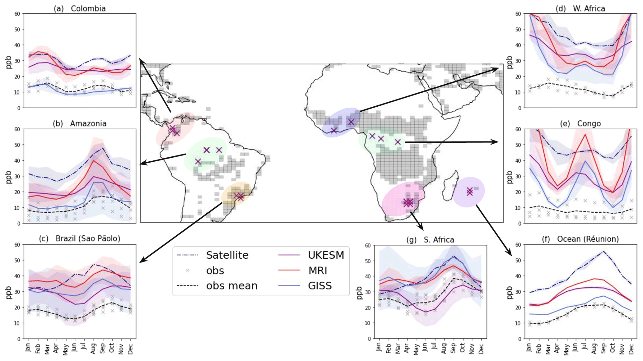
Figure 1 Panels (a–g) compare monthly mean O₃ (black dashed line) from site measurements averaged over seven regions to model predictions for the period 1990–2014 and satellite products from the TES satellite at 825 hPa (navy dash–dot line). Model means are shown for UKESM1 (purple solid line), GISS (blue solid line) and MRI (red solid line), and 2 standard deviations from the mean are shaded. Grey crosses indicate monthly mean O₃ measurements from individual sites and years. The central panel marks the locations where O₃ measurement sites are located (purple crosses) and how the sites have been grouped (coloured shading). Observations (a–c) and (f and g) use data from the Tropospheric O₃ Assessment Report (TOAR I; Schröder, 2021; Schultz et al., 2017), (d and e) from INDAAF data (2021) (http://indaaf.obs-mip.fr, last access: 9 October 2021) and (e) from CONGOFLUX in Yangambi, DR Congo. Grey grid cells cover areas where NO_x emissions are above the 95th percentile for the region 40^∘ S–40^∘ N in 2100 (prescribed by Rao et al., 2017; Riahi et al., 2017), indicative of biomass burning areas and cities. Unshaded areas are referred to as “remote” throughout.

O₃ concentrations are taken from the lowest model level (∼20 m above orography). Where multimodel means are shown, data have been re-gridded to the 2.8125^∘ by 2.8125^∘ grid used by MRI. We evaluate the ozone–climate penalty as a yearly average and seasonally. To identify seasonal patterns we aggregate the data by burning season. The western African burning season is defined as December–February, the southern African burning season is June and July, and the southern Amazon burning season is August–October.

To attribute the ozone–climate penalty to precursor variables, we also use NO_x, isoprene emission rate, OH and surface temperature variables. When presenting these variables, the ocean has been masked so that only land surface changes are presented. “Surface concentrations” shown in this study refer to chemical mixing ratios in the lowest model grid cells, and “background concentrations” refer to chemical mixing ratios in the absence of climate change (using data from ssp370pdSST).

To evaluate the O₃ budget, we also use O₃ chemical production, O₃ chemical loss and dry-deposition variables. O₃ chemical production is defined as O₃ produced from the reaction $\mathrm{NO}+{\mathrm{RO}}_{\mathrm{2}}/{\mathrm{HO}}_{\mathrm{2}}$, O₃ chemical loss is the sum of (i) O(1D)+H₂O, (ii) O₃+HO₂, (iii) O₃+OH and (iv) O₃+alkenes (e.g. isoprene). To compare these three variables on the same scale, we convert the units to Tg yr⁻¹ and sum production and loss over the lowest 1 km, the approximate boundary layer height. We choose 1 km to establish an approximate region that can contribute to surface O₃ concentrations.

In Sect. 3.4, we present a sensitivity study relating changes in NO_x concentration and isoprene emissions to changes in O₃ chemical production. We use monthly mean data in South America and Africa within 30^∘ S and 30^∘ N to calculate a monthly climatology for 2090–2100, masking the ocean and the non-vegetated region of Saharan Africa. To identify the limiting O₃ precursor in the tropics and subtropics, the percentage change in O₃ production rate (n>500) is modelled with an ordinary least squares linear regression using the percentage change in NO_x and isoprene as predictor variables (see Sect. S4 in the Supplement: the relationship between NO_x and O₃ production). To interpret the ability of the model we rely on the central limit theorem to assume that the normalised sum of the residuals can be approximated by a normal distribution. Unique months and grid cells are treated as separate data points. To present the results graphically, we highlight values using star markers if they are above a threshold of the 95th percentile for NO_x concentrations using the monthly climatology for each model individually, with aims to identify biomass burning areas and cities. The atmospheric chemistry in these areas may be different due to the elevated NO_x concentrations. Therefore, some grid cells will be above the 95th percentile for specific months only (biomass burning seasons).

3 Results

3.1 Evaluation of model skill for present-day surface O₃ concentrations

Results show that climate models are able to capture the observed seasonal cycle in most regions except for west Africa and DR Congo (Fig. 1). However, the models overpredict monthly mean surface O₃ concentrations by up to 50 ppb, with the largest bias present in remote forest locations such as the Congo area (Fig. 1e). GISS overall has the smallest positive bias out of all the models, and MRI has the largest. UKESM1 shows the smallest seasonal variation in O₃ concentration, which is often closer to the observed seasonal pattern.

Grey shading in Fig. 1 highlights the areas in South America and Africa with the highest NO_x emissions. The shaded areas represent areas with high biomass burning emissions and urban areas and are referred to as high-NO_x areas in this paper. In the southern Amazon (Fig. 1b), the biomass burning months are August and September, and both models and observations predict the highest O₃ concentrations in this season. However, the observed monthly mean O₃ concentrations range between 9 to 20 ppb, whereas models predict values up to 40 ppb, with GISS displaying the smallest positive bias. In Africa (Fig. 1d–f), the biomass burning months are December–February (west Africa) moving to June–July (southern Africa). Whilst models predict concentrations of up to 80 ppb in the Congo during these months due to transport of precursors from biomass burning, observations show substantially lower surface O₃ concentrations of less than 20 ppb at the remote locations sampled, although the highest O₃ concentrations occur during December–February (Adon et al., 2010, 2013; Ossohou et al., 2019). In fact, seasonal variation is low at the Congo sites, whereas models predict strong seasonal patterns (Fig. 1e). In months without substantial burning, GISS captures the low O₃ values well and UKESM1 and MRI overestimate them by 10 to 15 ppb.

The enhanced O₃ concentrations predicted by models in burning seasons over the Congo and west Africa are also captured in satellite retrievals at 825 hPa. Satellite O₃ concentrations in the DR Congo are 10 ppb higher in December–February compared to months without burning (Fig. 1e). At 825 hPa, these satellites capture O₃ concentrations above the altitude of in situ observation sites and the lowest model level. Model predictions for O₃ at 825 hPa are ∼10 ppb higher than the lowest model level and therefore compare well to satellite retrievals (Fig. S1 in the Supplement), especially in Amazonia (Fig. S1b) and west Africa (Fig. S1d).

Similar to biases over the remote continents, measurements from Réunion (Fig. 1f), which capture oceanic air masses, are overestimated by 5 ppb in GISS and by 12 ppb in UKESM1 and MRI, although the seasonal cycle is reproduced. On the other hand, over the urban sites in South Africa (Johannesburg), UKESM1 replicates the observed mean with moderate accuracy, whereas GISS and MRI overestimate it by 15 ppb (Fig. 1g).

3.2 Average changes to atmospheric composition over Africa and South America at the end of 2100

The overall change in O₃ concentration due to climate change over the African and South American land surface is shown in Fig. 2a for each model compared to the simulation with a fixed present-day climate. All models predict that on average O₃ concentrations will decrease due to climate change over the tropical land surface in this study. The magnitude of the predicted O₃ change for each model will depend on background concentrations of O₃ chemical precursors, their change due to climate change and individual model mechanistic details. There is significant diversity in background atmospheric composition between models (Fig. 2, blue marker) and the direction of change in surface NO_x and OH concentration due to climate change (Fig. 2b and c, arrows).

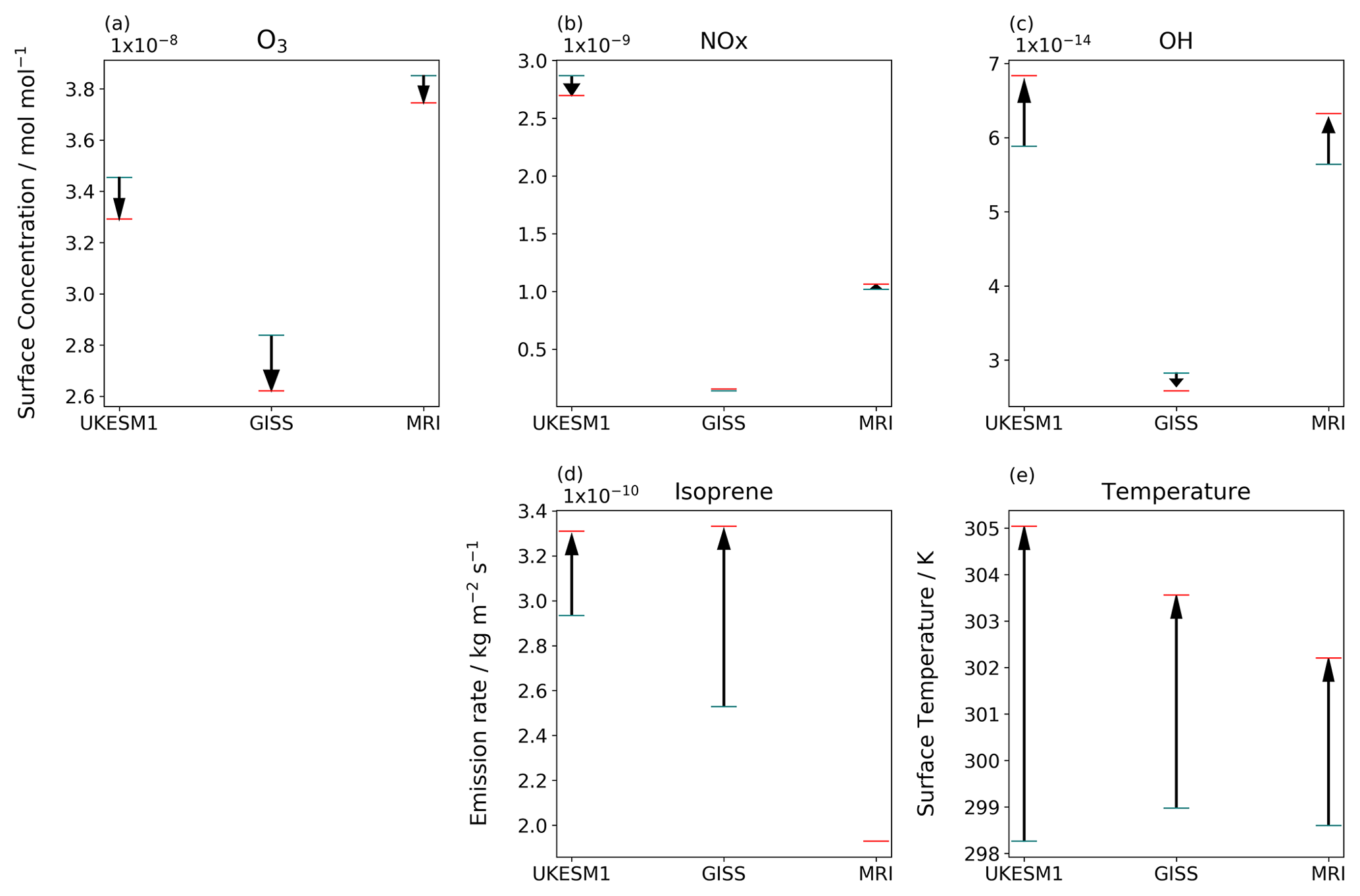
Figure 2 The change in surface concentration of (a) O₃, (b) NO_x and (c) OH, and the change in (d) isoprene emission rate and (e) surface temperature from experiment ssp370pdSST with no climate change (blue line) to experiment ssp370SST with climate change (red line) for the three climate models in this study. Variables have been averaged over the African and South American continents between 12^∘ N–30^∘ S for the period 2090–2100. The change due to climate change is significant at the 5 % level for all variables and models except isoprene in MRI (which is prescribed so does not change).

Different temperature sensitivities of the models (differing by up to 2.7 K) and different biogenic VOC schemes will contribute to the inter-model variation (Fig. S2 in the Supplement). UKESM1 has the greatest temperature sensitivity with a 6.5 K increase in temperature over the tropical land surface due to climate change (Fig. 2e). The temperature change due to climate change varies seasonally and regionally, which may affect concentration of O₃ precursors locally, with dry-season temperatures predicted to rise by 1–1.5 K more than wet-season temperatures (Fig. S3 in the Supplement).

The change in NO_x concentration between models is determined by the balance of changes in isoprene nitrate formation, OH concentrations, PAN decomposition and lightning in the models. A decrease in NO_x concentrations could be related to changes in OH concentration and precipitation (and thus NO_x removal via reaction ${\mathrm{NO}}_{\mathrm{2}}+\mathrm{OH}\to {\mathrm{HNO}}_{\mathrm{3}}$) and isoprene (and thus NO_x removal via isoprene nitrate formation), whereas NO_x concentration increases may be due to increased PAN decomposition or lightning.

Anthropogenic NO_x emissions, including biomass burning emissions, are prescribed based on the SSP3-7.0 scenario, soil NO_x is prescribed by each model, and lightning NO_x differs between the models based on the chosen parameterisation of individual models. Compared to the present day, NO_x emissions in biomass burning areas decrease in Africa to follow projected trends but do not change in South America. NO_x emissions increase in cities, and Nigeria especially has major growth in urban areas. Compared to the scenario without climate change, total lightning NO_x emissions increase in all models, and the increases occur during the wet season (Fig. S4 in the Supplement). MRI predicts much larger increases than GISS and UKESM1, and UKESM1 shows a decrease in lightning NO_x over the Amazon Basin in December–February (Fig. S4a), although the net effect over all seasons is positive. Peroxyacetyl nitrate (PAN) decreases in all models (−94, −61, −30 ppt for UKESM1, GISS and MRI respectively) due to increased thermal decomposition. In GISS and UKESM1, the increase in isoprene emissions can increase removal of NO_x via formation of isoprene nitrates.

Hydroxyl radical (OH) concentration determines the oxidising capacity of the atmosphere and affects rates of reaction such as VOC oxidation and ozone destruction. Increased temperatures will increase atmospheric water vapour and OH production; however OH concentrations decrease in the GISS model when climate change is included. A portion of this decrease can be attributed to an increase in isoprene emissions, which is much larger in GISS than UKESM1 (Fig. S2).

The increase in isoprene emission rate due to climate change depends on the isoprene emission scheme used, or, in MRI, isoprene emissions are prescribed as a climatology. The greatest increase in isoprene emission rate occurs in the GISS model, which increases from $\mathrm{2.5}\times {\mathrm{10}}^{-\mathrm{10}}$ to $\mathrm{3.3}\times {\mathrm{10}}^{-\mathrm{10}}$ $\mathrm{kg}{\mathrm{m}}^{-\mathrm{2}}{\mathrm{s}}^{-\mathrm{1}}$ when climate change is considered, whereas UKESM1, which accounts for CO₂ inhibition, increases more modestly from 2.9 to $\mathrm{3.3}\times {\mathrm{10}}^{-\mathrm{10}}$ $\mathrm{kg}{\mathrm{m}}^{-\mathrm{2}}{\mathrm{s}}^{-\mathrm{1}}$. Isoprene emissions are presented throughout rather than isoprene concentrations (see Sect. S2 in the Supplement: isoprene representation in this paper).

3.3 Changes in surface O₃ concentration due to climate change over remote regions compared to high-NO_x areas

This study focuses on the change in surface O₃ concentration over land in 2100, although we note there are significant decreases in O₃ concentration over the oceans and non-vegetated areas such as Saharan Africa (Fig. 3). Over land, the multimodel mean shows increases of up to 4 ppb over urban areas and the biomass burning areas of South America and Africa (Fig. 3a), whereas ocean-influenced locations such as northeast Brazil are expected to benefit by a 4 to 5 ppb decrease in surface O₃. However, the direction of change in surface O₃ concentration over central Africa and the remote Amazon (northwest) is not robust between models (Fig. 3c–e).

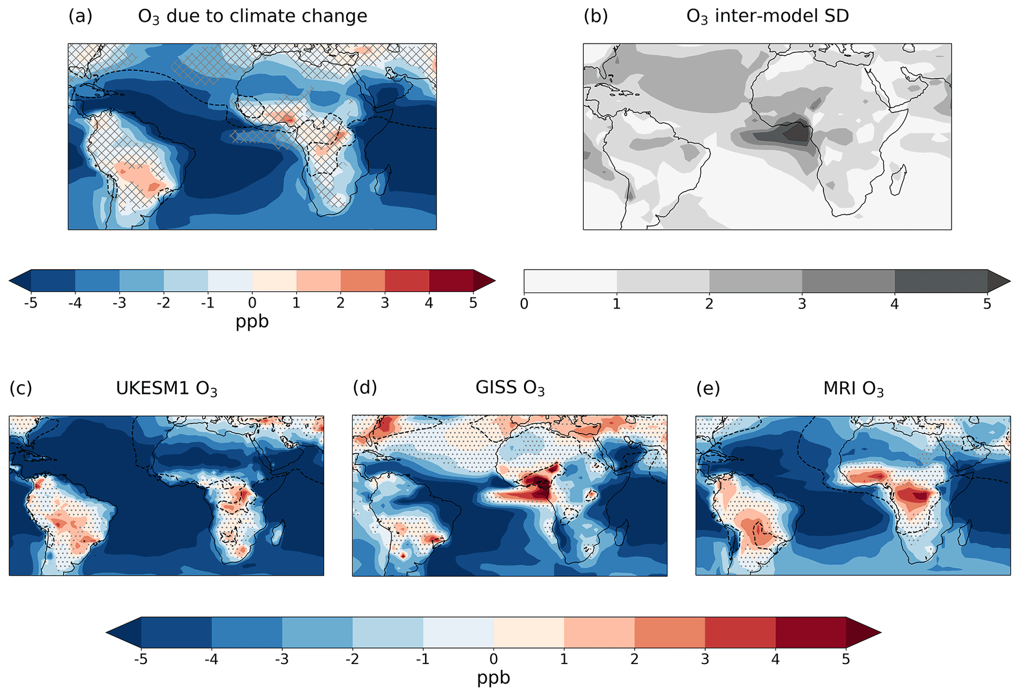
Figure 3 The average change in surface O₃ concentration due to climate change for the period 2090–2100 for (a) the multimodel mean, (c) UKESM1 only, (d) GISS only and (e) MRI only. Panel (b) shows the inter-model standard deviation in the same units. Grey hatching in (a) covers areas where the inter-model standard deviation is greater than 20 % of the multimodel mean value. Grey dots in panels (c–e) cover areas that are not significant at the 5 % level from Student's t test. Black dotted lines outline areas where background O₃ is higher than 40 ppb.

UKESM1 and MRI predict increases in surface O₃ concentration of up to 5 ppb in the Amazon and central Africa, with decreases over coastal regions due to climate change (Fig. 3c and e). In the remote Amazon, MRI predicts an increase and UKESM1 a decrease in O₃ concentration, but neither change is significant. On the other hand, GISS predicts significant O₃ decreases across remote regions of up to 4 ppb (Fig. 3d), including central Africa, which experiences O₃ increases in the other simulations (Fig. 3c and e).

Changes in surface O₃ concentration due to climate change in 2100 are shown in Fig. 4, grouped by regional biomass burning season, with dotted contours where background O₃ is 40 ppb (a number assumed to be associated with thresholds for plant O₃ damage) and 70 ppb. High background O₃ is associated with biomass burning and pollution in and around cities due to their higher NO_x emissions. These high-O₃ areas also show the greatest increase in O₃ due to climate change (Fig. 4).

Figure 4 The multimodel mean change in surface O₃ concentration due to climate change for the period 2090–2100 for (a) the western African burning season (December–February), (b) the southern African burning season (June, July), (c) the southern Amazon burning season (August–October) and (d) the remaining months with limited burning (March–May, November). Grey hatching covers areas where models disagree on the sign of the change due to climate change. Black dotted lines outline areas where background O₃ is 40 and 70 ppb.

During December–February, the biomass burning area in western Africa coincides with O₃ increases of 9 ppb (5 ppb for UKESM1, 7 ppb for MRI and 15 ppb for GISS; Fig. 4a), and similar O₃ penalties are seen for the southern African biomass burning season during June–July (Fig. 4b). During the Amazon biomass burning season, there are even larger increases of up to 12 ppb in the southern Amazon (Fig. 4c). In months without biomass burning, these areas have minor increases of 2 ppb for UKESM1 and MRI and a decrease of 3 ppb for GISS.

GISS is the only model to show significant decreases in monthly mean surface O₃ concentration over land, which consistently occur in areas and seasons with low background O₃ (not shown). This includes biomass burning areas but in seasons without burning, which are followed by large increases in the biomass burning season. The result is that seasonal changes in surface O₃ concentration due to climate change in GISS are much larger than UKESM1 and MRI, and models do not agree on the direction of change in remote areas, although the yearly average increase is similar between models (Fig. 3). This results in uncertainty in the response to climate change from regions and seasons with low background O₃ but likely increases in areas and seasons with high background O₃ from anthropogenic NO_x emissions (Fig. 4, black dashed lines).

Grid cells which include highly populated regions and megacities are often associated with an increase in O₃ concentration in all months and an average ozone–climate penalty of 3 ppb in the yearly average. In particular, there is an ozone–climate penalty of 3 ppb that shows limited seasonal variation in grid cells containing the megacities in Nigeria (Lagos), Brazil (São Paulo, Rio de Janeiro) and Colombia (Bogotá, Medellín). This penalty is robust over southeast Brazil in all seasons (Fig. 4).

3.4 Changes in chemical production and deposition of O₃ due to climate change

Attribution of changes in surface O₃ to changes in chemical production, chemical loss and dry deposition at the surface are shown in Fig. 5. The increase in O₃ production due to climate change is the largest of these terms (Fig. 5c) and increases the most (over 0.25 Tg yr⁻¹) in high-NO_x areas where surface O₃ increases (Fig. 5a). Therefore, the increase in the rate of O₃ production is likely to be the main cause of the ozone–climate penalty in high-NO_x areas (high-NO_x defined as in Fig. 1). Removal of O₃ by deposition and chemical destruction has a smaller effect on O₃ concentration since, to a degree, the two terms cancel each other out; in high-NO_x areas, chemical loss increases by up to 0.1 Tg yr⁻¹ and dry deposition decreases by up to 0.05 Tg yr⁻¹. In remote regions, there is considerable variation between models as indicated by the higher standard deviation in these areas (Fig. 5, column 2). GISS predicts decreases in O₃ production over remote regions of up to 0.1 Tg yr⁻¹ and increases of up to 0.25 Tg yr⁻¹ over high-NO_x regions, whereas MRI and UKESM1 predict increases in O₃ production across all regions except Saharan Africa. MRI predicts the largest increases in O₃ chemical production in remote areas of 0.25 Tg yr⁻¹ (not shown).

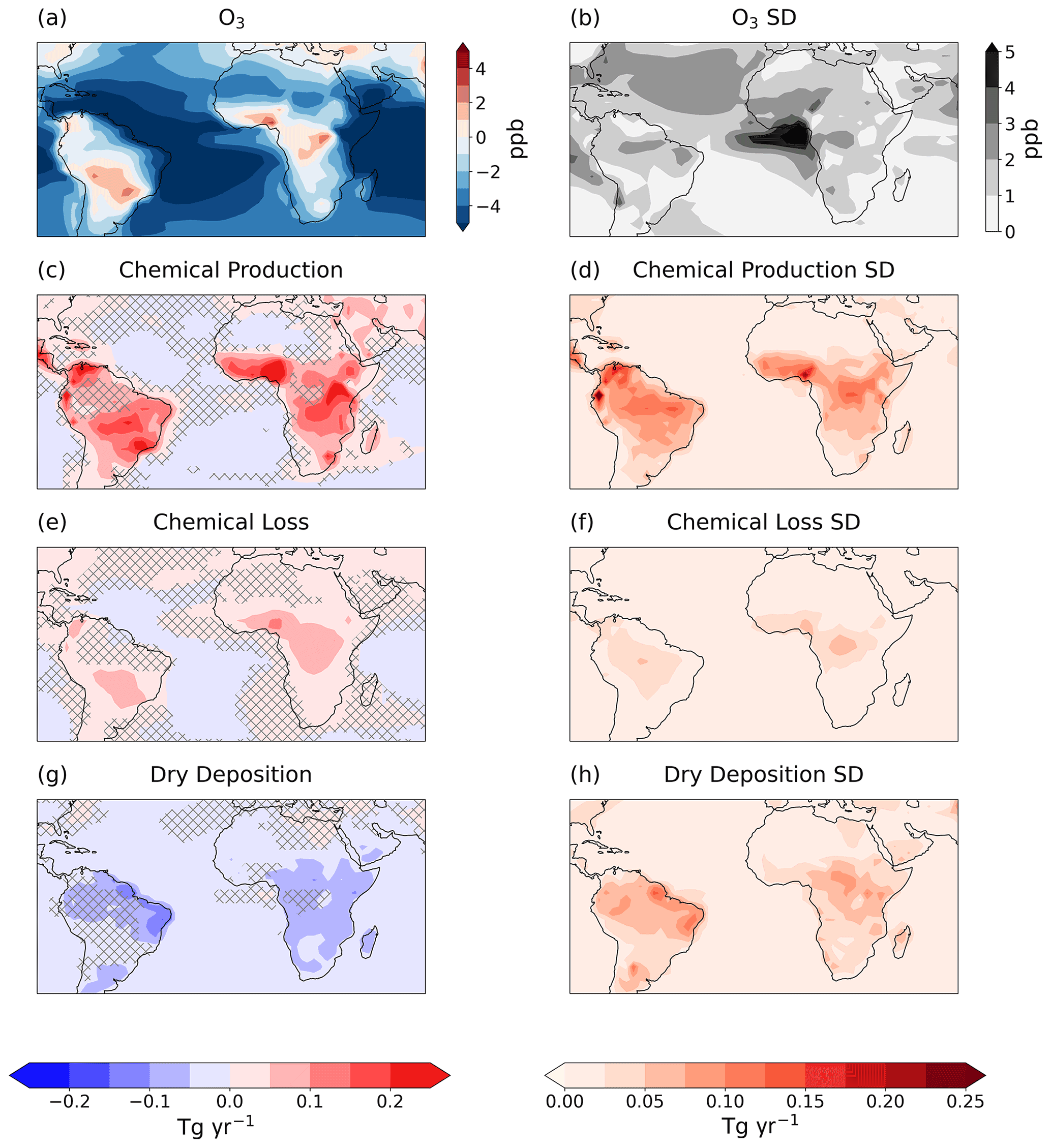
Figure 5 The multimodel mean change in (a) surface O₃ concentration, (c) chemical production of O₃, (e) chemical destruction of O₃ and (g) dry deposition of O₃ due to climate change. Panels (c), (e) and (g) show the change in O₃ in Tg yr⁻¹, and chemical terms have been summed over a 1 km height. The inter-model standard deviations are shown in panels (b), (d), (f) and (h).

Chemical loss and deposition changes become important in remote areas because these areas have the smallest increases in chemical production but can have the largest changes in loss rate (Fig. S8 in the Supplement) and deposition rate (Fig. S10 in the Supplement). The rate of O₃ loss is correlated with the change in isoprene concentration, which is typical of a low-NO_x region due to reactions between isoprene and O₃ directly (Fig. S8). This leads to increases in the loss rate in most vegetated areas (Fig. S8). Conversely, the deposition rate decreases, presumably because the increased temperatures and lower relative humidity cause stomatal closure. Dry deposition varies between each model depending on stomatal response to temperature changes and boundary layer resistance changes (Fig. S10). In UKESM1, the increase in CO₂ also reduces stomatal conductance. UKESM1 shows a large decrease in deposition rate over the central Amazon, whereas MRI shows very little change regionally.

In high-NO_x areas, the increase in O₃ production is greater than the increase in loss leading to net chemical production of O₃. Evaluation of the sensitivity of O₃ chemical production rate to changes in isoprene emissions and NO_x concentration due to climate change for each model is shown in Fig. 6 and described below.

Figure 6 (a–c) Surface NO_x concentrations in the absence of climate change and the average change due to climate change in (d–f) NO_x concentration, (g–i) isoprene emission rate and (j–l) O₃ production rate for the period 2090–2100 for (column 1) UKESM1, (column 2) GISS and (column 3) MRI.

Isoprene emission rate increases in both GISS and UKESM1 on average, as expected in a warmer climate (MRI does not have interactive isoprene emission) (Fig. 6, row 3). UKESM1 predicts a substantial decrease in isoprene emission rate in the northern Amazon and fractionally in west Africa (Fig. 6a). Decreases in isoprene emission and stomatal conductance have previously been simulated in the same area due to CO₂ inhibition (Pacifico et al., 2012; Chadwick et al., 2017; Turnock et al., 2020).

NO_x decreases in most areas in UKESM1 including high-NO_x areas, whereas GISS predicts increases of $\mathrm{2}\times {\mathrm{10}}^{-\mathrm{11}}$ to $\mathrm{6}\times {\mathrm{10}}^{-\mathrm{11}}$ mol mol⁻¹ in high-NO_x areas only and MRI predicts more uniform increases of $\mathrm{4}\times {\mathrm{10}}^{-\mathrm{11}}$ mol mol⁻¹ in all areas (Fig. 6, row 2). The magnitude of the background NO_x concentration in UKESM1 and the change due to climate change is also much larger than the other models. The negative NO_x concentration changes in UKESM1 and in some areas in GISS compared to MRI may be due to increased sequestration of NO_x into isoprene nitrates. This possibility is supported by evidence of anticorrelation between NO_x and isoprene in GISS and UKESM1 (Fig. 6). In GISS, the remote Amazon shows the largest isoprene increase and a decrease in NO_x concentration. UKESM1 also shows an increase in NO_x concentration downwind of the isoprene decrease in the northern Amazon.

Despite differences in the magnitude and direction of the NO_x and isoprene changes, the change in O₃ chemical production rate has similar spatial patterns in all models (Fig. 6, row 4). Exceptions occur in central Africa where GISS predicts a decrease in production rate and in Nigeria where UKESM1 is the only model that does not predict a large increase in O₃ production. These areas of Africa also exhibit differences in surface O₃ concentration between models, discussed in Sect. 3.3.

The O₃ production rate for GISS appears highly correlated with the change in NO_x concentration in Fig. 6e, whereas NO_x concentration decreases in many areas where O₃ production increases for UKESM1. Instead, isoprene may influence O₃ production in UKESM1. Areas with a decrease in isoprene emissions in UKESM1 also show a decrease or a smaller increase in O₃ production compared to other areas, suggesting isoprene is important for O₃ production in UKESM1 even in remote regions such as the northern Amazon.

To determine the strength of the relationship between O₃ production rate and changes in the precursors NO_x and isoprene, coefficients from a multiple linear regression are presented in Fig. 7. The monthly mean change in isoprene emission rate, NO_x concentration and O₃ production rate for each grid cell is shown graphically with locations and months of high-NO_x (above the 95th percentile) marked with stars. All three climate models produce coefficients between 0.33 and 0.41 for the relationship between changes in NO_x concentration and O₃ production rate (Fig. 7). However, the change in isoprene emissions using GISS and UKESM1 is a weaker predictor of O₃ production, even though increases in isoprene emission of over 100 % are predicted. All predictors are considered significant due to the large sample size, with r² values of 0.384, 0.732 and 0.590 for UKESM1, GISS and MRI respectively (Table S3 in the Supplement). The lower r² value for UKESM1 indicates that the changes in NO_x concentration and isoprene emissions explain less than half of the change in O₃ production rate. Additional analysis shows that the O₃ production rate in UKESM1 is also related to the background NO_x concentration (see Sect. S4: the relationship between NO_x and ozone production).

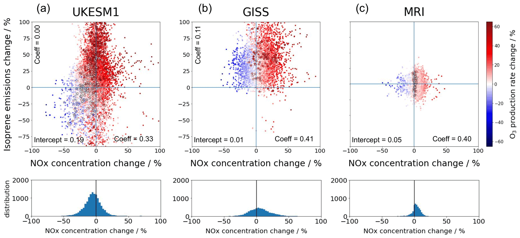
Figure 7 Scatter plots of the monthly mean percentage change in surface NO_x concentration, isoprene emission rate and O₃ production rate for each grid cell and each month for (a) UKESM1, (b) GISS and (c) MRI for the region 30^∘ S–30^∘ N, excluding Saharan Africa. Data for MRI have been randomly normally distributed along the y axis. Grid cells and months where the background NO_x concentration is greater than the 95th percentile for the region shown in Fig. 1 are marked with stars. The labelled intercept and coefficients refer to the results of a multiple linear regression ΔO₃ prod (%) ∼ ΔNO_x (%) + ΔIsoprene (%) using the plotted data. The second row contains the number of data points in each NO_x concentration change range. The data are divided into 50 bins.

GISS simulates increases and decreases in NO_x concentration of 50 %, compared to the smaller changes predicted by MRI, which fall mostly in the range 0 %–20 % (Fig. 7c). GISS therefore predicts decreases in O₃ production over remote regions (Fig. 6b) and seasons, whereas MRI predicts consistent increases (Fig. 6c). Additionally, high-NO_x areas simulated by GISS experience an increase in O₃ production regardless of the NO_x concentration change (Fig. 7b, stars). In high-NO_x areas simulated by UKESM1, the percentage change in NO_x concentration is small so there is not enough information to identify individual isoprene and NO_x sensitivities, although areas with increased isoprene emission also show increases in O₃ production rate (Fig. 7a, stars).

The apparent relationship between O₃ and isoprene in UKESM1 (Fig. 6) does not show up using a linear model (Fig. 7). A relationship may be hidden by variation in the isoprene–O₃ production sensitivity in different grid cells or by correlations between isoprene and NO_x (discussed further in Sect. S4: the relationship between NO_x and ozone production). However, as isoprene also contributes to O₃ loss, the effect of isoprene on net chemical production (production – loss) is reduced by the two terms cancelling each other out, so the change in net O₃ chemical production is more clearly related to the change in percentage NO_x concentration (Fig. S7 in the Supplement). In particular, the decrease in net O₃ production in the northern Amazon (Fig. S7d) resembles the percentage change in NO_x concentration (Fig. S7a) more than the percentage change in isoprene emissions (Fig. S7b).

The change in O₃ production rate will be further affected by meteorological changes, temperature in particular. This is the reason that O₃ production increases in UKESM1 and MRI even in the absence of changes in NO_x and isoprene (the intercepts of the linear model are 19 % and 5 % respectively) and O₃ production increases in areas showing decreasing NO_x concentrations in UKESM1. Since the temperature change varies seasonally and regionally, with dry seasons experiencing the largest increase in temperature, some of the changes in O₃ production in Fig. 7 may be driven by temperature rather than NO_x or isoprene changes. If isoprene/NO_x and O₃ production are both influenced by the underlying meteorology, the identified correlations may be due to meteorology rather than the chemical species changes. We verify that the monthly mean temperature change in each grid cell is not significantly correlated with percentage NO_x change in any model nor percentage isoprene change in UKESM1 (not shown). Therefore, NO_x and isoprene changes are likely controlled by many processes in addition to temperature, including background chemistry and emissions for NO_x and vegetation type and cover for isoprene, as well as other meteorological variables. This indicates that the identified correlations between NO_x and O₃ production are unlikely to be the result of a spurious relationship driven by temperature, although it is still possible that the strength of the correlations may be inflated by confounding meteorological variables.

4 Discussion

When compared to in situ observations, the three climate models used in this study overestimate present-day surface O₃ in tropical regions by 14 ppb on average, including 11 ppb over the oceans. This is close to the global bias of 16 ppb calculated by Turnock et al. (2020), which included data from six climate models, including the three in this study. Therefore, the sources of error may not be unique to the tropics and subtropics. The major sources of variation between model and observations are related to differences in the area sampled and the heights of the stations relative to the lowest model grid cell (Pacifico et al., 2015).

In the tropics and subtropics, we expect in-canopy deposition and chemical processes to be the most important contributor to the positive bias because these processes create a steep O₃ gradient at the surface, whereas models aim to predict O₃ concentrations at 20 m and above from the canopy top where these deposition processes are not included (Stroud et al., 2005; Gordon et al., 2014). Additionally, the volume of the model grid box is many times larger than the area sampled by measurement sites and also larger than the area of precursor emission sources such as fires. Therefore, the model inputs and predictions represent the average over a region that is not directly comparable with in situ measurements (Sinha et al., 2004). As a further validation, we also provide data from the TES satellite at 825 hPa, which records higher O₃ concentrations than the in situ sites since it measures at an altitude away from the canopy sink. Although this is much higher in altitude than the lowest grid box of any of the models, it should capture the above-canopy seasonal cycle at a resolution closer to the model grid resolution.

We find that the modelled surface O₃ bias compared to in situ observations is largest in biomass burning areas, although in South America the models capture the seasonal cycle well (Fig. 1). In situ sites, especially in the DR Congo (Fig. 1e), do not detect the large increases in O₃ predicted by models during biomass burning months, although observed O₃ concentrations are also highest during biomass burning season (Adon et al., 2013). A high positive bias during the dry season has been found in previous studies (e.g. Turnock et al., 2020), although our study has covered several regions that did not previously have available data. It is likely that effective removal within the canopy that is not included in models softens the observed seasonal cycle. In this region, the trends captured by satellites are closer to the model predictions, which increases confidence that models are correctly identifying O₃ enhancements above the canopy due to fires. However, future studies assessing the risks to human and ecosystem health should be aware of this limitation in current models.

The remainder of the study focuses on the change in surface O₃ due to climate change. Although model biases increase uncertainty in the change due to climate change, we quantify the difference between two simulations, which should remove systematic biases, and we note that the models capture seasonal and regional trends that are explained by either in situ measurements or satellite measurements (Fig. 1). This gives confidence in the trends in future O₃ change presented in this study, but we highlight O₃ from biomass burning as an area for further study. The models have different chemistry schemes, land processes and temperature sensitivities which contribute to model variation (Stevenson et al., 2006; Wu et al., 2007; Archibald et al., 2020b). For this reason, we do not attempt to completely diagnose reasons for inter-model variation and instead the aim of this study is to identify robust predictions and areas of uncertainty for the change in O₃ due to climate change.

We find that while overall O₃ concentrations over the tropical land areas are reduced under the climate scenario examined here, climate change could lead to an ozone–climate penalty in areas which have a high background NO_x concentration. These high-NO_x areas already tend to have high O₃ concentrations in the absence of climate change (above 40 ppb), with climate change causing a further deterioration in air quality. Models predict that climate change will lead to seasonal mean increases in surface O₃ concentration of up to 12 ppb in tropical and subtropical areas with high-NO_x emissions (Fig. 4). The increase in surface O₃ in high-NO_x areas is robust, with seasonal mean increases of up to 15 ppb for UKESM1, 18 ppb for GISS and 12 ppb for MRI. These areas are defined by NO_x emission magnitudes above the 95th percentile for the region 40^∘ S–40^∘ N, which is dominated by anthropogenic contributions such as biomass burning or urban emissions. O₃ pollution in forested areas has the potential to reduce forest productivity, decreasing the amount of carbon removed from the atmosphere and impairing forest resilience (e.g. Sitch et al., 2007; Grulke and Heath, 2020).

The ozone–climate penalty in high-NO_x regions is primarily driven by an increase in O₃ chemical production, which is largest in areas of high NO_x (Figs. 5 and 6). This is in agreement with results from Doherty et al. (2013) and Archibald et al. (2020b) who showed that the rate of change of O₃ with temperature increases with NO_x concentration. Firstly, the major O₃-forming reaction $\mathrm{NO}+{\mathrm{HO}}_{\mathrm{2}}/{\mathrm{RO}}_{\mathrm{2}}$ happens faster at higher temperatures, and scaling up O₃ production in an area where O₃ production is already high will often lead to greater O₃ increases than an area with low-O₃ precursor concentrations (Coates et al., 2016). Secondly, VOC and NO_x concentrations can increase at higher temperatures. NO_x concentration can increase due to increased PAN decomposition at higher temperatures (Doherty et al., 2013), changes in lightning frequency or changes to atmospheric chemistry, and VOCs increase largely as a result of increased isoprene emissions. All models likely exhibit an increase in reaction rates; however there were differences between UKESM1 and the other models in their sensitivity to changes in NO_x concentration and isoprene emissions (Fig. 7).

Using a multiple linear regression, we find that changes in NO_x concentration are strongly correlated with changes in O₃ production rate for GISS and MRI (r²=0.732 and 0.590 respectively) (Fig. 7). For UKESM1, we find that linear regression using changes in NO_x concentration and isoprene emission explains less than 50 % of the change in O₃ production rate. Including background NO_x concentration in the linear regression improves the r² value and suggests that the rate of O₃ production increases in proportion to the background NO_x concentration (Fig. S5 in the Supplement). UKESM1 has previously been identified as being among the least responsive to changes in precursor concentrations out of the CMIP6 models (Turnock et al., 2020), and indeed chemical production increases in many areas despite decreases in NO_x, so the increase in chemical O₃ production is more likely to be dominated by an increase in the rate of reaction and not changes in precursor concentration. The linear regression uses monthly means, so modelled O₃ increases during burning seasons (dry seasons) are likely compounded by the fact that these seasons often show the greatest temperature increase due to climate change (Fig. S3). Therefore, some of the identified correlations may be due to meteorology changes rather than chemical changes.

As changes in NO_x concentrations are shown to be important for changes in O₃ production in GISS and MRI, we now discuss the inter-model differences in NO_x concentration changes in further detail. GISS and MRI agree that NO_x concentrations will increase in high-NO_x regions but disagree on the direction of change in remote regions. UKESM1 predicts a decrease in NO_x concentrations in many areas. GISS predicts a decrease in NO_x of $\mathrm{2}\times {\mathrm{10}}^{-\mathrm{11}}$ mol mol⁻¹ in remote areas (up to 50 %) while MRI predicts an increase of $\mathrm{2}\times {\mathrm{10}}^{-\mathrm{11}}$ to $\mathrm{6}\times {\mathrm{10}}^{-\mathrm{11}}$ mol mol⁻¹ in remote regions. This is likely causing the difference in O₃ production between GISS and MRI in remote regions. To reduce uncertainty in predictions for O₃ concentration changes due to climate change, further work to constrain future NO_x concentration changes is needed.

The NO_x concentration change depends on the balance of NO_x production and loss terms. A large contributor to increases in NO_x concentrations in all models is an increased decomposition of PAN into NO_x, which will be largest in source regions. Lightning NO_x is also a NO_x source, but its influence on surface NO_x remains unclear. Although lightning NO_x increases in all models during the wet season, the largest surface NO_x and O₃ increases occur in the dry season, so the ozone–climate penalty is unlikely to be driven by lightning NO_x changes. Nevertheless, the large increase in lightning NO_x in MRI may have a role in the increase in surface NO_x concentration in MRI, which is larger than the other models, and lightning NO_x decreases in the northern Amazon during the dry season (Fig. S4a) may contribute to the decrease in NO_x and O₃ production in this region in UKESM1 (Fig. S7). A large contributor to the loss term will be reaction with isoprene derivatives and thus increased formation of isoprene nitrates. In both UKESM1 and GISS, isoprene and NO_x are anti-correlated in some areas, suggesting isoprene emission changes have a notable effect on NO_x concentrations. For example, GISS predicts large isoprene increases in the remote Amazon, where the major NO_x decreases occur, and UKESM1 shows a small area of increased NO_x concentrations downwind of the northern Amazon, where isoprene decreases. As MRI prescribes isoprene as a climatology, there will be no significant change to NO_x loss via organic nitrate formation and this is likely a reason why NO_x increases over most areas of land. The reasons why NO_x loss dominates in UKESM1, whereas GISS shows a net NO_x increase requires further understanding of individual model details such as isoprene nitrate yield and NO_x recycling frequency. The sensitivity of NO_x concentration to changes in lightning, PAN and isoprene in each model is beyond the scope of this study but would be useful to explore in further work. Further studies could also explore some temperature-sensitive sources of NO_x that were not included in the simulations such as soil NO_x emissions and changes in wildfire frequency.

NO_x is not the only driver of changes in O₃ production, and changes in temperature-dependent emissions of isoprene also influence the rate. This may be especially important in UKESM1, which predicts the highest concentration of background NO_x because high-NO_x areas may experience a different chemical regime in which VOCs also increase O₃ production (e.g. Liu et al., 2021). For example, UKESM1 shows increases in O₃ production rate as isoprene increases in high-NO_x areas (Fig. 7, stars). However, calculating the net effect of isoprene on surface O₃ concentrations is complex; increasing isoprene emissions can increase both the rate of O₃ production and the rate of O₃ loss and, as described above, can decrease concentrations of NO_x and OH. Examining the percentage change in net O₃ chemical production in UKESM1 (Fig. S7) suggests the net effect of changing isoprene emissions on O₃ chemistry cancel out and that the percentage change in net O₃ production is more closely related to percentage changes in NO_x concentration.

The increase in chemical loss is strongly correlated with isoprene concentration change in UKESM1 and GISS (Fig. S8). Therefore, the different isoprene schemes used by each model contribute to uncertainty in the loss rate over the continents. In particular, MRI used climatological isoprene resulting in no significant change in the loss rate (Fig. S8c), and UKESM1 includes CO₂ inhibition, which decreases the isoprene emission rate and loss rate in northern Amazonia (Fig. S8a). Overall, this means that GISS has a higher loss rate, especially in low-NO_x, high-isoprene regions such as the remote Amazon, which may partly account for the larger decreases in O₃ in remote regions using this model (Fig. 3).

The global study by Zanis et al. (2022) employs two additional climate models and also finds climate benefits and uncertainties in surface O₃ concentrations in the same remote regions. We excluded these two models from our own study as data for the sensitivity study (NO_x concentration and isoprene emission rate) were not available at the time of writing. Zanis et al. (2022) highlight the different isoprene emission schemes as a reason for model variation; however our analysis (Fig. 7) finds NO_x to be the most important precursor. The fact that the models contain positive correlations between the change in NO_x and O₃ production, and between the change in isoprene and O₃ loss, indicates the tropics and subtropics exhibit NO_x-limited behaviour, although isoprene may be important in high-NO_x areas. We agree that isoprene is highly relevant for the change in loss rate and for indirect effects on O₃ through changes in related atmospheric chemistry such as OH and NO_x concentrations.

The decrease in deposition rate is controlled by UKESM1 and GISS (MRI showed very little change), but there was spatial variation in the magnitude of the change. This could be due to changes in meteorology between models (such as temperature and precipitation), as well as model differences (UKESM1 includes CO₂ inhibition). Feedbacks such as O₃ damage to vegetation were not considered in any model (Pacifico et al., 2015) but may be a useful addition to future simulations.

Models tend to predict a decrease in surface O₃ over regions strongly affected by ocean air such as north Brazil. This is due to robust decreases in O₃ over the oceans from increases in atmospheric water vapour. Over land, increases in water vapour and OH influence the concentrations and lifetimes of many species.

We finally note that Nigeria experiences substantial increases in O₃ production according to GISS and MRI, whilst a slight decrease is predicted using UKESM1. This is an important geographical area for future research since poor air quality could affect large numbers of people living in west African cities. In this area, the choice of emission scenario is also important for determining the O₃ response to climate change because NO_x emissions in Nigeria increase rapidly in the SSP3-7.0 scenario compared to the present-day due to predicted urbanisation. Therefore, future studies should explore alternative emission pathways to better inform policy.

5 Conclusion

Using a multimodel mean of data from three Earth system models, we identify that by 2100, there will be an ozone–climate penalty in high-NO_x areas, such as major cities and biomass burning areas (Fig. 4). This is not due to increased fire emissions but due to the increasing temperature, which speeds up the recycling of NO into NO_x and increases decomposition of PAN into NO_x in source regions. It shows that the ozone–climate penalty is greatest in areas already experiencing high O₃, putting forests in these areas at greater risk of O₃ damage and urban populations at increasing threat of health problems. This study adds to findings from the World Health Organisation World Air Quality Report (2021) that air pollution is an increasing issue across the tropics and that there is a need for greater monitoring of air pollution across Africa and South America.

The Earth system models display NO_x-limited behaviour, including that higher NO_x concentrations lead to increased O₃ chemical production and therefore increased surface O₃ concentration (Figs. 5–7). As the background concentrations of NO_x are largely anthropogenic, this suggests that without reduction in emissions, forested areas in urban and fire-prone locations are more at risk from increases in surface O₃ due to climate change than remote forests. As O₃ damage can reduce plant productivity, this has implications for the success of secondary forests and other human-modified forests, which are mostly located in agricultural areas, deforestation frontiers and forest edges (Heinrich et al., 2021) and may reduce their carbon sequestration potential (Sitch et al., 2007).

In remote regions, differences in the direction of O₃ concentration change between models creates uncertainty as to whether remote locations are at greater risk of O₃ damage in a warmer climate, although ocean-influenced areas display robust climate benefits (Fig. 4). Further work is needed to constrain the climate response of isoprene emissions and the temperature sensitivity of NO_x and O₃ chemistry.