the Creative Commons Attribution 4.0 License.
the Creative Commons Attribution 4.0 License.
 | 20 Sep 2022
Life cycle of stratocumulus clouds over 1 year at the coast of the Atacama Desert
Camilo del Rio
Juan-Luis García
Pablo Osses
Sarah Westbrook
Ulrich Löhnert
Marine stratocumulus clouds of the eastern Pacific play an essential role in the earth's energy and radiation budget. Parts of these clouds off the western coast of South America form the major source of water to the hyperarid Atacama Desert coastal region at the northern coast of Chile. For the first time, a full year of vertical structure observations of the coastal stratocumulus and their environment is presented and analyzed. Installed at Iquique Airport in northern Chile in 2018/2019, three state-of-the-art remote sensing instruments provide vertical profiles of cloud macro- and micro-physical properties, wind, turbulence, and temperature as well as integrated values of water vapor and liquid water. Distinct diurnal and seasonal patterns of the stratocumulus life cycle are observed. Embedded in a land–sea circulation with a superimposed southerly wind component, maximum cloud occurrence and vertical extent occur at night but minima at local noon. Nighttime clouds are maintained by cloud-top cooling, whereas afternoon clouds reappear within a convective boundary layer driven through local moisture advection from the Pacific. During the night, these clouds finally re-connect to the maritime clouds in the upper branch of the land–sea circulation. The diurnal cycle is much more pronounced in austral winter, with lower, thicker, and more abundant (5×) clouds than in summer. This can be associated with different sea surface temperature (SST) gradients in summer and winter, leading to a stable or neutral stratification of the maritime boundary layer at the coast of the Atacama Desert in Iquique.
- Article
(8305 KB) - Full-text XML
- BibTeX
- EndNote


Stratocumulus clouds cover, averaged over the year, about 23 % of the oceans and 12 % of the land surface, making them the most abundant cloud type (e.g., Wood, 2012). As they reflect between 30 % and 60 % of the incoming solar radiation, they have a cooling effect and play an important role in the radiation budget of the planet. Large stratocumulus cloud fields can be typically found at the western coasts of the continents, where equatorward cold ocean currents like the Humboldt and Benguela currents meet stable atmospheric stratification mediated by the subsiding branch of the Hadley circulation. Under these conditions, a persistent stratocumulus cloud deck forms with a mixed maritime boundary layer (MBL) and an extremely sharp inversion above, separating the cloud layer from the free troposphere. This system is stabilized by several feedback mechanisms: radiative and evaporative cooling at the cloud top initiates turbulent mixing between cloud and ocean surface. Evaporation from the ocean and mixing through the boundary layer provide a continuous flow of water vapor balancing the water loss at the cloud top (e.g., Schubert et al., 1979; Stevens et al., 2003) and precipitation back into the ocean (Wood, 2012). It has been hypothesized that evaporative cooling at the cloud top may increase turbulent exchange between the moist boundary layer and the dry, free troposphere and thus dissipate the cloud (cloud-top entrainment instability, CTEI), but it has been found that this mechanism requires special conditions and occurs less frequently than originally thought (Wood, 2012). The stratocumulus in the southeastern Pacific off the coast of Peru and northern Chile has been identified as having the largest geographical extent and being the most persistent in the world (Klein and Hartmann, 1993). In addition to their global role, these clouds provide fresh water to coastal ecosystems in the form of fog in deserts like the Atacama (e.g., Muñoz-Schick et al., 2001; Cereceda et al., 2008a; Manrique, 2011). Due to the extreme aridity in the Atacama, this is the only significant water source and, accordingly, it determines several processes, from genetic evolution to surface mineral formation (Dunai et al., 2020).
The mechanisms behind the formation and persistence of maritime stratocumulus have been investigated in many model studies from the first bulk-layer model of Lilly (1968) and its improvement by including moist thermodynamics (Schubert et al., 1979) or allowing a decoupling of the ocean from the cloud (Turton and Nicholls, 1987). These bulk models rely on basic physical principles like conservation of energy and matter. They assume a well-mixed layer between surface and cloud top and need parameterizations of the turbulent surface and entrainment fluxes. Global or regional circulation models cannot resolve structures of the stratocumulus clouds or the microphysical processes within the cloud, but they allow one to investigate their role in the local or global climate. An investigation of stratocumulus clouds in models of the Coupled Model Intercomparison Project (CMIP5) revealed that these state-of-the-art climate models have problems in representing stratocumulus above the southeastern Pacific correctly (Lin et al., 2012). When comparing to observations, these models showed a too low cloud cover, too high cloud tops, and non-realistic cloud reflectivities. Reasons for these shortcomings were identified as the turbulence driven by radiative cooling at the cloud top, which is not represented in most of the models, as well as the sharp inversion at the top of the MBL which cannot be resolved by these models (Lin et al., 2012, and references therein).
The hope would be that the latter problems could be solved by large eddy simulation (LES). These models resolve the large turbulent eddies mediating the transport in the MBL and parameterize the small-scale turbulence based on the structure of these large-scale eddies. A study comparing several LES models against observations showed that these models overestimated the turbulent mixing and thus entrainment at the cloud top (Stevens et al., 2005). As a result, water contents were too low and the cloud decoupled from the underlying MBL. The authors identified as reasons for the too strong entrainment a too low (vertical) resolution at the cloud top and insufficient understanding of subgrid-scale physics in this very region. Despite these difficulties, LES models can reveal insight into processes which cannot be resolved with global circulation models. For example, Schneider et al. (2019) show that a drastic increase in CO2 could lead to a breakup of the large stratocumulus fields above the oceans and that this breakup could only be reversed when returning to pre-industrial CO2 levels.
As even LES models cannot represent all aspects of stratocumulus cloud processes, one has to rely on observations. The stratocumulus at the western coast of North America has been investigated during several campaigns from ships and airplanes like the Dynamics and Chemistry of Marine Stratocumulus (DYCOMS) field studies (e.g., Stevens et al., 2003), which focused on the dynamics, especially the entrainment at the cloud top. Measurements were made from airplanes during dedicated days. The Marine ARM GCSS Pacific Cross-Section Intercomparison (GPCI) Investigation of Clouds (MAGIC) field campaign used remote sensing instrumentation on a ship to investigate the structure of the stratocumulus cloud deck off the western coast of North America, i.e., its longitudinal gradient (Zhou et al., 2015).
The EPIC and PACS Stratus 2003 and 2004 campaigns (Serpetzoglou et al., 2008; Bretherton et al., 2004) as well as the VAMOS Ocean-Cloud-Atmosphere-Land Study Regional Experiment (VOCALS-REx) used a whole set of observations from maritime platforms like ships, airplanes, and satellites to investigate the structure of the southeastern Pacific stratocumulus west of the coast of Peru and northern Chile (Wood et al., 2011; Mechoso et al., 2014). The goal of these campaigns was to increase the understanding of the coupling between ocean surface and atmosphere and cloud–aerosol–precipitation interactions. All these campaigns were limited in time.
To investigate the long-term development of the stratocumulus of the southeastern Pacific, Schulz et al. (2012) and Muñoz et al. (2016) analyzed airport observations of the cloud base from the three coastal Chilean airports of Arica (18.5∘ S), Iquique (20.5∘ S), and Antofagasta (23.7∘ S). Cloud occurrence shows a clear diurnal and seasonal pattern with maxima during the night in winter and spring. While Schulz et al. (2012) found a weak decrease in cloud cover, Muñoz et al. (2016) were able to show that, with higher temporal resolution and restriction to low clouds only, a long-term increase in spring and decrease in fall as well as a cloud base decrease of 100 m per decade can be found. A similar pattern in cloud cover can be found in satellite data, with a weak increase in cloud cover in winter and spring, especially over the ocean, and a decrease above land with altitudes above 1000 m a.s.l. (above sea level) (del Rio et al., 2021a). Besides these weaker long-term trends, cloud cover shows a strong inter-annual variability which is connected to the El Niño–Southern Oscillation (ENSO) global circulation pattern with opposite effects in different seasons. During an El Niño phase with warm equatorial waters, cloud cover is, in comparison to other years, increased in summer and decreased in winter and vice versa in La Niña years (del Rio et al., 2021a).
To date, no continuous, long-term observations of the vertically resolved dynamic, thermodynamic, and microphysical properties of these coastal stratocumulus and their environment exist. These parameters are important for quantifying heating rates and understanding the cloud life cycle and would provide valuable information for model evaluation and development of parameterization schemes. We present here data from a 1-year deployment of three state-of-the-art remote sensing instruments at the airport of Iquique (Chile, 20.54∘ S, 70.18∘ W) as part of the German Research Foundation (DFG)-funded collaborative research center 1211 “Earth – Evolution at the Dry Limit” (https://sfb1211.uni-koeln.de, last access: 2 September 2022) in close cooperation with the Centro del Desierto de Atacama (Pontificia Universidad Católica de Chile, UC).
The main objective of this paper is to quantify and understand the very pronounced diurnal cycle of these coastal stratocumulus clouds and relate it to the seasonal differences in sea surface temperature (SST) and the large-scale flow. In addition, we investigate mechanisms which transport water vapor and heat into or out of the cloud. Specifically, stratocumulus clouds show strong evaporation at their top and may lose liquid water by drizzle. The related water loss must be compensated by transport of water vapor from the ocean surface. The interplay of these processes is still not very well understood (see Wood, 2012), and our dataset provides insights by revealing details of the atmospheric boundary layer below the stratocumulus.
The paper is structured as follows: Sect. 2 describes the Iquique Airport site as well as the deployed instrumentation. The retrievals used to derive the atmospheric and cloud properties are briefly described. Section 3 presents statistics of the obtained observations in order to characterize diurnal and yearly variability of the stratocumulus, and finally Sect. 4 provides a scientific discussion of the observed stratocumulus life cycle at the Atacama Desert coastline.
2.1 Measurement site Iquique
The instruments were deployed from March 2018 to March 2019 on the grounds of the airport of Iquique at the coast of northern Chile at 20∘32′22′′ S, 70∘10′38′′ W about 2.5 km from the coastline (Fig. 1). The period is characterized by a return from a rather weak La Niña phase ending in April 2018 (Oceanic Niña Index ONI = −0.7) and a comparably weak El Niño phase beginning in October 2018 and lasting until June 2019 (average ONI = 0.7 with maximum ONI = 0.9 around November 2018; see NOAA Climate Prediction Center, 2022). The airport is located on flat terrain at about 56 m a.s.l. between the ocean and the coastal mountain range, which forms here an about 400 m-high cliff that lies 4 km from the coastline. The site is especially characterized by its location at the northern end of a coastal plain which extends about 30 km to the south, is 2 to 4 km wide, and is between 20 and 50 m above the ocean. This is a somewhat unique setting at the coast of northern Chile, as the cliff usually drops from several hundred meters directly into the ocean, with only narrow stretches of rocky beaches. The cliff is part of the coastal mountain range, with further inland heights around 1100 m and summits around 1400 m a.s.l. The stratus cloud thus interferes with the topography within a few kilometers, provides fog water to the surface, and is limited in its extension to the east (blue and red lines in Fig. 1). About 120 km to the east rise the Andes to heights above 5000 m, forming the western border of the Altiplano, a plateau at 3800 m with the salt pan of the Salar de Uyuni. Between the Andes and the coastal mountain range lies a central valley at heights around 1000 m. In the area between the coast and the Andes lies the Atacama Desert.
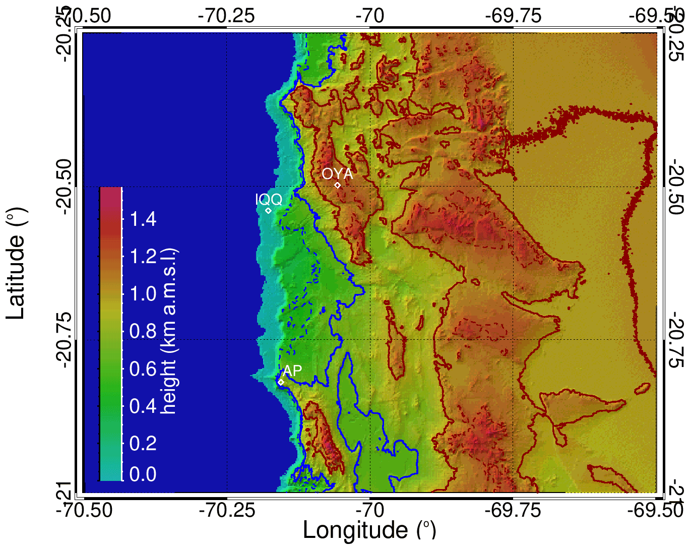
Figure 1Topography map of the region around the measuring site at Iquique (IQQ) Airport. IQQ depicts the location of the instruments, OYA is the position of the main meteorological station of the Oyarbide site, and AP is the Alto Patache UC desert research station. Lines indicate the elevation range of the stratocumulus cloud as we observed it in this study from IQQ. Blue and red lines show cloud-base and cloud-top height, respectively. Solid lines indicate the average and dotted lines the average ± standard deviation.
Besides the logistical advantages of an airport (electricity, communication, and safety), an additional reason for the choice was the proximity to the Oyarbide site (operated by Pontificia Universidad Católica UC and Heidelberg University) a few kilometers inland with standard meteorology and fog collectors (García et al., 2021; del Rio et al., 2021b). Standard meteorological observations from the airport were used in Schulz et al. (2012) and Muñoz et al. (2016) to evaluate long-term trends of stratocumulus clouds in the eastern Pacific.
The airport of Antofagasta about 320 km to the south hosts a radiosonde station (WMO ID 85442). Launch is every day at 12:00 UTC, i.e., about 2.5 h after sunrise. Data from these soundings have been used to derive statistical retrieval algorithms for the deployed microwave radiometer (Sect. 2.2.2). Three remote sensing instruments were deployed: a microwave radiometer (MWR), a cloud radar (CR), and a Doppler wind lidar (DL). Additionally, two simple meteorological stations at heights of 1 and 2 m above ground were installed.
2.2 Instruments
2.2.1 Radar
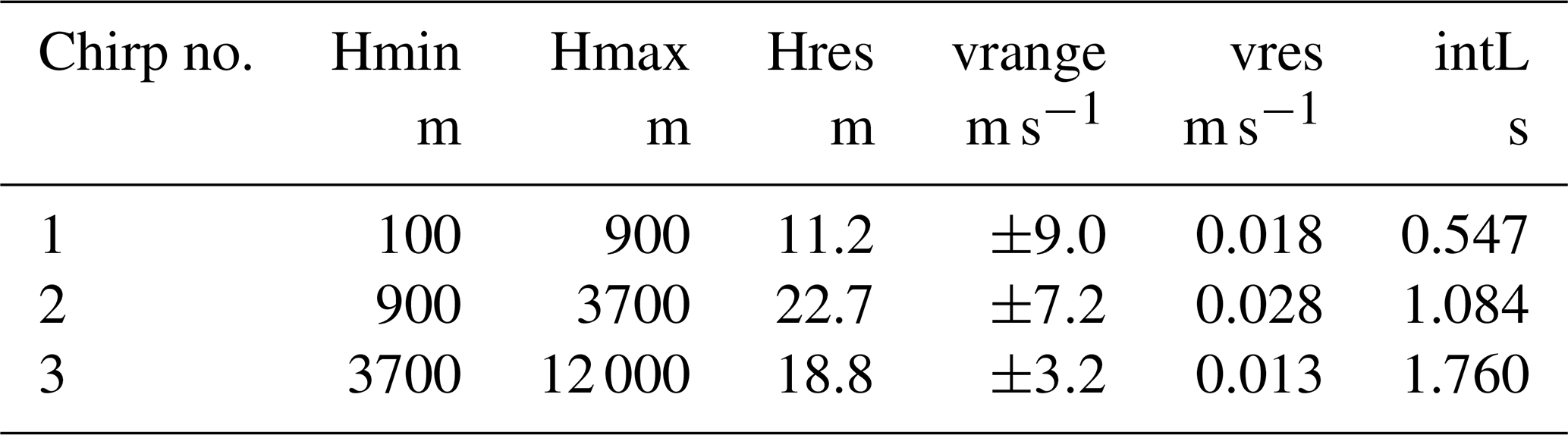
The cloud radar is a frequency-modulated continuous-wave (FMCW) radar RPG-FMCW-94 manufactured by RPG GmbH (Meckenheim, Germany, Küchler et al., 2017). The instrument was installed so that the radar beam is oriented vertically. The frequency of the emitted radar waves is modulated around 94 GHz in a saw-tooth pattern resulting in reoccurring so-called chirps. In the radar software, the user can define the dependent parameters height range and resolution as well as velocity range and resolution, which determine the chirp parameters for the instrument. To cover the height range from 0.1 to 12 km, we defined three different chirps. Height ranges of the different chirps were adapted to the expected heights of the stratocumulus. Each of the chirps is repeated between 6000 and 9800 times, leading to a total integration time of 3.39 s before the chirp sequence is repeated. Height and velocity ranges and resolutions as well as integration time per chirp are depicted in Table 1. From the backscattered and received signal, the CR derives Doppler velocity spectra, a radar reflectivity factor Ze, mean and standard deviation, as well as skewness of the Doppler velocity spectrum.
Table 1Main parameters of the chirps used by the cloud radar. Hmin, Hmax and Hres are minimum, maximum and resolution of the height, vrange and vres are velocity range and resolution, respectively, and intL is the integration time over each chirp.
2.2.2 Microwave radiometer
The microwave radiometer is a HATPRO (Humidity And Temperature PROfiler, Rose et al., 2005) manufactured by RPG GmbH (Meckenheim, Germany). It measures thermal radiation as brightness temperatures (TBs) in the microwave range in seven channels at the oxygen emission line complex at 60 GHz (W Band) and seven more channels at the higher flank of the 22.2 GHz water vapor emission line (K band). Zenith TBs are measured every second. From these brightness temperatures integrated water vapor (IWV), liquid water path (LWP), temperature profiles, and water vapor profiles are derived. The instrument was calibrated against liquid nitrogen at the beginning of the campaign. To ensure stability, the instrument performs frequent internal calibrations against a noise diode and a hot load kept at a controlled temperature.
Retrievals to derive the atmospheric variables from the TB are based on multivariate regressions based on the 14 TB channels (Löhnert and Crewell, 2003; Crewell and Löhnert, 2007). A multi-year radiosonde dataset is used to simulate the 14 TB channels via a line-by-line radiative transfer model. Specifically, we used 20 years of data from the nearest radiosonde in Antofagasta (4297 profiles from 1998 to 2018, i.e., 67 % of all data after a thorough quality control). The simulated TBs are related to the corresponding atmospheric variables using a quadratic minimization. The resulting regression coefficients are then used to derive the atmospheric variables from TB measurements at Iquique.
To improve the accuracy of the temperature profiles, so-called boundary layer scans are performed every 15 min. These scans are performed in the vertical plane at 70∘ azimuth and consist of 19 elevation angles with nine elevations from 4.2 to 30∘, a zenith observation, and symmetrical elevations on the opposite side. The scan thus ran from a direction to the Oyarbide measuring field towards the ocean. The idea was to eventually investigate differences in stratification towards the ocean and towards the mountains. Unfortunately, the lowest-elevation angles were lower than the line of sight towards the cliff, and the inland half of the scan could not be analyzed meaningfully. For this reason, only the scans towards the ocean were used for this enhanced temperature profiling. These boundary-layer scans allow derivation of temperature profiles with low uncertainty (<0.5 K root mean square error – RMSE) in the lowest 100 m, increasing further up to the middle troposphere (1.5 K RMSE; see Crewell and Löhnert, 2007). Water vapor profiles are vertically coarsely resolved using MWR measurements; i.e., there are only approximately two independent pieces of information contained in the TBs for water vapor profiling (Löhnert et al., 2009).
An intrinsic feature of passive remote sensing is that spatial resolution decreases with distance. As a result, the inversion appears much broader than it is in reality, and it becomes impossible to identify the bottom and top of the inversion layer. It will also be difficult to identify a moist adiabatic temperature profile in a cloud layer of a few hundred meters directly below the inversion. To estimate the height of the inversion, we first identify the maximum potential temperature gradient, fit a second-order polynomial to the three gradient values around, and determine the location of the maximum of this polynomial as the height of the inversion.
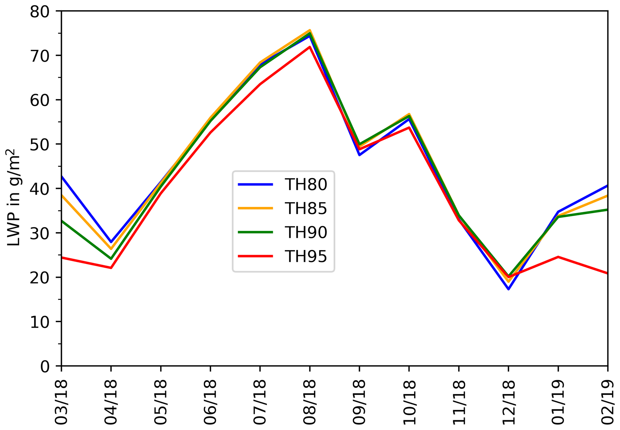
LWP is not directly measured by the radiosonde used for calibration but must be diagnosed from relative humidity and temperature. It is assumed that condensation occurs and a cloud forms when relative humidity (RH) exceeds a threshold RHcld. Liquid water content in the cloud is assumed to follow a modified moist adiabat (Karstens et al., 1994) and is finally integrated to provide LWP. This method can introduce some systematic LWP offsets in comparison to real clouds, especially if thin cloud layers like stratocumulus are present. Additionally, the vertical resolution of radiosonde profiles from Antofagasta prior to about the year 2000 is very low. As a result, the standard threshold of RHcld=95 % leads to complete years diagnosed with no or only a few clouds. A comparison of the vertical frequency distributions of clouds from the Cloudnet classification scheme derived from our 2018/2019 data (Sect. 2.3.1) to a cloud distribution from the radiosonde based on different RH thresholds revealed that for every year a different threshold would be necessary. Given the uncertainty of this method, we decided to calculate LWP with four different retrievals based on the four thresholds 80 % (TH80), 85 % (TH85), 90 % (TH90), and 95 % (TH95) in RH. The differences between the four thresholds thus give a measure of the uncertainty for the special situation at the Iquique Airport site.
2.2.3 Doppler lidar
The Doppler wind lidar deployed is a Streamline XR from HALO Photonics (Worcestershire, UK). It sends laser pulses at a wavelength of 1500 nm at a rate of 10 kHz into the atmosphere, measures the backscattered signal, integrates over 1 s, and derives the along-beam mean Doppler velocity and backscatter coefficient at 30 m spatial resolution. The maximum range is 15 km, but the Doppler signal detection needs sufficiently strong backscatter, which typically limits the applicable range to the atmospheric boundary layer with higher aerosol contents. The instrument performed a conical scan at an elevation of 70∘ every 15 min and at 24 azimuth angles (VAD scan) to derive a vertical profile of the horizontal wind vector based on the method described in Päschke et al. (2015). This scan was followed by a scan in the same vertical plane as the MWR (RHI scan). During the remaining time between scans, it measured vertical velocities at a temporal resolution of 1 s to characterize the turbulence in the boundary layer. These vertical measurements sum up to 52 min 44 s per hour and are used for an uncertainty estimate of the horizontal winds as well as for the boundary-layer classification scheme described in Sect. 2.3.2. Vertical backscatter measurements are used to derive the cloud base (Sect. 2.3.1).
2.2.4 Standard meteorology
Both the MWR and CR are equipped with a standard weather station (WXT 530, Vaisala, Finland). The station measures air pressure, wind speed and direction, temperature and relative humidity, as well as precipitation, providing values every 1 (MWR) and 4 s (CR), respectively. The two stations are mounted at 2.25 and 1.25 m and thus give information about the near-surface stratification.
Intercomparison of air temperatures (Ta) from our instruments and the operational airport measurements (Direccion Meteorologica de Chile Servicios Climaticos, 2022), about 1.5 km to the south, reveals good agreement with differences within ±0.5 K. An exception to this is summer, when temperatures rise above about 22 ∘C and our Ta is on average 0.5 K higher. This excess can be explained by the lack of an active ventilation in our measurements. Dew point calculated from our instruments is systematically 0.8 K lower than from the airport data, with scatter on the order of 0.3 K. This is equivalent to 3 percent points too low readings in our relative humidity measurements. Although this is within the range of the instruments' accuracy, we corrected this difference.
2.2.5 Sea surface temperature
We use two global SST datasets (Naval Oceanographic Office, 2008, 2018), both with 0.1∘ and 1 d resolution, to investigate the influence of the ocean. They are based on merged observations by different instruments on different satellites. For times until 15 January 2019, Naval Oceanographic Office (2008) has been used, and for times after 15 January 2019, Naval Oceanographic Office (2018) has been used. The datasets overlap between October 2018 and January 2019, and values in the region around Iquique show no differences during this time. From these datasets we extract two single-pixel time series 5 km west of the airport in the ocean (20.5∘ S, 70.2∘ W) and 50 km to the southwest in the open ocean (21.0∘ S, 70.7∘ W) (Fig. 2).
2.3 Synergistic retrievals
2.3.1 Cloudnet
To gain more information about the observed clouds, we have applied the Cloudnet algorithm (Illingworth et al., 2007), which uses zenith observations only of the three remote sensors described above. This algorithm classifies the observed clouds into liquid, mixed-phase, or ice clouds as well as into a precipitating/non-precipitating class including drizzle detection. The algorithm is based on reflectivity from the CR, brightness temperatures from the MWR, and backscatter profiles from the DL. Additionally, data from the European Centre for Medium-Range Weather Forecasting Integrated Forecast System (ECMWF IFS) provide temperature and wind information throughout the whole atmosphere to be able to discriminate the hydrometeor phase. The lidar provides mainly the lowest cloud base, the MWR information about the presence of liquid water, and the radar about cloud top and higher cloud boundaries. Doppler velocities from the CR allow identification of falling hydrometeors, e.g., rain or snow. Together with the IFS temperature profiles, it is possible to identify regions of liquid water or ice clouds. For the cloud frequency of occurrence (FOC) statistics, we focus on warm clouds with bases below 2 km a.s.l. Only clouds with liquid droplets without ice or supercooled droplets are considered. In addition, cases of cloud liquid droplet detection with drizzle are included.
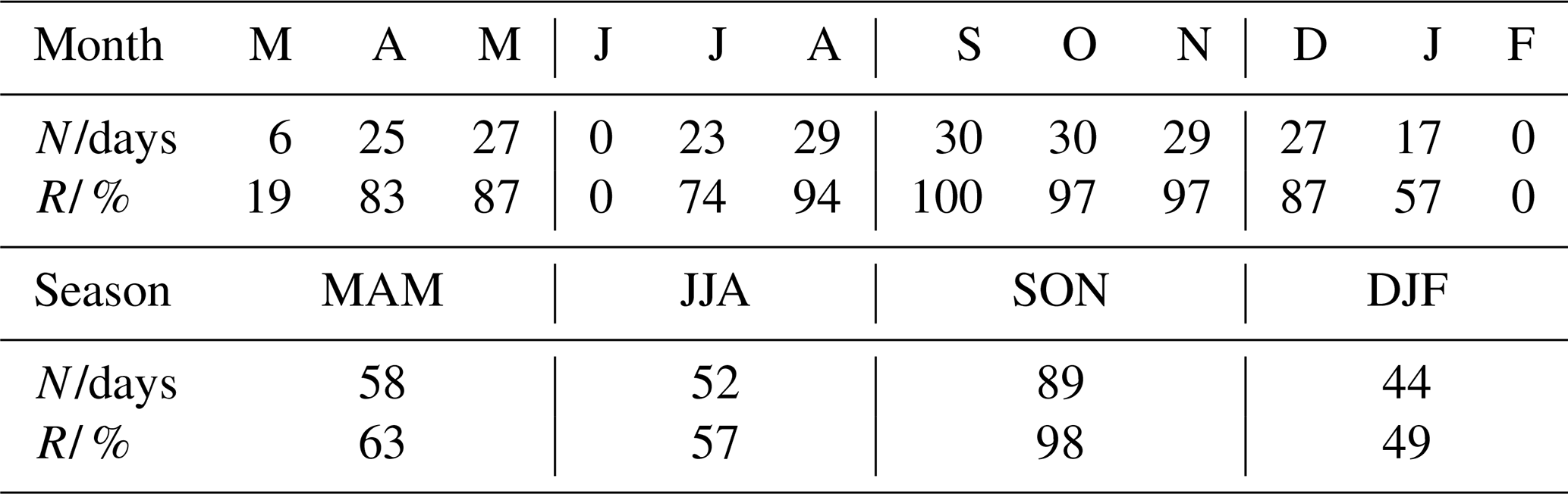
The instruments were equipped with battery backups to ensure controlled shutdown and recovery in case of a power shutdown. Nevertheless, this did not work in every case for every instrument and led to several missing days. An instrument failure of the cloud radar led to no data from the end of May to the beginning of July, and damage to the radar radome forced us to shut down the instrument on 22 January 2019. As the Cloudnet retrieval can only be applied when all instruments provide data, this led to 243 d of data or 72 % of the full year. Table 2 shows how many days are available per month. There are few or no days with data in March, June, and February and only 57 % in January.
Table 2Number of days when all instruments could provide data to the Cloudnet retrieval during every month and season. Months are indicated by their first letter, N is the number of days with data and R is the data coverage relative to the days in the respective month or season in percent.
2.3.2 Boundary-layer classification
In addition to the standard Cloudnet classification algorithm, we use the boundary-layer classification scheme described by Manninen et al. (2018), which is a Cloudnet add-on product. This scheme can identify the regions in the atmospheric boundary layer below the cloud with significant turbulence and determine the origin of this turbulence. The classification is provided as a function of time and height at a resolution of 3 min and 30 m. It is based on calculations of the turbulent dissipation rate from the Doppler lidar vertical velocities, the skewness of the vertical velocity distribution, the derived horizontal wind speeds and backscatter coefficients, as well as the near-surface temperature gradient around 2 m height.
At every height and at every time, six classes of turbulence origin are provided: in-cloud (if backscatter at a certain height is above a certain threshold), non-turbulent (a turbulent dissipation rate below a certain threshold), cloud-driven (skewness of the vertical velocity distribution is negative), convective (unstable stratification at the surface and turbulent conditions between the considered height and the surface), and wind-shear (wind shear above a certain threshold). If a turbulent layer is neither “cloud-driven”, nor “convective”, nor “wind-shear”, it is assigned “intermittent”. Additionally, the scheme provides information on whether the surface layer is stable or unstable.
3.1 Satellite view of a typical situation
A typical situation off the western coast of northern Chile is depicted in Fig. 2. The ocean on the left-hand side of the scenes is nearly completely covered by stratocumulus clouds, while the Atacama, the Andes, and the Altiplano to the right are nearly completely cloud-free as they are above 1000 m a.s.l. and thus higher than the MBL.

Figure 2Scenes of the visible GOES16 channel of the 30 August 2018 morning (12:00 UTC, top left), noon (17:00 UTC, top right) and afternoon (20:00 UTC, bottom left). The scenes are centered at 70∘ W and 21.9∘ S and cover about 800 km × 800 km. Three-letter codes indicate the locations of the airports of Arica (ARI), IQQ and Antofagasta (ANF). Plus signs indicate positions for which SST was extracted from GHRSST data (Naval Oceanographic Office, 2008). Digits 1–3 indicate locations of valleys cutting through the coastal mountain range. Thin black lines identify the coast or state boundaries, respectively. The large white area in the upper right corner of the satellite scenes is the salt pan Salar de Uyuni. The satellite scenes are courtesy of NASA Marshall Space Flight Center (https://weather.msfc.nasa.gov/goes/, last access: 6 September 2022).
The whole cloud deck typically moves along the coast to the north, turning gradually to the northwest as it approaches the Peruvian coast. This movement can be depicted by the two open-cell areas above the ocean which appear at different locations in the morning and noon images. From the displacement, we can estimate for these scenes a velocity of around 3 m s−1. Typical values go up to 7.5 m s−1.
In the morning scene, clouds reach inland at some places: to the northwest of Arica, around Antofagasta, especially at the Mejillones Peninsula at Antofagasta (ANF), and at the southern edge of the scene. All these locations lie at lower altitudes, and the edge of the stratocumulus identifies where the landscape reaches cloud-top height. At the coast, in the morning, there are some gaps in the cloud deck, some of which can be related to valleys cutting through the coastal mountain range. At these places dry desert air from the nocturnal flow from the Andes can probably reach the ocean and evaporate the clouds (see, e.g., Schween et al., 2020). Additionally, to the southeast of Iquique, a fog field can be seen inland in the central valley between the coastal mountain range and the slopes of the Andes (compare Cereceda et al., 2008b; del Rio et al., 2021a; Böhm et al., 2021).
At noon the situation has changed: at some places between Antofagasta and Iquique, larger gaps in the stratocumulus cloud deck opened and reached several tens of kilometers out over the ocean. This typical pattern can be observed nearly every day: between morning and noon these gaps form at the coast and during the day extend further over the ocean. In the afternoon, clouds form again at the coastal cliff and grow over the ocean. As a result, the gaps in the cloud deck are closed in the evening or early night, and a continuous stratocumulus cloud field extending from the open ocean to the coast is reestablished. Some sample plots and a discussion of this winter day and a summer day can be found in the Appendices A and B.
3.2 Wind
Over the seasons, average wind profiles at Iquique show a clear diurnal course (Fig. 3), with overall low wind speeds during nighttime and higher values during daytime, with the highest values in the afternoon below 200 m above the surface. During night, wind directions below 500 m are around southeast, with speeds of about 2 m s−1. Above 500 m one may observe northwesterly winds. After sunrise, wind direction in the lowest 500 m turns to the southwest and gradually increases to reach the highest average speeds of 7.5 m s−1 in the late afternoon (20:00 UTC = 2 h before sunset). At higher levels wind direction turns to the left, reaching south in the middle and east at the top of the observable layer. Wind speeds decrease in the evening and reach nighttime values again in the first half of the night.
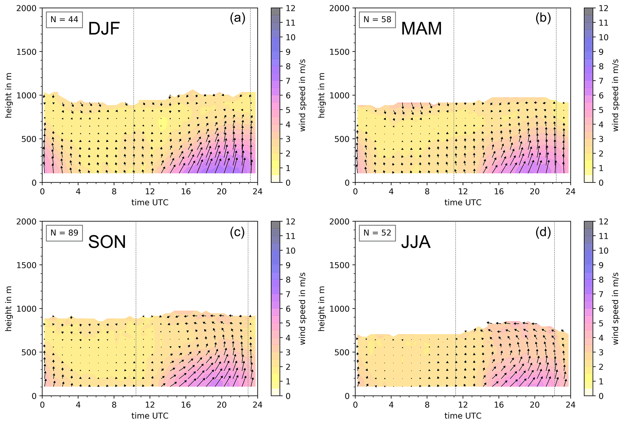
Figure 3Mean horizontal wind speed (shading, length of arrows) and wind direction (arrows) during different seasons as a function of time of day and height. Clockwise: (a) austral summer (DJF), (b) fall (MAM), (d) winter (JJA) and (c) spring (SON). The value of N gives the number of days analyzed. Vertical dashed lines indicate the average times of sunrise and sunset. Night appears on the left-hand side and day on the right-hand side of each plot.
Only a few details vary over the seasons. The range where a retrieval is possible is higher in summer and fall and low in winter. This is related to the presence of clouds mainly in winter and spring limiting retrieval height during these seasons. In summer, afternoon average speeds in the lowest 200 m reach 7.5 m s−1 but only 6.5 m s−1 or less during the other seasons. This can be related to two things: summer brings more insolation and, as we will see below, there are far fewer clouds in summer. Additionally, in summer, the center of the southeastern Pacific high-pressure system lies at the same latitude as Iquique and thus brings stronger winds.
The observed wind pattern resembles a land–sea breeze: during daytime a sea breeze is present, with inflow from the ocean to the land in the lower part of the MBL and a back circulation towards the ocean in the upper half. The back circulation is stronger in winter and spring when more clouds are present, while the sea breeze is stronger in summer, when insolation leads to a stronger temperature difference between land and sea. Superimposed on this is the southerly wind of the southeastern Pacific high-pressure system and the South American coastal jet (Muñoz and Garreaud, 2005), which due to channeling along the coastal cliff further increase daytime wind speeds. The land breeze during the night is much weaker because the temperature difference between cold ocean waters and the desert is small.
3.3 Temperature profile
We use the temperature profiles from the microwave radiometer to calculate the potential temperature with respect to the surface as with . This is not exact, but deviations are, below 900 m, typically well below 0.1 K. Average potential temperature θ shows some variation over seasons and time of the day (Fig. 4). In the middle of the MBL we see average potential temperatures between 15 (winter) and 21 ∘C (summer), respectively. In the free troposphere at 1.5 km height average potential temperature remains nearly constant at around 32 ∘C over the year. Nevertheless, there are some important features. The MBL is topped by a very strong inversion. Winter data from the radiosonde of Antofagasta, 320 km to the south, frequently show a temperature increase of around 10 K with maxima up to 17 K within less than 100 m. Although the MWR cannot resolve these extreme gradients, it clearly shows the inversion with a strong increase in θ with height, and we may regard the maximum of the gradient in this “radiometer inversion” as the true height of the MBL (see Sect. 2.2.2). It shows nearly no variation over the year and is lowest in winter at 950 m and around 1050 m during the other seasons. Despite the coarse resolution of the MWR, this agrees with the annual course of the median inversion base height for the period from 1979 to 2007 in Antofagasta shown by Muñoz et al. (2011). Nevertheless, we have to consider that cloud base, and thus probably also inversion height in Iquique, is on average about 180 m higher than in Antofagasta (Muñoz et al., 2016). Additionally, the inversion height data from the Antofagasta radiosonde (Muñoz et al., 2016) show, besides a weak decrease of −16 m per decade, a large year-to-year variability on the order of ±100 m. This makes it difficult to place our observations in relation to these long-term analyses. Over all seasons, MBL height shows no diurnal variation (Fig. 4). Similar temperatures above the inversion show no significant variation over the year.
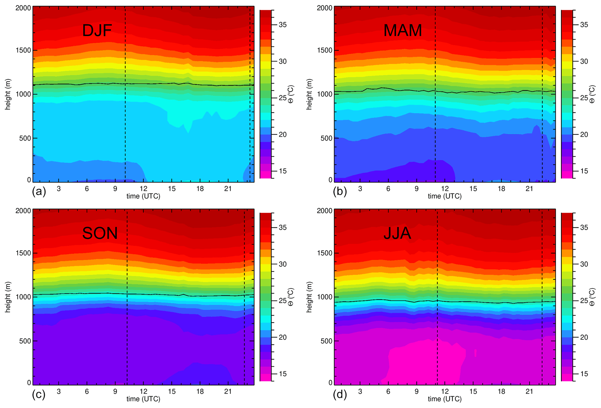
Figure 4Mean potential temperature during different seasons as a function of time of day and height. Clockwise: (a) austral summer (DJF), (b) fall (MAM), (d) winter (JJA) and (c) spring (SON). Color shading is based on 3-month averages of 1 h and 30 m intervals. Black line depicts the average height of the strongest gradient. Vertical dashed lines indicate average times of sunrise and sunset. The analysis here is restricted to the same days as the Cloudnet retrieval.
In summer and fall, close to the surface, values of θ are typically lower than at the bottom of the inversion; i.e., stratification is stable, in contrast to winter and spring, when it is neutral. This has strong implications for the presence of clouds as a stable stratification inhibits supply of water to the clouds. Lobos-Roco et al. (2018) have shown that, during stable stratification between their site at 1100 m a.s.l. and the airport at 53 m, typically no clouds are present. Accordingly we can expect that during the summer months fewer clouds will be present.
3.4 Cloud occurrence
The Cloudnet target classification scheme is used to investigate the FOC of warm clouds with cloud bases lower than 2 km a.s.l. (Fig. 5). Most clouds occur in winter and spring, when during the night about 90 % of the time clouds are present, while during summer and fall this decreases to 25 % and 45 %, respectively. During daytime FOC reduces by about 30 percent points compared to the night, meaning nearly no clouds during summer afternoons and somewhat more clouds in fall and spring. In winter FOC always stays above 60 %.
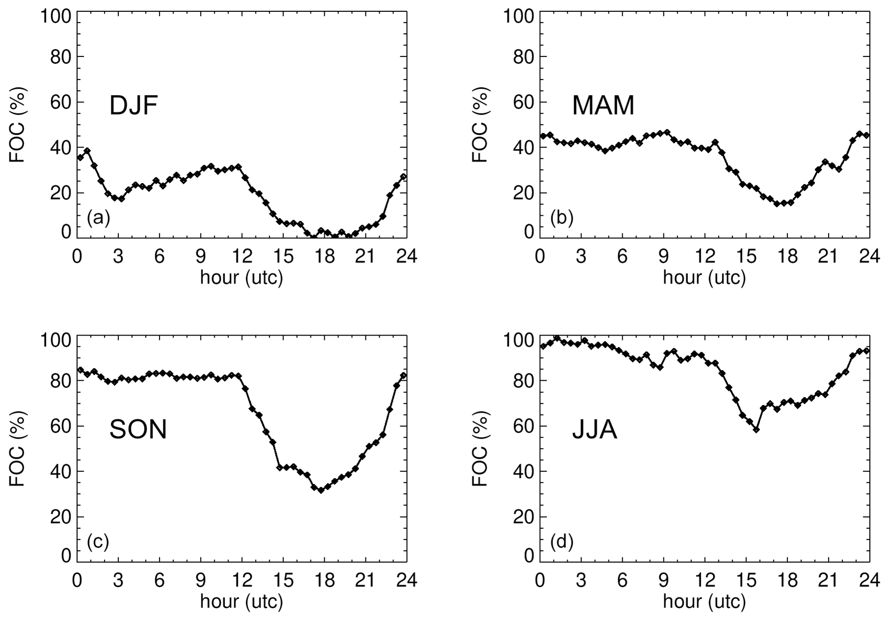
Figure 5Diurnal course of frequency of occurrence of clouds detected by Cloudnet with cloud base <2 km a.s.l. during different seasons. Clockwise: (a) austral summer (DJF), (b) fall (MAM), (d) winter (JJA) and (c) spring (SON). Vertical dashed lines indicate the average times of sunrise and sunset.

Figure 6Frequency of occurrence (FOC) of clouds with cloud base below 2 km a.s.l. in time × height bins during different seasons. Clockwise: (a) austral summer (DJF), (b) fall (MAM), (d) winter (JJA) and (c) spring (SON). The value of N gives the number of days analyzed. Vertical dashed lines indicate the average times of sunrise and sunset.
The vertical structure of the cloud varies as well (Fig. 6). In general, clouds can be found at higher levels in summer than in the other seasons, with the lowest clouds in winter. However, while in summer, and to some extent in fall, there is no clear cluster where we can expect clouds, during winter and spring they are clearly confined to a height range from 300 to 1100 m in winter and from 600 to 1200 m in spring. The diurnal course reveals that the reduction of cloud occurrence between noon and afternoon occurs from below. The lower boundary of the region where to expect clouds increases from morning hours to the afternoon by several hundreds of meters. This is in agreement with the observations of del Rio et al. (2021b) made some kilometers to the southeast at the slopes of the coastal mountains in another year.
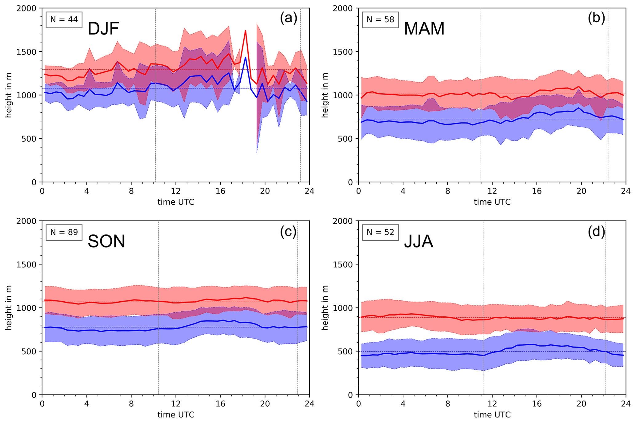
Figure 7Average diurnal course of the cloud base (blue) and cloud top (red) during different seasons. Clockwise: (a) austral summer (DJF), (b) fall (MAM), (d) winter (JJA) and (c) spring (SON). Color shading indicates the range of 1 standard deviation. The value of N gives the number of days analyzed. Vertical dashed lines indicate the average times of sunrise and sunset.
The same pattern can be observed if we investigate average cloud boundaries (Fig. 7). Over the whole day, the average cloud top is at about the same height: 1000 m in fall, 1100 m in spring, and 900 m in winter. In contrast to this, the cloud base is lowest during the night and increases from sunrise until afternoon by about 50 (spring) to 100 m (fall and winter). An exception to this pattern occurs in summer, when the cloud base as well as cloud thickness increase over the day, which is more typical for shallow cumulus clouds. Nevertheless, cloud occurrence in summer is low, and the variability of the cloud boundaries is larger than cloud thickness, such that these numbers should be interpreted carefully. Nighttime cloud bases are highest in summer (around 1100 m), intermediate in fall and spring (700–800 m), and lowest in winter (500 m). Cloud thickness is about 300 m during fall and spring and 400 m in winter nights. Muñoz et al. (2016) found in a 33-year dataset from Iquqique, centered around 1997, a similar pattern with cloud bases higher during the day than during the night. Nevertheless, they found lower night-to-day amplitudes (50–75 m) and also cloud bases which were, especially in fall and winter, about 200–300 m higher then we observed now. This difference can only partly be explained by the trend of −100 m for every 15 years that they found. From this comparison it seems as if this trend has accelerated.
The diurnal course with a constant cloud top and a rising cloud base during daytime indicates that processes within the MBL are the reason for the observed thinning of the cloud deck during daytime. A possible mechanism to explain this could be the absorption of solar radiation during daytime, so that longwave radiative cooling at the cloud top is largely cancelled out and the formation of subsiding turbulent eddies at the cloud top is inhibited. As a result, the sub-cloud layer is not well-mixed, vertical moisture transport from the ocean is at least reduced, water loss by detrainment and thus evaporation into the free troposphere at the cloud top is not compensated anymore, and the MBL becomes drier. A lower water vapor content means a higher cloud base or even no cloud (Bretherton et al., 2004). However, this cannot explain why the cloud deck starts to evaporate at the coast. Another mechanism could be the general circulation pattern at the coast in which air flows over land. While flowing over warm solid ground, air heats up, which increases the lifting condensation level. This could explain why clouds evaporate especially at the coast.
3.5 Liquid water path
As discussed above (Sect. 2.2.2), we use four different retrievals based on different pre-processing of the radiosonde data to derive the LWP (Fig. 8). The average difference between the resulting values is small (3 g m−2) but shows a diurnal course with larger values during the night (up to 18 g m−2). The theoretical retrieval uncertainty of the LWP is determined as 10 g m−2. Calibration and absorption model uncertainties can lead to systematic LWP offsets which can amount to a maximum error of 20–30 g m−2. These effects have been corrected for by applying a clear-sky offset correction, which is applied to all-sky observations. Thus, we expect a random uncertainty for individual values of not significantly more than 10 g m−2, which further reduces for seasonal averages by a factor of . That is, LWP uncertainty is dominated by the uncertainty of the radiosonde data preprocessing.
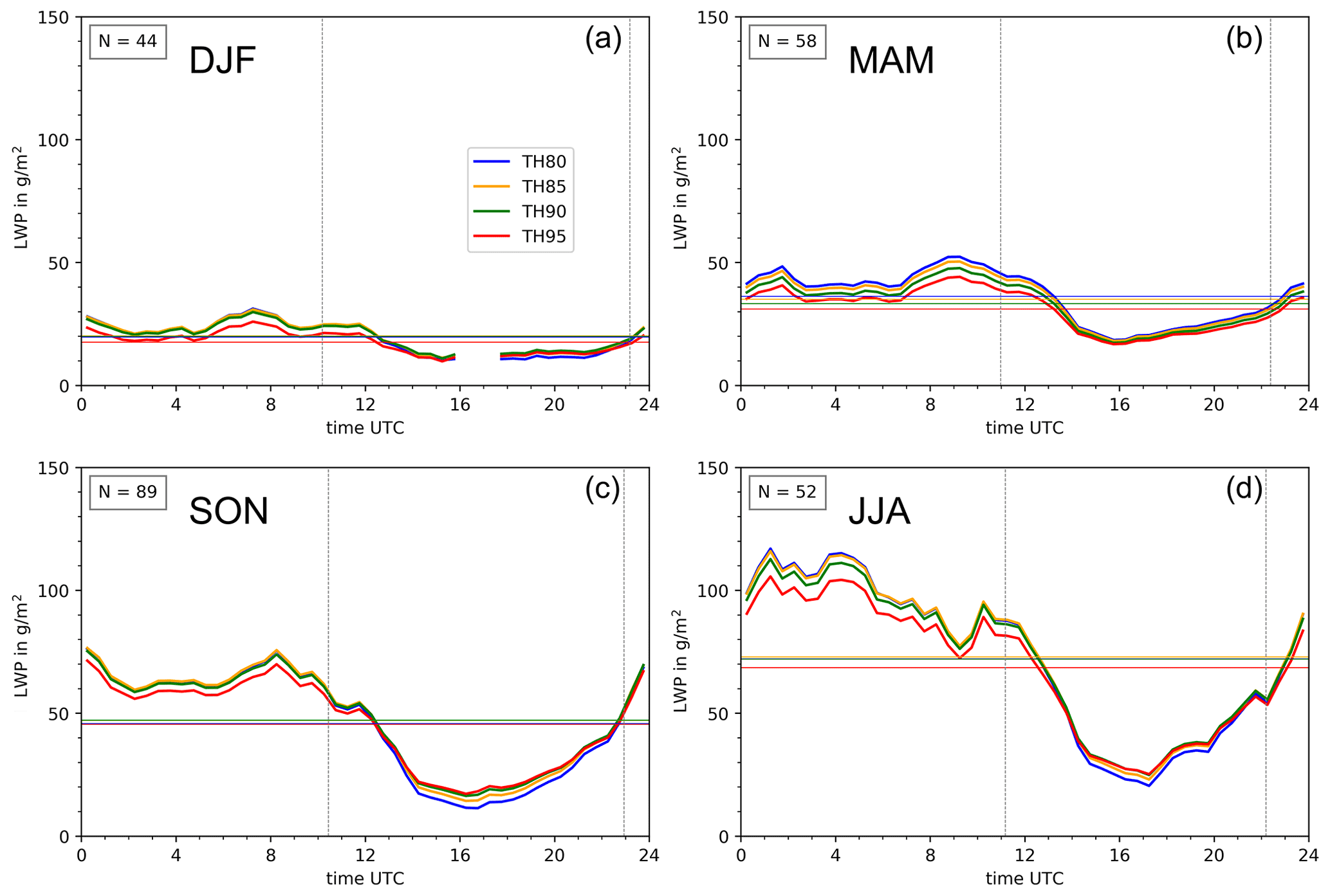
Figure 8Average diurnal course of the liquid water path (LWP) during different seasons. Clockwise: (a) austral summer (DJF), (b) fall (MAM), (d) winter (JJA) and (c) spring (SON). Different colors depict different LWP retrievals (see Sect. 2.2.2). Horizontal lines indicate seasonal averages. The value of N gives the number of days analyzed. Vertical dashed lines indicate the average times of sunrise and sunset. The gap around 17:00 UTC in austral summer (DJF) is due to times when the Sun is in zenith, making retrieval impossible.
In general, the average LWP is lowest in summer (average value 20 g m−2) and highest in winter (70 g m−2) (Figs. 8 and 9). Diurnal courses show a recurring pattern with maximum values during the night and a minimum in the early afternoon. Daily amplitudes are largest in winter (70 g m−2), smaller in fall and spring (25 and 50 g m−2), and nearly negligible in summer (17 g m−2). The diurnal amplitude in winter and spring equals the average values, i.e., the clouds lose half of their water on average during daytime. The standard deviation of the half-hourly averages of the diurnal courses, i.e., day-to-day variability for the respective hours, is on the order of the average values themselves (not shown). It is noteworthy that in winter (JJA) the maximum LWP is found in the first half of the night and that values decrease thereafter. This might be explained by the occurrence of drizzle, especially in the nights of August, when up to 40 % of the time drizzle occurs. Drizzle removes liquid water from the cloud when it falls out of the cloud. While nighttime average values in spring (60 g m−2) are significantly lower than those reported by Bretherton et al. (2004) for the open ocean in October (100–220 g m−2), they agree well with those reported for the Chilean coast (Mechoso et al., 2014).
3.6 Drizzle
Drizzle plays an important role in the moisture budget of stratocumulus clouds (Wood, 2012), and it may also be an additional water supply to the coastal mountains and their fog oases. We therefore investigate here how often drizzle occurs and how far down it reaches. The Cloudnet classification scheme provides two classes, “drizzle or rain” and “drizzle or rain coexisting with cloud liquid droplets”. As the weather station never detected rain, we assume that these classes always identify drizzle, and we can investigate at which times and heights drizzle occurs below and within the stratocumulus. We consider all cases with drizzle and a cloud present below 2 km and count all cases with drizzle in every hour over the whole year and additionally in every month over all hours. We use these numbers to calculate the relative amount of time or frequency of occurrence of drizzle per month and per hour. We also identify the lowest level that drizzle reaches. During the whole observation period, drizzle evaporated on average at 485 m and reached only sporadically the lowest Cloudnet level of 200 m. Regarding monthly averages, the lowest average height where drizzle occurred was in June and July at 300 m above ground, while on a hourly basis over the whole year the lowest average drizzle base was 450 m during the night. Nevertheless, it should be noted that drizzle may reach the ground further inland, where altitudes increase quickly with distance to the coast. The height zde at which drizzle evaporated completely showed some dependence on the cloud base and cloud top: the higher the cloud base and top, the higher the zde, with thicker clouds leading to lower zde (Fig. 10a).
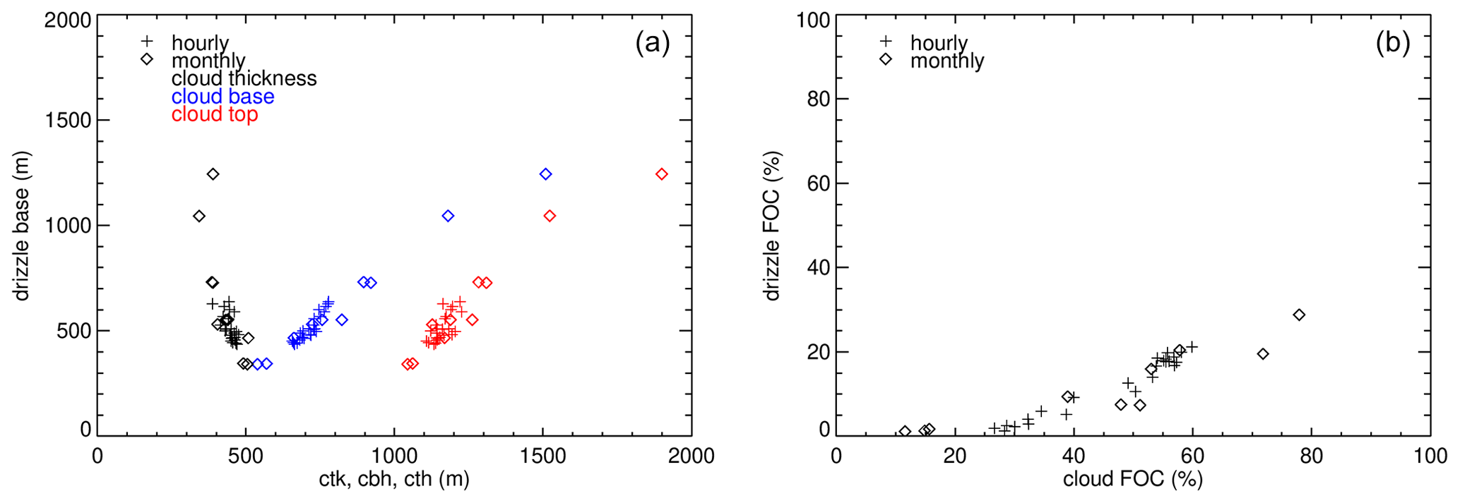
Figure 10(a) Drizzle basis (height at which drizzle evaporates completely zde) as a function of the cloud base (blue), cloud top (red), and cloud thickness (black). (b) FOC of drizzle at any height as a function of FOC for clouds. Monthly averages over all hours are denoted by a + symbol, and hourly averages over all months for different hours are indicated by a ⋄ symbol.
The frequency of occurrence of drizzle follows that of clouds, with a difference of 30 to 40 percent points (Fig. 10b). This is observed in the monthly averages as well in the diurnal course, where most of the drizzle occurs during the night, on average 20 % of the time reaching up to 47 % in the nights of August (not shown).
3.7 Turbulence
The mean standard deviation of vertical velocity (σw, Fig. 11) remains most of the time below 0.5 m s−1. Only during daytime do higher values develop from the ground and reach up to 300 m in summer and fall and 750 m in winter and spring. During nighttime the upper half of the MBL shows, especially in winter and spring, slightly higher values.
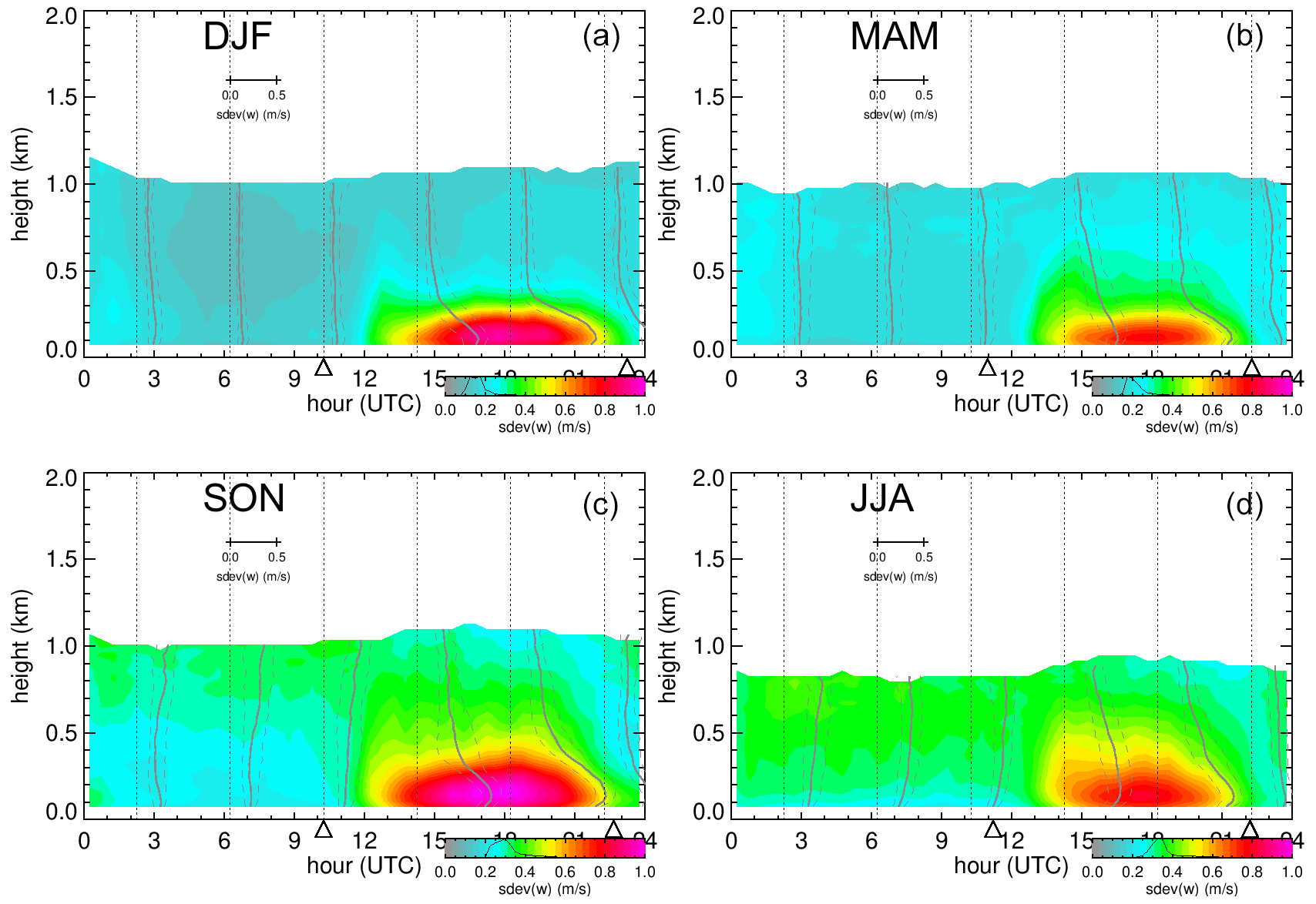
Figure 11Time–height sections of the mean standard deviation of vertical velocity (color shading, calculated as described in Schween et al., 2014) for, clockwise, (a) summer (DJF), (b) fall (MAM), (d) winter (JJA) and (c) spring (SON). Gray lines are the median profiles (solid) and interquartile range (dashed) at the times indicated by the dotted vertical lines. Time is given in hours UTC such that night appears on the left-hand side and daytime on the right-hand side of each plot. Triangles at the abscissa indicate average times of sunrise and sunset, respectively.
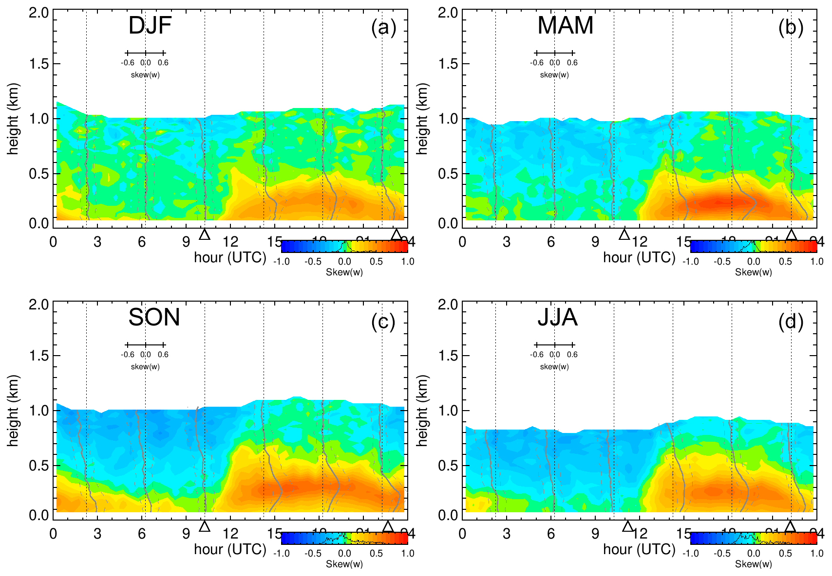
Figure 12Time–height sections of vertical velocity skewness during the four seasons (color shading). Gray lines are the median profiles (solid) and interquartile range (dashed) at the times indicated by the dotted vertical lines. Time is given in hours UTC such that night appears on the left-hand side and daytime on the right-hand side of each plot. Triangles at the abscissa indicate average times of sunrise and sunset, respectively.
The mean diurnal course of the skewness (Fig. 12) shows distinct night and day patterns. During the night skewness is mostly negative, with the lowest values in the upper half of the MBL, while during daytime skewness in the lower two-thirds of the MBL is clearly positive. Nighttime skewness is most negative in winter and spring. Daytime positive skewness reaches higher up in winter and spring than in summer and fall. Most positive skewness occurs at heights in the range 200–300 m.
Vertical velocity in rising as well as subsiding plumes is typically concentrated in narrow chimneys with high speeds surrounded by larger regions with only small velocities compensating for the mass transport in the plume cores. As a result, regions with rising plumes show positive skewness, and regions with subsiding plumes show negative skewness. Accordingly, nighttime turbulence is driven mainly by subsiding plumes, and daytime turbulence is driven by plumes rising from the surface. Nighttime as well as daytime turbulence in winter and spring is more intense and reaches further down and further up, respectively, when compared to the other half of the year.

Figure 13Diurnal course of FOC of boundary-layer classes during different seasons. Clockwise from panel (a): austral summer (DJF), fall (MAM), winter (JJA) and spring (SON). The value of N gives the number of days analyzed.
To further investigate how frequently which type of turbulence occurs and how far its influence reaches, we use the boundary-layer classification scheme of Manninen et al. (2018). We are mainly interested in whether there is turbulence and whether this turbulence is connected to the cloud (“cloud-driven”), the surface (“convective”), or wind shear or whether its source cannot be identified (“intermittent”). Whereas in summer and fall a significant amount of the time (45 %–65 %) is classified as non-turbulent, winter and spring show far fewer calm moments (5 %–35 %; see Fig. 13). Convective turbulence is present during daytime in all seasons when stratification at the surface is unstable but is most frequent in winter and fall (up to 65 %). The same is true for cloud-driven turbulence, which occurs most frequently in winter nights (20 %), while it is nearly not detected in summer and rarely in fall (8 %).
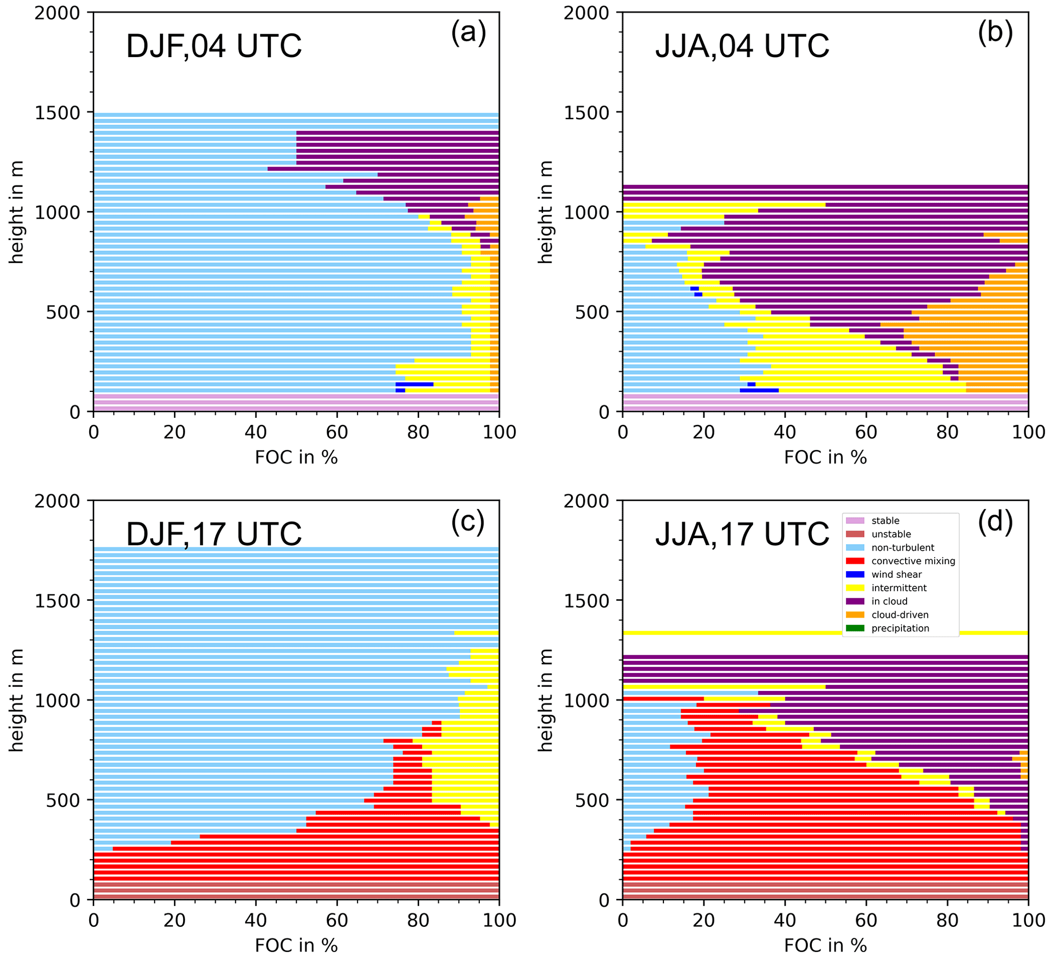
Figure 14Frequency of occurrence of boundary-layer classes at different heights in austral summer (DJF, a, c) and winter (JJA, b, d) around local midnight (04:00 UTC = 00:00 LT, a, b) and early afternoon (17:00 UTC = 13:00 LT, c, d).
The vertical distribution of turbulence classes reveals that, although rarely occurring, in summer nights cloud-driven turbulent mixing may nearly always reach down to the surface (Fig. 14). In winter nights cloud-driven turbulence occurs much more frequently (30 % at average cloud-base height), but its frequency decreases from the cloud base towards the surface by about one-third. Given the typically low winds during the night and thus the lack of other possible sources of turbulence, one might speculate that the origin of “intermittent” turbulence during the night is also due to the clouds, although vertical velocity does not show negative skewness. This would increase the frequency of cloud-driven turbulence and remove the height dependence. Under this assumption turbulence originating from the clouds reaches the surface in every case and thus mediates the transport of moisture from the ocean into the MBL.
During daytime at local noon, turbulence is mainly convective; i.e., it is driven by heating of the ground. However, while in summer it stays mostly confined to the lowest 500 m above the ground and well below the average cloud base at 1100 m, in winter it can reach up to 1000 m and is typically connected to a cloud. This seasonal difference in convective turbulence reflects the different stratifications during the two seasons.
To be able to interpret the observations, we first review the mechanisms which maintain the marine stratocumulus (see, e.g., Wood, 2012). Based on this and the observations described so far, we then try to give a holistic picture of the seasonal and daily stratocumulus situations at the northern coast of Chile.
Tropical stratocumulus clouds are typically capped by a strong inversion and a very dry layer above. They continuously lose water by evaporation to the dry, free troposphere. As they exist permanently over large regions, effective mechanisms must exist to balance this water loss. Especially during night, the difference of longwave radiation emitted by the stratocumulus cloud top and the low downward emission of the dry atmosphere above leads to significant radiative cooling at the cloud top. Evaporative and radiative cooling at the cloud top generates pockets of cold air that organize into plumes of cold air that subside towards the ocean surface. The movement of the descending plumes in the stratocumulus-capped MBL is compensated by ascending air, these interchanging upward and downward movements generating a well-mixed layer. This is similar to a convective boundary layer (CBL), where plumes with positive buoyancy are generated at the warm surface and ascend through the whole boundary layer, leading to intensive mixing and neutral stratification. The stratocumulus-capped maritime boundary layer (SCBL) can thus be seen as an “upside-down convective boundary layer” with similar mechanisms. Comparable to a CBL, intense turbulent mixing in the SCBL leads to neutral and moist–neutral stratification below the cloud and in the cloud, respectively, and like the CBL, which warms up as a whole, the SCBL cools as a whole until it approaches SST at its bottom, and similarly to convective plumes, which due to their inertia can reach up into the inversion at the CBL top and mix warm air into the CBL, cold air plumes in a SCBL can reach through a sufficiently thin stable layer at the sea surface. In this case descending plumes can reach the ocean surface and moisture from the ocean surface is mixed upwards to the cloud and thus can compensate for the moisture loss to the free troposphere. In contrast to this, a stable stratification over large ranges of the SCBL would inhibit the replenishment of water to the cloud, as it inhibits the descent of plumes to the sea surface.
As long as the SCBL is well mixed and in a stable state, cloud-top energy and mass fluxes must be compensated by fluxes at its bottom. If these fluxes are not balanced, the SCBL will change its temperature and/or water content. Radiative emission at the cloud top must be balanced by sensible heat flux from the ocean surface. Loss of water vapor by detrainment into the free troposphere must be compensated by evaporation at the ocean surface. Drizzle removes liquid water from the cloud. However, as long as it does not reach the surface, it does not change the water content of the MBL. A further factor is large-scale subsidence. In a CBL warm rising plumes cross the inversion and thus lead to a growth of BL height, and this growth is reduced by subsidence (see, e.g., Ouwersloot and Vila-Guerau de Arellano, 2013). In a SCBL this role of resistance against subsidence is taken by the entrainment of air from above the BL (Wood, 2012). Nevertheless, entrainment rates remain a factor of uncertainty.
4.1 SST and seasonal forcing
To investigate the relation of the MBL temperature to SST in our dataset, we calculate the potential temperature θs with sea surface as the reference level. We use θs at 0.3 km derived from the MWR measurements as a measure for θs in the whole MBL and θs at 1.5 km as a measure for the free troposphere temperature.
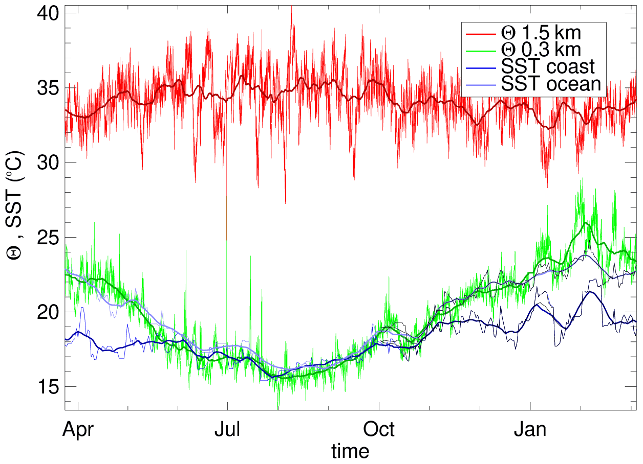
Figure 15Air and ocean temperatures from April 2018 to March 2019 with potential temperature with reference pressure at sea level (Θ) from MWR measurements for 1.5 (red) and 0.3 km (green) height and sea surface temperature (SST) 5 km from the coast (light blue) and 50 km to the southwest in the open ocean (dark blue). Thin lines indicate 15 min (Θ) or daily (SST) values, whereas thick lines are 30 d gliding averages.
We provide SST from two points: one from 5 km west of the Iquique site which is representative for the temperatures of coastal waters, and a second point in the open ocean 50 km to the southwest. The open-ocean point has been chosen with the idea that air arriving at Iquique with wind speeds between 2 and 7 m s−1 from the southwest has passed this point between 2 and 7 h before, respectively. The SST close to the coast at Iquique shows an annual cycle with a minimum in August (15.5 ∘C) and a maximum in February (21 ∘C; see Fig. 15). The open-ocean SST shows a larger amplitude with summer maxima above 25 ∘C, whereas in winter it can go down to below 15 ∘C. This larger amplitude is due to variations in the location of the Humboldt Current. As can be inferred from the global SST datasets (Naval Oceanographic Office, 2008, 2018), at some point the Humboldt Current turns to the northwest before it reaches the coast of Peru. In summer this turn occurs further to the south, and warmer waters propagate from the north along the coast of the continent. Nevertheless, upwelling still leads to a strip of colder waters direct at the coast of roughly 50 km width.
Our observations show that, from June to the beginning of November, the MBL at the coast has the same temperature as the ocean surface and is thus in equilibrium with the underlying ocean. During the remaining months between the middle of November and May, the MBL is warmer than the coastal ocean and thus decoupled from it. It is instead in equilibrium with the warmer waters 50 km off the coast and has been advected by the mean wind to the colder coastal waters. Temperature in the free troposphere at 1.5 km height shows only a weak annual variation which is smaller than the day-to-day variability. As a result, the temperature difference between the free troposphere and MBL is large in winter and small in summer (Figs. 4 and 15). A strong temperature difference or strong inversion decouples the MBL from the free troposphere and thus inhibits the loss of moisture to the free troposphere.
When the MBL has the same temperature as the ocean, plumes from cloud top can reach the ocean surface, and moisture from the ocean is mixed into the boundary layer and the cloud layer. In winter we have accordingly two mechanisms which support a persistent thick stratocumulus cloud deck: coupling of the MBL to the ocean surface and decoupling of the MBL from the free troposphere by a strong inversion. These winter conditions are accompanied by stronger large-scale subsidence caused by the then closer located center of the southeastern Pacific high-pressure system. This subsidence further sharpens the inversion and slightly lowers its height (Fig. 4) compared to summer. As a result, the winter season coincides with times of the most frequent cloud presence (Sect. 3.4, Fig. 6). In contrast, summer conditions are less favorable for a persistent stratocumulus: large-scale subsidence is smaller, and accordingly the inversion is less sharp and lies slightly higher. The weaker inversion allows a larger moisture loss to the free troposphere, whereas the stable stratification of the coastal MBL reduces the moisture supply from the ocean.
We believe that our 1-year data show that it is not only the absolute value of the SST at the coast, but instead its spatial variability and the advection of air from warmer to colder waters which influence the occurrence of the stratocumulus cloud. Accordingly, the interplay of the dynamics of the Humboldt Current, atmospheric advection, and coastal ocean upwelling as well as the large-scale subsidence is essential for the existence of stratocumulus clouds at the coast of the Atacama.
4.2 Local circulation and diurnal variation
We observed frequently that the stratocumulus cloud deck at the coast evaporates around noon and reappears in the afternoon or evening. The clouds evaporate from the bottom; i.e., cloud-base height increases, while cloud-top height remains constant (Fig. 7).
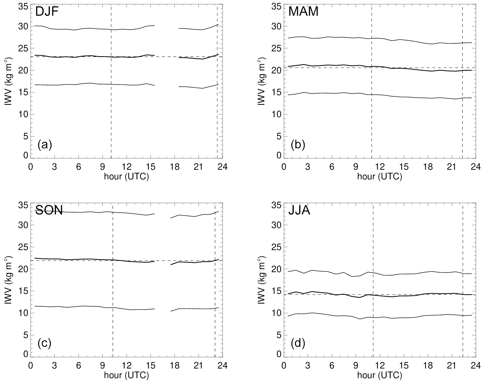
Figure 16Average diurnal course of column integrated water vapor (IWV) during different seasons (thick line) plus or minus its standard deviation (thin lines) as a measure for day-to-day variability. Clockwise: (a) austral summer (DJF), (b) fall (MAM), (d) winter (JJA) and (c) spring (SON). Vertical dashed lines indicate the average times of sunrise and sunset. The gap around 17:00 UTC in austral summer (DJF) is due to times when the Sun is in zenith, making retrieval impossible.
A rise of cloud base may have two reasons: decrease in water content or rise in temperature in the MBL. A decrease in water content could be explained via multiple steps: absorption of solar radiation by the cloud during daytime reduces cooling at the cloud top, and as a result, the formation of plumes, responsible for the mixing in the MBL, would be weakened. This mechanism has been observed by Bretherton et al. (2004) above the open ocean. In the MWR data a weak reduction of the column IWV at the time of the onset of the sea breeze on the order of 0.5 kg m−2 (Fig. 16) is observed in all seasons. This is only a small part of the IWV but a large amount compared to the LWP values, which lie in the range 0.01–0.1 kg m−2 (Fig. 8). Especially in winter and spring the IWV recovers around 17:00–18:00 UTC. This coincides with the time when clouds form again. Nevertheless, day-to-day variability of IWV at every hour is large, and these diurnal variations might just be random. Additionally, it must be noted that IWV is the column integrated water vapor, which means that entrainment of dry air from the free troposphere does not change the IWV.
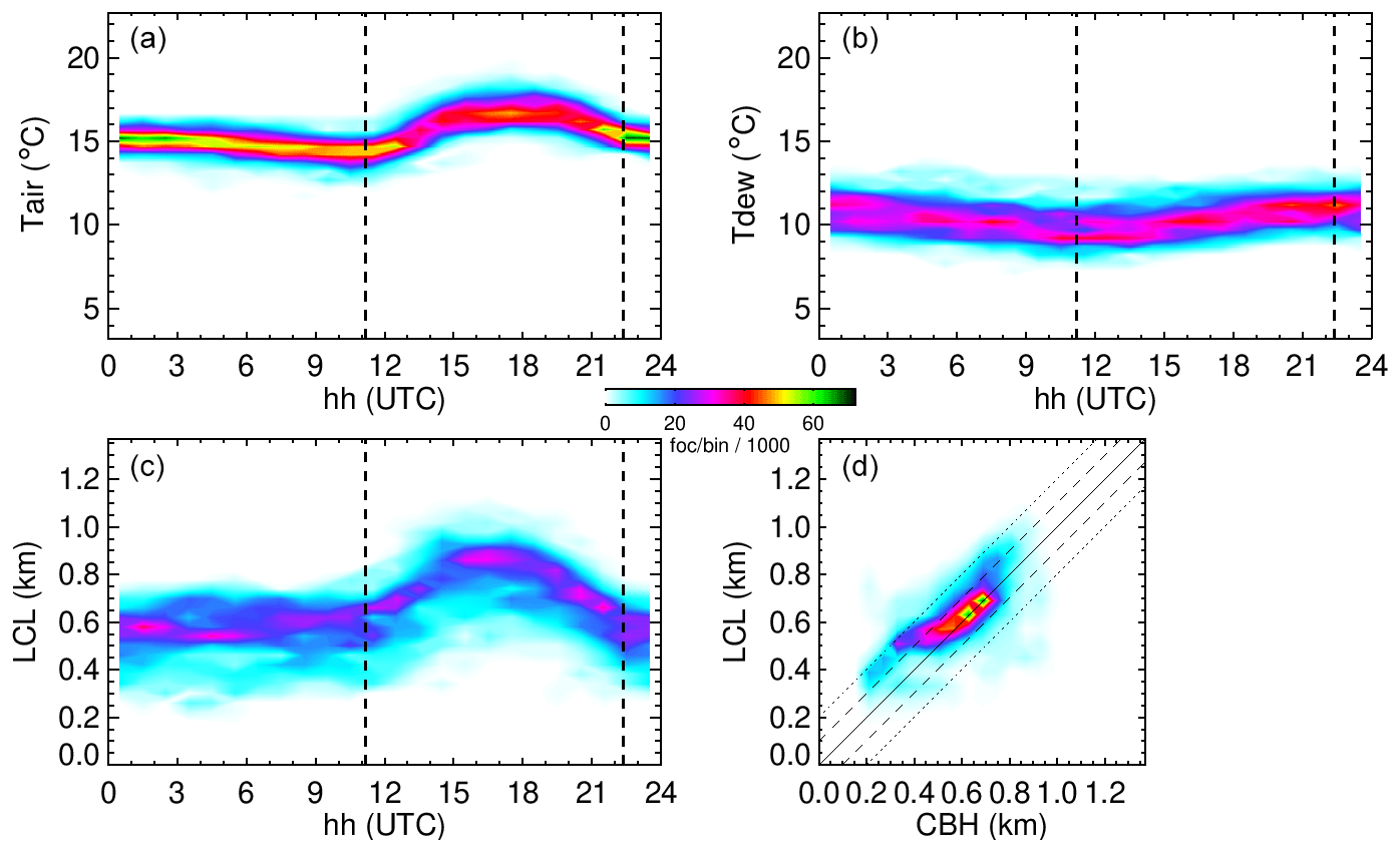
Figure 17Air temperature at 2 m (a), dew point (b), and lifting condensation level (LCL, c) versus hour and LCL versus cloud-base heights from Cloudnet (CBHs, d). All quantities during winter (JJA), presented as two-dimensional frequency distributions. Vertical dashed lines indicate the average times of sunrise and sunset, respectively. Diagonal lines in (d) indicate ±100 (dashed) and ±200 m (dotted) deviations from perfect agreement.
As the MBL is, especially in winter, well-mixed and neutrally stratified (Fig. 4), we can use 2 m temperature and humidity measurements to investigate the state of the MBL (Fig. 17) and lifting condensation level (LCL) to estimate cloud-base height. As a measure of the moisture content, we use the dew point. LCL is calculated by the linear estimate LCL=125 m K of Lawrence (2005), which is within ±12 m of the exact formula of Romps (2017) for the observed temperature and humidity range. Air temperature shows a typical diurnal course with low temperatures during night, an increase from the early morning hours, and a maximum at 18:00 UTC, i.e., in the early afternoon, which means that it is mainly defined by the radiative forcing by the sun. During the night and early morning, moisture, represented by the dew point, shows a decrease towards a minimum at about 12:00 UTC, after which it starts to increase. This increase coincides with the onset of the sea breeze around 12:00 UTC (see Fig. 3) and has its maximum rather late at 21:00 UTC, 2 h after the maximum of the sea breeze and 3 h after the air temperature maximum. Thus, at the surface, we observe mainly a change between dry desert and moist ocean air which is similar to observations in the coastal mountains (García et al., 2021) but also from other coastal stations (see the data described in Schween et al., 2020).
The resulting LCL is constant during night, increases from sunrise until a maximum at around 16:30 UTC, i.e., local noon, and decreases again until sunset. It accordingly follows the course of air temperature in the morning hours but decreases earlier in the afternoon. The reason for this afternoon behavior is the increased moisture content which allows the reformation of clouds in the afternoon.
Intercomparison between LCL and Cloudnet cloud-base height (CBH, Fig. 17d) shows some cases with LCL < CBH, a strong cluster between 500 and 700 m with LCL ≃ CBH which coincides with daytime heights of LCL. However, additionally there are several cases with LCL by up to 200 m higher than CBH. Especially for CBH below 500 m there appears a cluster with CBH of 100–200 m lower than LCL. This is not possible in a mixed BL, and even in a stratified BL it would require strong vertical humidity gradients.
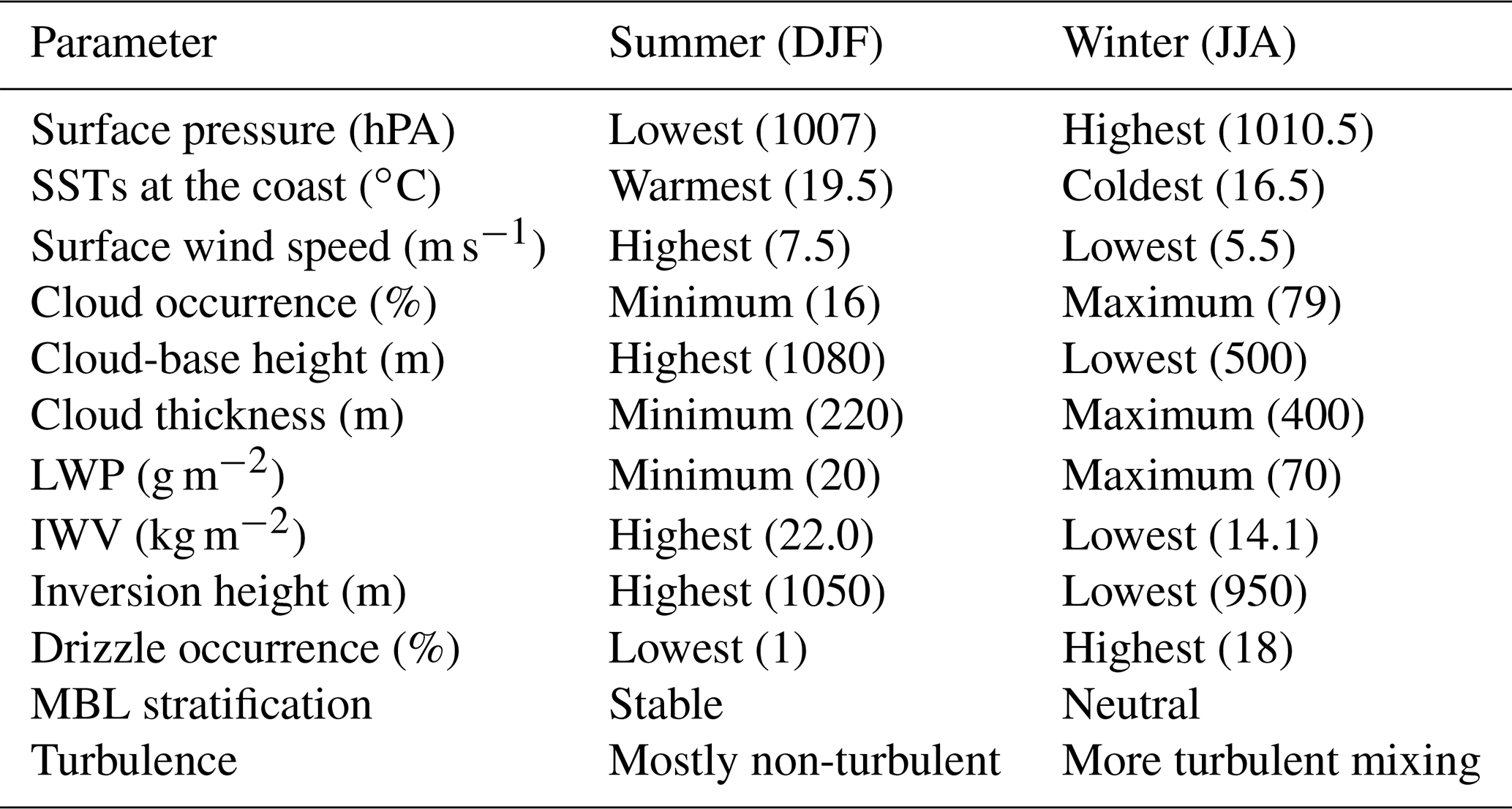
Table 3Summary of the major findings of the present work during the Iquique Airport observations (2018/2019) for austral winter (JJA) and summer (DJF). Values represent seasonal averages.
The airport has operated a ceilometer since 2017 (Vaisala CL31; see Direccion Meteorologica de Chile Servicios Climaticos, 2022; del Rio et al., 2021b). A ceilometer provides a “ceiling”, i.e., the largest height from which a pilot could see the earth's surface, and Vaisala ceilometers especially do so by estimating visibility for a pilot using several assumptions (Martucci et al., 2010). In contrast to this, the CBH retrieval of Cloudnet (and some other ceilometer manufacturers) is based on the fact that cloud droplets show strong backscatter. CBH is then identified by a combination of the values of the backscatter coefficient β and the occurrence of a strong vertical gradient in β (for details of the Cloudnet CBH algorithm, see Tuononen et al., 2019). As visibility decreases only above the cloud base, the ceiling is typically larger than CBH, with differences strongly depending on the cloud and cloud droplet properties (Martucci et al., 2010).
We compared CBH from the airport ceilometer to Cloudnet and saw a systematic underestimation by Cloudnet, especially during winter and night, with average differences around 100 m. Investigation of time series revealed that these large differences coincide with drizzle, especially during the night and morning hours. On the one hand, this might be due to the fact that it is difficult to differentiate between drizzle and cloud droplets in the backscatter signal, especially as drizzle originates from within the cloud (Tuononen et al., 2019). As a result, CBH may indeed become too low. On the other hand, drizzle increases humidity below the cloud and thus may lower the cloud base. In this case LCL based on surface measurements is not valid for an estimation of the cloud base any more.
With this information we can describe the diurnal life cycle as follows. In the morning hours, warming of the air from the surface evaporates the stratocumulus from the bottom. The upper branch of the sea-breeze circulation transports the warm, cloud-free air over the ocean and generates a cloud gap growing from the coast, as can be observed nearly every day in satellite images. With its onset, the surface branch of the sea breeze transports moist air towards the coast and therefore allows the reformation of clouds already in the afternoon, although temperature is then around its maximum. The upper branch of the sea breeze pushes these clouds over the ocean. Eventually the coastal cloud connects to the maritime stratocumulus deck, and after sunrise the process begins again.
We note here that the interaction of the land–sea breeze with the “Rutllant cell” as described in Rutllant et al. (2003) cannot be inferred from the wind lidar measurements as the latter is restricted to the aerosol-loaded MBL. The Rutllant cell comprises strong winds inland at altitudes around 1000 m a.s.l. and moisture transport into the hyperarid Atacama Desert (Schween et al., 2020). If the cell would extend over the ocean, strong wind shear would occur at the top of the MBL and could provide moisture from the MBL to the desert.
This paper presents ground-based remote sensing profiling observations of coastal stratocumulus clouds at the airport of Iquique at the northern coast of Chile. These clouds are a vital moisture supply for flora and fauna in the western part of the Atacama Desert.
The performed observations, for the first time, bring forth a full seasonal cycle of vertically resolved insights into the physical processes of the marine stratocumulus clouds interacting with the topography of northwestern Chile. The observations resolve the cloud vertical structure, including cloud classification and microphysics, the turbulent structure of the atmospheric boundary layer, as well as the temperature. Additionally, vertically integrated values of liquid water and water vapor have been recorded – all with a temporal resolution of seconds to minutes.
Clear seasonal and diurnal dependencies of cloud occurrence, geometrical extent, as well as liquid water content have been observed (see Table 3). Compared to austral summer, stratocumulus clouds in austral winter occur 4.9 times more often and are 83 % thicker (with 50 g m−2 or 3.5 times more LWP), while the cloud base is 580 m lower. These differences are strongly related to the seasonal SST patterns off the Atacama coast.
The diurnal cycle shows a distinct pattern with minimum cloud occurrence (with the lowest LWP) around 16:00 UTC and maximum occurrence (with the highest LWP) during night. Our observations show that at night clouds are maintained through turbulence originating from the cloud which connects them to the ocean surface. During daytime convective turbulence driven by the warm land surface frequently evaporates the stratocumulus cloud from the bottom. Clouds reestablish in the early afternoon as moister air is advected by the sea breeze. The upper branch of the sea-breeze circulation drives these clouds over the ocean.
During summer and fall, stratification in the MBL is typically stable, while winter and spring show neutral stratification and a well-mixed MBL. This somewhat counterintuitive behavior results from the SST distribution in the ocean: while in winter water temperatures are constant over a wide range of distances, summer is characterized by coastal water temperatures 5 K lower than 50 km and more from the coast. The driver of this difference is a farther westward position of the Humboldt Current. This allows warmer tropical waters to reach farther south during these seasons, while coastal upwelling maintains a low SST along the coast. The MBL appears to be in equilibrium with these warmer waters and becomes stably stratified when advected towards the coast, which, in turn, makes clouds less likely to persist.
Especially in spring, cloud cover at the northern coast of Chile seems weakly connected to El Niño ONI 3.4, i.e., the SST anomaly in the equatorial Pacific several thousand kilometers to the northwest (del Rio et al., 2021a). Our observations may help to understand the details of this coupling and allow predictions of future and past occurrences of stratocumulus clouds at the coast. Based on our observations, it will be possible to investigate details of the processes by use of large-eddy simulation (LES).
Figures A1–A3 show example data from all three instruments and the Cloudnet retrieval for 30 August 2018, a typical winter day with continuous cloud cover during most of the time, a cloud gap around noon, and drizzle during the night.
Wind profiles (Fig. A1) show during daytime strong southwesterly winds at heights below about 500 m and above a continuous turn to southeasterly and easterly winds. During the night wind changes between southwest and southeast, which may represent circulations induced by the falling drizzle. High attenuated backscatter β between 500 and 800 m identifies the lower part of the cloud. Inside the cloud the signal decreases due to extinction and a wind retrieval is possible only up to 200 m into the cloud, but single implausibly large vectors indicate problems of the retrieval in this region. The wind presented here is based on a scan which takes about 1 min; i.e., it represents the instantaneous wind, and fluctuations in time represent its variability. Wind lidar backscatter data (Fig. A1) show that the cloud vanishes at 13:30 UTC and reappears at 15:00 UTC. Between 12:30 and 19:30 UTC more intense turbulence with vertical velocity standard deviation σw>0.4 reaches up to the cloud base, which during this time is higher than during the hours before and after.
Integrated water vapor (Fig. A2) shows weak variation over the day, with the highest values around 15 kg m−2 in the first half of the night before 06:00 UTC and the lowest values of 12 kg m−2 around 15:00 UTC when the cloud disappears. Liquid water content (LWC) is high before 07:00 UTC, decreases to lower values in the hours before 13:00 UTC, and remains for the time until 19:00 UTC at values close to zero. After 19:00 UTC values reach the same level as in the morning hours. Temperature profiles show between 12:30 and 20:00 UTC superadiabatic stratification in the lowest 100 m coinciding with the turbulence visible in the vertical velocity data. Although the gradient of the inversion in the MWR profiles is much weaker and the inversion layer is much broader than in the radiosonde data, the height of the “MWR inversion” is about the same height as the inversion visible in the radiosonde data. Inversion height shows only a weak variation over the day, which indicates that it is influenced by neither subsidence nor divergence in the land–sea–wind circulation.
Cloud radar reflectivity (Ze, Fig. A3) shows high values during the night, with structures indicating drizzle. At 08:00 UTC drizzle stops and the remaining cloud shows much lower Ze values. At 13:00 UTC the cloud disappears in the radar echo and reappears at 19:00 UTC. As we can infer from the wind lidar backscatter, the cloud was nevertheless present in the afternoon, and the radar is not sensitive enough to detect the cloud during this time.
Cloudnet combines the data from the different instruments and operational model data, identifies cloud boundaries, and classifies the cloud (Fig. A3). The presence of a cloud is inferred from significant lidar and radar backscatter as well as nonzero liquid water content from the microwave radiometer. Cloud base is identified from lidar backscatter on the basis of backscatter and its gradient. Cloud top is based on the top of the region with nonzero radar reflectivity. If the lidar provides a cloud base but the radar detected no cloud, cloud base is inferred from the lidar and cloud top is calculated from the theoretical adiabatic liquid water content gradient and LWP from the MWR. Cloudnet finds drizzle before 08:00 UTC, a strong drop in cloud top with the end of the drizzle, a cloud gap between 13:00 and 15:00 UTC, and when present a cloud-base height with a maximum at 16:00 UTC and a clear decrease afterwards which coincides with a decrease in lifting condensation level.
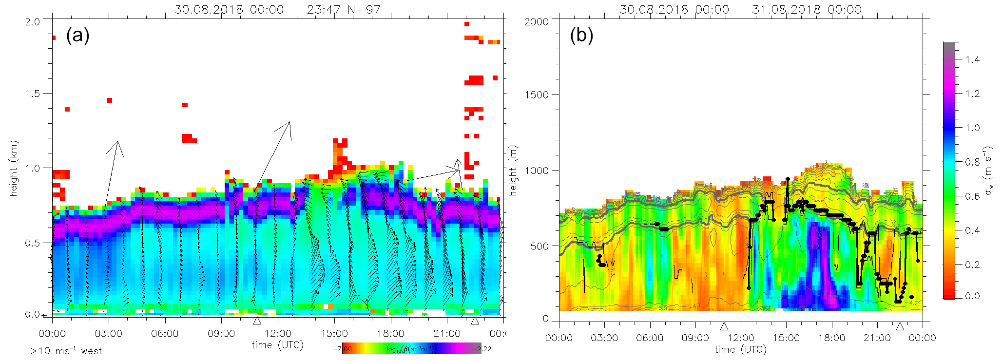
Figure A1Example data from 30 August 2018. (a) Horizontal wind speed and direction (vectors) and attenuated backscatter (β, color shading) as a function of time and height. (b) Standard deviation of vertical velocity from the wind lidar (color shading) and backscatter (log 10β, thin gray lines), with as a typical value for cloud-base (thick gray line) and mixing-layer height estimates (after Schween et al., 2014, thick black line with symbols). Note that the upper border of the region with backscatter is due to extinction of the laser signal and does not represent the cloud top. Triangles at the abscissa indicate the times of sunrise and sunset with night to the left and day on the right-hand side.

Figure A2Example data from 30 August 2018. (a) LWP and IWV from the microwave radiometer on the basis of the TH85 retrieval. (b) Potential temperature profiles from the microwave radiometer (color shading, and thin smooth lines at times indicated by dotted vertical lines) and the Antofagasta radiosonde profile for that day (thick line with symbols around 12:00 UTC). The thick gray line indicates the height of the strongest gradient. Vertical lines indicate the times of sunrise and sunset.
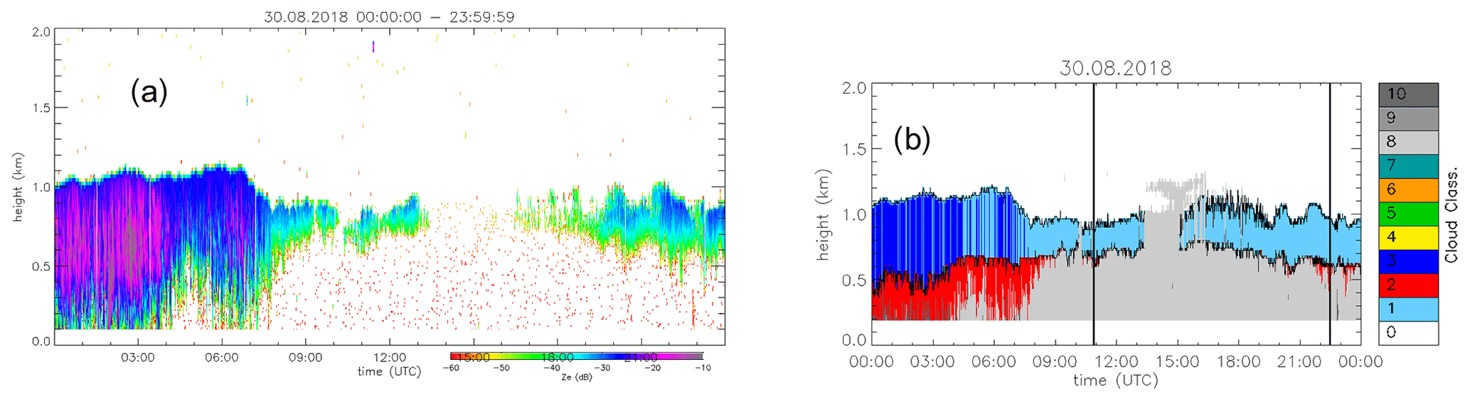
Figure A3Example data from 30 August 2018. (a) Radar reflectivity Ze from cloud radar. (b) Cloudnet classification with classes clear sky (0, white), cloud droplets only (1, light blue), drizzle or rain (2, red), drizzle or rain and cloud droplets (3, dark blue) and aerosol (8, light gray). Thin black line indicates cloud base and cloud top. Vertical lines indicate the times of sunrise and sunset.
Figures B1–B3 show example data for 19 December 2018, a typical summer day with one cloud present in the early morning, stable stratification during night, and convective turbulence reaching up to less than half of the MBL height.
Wind profiles show again during daytime stronger southwesterly winds in the lower part of the MBL and easterly winds in the upper part (Fig. B1). Nighttime winds in the lower half of the MBL are weak, with southerly to easterly directions, while above stronger westerly and northerly winds prevail. The mixed layer with vertical velocity standard deviation larger than 0.4 m s−1 reaches less than half of the MBL height. High backscatter above 900 m between 09:00 and 15:00 UTC indicates a cloud which is the source of slightly increased turbulence below, reaching down to 700 m.
MWR data reveal a low LWP around 40 g m−2 for this cloud (Fig. B2). Temperature profiles show, during the night and morning, stable stratification, which can also be found in the radio sounding from Antofagasta for this day. This stable stratification disappears around 13:00 UTC, and even super-adiabatic stratification close to the surface becomes visible. The height of the MWR inversion remains over the whole day at the same height, indicating that it is neither influenced by ground-based convection nor subsidence or divergence due to the land–sea-breeze circulation. Cloud radar reflectivity (Fig. B3) shows the cloud, and Cloudnet retrieval identifies it as a pure liquid water cloud. Its top coincides with the top of the aerosol layer (1300 m), which accordingly lies above the MWR inversion (1100 m). Cloudnet identifies in the 2 h after sunrise before 12:00 UTC drizzle for a few pixels, which is also the time with the strongest turbulence below the cloud. Nevertheless, enhanced turbulence below the cloud is also present in the following hour, indicating cooling by evaporation at the cloud top generating subsiding plumes.
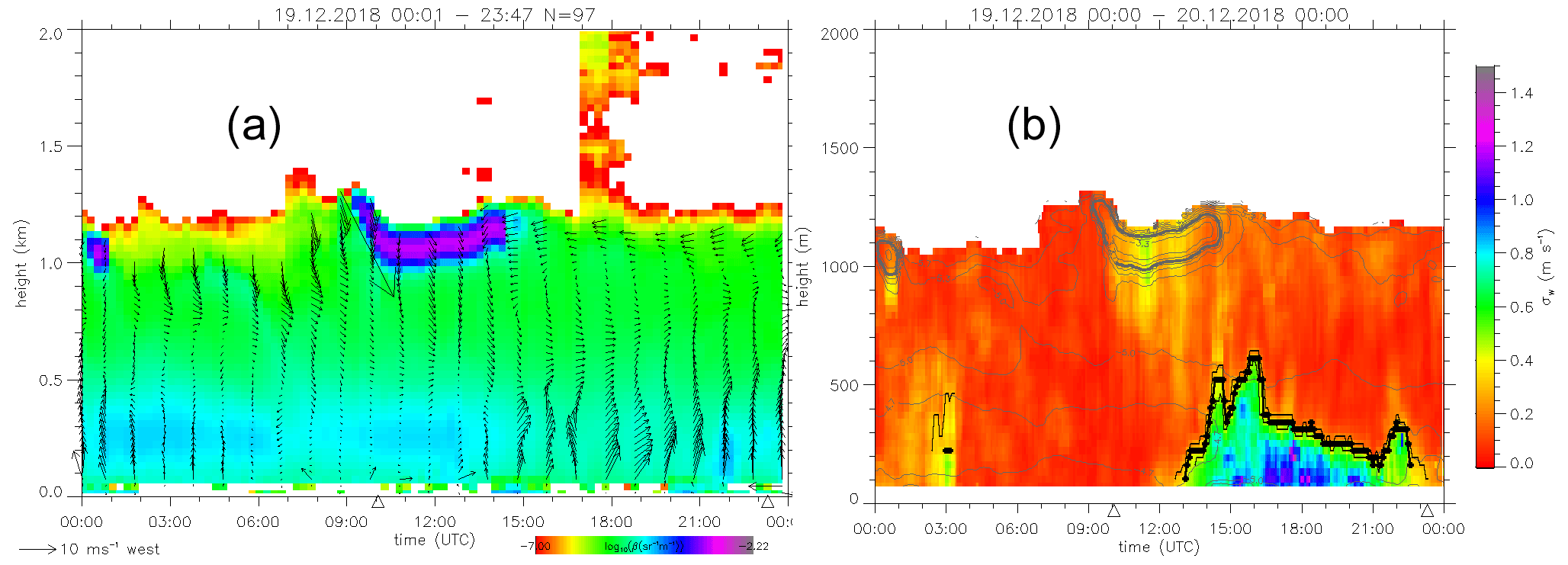

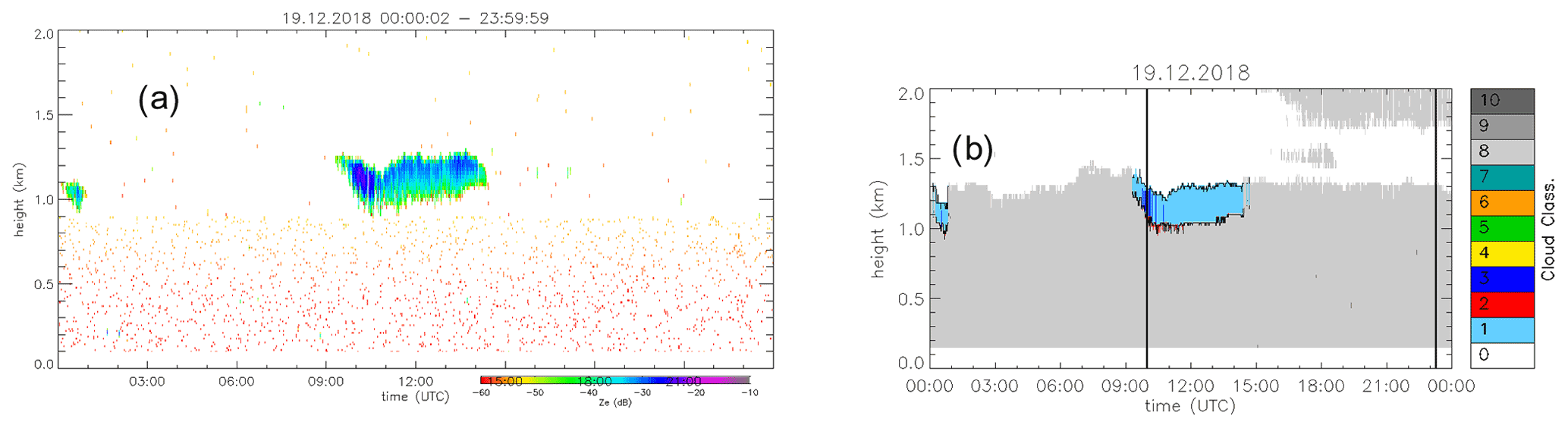
Data from wind lidar, microwave radiometer, cloud radar, and meteorological stations as well as the synergistic boundary-layer classification are accessible via the SFB 1211 Earth – Evolution at the Dry Limit project database web page (https://www.crc1211db.uni-koeln.de, last access: 6 September 2022). Basic meteorological data are available under DOI https://doi.org/10.5880/CRC1211DB.45 (Schween and Loehnert, 2022a). Wind profiles are available under DOI https://doi.org/10.5880/CRC1211DB.53 (Schween and Loehnert, 2022b). Temperature profiles are available under DOI https://doi.org/10.5880/CRC1211DB.46 (Schween et al., 2022a). LWPs for the different relative humidity thresholds are available under DOIs https://doi.org/10.5880/CRC1211DB.49 (TH80) (Schween et al., 2022b), https://doi.org/10.5880/CRC1211DB.50 (TH85) (Schween et al., 2022c), https://doi.org/10.5880/CRC1211DB.51 (TH90) (Schween et al., 2022d), and https://doi.org/10.5880/CRC1211DB.52 (TH95) (Schween et al., 2022e). IWV is available under DOI https://doi.org/10.5880/CRC1211DB.43 (Schween et al., 2022f). The boundary-layer turbulence classification is available under DOI https://doi.org/10.5880/CRC1211DB.54 (Schween et al., 2022g).
The synergistic Cloudnet classification data used in this article were generated by the European Research Infrastructure for the observation of Aerosol, Clouds and Trace Gases (ACTRIS) and are available from the ACTRIS Data Centre using the following link: https://hdl.handle.net/21.12132/2.e224164deb7c40c5 (CLU, 2022).
UL, CdR, JLG, and PO planned the campaign and selected the site. SW and JHS did the data analysis. UL, SW, and JHS planned and structured the paper. JHS wrote the manuscript. JHS, CdR, JLG, PO, SW, and UL reviewed it iteratively.
The contact author has declared that none of the authors has any competing interests.
Publisher’s note: Copernicus Publications remains neutral with regard to jurisdictional claims in published maps and institutional affiliations.
Data analysis procedures and retrievals are developed at the University of Cologne through the joint efforts at CPEX-LAB (http://www.cpex-lab.de, last access: 2 February 2022). We are grateful to Anne Hirsikko and Heikki Lihavainen from the Finnish Meteorological Institute (FMI) for providing the Doppler lidar for this installation. We are grateful to the Dirección General De Aeronáutica Civil, Departamento Comercial (DGAC) for giving their permission to install the instruments on the grounds of Diego Aracena Airport at Iquique and Marcial Vidal Arriagada for support from the side of the airport management. We thank Clara Stock from the Centre for Organismal Studies, University of Heidelberg, and Constanza Vargas from the Centro UC Desierto de Atacama for maintenance and technical support of the instruments during their installation at Iquique Airport. We thank the ACTRIS Cloud Profiling Unit (CLU) for providing the dataset in this study, which was produced by the Finnish Meteorological Institute. We especially thank Ewan O'Connor from the FMI for including the instruments in the Cloudnet operational processing and Tobias Marke for setting up the turbulence classification scheme. Both of these contributions are based on collaborative efforts within the EU COST Action PROBE (CA1835) “Profiling the atmospheric boundary layer at European scale”. This work would not have been possible without our technicians Pavel Krobot and Rainer Haseneder-Lind and their efforts in preparing, packing, and sending the instruments, setting up and maintaining the Internet connection, and support on the way back. We also thank Susanne Crewell and Thomas Rose for assisting during the instrument setup. Finally, the authors are very grateful for the efforts of Mario Mech, whose experienced support in preparing and carrying out the setup of the measurement station was indispensable to the success of the project.
The project has been funded by the Deutsche Forschungsgemeinschaft (DFG, German Research Foundation) Collaborative Research Centre 1211 Earth – Evolution at the Dry Limit (SFB 1211, project no. 268236062).
This paper was edited by Matthew Lebsock and reviewed by two anonymous referees.
Böhm, C., Schween, J., Reyers, M., Maier, B., Löhnert, U., and Crewell, S.: Towards a climatology of fog frequency in the Atacama Desert via multi-spectral satellite data and machine learning techniques, J. Appl. Meteorol. Clim., 60, 1149–1169, https://doi.org/10.1175/JAMC-D-20-0208.1, 2021. a
Bretherton, C. S., Uttal, T., Fairall, C. W., Yuter, S. E., Weller, R. A., Baumgardner, D., Comstock, K., Wood, R., and Raga, G.: The Epic 2001 Stratocumulus Study., B. Am. Meteorol. Soc., 85, 967–978, https://doi.org/10.1175/BAMS-85-7-967, 2004. a, b, c, d
Cereceda, P., Larrain, H., Osses, P., Farías, M., and Egaña, I.: The spatial and temporal variability of fog and its relation to fog oases in the Atacama Desert, Chile, Atmos. Res., 87, 312–323, https://doi.org/10.1016/j.atmosres.2007.11.012, 2008a. a
Cereceda, P., Larrain, H., Osses, P., Farías, M., and Egaña, I.: The climate of the coast and fog zone in the Tarapacá Region, Atacama Desert, Chile, Atmos. Res., 32, 1803–1814, https://doi.org/10.1016/j.atmosres.2007.11.011, 2008b. a
CLU: Cloud profiling product: Classification; 2018-03-26 to 2019-01-23; from Iquique, ACTRIS Data Centre [data set], https://hdl.handle.net/21.12132/2.e224164deb7c40c5, last access: 2 February 2022. a
Crewell, S. and Löhnert, U.: Accuracy of boundary layer temperature profiles retrieved with multi-frequency, multi-angle microwave radiometry, IEEE T. Geosci. Remote, 45, 2195–2201, https://doi.org/10.1109/TGRS.2006.888434, 2007. a, b
del Rio, C., Lobos-Roco, F., Koch, M., García, J.-L., Osses, P., Lambert, F., Alfaro, F., and Siegmund, A.: Spatial distribution and interannual variability of coastal fog and low clouds cover in the hyperarid Atacama Desert and implications for past and present Tillandsia landbeckii ecosystems, Plant Syst. Evol., 307, 58, https://doi.org/10.1007/s00606-021-01782-z, 2021a. a, b, c, d
del Rio, C., Lobos-Roco, F., Siegmund, A., Tejos, C., Osses, P., Huaman, Z., Meneses, J., and García, J.-L.: GOFOS, ground optical fog observation system for monitoring the vertical stratocumulus-fog cloud distribution in the coast of the Atacama Desert, Chile, J. Hydrol., 597, 126190, https://doi.org/10.1016/j.jhydrol.2021.126190, 2021b. a, b, c
Direccion Meteorologica de Chile (DMC) Servicios Climaticos: Metadata and data from Meteorological station 200006 (Diego Aracena Iquique Ap.), DMC [data set], https://climatologia.meteochile.gob.cl/application/informacion/fichaDeEstacion/200006, last access: 26 April 2022, 2022. a, b
Dunai, T., Melles, M., Quandt, D., Knief, C., and Amelung, W.: Whitepaper: Earth – Evolution at the dry limit, Global Planet. Change, 193, 103275, https://doi.org/10.1016/j.gloplacha.2020.103275, 2020. a
García, J.-L., Lobos-Roco, F., Schween, J., del Rio, C., Vives, R., Pezoa, M., Siegmund, A., Latorre, C., Alfaro, F., Koch, M., and Löhnert, U.: Climate and coastal low-cloud dynamic in the hyperarid Atacama fog Desert and the geographic distribution of Tillandsia landbeckii (Bromeliaceae) dune ecosystems, Plant Syst. Evol., 307, 57, https://doi.org/10.1007/s00606-021-01775-y, 2021. a, b
Illingworth, A. J., Hogan, R. J., O'Connor, E., Bouniol, D., Brooks, M. E., Delanoé, J., Donovan, D. P., Eastment, J. D., Gaussiat, N., Goddard, J. W. F., Haeffelin, M., Klein Baltink, H., Krasnov, O. A., Pelon, J., Piriou, J.-M., Protat, A., Russchenberg, H. W. J., Seifert, A., Tompkins, A. M., van Zadelhoff, G.-J., Vinit, F., Willén, U., Wilson, D. R., and Wrench, C. L.: CLOUDNET Continous evaluation of cloud profiles in seven operational models using ground-based observations, B. Am. Meteorol. Soc., 88, 883–898, https://doi.org/10.1175/BAMS-88-6-883, 2007. a
Karstens, U., Simmer, C., and Ruprecht, E.: Remote sensing of cloud liquid water, Meteorol. Atmos. Phys., 54, 157–171, https://doi.org/10.1007/BF01030057, 1994. a
Klein, S. and Hartmann, D.: The seasonal cycle of low stratiform clouds, J. Climate, 6, 1587–1606, https://doi.org/10.1175/1520-0442(1993)006<1587:TSCOLS>2.0.CO;2, 1993. a
Küchler, N., Kneifel, S., Löhnert, U., Kollias, P., Czekala, H., and Rose, T.: A W-Band Radar–Radiometer System for Accurate and Continuous Monitoring of Clouds and Precipitation, J. Atmos. Ocean. Tech., 34, 2375–2392, https://doi.org/10.1175/JTECH-D-17-0019.1, 2017. a
Lawrence, M.: The relationship between relative humidity and the dewpoint temperature in moist air: A simple conversion and applications, B. Am. Meteorol. Soc., 86, 225–233, https://doi.org/10.1175/BAMS-86-2-225, 2005. a
Lilly, D. K.: Models of cloud-topped mixed layers under a strong inversion, Q. J. Roy. Meteor. Soc., 94, 292–309, https://doi.org/10.1002/qj.49709440106, 1968. a
Lin, J., Qian, T., and Shinoda, T.: Stratocumulus Clouds in Southeastern Pacific Simulated by Eight CMIP5–CFMIP Global Climate Models, J. Climate, 27, 3000–3022, https://doi.org/10.1175/JCLI-D-13-00376.1, 2012. a, b
Lobos-Roco, F., Vilá-Guerau de Arellano, J., and Pedruzo-Bagazgoitia, X.: Characterizing the influence of the marine stratocumulus cloud on the land fog at the Atacama Desert, Atmos. Res., 214, 109–120, https://doi.org/10.1016/j.atmosres.2018.07.009, 2018. a
Löhnert, U. and Crewell, S.: Accuracy of cloud liquid water path from groundbased microwave radiometry 1. Dependency on cloud model statistics, Radio Sci., 38, 8041, https://doi.org/10.1029/2002RS002654, 2003. a
Löhnert, U., Turner, D., and Crewell, S.: Ground-based temperature and humidity profiling using spectral infrared and microwave observations: Part 1. Simulated retrieval performance in clear sky conditions, J. Appl. Meteorol. Clim., 48, 1017–1032, https://doi.org/10.1175/2008JAMC2060.1, 2009. a
Manninen, A., Marke, T., O'Connor, E., and Tuononen, M.: Atmospheric boundary layer classification with Doppler lidar, J. Geophys. Res., 123, 8172–8189, https://doi.org/10.1029/2017JD028169, 2018. a, b
Manrique, R.: El Niño Southern Oscillation And Its Effect On Fog Oases Along The Peruvian And Chilean Coastal Deserts, PhD thesis, Universita di Bologna, http://amsdottorato.unibo.it/3436/1/Manrique_Rosa_tesi.pdf (last access: 22 February 2022), 2011. a
Martucci, G., Milroy, C., and O'Dowd, C. D.: Detection of Cloud-Base Height Using Jenoptik CHM15K and Vaisala CL31 Ceilometers, J. Atmos. Ocean. Tech., 27, 305–318, https://doi.org/10.1175/2009JTECHA1326.1, 2010. a, b
Mechoso, C. R., Wood, R., Weller, R., Bretherton, C., Clarke, A. D., Coe, H., Fairall, C., Farrar, J. T., Feingold, G., Garreaud, R., Grados, C., McWilliams, J., de Szoeke, S. P., Yuter, S. E., and Zuidema, P.: Ocean–Cloud–Atmosphere–Land Interactions In The Southeastern Pacific, The Vocals Program, B. Am. Meteorol. Soc., 95, 357–375, https://doi.org/10.1175/BAMS-D-11-00246.1, 2014. a, b
Muñoz, R., Zamora, R. A., and Rutllant, J. A.: The Coastal Boundary Layer at the Eastern Margin of the Southeast Pacific (23.48∘ S, 70.48∘ W): Cloudiness-Conditioned Climatology, J. Climate, 24, 1013–1033, https://doi.org/10.1175/2010JCLI3714.1, 2011. a
Muñoz, R., Quintana, J., Falvey, M. J., Rutllant, J. A., and Garreaud, R. D.: Coastal Clouds at the Eastern Margin of the Southeast Pacific: Climatology and Trends, J. Climate, 29, 4525–4542, https://doi.org/10.1175/JCLI-D-15-0757.1, 2016. a, b, c, d, e, f
Muñoz, R. C. and Garreaud, R. D.: Dynamics of the Low-Level Jet off the West Coast of Subtropical South America, Mon. Weather Rev., 133, 3661–3677, https://doi.org/10.1175/MWR3074.1, 2005. a
Muñoz-Schick, M., Pinto, R., Mesa, A., and Moreira-Muñoz, A.: Fog oases during the El Niño Southern Oscillation 1997–1998, in the coastal hills south of Iquique, Tarapacá region, Chile, Revist Chilena de Historia Natural, 74, 389–405, https://doi.org/10.4067/S0716-078X2001000200014, 2001. a
Naval Oceanographic Office: K10 Global 10 km Analyzed SST data set. Ver. 1.0., Physical Oceanography Distributed Active Archive center (PO.DAAC) CA, USA [data set], https://doi.org/10.5067/GHK10-41N01, 2008. a, b, c, d
Naval Oceanographic Office: GHRSST L4 NAVO K10 Global 1m-depth Analyzed SST dataset. Ver. 1.0., Physical Oceanography Distributed Active Archive center (PO.DAAC) CA, USA [data set], https://doi.org/10.5067/GHK10-L4N01, 2018. a, b, c
NOAA Climate Prediction Center: ENSO ONI index, https://origin.cpc.ncep.noaa.gov/products/analysis_monitoring/ensostuff/ONI_v5.php, last access: 2 February 2022. a
Ouwersloot, H. and Vila-Guerau de Arellano, J.: Analytical Solution for the Convectively-Mixed Atmospheric Boundary Layer, Bound.-Lay. Meteorol., 148, 557–583, https://doi.org/10.1007/s10546-013-9816-z, 2013. a
Päschke, E., Leinweber, R., and Lehmann, V.: An assessment of the performance of a 1.5 µm Doppler lidar for operational vertical wind profiling based on a 1-year trial, Atmos. Meas. Tech., 8, 2251–2266, https://doi.org/10.5194/amt-8-2251-2015, 2015. a
Romps, D.: Exact Expression for the Lifting Condensation Level, J. Atmos. Sci., 74, 3891–3900, https://doi.org/10.1175/JAS-D-17-0102.1, 2017. a
Rose, T., Crewell, S., Löhnert, U., and Simmer, C.: A network suitable microwave radiometer for operational monitoring of the cloudy atmosphere, Atmos. Res., 75, 183–200, https://doi.org/10.1016/j.atmosres.2004.12.005, 2005. a
Rutllant, J., Fuenzalida, H., and Aceituno, P.: Climate dynamics along the arid northern coast of Chile: The 1997–1998 Dinámica del Clima de la Región de Antofagasta (DICLIMA) experiment, J. Geophys. Res., 108, 4538, https://doi.org/10.1029/2002JD003357, 2003. a
Schneider, T., Kaul, C., and Pressel, K.: Possible climate transitions from breakup of stratocumulus decks under greenhouse warming, Nat. Geosci., 12, 163–167, https://doi.org/10.1038/s41561-019-0310-1, 2019. a
Schubert, W., Wakefield, J., Steiner, E., and Cox, S.: Marine Stratocumulus Convection. Part I: Governing Equations and Horizontally Homogeneous Solutions, J. Atmos. Sci., 36, 1286–1307, https://doi.org/10.1175/1520-0469(1979)036<1286:MSCPIG>2.0.CO;2, 1979. a, b
Schulz, N., Boisier, J. P., and Aceituno, P.: Climate change along the coast of northern Chile, Int. J. Climatatol., 36, 1308–1324, https://doi.org/10.1175/1520-0469(1979)036<1308:MSCPIH>2.0.CO;2, 2012. a, b, c
Schween, J., Hoffmeister, D., and Löhnert, U.: Filling the Observational Gap in the Atacama Desert with a new Network of Climate Stations, Global Planet. Change, 184, 103034, https://doi.org/10.1016/j.gloplacha.2019.103034, 2020. a, b, c
Schween, J. H. and Loehnert, U.: Meteorological Data March 2018–March 2019 from Iquique, CRC1211 Database (CRC1211DB) [data set], https://doi.org/10.5880/CRC1211DB.45, 2022a. a
Schween, J. H. and Loehnert, U.: Wind profiles March 2018–March 2019 from remote sensing at Iquique, CRC1211 Database (CRC1211DB) [data set], https://doi.org/10.5880/CRC1211DB.53, 2022b. a
Schween, J. H., Hirsikko, A., Löhnert, U., and Crewell, S.: Mixing-layer height retrieval with ceilometer and Doppler lidar: from case studies to long-term assessment, Atmos. Meas. Tech., 7, 3685–3704, https://doi.org/10.5194/amt-7-3685-2014, 2014. a, b
Schween, J. H., Loehnert, U., and Westbrook, S.: Temperature profiles March 2018–March 2019 from remote sensing at Iquique, CRC1211 Database (CRC1211DB) [data set], https://doi.org/10.5880/CRC1211DB.46, 2022a. a
Schween, J. H., Loehnert, U., and Westbrook, S.: Liquid water path (LWP TH80) March 2018–March 2019 at Iquique, CRC1211 Database (CRC1211DB) [data set], https://doi.org/10.5880/CRC1211DB.49, 2022b. a
Schween, J. H., Loehnert, U., and Westbrook, S.: Liquid water path (LWP TH85) March 2018–March 2019 at Iquique, CRC1211 Database (CRC1211DB) [data set], https://doi.org/10.5880/CRC1211DB.50, 2022c. a
Schween, J. H., Loehnert, U., and Westbrook, S.: Liquid water path (LWP TH90) March 2018–March 2019 at Iquique, CRC1211 Database (CRC1211DB) [data set], https://doi.org/10.5880/CRC1211DB.51, 2022d. a
Schween, J. H., Loehnert, U., and Westbrook, S.: Liquid water path (LWP TH95) March 2018–March 2019 at Iquique, CRC1211 Database (CRC1211DB) [data set], https://doi.org/10.5880/CRC1211DB.52, 2022e. a
Schween, J. H., Loehnert, U., and Westbrook, S.: Integrated water vapor (IWV TH85) March 2018–March 2019 at Iquique, CRC1211 Database (CRC1211DB) [data set], https://doi.org/10.5880/CRC1211DB.43, 2022f. a
Schween, J. H., Marke, T., and Loehnert, U.: Boundary layer classification from remote sensing at Iquique, March 2018–March 2019, CRC1211 Database (CRC1211DB) [data set], https://doi.org/10.5880/CRC1211DB.54, 2022g. a
Serpetzoglou, E., Albrecht, B., Kollias, P., and Fairall, C.: Boundary Layer, Cloud, and Drizzle Variability in the Southeast Pacific Stratocumulus Regime, J. Climate, 21, 6191–6214, https://doi.org/10.1175/2008JCLI2186.1, 2008. a
Stevens, B., Lenschow, D. H., Vali, G., Gerber, H., Bandy, A., Blomquist, B., Brenguier, J.-L., Bretherton, C. S., Burnet, F., Campos, T., Chai, S., Faloona, I., Friesen, D., Haimov, S., Laursen, K., Lilly, D. K., Loehrer, S. M., Malinowski, S. P., Morley, B., Petters, M. D., Rogers, D. C., Russell, L., Savic-Jovcic, V., Snider, J. R., Straub, D., Marcin, D., Szumowski, J., Takagi, H., Thornton, D. C., Tschudi, M., Twohy, C., Wetzel, M., and Van Zanten, M. C.: Dynamics and Chemistry of Marine Stratocumulus – DYCOMS-II, B. Am. Meteorol. Soc., 84, 579–593, https://journals.ametsoc.org/view/journals/bams/84/5/bams-84-5-579.xml (last access: 5 September 2022), 2003. a, b
Stevens, B., Moeng, C., Ackerman, A. S., Bretherton, C. S., Chlond, A., de Roode, S., Edwards, J., Golaz, J., Jiang, H., Khairoutdinov, M., Kirkpatrick, M. P., Lewellen, M. P., Lock, A., Müller, F., Stevens, M. P., Whelan, E., and Zhu, P.: Evaluation of Large-Eddy Simulations via Observations of Nocturnal Marine Stratocumulus, Mon. Weather Rev., 133, 1443–1462, https://doi.org/10.1175/MWR2930.1, 2005. a
Tuononen, M., O'Connor, E. J., and Sinclair, V. A.: Evaluating solar radiation forecast uncertainty, Atmos. Chem. Phys., 19, 1985–2000, https://doi.org/10.5194/acp-19-1985-2019, 2019. a, b
Turton, J. D. and Nicholls, S.: A study of the diurnal variation of stratocumulus using a multiple mixed layer model, Q. J. Roy. Meteor. Soc., 113, 969–1009, https://doi.org/10.1002/qj.49711347712, 1987. a
Wood, R.: Stratocumulus clouds, Mon. Weather Rev., 140, 2373–2423, https://doi.org/10.1175/MWR-D-11-00121.1, 2012. a, b, c, d, e, f, g
Wood, R., Mechoso, C. R., Bretherton, C. S., Weller, R. A., Huebert, B., Straneo, F., Albrecht, B. A., Coe, H., Allen, G., Vaughan, G., Daum, P., Fairall, C., Chand, D., Gallardo Klenner, L., Garreaud, R., Grados, C., Covert, D. S., Bates, T. S., Krejci, R., Russell, L. M., de Szoeke, S., Brewer, A., Yuter, S. E., Springston, S. R., Chaigneau, A., Toniazzo, T., Minnis, P., Palikonda, R., Abel, S. J., Brown, W. O. J., Williams, S., Fochesatto, J., Brioude, J., and Bower, K. N.: The VAMOS Ocean-Cloud-Atmosphere-Land Study Regional Experiment (VOCALS-REx): goals, platforms, and field operations, Atmos. Chem. Phys., 11, 627–654, https://doi.org/10.5194/acp-11-627-2011, 2011. a
Zhou, X., Kollias, P., and Lewis, E. R.: Clouds, Precipitation, and Marine Boundary Layer Structure during the MAGIC Field Campaign, J. Climate, 28, 2420–2442, https://doi.org/10.1175/JCLI-D-14-00320.1, 2015. a