Summer variability of the atmospheric NO₂ :  NO ratio at Dome C on the East Antarctic Plateau

Previous Antarctic summer campaigns have shown unexpectedly high levels of oxidants in the lower atmosphere of the continental plateau and at coastal regions, with atmospheric hydroxyl radical (OH) concentrations up to 4 × 10⁶ cm⁻³. Such high reactivity in the summer Antarctic boundary layer results in part from the emissions of nitrogen oxides (NO_x ≡ NO + NO₂) produced during photo-denitrification of the snowpack, but its underlying mechanisms are not yet fully understood, as some of the chemical species involved (NO₂, in particular) have not yet been measured directly and accurately. To overcome this crucial lack of information, newly developed optical instruments based on absorption spectroscopy (incoherent broadband cavity-enhanced absorption spectroscopy, IBBCEAS) were deployed for the first time at Dome C (−75.10 lat., 123.33 long., 3233 m a.s.l.) during the 2019–2020 summer campaign to investigate snow–air–radiation interaction. These instruments directly measure NO₂ with a detection limit of 30 pptv (parts per trillion by volume or 10⁻¹² mol mol⁻¹) (3σ). We performed two sets of measurements in December 2019 (4 to 9) and January 2020 (16 to 25) to capture the early and late photolytic season, respectively. Late in the season, the daily averaged NO₂:NO​​​​​​​ ratio of 0.4 ± 0.4 matches that expected for photochemical equilibrium through Leighton's extended relationship involving RO_x (0.6 ± 0.3). In December, however, we observed a daily averaged NO₂:NO ratio of 1.3 ± 1.1, which is approximately twice the daily ratio of 0.7 ± 0.4 calculated for the Leighton equilibrium. This suggests that more NO₂ is produced from the snowpack early in the photolytic season (4 to 9 December), possibly due to stronger UV irradiance caused by a smaller solar zenith angle near the solstice. Such a high sensitivity of the NO₂:NO ratio to the sun's position is of importance for consideration in atmospheric chemistry models.

1 Introduction

Intense field campaigns over the past 3 decades have studied the Arctic and Antarctic boundary layer composition and photochemistry (Bauguitte et al., 2012, and references therein). The relatively unpolluted nature of these regions, free of local anthropogenic emissions, has led to the growing interest in their atmospheric chemistry and the collection and interpretation of polar ice cores (Wolff, 1995). Antarctica, in particular, is the most isolated continent on Earth; therefore, providing the most suitable continent-scale laboratory for studying past and present natural atmospheric cycles (EPICA community members, 2004). Because of this presumed pristine nature, the scientific community was puzzled by initial observations of high oxidative capacity in the polar boundary layer, i.e. an oxidation process initiated by oxidants (including ozone, hydroxyl and peroxyl radicals, hydrogen peroxide, halogen radicals), which resembled those seen in urban environments (Beine et al., 2002; Mauldin et al., 2001; Davis et al., 2001; Jones et al., 2008; Kukui et al., 2014; Preunkert et al., 2012; Saiz-Lopez et al., 2008). It is today well established that such high reactivity in the summer Antarctic boundary layer results from the presence of highly reactive species, such as nitrogen oxides (NO_y ≡ NO, NO₂, HONO, HO₂NO₂, HNO₃ etc.), hydroxyl and peroxyl radicals (RO_x ≡ OH, HO₂, RO₂), and halogen oxides (XO ≡ BrO, IO, ClO), due to precursor emissions from the snowpack (Davis et al., 2008; Anderson and Bauguitte, 2007; Preunkert et al., 2012, and references therein). Despite their short lifetime and low abundance in the atmosphere, they control the oxidative capacity and the atmospheric chemistry of these regions due to their high reactivity. Today, this phenomenon is still not yet fully understood due to the difficulty of performing accurate and free of interference NO_x measurements, combined with a complex oxidation–reduction reaction involving NO_x, O₃, and radicals in the snow and atmosphere at wavelengths, λ, below 420 nm (Fig. 1).

1. The photolysis of nitrate ions (NO${}_{\mathrm{3}}^{-}$) in the snow produces NO_x (≡ NO₂ + NO) (Grannas et al., 2007). Gas-phase nitrogen dioxide (NO₂) photolyses to produce nitrogen oxide (NO), which also results in production of ozone (O₃), which then reacts together to reform NO₂ (bold cycle in Fig. 1-1). In this recycling reaction, no net production or loss of any species is involved.

2. However, in the presence of other species, such as peroxyl radicals (RO_x) or halogenated radicals (XO), NO can produce NO₂ without consuming O₃ (Fig. 1-2).

3. NO₂ can also be consumed by reacting with hydroxyl or halogenated radicals to form HNO₃, which will redeposit onto the snowpack surface (Fig. 1-3).

4. Additionally, NO can react with OH to form HONO (Fig. 1-4), which was measured on the Antarctic Plateau during the OPALE campaign. HONO has been modelled to be present at around 8 to 12 pptv (parts per trillion by volume or 10⁻¹² mol mol⁻¹) during the austral summer (Legrand et al., 2014). However, Legrand et al. (2014) showed that the oxidation of NO by the OH radical is not sufficient to explain the levels of HONO observed.

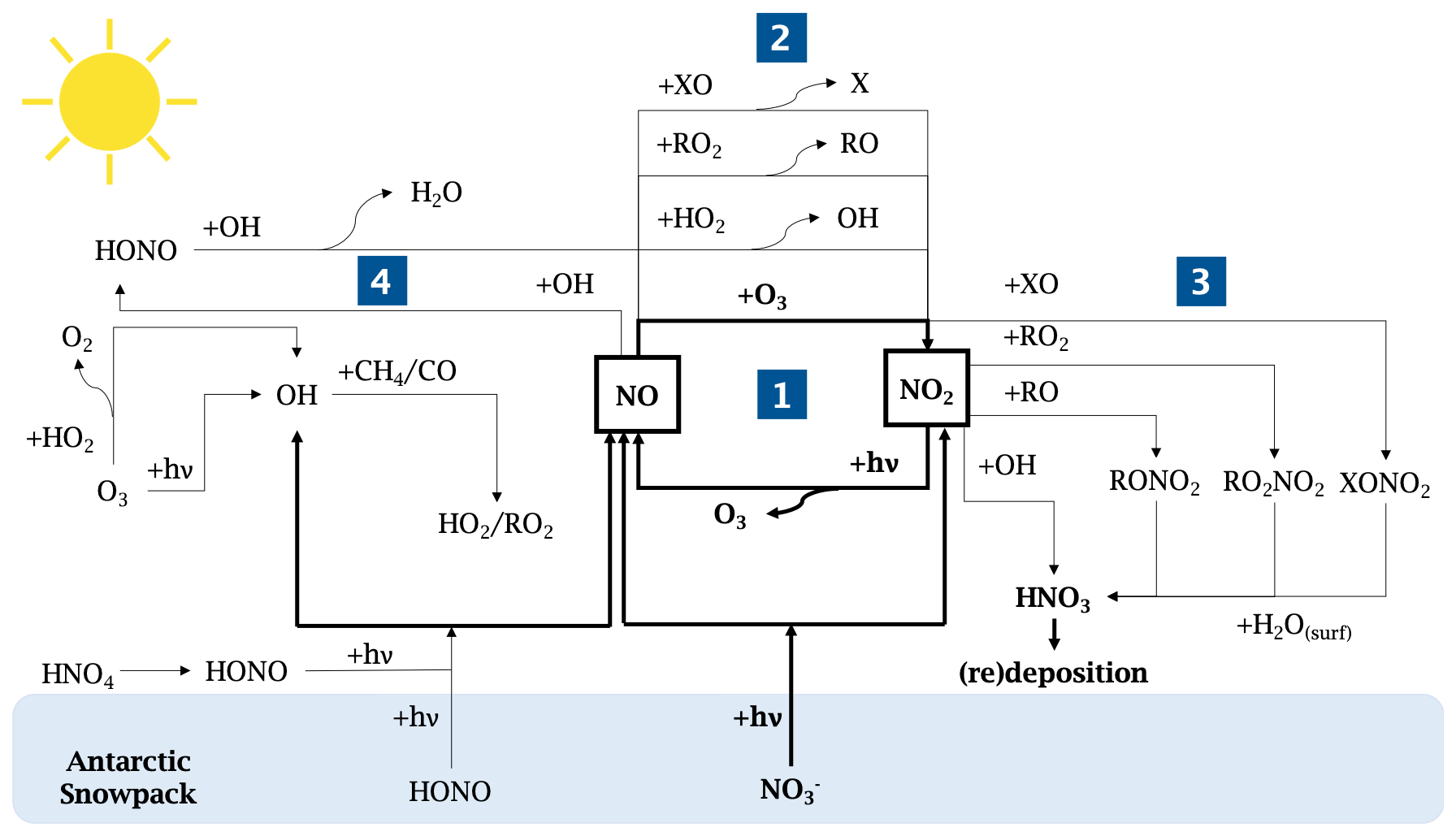
Figure 1 Schematic of the NO_x chemistry in the Antarctic Plateau. The NO_x cycle and the NO_x direct snow sources are shown in bold.​​​​​​​

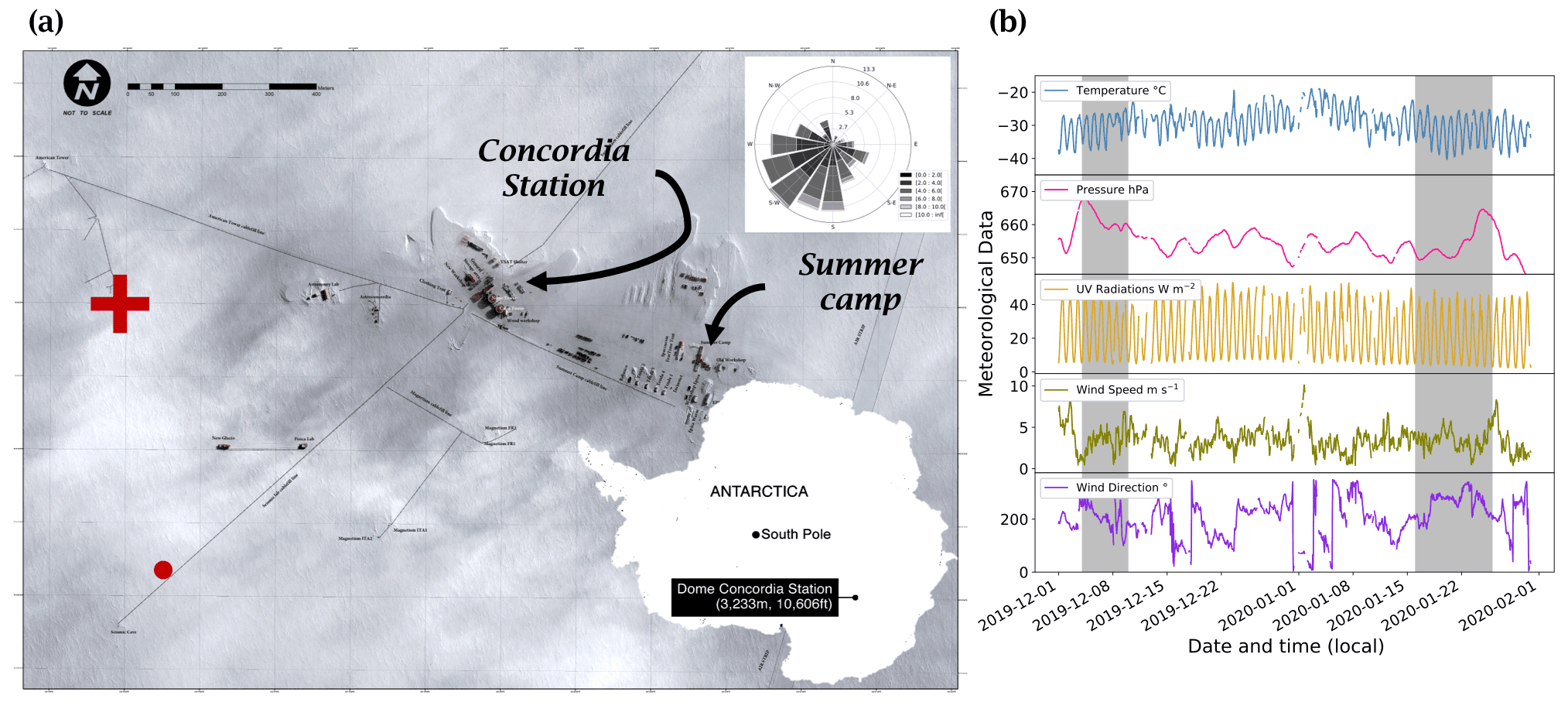
Figure 2 (a) Satellite view of the station. The red cross marks the position of the atmospheric observations, and the red dot marks the location of the automatic weather station (AWS, Vaisala Milos 520). The wind rose for the period 1 December 2019 to 31 January 2020 is shown in the upper right-hand corner (Pléiade satellite image of Concordia Station, Antarctica, © CNES 2016, Distribution Airbus Defence and Space). (b) Local meteorological conditions (2 m observations) measured for the period 1 December 2019 to 31 January 2020 by the local automatic weather station (Vaisala Milos 520) completed with a broadband UV radiometer (spectral range 305–385 nm). The shaded areas represent the periods when atmospheric chemistry measurements were conducted.

The following list of campaigns and publications is not exhaustive but gives an idea of the intensive studies of the Antarctic atmospheric chemistry for evaluating the air–snow transfer function. ISCAT 2000 (Investigation of Sulfur Chemistry of the Antarctic Troposphere) at South Pole station in 2000 (Berresheim and Eisele, 1998; Davis et al., 2004) revealed a strong oxidizing environment at South Pole (SP). The measurements established the recycling of reactive nitrogen as a critical component of this unique environment. ANTCI (The Antarctic Tropospheric Chemistry Investigation) deployed two field studies between 2003 and 2005 with large ground-based sampling during winter components at SP station and aircraft chemistry and photochemistry measurements (Davis et al., 2008; Eisele et al., 2008; Helmig et al., 2008; Wang et al., 2007). The CHABLIS (CHemistry of the Antarctic Boundary Layer and the Interface with Snow) measurement campaign was conducted at Halley station in coastal Antarctica from January 2004 through February 2005 (Anderson and Bauguitte, 2007; Bauguitte et al., 2012; Bloss et al., 2007, 2010; Jones et al., 2008, 2011; Mills et al., 2007; Read et al., 2008; Saiz-Lopez et al., 2008; Salmon et al., 2008; Wolff et al., 2008). SUNITE DC (Sulfate and NItraTe surface snow Evolution at Dome C) aimed to document and use isotopic anomalies of oxyanions (sulfate and nitrate) to constrain the sources, transformations, and transports of these compounds to the polar regions where they are archived over thousands of years (Bock et al., 2016; Erbland et al., 2013; Meusinger et al., 2014; Savarino et al., 2007; Vicars and Savarino, 2014; Frey et al., 2009). The OPALE (Oxidative Production over Antarctic Land and its Export) campaign took place at both coastal Antarctica (Terre Adélie, Dumont D'Urville station) and the plateau (Dome C, Concordia station), with the aim to quantify, understand, and model the level of oxidants present in the lower atmosphere of East Antarctica (Berhanu et al., 2015; Erbland et al., 2015; Frey et al., 2013, 2015; Gallée et al., 2015a, b; Kukui et al., 2014; Legrand et al., 2014, 2016; Preunkert et al., 2012, 2015; Savarino et al., 2016). Despite the numerous observations of nitrogen-bearing species, i.e. HONO, NO_x, and NO, collected during those cited previous campaigns, no direct NO₂ measurements, free of interferences from other NO_x species (Frey et al., 2013, 2015; Legrand et al., 2014), have so far been performed on the Antarctic plateau. Indeed, previous studies used chemiluminescent detectors (CLDs), which directly measure NO and estimate NO_x and NO₂ from photolytic conversion to NO, which is conversion that is subject to interferences. This absence hinders our efforts to correctly evaluate the NO_x cycle over the snowpack, leaving significant uncertainties in modelled values, which affect our full understanding of snow–air–radiation interactions. To overcome this lack of information, direct and accurate NO₂ measurements with simultaneous detection of NO are needed. Here, we deployed newly developed optical instruments that allow direct measurement of NO₂ and indirect measurement of NO with detection limits of 30 and 63 pptv (3σ), respectively (Barbero et al., 2020). Although indirect, the NO measurement is well constrained. Potential artefacts have been identified and discussed in Barbero et al. (2020). Even though they may occur during night-time in an urban polluted environment, caused by the presence of N₂O₅, they are negligible during the summer period in Antarctica. We present new results on summer NO₂:NO variability over the Antarctic Plateau and explore the mechanisms involved in the atmospheric boundary layer of the Antarctic Plateau during the photolytic season in light of these new data. While the overall NO₂:NO ratio can be explained by the extended Leighton's relationship (including peroxy radicals, RO_x), a high NO₂:NO ratio was estimated in the morning during the early photolysis season, deviating from steady-state equilibrium and not explained by the extended Leighton's relationship taken from Ridley et al. (2000). Additionally, calculations show that the previous assumption of an additional conversion of NO to NO₂ through XO or RO_x is insufficient to fully explain the observations. In this work, using results of dynamic flux chamber experiments, (Barbero et al., 2021), which allowed the NO_x snow source to be better characterized, we were able to highlight that the NO₂:NO ratio is very sensitive to the position of the sun. Indeed, results show that a 5 % difference in the solar zenith angle (SZA) between December and January may explain the equilibrium deviation observed in the NO₂:NO ratio during the summer campaign.

2 Methods

2.1 Site description, sampling location, and set-up

Atmospheric NO_x measurements were conducted for a total of 16 d, from 4 to 9 December 2019 and from 16 to 25 January 2020, at the French–Italian Concordia Station, Dome C, Antarctica (−75.10 lat., 123.33 long., 3233 m a.s.l.). This year-round-operating station is located on the Antarctic Plateau at a distance of 1100 km from the coast and provides an exceptional site for studying polar atmospheric chemistry. The station experiences polar night during the austral winter when the sun remains below the horizon from May to August, while in summer (November to January) the SZA has a minimum of 52^∘, i.e. the sun is at maximum 38^∘ above the horizon. The local weather is generally dominated by cold, clear, and calm conditions. The annual wind speed, W_speed-mean=4.0 ± 2.1 m s⁻¹, is low due to its sitting at the top of a dome at an altitude of more than 3200 m. Occasional regional storm systems can advect more coastal air masses associated with higher wind speeds and relatively warmer and cloudier weather (Genthon et al., 2010). The meteorological conditions encountered during the summer campaign (Fig. 2) were typical of summer climatology (November to February) observed at Dome C: $T_{\mathrm{mean}}=-\mathrm{29}$ ± 4 ^∘C; P_mean=655 ± 4 hPa; W_speed-mean=3.5 ± 1.5 m s⁻¹; W_dir-mean=206 ± 71^∘; and UV_mean=24 ± 15 W m⁻² (spectral range 305–385 nm). The 5 d back trajectories conducted by the HYSPLIT (Hybrid Single-Particle Lagrangian Integrated Trajectory) transport and dispersion model (Stein et al., 2015; Rolph et al., 2017, https://www.ready.noaa.gov, last access: 7 October 2021) show that the air masses were principally coming from the continent during the measurement periods (more information is provided in Appendix A). The meteorological conditions encountered during both atmospheric measurement periods can be found in Appendix B.

Atmospheric sampling was done in the station's clean area sector (a zone less subject to pollution linked to the station's activities), about 1 km south-west and upwind of the main station buildings (Fig. 2). A laboratory container buried under the snow and maintained at a temperature of 8 ^∘C was used to host the instruments and all the equipment necessary for the observations (Fig. 3).

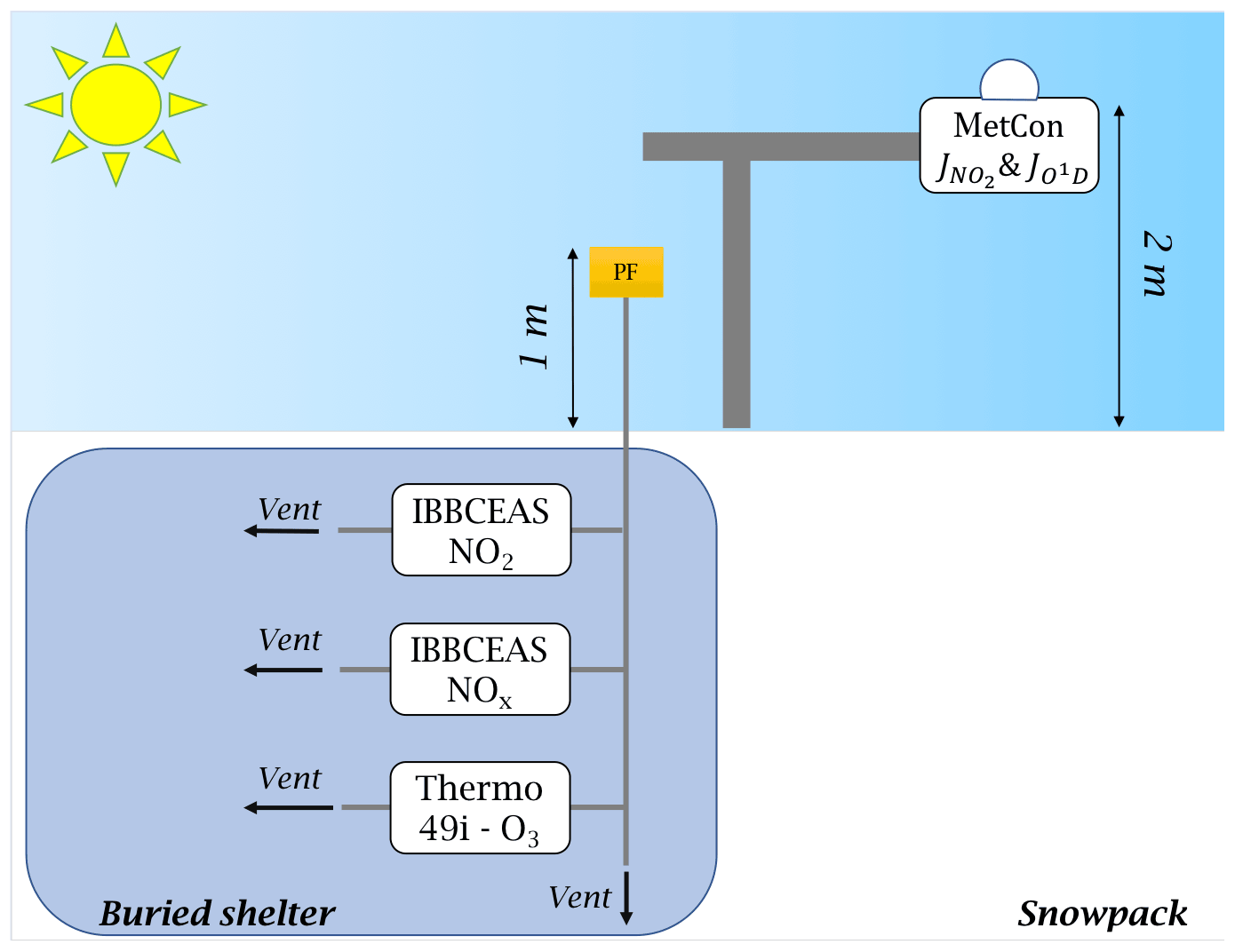
Figure 3 Set-up schematic. The photolysis rate constant of NO₂ and O¹D were measured by a 2π spectral radiometer (MetCon) placed 2 m above the snow surface; the atmospheric sampling of NO₂, NO_x, and O₃ was made 1 m above the snow surface through 0.25 in. PTFE tubing. Note that 5 µm particle filters (PFs) were placed at the inlets to protect the optics of the instruments' measuring cells.

2.2 Instrumentation and data processing

2.2.1 Measurement of atmospheric NO_x and O₃

The two instruments described in Barbero et al. (2020) were used for NO_x detection in the 400–475 nm wavelength region. These instruments are based on incoherent broadband cavity-enhanced absorption spectroscopy (IBBCEAS) with a high-power LED source injected in a high-finesse cavity (F≈33 100), with the transmission signal detected by a compact spectrometer equipped with a charge-coupled device (CCD) camera. Through this, we achieved direct detection of NO₂ with a detection limit of 30 pptv at 3σ precision with ≈20 min of signal integration. To indirectly measure NO, we installed a compact ozone generator (based on water electrolysis: 3 H₂O = 3 H₂ + O₃; reaction induced by hydrolysis cells Barbero et al., 2020) that converts all ambient NO into NO₂ via the reaction NO + O₃→ NO₂ + O₂. Additionally, the instrument configuration allows the spectrometer to operate at low temperature, making potential interferences from the thermal degradation of HO₂NO₂, for example, negligible (estimated at 1 pptv at 10 ^∘C). Furthermore, very limited NO₂ (0.001 pptv) is produced by the reaction of HONO + OH → NO₂ + H₂O, and less than 8 to 16 ppqv for 200 pptv of NO₂ is formed through the heterogenous reaction of NO₂ and H₂O (Finlayson-Pitts et al., 2003; Barbero et al., 2020). The possible interference due to NO₂, NO, or NO₃ should be limited because their rate constants are several orders of magnitudes lower than that for the NO oxidation. Finally, in the NO measurement mode, spectral interferences were studied, as small imperfections on the fit could lead to large effects on the NO₂ retrieved mixing ratio, particularly at sub-parts-per-billion levels. No substantial effects of potential artefacts were observed when O₃ mole fractions up to 8 ppmv were used, and applied O₃ mole fractions were kept below 6 ppmv (5.6 ± 1.5 and 4.3 ± 0.5 ppmv in December and January, respectively) during this field study. Ultimate detection limits of 33 and 63 pptv (3σ) for NO_x and NO (taking into account the propagation error), respectively, are also achieved within ≈20 min of measurement (Barbero et al., 2020), according to an Allan–Werle statistical method (Werle et al., 1993). The instruments were calibrated prior to and after field deployment using a stable reference NO₂ source (FlexStream™ Gas Standards Generator, KINTEK Analytical, Inc.), covering a large range of concentrations from the parts per trillion by volume to parts per billion by volume range (Barbero et al., 2020). In the field, a shorter time average of 10 min was used, which included the acquisition of the reference (I₀) and absorption (I) spectra. This shorter measurement still provides excellent detection limits of 54 and 48 pptv (3σ) for NO_x and NO₂, respectively, while providing a higher-resolution dataset that is more successful when removing possible polluted events from the dataset. Field calibrations were made using NO₂ and NO gas bottles (Air Liquide: 1 ppm NO₂ in N₂; Messer: 1 ppm NO in N₂) diluted with a zero-air flow for multi-point calibrations. Additionally, the NO₂ bottle was calibrated prior the field campaign against a laboratory standard. The zero-air flow was produced by pumping outdoor air through two zero-air cartridges connected in series (TEKRAN 90-25360-00 Analyzer Zero Air Filter) and controlled by two mass flow controllers (MKS mass flow controller at 0.01 and 10 standard litres per minute, slpm, 1 splm = $\mathrm{1.6667}\times {\mathrm{10}}^{-\mathrm{5}}$ m³ s⁻¹, for the NO₂ flow and the zero-air flow, respectively). The NO_x measurements from the IBBCEAS were synchronized in time for a more accurate estimate of the NO mixing ratio (NO = NO_x − NO₂). To limit the impact of variable weather and atmospheric conditions on NO₂ and NO observations and approximate a steady state to use Leighton's relationship (Leighton, 1961), we restricted data to when the wind was between 135 and 338^∘ (i.e. not coming from the direction of the station) with a speed below 5 m s⁻¹. These constraints resulted in 17 % rejection rate for the first observation period and 11 % for the second period. During the second period, approximately 4 d of measurements were further rejected because the instruments were used for intercomparison and calibration purpose. After this quality control, the accepted data were aggregated to hourly means in order to improve the signal to noise ratio. Atmospheric ozone was monitored using a UV Photometric O₃ analyser (Thermo Scientific™, Model 49i) that has a 1.5 ppbv (3σ) detection limit for 60 s data. The instrument was calibrated on site with an O₃ calibration source (2B Technologies Model 306 Ozone Calibration Source™) and connected to an existing air sampling tower at 1 m above the snow surface (Helmig et al., 2020) (Appendix C). Here, samples were drawn sequentially at typical flows of ≈ 1–2 slpm through a series of switching valves connected to several inlet lines, following a 2 h duty cycle of 8 min measurements on each inlet. To account for the switching manifold response time, only the last 3 min of measurements of steady-state concentrations were used and averaged, giving one measurement of ozone mixing ratio every 2 h. A linear data interpolation on the O₃ measurements was applied to match the resolution of the NO_x and NO₂ measurements. Particle filters (Whatman™ PTFE membrane filters TE 38, 5 µm, 47 mm) were placed in the inlet lines (IBBCEAS and Thermo 49i) for removing aerosol particles.

Figure 4 $J_{{\mathrm{NO}}_{\mathrm{2}}}$ (solid blue lines) reconstruction following the 2^∘ polynomial regression fit (shown in Appendix D) with UV radiation (shaded red) measured by a broadband UV radiometer (spectral range 305–385 nm) for both the December (a) and January (b) observation periods.

2.2.2 Ancillary data

Standard meteorological data were collected from an automatic weather station (AWS) located 1 km away from the atmospheric measurements (Fig. 2). The UV radiation spectrum was analysed with a broadband UV radiometer (Kipp & Zonen CUV 4, spectral range 305–385 nm) deployed near the air clean sector.

2.2.3 The photolysis rate coefficients $J_{{\mathrm{NO}}_{\mathrm{2}}}$ and $J_{{\mathrm{O}}^{\mathrm{1}}\mathrm{D}}$

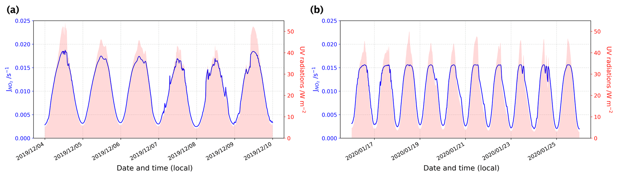
The photolysis rate coefficients, $J_{{\mathrm{NO}}_{\mathrm{2}}}$ and $J_{{\mathrm{O}}^{\mathrm{1}}\mathrm{D}}$, were calculated from measurements made by a MetCon 2π spectral radiometer with a charge-coupled device. The spectral radiometer was mounted on a mast at 2 m from the snow surface (Fig. 3), and downwelling radiance was recorded over the full spectral range of the radiometer from 285 to 700 nm. Unfortunately, unstable power supply issues resulted in irregular operation during the summer campaign, particularly during local night-time hours, and a continuous signal was reconstructed using the broadband UV radiometer to scale the data from the 2π spectral radiometer. Later, the total 4π steradian radiance was calculated by multiplying the measurements by 1.9, as this factor was determined from downwelling and upwelling radiance measurements during the OPALE campaign (Kukui et al., 2014). The estimated $J_{{\mathrm{NO}}_{\mathrm{2}}}$ for both measurement periods is shown in Fig. 4, and details on the fit analysis are provided in Appendix D. Due to the intermittent measurements, differences between the fit analysis and the $J_{{\mathrm{NO}}_{\mathrm{2}}}$ measurements were found to be around 0.8 ± 4.7 % (1σ) in December and 3.6 ± 5.4 % (1σ) in January. These extrapolations agree well with previous measurements done during the 2011–2012 OPALE campaign using the same 2π spectral radiometer. Kukui et al. (2014) found a median value of $J_{{\mathrm{NO}}_{\mathrm{2}}}$ = 1.3 × 10⁻² s⁻¹ (0.4 to 2.1) from 19 December 2011 to 10 January 2012, very close to the one found in this work for the same period: 1.3 × 10⁻² s⁻¹ (0.3 × 10⁻² to 2.9 × 10⁻² s⁻¹). In a similar manner, we calculated $J_{{\mathrm{O}}^{\mathrm{1}}\mathrm{D}}$ (median value of 1.2 × 10⁻⁵ s⁻¹, range 0.1 × 10⁻⁵ to 5.1 × 10⁻⁵ s⁻¹) from the UV radiation data (please refer to Appendix D for more information).

2.3 NO₂:NO ratio analysis

At steady state, the relationship between the reactions NO + O₃ and NO₂ photolysis, known as the simple Leighton's relationship (Leighton, 1961), can be described by Eq. (1):

$$\begin{array}{}\text{(1)}& {\mathrm{NO}}_{\mathrm{2}}:\mathrm{NO}={\displaystyle \frac{k_{\mathrm{NO}+{\mathrm{O}}_{\mathrm{3}}}\left[{\mathrm{O}}_{\mathrm{3}}\right]}{J_{{\mathrm{NO}}_{\mathrm{2}}}}},\end{array}$$

where [O₃] is the ozone concentration (in molec. cm⁻³), $k_{\mathrm{NO}+{\mathrm{O}}_{\mathrm{3}}}=\mathrm{1.4}$ × 10${}^{-\mathrm{12}}\exp \left(\frac{-\mathrm{10.89}}{\mathrm{RT}}\right)$ is the constant rate of the reaction NO + O₃ (Atkinson et al., 2004) (in cm³ molec.⁻¹ s⁻¹), and $J_{{\mathrm{NO}}_{\mathrm{2}}}$ is the NO₂ photolysis rate constant (in s⁻¹), measured with the MetCon instrument and reconstructed as explained in Sect. 2.2.3. However, as illustrated in Fig. 1, the simple Leighton's relationship can be perturbed by other species such as peroxy radicals and halogenated radicals. Therefore, the NO₂:NO ratio can also be calculated from an extended Leighton mechanism also including peroxy radicals as described in Eq. (2) (Ridley et al., 2000):

$$\begin{array}{}\text{(2)}& {\mathrm{NO}}_{\mathrm{2}}:\mathrm{NO}={\displaystyle \frac{k_{\mathrm{NO}+{\mathrm{O}}_{\mathrm{3}}}\left[{\mathrm{O}}_{\mathrm{3}}\right]+\sum k_{\mathrm{NO}+{\mathrm{RO}}_x}\left[{\mathrm{RO}}_x\right]}{J_{{\mathrm{NO}}_{\mathrm{2}}}}}.\end{array}$$

Kukui et al. (2014) measured the RO_x at Dome C during the OPALE campaign at 1 m above the snow surface. They assumed that HO₂ and CH₃O₂ radicals represent the major part of all RO₂ radicals at Dome C, with a ratio of HO₂:RO₂ = 0.67 ± 0.05. Additionally, Kukui et al. (2014) found a linear correlation between the $J_{{\mathrm{NO}}_{\mathrm{2}}}$, measured with the same MetCon instrument, and the concentrations of RO₂ (see Fig. 3 of their study). Here, we used the same correlation and the ratio of 0.67 to estimate RO₂ and HO₂ atmospheric concentrations, respectively (more information can be found in Appendix E). The reactions between those dominating peroxy radicals, RO₂ and HO₂, and nitrogen oxide are rapid with respect to NO + O₃, with mean rate coefficients of (1.10 ± 0.02) × 10⁻¹¹ and (0.91 ± 0.02) × 10⁻¹¹ cm³ molec.⁻¹ s⁻¹, respectively, while $k_{\mathrm{NO}+{\mathrm{O}}_{\mathrm{3}}}$ = (6.35 ± 0.53) × 10⁻¹⁵ cm³ molec.⁻¹ s⁻¹ in Dome C daily conditions. Therefore, Eq. (3) is used to consider those reactions and calculate NO₂:NO ratios from O₃ in situ measurements and RO_x observations taken from Kukui et al. (2014).

$$\begin{array}{}\text{(3)}& \begin{array}{rl}& {\mathrm{NO}}_{\mathrm{2}}:\mathrm{NO}=\\ & {\displaystyle \frac{k_{\mathrm{NO}+{\mathrm{O}}_{\mathrm{3}}}\left[{\mathrm{O}}_{\mathrm{3}}\right]+k_{\mathrm{NO}+{\mathrm{CH}}_{\mathrm{3}}{\mathrm{O}}_{\mathrm{2}}}\left[{\mathrm{CH}}_{\mathrm{3}}{\mathrm{O}}_{\mathrm{2}}\right]+k_{\mathrm{NO}+{\mathrm{HO}}_{\mathrm{2}}}\left[{\mathrm{HO}}_{\mathrm{2}}\right]}{J_{{\mathrm{NO}}_{\mathrm{2}}}}}\end{array}\end{array}$$

2.4 Atmospheric dynamic and polar boundary layer effect

In an attempt to decipher the mechanisms occurring at Dome C during our observation periods, we decided to account for the dilution effect due to the diurnal variation of the planetary boundary layer (PBL). To do so, in the second part of the results section, we referred our measurements to the total number of molecules using Eq. (4):

$$\begin{array}{}\text{(4)}& N_i=\left[i\right]\times V,\end{array}$$

where N_i is the total number of molecules of the species i (i = NO_x, NO, NO₂, HO₂, RO₂ and O₃), [i] is its concentration (expressed in molec. cm⁻³), and V is an arbitrary volume (expressed as 1 cm × 1 cm × H_PBL), with H_PBL as the boundary layer height in centimetres retrieved using the MAR regional model (see Appendix F for details). This calculation assumes a homogeneous concentration distribution of the species within the PBL, an assumption supported by the flat concentration profiles observed by Frey et al. (2015) and Legrand et al. (2016) within the PBL during the OPALE campaign, where O₃ and NO_x distribution are showing homogeneous mixing ratios within the entire polar boundary layer (PBL), except from 18:00 to 00:00 LT (local time) due to the collapse of the convective PBL.

3 Results

Both NO₂ and NO exhibited diurnal variations, with the highest concentrations in the afternoon and evening and lowest concentrations in the mid-morning to noon (Fig. 5), in association with the collapse and rise of the polar boundary layer (PBL) (Legrand et al., 2009; Frey et al., 2013, 2015). Generally, the rise and fall in NO₂ lagged behind the NO peak by 4–6 h. As a result, the NO₂:NO ratio had less diurnal amplitude than either NO₂ or NO. Overall, the mean NO₂:NO ratio was 1.3 ± 1.1 (1σ) for December and 0.4 ± 0.4 (1σ) for January. A possible reason for time lag are the different residence times in the porous snow after production, and transport through snow can indeed be slowed due to interaction with the snow interface, (Bartels-Rausch et al., 2013). However, both NO₂ and NO are not adsorbed by snow (Bartels et al., 2002). As explained in Sect. 2.3, RO₂ plays an important role in the oxidation. Therefore, RO₂ might be expected to be adsorbed to snow more than NO₂, similar to HNO₄ (Ulrich et al., 2012), and be released later.

The NO₂:NO ratios calculated from the extended and simple Leighton relationships (Eqs. 1, 3) share similar diurnal patterns to the observed NO₂:NO ratios but do not reflect the difference in mean value between December and January (Fig. 6). In December, the observed NO₂:NO is systematically higher than the one estimated using simple and extended Leighton's equilibrium (Fig. 6a), while in January it more closely matches the extended equilibrium estimations (Fig. 6b).

Figure 5 (top) The left-hand (dark blue) scale shows the mixing ratios (pptv) of NO₂ (blue), NO (black), and NO_x (cyan), and the right-hand (red) scale shows the NO₂:NO ratio. (bottom) The left-hand (green) scale shows the mixing ratio of O₃ (ppbv), and the right-hand (orange) scale shows UV radiation (W m⁻²) measured with a broadband radiometer in the spectral range 305–385 nm. The signals are 6 h running means (solid) on top of 1 h mean signals (dashed). Each day is marked with vertical black lines at 00:00 LT.

We observed a dramatic loss of O₃ at the end of the measurement period, with the mean mixing ratio dropping from 29.8 ± 3.6 ppbv during 16–20 January to 14.3 ± 0.8 ppbv during 23–25 January. HYSPLIT 5 d backward trajectories between 14:00 and 20:00 LT on 23 January (Appendix A2) reveal that the air mass over Dome C originated from the east coast of Antarctica, and this could explain the 10 ppbv drop of O₃ observed between the two January periods shown in Fig. 5. It is therefore possible that this air mass was partially affected by marine influences, as Legrand et al. (2009, 2016) concluded that O₃ mixing ratios below 20 ppbv were observed when the air masses spent at least 1 d above the ocean during the previous 5 d. As a result, we excluded the 23–25 January data from the following discussions. Figure 7a and b show the daily averaged total number of molecules (Eq. 4) of $N_{{\mathrm{NO}}_x}$ (cyan), N_NO (black), and $N_{{\mathrm{NO}}_{\mathrm{2}}}$ (blue) for both observation periods, December 2019 (Fig. 7a) and January 2020 (Fig. 7b). The total number of molecules is used to cancel the PBL dynamic, as explained in Sect. 2.4. The NO₂:NO ratios observed (red) in comparison with the theoretical NO₂:NO calculated from Eq. (1) (NO₂:NO)_sim in grey and Eq. (3) (NO₂:NO)_ext in black are reported in the lower panels of Fig. 7a and b. With the objective of testing the consistency of the observed NO₂:NO ratios with ozone production and destruction, in Fig. 7c and d we also reported the total number of O₃ molecules in a column of 1 cm × 1 cm × 1 H_PBL cm (green, left-hand scale), with its variation over time, i.e. $\frac{{\mathrm{d}}_{{\mathrm{O}}_{\mathrm{3}}}}{\mathrm{d}t}$ (in molec. h⁻¹, blue-grey, right-hand scale). Production of ozone, $P_{{\mathrm{O}}_{\mathrm{3}}}$ (expressed in molec. h⁻¹), calculated as the NO₂ production rate from the reactions RO₂ + NO → NO₂ + RO and HO₂ + NO → NO₂ + OH, as reported by Kukui et al. (2014), is calculated following Eq. (5) and reported in violet in Fig. 7c and d.

$$\begin{array}{}\text{(5)}& P_{{\mathrm{O}}_{\mathrm{3}}}=\left(k_{{\mathrm{RO}}_{\mathrm{2}}+\mathrm{NO}}\left[{\mathrm{RO}}_{\mathrm{2}}\right]+k_{{\mathrm{HO}}_{\mathrm{2}}+\mathrm{NO}}\left[{\mathrm{HO}}_{\mathrm{2}}\right]\right)\times \left[\mathrm{NO}\right]\times V\end{array}$$

In the above equation, $k_{{\mathrm{RO}}_{\mathrm{2}}+\mathrm{NO}}$ and $k_{{\mathrm{HO}}_{\mathrm{2}}+\mathrm{NO}}$ are the kinetic rate coefficients of the reactions RO₂ + NO → NO₂ + RO and HO₂ + NO → NO₂ + OH, respectively (expressed in cm³ molec.⁻¹ s⁻¹); [RO₂] and [HO₂] are the species concentrations (expressed in molec. cm⁻³) and are derived from the correlation between $J_{{\mathrm{NO}}_{\mathrm{2}}}$ and [RO₂] and the $\frac{\left[{\mathrm{RO}}_{\mathrm{2}}\right]}{\left[{\mathrm{HO}}_{\mathrm{2}}\right]}$ ratio (Kukui et al., 2014); [NO] is the concentration of NO (expressed in molec. cm⁻³); and V the arbitrary volume (expressed as 1 cm × 1cm × H_PBL cm, with H_PBL given by the MAR regional model; see Appendix F for details). The overall daily mean $\frac{P_{{\mathrm{O}}_{\mathrm{3}}}}{V}$ calculated for this study (≈ 0.22 ppbv h⁻¹) is close to the 0.3 ppbv h⁻¹ calculated by Kukui et al. (2014) and the 0.2 ppbv h⁻¹ derived from the study of the ozone diurnal concentration by Legrand et al. (2009). In Fig. 7c and d, the deviations of the observed ratio (NO₂:NO)_obs from the simple and extended Leighton's equilibria are reported, i.e. Δ_sim(NO₂:NO) = (NO₂:NO)_obs − (NO₂:NO)_sim and Δ_ext(NO₂:NO) = (NO₂:NO)_obs − (NO₂:NO)_ext for each period, respectively. Looking at Fig. 7a and b, the NO_x, NO, and NO₂ peaks are now more in phase with the variability of the UV radiation. The total number of NO molecules and their diurnal variability appear constant from December to January, with a maximum from 11:00 to 17:00 LT. NO₂ shows a similar trend in December with a maximum from 10:00 to 18:00 LT, while in January the total number of NO₂ molecules in the atmospheric boundary layer is somewhat constant during the day, with a slight increase from 09:00 to 12:00 LT.

Figure 6 NO₂:NO ratios measured (red) and estimated from Eqs. (1) (blue) and (3) (black) for both observation periods: December (a) and January (b). Solid lines represent the 6 h running mean smoothed signals.

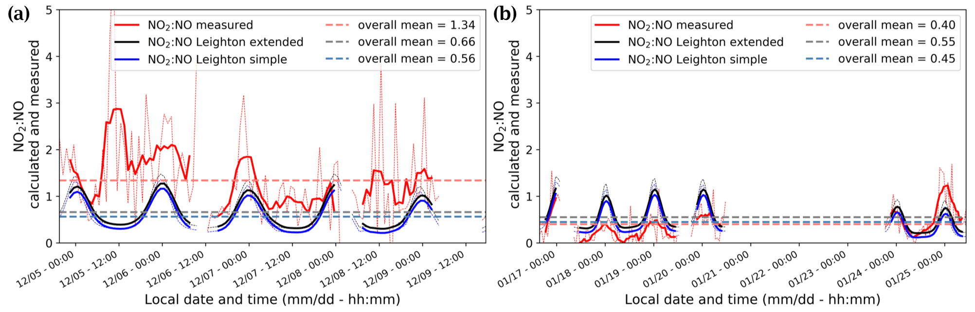
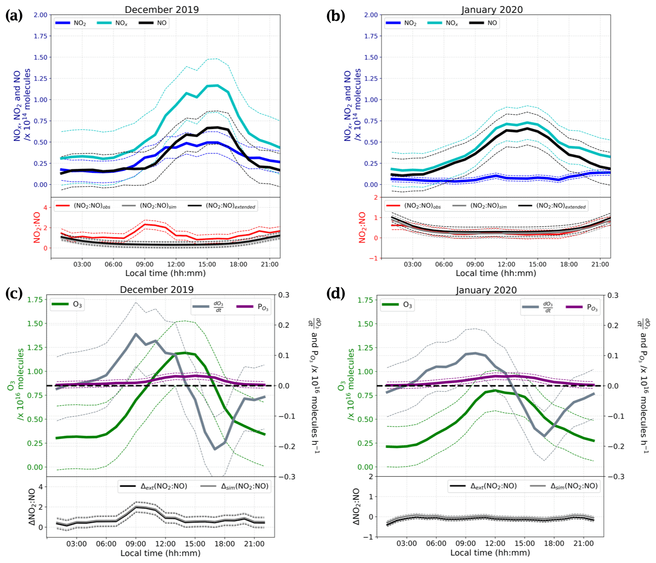
Figure 7 The top part of panels (a) and (b) show the diurnal cycles of the total number of molecules in a column of 1 cm × 1 cm × 1 H_PBL cm for the of NO (black), NO_x (cyan), and NO₂ (blue). The bottom parts of these panels show the NO₂:NO ratios observed (red) and equilibrium's calculations (simple Leighton in grey and extended Leighton in black) for December and January, respectively. The solid lines represent the 3 h running mean ±1σ (thin dashed lines). The top part of panels (c) and (d) represent the diurnal cycle of the total number of ozone molecules in a column of 1 cm × 1 cm × 1 H_PBL cm (green), the O₃ variations, $\frac{d_{{\mathrm{O}}_{\mathrm{3}}}}{\mathrm{d}t}$ (in molec. h⁻¹, grey) and the ozone production, $P_{{\mathrm{O}}_{\mathrm{3}}}$ (in molec. h⁻¹, violet) calculated from the total number of RO₂ and NO molecules. The bottom parts of these panels represent the differences between observed NO₂:NO and calculated NO₂:NO; Δ_sim(NO₂:NO) is shown in grey for simple Leighton, and Δ_ext(NO₂:NO) is shown in black for extended Leighton. The solid lines represent the 3 h running mean ±1σ (thin dashed lines).​​​​​​​

4 Discussion

4.1 What is driving the observed patterns?

From Fig. 7, it appears that in December the NO₂:NO is above the NO₂:NO predicted by Leighton's equilibria (both simple and extended), with a peak in the morning from 07:00 to 12:00 LT, but approaches equilibrium from noon onwards, inversely following the ozone signal (Fig. 7). In January, it follows the equilibrium quite well, except during night-time, when it is approximately half the predicted value calculated at steady state. The O₃ variations measured in our study $\frac{{\mathrm{d}}_{{\mathrm{O}}_{\mathrm{3}}}}{\mathrm{d}t}$ show significant differences with the ozone production $P_{{\mathrm{O}}_{\mathrm{3}}}$ calculated using RO₂, HO₂, and NO concentrations. $P_{{\mathrm{O}}_{\mathrm{3}}}$ from Fig. 7c and d shows not only a factor of 10 difference with the O₃ daily variations but also a rather different behaviour. Indeed, using RO₂, HO₂, and NO concentrations, O₃ appears to be gradually produced, following the UV radiation, with a maximum production in the afternoon, from approximately 12:00 to 16:00 LT. However, this calculated production is largely insufficient to explain the observed variability of O₃. Observations show ozone production, (i.e. values above the dashed bold black line in Fig. 7), from around 02:00 to 14:00 LT, with the maximum reached at 11:00 (local solar noon), and destruction of ozone (i.e. values under the dashed black line in Fig. 7), from 14:00 to midnight (LT), with the maximum consumption around 17:00–18:00 LT. While Legrand et al. (2009) attributed this behaviour to the variability of the PBL, here its impact is accounted for through the observation of a total number of molecules in a column within the boundary layer height. Therefore, the dynamic of the PBL is not the only explanation for the O₃ variability. Even though the deviation Δ(NO₂:NO) from Leighton's equilibria is always positive, at those levels of O₃ a deviation of Δ(NO₂:NO) = 0.5 from steady state might not be enough to maintain an O₃ production (Fig. 7c). Additionally, the Δ(NO₂:NO) peak in December is slightly shifted with respect to the $\frac{{\mathrm{d}}_{{\mathrm{O}}_{\mathrm{3}}}}{\mathrm{d}t}$ (Fig. 7c). This shift is explained by the chemical lifetime of the species. NO₂ lifetime, ${\mathit{\tau }}_{{\mathrm{NO}}_{\mathrm{2}}}$ = $\frac{\mathrm{1}}{J_{{\mathrm{NO}}_{\mathrm{2}}}}$, varies from ≈ 6 min at 00:00 LT to ≈ 1 min at 11:00 LT, largely inferior to O₃ chemical lifetime. Legrand et al. (2016) show that the main sink of O₃ is the HO₂ radical, and it is therefore driving its lifetime: ${\mathit{\tau }}_{{\mathrm{O}}_{\mathrm{3}}}$ = $\frac{\mathrm{1}}{k_{{\mathrm{HO}}_{\mathrm{2}}+\mathrm{NO}}\left[{\mathrm{HO}}_{\mathrm{2}}\right]}$ varies from ≈ 2 years at 00:00 LT to ≈ 0.4 year at 11:00 LT. However, the O₃ dry deposition was not considered in the $P_{{\mathrm{O}}_{\mathrm{3}}}$ calculation. The NO₂:NO ratio seems to follow Leighton's equilibrium in January, and since the NO trend remains the same between the two observation periods, it highlights the necessity of an additional primary source of NO₂ other than the conversion of NO to NO₂ by reactions with O₃ and radicals, as shown in Fig. 1. Additionally, in January the seemingly extended Leighton's equilibrium cannot explain the O₃ loss observed from the $\frac{{\mathrm{d}}_{{\mathrm{O}}_{\mathrm{3}}}}{\mathrm{d}t}$ signal. The chemical lifetime of O₃ with respect to its photolysis (${\mathit{\tau }}_{{\mathrm{O}}_{\mathrm{3}}}$ = $\frac{\mathrm{1}}{J_{{\mathrm{O}}^{\mathrm{1}}\mathrm{D}}}$, with $J_{{\mathrm{O}}^{\mathrm{1}}\mathrm{D}}$ reconstructed from the MetCon instrument) is estimated to range from 7 h to several days. Another sink of O₃ with a chemical lifetime closer to ${\mathit{\tau }}_{{\mathrm{NO}}_{\mathrm{2}}}$ is necessary to explain the O₃ loss observed for both periods. In an attempt to explain the large NO₂ excess observed at maximum sunlight in December, the NO_x snow source is studied in light of the conclusions given in Barbero et al. (2021), where flux chamber experiments carried out from 10 December to 7 January during the 2019–2020 campaign at Dome C, Antarctica, suggested that the photolysable nitrate present in the snow acts as a uniform source with similar photochemical characteristics, and a robust average daily photolysis rate coefficient $J_{{\mathrm{NO}}_{\mathrm{3}}^{-}}$ of (2.37 ± 0.35) ×  10⁻⁸ s⁻¹ (1σ) was estimated for the Antarctic Plateau photic zone (0–50 cm layer).

Table 1 NO, NO₂, and NO_x mixing ratios (pptv) and NO₂:NO ratios measured at Dome C during this campaign, in comparison with previous NITEDC and OPALE campaigns for similar periods (period averages).

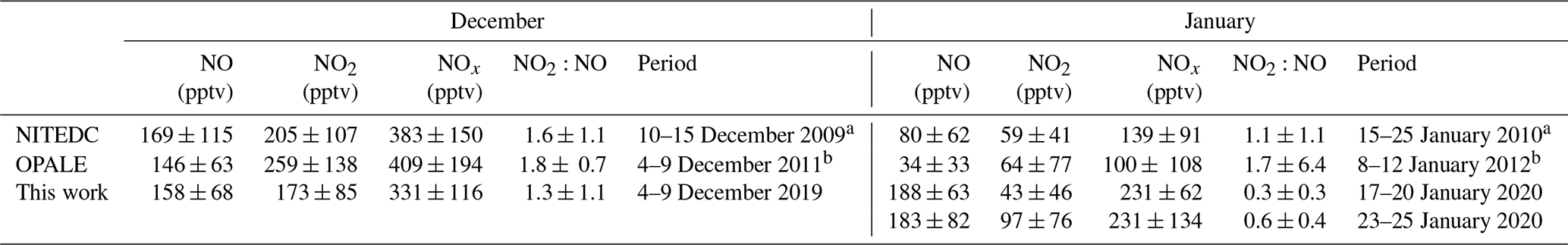
^a From Frey et al. (2013). ^b From Frey (2021).

4.2 Comparison with previous studies

Previous studies as part of the NITEDC and OPALE missions estimated the NO₂:NO ratio at Dome C on the East Antarctic Plateau, and we can compare these estimates to our field-observed data (Table 1). In this work, an average mixing ratio of 158 ± 68 pptv (1σ) was measured for NO during the December observation period, which is similar to the mixing ratios of 169 ± 115 and 146 ± 63 pptv reported from the NITEDC and OPALE campaigns for a similar period (Frey et al., 2013, 2015). However, levels of NO_x and NO₂ from NITEDC and OPALE were ≈ 30 % greater than that measured in this study (Table 1), and their NO₂:NO ratios are similarly greater than our ratio as a result. For January, we found an average NO mixing ratio of 188 ± 63 pptv (1σ), and this is almost 2.5 times what Frey et al. (2013) measured (80 ± 62 pptv) in January 2010. Moreover, during the OPALE campaign, Frey et al. (2015) measured ≈ 6 times less NO but similar NO₂ mixing ratios, leading to a high NO₂:NO of 1.7 ± 6.4 relative to our ratio of 0.3 ± 0.3. The NITEDC results suggested that either an unknown process enhancing NO₂ was taking place at Dome C or that peroxy and other radicals would be significantly higher than elsewhere in Antarctica.

While differences in atmospheric dynamics and snow cover during the different campaigns could explain the discrepancy observed in December and January, where “atmospheric composition above the East Antarctic plateau depends not only on atmospheric mixing but also critically on NO${}_{\mathrm{3}}^{-}$ concentration and availability to photolysis in surface snow as well as incident UV irradiance”, as explained in Frey et al. (2015), it may also be due to different detection techniques being used. For NITEDC and OPALE (Frey et al., 2013, 2015), NO_x was measured with a two-channel chemiluminescence detector (CLD), based on the reaction of NO with excess O₃ to produce NO₂. One channel was dedicated to NO and the other to NO_x; atmospheric NO₂ concentrations were then calculated as the signal difference between those two channels (Bauguitte et al., 2012). In our study, NO₂ is measured directly by the IBBCEAS. However, the NO measurement is made indirectly through the detection of NO_x after quantitative conversion of all ambient NO to NO₂ via NO + O₃ → NO₂ + O₂; in a way, this is the opposite of what is done in the CLD technique. The possible interferences on NO₂ measurements from the presence of high O₃ levels are discussed in Barbero et al. (2020), as several reactions could be triggered at elevated O₃ concentrations, as discussed in Sect. 2.2.1. The discrepancies observed between the IBBCEAS measurements and the previous CLD measurements could be explained by positive and negative interferences on the CLD technique. Indeed, the indirect measurement of NO₂ by the CLD may suffer from interferences due to the presence of other gaseous species, such as HONO and HO₂NO₂, in the inlet lines, which will be then photolytically converted. Reed et al. (2016) suggested that measurements of NO₂ using CLD systems may be significantly biased in low-NO_x environments, especially in pristine environments, such as Dome C, where the NO_y to NO_x ratio may be high. The thermal decomposition of NO_x species within the NO₂ converter can produce unreasonably high measurements. Additionally, the photolytic conversion unit of the CLD instrument used in previous campaigns was at 30 ^∘C; therefore, the thermal decomposition of HO₂NO₂ could indeed be an important source of interference. Frey et al. (2013, 2015) discussed this possible interference and estimated it to be 8 %–16 % of the average NO₂ measurement at 1 m from the snowpack. This interference might indeed partially explain the higher NO₂:NO ratio observed during previous campaigns in respect to our study.

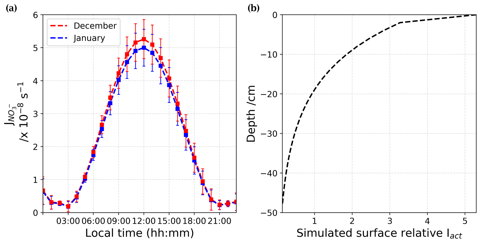
Figure 8 (a) Adjusted $J_{{\mathrm{NO}}_{\mathrm{3}}^{-}}$ (in s⁻¹) from December (red) and January (blue) estimated from Barbero et al. (2021) results. (b) Mean surface relative actinic flux, I_act, profile at 305 nm, calculated using the TARTES model (Libois et al., 2013, 2014). The actinic flux describes the number of photons that are incident at a point.

4.3 Presence of halogenated radicals

During the OPALE campaign, bromine oxide (BrO) column amounts were measured using a ground base UV–visible spectrometer (MAX-DOAS, Roscoe et al., 2014). After a complex analysis of the spectra, Frey et al. (2015) estimated a BrO median daily value of 2–3 pptv near the surface at Dome C. Additionally, Schönhardt et al. (2012) observed via satellite the presence of BrO and IO over Antarctica. However, the monthly maps of IO vertical column amounts (Fig. 4 of the study) show the presence of IO in the Antarctic Plateau late in spring (September–October) of around 1.0 to 1.5 × 10¹² molec. cm⁻². In contrast, in summer they found a column amount of IO below the limit of detection, i.e. below 0.7 pptv once converting the column amount to volume mixing ratio (satellite observations averaged over six subsequent years, 2004–2009) (Schönhardt et al., 2008). Vertical concentrations of BrO were found to be similar between December and January, ranging from 6.0 × 10¹³ to 7.0 × 10¹³ molec. cm⁻² (Fig. 5 of the Schönhardt et al., 2012 study). To our knowledge, there are no reports of near-surface ClO measurement in Antarctica. The reactions NO + XO → NO₂ + X (X ≡ Br, I, or Cl) show very similar reaction rate coefficients. Therefore, we here consider an average of all halogenated radicals XO to have a daily average rate coefficient of (2.5 ± 0.4) × 10⁻¹¹ cm³ molec.⁻¹ s⁻¹, calculated as the average of the three daily average rate coefficients for the reactions with BrO, IO, and ClO. The necessary amount of XO to reach steady state in December was calculated following Eq. (6):

$$\begin{array}{}\text{(6)}& \begin{array}{rl}& {\mathrm{NO}}_{\mathrm{2}}:\mathrm{NO}=\\ & {\displaystyle \frac{\begin{array}{c}{k}_{\mathrm{NO}+{\mathrm{O}}_{\mathrm{3}}}\left[{\mathrm{O}}_{\mathrm{3}}\right]+k_{\mathrm{NO}+{\mathrm{HO}}_{\mathrm{2}}}\left[{\mathrm{HO}}_{\mathrm{2}}\right]+k_{\mathrm{NO}+{\mathrm{CH}}_{\mathrm{3}}{\mathrm{O}}_{\mathrm{2}}}\left[{\mathrm{CH}}_{\mathrm{3}}{\mathrm{O}}_{\mathrm{2}}\right]\\ +k_{\mathrm{NO}+\mathrm{XO}}\left[\mathrm{XO}\right]\end{array}}{J_{{\mathrm{NO}}_{\mathrm{2}}}}}\end{array},\end{array}$$

which is rearranged and simplified to Eq. (7):

$$\begin{array}{}\text{(7)}& \left[\mathrm{XO}\right]=\mathrm{\Delta }{\mathrm{NO}}_{\mathrm{2}}:\mathrm{NO}\left({\displaystyle \frac{J_{{\mathrm{NO}}_{\mathrm{2}}}}{k_{\mathrm{NO}+\mathrm{XO}}}}\right).\end{array}$$

Daily mean averages for XO of 17 pptv were estimated, with a peak of 64 pptv at 11:00 LT. If such high levels of XO were present, they would have been detected by Frey et al. (2015).​​​​​​​ MAX-DOAS results for XO are suspected to be mainly BrO at Dome C. In addition, such high levels of XO would induce a fast destruction of O₃, which was not observed either. Finally, NO levels should have been lower in December than in January. Therefore, the assumption of an additional conversion of NO to NO₂ through XO or RO_x seems insufficient to explain the observations, and only the increased production of NO₂ from primary sources of NO₂ by a factor of 2 may justify the NO₂ excess observed in December and not in January. In the following sections, the NO_x snow source is studied in the light of the conclusions of Barbero et al. (2021), where dynamic flux chamber experiments allowed for a new parameterization of the snow nitrate photolysis occurring at Dome C.

4.4 NO₂ snow source

In Barbero et al. (2021), results of dynamic flux chamber experiments deployed on the Antarctic Plateau at Dome C are presented. A nitrate daily average photolysis rate constant, $J_{{\mathrm{NO}}_{\mathrm{3}}^{-}}$ = (2.37 ± 0.35) × 10⁻⁸ s⁻¹, for all different snow samples (depth and location) of the Antarctic Plateau (from 10 December to 7 January) is estimated. In the light of this new estimate, the NO_x snow source is studied here to evaluate the NO_x fluxes, $F_{{\mathrm{NO}}_x}$, and the NO_x production rate, $P_{{\mathrm{NO}}_x}$, in December and January using Eq. (8):

$$\begin{array}{}\text{(8)}& F_{{\mathrm{NO}}_x}=\underset{z}{\overset{\mathrm{0}}{\int }}{J}_{{\mathrm{NO}}_{\mathrm{3}}^{-}}\left[{\mathrm{NO}}_{\mathrm{3}}^{-}\right]\mathrm{d}z,\end{array}$$

where [NO${}_{\mathrm{3}}^{-}$] is the concentration of nitrate (in molec. cm⁻³) of snow available in the photic zone, defined as $z=-\mathrm{50}$ cm (Erbland et al., 2013). The nitrate photolysis rate coefficients were adjusted for the SZA variations, and corrective factors of 0.987 and 0.938 were found for December and January, respectively. At maximum sunlight, the $J_{{\mathrm{NO}}_{\mathrm{3}}^{-}}$ is slightly lower in January than in December, as the greater SZA in January lowers the maximum peak of UV radiation (Fig. 8a). Figure 8b shows the mean surface relative actinic flux, I_act, profile over the photic zone extracted from the SBDART model (Libois et al., 2013, 2014) at 305 nm, which is the optimal wavelength for nitrate photolysis. The actinic flux, I_act, is the number of photons crossing the unit horizontal area per unit of time from any direction at a given wavelength (photons cm⁻² s⁻¹ nm⁻¹). Therefore, the attenuation of $J_{{\mathrm{NO}}_{\mathrm{3}}^{-}}$ in the photic zone is driven by the attenuation of the $I_{\mathrm{act}}(\mathit{\lambda },\mathit{\theta },z)$, as shown by Eq. (9):

$$\begin{array}{}\text{(9)}& J_{{\mathrm{NO}}_{\mathrm{3}}^{-}}\left(\mathit{\lambda }\right)=\underset{z}{\overset{\mathrm{0}}{\int }}{\mathit{\sigma }}_{{\mathrm{NO}}_{\mathrm{3}}^{-}}(\mathit{\lambda },T)\mathit{\varphi }(T,\mathrm{pH})I_{\mathrm{act}}(\mathit{\lambda },\mathit{\theta },z)\mathrm{d}z,\end{array}$$

where θ is the SZA, λ (in nm) is the wavelength, z (in m) is the snowpack's depth, ${\mathit{\sigma }}_{{\mathrm{NO}}_{\mathrm{3}}^{-}}(\mathit{\lambda },T)$ is the absorption cross section of nitrate, and ϕ(T,pH) and $I_{\mathrm{act}}(\mathit{\lambda },\mathit{\theta },z)$ are nitrate photolysis quantum yield and actinic flux, respectively.

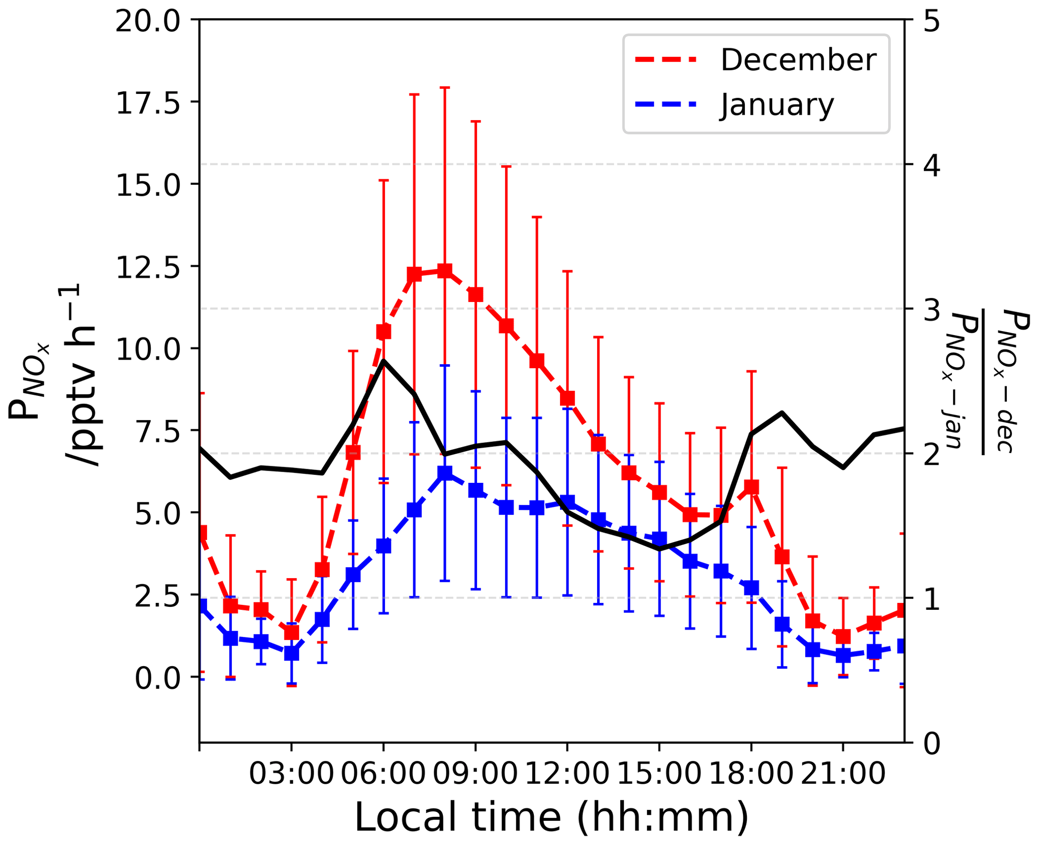
Figure 9 The left-hand scale shows the estimated $P_{{\mathrm{NO}}_x}$ (in pptv h⁻¹) in a column of 1 cm × 1 cm × H_PBL cm from December (red) and January (blue). The right-hand scale shows their ratio $\frac{P_{{\mathrm{NO}}_x\text{-Dec}}}{P_{{\mathrm{NO}}_x\text{-Jan}}}$ (unitless).

4.4.1 Surface snow

From Fig. 8b, one can see that I_act attenuates quickly with depth in the snowpack following an exponential decrease. Thus, the first few millimetres of the snow column dominate the availability of photons for photochemical reactions in the UV. Nitrate concentration measurements on surface snow were performed on a regular basis and for several years at Dome C (NITEDC and CAPOXI programmes). To reduce spatial and temporal variability, average surface concentration for periods corresponding to our atmospheric observations from samples taken at different locations in the clean area sector are used. The average nitrate concentration in surface snow (a few millimetres) is 991 ± 341 ppbw (parts per billion by weight or ng g⁻¹) (median 931–70 samples) in December and 588 ± 248 ppbw (median 558–65 samples) in January, respectively. This ≈ 40 % difference between December and January at the surface of the snowpack is significantly large. Considering Eq. (8)​​​​​​​ with a negligible dz for surface snow samples, we estimated the NO_x fluxes (expressed in molec. cm⁻² s⁻¹) from the snow surface source and converted it into a production rate (in molec. cm⁻³ h⁻¹) using the PBL height (cm). This production was then converted (into pptv h⁻¹) using atmospheric pressure, P (in hPa), and temperature, T (in K). Additionally, the mean surface relative I_act profile shows an enhancement of the actinic flux in the very first millimetre of snow (Fig. 8b); therefore, we multiplied the results by an enhancement factor of 5. Figure 9 illustrates the estimated $P_{{\mathrm{NO}}_x}$ (in pptv h⁻¹) from the surface snow for both periods. Because of the difference in nitrate in the surface snow, we estimated a mean ratio of 1.92 ± 0.33 in the NO_x production between December and January (Fig. 9, black curve on the right-hand scale). It is worth noting that a factor of up to 2.6 difference in the surface snow NO_x production between December and January could be reached in the early morning. Therefore, the snow source seems to be a good direction to explore. Indeed, in December, twice as much NO_x is produced by the snowpack in the morning, suggesting a more productive snowpack in December than in January, which could actually explain the deviation from the photochemical equilibrium in the morning.

4.4.2 Snowpack

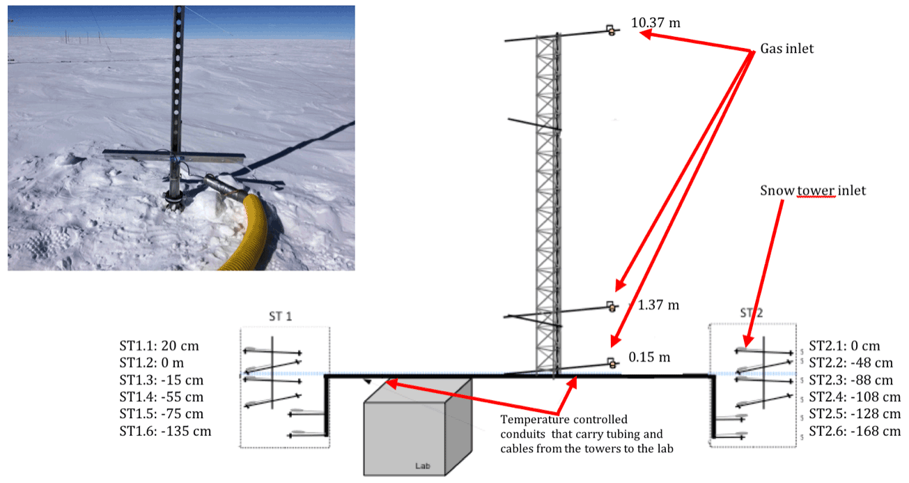
An automatic snow tower experiment (Helmig et al., 2020) allows for continuous year-round NO_x and O₃ measurements at different snow depths and heights above the snow surface, and this monitoring has been maintained since 2015 at the same location as our atmospheric observations (more information is provided in Appendix C). However, due to technical problems with the NO_x analyser during the 2019–2020 campaign, only the O₃ monitoring instrument was running. Figure 10 shows averaged 24 h NO_x mixing ratios in the interstitial air at −48 cm recorded in 2016–2017 for similar periods of time.

One can see that the NO_x measured at −48 cm, the bottom part of the photic zone, is ≈ 50 % times higher in December 2016 than in January 2017, strengthening the theory of a strong variability in the NO_x snow source during the photolytic season, with a depleted NO_x reservoir toward the end of the light season. It is worth noting that the NO${}_{\mathrm{3}}^{-}$ profiles are similar between the two seasons. Additionally, calculations based on the flux chamber (FC) results are probably underestimating the actual NO_x snow source, as mentioned in Barbero et al. (2021). Indeed, as discussed in Frey et al. (2013), the observed night-time increase in wind shear at Dome C (Fig. 2) likely causes enhanced upward ventilation of NO_x that temporarily accumulated in the upper snow pack during very stable conditions. This analysis strengthens the hypothesis of an enhanced NO₂ snow source in December, when the additional NO₂ flux seems sufficient to explain the NO₂ surplus.

However, additional investigations into possible unidentified mechanisms or sinks of O₃ are needed. Indeed, if the NO_x snow source might explain the differences between December and January in the NO_x cycle, this does not support the observed O₃ variations. Halogenated radicals, such as iodine (IO) and bromine (BrO), probably play their part; however, they are not significantly observed on the nitrogen oxide signal, but they possibly explain the behaviour of the ozone signal. Indeed, very recently Spolaor et al. (2021) observed a continuous decline since the 1970s in the iodine concentration in ice core samples from inner Antarctica. The study states that the enhanced UV radiation caused by the stratospheric ozone hole results in the increase of iodine re-emissions from the snowpack. This ice-to-atmosphere iodine mass transfer could indeed explain the ozone behaviour observed in the work presented here, as iodine catalytic cycles play a crucial role in the destruction of tropospheric ozone.

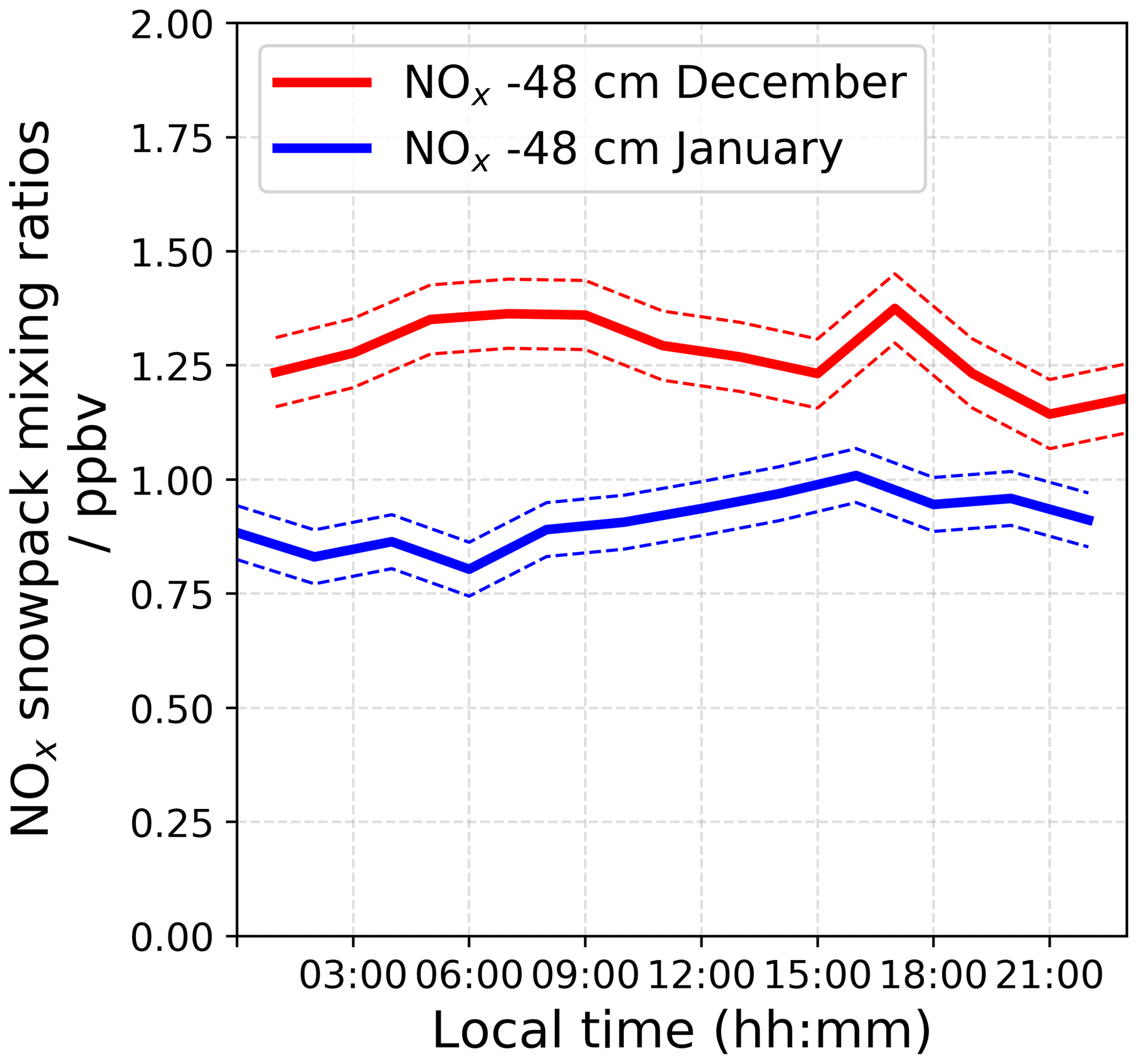
Figure 10 Averaged 24 h NO_x mixing ratios measured in the interstitial air at −48 cm by the automatic snow tower experiment in 2016–2017 for similar periods as our atmospheric observations.

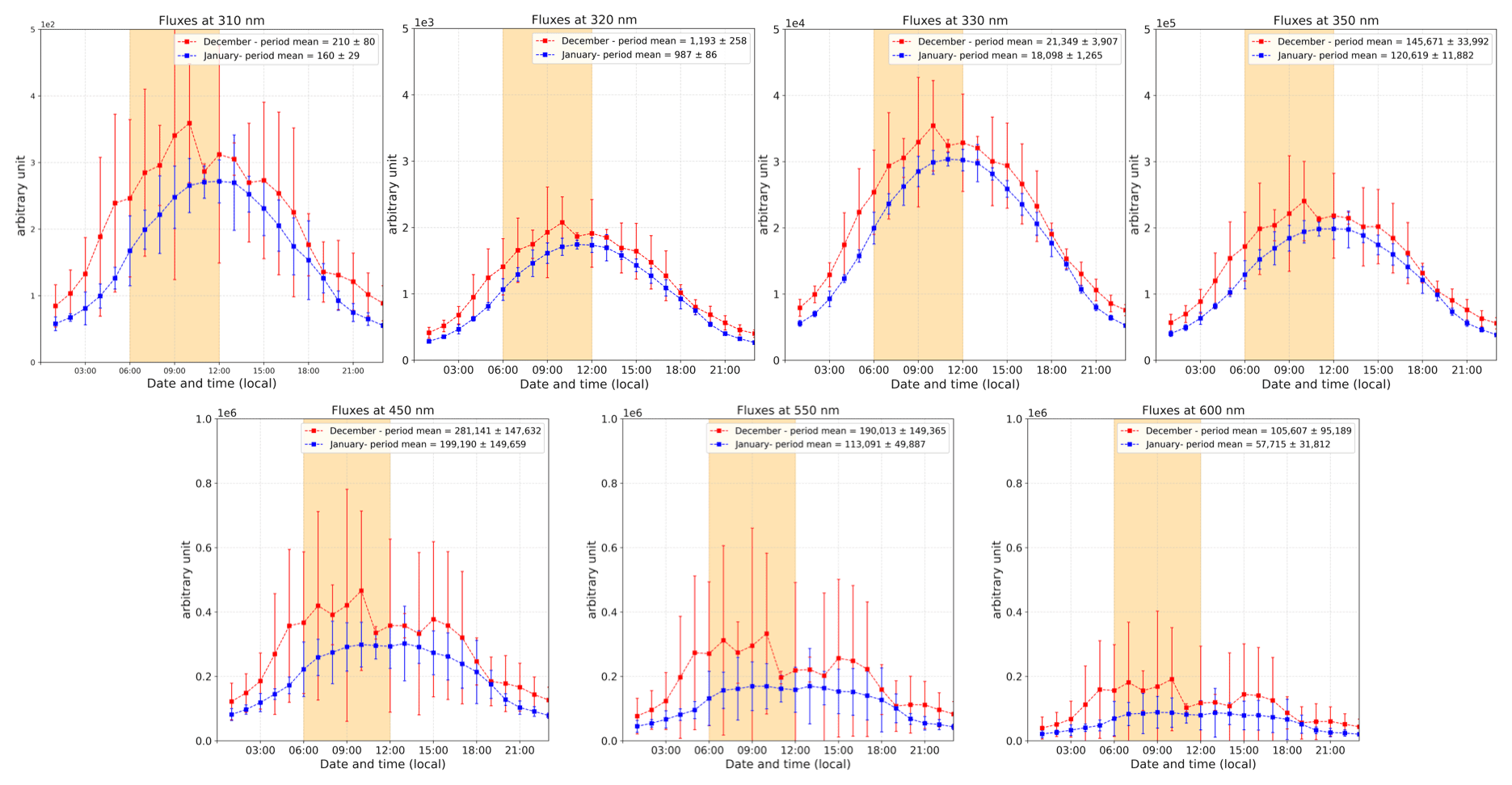
Figure 11 The 2 h running ±1σ (error bars) of the period-averaged diurnal cycles of relative radiation fluxes at different wavelengths (310, 320, 330, 350, 450, 550, and 600 nm) for both periods (December and January). The yellow-shaded area corresponds to the period where the NO₂:NO ratio is deviating from the steady-state equilibrium in December.

5 High sensitivity of the NO₂:NO ratio to the sun's position

A possible reason for this productivity of the snowpack in the morning during the earlier phase of the photolysis season is the number of photons available, leading to higher rate of photolysis in December. Nitrate photolysis in snow occurs for wavelengths λ>300 nm (305 nm being the optimal wavelength). Measurements of solar UV spectral radiation have been continuously recorded at Concordia since 2007 as part of the Network for the Detection of Atmospheric Composition Change (NDACC). The instrument, SAOZ (Système d'Analyse par Observation Zenithal), is an UV–visible (310–650 nm) diode array spectrometer (1 nm resolution), looking at the scattered sunlight (Pommereau and Goutail, 1988; Kuttippurath et al., 2010).

Figure 11 shows the relative radiation fluxes at different wavelengths in arbitrary units. One can see that the relative radiation flux is systematically higher in December than in January, which could be expected as 18 d separates the first observation period from the summer solstice versus 27 d for the second period. While this explains higher levels of NO_x due to more photolysis activity in the snowpack in December than in January, it does not explain the early morning excess. Indeed, one can see in Fig. 11 that the diurnal cycle of the radiation is somewhat symmetrical in January (in blue), while an asymmetry appears in December (in red). This is also visible while comparing the shape of the SZA for the two periods, with the difference between the two SZA cycles (black line in Fig. 12) showing a bump in the morning between 06:00 and 12:00 LT with a similar shape as the NO₂:NO deviation from equilibrium reported in Fig. 7a. No different cloud cover during the two observation windows was experienced; therefore, the discontinuity in the sinusoidal shape of the radiation signal in December could be due to a smaller solar zenith angle at this latitude. Indeed, as shown in Fig. 12, the difference between the SZA in January and in December, Δ(SZA_jan−SZA_dec), normalized to the December value to get percentages (black line in Fig. 12), indeed appears higher (close to 5 %) in the morning than during the rest of the day, coinciding with the bump in UV and the NO₂:NO equilibrium deviation observed before.

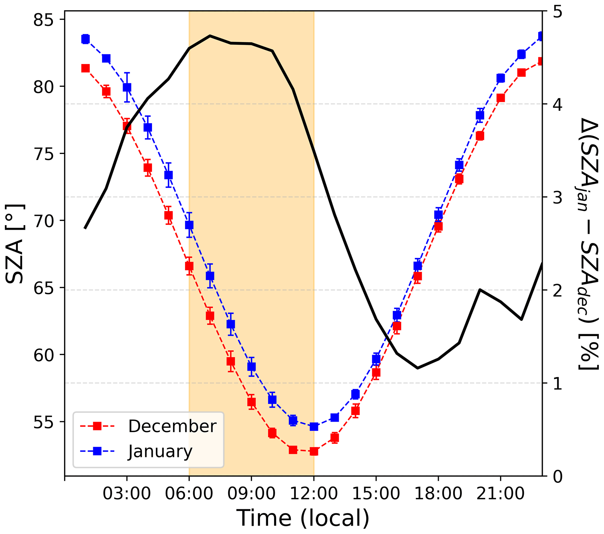
Figure 12 The left-hand scale shows the 2 h running ±1σ (error bars) of the period-averaged diurnal cycles of SZA (solar zenith angle) for both periods (December and January). The yellow-shaded area corresponds to the period where the NO₂:NO ratio is deviating from the steady-state equilibrium in December. The right-hand scale shows the percentage difference between SZA in January and in December, normalized to the December value.

A rapid parameterization of the dependence of the NO_x production, $P_{{\mathrm{NO}}_x}$ (pptv h⁻¹), to the position of the sun, SZA (^∘), has been established. For the calculation, a normalization over the SZA in December has been made. Additionally, in Fig. 7 it appears that the NO_x production is happening during daytime, with a SZA >70^∘; therefore, only the daily values (06:00 to 18:00 LT) were taken into account for this parameterization. Figure 13 shows the results of linear regressions for both periods, suggesting that it is possible to decipher the parameters linking the NO_x production to the SZA. Indeed, satisfactory R² values (0.984 for December and 0.727 for January) were found. Of course, this result is only an approach, and a thorough study of the NO_x production dependence on the sun's position would allow for the improvement of existing models and would reduce the uncertainties concerning the Antarctic nitrogen budget.

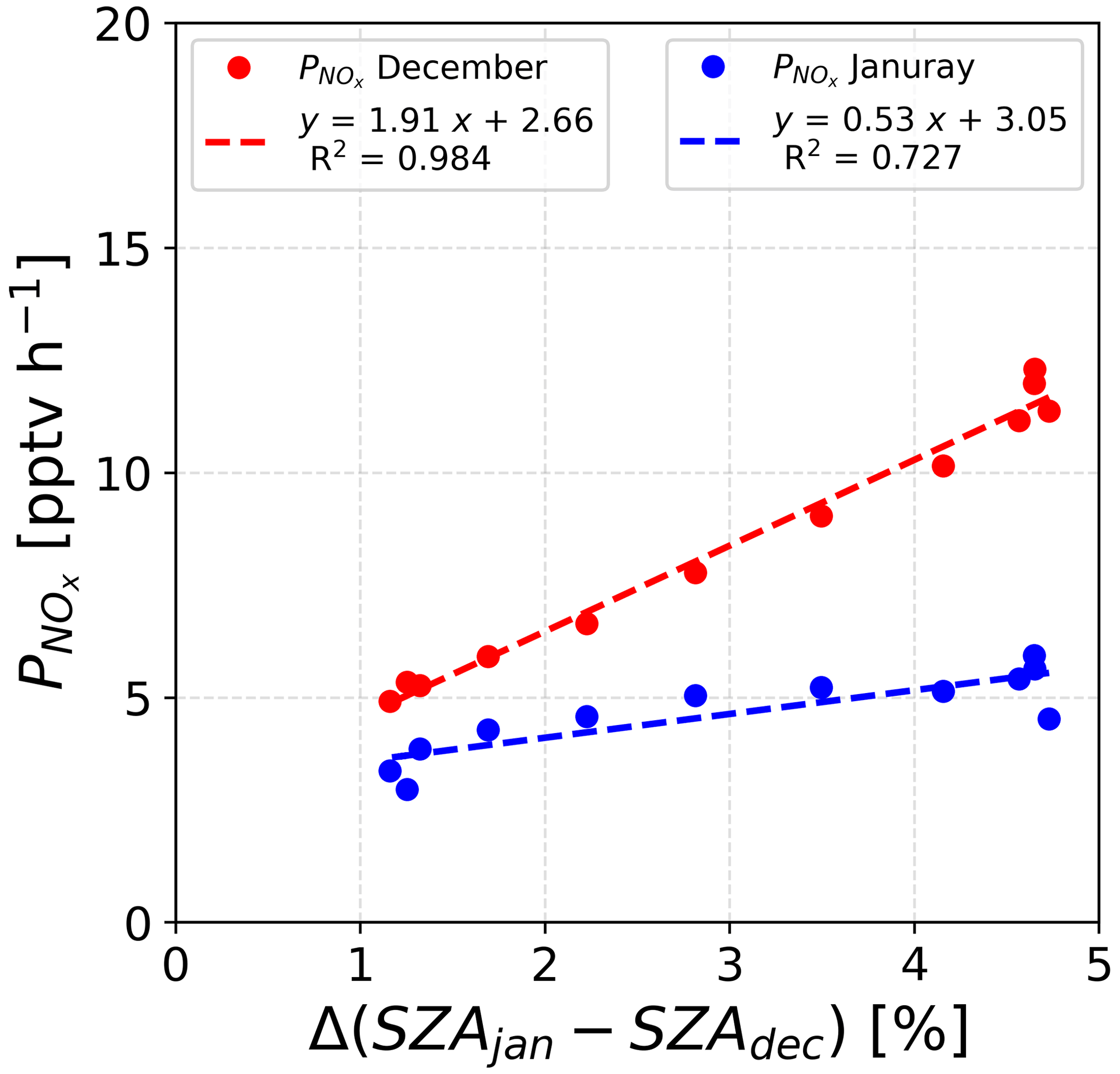
Figure 13 Correlations between the NO_x production and the Δ(SZA_jan−SZA_dec) normalized to the December value for both periods of atmospheric observations.

6 Conclusions

For the first time, direct and in situ atmospheric measurements of NO₂ were carried out in the Antarctic Plateau at Dome C. The summer variability of the NO₂:NO ratio was studied in light of this new set of observations. While the overall NO₂:NO ratio can be explained by the extended Leighton's relationship in certain periods, a high NO₂:NO ratio was estimated in the morning during the early photolysis season, which deviates from steady-state equilibrium and is not explained by the extended Leighton's relationship. The results of this study disagree with previous studies that found a systematic deviation from equilibrium, requiring around 50 pptv of halogenated radicals to explain such a NO₂:NO ratio. However, the required levels of halogenated species were never observed at Dome C. While differences in atmospheric dynamics and snow cover during the different campaigns could explain the discrepancies with previous studies, it may also be due to different detection techniques being used. In our study, NO₂ was measured directly for the first time at Dome C. The NO_x snow source was studied in the light of new results presented in Barbero et al. (2021), where a nitrate daily average photolysis rate constant, $J_{{\mathrm{NO}}_{\mathrm{3}}^{-}}$ = (2.37 ± 0.35) × 10⁻⁸ s⁻¹, for all different snow samples (at the depth and location of the Antarctic Plateau) taken from 10 December to 7 January is estimated. NO_x fluxes (expressed in molec. cm⁻² s⁻¹) from the snow surface source were estimated and converted into a production rate (in molec. cm⁻³ h⁻¹) using the polar boundary layer height (cm). A mean ratio of 1.92 ± 0.33 in the NO_x production between December and January was estimated in the early morning, with a factor of up to 2.6 difference in the surface snow NO_x production between December and January, corresponding to the deviation from photochemical equilibrium observed. Therefore, evaluation of the meteorological conditions and estimation of the NO_x snow source tend to identify the NO_x snow source and the position of the sun, through SZA measurement, as the main actors of the atmospheric oxidative capacity in the austral summer at Dome C. From our calculations, it appears that a 5 % difference in the SZA in the morning could lead to an excess of up to 5 times the NO₂:NO ratio when at steady state. Such a high sensitivity of the NO₂:NO ratio to the sun position is of importance to the atmospheric chemistry models, where such a parameter can be better adjusted in the future. However, even though the NO_x snow source might explain the differences between December and January in the NO_x cycle, this does not match the observed O₃ variations. In addition, even though the depletion of the NO_x reservoir throughout the light season might explain the lower levels of O₃ toward the end of the photolytic season, additional investigations into possible unidentified mechanisms or unidentified sinks of O₃ are needed to understand the O₃ consumption. The link between the stratospheric ozone hole inducing an enhancement in the incident UV radiation, and in turn causing an increase in the ice-to-atmosphere iodine emissions, has been stated by Spolaor et al. (2021). Therefore, in the future, additional field campaigns targeting halogenated radical measurements in snow and the troposphere in Antarctica are needed to allow the scientific community to fully understand the mechanisms driving the oxidative capacity of the polar atmosphere.

Appendix A: NOAA HYSPLIT backward trajectories reconstruction for the observation periods (Dome C is represented by the black star)

Using the HYSPLIT model (meteorological data taken from the archive GDAS1, i.e. 1^∘, global, 2006–present), 5 d (120 h) backward trajectories were conducted to characterize air masses arriving at Concordia. For each day of observation, four runs were computed at different times (UTC), 00:00, 06:00, 12:00 and 18:00 UTC, corresponding to 08:00, 14:00, 20:00 and 02:00 LT (day+1). Three atmospheric levels were considered above Concordia as a starting point to compute the back trajectories: 3200, 3400, and 3800 m a.m.s.l.​​​​​​​ (above mean sea level; i.e. at the snow surface and 200 and 400 m above Concordia, respectively).

A1 December

As mentioned in Sect. 2.1 of the main text, the meteorological conditions and air mass origins in December were favourable for atmospheric measurements for the purposes of our study. Indeed, one can see in Fig. A1 that the air masses were originating from the plateau during the observation period. On 9 December at 14:00 LT, i.e. 06:00 UTC, air masses at 3800 m a.m.s.l. were simulated to be originating from the Antarctic Peninsula, but this had no impact on our observations as we stopped them around 10:00 LT.

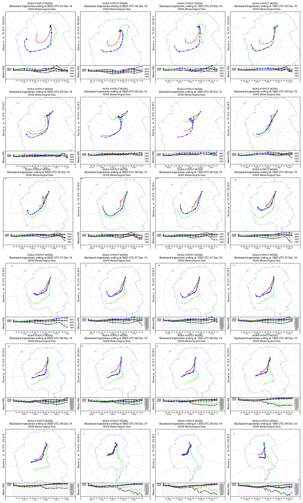
Figure A1 HYSPLIT 5 d backward trajectories from 4 to 9 December 2019. The model was run every 6 h for each day and at three different altitudes: 3800 (green), 3400 (blue), and 3200 m a.m.s.l. (red).

A2 January

As mentioned in Sect. 2.1 of the main text, the meteorological conditions and air mass origins in January were favourable for atmospheric measurements from 17 to 20 January (Fig. A2). However, the 10 ppbv drop in O₃ observed at the end of the observation period is suspected to be caused by oceanic inputs, as suggested by Legrand et al. (2009). On Fig. A3, a drastic change in the origin of the air masses is observed on 23 January between 06:00 (UTC) and 12:00 (UTC) or 14:00 and 20:00 LT, corresponding to the sudden drop in O₃ mixing ratio around 17:00–18:00 LT.

Figure A4 shows the HYSPLIT 10 d back trajectory estimation for 23 January ending at 20:00 LT at Dome C. One can see that the model predicts that the air masses are coming from the east coast of Antarctica in the 3400 m a.m.s.l. data, strengthening our conclusions of an air mass influenced by the ocean reaching the Antarctic Plateau and leading to the 10 ppbv O₃ drop observed in the early evening of 23 January 2020. Indeed, Legrand et al. (2009) showed that the origin of the air masses reaching Concordia influences the ozone level. The lowest values are observed when the air masses have spent at least 1 d over the ocean during the 5 d preceding their arrival at Concordia, and the highest values are found when the air masses have always travelled over the highest part of the Antarctic plateau.

Figure A2 HYSPLIT 5 d backward trajectories from 16 to 21 January 2020. The model was run every 6 h for each day and at three different altitudes: 3800 (green), 3400 (blue), and 3200 m a.m.s.l. (red).

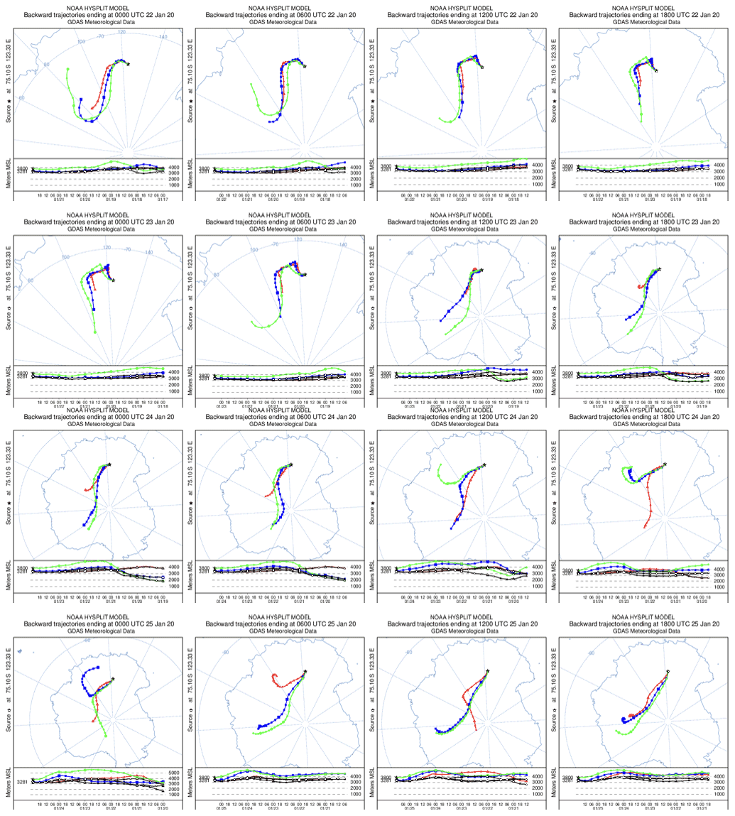
Figure A3 HYSPLIT 5 d backward trajectories from 22 to 25 January 2020. The model was run every 6 h for each day and at three different altitudes: 3800 (green), 3400 (blue), and 3200 m a.m.s.l. (red).

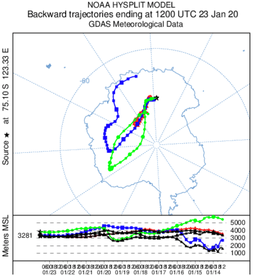
Figure A4 HYSPLIT 10 d backward trajectories of 23 January ending at 12:00 UTC (20:00 LT) at three different altitudes: 3800 (green), 3400 (blue), and 3200 m a.m.s.l. (red).​​​​​​​

Appendix B: Meteorological conditions during two periods of observations

The wind rose of the January period (Fig. B1d) shows strong wind from the west–north-west direction. Looking at Fig. B1c, a sudden change in the wind direction occurred in late January (around 23 January), strengthening our hypothesis that there were ocean air masses that might have reached Dome C at the end of January, explaining the 10 ppbv O₃ drop.

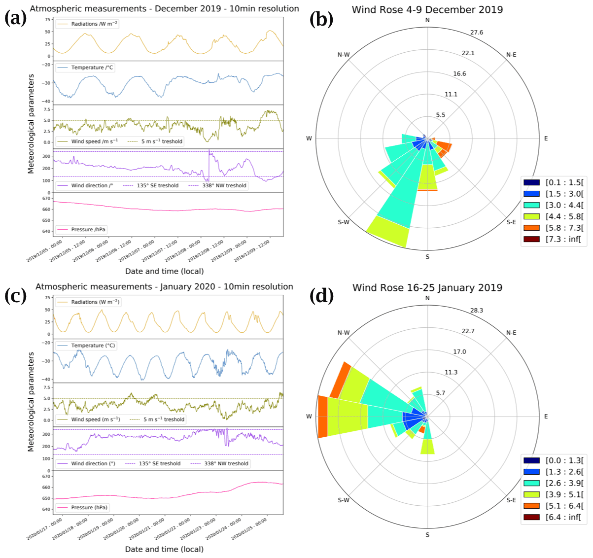
Figure B1 Panels (a) and (c) show local meteorological conditions (2 m observations) encountered during the periods of atmospheric observations measured by the local automatic weather station (Vaisala Milos 520) completed with a broadband UV radiometer in the spectral range 305–385 nm. Panels (b) and (d) show the corresponding wind rose (in m s⁻¹) at Dome C.

Appendix C: Snow tower experiment

Figure C1 shows the schematic of the snow tower device, along with a photograph of one of the snow towers. We can see the two partially buried snow towers at the ends of the diagram, as well as the fully exposed atmospheric mast in the middle.

Figure C1 Snow tower installation at Dome C.​​​​​​​

Appendix D: NO₂ and O¹D photolysis rate constant reconstruction: $J_{{\mathrm{NO}}_{\text{2-recons}}}$ and $J_{{\mathrm{O}}^{\mathrm{1}}{\mathrm{D}}_{\text{-recons}}}$

The $J_{{\mathrm{NO}}_{\text{2-recons}}}$ (in s⁻¹) is reconstructed using a correlation fit analysis between the UV radiations signal and the sparse $J_{{\mathrm{NO}}_{\mathrm{2}}}$ measurements obtained with the MetCon 2π spectral radiometer (Fig. D1). A 2^∘ polynomial function, Eq. (D1), was found to be the best correlation fit (dashed black line in Fig. D1).

$$\begin{array}{}\text{(D1)}& J_{{\mathrm{NO}}_{\text{2-recons}}}=a\times \mathrm{UV}+b\times {\mathrm{UV}}^{\mathrm{2}},\end{array}$$

where $J_{{\mathrm{NO}}_{\text{2-recons}}}$ is the reconstructed photolysis rate coefficient, a and b are the regression fit parameters using the Powell minimization method (Powell, 1964), and UV is the measured UV radiation.

Figure D1 Fit analysis for the reconstruction of the $J_{{\mathrm{NO}}_{\mathrm{2}}}$ signal.

Table D1 gives the values of a and b parameters for the photolysis rate constant at both periods.

Table D1 Polynomial regression fit parameters from Eq. (D1) applied to reconstruct the photolysis rate coefficient signal.

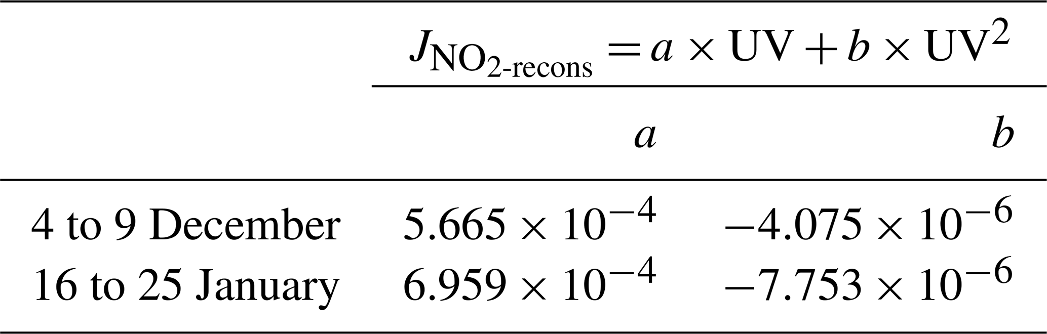
Figure D2 represents the comparison between the reconstructed signal and the actual observations. In the bottom panel, the residual $\mathrm{\Delta }{J}_{{\mathrm{NO}}_{\text{2-recons}}}$ is represented, showing a good agreement between the reconstructed signal and the original observations.

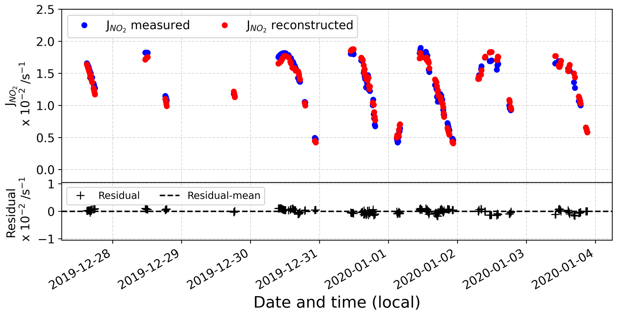
Figure D2 (top) Comparison between reconstructed and measured signal and (bottom) residual data.

The $J_{{\mathrm{O}}^{\mathrm{1}}{\mathrm{D}}_{\text{-recons}}}$ (in s⁻¹) is reconstructed using a correlation fit analysis between the UV radiation signal and the sparse $J_{{\mathrm{O}}^{\mathrm{1}}\mathrm{D}}$ measurements obtained with the MetCon 2π spectral radiometer (Fig. D3). A 2^∘ polynomial function, Eq. (D2), was found to be the best correlation fit (dashed black line in Fig. D3).

$$\begin{array}{}\text{(D2)}& J_{{\mathrm{O}}^{\mathrm{1}}{\mathrm{D}}_{\text{-recons}}}=c\times \mathrm{UV}+d\times {\mathrm{UV}}^{\mathrm{2}},\end{array}$$

where $J_{{\mathrm{O}}^{\mathrm{1}}{\mathrm{D}}_{\text{-recons}}}$ is the reconstructed photolysis rate coefficient, c and d are the regression fit parameters using the Powell minimization method (Powell, 1964), and UV is the measured UV radiation.

Figure D3 Fit analysis for the reconstruction of the $J_{{\mathrm{O}}^{\mathrm{1}}{\mathrm{D}}_{\text{-recons}}}$ signal.

Table D2 gives the values of c and d parameters for the photolysis rate constant at both periods.

Table D2 Polynomial regression fit parameters from Eq. (D2) applied to reconstruct the photolysis rate coefficient signal.

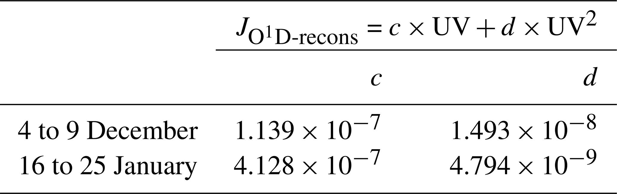
Figure D4 represents the comparison between the reconstructed signal and the actual observations. In the bottom panel, the residual $\mathrm{\Delta }{J}_{{\mathrm{O}}^{\mathrm{1}}{\mathrm{D}}_{\text{-recons}}}$ is represented, showing a good agreement between the reconstructed signal and the original observations.

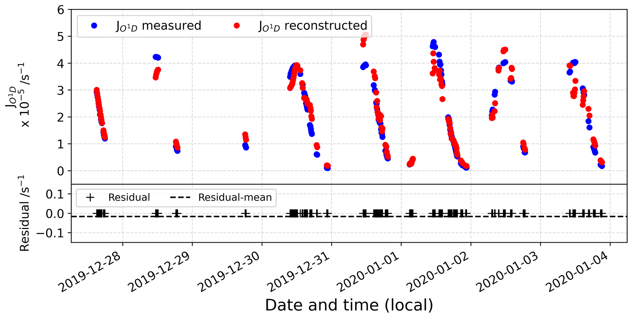
Figure D4 (top) Comparison between reconstructed and measured signal and (bottom) the residual data.

Appendix E: RO_x estimation from $J_{{\mathrm{NO}}_{\mathrm{2}}}$

Using the linear correlation between RO₂ and $J_{{\mathrm{NO}}_{\mathrm{2}}}$ given by Kukui et al. (2014) (Fig. E1a), the RO₂ data from OPALE campaign (Kukui et al., 2014), and the reconstructed $J_{{\mathrm{NO}}_{\mathrm{2}}}$ signal, we were able to estimate the RO₂ and HO₂ total number of molecules in the atmospheric boundary layer at Dome C during our periods of observation (Fig. E1b and c).

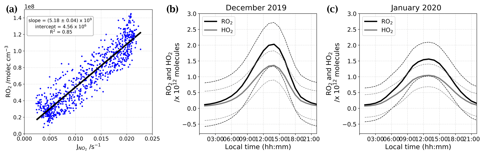
Figure E1 (a) Linear correlation between RO₂ and $J_{{\mathrm{NO}}_{\mathrm{2}}}$ taken from Kukui et al. (2014). Panels (b) and (c) show the total number of molecules of RO₂ (black) and HO₂ (grey) estimated for both periods of observation residuals.

Appendix F: Polar boundary layer height H_PBL

The regional climate model MAR, which has been applied extensively for studying the polar regions (e.g. Agosta et al., 2019; Gallée et al., 2015b; Gallée and Gorodetskaya, 2010) was used in its latest Antarctic configuration, i.e. version 3.11 (Kittel et al., 2021), including drifting-snow physics (Amory et al., 2021) at 35 km resolution, and forced by ERA5 reanalysis (https://www.ecmwf.int/en/forecasts, last access: 25 March 2021) to generate the boundary layer height extracted every hour to match the timestamp of our observations. Boundary layer heights at Dome C during both periods of observations extracted from the regional model MAR are presented in Fig. F1.

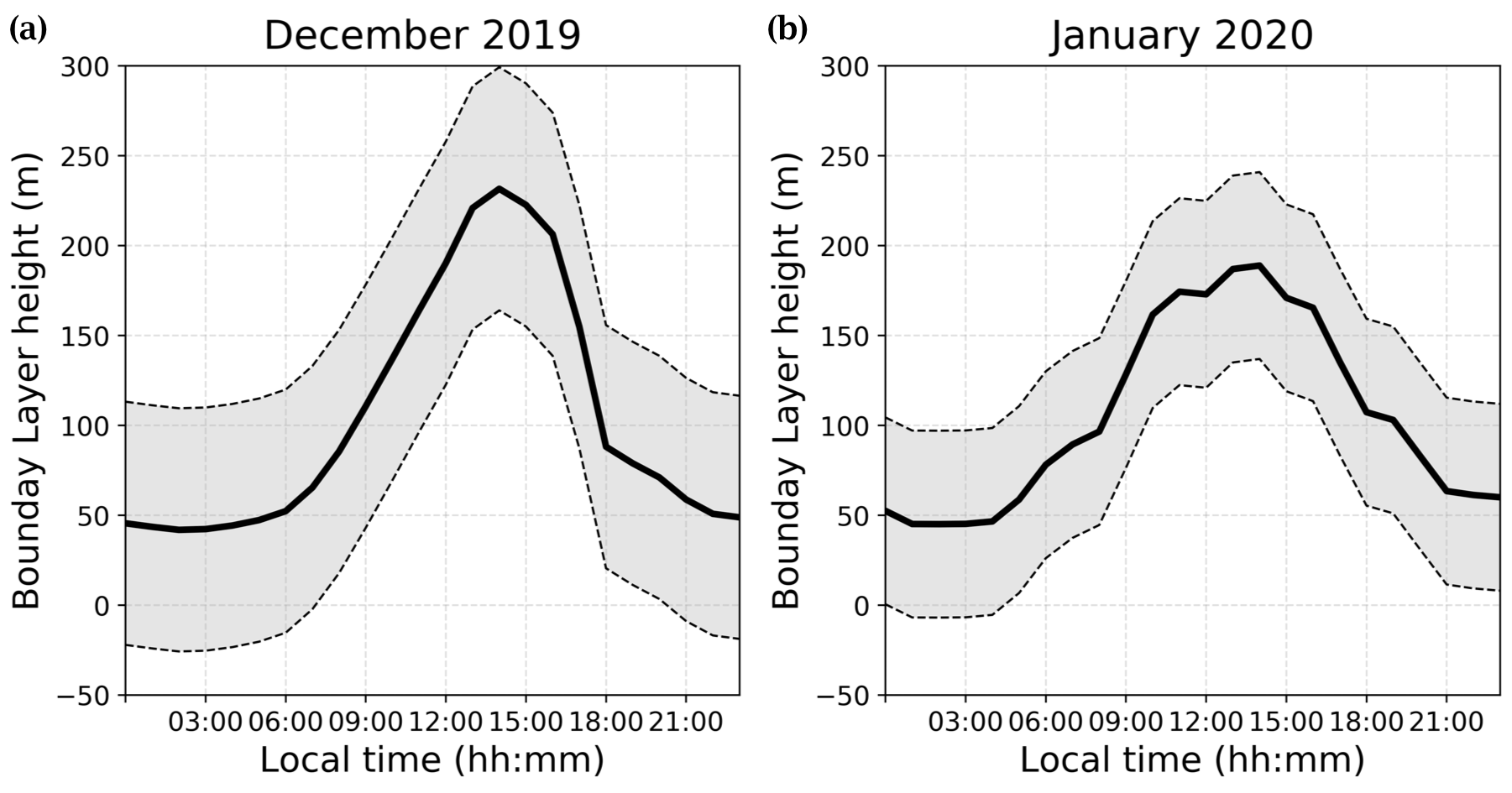
Figure F1 Atmospheric boundary layer height (PBL) (solid lines) and ±1σ (dashed lines) estimated for both periods by the MAR regional model.

Appendix G: Reactions and their chemical rates

The list of reactions at stakes in the Dome C troposphere with the associated daily average chemical rates based on their expression given by Atkinson (1998, 2003), $J_{{\mathrm{NO}}_{\mathrm{2}}}$ measurements from Atkinson et al. (2004, 2007), and $J_{{\mathrm{NO}}_{\mathrm{3}}^{-}}$ estimations from Barbero et al. (2021) for Dome C conditions.

• O_x reaction:

  $$\begin{array}{}\text{(GR1)}& {\mathrm{O}}_{\mathrm{3}}+h\mathit{\nu }\to \text{products}(J_{{\mathrm{O}}^{\mathrm{1}}\mathrm{D}}\approx \mathrm{3.76}\times {\mathrm{10}}^{-\mathrm{5}}{\mathrm{s}}^{-\mathrm{1}}).\end{array}$$

• HO_x reaction:

  $$\begin{array}{}\text{(GR2)}& \begin{array}{rl}{\mathrm{HO}}_{\mathrm{2}}& +{\mathrm{O}}_{\mathrm{3}}\to \mathrm{OH}+\mathrm{2}{\mathrm{O}}_{\mathrm{2}}\\ & (k_{{\mathrm{HO}}_{\mathrm{2}}+{\mathrm{O}}_{\mathrm{3}}}\approx \mathrm{1.2}\times {\mathrm{10}}^{-\mathrm{15}}{\mathrm{cm}}^{\mathrm{3}}\mathrm{molec}{.}^{-\mathrm{1}}{\mathrm{s}}^{-\mathrm{1}}).\end{array}\end{array}$$

• NO_x reaction:

  $$\begin{array}{}\text{(GR3)}& {\displaystyle }\begin{array}{rl}\mathrm{OH}& +\mathrm{NO}+M\to \mathrm{HONO}+M\\ & (k_{\mathrm{OH}+\mathrm{NO}}\approx \mathrm{1.0}\times {\mathrm{10}}^{-\mathrm{11}}{\mathrm{cm}}^{\mathrm{3}}\mathrm{molec}{.}^{-\mathrm{1}}{\mathrm{s}}^{-\mathrm{1}}),\end{array}\text{(GR4)}& {\displaystyle }\begin{array}{rl}\mathrm{OH}& +{\mathrm{NO}}_{\mathrm{2}}+M\to {\mathrm{HONO}}_{\mathrm{2}}+M\\ & (k_{\mathrm{OH}+{\mathrm{NO}}_{\mathrm{2}}}\approx \mathrm{1.8}\times {\mathrm{10}}^{-\mathrm{11}}{\mathrm{cm}}^{\mathrm{3}}\mathrm{molec}{.}^{-\mathrm{1}}{\mathrm{s}}^{-\mathrm{1}}),\end{array}\text{(GR5)}& {\displaystyle }\begin{array}{rl}{\mathrm{HO}}_{\mathrm{2}}& +\mathrm{NO}\to \mathrm{OH}+{\mathrm{NO}}_{\mathrm{2}}\\ & (k_{{\mathrm{HO}}_{\mathrm{2}}+\mathrm{NO}}\approx \mathrm{1.1}\times {\mathrm{10}}^{-\mathrm{11}}{\mathrm{cm}}^{\mathrm{3}}\mathrm{molec}{.}^{-\mathrm{1}}{\mathrm{s}}^{-\mathrm{1}}),\end{array}\text{(GR6)}& {\displaystyle }\begin{array}{rl}\mathrm{NO}& +{\mathrm{O}}_{\mathrm{3}}\to {\mathrm{NO}}_{\mathrm{2}}+{\mathrm{O}}_{\mathrm{2}}\\ & (k_{\mathrm{NO}+{\mathrm{O}}_{\mathrm{3}}}\approx \mathrm{6.3}\times {\mathrm{10}}^{-\mathrm{15}}{\mathrm{cm}}^{\mathrm{3}}\mathrm{molec}{.}^{-\mathrm{1}}{\mathrm{s}}^{-\mathrm{1}}),\end{array}\text{(GR7)}& {\displaystyle }\begin{array}{rl}\mathrm{HONO}& +h\mathit{\nu }\to \text{products}\\ & (J_{\mathrm{HONO}}\approx \mathrm{1.2}\times {\mathrm{10}}^{-\mathrm{3}}{\mathrm{s}}^{-\mathrm{1}}),\end{array}\text{(GR8)}& {\displaystyle }\begin{array}{rl}{\mathrm{NO}}_{\mathrm{2}}& +h\mathit{\nu }\to \text{products}\\ & (J_{{\mathrm{NO}}_{\mathrm{2}}}\approx \mathrm{1.3}\times {\mathrm{10}}^{-\mathrm{2}}{\mathrm{s}}^{-\mathrm{1}}).\end{array}\end{array}$$

• ClO_x reaction:

  $$\begin{array}{}\text{(GR9)}& {\displaystyle }\begin{array}{rl}\mathrm{ClO}& +\mathrm{NO}\to \mathrm{Cl}+{\mathrm{NO}}_{\mathrm{2}}\\ & (k_{\mathrm{ClO}+\mathrm{NO}}\approx \mathrm{2.1}\times {\mathrm{10}}^{-\mathrm{11}}{\mathrm{cm}}^{\mathrm{3}}\mathrm{molec}{.}^{-\mathrm{1}}{\mathrm{s}}^{-\mathrm{1}}),\end{array}\text{(GR10)}& {\displaystyle }\begin{array}{rl}\mathrm{ClO}& +{\mathrm{NO}}_{\mathrm{2}}+M\to {\mathrm{ClONO}}_{\mathrm{2}}+M\\ & (k_{\mathrm{ClO}+{\mathrm{NO}}_{\mathrm{2}}}\approx \mathrm{2.0}\times {\mathrm{10}}^{-\mathrm{11}}{\mathrm{cm}}^{\mathrm{3}}\mathrm{molec}{.}^{-\mathrm{1}}{\mathrm{s}}^{-\mathrm{1}}).\end{array}\end{array}$$

• BrO_x reaction:

  $$\begin{array}{}\text{(GR11)}& {\displaystyle }\begin{array}{rl}\mathrm{BrO}& +\mathrm{NO}\to \mathrm{Br}+{\mathrm{NO}}_{\mathrm{2}}\\ & (k_{\mathrm{BrO}+\mathrm{NO}}\approx \mathrm{2.5}\times {\mathrm{10}}^{-\mathrm{11}}{\mathrm{cm}}^{\mathrm{3}}\mathrm{molec}{.}^{-\mathrm{1}}{\mathrm{s}}^{-\mathrm{1}}),\end{array}\text{(GR12)}& {\displaystyle }\begin{array}{rl}\mathrm{BrO}& +{\mathrm{NO}}_{\mathrm{2}}+M\to {\mathrm{BrONO}}_{\mathrm{2}}+M\\ & (k_{\mathrm{BrO}+{\mathrm{NO}}_{\mathrm{2}}}\approx \mathrm{1.9}\times {\mathrm{10}}^{-\mathrm{11}}{\mathrm{cm}}^{\mathrm{3}}\mathrm{molec}{.}^{-\mathrm{1}}{\mathrm{s}}^{-\mathrm{1}}).\end{array}\end{array}$$

• IO_x reaction:

  $$\begin{array}{}\text{(GR13)}& {\displaystyle }\begin{array}{rl}\mathrm{IO}& +\mathrm{NO}\to \mathrm{I}+{\mathrm{NO}}_{\mathrm{2}}\\ & (k_{\mathrm{IO}+\mathrm{NO}}\approx \mathrm{2.8}\times {\mathrm{10}}^{-\mathrm{11}}{\mathrm{cm}}^{\mathrm{3}}\mathrm{molec}{.}^{-\mathrm{1}}{\mathrm{s}}^{-\mathrm{1}}),\end{array}\text{(GR14)}& {\displaystyle }\begin{array}{rl}\mathrm{IO}& +{\mathrm{NO}}_{\mathrm{2}}+M\to {\mathrm{IONO}}_{\mathrm{2}}+M\\ & (k_{\mathrm{IO}+{\mathrm{NO}}_{\mathrm{2}}}\approx \mathrm{1.2}\times {\mathrm{10}}^{-\mathrm{11}}{\mathrm{cm}}^{\mathrm{3}}\mathrm{molec}{.}^{-\mathrm{1}}{\mathrm{s}}^{-\mathrm{1}}).\end{array}\end{array}$$

  From the list above, one can see that the chemical sources of NO₂ and sinks from RO_x and XO have similar rates.