The impact of sulfur hexafluoride (SF₆) sinks on age of air climatologies and trends

Mean age of air (AoA) is a common diagnostic for the strength of the stratospheric overturning circulation in both climate models and observations. AoA climatologies and AoA trends over the recent decades of model simulations and proxies derived from observations of long-lived tracers do not agree. Satellite observations show much older air than climate models, and while most models compute a clear decrease in AoA over the last decades, a 30-year time series from measurements shows a statistically nonsignificant positive trend in the Northern Hemisphere extratropical middle stratosphere. Measurement-based AoA derivations are often founded on observations of the trace gas sulfur hexafluoride (SF₆), a fairly long-lived gas with a near-linear increase in emissions during recent decades. However, SF₆ has chemical sinks in the mesosphere that are not considered in most model studies. In this study, we explicitly compute the chemical SF₆ sinks based on chemical processes in the global chemistry climate model EMAC (ECHAM/MESSy Atmospheric Chemistry). We show that good agreement between stratospheric AoA in EMAC and MIPAS (Michelson Interferometer for Passive Atmospheric Sounding) is reached through the inclusion of chemical SF₆ sinks, as these sinks lead to a strong increase in the stratospheric AoA and, therefore, to a better agreement with MIPAS satellite observations. Remaining larger differences at high latitudes are addressed, and possible reasons for these differences are discussed. Subsequently, we demonstrate that the AoA trends are also strongly influenced by the chemical SF₆ sinks. Under consideration of the SF₆ sinks, the AoA trends over the recent decades reverse sign from negative to positive. We conduct sensitivity simulations which reveal that this sign reversal does not result from trends in the stratospheric circulation strength nor from changes in the strength of the SF₆ sinks. We illustrate that even a constant SF₆ destruction rate causes a positive trend in the derived AoA, as the amount of depleted SF₆ scales with increasing SF₆ abundance itself. In our simulations, this effect overcompensates for the impact of the accelerating stratospheric circulation which naturally decreases AoA. Although various sources of uncertainties cannot be quantified in detail in this study, our results suggest that the inclusion of SF₆ depletion in models has the potential to reconcile the AoA trends of models and observations. We conclude the study with a first approach towards a correction to account for SF₆ loss and deduce that a linear correction might be applicable to values of AoA of up to 4 years.

1 Introduction

The Brewer–Dobson circulation (BDC) describes the stratospheric transport circulation, consisting of the mean overturning circulation of air ascending in the tropical pipe, moving poleward and descending in the extratropics (Brewer, 1949; Dobson and Massey, 1956), as well as isentropic mixing. A good measure to diagnose this transport circulation is the age of stratospheric air (AoA), which is defined as the mean transport time of an air parcel from its entry into the stratosphere (or from the surface) to any point therein (Hall and Plumb, 1994; Waugh and Hall, 2002). In general circulation models (GCMs), AoA is commonly represented by an inert tracer with a strictly linear temporally increasing surface mixing ratio and is calculated as the corresponding time lag between the local mixing ratio and the mixing ratio at a reference point (Hall and Plumb, 1994). The same method can be applied to real long-lived tracers with a linear trend in tropospheric concentration, and AoA has been derived, for example, from balloon-borne in situ measurements of sulfur hexafluoride (SF₆) (Andrews et al., 2001; Engel et al., 2009, 2017). This trace gas is particularly suitable for these studies, as it is stable in the troposphere and stratosphere and its tropospheric concentrations have increased nearly linearly over recent decades. Along with observations of other trace gases, these measurements form a long-term dataset of observationally based AoA restricted to the Northern Hemisphere midlatitudes that covers more than 40 years. A near-global dataset of AoA covering 10 years from 2002 to 2012 was derived in Stiller et al. (2012), Haenel et al. (2015), and Stiller et al. (2017), who retrieved SF₆ distributions from MIPAS (Michelson Interferometer for Passive Atmospheric Sounding) satellite observations, but these cover a much shorter time period.

Observations and model simulations of AoA often disagree. AoA derived from observations is mainly older than simulated AoA (see, e.g., SPARC, 2010, and Dietmüller et al., 2018), and the AoA trend over recent decades even differs in sign between observations and models. While most climate models show a clear decrease in AoA over time (see, e.g., Butchart and Scaife, 2001, Garcia et al., 2011, and Eichinger et al., 2019), consistent with the simulated acceleration of the BDC in the course of climate change (see, e.g., Garcia and Randel, 2008), the time series of the observations presented in the studies by Engel et al. (2009), Ray et al. (2014), and Engel et al. (2017) show a (statistically nonsignificant) positive trend (note that Ray et al., 2014, also shows negative balloon AoA trends in the lower extratropical stratosphere). This discrepancy has been addressed in numerous studies. For example, Garcia et al. (2011) showed that, due to the concave growth rate of tropospheric SF₆ concentrations, the AoA trends derived from an SF₆ tracer are smaller than the trends derived from a synthetic, linearly growing AoA tracer (also after accounting for the nonlinear growth rates of SF₆). They noted that the sparse sampling of in situ observations can be the reason for the abovementioned trend discrepancies. Birner and Bönisch (2011) as well as Bönisch et al. (2011) argued that differences in the changes between the deep and the shallow BDC branch can possibly explain these. Ploeger et al. (2015) showed that the residual circulation transit time cannot explain the AoA trends and that the integrated effect of mixing (which is coupled to residual circulation changes; see Garny et al., 2014) is crucial. Moreover, Stiller et al. (2017) could explain a hemispheric asymmetry by a shift of subtropical transport barriers. In a study based on a chemistry transport model, Kouznetsov et al. (2020) showed that changes in SF₆-derived apparent AoA over 1 decade are highly influenced by the SF₆ sink and can even turn positive. However, a comprehensive understanding of the magnitude of the individual effects on the AoA trend depending on altitude and latitude is still missing.

SF₆ sinks lead to an older apparent AoA (see, e.g., Waugh and Hall, 2002, and Kouznetsov et al., 2020) as well as shorter lifetimes. Leedham Elvidge et al. (2018) evaluated AoA from several tracers including SF₆ and found clear differences between them, indicating a shorter SF₆ lifetime than previously assumed. The strongest chemical SF₆ removal reactions take place in the mesosphere; the most important removal processes are electron attachment and UV photolysis, but these processes have not yet been precisely quantified. Ravishankara et al. (1993) estimated an SF₆ lifetime of 3200 years, and Reddmann et al. (2001) found a lifetime of between 400 and 10000 years, depending on the assumed loss reactions and electron density. A more recent model study by Kovács et al. (2017), who used the Whole Atmosphere Community Climate Model (WACCM) to determine the atmospheric lifetime of SF₆, reported a mean SF₆ lifetime of 1278 years, and Ray et al. (2017) provided a range between 580 and 1400 years based on in situ measurements in the stratospheric polar vortex. The most recent model study of Kouznetsov et al. (2020), who performed simulations of tracer transport with a chemical transport model, shows an SF₆ lifetime ranging between 600 and 2900 years. Due to these uncertainties and the complex computation of the chemical reactions, most model studies do not consider any SF₆ sinks for the calculation of AoA from SF₆ mixing ratios. This can explain why most climate models generally show younger stratospheric air than observations, in particular within the polar vortices (e.g., Haenel et al., 2015; Ray et al., 2017).

In the present study, we apply the chemistry climate model EMAC (ECHAM MESSy Atmospheric Chemistry; Jöckel et al., 2010, 2016) with the aim of understanding the effects of SF₆ sinks on tracer-derived AoA and its long-term trends. Specifically, for the first time, we calculate the effect of the sinks on the long-term trend in SF₆-derived AoA and quantify how this effect is modulated by circulation changes (recent climate change), specified model dynamics, or by changes in the abundance of relevant species for SF₆ chemistry. Furthermore, we analyze the contribution of the SF₆ sinks themselves on the long-term trend in SF₆-based AoA. As an outlook, we thereupon provide first thoughts on how to apply an AoA correction to observations taking SF₆ sinks into account. The chemistry climate model uses the second version of the Modular Earth Submodel System (MESSy2) to link multi-institutional computer codes. In our simulations, we employed the MESSy submodel “SF6” which explicitly calculates SF₆ sinks based on physical processes (based on Reddmann et al., 2001), rather than on crude parameterizations. We apply a correction for the nonlinear growth of SF₆ in the calculation of AoA, based on Fritsch et al. (2020), which allows for the quantification of the effect of SF₆ sinks on SF₆-based AoA in isolation. In Sect. 2, we describe the EMAC model and the SF6 submodel as well as the observational data that we use for comparison. Section 3 contains a comparison of the EMAC climatologies with MIPAS data, a comparison of the EMAC trends with MIPAS and balloon-borne measurements, and an analysis of the results of two sensitivity simulations. The model results are discussed in the following using theoretical considerations of the effects of sinks on AoA trends (Sect. 4), including first thoughts on possible correction methods for the sinks, that are highly desirable for the use of observational data. In Sect. 5, we discuss the results and provide some concluding remarks.

2 Atmospheric model

2.1 EMAC model

For this study, we use the EMAC (ECHAM MESSy Atmospheric Chemistry, v2.54.0; Jöckel et al., 2010, 2016) model, a numerical chemistry and climate model (CCM) system. It contains the general circulation model (GCM) ECHAM5 (ECMWF Hamburg; Roeckner et al., 2003), with its spectral dynamical core, as well as the MESSy (Modular Earth Submodel System; Jöckel et al., 2005, 2010) submodel coupling interface. The latter is a modular interface structure for the standardized control of process-based modules (submodels) and their interconnections. We apply the model in a T42 horizontal (∼ 2.8^∘ × 2.8^∘) resolution with 90 layers in the vertical and explicitly resolved middle-atmosphere dynamics (T42L90MA). In this setup, the uppermost model layer is centered at 0.01 hPa, and the vertical resolution in the upper-troposphere–lower-stratosphere (UTLS) region is 500–600 m. In the standard reference setup, we use the basic EMAC modules for dynamics, radiation, clouds, and diagnostics (AEROPT, CLOUD, CLOUDOPT, CVTRANS, E5VDIFF, GWAVE, ORBIT, OROGW, PTRAC, QBO, RAD, SURFACE, TNUDGE, TROPOP, VAXTRA; the reader is referred to Jöckel et al., 2005, 2010, for details on these submodels). Additionally we included the new submodel SF6.

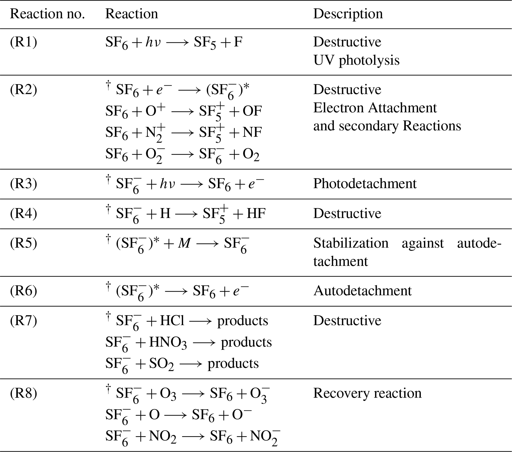
Table 1 Chemical reactions of SF₆. The labeling of the various reactions mirrors the style used by Reddmann et al. (2001). Reactions labeled with † are included in the SF6 submodel.

2.2 Submodel SF6

The submodel SF6 is used to calculate the lifetime of SF₆ by explicitly accounting for the sinks of SF₆ in the mesosphere. The submodel is operationally available for all users in MESSy from version 2.54.0 onward. The calculation method for this is based on the reaction scheme of Reddmann et al. (2001). The most important reaction involved in the chemical degradation of SF₆, namely electron attachment, is included in the SF₆ submodel. The configuration of the submodel allows for a simple exponential profile for the electron field and a more complex field based on Brasseur and Solomon (1986); in the present study, we use the latter option. It depends on altitude, latitude, solar zenith angle, air density, and day of year. In contrast to Reddmann et al. (2001), UV photolysis of SF₆ is not included in the submodel. The loss rate by photolysis is several orders of magnitude weaker than that of electron attachment up to altitudes of about 100 km (see, e.g., Fig. 9 in Totterdill et al., 2015) and is, therefore, not relevant for the focus of our study. Further reactions considered are the photodetachment of ${\mathrm{SF}}_{\mathrm{6}}^{-}$ (Datskos et al., 1995); the destruction of ${\mathrm{SF}}_{\mathrm{6}}^{-}$ by atomic hydrogen, hydrogen chloride, and ozone (Huey et al., 1995); the stabilization of excited ${\mathrm{SF}}_{\mathrm{6}}^{-}$ by collisions; and the autodetachment of ${\mathrm{SF}}_{\mathrm{6}}^{-}$. An overview is provided in Table 1. Reddmann et al. (2001) used climatological profiles for the aforementioned gases, whereas channel objects (see Jöckel et al., 2016) are used in our submodel. Such channel objects can be calculated in other submodules (e.g., interactive chemistry), prescribed as external time series (in this study), or just be simple climatologies. The autodetachment rate can be chosen in the namelist and was set to 10⁶ s⁻¹ (see Reddmann et al., 2001). For a general overview of the various reactions, see Fig. S1 in the Supplement.

(Jöckel et al., 2016)(Dee et al., 2011)(Jöckel et al., 2016)

Table 2 Overview of simulations undertaken in this study

GHGs refers to greenhouse gases, SSTs refers to sea surface temperatures, and SIC refers to sea ice concentration.

2.3 Simulation setup

The simulations performed in this study include a more comprehensive approach for the calculation of the SF₆ sinks. We use a climate chemistry model (as opposed to studies based on chemistry transport models as, e.g., in Kouznetsov et al., 2020) and use a more comprehensive SF6 submodel than previous chemistry climate model studies (see, e.g., Marsh et al., 2013, for WACCM). Other than the SF6 submodel, no interactive chemistry is activated in the simulations for this study. The reactant species involved in the SF₆ chemistry (HCl, H, N₂, O₂, O(³P), and O₃) and the radiatively active gases (CO₂, CH₄, N₂O, and O₃) are transiently prescribed from the ESCiMo RC1-base-07 simulation (see Jöckel et al., 2016) as monthly and zonal means. Moreover, we prescribe the Hadley Centre Sea Ice and Sea Surface Temperature (HadISST) dataset, the CCMI-1 volcanic aerosol dataset (for its effect on infrared radiative heating, see Arfeuille et al., 2013, and Morgenstern et al., 2017), and quasi-biennial oscillation (QBO) nudging (see Jöckel et al., 2016). To compute the photodetachment rate of ${\mathrm{SF}}_{\mathrm{6}}^{-}$, we follow Reddmann et al. (2001) and use the extraterrestrial solar photon flux with no attenuation of the UV-photon flux, as provided by WMO (1986). Our simulations range from 1950 to 2011; however, at least the first 10 years have to be considered as a spin-up period. The projection simulation runs from 1950 to 2100 with the SF₆ reactant species and greenhouse gases (GHGs) prescribed from the ESCiMo RC2-base-04 simulation (see Jöckel et al., 2016) as monthly and zonal means. In addition to the reference (REF) simulation, we performed two sensitivity simulations and one specified dynamics simulation. The two sensitivity simulations are as follows: the CSS (constant reaction partners for SF₆ sinks) sensitivity simulation differs from the REF simulation only with respect to the constant mixing ratios of the reactant species (see above) that influence the SF₆ sinks. For that purpose, we kept the mixing ratios at the level of the start of the simulation (year 1950 on repeat). With this simulation, we aim to address the influence of the reactant species involved in the SF₆ sink reactions. The second sensitivity simulation, referred to as TS2000, is not a transient simulation, as is the REF simulation, but is instead a time slice simulation with climate conditions (GHGs; sea surface temperatures, SSTs; and SICs) of the year 2000 (climatology of the 1995–2004 period). Furthermore, the reactant species for the SF₆ sinks have been averaged over the 1995–2004 period for the TS2000 simulation. This will allow us to investigate the effects of the SF₆ sinks under a constant climate. In the specified dynamics (SD) simulation, we apply Newtonian relaxation (“nudging”) towards ERA-Interim (Dee et al., 2011) reanalysis data of potential vorticity, divergence, temperature, and the logarithmic surface pressure up to 1 hPa. This assures that the meteorological situation largely resembles the ERA-Interim data. The flexible structure of MESSy allows us to use the same executable for all simulations, with the differences between them realized through changes in aforementioned namelist settings (see Jöckel et al., 2005). A summary of the simulations used in this study can be found in Table 2.

2.4 Satellite and in situ data

The MIPAS (Michelson Interferometer for Passive Atmospheric Sounding) instrument on Envisat (Environmental Satellite) allowed for the retrieval of SF₆ by measuring the thermal emission in the mid-infrared, while orbiting the Earth sun-synchronously 14 times a day. This high-resolution Fourier transform spectrometer measured at the atmospheric limb and provided data for SF₆ retrievals in full spectral resolution from 2002 to 2004 and in reduced resolution from 2005 to 2012 between 6 and 40 km of altitude (Stiller et al., 2012; Haenel et al., 2015). In this study, a newer version of the MIPAS dataset, existing as of 2019, will be shown (Stiller, 2021) in which new SF₆ absorption cross sections have been used for the SF₆ retrieval (Stiller et al., 2020; Harrison, 2020). Except for the newer absorption cross sections for SF₆ and the consideration of a trichlorofluoromethane (CFC-11) band in the vicinity of the SF₆ signature, the SF₆ retrieval and conversion into AoA was done according to the description by Haenel et al. (2015). In particular, the Level-1b data version is still V5.

Engel et al. (2009) collected available air samples of SF₆ and CO₂ from a balloon-borne cryogenic whole-air sampler flown during 27 balloon flights, with data up to 43 km, and reanalyzed these samples in a self-consistent manner. The derived SF₆ data cover the years from 1975 to 2005 (with a gap between 1985 and 1994) and the midlatitudes between 32 and 51^∘ N. As AoA profiles from midlatitudes above approximately 25 km or 30 hPa are constant over altitude, a mean midlatitude middle-stratospheric AoA value from each profile was determined by averaging the vertical profile between 30 hPa and the top balloon flight height. With this procedure, a time series of midlatitude middle-stratospheric AoA values could be determined back to 1975. It is important to note that part of the Engel et al. (2009) AoA time series is derived from CO₂ measurements. In this paper, only the AoA data points derived from SF₆ are used. Engel et al. (2017) extended the initial dataset from Engel et al. (2009) to 2016, but the AoA here is derived from CO₂ measurements and is, thus, also excluded.

2.5 Analysis method

The basic concepts for the calculation of mean AoA are introduced in Hall and Plumb (1994). In the case of a tracer with a linear increasing lower boundary condition, AoA can be determined by the time lag between the mixing ratio at a given point in the atmosphere and the same mixing ratio of the reference time series. As for any realistic tracer, SF₆ does not exhibit perfectly linear growth, for which adjustments in the AoA calculation are needed. This study follows the calculation method employed by studies such as Engel et al. (2009), which was introduced in Volk et al. (1997). The calculation uses a polynomial fit to the reference time series to approximate mean AoA. However, in our study, we modified the parameters compared with those used in Engel et al. (2009) to ensure that (passive) SF₆-based AoA agrees with the ideal AoA derived from the linear tracer, following Fritsch et al. (2020). Specifically, in our calculations, we used a ratio of moments of 1.0 years and a fraction of input of 95 %. Further, we used the SF₆ mixing ratio averaged over 20^∘ S–20^∘ N at the ground as the reference time series. Due to the availability of data, this reference region is also used in Engel et al. (2009) with balloon-borne observations.

Figure 1 Vertical SF₆ profiles for the four tracers from the SD simulation averaged over (a) 30–50^∘ N (zonally averaged) for 2007–2010 and (b) 60–80^∘ N, 0–100^∘ E for 5 March 2000. Horizontal lines show the SF₆ spread over the selected longitudes. Dark blue represents the nonlinear tracer with sinks tr(WS, SF₆), light blue represents the nonlinear tracer without sinks tr(NS, SF₆), light green represents the idealized tracer tr(NS, lin), and dark green represents the linear tracer with sinks tr(WS, lin). In panel (a), the SF₆ mixing ratios obtained from MIPAS (Stiller et al., 2020; Stiller et al., 2022) are shown in black. Black error bars depict the standard deviation of MIPAS SF₆, and pink error bars show the systematic error of MIPAS. The systematic error is comprised of errors in the spectroscopic data and uncertainty in the instrumental line shape, which results in a systematic error of 2 % for the lower stratosphere (10 km) and 11 % for the upper stratosphere (60 km). See Stiller et al. (2020) for details. Black crosses in panel (b) represent the balloon-borne measurements (Ray et al., 2017) taken on 5 March 2000 at Kiruna, Sweden (67^∘ N).

For the derivation of AoA from MIPAS SF₆ observations, Stiller et al. (2008, 2012) and Haenel et al. (2015) used a slightly smoothed version of the global mean of SF₆ surface measurements as the reference time series instead of SF₆ at the stratospheric entry point, which is not available from observations (see, e.g., Dlugokencky, 2005). The nonlinearity of the reference curve was considered by its convolution with an idealized age spectrum parameterized as a function of the mean age within an iterative approach. For more details, see Stiller et al. (2012) and Haenel et al. (2015).

In our simulations, the AoA calculations are applied to a total of four tracers, which can be organized into two groups. The first assumes a strict linear growth of SF₆, producing a linear reference curve, whereas the second considers a realistic growth of SF₆ based on observed emissions, creating a nonlinear SF₆ reference curve. Technically, in our simulations these “emissions” are realized via lower boundary conditions, which are based on surface observations, as in Jöckel et al. (2016). As previously mentioned, SF₆ undergoes chemical degradation predominantly in the mesosphere. Consequently, the absence or presence of mesospheric sinks is additionally considered, resulting in a total of four tracers: tr(WS, SF₆), tr(NS, SF₆), tr(WS, lin), and tr(NS, lin). The labeling of these depends on the chemistry involved (with sinks: “WS”; without (no) sinks: “NS”) and the growth assumed (linear: “lin”; nonlinear: “SF₆”) and follows the pattern tr(Chemistry, Growth). When referring to simulations with a specific tracer, the labeling will follow the notation Simulation(Chemistry, Growth), and similarly we use the following notation for AoA inferred from the tracer used in a simulation: AoA(Chemistry, Growth)_SIM. For example, AoA from the reference simulation based on the tracer with mesospheric sinks and nonlinear (SF₆-emission-based) increase is referred to as “AoA(WS, SF₆)_REF”, and AoA inferred from the linear tracer without mesospheric sinks in the reference simulation is denoted as “AoA(NS, lin)_REF”.

3 Results

3.1 SF₆ mixing ratios

In order to evaluate the SF₆ mixing ratios simulated by the EMAC model, we first analyze the four tracers in the SD simulation in comparison to observational data. This study does not perform a detailed comparison of SF₆ profiles, as the major aim is not an in-depth evaluation of the SF6 submodel but rather a quantification of the potential effects of the SF₆ sinks on AoA and its long-term trends. However, to ensure that SF₆ values in the EMAC model are within the range of observational estimates, we perform selected comparisons to data from Ray et al. (2017) and MIPAS SF₆ (Stiller et al., 2020, paper in preparation). Figure 1a depicts the modeled SF₆ vertical profile climatologies in comparison with MIPAS SF₆. Figure 1b shows the modeled SF₆ vertical profiles and balloon-borne measurements of SF₆ (Ray et al., 2017) on a particular day. The former comparison is for zonal mean SF₆ averaged over 30–50^∘ N and 2007–2010. These years have been chosen as the dataset is complete in this period. The error bars represent the standard deviation of the zonal mean ensemble, which consists of the measurement noise error of MIPAS, further random error sources from the retrieval (e.g., temperature uncertainties), the natural variability over the longitudes of the latitude band, and the 4 years of averaging (2007–2010).

Figure 1b shows modeled SF₆ mixing ratios of the day of the balloon flight. The balloon was launched on 5 March 2000 at 67^∘ N in Kiruna, Sweden. To ensure that the SF₆ profile is based on air masses from within the vortex, modeled SF₆ values are averaged over 65–80^∘ N and 0–100^∘ E, which corresponds to the area of the vortex core for the given day. The standard deviation of SF₆ for 0–100^∘ E averaged over the respective latitude range is shown as error bars.

The tracers with nonlinear growth in the SD simulation show smaller tropospheric SF₆ mixing ratios than the linear tracers (Fig. 1a, b). This can be explained by the two different growth scenarios of SF₆ and the prescribed lower boundary conditions (see Fig. S2 in the Supplement). The sinks do not have a considerable effect in the troposphere; hence, the effect of the SF₆ sinks only becomes noticeable higher up. Furthermore, the effect of the SF₆ depletion becomes increasingly evident with altitude. This is portrayed in the growing differences with altitude between tr(WS, lin) and tr(NS, lin) and the nonlinear equivalent. The differences particularly increase for the tracers with linear emissions, as these exhibit higher SF₆ mixing ratios and, hence, experience greater SF₆ depletion than those with nonlinear boundary conditions. Due to the small turnaround times for air in the middle atmosphere, the tracers without sinks exhibit a very low decrease in the SF₆ mixing ratios with altitude.

Figure 1a shows that the EMAC-simulated nonlinear SF₆ is within the observed range of MIPAS SF₆. Below 30 km, MIPAS SF₆ mixing ratios are smaller, with a near-constant offset of approximately 0.5 pmol mol⁻¹ up to 20 km. Above 30 km, MIPAS SF₆ shows larger mixing ratios than EMAC. This means that EMAC SF₆ (SD(WS, SF₆)) shows a larger decrease with altitude than MIPAS SF₆, suggesting that the sinks in EMAC are too strong. Another explanation could be overly strong vertical mixing in EMAC. However, the EMAC SF₆ lies within the MIPAS uncertainty range throughout the atmosphere. The standard deviation increase with height in MIPAS SF₆ can be attributed to the decrease in the SF₆ signal with height, which leads to an increase in the noise error of SF₆. Additionally, the natural variability in SF₆ itself, as well as the evolution of SF₆ over time, contribute to the increasing standard deviation in the MIPAS SF₆ profile. The increase in the standard deviation with height can also be seen in the EMAC SF₆ profiles, particularly in the tracers tr(WS, SF₆) and tr(WS, lin). However, it is (by far) not as large as in the MIPAS data because the simulations have no measurement error and possibly show a smaller natural variability than the observations.

The balloon flight SF₆ profile (Ray et al., 2014) in Fig. 1b largely resembles the profile of the realistically modeled tracer tr(WS, SF₆). Below 25 km, the modeled SF₆ profile shows a constant high bias of around 0.3 pmol mol⁻¹, presumably due to the lower boundary conditions used. Larger discrepancies can be seen between 25 and 35 km altitude, with higher mixing ratios of the modeled SF₆. As the data presented in Fig. 1b are only for a specific day and region, the particular meteorological situation and location of the balloon can be crucial for the comparison.

3.2 SF₆ lifetimes

The atmospheric lifetime of SF₆ can be used as an indicator for the accuracy of the SF₆ degradation scheme. We calculate the lifetime following Eq. (1) in Sect. 3 of Reddmann et al. (2001), namely

$$\begin{array}{}\text{(1)}& {\displaystyle \frac{\mathrm{d}\left[{\mathrm{SF}}_{\mathrm{6}}\right]}{\mathrm{d}t}}=-[k_{\mathrm{1}}+k_{\mathrm{2}}(\mathrm{1}-\mathit{ϵ}\mathit{\eta }\left)\right]\left[{\mathrm{SF}}_{\mathrm{6}}\right].\end{array}$$

It is based on the reaction rates (k_i) of the chemical reactions (R_i) marked in Table 1, the branching fraction ϵ (taken as 0.999; see Reddmann et al., 2001), and the efficiency of the SF₆-recovery reactions (η), where η is calculated as

$$\begin{array}{}\text{(2)}& \mathit{\eta }={\displaystyle \frac{k_{\mathrm{5}}(k_{\mathrm{3}}+k_{\mathrm{8}})+k_{\mathrm{6}}(k_{\mathrm{3}}+k_{\mathrm{4}}+k_{\mathrm{7}}+k_{\mathrm{8}})}{(k_{\mathrm{5}}+k_{\mathrm{6}})(k_{\mathrm{3}}+k_{\mathrm{4}}+k_{\mathrm{7}}+k_{\mathrm{8}})}}.\end{array}$$

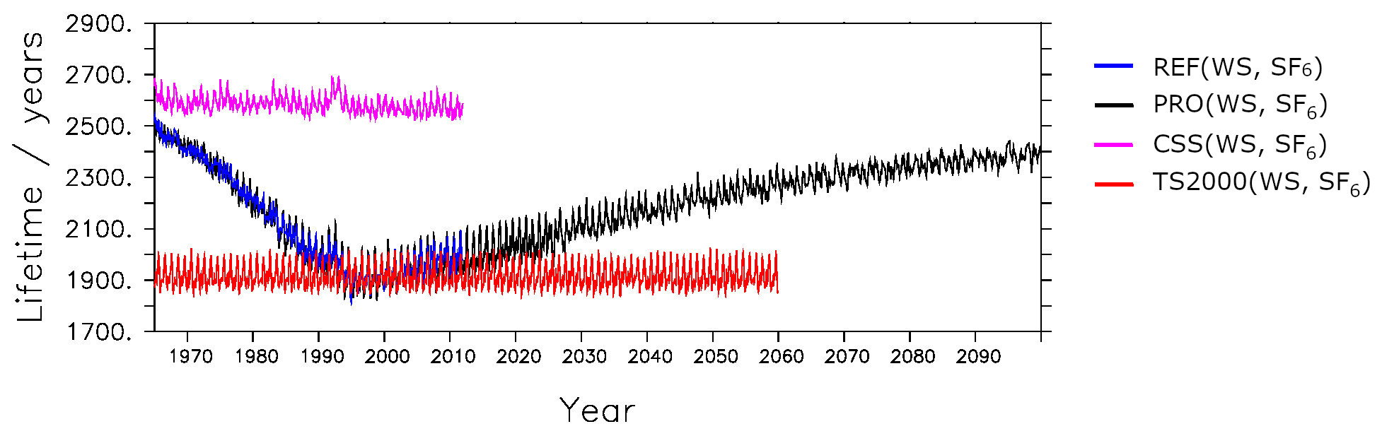
Figure 2 Global stratospheric and mesospheric lifetimes of SF₆ calculated from the tracer with realistic lower boundary conditions and SF₆ sinks (tr(WS, SF₆)). Blue represents the reference simulation (REF), black represents the projection simulation (PRO), pink represents the constant reactant species simulation (CSS), and red represents the time slice 2000 simulation (TS2000).

Only the realistic tracer tr(WS, SF₆) is considered. The reference simulation yields an average lifetime of 2101 years. Reddmann et al. (2001) carried out sensitivity experiments with this scheme, using various options for the chemical mechanisms. In this way, the lifetime could be varied between 400 and 10 000 years. Our value is below the value of 3200 years calculated by Ravishankara et al. (1993) but above the values of 1278 and 850 years of the more recent studies by Kovács et al. (2017) and Ray et al. (2017), respectively. In another new modeling study, Kouznetsov et al. (2020) presented a range of 600–2900 years. Therefore, our value of around 2100 years is within, although rather at the upper range, of the uncertainties. In contrast to the comparison of the model results with SF₆ observations shown in the previous section, our lifetime value points towards rather weak SF₆ sinks in our scheme. To assess the variability in the atmospheric SF₆ lifetime, we show the time series of the SF₆ lifetimes for the four simulations that were described in Sect. 2 (Fig. 2). The lifetime of the REF simulation lies at about 2500 years in 1965 and decreases by approximately 25 % to 1900 years in 2011. The lifetime of the projection simulation behaves similarly and increases to about 2400 years by the year 2100. This shape of the lifetime resembles that of projected O₃ (see, e.g., Eyring et al., 2007), which is reflected in the ESCiMo simulations (Jöckel et al., 2016) from which the O₃ and the other SF₆ reactant species are prescribed here. However, our SF₆ degradation scheme includes a number of simplifications, which can modify the lifetimes. For example, a constant profile is used to prescribe the sinks through NO. This can simplify the long-term variability in the SF₆ lifetimes by making it overly dependent on the species that are transiently prescribed in the simulations. Apart from seasonal variations, the lifetimes of the CSS and the TS2000 simulations are fairly constant, their lifetime values lie around 2600 and 1900 years, respectively. The fact that the lifetimes of the CSS simulations are fairly constant implies that the long-term trends of the SF₆ lifetimes can mostly be attributed to the abundance of the species involved in the SF₆ degradation. Variations in stratospheric temperatures or the circulation strength seem to only play a minor role.

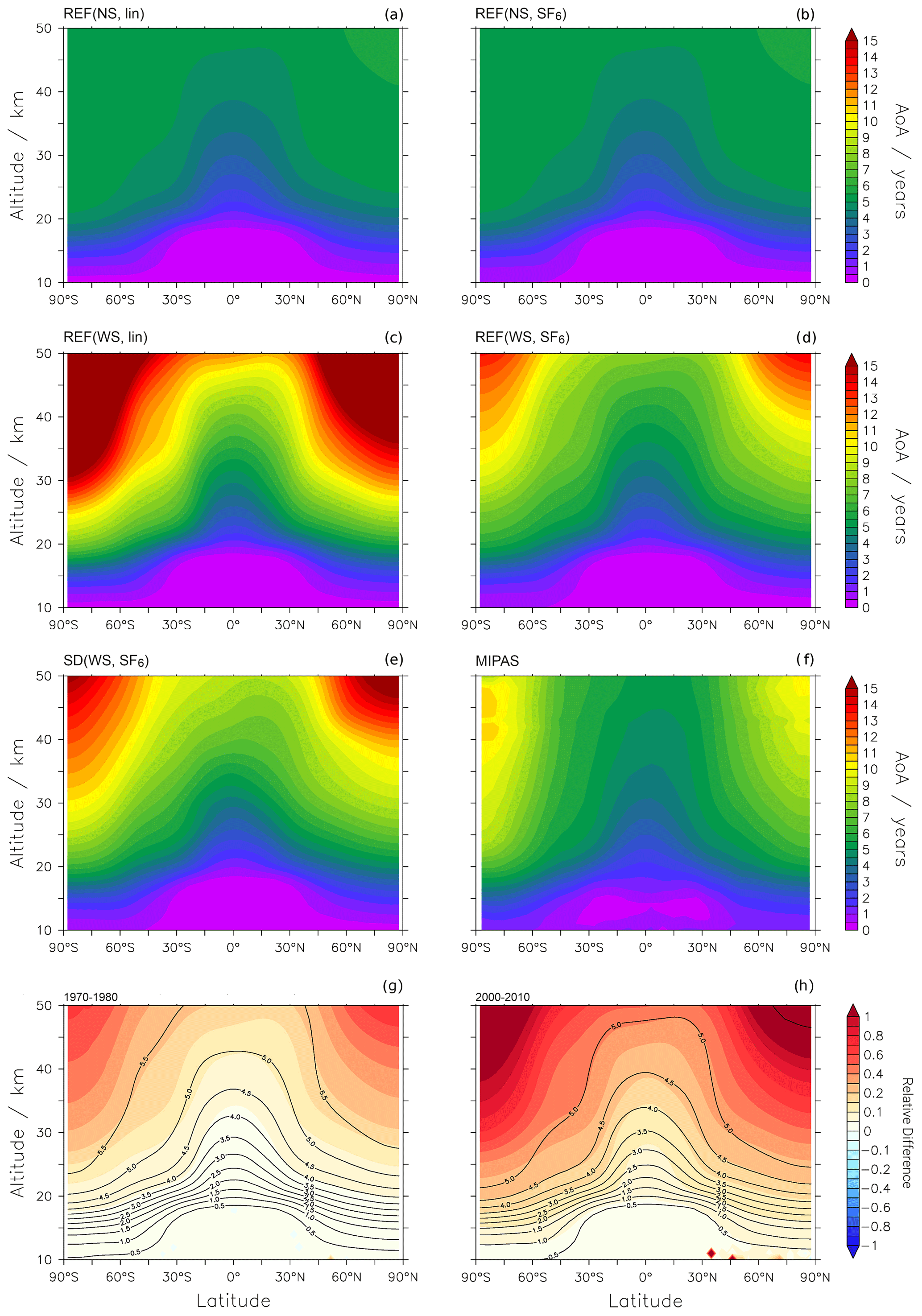
Figure 3 AoA climatologies of annual means over 2007–2010. Model AoA from the reference simulation for the different tracers, tr(NS, lin), tr(NS, SF₆), tr(WS, lin), and tr(WS, SF₆), is shown in panels (a)–(d), respectively, while AoA (tr(WS, SF₆)) from the specified dynamics simulation is shown in panel (e). MIPAS AoA (Stiller, 2021) can be seen in panel (f). The relative difference between AoA(WS, SF₆) and AoA(NS, SF₆) from the reference simulation for the 1970–1980 and 2000–2010 periods is shown in panels (g) and (h), respectively, and is calculated using $\frac{\text{AoA}(\text{WS},{\mathrm{SF}}_{\mathrm{6}})-\text{AoA}(\text{NS},{\mathrm{SF}}_{\mathrm{6}})}{\text{AoA}(\text{NS},{\mathrm{SF}}_{\mathrm{6}})}$ (where 1=100 %). The black contours depict AoA(NS, SF₆)_REF for the respective time period.

3.3 Age of air climatologies

AoA climatologies averaged over the period from 2007 to 2010 are shown in Fig. 3: from the reference simulation for REF(NS, lin), REF(NS, SF₆), REF(WS, lin), and REF(WS, SF₆) in Fig. 3a–d, respectively; from the specified dynamics simulation (SD(WS, SF₆)) in Fig. 3e; and from MIPAS SF₆ observations in Fig. 3f (Stiller, 2021). The years 2007 to 2010 were chosen as these are the only years with complete MIPAS data.

In all cases, AoA increases with increasing altitude and latitude. The cases considering sinks show an older apparent AoA than those without, especially with increasing altitude and latitude. This apparent aging can be explained by the fact that the inclusion of mesospheric sinks results in smaller SF₆ mixing ratios. The reduced mixing ratios lead to a seemingly older AoA as the corresponding reference value lies further in the past. Downwelling within the polar vortices transports old air from the mesosphere to the stratosphere. With the breakdown of the polar vortex at the end of the winter season, the old air is then mixed into lower latitudes. The relative effect of the sinks on AoA derived from the SF₆ tracers with nonlinear growth can be seen in Fig.  3g and h. Mean AoA values derived from SF₆ in the early period (1970–1980) are moderately affected by the sinks, with a difference of around 20 %–25 % in the polar middle stratosphere and above (i.e., for mean AoA values above 5.5 years). Differences are small (less than 10 %) for mean AoA values below 4 years. However, as will be discussed (see Sect. 3.5), the effect of the SF₆ sinks increases over time, and for the later period (2000–2010), mean AoA derived from SF₆ is considerably affected by the sinks. Differences greater than 20 % can be seen in Fig. 3h) for AoA above about 3 years, and in the extratropical lower stratosphere, differences are larger than 10 % even for mean AoA values of 2 years and above.

The patterns of modeled AoA from the linear tracers are similar to those of the SF₆-emission-based tracers (compare Fig. 3a with Fig. 3b and Fig. 3c with Fig. 3d). However, the similarities are weaker in the polar regions, especially when the SF₆ sinks are considered (Fig. 3c, d). In these regions, REF(WS, lin) reaches AoA values spanning 10–15 years or more, and REF(WS, SF₆) reaches AoA values of 9–14 years. This difference can be attributed to the greater initial growth of the tracer with linear emissions than that with nonlinear emissions (Fig. S2). This leads to enhanced SF₆ mixing ratios in the REF(WS, lin) case and, in turn, strengthens the influence of SF₆ sinks on AoA. This is particularly relevant in the winter months when SF₆-depleted mesospheric air is transported downward into the polar stratosphere.

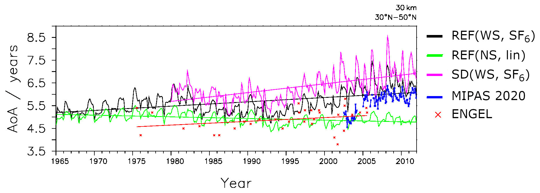
Figure 4 AoA time series and linear regressions calculated at 30 km averaged over 30–50^∘ N. EMAC AoA from SF₆ with nonlinear emissions from the reference simulations is shown in black (REF(WS, SF₆)). AoA from the tracer with linear emissions without sinks is shown in green (REF(NS, lin)). AoA from SF₆ with nonlinear emissions with sinks in the specified dynamics simulation SD(WS, SF₆) is shown in pink. AoA from balloon-borne measurements (Engel et al., 2009) and AoA from MIPAS observations (Stiller, 2021) are shown in red and dark blue, respectively.

AoA derived from SF₆ emissions including chemical SF₆ sinks (REF(WS, SF₆); Fig. 3d) agrees best with MIPAS AoA (Fig. 3f). Overall good agreement between EMAC and MIPAS AoA is found in the tropics, but there is a large high bias in the high latitudes in EMAC: between 40 and 50^∘ N, modeled AoA is up to 2 years older than MIPAS AoA in the stratosphere and up to 3 years older in the polar upper stratosphere (see Fig. S5 in the Supplement). In comparison to the MIPAS observations, the SF₆ sinks therefore seem to be too strong in the model, as already mentioned above. However, in comparison with the previously published MIPAS data (Stiller et al., 2012; Haenel et al., 2015), the EMAC AoA was actually too young (i.e., the MIPAS AoA was much older in the previous versions in the polar regions). The spectroscopic data used for the SF₆ retrieval in MIPAS cause a rather large bias (that has now been corrected by improved spectroscopy). The new spectroscopic data lead to a considerably younger AoA in the middle to upper stratosphere. There are, however, good reasons to believe that the most recent MIPAS data are improved compared with the previous ones: the spectroscopic data used are far better characterized than the previous ones (Harrison, 2020), and the new AoA data from MIPAS agree significantly better with independent measurements than the previous version, in particular at higher altitudes (Stiller et al., 2020; Stiller, 2021). On the other hand, free-running EMAC simulations generally have an overly weak Antarctic polar vortex (see Jöckel et al., 2016), which is, however, stronger than that of the reference simulation. Therefore, the more stable vortex in the SD simulation leads to enhanced isolation and aging of polar stratospheric air, especially in the Southern Hemisphere during austral spring (see Fig. S4 in the Supplement for details). This could somewhat resolve the issue for the comparison with the previous MIPAS AoA version (see Stiller et al., 2012, and Haenel et al., 2015, for further details); for the present MIPAS version, however, the discrepancies in the high altitudes and latitudes with the EMAC SD simulation are even larger than with the REF simulation. The comparison of Fig. 3e with Fig. 3f illustrates that the model cannot reproduce the tropical pipe and exhibits too much horizontal mixing, or overly slow upwelling. This could explain why the model does not reproduce the constant AoA with height in the midlatitudes. A detailed assessment of both the satellite data and the model simulations is necessary to resolve these discrepancies. In the model, dynamical effects like the strength of the polar vortex or the gravity wave parameterization can play important roles in the downwelling strength. Moreover, various processes of chemical SF₆ removal can be revised and/or parameterized differently. Here, we showed that SF₆ sinks have the potential to resolve the differences between simulated and observed climatologies of AoA and that EMAC AoA lies within the uncertainties of MIPAS AoA throughout the atmosphere. Therefore, we consider our simulations suitable for studying the temporal evolution of AoA.

3.4 Apparent age of air trends

In this section, we analyze the EMAC AoA trends and compare them with observation-based AoA trends. Figure 4 shows the AoA time series and linear regressions from the REF and the SD simulations as well as from MIPAS observations (Stiller, 2021) and from the SF₆ measurements by Engel et al. (2009). As the latter were collected from balloon flights in the Northern Hemisphere midlatitudes at around 30 km altitude, the EMAC and MIPAS data are also taken from that height and averaged over 30–50^∘ N for consistency.

Engel et al. (2009)

Table 3 EMAC AoA trends at 30 km averaged over 30–50^∘ N. The calculation of the 2002–2011 trends is provided for the two relevant simulations, REF(WS, SF₆) and SD(WS, SF₆), and follows the methods used in Haenel et al. (2015). The 2002–2011 trends are also provided for the remaining simulations.

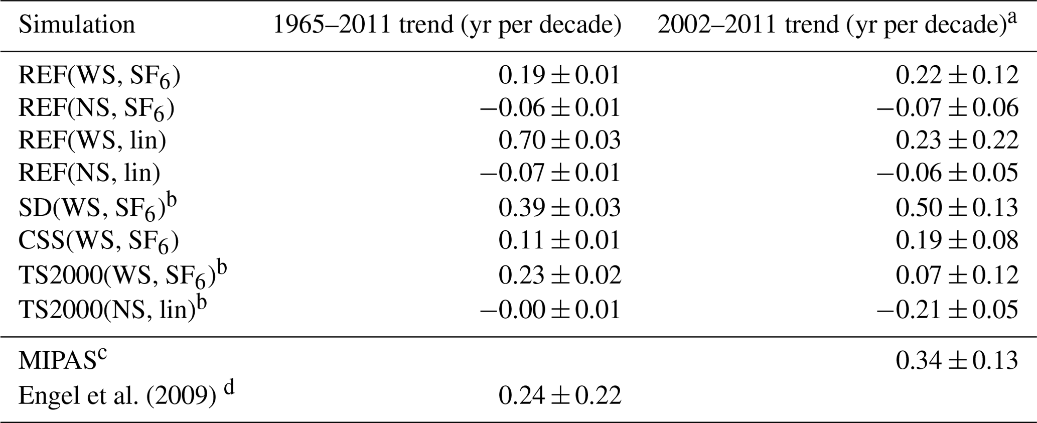
^a Trend calculated following methods of Haenel et al. (2015). ^b Trend calculated over 1980–2011 at 30 km altitude. ^c MIPAS trend calculated over 2002–2012. ^d Trend calculated over 1975–2005 between 32 and 51^∘ N and between 24 and 35 km.

For better quantification of the trends, Table 3 provides the AoA trend values of the EMAC simulations for two periods. The trend in the entire simulation period from 1965 to 2011 is taken for long-term trend assessment and comparison with the measurements by Engel et al. (2009). For the comparison with MIPAS data, the EMAC AoA trends are shown for the 2002–2011 period between 30 and 50^∘ N, for the realistic tracer tr(WS, SF₆). The trend calculation follows that of Haenel et al. (2015).

The tracers without SF₆ sinks lead to negative AoA trends, which are consistent with the simulated acceleration of the BDC in the course of climate change (e.g., Garcia and Randel, 2008). Positive AoA trends are obtained for all tracers that take SF₆ chemistry into account. The trend of 0.19 ± 0.01 yr per decade in the REF simulation (WS, SF₆) is within the limits of the uncertainties of the trend obtained by Engel et al. (2009), who calculated an AoA trend of 0.24 ± 0.22 yr per decade. This means that, in our simulations, the sinks help to reconcile the modeled and the measured AoA trends over the recent decades. Note that Engel et al. (2009, 2017) also obtained a positive trend for AoA derived from CO₂ measurements.

Haenel et al. (2015) calculated MIPAS AoA trends for the period from 2002 to 2012 of 0.25 ± 0.11 yr per decade for 30–40^∘ N at 30 km and of 0.24 ± 0.11 yr per decade for 40–50^∘ N at 30 km. For the new MIPAS dataset, the AoA trend is 0.34 ± 0.13 yr per decade. Note that these trends are calculated by applying a bias correction for the discontinuity between the two different observational periods of MIPAS (see Fig. 4); a description of the method can be found in von Clarmann et al. (2010).

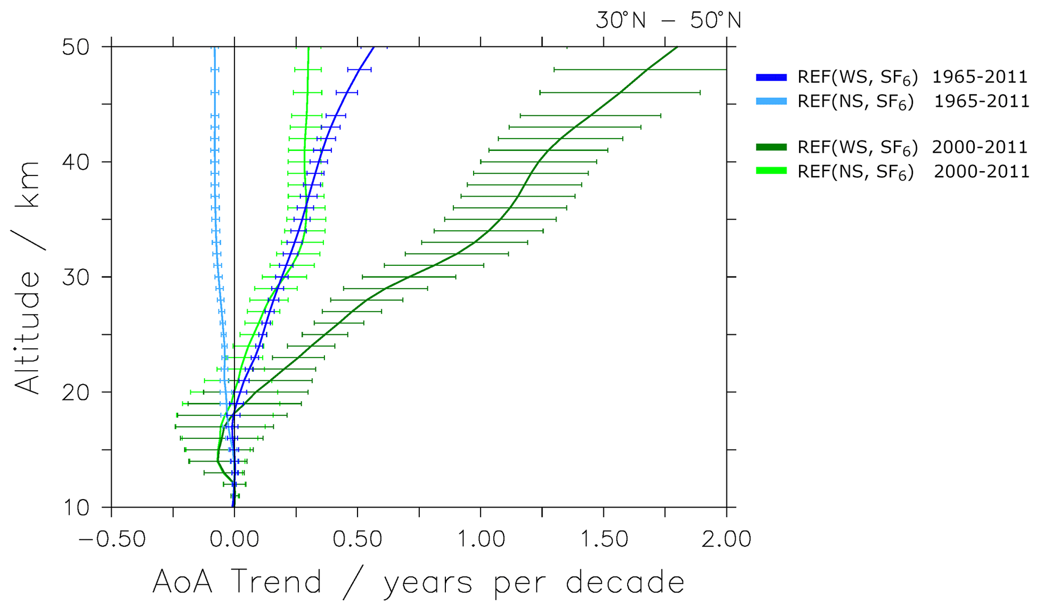
Figure 5 Vertical profile of the linear trends of AoA(WS, SF₆)_REF and AoA(NS, SF₆)_REF over 30–50^∘ N, calculated for the 1965–2011 and 2000–2011 time periods. Error bars depict the 2σ standard deviation of the trend over the respective time period, and the black vertical line denotes the zero line.

Following the trend calculation used in Haenel et al. (2015), the REF(WS, SF₆) and SD(WS, SF₆) time series show that EMAC AoA bears a good resemblance to that of the new MIPAS retrieval, with an AoA trend of 0.22 ± 0.12 and 0.50 ± 0.13 yr per decade, respectively. Consistent with the trend calculation of the MIPAS data, the variability due to the QBO is considered by a respective term in the multivariate linear analysis. However, this measure induces only small differences in the EMAC trend calculations (see Table S1 in the Supplement for further details). Note also that the rather short period of the MIPAS observations implies rather large uncertainties in the trends because interannual variability can have a large effect on the trend calculations. This is also apparent from the highly variable trend signals in the different simulations; for example, the TS2000(NS, lin) exhibits a strongly negative trend over this period despite no forced long-term trends. This is confirmed by a trend of −0.00 ± 0.01 yr per decade over the 1965–2011 period.

Figure 6 AoA (at 10 hPa, averaged over 30–50^∘ N) time series and linear regression of sensitivity experiments TS2000(WS, SF₆), TS2000(NS, lin), and CSS(WS, SF₆) shown in dark blue, light blue, and pink, respectively. The reference simulations REF(WS, SF₆) and REF(NS, lin) are shown in black and green, respectively.

As shown in Fig. 5, the strong deviation of SF₆-derived AoA trends holds almost throughout the stratosphere. Only below about 20 km altitude for the period from 1965 to 2011 are the effects of the SF₆ sinks smaller than the trend uncertainty. For the trend in the shorter time period of 2000–2011, effects from the SF₆ sinks become significant at about 22 km altitude and higher, which is mainly due to the larger uncertainty stemming from a smaller time period. This means that the SF₆-based AoA trends with and without sinks are not distinguishable from each other up to 20 and 22 km altitude in the midlatitudes, depending on the period. Furthermore, the uncertainty in the trend calculated from SF₆-based AoA with sinks increases with increasing altitude – this is to be expected, as the effect of the SF₆ sinks increases with increasing altitude. The trend in AoA(NS,SF₆)_REF over the 2000–2011 period is positive at 25 km and negative over the longer 1965–2011 period. However, it is important to note that the time period of about 1 decade implies that the trend is strongly influenced by interannual variability (see, e.g., Dietmüller et al., 2021). The strong influence of interannual variability also explains the difference in trend values in Fig. 5, for which trends are calculated with a simple linear fit, versus the value for a similar period in Table 3. The latter trends were calculated using a regression model taking other variability modes into account to enable a comparison with MIPAS.

3.5 Explanations of apparent age of air trends

In this section, we will analyze the EMAC apparent AoA trends, in particular the sign change of the trend when SF₆ sinks are switched on. For this, Fig. 6 shows the AoA (WS,SF₆) time series of the sensitivity simulations CSS and TS2000 averaged between 30 and 50^∘ N. For comparison, AoA values from the reference simulation (REF(WS, SF₆) and REF(NS, lin)) are also included.

In the CSS simulation, the mixing ratios of the reactant species involved in the sink reactions of SF₆ are held constant. The CSS simulation with the realistic tracer (CSS(WS, SF₆)) shows an AoA trend of 0.11 ± 0.01 yr per decade over the 1965–2011 period. This is lower than the AoA trend in the reference simulation REF(WS, SF₆) and means that while the changes in the SF₆-depletive substances influence the magnitude of the positive trend, they cannot explain the positive sign of the AoA trend.

The TS2000 simulation is a time slice simulation with climate conditions of the year 2000. AoA of that simulation derived from the realistic tracer (TS2000(WS, SF₆)) shows a positive trend of 0.23 ± 0.02 yr per decade. This is even stronger than the trend in the REF simulation (0.19 ± 0.01 yr per decade). By definition, the TS2000 simulation does not feature any changes in its climatic state nor in the composition of the atmosphere. This is reflected by the fact that the idealized tracer tr(NS, lin) does not show a trend in this simulation (see Table 3; TS2000(NS, lin): −0.00 ± 0.01). The temporal increase in apparent AoA rise in the TS2000(WS, SF₆) simulation despite no climate changes therefore points to the fact that the SF₆ sinks themselves lead to the positive trend. The difference between the TS2000 and the REF AoA trends for both tr(WS, SF₆) and tr(NS, lin) reflect the negative contribution of the accelerating BDC to the trend, which can be seen in the idealized AoA trend from the REF simulation (NS, lin). Overall, neither changes in the SF₆ sinks nor changes in the stratospheric circulation due to climate change are responsible for the positive trend found in AoA with sinks. Instead, the results indicate that the sinks themselves can generate a positive trend.

For a complete discussion of the features that can be seen in Fig. 6, we now also describe the sudden decrease in AoA(WS, SF₆) shortly after 1982 seen in the REF simulation. It is also visible in the two sensitivity simulations (CSS and TS2000). This means that changes in the SF₆-depleting substances as well as climate change and volcanic activity (in particular the volcanic eruption of El Chichón in 1982) can be ruled out as possible causes of the drop. The solar cycle is not taken into account in the time slice simulation. The time series of the realistic SF₆ tracer emissions show a stronger increase in the 1980s (not shown). Fritsch et al. (2020) showed that, due to this increase, the calculation of AoA based on SF₆-like tracers is more sensitive to the chosen parameters in the AoA derivation for this time. The drop in AoA that we see is caused by this limitation of the derivation from SF₆-like tracers.

The increasing variability and trend in AoA in the last 2 decades, seen in the simulations with mesospheric SF₆ chemistry, can be attributed at first order to the SF₆ depletion reactions (see Fig. 6). In particular, the effect of mesospheric SF₆ sinks is stronger with higher SF₆ mixing ratios. Subsequent downward transport of SF₆-depleted air into the vortex and in-mixing thereof into lower latitudes after the vortex breakup results in apparent older AoA. This can explain that the annual variability increases over time due to the increase in SF₆ mixing ratios.

4 Theoretical considerations and concept for sink correction methods

The following section focuses on the theoretical examination of the link between SF₆ sinks and positive AoA trends. First, we will show, from a theoretical standpoint, that SF₆ sinks with constant destruction rates lead to a positive trend in AoA. Based on the theoretical considerations and on the model data, we will then discuss the possibilities of a correction of AoA derived from SF₆ data for the effects of the sinks. Many observational mean AoA estimates are based on measurements of SF₆, and given that the relevance of the sinks of the mean AoA estimates increases over time, a correction method is required to obtain unbiased information on stratospheric transport strengths.

The aforementioned link between the positive AoA trend and mesospheric SF₆-depletive chemistry, based on Hall and Waugh (1998), is illustrated below and follows the mathematical formulations put forward by Hall and Plumb (1994) and Schoeberl et al. (2000). To allow for analytical expressions, we will only consider the case of a linearly increasing tracer here, and we will further assume that the lifetime of SF₆ is constant in time. We consider a tracer χ(t) experiencing relative loss $e^{-t/\mathit{\tau }}$ with time-constant lifetime τ. Note that τ is equivalent to the inverse of the loss rate. We denote the reference mixing ratio as χ_o(t) and assume a constant growth rate of Δχ_oo:

$$\begin{array}{}\text{(3)}& {\mathit{\chi }}_{\mathrm{o}}\left(t\right)=\mathrm{\Delta }{\mathit{\chi }}_{\text{oo}}\cdot t.\end{array}$$

For any location, we can then express the tracer mixing ratio as

$$\begin{array}{}\text{(4)}& \mathit{\chi }\left(t\right)=\underset{t^{\prime }=\mathrm{0}}{\overset{\mathrm{\infty }}{\int }}{\mathit{\chi }}_{\mathrm{o}}(t-t^{\prime })\cdot e^{(-t^{\prime }/\mathit{\tau })}\cdot G\left(t^{\prime }\right)\mathrm{d}{t}^{\prime },\end{array}$$

where t^′ denotes the transit time; G(t^′) represents the Green's function and is equivalent to the AoA spectrum. Inserting Eq. (3) into Eq. (4) gives us

$$\begin{array}{}\text{(5)}& \begin{array}{rl}\mathit{\chi }\left(t\right)=& \mathrm{\Delta }{\mathit{\chi }}_{\text{oo}}\cdot t\underset{t^{\prime }=\mathrm{0}}{\overset{\mathrm{\infty }}{\int }}{e}^{(-t^{\prime }/\mathit{\tau })}\cdot G\left(t^{\prime }\right)\mathrm{d}{t}^{\prime }\\ & -\mathrm{\Delta }{\mathit{\chi }}_{\text{oo}}\underset{t^{\prime }=\mathrm{0}}{\overset{\mathrm{\infty }}{\int }}{t}^{\prime }{e}^{(-t^{\prime }/\mathit{\tau })}\cdot G\left(t^{\prime }\right)\mathrm{d}{t}^{\prime }.\end{array}\end{array}$$

The expression under the first integral corresponds to the arrival time distribution $G^{\ast }\left(t^{\prime }\right)=\exp (-t^{\prime }/\mathit{\tau })G\left(t^{\prime }\right)$. This represents the transit time distribution of a chemically depleted tracer with lifetime τ (see, e.g., Plumb et al., 1999; however, note that G^∗ is not normalized in our definition, following Engel et al., 2017). Note that τ is a measure of the lifetime an air parcel experiences on its path of length t^′ and is referred to the path-integrated lifetime (not to be confused with the local lifetime). The second integral in Eq. (5) is the first moment of the arrival time distribution $G^{\ast }\left(t^{\prime }\right)$ (i.e., the mean arrival time and is denoted as Γ^∗). Using these terms, Eq. (5) can be expressed as

$$\begin{array}{}\text{(6)}& \mathit{\chi }\left(t\right)=\mathrm{\Delta }{\mathit{\chi }}_{\text{oo}}\left(t\cdot \underset{t^{\prime }=\mathrm{0}}{\overset{\mathrm{\infty }}{\int }}{G}^{\ast }\left(t^{\prime }\right)\mathrm{d}{t}^{\prime }-{\mathrm{\Gamma }}^{\ast }\right).\end{array}$$

For the tracer without sinks (here referred to as the passive tracer χ_p(t)), the integral over $G^{\ast }\left(t^{\prime }\right)$ equals 1, and Γ represents the mean AoA. Equation 6 can then be rearranged to

$$\begin{array}{}\text{(7)}& \mathrm{\Gamma }=t-{\displaystyle \frac{{\mathit{\chi }}_p\left(t\right)}{\mathrm{\Delta }{\mathit{\chi }}_{\text{oo}}}},\end{array}$$

giving the common expression to derive mean AoA from a linear increasing tracer.

In the case of a tracer with sinks, χ_s(t), the calculation of (apparent) mean AoA based on Eqs. (6) and (7) becomes

$$\begin{array}{}\text{(8)}& \begin{array}{rl}\stackrel{\mathrm{̃}}{\mathrm{\Gamma }}& =t-{\displaystyle \frac{{\mathit{\chi }}_s\left(t\right)}{\mathrm{\Delta }{\mathit{\chi }}_{\text{oo}}}}=t-\left(t\cdot \underset{t^{\prime }=\mathrm{0}}{\overset{\mathrm{\infty }}{\int }}{G}^{\ast }\left(t^{\prime }\right)\mathrm{d}{t}^{\prime }+{\mathrm{\Gamma }}^{\ast }\right)\\ & =t\left(\mathrm{1}-\underset{t^{\prime }=\mathrm{0}}{\overset{\mathrm{\infty }}{\int }}{G}^{\ast }\left(t^{\prime }\right)\mathrm{d}{t}^{\prime }\right)+{\mathrm{\Gamma }}^{\ast }.\end{array}\end{array}$$

The change of apparent mean AoA with time can then be expressed as

$$\begin{array}{}\text{(9)}& {\displaystyle \frac{\partial \stackrel{\mathrm{̃}}{\mathrm{\Gamma }}}{\partial t}}=\mathrm{1}-\underset{t^{\prime }=\mathrm{0}}{\overset{\mathrm{\infty }}{\int }}{G}^{\ast }\left(t^{\prime }\right)\mathrm{d}{t}^{\prime }.\end{array}$$

In the case of a passive tracer (i.e., a tracer without sinks), $G^{\ast }\left(t^{\prime }\right)$ is equal to the age spectrum G(t^′); thus, its integral equals 1. Consequently, the AoA trend is zero in the absence of a trend in transport (constant G). However, for the depleted tracer (with sinks), a positive linear trend in the apparent mean AoA ($\stackrel{\mathrm{̃}}{\mathrm{\Gamma }}$) is induced by the sinks, even if the circulation strength (i.e., G(t^′)) and the lifetimes τ(t^′) are constant. This is consistent with the results shown in the previous sections. In particular, we showed a positive trend in the linearly increasing SF₆-like tracer in the time slice experiment (TS2000, see, e.g., Table 2), which satisfies all of the conditions made above. In the reference simulation, the BDC is accelerating over time, so that mean AoA from the passive tracer is decreasing. However, in our simulations, the positive trend induced by the sinks overcompensates for the impact of the BDC acceleration. It is important to note that the above is valid for a linearly increasing tracer and that variable growth rates will modify the influence of SF₆ on apparent AoA.

A correction of the mean AoA estimate for the effects of the sinks would require knowledge of the (integrated) arrival time distribution G^∗ (or, equivalently, the transit-time-dependent path-integrated lifetimes τ(t^′)), a quantity that is not readily available and possibly nonlinearly dependent on Γ. As a thought experiment, with the aim of deriving an analytical concept for the correction of mean AoA for the sinks, we make the hypothetical assumption that the age spectrum is represented by a single, average path (i.e., we assume the age spectrum is a delta function $G\left(t^{\prime }\right)=\mathit{\delta }\left(\mathrm{\Gamma }\right)$). With this assumption, the tracer mixing ratio of the depleted tracer (Eq. 5) simplifies to

$$\begin{array}{}\text{(10)}& {\mathit{\chi }}_s\left(t\right)=\mathrm{\Delta }{\mathit{\chi }}_{\text{oo}}\cdot e^{-\frac{\mathrm{\Gamma }}{{\mathit{\tau }}_{\text{eff}}}}\cdot (t-\mathrm{\Gamma }),\end{array}$$

where τ_eff is the path-integrated lifetime along this single path. To avoid confusion with either the local lifetime or the averaged transit-time-dependent path-integrated lifetime, we will refer to τ_eff as the “effective” lifetime.

The apparent mean AoA calculated from the depleted tracer χ_s(t) follows from Eqs. (7) and (10):

$$\begin{array}{}\text{(11)}& \stackrel{\mathrm{̃}}{\mathrm{\Gamma }}=t-{\displaystyle \frac{{\mathit{\chi }}_s\left(t\right)}{\mathrm{\Delta }{\mathit{\chi }}_{\text{oo}}}}=t\left(\mathrm{1}-e^{-\frac{\mathrm{\Gamma }}{{\mathit{\tau }}_{\text{eff}}}}\right)+e^{-\frac{\mathrm{\Gamma }}{{\mathit{\tau }}_{\text{eff}}}}\cdot \mathrm{\Gamma }.\end{array}$$

Given that the mean age Γ is about 2 orders of magnitude lower than the lifetime τ_eff, we can approximate $e^{-\frac{\mathrm{\Gamma }}{{\mathit{\tau }}_{\text{eff}}}}\approx \mathrm{1}-\frac{\mathrm{\Gamma }}{{\mathit{\tau }}_{\text{eff}}}$; thus, $\stackrel{\mathrm{̃}}{\mathrm{\Gamma }}=\mathrm{\Gamma }(\mathrm{1}+\frac{t}{{\mathit{\tau }}_{\text{eff}}})-\frac{{\mathrm{\Gamma }}^{\mathrm{2}}}{{\mathit{\tau }}_{\text{eff}}}$. Again for small Γ compared with τ_eff, the second term can be neglected so that

$$\begin{array}{}\text{(12)}& \stackrel{\mathrm{̃}}{\mathrm{\Gamma }}\approx \mathrm{\Gamma }\left(\mathrm{1}+{\displaystyle \frac{t}{{\mathit{\tau }}_{\text{eff}}}}\right).\end{array}$$

In general, τ_eff will be dependent on Γ. However, if the effective lifetime were constant, the apparent mean age $\stackrel{\mathrm{̃}}{\mathrm{\Gamma }}$ would be linearly related to the actual mean AoA. The slope between the latter two then is merely a function of the effective lifetime and increases linearly over time t. Thus, for constant circulation (Γ) and effective lifetime τ_eff, a linear trend in strength

$$\begin{array}{}\text{(13)}& {\displaystyle \frac{\partial \stackrel{\mathrm{̃}}{\mathrm{\Gamma }}}{\partial t}}=\mathrm{1}+e^{-\frac{\mathrm{\Gamma }}{{\mathit{\tau }}_{\text{eff}}}}\approx {\displaystyle \frac{\mathrm{\Gamma }}{{\mathit{\tau }}_{\text{eff}}}}\end{array}$$

is induced.

Under these assumptions, a relatively simple, linear relation between the true mean AoA (Γ) and the apparent AoA ($\stackrel{\mathrm{̃}}{\mathrm{\Gamma }}$) is obtained. While the assumptions will clearly be violated in the model, we investigate, based on data from our model simulations, whether the violations might effectively be small enough so that the linear relation still holds. In particular, the linearly increasing tracers from the time slice simulation (TS2000) with constant circulation strength satisfy the initial assumptions (linear increase and constant circulation), and we can test whether the approximations of a single average path hold.

Figure 7 Midlatitude (30–50^∘ N) averaged mean AoA from the ideal tracer plotted against the apparent mean AoA derived from the linearly increasing SF₆-like tracer from the TS2000 simulations, for years ranging from year 1 (yellow) to year 40 (dark red). Panel (b) shows the same as panel (a) but is limited to ages below 5 years. The gray lines are estimations based on Eq. (11) for t = 40 years, with either a constant effective lifetime of 140 years (dashed) or with the effective lifetime dependent on Γ (as shown in Fig. 8).

Figure 7 shows a quasi-linear relation between the ideal AoA and AoA derived from the linearly increasing SF₆-like tracer for mean AoA values below approximately 4 years. The slope increases over time (as apparent from the transition from yellow to red colors in Fig. 7), consistent with the simplified theoretical considerations for a constant effective lifetime τ_eff (see Eq. 12). However, for mean AoA values above about 5 years, this quasi-linear regime does not hold anymore. We instead find exponential growth of SF₆-based apparent mean AoA. Those older mean AoA values are closer to the region of depletion in the mesosphere, and a constant effective lifetime (as assumed for the linear regime) does not hold anymore. Rather, we can expect τ_eff to be strongly dependent on Γ.

Figure 8 Effective lifetime derived from average midlatitude (30–50^∘ N) ideal mean AoA and apparent mean AoA (from the linearly increasing SF₆-like tracer) from the TS2000 simulations. The calculation of τ_eff is based on Eq. (11) (blue solid line) and its linear approximation Eq. (12) (black dashed line).

Based on Eq. (11) (or its linear approximation Eq. 12), we can estimate the effective lifetime from the model data of Γ (from the passive tracer) and $\stackrel{\mathrm{̃}}{\mathrm{\Gamma }}$ (from the linearly increasing SF₆-like tracer). The resulting lifetime is shown in Fig. 8 as a function of the ideal mean AoA. Consistent with the previous results, τ_eff varies comparatively little with Γ for a range between 1 and 4 years. Figure 7 also includes the theoretical values of $\stackrel{\mathrm{̃}}{\mathrm{\Gamma }}$ according to Eq. (11) for t = 40 years and when using either a constant mean value for τ_eff of 140 years (obtained for Γ = 3.3 years) or the Γ-dependent values. The approximation of a constant effective lifetime matches the model data for ages below about 4 years reasonably well, but for older air, the assumption of a constant τ_eff obviously fails. When using the Γ-dependent value for τ_eff, on the other hand, the exponential increase in $\stackrel{\mathrm{̃}}{\mathrm{\Gamma }}$ is generally well captured. This justifies the applicability of the simplified assumptions of one average path (Eqs. 11, 12).

Overall, the results derived in this section indicate that a correction of observational SF₆-derived mean AoA for the effects of chemical sinks is likely possible by applying a time-dependent linear correction function. This linear relation between AoA from the ideal and from the chemically depleted SF₆ tracer holds for mean ages below about 4 years. Here, we show this relation for the linearly increasing tracer in northern midlatitudes. However, further analysis indicates that this linear relation also holds for the realistic SF₆ tracer with nonlinear growth over time (not shown). Furthermore, the linear relation seems to be nearly identical for different latitude bands (not shown), which is a very promising property for future applications of a correction method.

We emphasize that the strength of the SF₆ sink in our model simulations is not well enough constrained to properly establish such a correction function. Deriving suitable values for the linear relation between Γ and $\stackrel{\mathrm{̃}}{\mathrm{\Gamma }}$ (and, thus, the effective lifetime τ_eff) should be obtained by means of observational data. This could be achieved by using simultaneous measurements of SF₆ and other age tracers, as previously shown by Leedham Elvidge et al. (2018) and Adcock et al. (2021). Furthermore, the concept needs to be evaluated vigorously on model data to assess its errors and limitations.

5 Summary and conclusions

For over a decade, disagreements with regards to stratospheric AoA and, particularly, its trends between model simulations and observations have raised many questions from scientists. AoA from observations is mostly older than AoA from model simulations, and models simulate a decrease in AoA over recent decades, whereas trend estimates from observational data report a nonsignificant positive trend. In agreement with our results, previous studies (see, e.g., Kouznetsov et al., 2020) have shown that the chemical sinks strongly influence SF₆-derived AoA in terms of absolute values and decadal changes. We investigate, for the first time, how longer-term trends are affected in a consistent manner, and we explore the different contributions from circulation changes, changes in abundance of reaction partners, and trends induced by constant destruction rates. Thus, to make this step towards understanding the reasons for the discrepancies, we study the impact of mesospheric SF₆ sinks on AoA climatologies and trends using the chemistry climate model EMAC (Jöckel et al., 2010, 2016) with the SF6 submodel (Reddmann et al., 2001). This submodel allows for explicit calculation of SF₆ sinks, and we applied a correction for the nonlinear growth of SF₆ in the calculation of AoA (Fritsch et al., 2020).

The EMAC SF₆ mixing ratio profiles show good agreement with balloon-borne measurements as well as with satellite observations. Some of the differences between the model and observations are within the uncertainty range of the observations. However, reasons for the quantitative differences in the high latitudes and altitudes can also be found in deficiencies in the representation of the SF₆ sinks in the model or in the dynamics simulated by the model. The EMAC reference simulation yields a global stratospheric SF₆ lifetime of 2100 years, varying between 2500 and 1900 years for the simulation period. This value lies within the range of 600–2900 years provided by the model study of Kouznetsov et al. (2020) and below the value 3200 years calculated by Ravishankara et al. (1993). Kovács et al. (2017) and Ray et al. (2017) recently found somewhat lower SF₆ lifetimes of 1278 and 850 years, respectively. Although this shows that large uncertainties still exist in determining the SF₆ lifetime, these results also confirm that the EMAC SF₆ depletion mechanisms are reasonable. In our transient simulations (REF and PRO), the SF₆ lifetimes vary by about 25 % following the abundances of the reactant species, basically resembling the pattern of the stratospheric ozone concentration. This behavior, however, may be a result of the fact that several effects that potentially influence SF₆ lifetime variability are not implemented in full detail.

The inclusion of SF₆ sinks translates into apparent older stratospheric air; thus, when SF₆ sinks are enabled, EMAC AoA compares better with MIPAS satellite observations. In the tropics, good agreement can generally be found, but the results also indicate that EMAC does simulate an overly broad, less-isolated tropical pipe. In polar regions, however, EMAC AoA is higher than MIPAS AoA. In comparison with the previously published MIPAS data (Stiller et al., 2012; Haenel et al., 2015), the EMAC AoA in the polar regions was actually too low. More research on both models and observations is necessary to resolve these remaining discrepancies.

In this study, we show the effect of SF₆ sinks on the tracer-derived AoA trend for both longer time series as well as for the short time series corresponding to the MIPAS time frame, although issues in variability are associated with the latter. Without SF₆ sinks, EMAC shows a negative AoA trend over 1965–2011. This is consistent with the simulated acceleration of the Brewer–Dobson circulation resulting from climate change (see, e.g., Garcia and Randel, 2008, Butchart et al., 2011, and Eichinger et al., 2019). The inclusion of chemical SF₆ sinks leads to positive AoA trends throughout the stratosphere (except the tropical lower stratosphere below 50 hPa) in our simulations, which, in turn, is consistent with the positive AoA trend derived from MIPAS in the Northern Hemisphere (Haenel et al., 2015). Moreover, the SF₆ sinks help to improve the agreement of our model results with the AoA derived from the balloon-borne in situ measurements by Engel et al. (2009), from which a (nonsignificant) positive AoA trend was obtained. However, this only accounts for SF₆-derived AoA, and our results cannot help explain the positive trend in the CO₂-derived AoA in Engel et al. (2009, 2017). Furthermore, it has recently been shown that the AoA trend derived in Engel et al. (2009, 2017) was likely overestimated due to nonideal parameter choices in the calculation of AoA (Fritsch et al., 2020).

Our sensitivity studies quantified that the positive AoA trends are neither a result of climate change nor of changes in the substances involved in SF₆ depletion. The SF₆ sinks themselves are the reason for the increase in apparent AoA. The reason for that is the temporally increasing influence of the chemical SF₆ sinks on AoA. In our simulations, this effect overcompensates for the effect of the simulated acceleration of the stratospheric circulation, leading to a net increase in AoA. Due to various sources of uncertainties, this result bears quantitative leeway and has to be assessed in finer detail. Nevertheless, for now, we can conclude that SF₆ sinks have the potential to explain the long-lasting AoA trend discrepancies between models and observations. Furthermore, we put forward a first approach towards a method for SF₆ loss correction, which shall be further developed and applied on observational data in the future. From our first analyses, we can conclude that a linear correction (that is dependent on both time and the effective lifetime of SF₆) can likely be applied to AoA values up to 4 years. However, further studies with more comprehensive approaches are required for a precise quantification of these values.