the Creative Commons Attribution 4.0 License.
the Creative Commons Attribution 4.0 License.
 | 07 Sep 2022
Quantifying NOx emissions in Egypt using TROPOMI observations
Anthony Rey-Pommier
Frédéric Chevallier
Philippe Ciais
Grégoire Broquet
Theodoros Christoudias
Jonilda Kushta
Didier Hauglustaine
Jean Sciare
Urban areas and industrial facilities, which concentrate the majority of human activity and industrial production, are major sources of air pollutants, with serious implications for human health and global climate. For most of these pollutants, emission inventories are often highly uncertain, especially in developing countries. Spaceborne measurements from the TROPOMI instrument, on board the Sentinel-5 Precursor satellite, are used to retrieve nitrogen dioxide (NO2) column densities at high spatial resolution. Here, we use 2 years of TROPOMI retrievals to map nitrogen oxide (NOx = NO + NO2) emissions in Egypt with a top-down approach using the continuity equation in steady state. Emissions are expressed as the sum of a transport term and a sink term representing the three-body reaction comprising NO2 and hydroxyl radical (OH). This sink term requires information on the lifetime of NO2, which is calculated with the use of the CAMS near-real-time temperature and OH concentration fields. We compare this derived lifetime with the lifetime inferred from the fitting of NO2 line density profiles in large plumes with an exponentially modified Gaussian function. This comparison, which is conducted for different samples of NO2 patterns above the city of Riyadh, provides information on the reliability of the CAMS near-real-time OH concentration fields; it also provides some hint on the vertical levels that best represent typical pollution sources in industrial areas and megacities in the Middle East region. In Egypt, total emissions of NOx are dominated by the sink term, but they can be locally dominated by wind transport, especially along the Nile where human activities are concentrated. Megacities and industrial regions clearly appear as the largest sources of NOx emissions in the country. Our top-down model infers emissions with a marked annual variability. By looking at the spatial distribution of emissions at the scale of different cities with different industrial characteristics, it appears that this variability is consistent with national electricity consumption. We detect lower emissions on Fridays, which are inherent to the social norm of the country, and quantify the drop in emissions in 2020 due to the COVID-19 pandemic. Overall, our estimations of NOx emissions for Egypt are 7.0 % higher than the CAMS-GLOB-ANT_v4.2 inventory and significantly differ in terms of seasonality.
- Article
(5190 KB) - Full-text XML
- BibTeX
- EndNote


Economic growth in developing countries has led to a strong increase in urban air pollution (Baklanov et al., 2016). Among the different pollutants, nitrogen oxides are key species. They are generally the products of fuel combustion, such as the burning of hydrocarbons in the air at high temperature. The main sources of these compounds are vehicle engines, but also heavy industrial facilities such as power plants, iron and steel mills (Tang et al., 2020), and cement kilns (Kim et al., 2020). Their accumulation in the lowest layers of the troposphere contributes to the formation of smog and acid rain (Singh and Agrawal, 2008). They also have a significant effect on human health, as they can cause various respiratory diseases (EPA, 2016). To deal with these phenomena, national and regional governments generally enact a series of air pollution control strategies, which typically take the form of bans on certain polluting technologies, with the aim of reducing the concentration of pollutants at the local level to targets that must be achieved within a given timeframe. These strategies, which also help drive technological innovation, have had a significant effect in Europe (Crippa et al., 2016).
In Egypt, population growth, urbanisation, socio-economic development and the associated increase in the vehicle fleet led to a major degradation of air quality in the last decades, especially in highly populated areas such as Greater Cairo and the Nile Delta (El-Magd et al., 2020), which include the majority of the population. The Ministry of State for the Environment has thus initiated new policies that aim to reduce pollution levels throughout the country, through technical mitigation of emissions, emission standards for vehicles and intersectoral collaboration (UNEP, 2015). However, Egypt, like most developing countries, lacks the local infrastructure to access detailed information on technical factors such as energy consumption or fuel type and technology, leading to discrepancies in inventories (Xue and Ren, 2012). As a consequence, the monitoring of emissions, which is important to evaluate the effects of air pollution control policies, is of limited reliability.
To overcome the uncertainties in the emission inventories, the use of independent observation systems is becoming increasingly prevalent. In this study, we investigate the use of satellite remote sensing of atmospheric concentrations to improve the quantification of NOx emissions in Egypt. Spectrally resolved satellite measurements of solar backscattered radiation enable the quantification of NO2 and other trace gases absorbing in the UV–visible spectral range based on their characteristic spectral absorption patterns. Tropospheric vertical column densities, i.e. vertically integrated NO2 concentrations in the troposphere, have been providing information on the spatial distribution of tropospheric NO2 at a global scale for nearly 30 years, allowing the identification of different sources of NOx and the quantification of the associated emissions (Leue et al., 2001; Martin et al., 2003; Mijling and Van Der A, 2012; de Foy et al., 2015; Goldberg et al., 2019; Beirle et al., 2019; Lorente et al., 2019; Lange et al., 2022). In October 2017, the Sentinel-5 Precursor satellite was launched. Its main instrument is the TROPOspheric Monitoring Instrument (TROPOMI), which provides tropospheric NO2 column densities at high spatial resolution with a large swath width and with a daily frequency (Veefkind et al., 2012). By applying the steady-state continuity equation (Beirle et al., 2019; Lama et al., 2020), it is possible to build a top-down model that directly quantifies NOx emissions from these NO2 column densities, provided that some key parameters (wind, temperature, hydroxyl radical concentration and concentration ratio between NOx and NO2) are correctly estimated. This model is used to quantify the anthropogenic NOx emissions in Egypt for a 2-year period, from November 2018 to November 2020.
This paper is organised as follows: Sect. 2 provides a description of the datasets used in this study. Section 3 explains the build-up and the limits of the top-down approach used to quantify NOx emissions in Egypt. It also presents a method for validating the model parameters by using NO2 line density profiles over Riyadh, Saudi Arabia. Section 4 presents the analysis of this validation method. It presents the location of the main NOx sources in Egypt and evaluates the vertical sensitivity of the model. It also assesses the ability of the model to show less human activity on Fridays and during the lockdown that took place during the COVID-19 pandemic. It finally confronts the inferred emissions with different inventories in terms of amplitude and seasonality. Section 5 presents our conclusion and general remarks.
2.1 TROPOMI NO2 retrievals
The TROPOspheric Atmosphere Monitoring Instrument (TROPOMI), on board the European Space Agency's (ESA) Sentinel-5 Precursor (S-5P) satellite, provides measurements for atmospheric composition. TROPOMI is a spectrometer observing wavelengths in infrared, visible and ultraviolet light at around 13:30 LT (local time). The UV–visible spectral band at 405–465 nm is used to retrieve NO2. Other spectral bands are used to observe methane, formaldehyde, sulfur dioxide, carbon monoxide and ozone, as well as aerosols and cloud physical properties. The very high spatial resolution offered by TROPOMI (originally 3.5×7 km2 at nadir, improved to 3.5×5.5 km2 since 6 August 2019) provides unprecedented information on tropospheric NO2. Its large swath width (∼2600 km) makes it possible to construct NO2 images on large spatial scales. Those images greatly improve the potential for detecting highly localised pollution plumes above the ground, identifying small-scale emission sources but also estimating emissions from megacities, industrial facilities and biomass burning. We use TROPOMI NO2 retrievals (L2 data, OFFL stream, product version 1.0.0 and 1.1.0 successively) from November 2018 to November 2020 over Egypt. We also use them over Saudi Arabia, and more specifically over the city of Riyadh, to evaluate the reliability of other parameters. This will be explained in Sect. 3.3. Both countries have an arid climate, which offers a large number of clear-sky days throughout the year, enabling the calculation of monthly averages based on more than 20 observations. They are also the host to many large plumes of pollutants due to high human concentrations along rivers and around megacities, which allows us to observe high NO2 concentration patterns with a high signal-to-noise ratio. TROPOMI products provide a quality assurance value qa, which ranges from 0 (no data) to 1 (high-quality data). For our analysis of concentrations, we selected NO2 retrievals with qa values greater than 0.75, which systematically correspond to clear-sky conditions (Eskes et al., 2019). TROPOMI soundings are gridded at a spatial resolution of with daily coverage. This resolution is lower than that of the instrument; the gridding thus provides a grid for which most NO2 columns correspond to one or more measurements. The observed plumes remain correctly resolved. Cells without measurements are infrequent, which facilitates the calculation of derivatives.
2.2 Wind data
The horizontal wind is taken from the European Centre for Medium-Range Weather Forecasts (ECMWF) ERA5 data archive (fifth generation of atmospheric reanalyses) at a horizontal resolution of on 37 pressure levels (Hersbach et al., 2020). The hourly values have been linearly interpolated to the TROPOMI orbit timestamp and re-gridded to a resolution.
2.3 CAMS real-time fields
The Copernicus Atmospheric Monitoring Service (CAMS) global near-real-time service provides analyses and forecasts for reactive gases, greenhouse gases and aerosols on 25 pressure levels with a horizontal resolution of and a temporal resolution of 3 h (Huijnen et al., 2016). For the calculation of NOx emissions from TROPOMI observations, we use CAMS concentration fields of nitrogen oxides (NO and NO2) and the hydroxyl radical (OH). We also use the CAMS temperature field T. NO and NO2 concentrations are used to account for chemical processes that take place in polluted air. Anthropogenic activities produce mainly NO, which is transformed into NO2 by reaction with ozone O3. NO2 is then photolysed during the day, reforming NO (Seinfeld, 1989). This photochemical equilibrium between NO and NO2 can be highlighted with the NOx:NO2 concentration ratio, whose value depends on local conditions, allowing us to perform a conversion from NO2 production to NOx emissions. The reason for the use of OH is different. OH is the main oxidant that controls the ability of the atmosphere to remove pollutants such as NO2 (Logan et al., 1981). It is mainly produced during daylight hours by interaction between water and atomic oxygen produced by ozone dissociation (Levy, 1971). In air that is directly influenced by pollution, another source of OH is due to a reaction between NO and HO2. This reaction, referred to as the NOx recycling mechanism, illustrates the nonlinear dependence of the OH concentration on NO2 (Valin et al., 2011; Lelieveld et al., 2016). Since the OH lifetime is typically less than a second, its concentration in the troposphere is very low and difficult to measure. As a consequence, global analyses, which estimate OH concentrations from other variable species (Li et al., 2018; Wolfe et al., 2019), provide a representation for OH concentrations with high associated uncertainties. Therefore, the CAMS OH concentrations are used here to account for the NO2 oxidation to form nitric acid (HNO3), whose representation is explained in Sect. 3.1. Finally, the temperature field is used to control variations in the kinetic parameters (Burkholder et al., 2020). The hourly values are also linearly interpolated to the TROPOMI orbit timestamp and re-gridded to a resolution.
2.4 Background removal
Detecting traces of anthropogenic emissions in TROPOMI NO2 images is not a straightforward process. The NO2 signal from a sparsely populated area or a small industrial facility may be covered by numerical noise or by the signal generated by natural NOx emissions. In the absence of anthropogenic sources, TROPOMI observes NO2 concentrations, which constitute a tropospheric background of molec. cm−2. At the global scale, this background is the result of different sources. In the lower troposphere, natural NOx emissions are mostly due to fires and soil emissions (Yienger and Levy, 1995; Hoelzemann et al., 2004). In the upper troposphere however, sources include lightning, convective injection and downwelling from the stratosphere (Ehhalt et al., 1992), but the factors controlling the resulting concentrations are poorly understood. According to state-of-the-art estimates, anthropogenic NOx accounts for most of the emissions at the global scale, whereas natural emissions from fires, soils and lightning are less significant at the global scale and do not exceed a share of 35 % combined (Jaeglé et al., 2005; Müller and Stavrakou, 2005), although associated errors can be very high. In eastern China, the non-anthropogenic share of total NOx emissions is variable but does not exceed 20 % (Lin, 2012). With Egypt being a desertic region and not very conductive to lightning, we expect the share of those non-anthropogenic emissions to be smaller. To estimate anthropogenic NOx emissions, it is therefore necessary to remove this share.
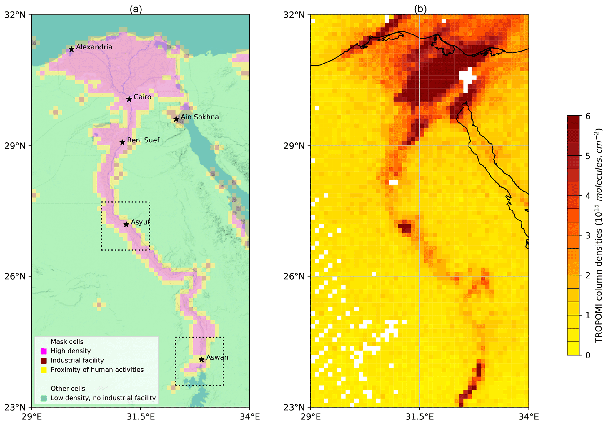
Figure 1(a) Part of Egypt centred on Nile River. Within this domain, pink cells represent locations with an average human density above 100 inhabitants per square kilometre, brown cells represent locations with industrial facilities outside cities and yellow cells represent locations in their vicinity. These cells constitute the mask used to calculate anthropogenic emissions. Outside this mask, green cells represent areas which do not correspond to any of the three criteria, considered to be void of human activity. Five large cities in the country and the industrial area of Ain Sokhna are denoted with stars. Two smaller domains centred around the cities of Asyut and Aswan are represented with dotted lines; their use is presented in Sect. 4.6. (b) TROPOMI observation of NO2 slant column densities above Nile valley on 3 January 2019. White pixels correspond to areas with low-quality data (qa<0.75) or no data.
With an atmospheric lifetime of about a few hours, the presence of NO2 is relatively short. Consequently, the majority of NO2 is not transported far downwind from its sources. Thus, near-surface NO2 concentrations are generally high over industrial facilities and densely populated areas that need to be identified. Because Egypt's population is almost entirely located along the Nile River and its delta, the study of NOx emissions in this country cannot therefore be reduced to the study of a small number of point sources, as would be the case for several other parts of the Middle East region, and must be carried out in the form of a mapping of the country. Further discussion is provided in Sect. 3.3. To identify urban areas in Egypt, we use the Socioeconomic Data and Applications Center (SEDAC) GRUMP (Global Rural-Urban Mapping Project) data archive, which comprises eight global datasets, including a population density grid provided at a resolution of 30 arcsec, with population estimates normalised for the year 2000 (CIESIN, 2019). We combine this database with field data giving the location of industrial facilities from energy-intensive industries in the region. Data have been retrieved from the Global Energy Observatory for five oil- and gas-fired power plants, from the work of Elvidge et al. (2016) for flaring sites, and from the work of Steven J. Davis and Dan Tong (unpublished data) for cement plants; links are at the end of this article. The locations of other industrial facilities, such as aluminium and iron smelters, were obtained from various sources.
These datasets are used to remove the non-anthropogenic part of the NOx emissions signal. We conduct this removal by subtracting the mean emissions over areas without human activity from the mean emissions over industrial and densely populated areas. In order to perform this distinction between these two types of areas, our study is carried out using a mask within a grid. A grid cell is considered to be part of the mask if it has a population density higher than a threshold of 100 inhabitants per square kilometre, or if its centre is close to an industrial facility. Otherwise, the cell is considered to be part of the “background”, i.e. outside the mask. In order to avoid any smearing that would correspond to abnormally high emissions outside urban and industrial centres (which can happen if the wind is poorly estimated), transition cells (in the immediate vicinity of the mentioned mask cells) are also considered to be mask cells. Figure 1 shows the distinction between mask cells and background cells on our domain in Egypt that lies between parallels 23 and 32∘ N and meridians 29 and 34∘ E. Most of the mask cells are located in the Nile area. Some mask cells are also found on the coast or in isolated parts in the desert. They correspond to remote industrial facilities, including major flaring sites, or sparsely populated industrial centres such as Ain Sokhna's industrial area. The domain comprises nm=949 mask cells and nb=3692 background cells. The mathematical description of the background removal is outlined in Sect. 3.4.
2.5 Emission inventories
We compare TROPOMI-derived NOx emissions to the Emissions Database for Global Atmospheric Research (EDGARv5.0) for 2020 and the CAMS global anthropogenic emissions (CAMS-GLOB-ANT_v4.2) inventory released in 2020. Both datasets provide gridded emissions for different sectors on a monthly basis. EDGARv5.0 emissions are based on activity data (population, energy production, fossil fuel extraction, industrial processes, agricultural statistics, etc.) derived from the International Energy Agency (IEA) and the Food and Agriculture Organization (FAO), corresponding emission factors, national and regional information on technology mix data, and end-of-pipe measurements. The inventory covers the years 1970–2015 and differs from the previous version EDGARv4.3.2, which does not use splitting factors derived from the Energy Information Administration (EIA) data on fuel consumption of coal, oil and natural gas for specific countries (Crippa et al., 2020). CAMS-GLOB-ANT_v4.2 is developed within the framework of the Copernicus Atmospheric Monitoring Service (Granier et al., 2019). For this inventory, NOx emissions are based on various existing sectors in the EDGARv4.3.2 emissions from 2000–2012, which are used as a basis for 2010 emissions and are extrapolated to the current year using 2011–2014 sector-based trends from the Community Emissions Data System (CEDS) inventory (Hoesly et al., 2018). From one inventory to another, the names and definitions of the sectors may vary. In EDGARv5.0 and CAMS-GLOB-ANT_v4.2, the emissions for a given country are derived from the type of technologies used, the dependence of emission factors on fuel type, combustion conditions, and activity data and low-resolution emission factors (Janssens-Maenhout et al., 2019).
3.1 Calculation of NO2 production from TROPOMI observations
As a first step, we use tropospheric NO2 vertical column densities to derive top-down NO2 production maps. Vertical column densities are obtained from TROPOMI slant column densities using an air mass factor (AMF) which is also provided by TROPOMI. Previous studies have shown that the use of the AMF is a source of structural uncertainty in NO2 retrievals (Boersma et al., 2004; Lorente et al., 2017). In polluted environments, this source of uncertainty becomes non-negligible. Here, the AMF does not vary much temporally throughout the studied period and is around 1.6 for mask cells and around 1.9 for background cells. The difference between the two types of cells is probably due to a different albedo between the urban environment and desert areas. Using the horizontal wind w, the NO2 flux is given as . The divergence of this flux can be added to the local time derivative to balance NO2 sources and sinks according to the continuity equation
In steady state, the time derivative disappears and the mass balance is reduced to three terms. The NO2 production can thus be estimated by taking the combined effect of atmospheric transport losses and the different sinks. For the transport term, we calculate numerical derivatives with a fourth-order central-finite difference scheme for each cell of the domain. Moreover, since the local overpass time of TROPOMI occurs in the middle of the day, NO2 losses are largely dominated by the three-body reaction involving NO2 and OH (Seinfeld, 1989). Two channels have been identified for this reaction (Burkholder et al., 2020), leading to the production of nitric acid HNO3 and pernitrous acid HOONO:
For the OH concentrations that are considered in this region (1–20×106 molec. cm−3), the reactions above follow first-order kinetics. The total sink term can therefore be calculated as with
τ appears here as the characteristic mixed lifetime of NO2 in the atmosphere. The reaction rate kmean characterises the reactions between NO2 and OH and depends on atmospheric conditions. Burkholder et al. (2020) provide a general expression of this rate as a function of both temperature T and total air concentration [M]. Note that HOONO can be rapidly decomposed back to NO2 and OH in the lower troposphere. We assume here that this decomposition is slow and does not affect the NO2 horizontal gradients. Both pathways are therefore taken into account, and the value of kmean represents the total loss of NO2 due to OH, with a contribution of the HOONO-forming reaction between 5 % and 15 % under atmospheric conditions (Sander et al., 2011; Nault et al., 2016). Thus, the NO2 production can be calculated as the sum of a transport term and a sink term:
The treatment for NOx removal is simplified here. NOx concentrations are influenced by other sinks. Stavrakou et al. (2013) showed that the reaction between NO2 and OH forming HNO3 accounted for most of total NOx loss at the global scale, but with high uncertainties associated with other sinks. Here, the features of the climate in Egypt during daytime hinder many processes to have a significant effect. The following NOx sinks, which can be of notable importance at the global scale, are not taken into account here.
-
NO2 deposition through the leaf stomata of vegetation. This sink can be significant in forested areas. In Egypt, the leaf area index is very low, except in the croplands of the Nile Delta where it is comparable to that of southern Europe or the western United States (Fang et al., 2019), for which the corresponding lifetime was about 10–100 h (Delaria et al., 2020), i.e. about an order of magnitude larger than the lifetimes calculated here. To our knowledge, there are no studies focusing on the corresponding lifetimes for croplands, and we therefore do not take this sink into account.
-
NOx oxidation by organic radicals to produce alkyl and multifunctional nitrates (Sobanski et al., 2017). This sink increases with the concentration of volatile organic compounds (VOCs), whose presence cannot be excluded in Egypt. Different models have estimated low biogenic isoprene emissions in the region (Wiedinmyer et al., 2006; Guenther et al., 2006). These emissions are concentrated around the Nile River and its delta and do not exceed 15 mg m−2 d−1. They are certainly noticeable and higher in summer than in winter, and contrast with the rest of the country, but they remain low compared to other regions in the world. They are, for instance, about an order of magnitude lower than in the forested areas of the eastern US, where the corresponding sink accounts for between 30 % and 60 % of the total NOx sink (Romer Present et al., 2020). Furthermore, at large NO2 concentrations (compared to VOC concentrations), the share of this sink in the total NOx loss is weakened compared to that of HNO3 (Romer Present et al., 2020). The effect of biogenic emissions of VOC can therefore be considered minor. However, VOC emissions can also be of anthropogenic origin, especially in urban areas, where they are difficult to estimate. To our knowledge, there is no study evaluating the competition of the two sinks in Egypt or in a region with similar features, and we therefore do not account for this reaction in our calculations.
-
NO reaction with HO2 to produce nitric acid (Butkovskaya et al., 2005), whose yield is strongly enhanced in presence of water vapour (Butkovskaya et al., 2009). Here, we neglect this reaction as the corresponding reaction rate is lower by a factor of 3 to 8 in dry conditions (Butkovskaya et al., 2005).
-
NO conversion to NO3, the latter being in thermal equilibrium with NO2 and N2O5. This sink, which takes place via heterogeneous processes, has a significant contribution during nighttime in the Mediterranean region (Friedrich et al., 2021) and is neglected at 13:30 LT when OH is close to its daily maximum.
-
NO2 reversible reaction with peroxyacetyl radical to produce peroxyacetylnitrate (Moxim et al., 1996). In the Nile Delta region, PAN concentrations in the lower troposphere are significantly below the global average (Fischer et al., 2014), possibly due to high temperatures favouring short PAN lifetimes. Moreover, its production peaks in the late afternoon and early evening (Seinfeld, 1989). We therefore do not consider this sink in the representation of NOx emissions at 13:30 LT.
-
NO2 uptake onto black carbon particles (Longfellow et al., 1999). This uptake is of a limited amount in the Mediterranean region (Friedrich et al., 2021).
With all these processes not being accounted for, the reaction between NO2 and OH is the only sink that is considered in our calculations to provide an indication of NOx emissions. Section 4.7 details the consequences of not considering these various minor sinks on the results.
3.2 Interpolation to daily average emissions
All parameters are evaluated at 13:30 LT, which means that the NO2 production is calculated at the same moment. In Egypt, the maximum and minimum electricity consumption is reached around 20:00 and 06:00 LT respectively, and inter-daily consumption differences have been weakened by the increasing sales of air conditioning and ventilation systems in the past decades (Attia et al., 2012). The daily load profiles provided by the National Egyptian Electricity Holding Company show that the mean daily electricity consumption corresponds approximately to the consumption at 13:30 LT in the country (EEHC, 2021). The difference between the two quantities being small both in summer (about +2 % to −3 %) and winter (about −2 % to −6 %), we consider our inferred emissions to be representative of the average activity in Egypt at any time of the year. This assumes that electricity consumption dominates the emissions of the country, or that the other emitting sectors have a similar daily profile. This can be justified. According to CAMS-GLOB-ANT_v4.2, the power sector accounts for 50 % to 60 % of total NOx emissions in Egypt. EDGARv5.0 presents a lower share (40 % to 45 % of total emissions). Moreover, for both inventories, the transport sector accounts for the majority of the remaining emissions. According to the traffic congestion index in Cairo (https://www.tomtom.com/en_gb/traffic-index/cairo-traffic/, last access: 21 April 2021), the congestion level around 13:30 LT seems to be slightly higher than during the morning peak, but lower than during the night peak. Traffic emissions at this moment of the day could therefore be representative of the average traffic emissions as well.
3.3 Validation of CAMS OH concentration using line density calculations for Riyadh
When the transport term is integrated over large spatial scales, it cancels out due to the mass balance in the continuity equation between NO2 sources and NO2 sinks. At first order, the integration of the inferred emissions over the whole domain (of about 490 000 km2) thus reflects chemical losses of the sink term. In this term, the NO2 lifetime calculation involves the reaction rate kmean, whose annual variability is low due to small changes in Egyptian midday temperatures throughout the year, and OH concentration, whose annual variability is highly marked. In Egypt, tropospheric OH concentrations, which are strongly correlated with solar ultraviolet radiation (Rohrer and Berresheim, 2006) and NOx emissions, are higher in summer than in winter. To ensure an appropriate representation of the OH field by CAMS data, we select a large number of TROPOMI images characterised by a homogeneous wind field, in which we calculate the NO2 lifetime according to Eq. (2), where [OH] corresponds to the near-real-time CAMS data and kmean is calculated with the formula from Burkholder et al. (2020). We compare this value with the lifetime determined by a method initially developed by Beirle et al. (2011), and expanded by Valin et al. (2013) by introducing a rotation of the image to refine the chemical lifetime. This method consists in fitting an exponentially modified Gaussian function (EMG) to NO2 line density profiles. These profiles correspond to the integrated NO2 columns along the mean wind direction in the pollution pattern and centred around the source. They are obtained by rotating TROPOMI images in the mean wind direction and using the values of the nearest columns in a 100 km2 area. Line density profiles are generated on a span of 300 km. An example is given in Fig. 3. Within the average profile, the NO2 burden and lifetime can be derived from the parameters that describe the best statistical fit. The EMG model is expressed as follows (Lange et al., 2022):
Here, x is the distance in the downwind–upwind direction; B is the NO2 background; A is the total number of NO2 molecules observed in the vicinity of the point source; x0 is the e-folding distance downwind, representing the exponential length scale of NO2 decay; μ is the location of the apparent source relative to the centre of the point source; and σ is the standard deviation of the Gaussian function, representing the length scale of Gaussian smoothing. Using a non-linear least-squares fit, we estimate the five unknown parameters: A, B, x0, μ and σ. From the mean wind module wmean in the domain, the mean effective NO2 lifetime τfit can be estimated using the fitted parameters:
The geography of Egypt does not suit the method described here. The Egyptian population is contiguously concentrated along the Nile, which makes it difficult to define point sources isolated from human activity. Furthermore, large isolated cities such as Alexandria or Suez are too close to the coast for the wind to be considered homogeneous. We therefore use the city of Riyadh, Saudi Arabia (24.684∘ N, 46.720∘ E), to perform the comparison between the CAMS-induced lifetime and the fit-obtained lifetime. Riyadh has been the focus of anterior studies (Valin et al., 2013; Beirle et al., 2019) and is particularly suitable for several reasons. Firstly, Riyadh is a city within the latitudinal extent of Egypt (1600 km from Cairo) with a climate that is similar to the typical Egyptian climate. Secondly, NO2 tropospheric columns over Riyadh are high ( molec. cm−2), leading to retrievals with a high signal-to-noise ratio. Thirdly, Riyadh is far from the coast, and its flat terrain makes the surrounding wind fields rather homogeneous during most of the year.
As the fitting algorithm is very sensitive to any disturbance that might be induced by NO2 production from other point sources, it is necessary to identify heavy industrial facilities in the area. Riyadh is also an industrial area, with several power plants located close to the city centre. Figure 2 shows the location of the most important emitters in the region, which include five gas-fired power plants (PP7, PP8, PP9, PP10 and PP14), one oil-fired power plant (PP4) and one cement plant (CP). The five gas power plants, with a total capacity of more than 10 GW, are located in the periphery of the city. These power plants are sufficiently far away from the city centre for TROPOMI to distinguish their own emissions from those of Riyadh’s centre with a resolution of , which is not the case for CP and PP4, which are located in the city centre. It is therefore appropriate to restrict the study of NO2 patterns over Riyadh to days for which the emissions from the city centre and those from the gas power plants do not overlap. This is the case when the wind blows steadily and homogeneously in a north–south direction. Within about 150 km around the city centre, we thus calculate the average wind given by ERA5 and consider the observation to be reliable if the mean angle 〈θ〉 of the observations deviates by less than 40∘ from the north or the south, with a standard deviation σθ of less than 36∘. This condition generally leads to a selection of observations with large wind speeds, low winds speeds being often associated with more variable directions. This ensures the NO2 decay to be dominated by chemical removal and not by the variability of the wind (Valin et al., 2013). Finally, we select observations with clear-sky conditions downstream of the flow (with at least 80 % downstream cells with qa>0.75).
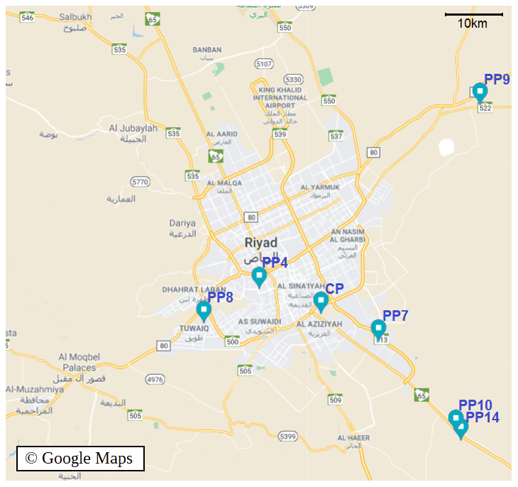
Figure 2Map of Riyadh's city centre with the surrounding power plants (PP4, 7, 8, 9, 10 and 14) and cement plant (CP). The map has been extracted from © Google Maps.
Our gridding ensures that retrieved lifetimes are governed by physical decay of NO2 and not an artefact of the spatial resolution (Valin et al., 2011). The fitting procedure is very sensitive to the wind direction. Instead of manually correcting the ERA5 wind field for individual NO2 patterns, the curve fitting is performed for every sample with three different rotation angles, corresponding to the wind direction with a correction of −10, 0 or 10∘. A record is kept if one of these three fits leads to a correlation with the corresponding NO2 line density whose coefficient is greater than 0.97. Among the remaining samples, we keep those with a value of τfit greater than 1.0 h (considered sufficiently high to be relevant). An example of curve fitting is given in Fig. 3.

Figure 3Estimation of the NO2 lifetime from a pattern above Riyadh on 11 March 2020: (a) NO2 plume rotated with its wind direction around the source (star) to an upwind–downwind pattern. Grey boxes centred around black points indicate the extent of the spatial integration of NO2 columns to obtain the NO2 line density. Values of cardinal points are noted in black. (b) Corresponding line densities (points) representing the downwind evolution of NO2 as a function of the distance to Riyadh's city centre and the corresponding fit according to the exponentially modified Gaussian function (dashed line).
The phenomena under study here take place in the planetary boundary layer (PBL), which in this region has a midday height of about 2 km (Filioglou et al., 2020). TROPOMI observations only provide information on the total NO2 content of the tropospheric column, without providing information on the vertical distribution of concentrations. Extracting emissions from concentrations therefore requires a selection on the height at which wind, temperature and OH data are taken. Lama et al. (2020) and Lorente et al. (2019) conducted similar studies using the boundary layer average wind, while Beirle et al. (2019) chose a vertical level of about 450 m above ground. Because vertical transport of NOx, which is emitted mainly from combustion engines and industrial stacks, is generally minor compared to horizontal transport, NOx is confined to the first few hundred metres above ground level. Using PBL-averaged data poses a problem of consistency as wind, temperature and OH concentration values significantly vary within the PBL. As a consequence, we compare the CAMS-induced lifetime τ and the fit-induced lifetime τfit using the parameters (w, [OH] and T) at two different vertical levels: a medium level 𝒜 at 925 hPa (about 770 m a.g.l. – above ground level) and a bottom level ℬ at 987.5 hPa (about 210 m). These levels are interpolated from four and two ECMWF or CAMS consecutive pressure levels respectively (1000–850 hPa for level 𝒜 and 1000–975 hPa for level ℬ). Since most mask cells have an altitude between 0 and 150 m, the corresponding pressure variations are small (up to ∼16 hPa), which allows us to neglect the effects of topography on the position of pressure levels. Figure 4 sums up the selection method for the comparison of lifetimes.
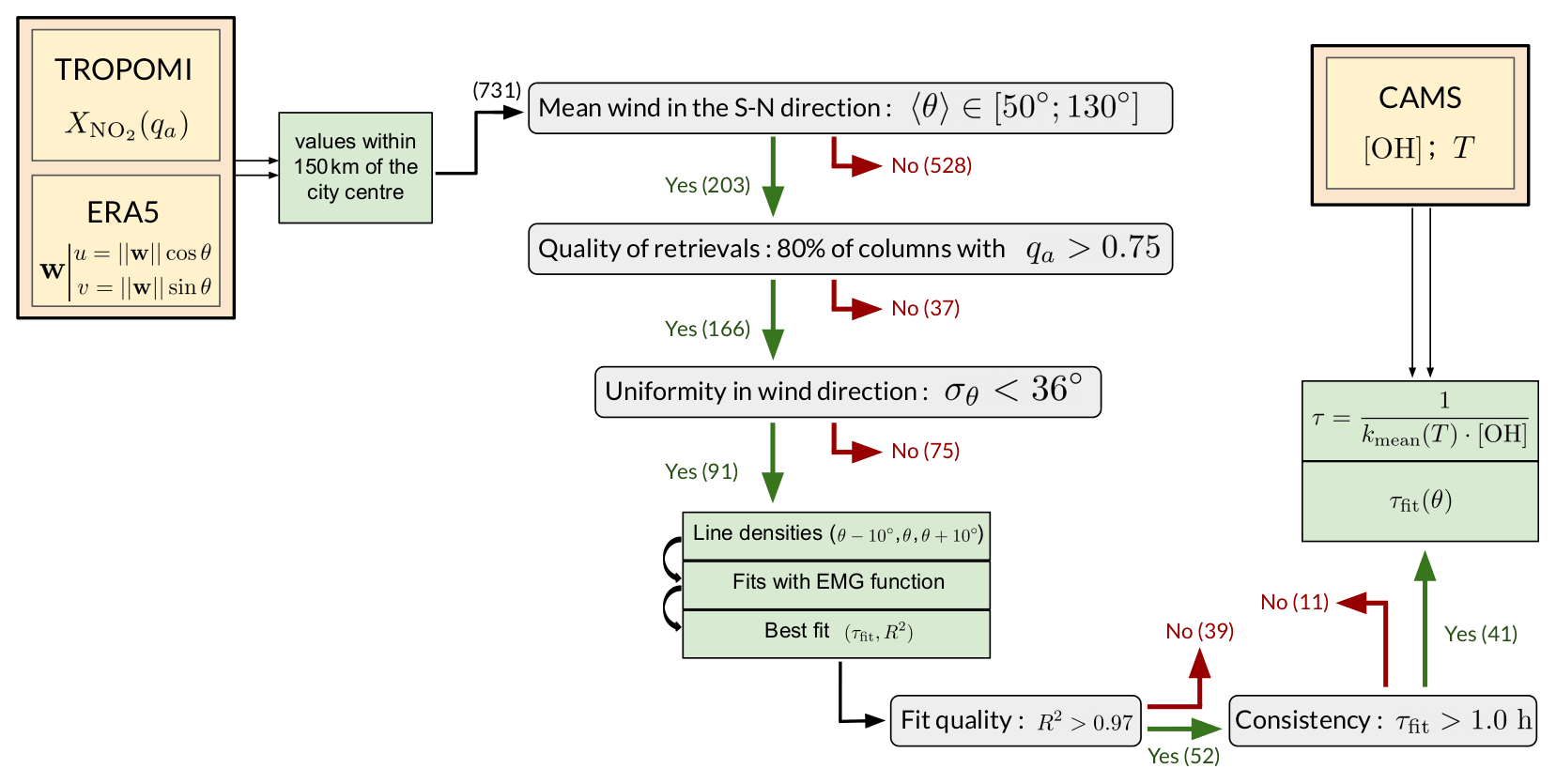
Figure 4Selection method for NO2 patterns over Riyadh. Datasets (yellow-orange) are used to calculate the quantities (light green) that are submitted to different tests (grey). A total of 731 patterns are progressively conserved (green arrows) or rejected (red arrows). At each stage, the number of conserved or rejected patterns are noted within brackets (the value is only given for calculations performed at level ℬ). This selection process compares the lifetimes estimated by the EMG function fitting with TROPOMI line density profiles to the lifetimes calculated according to Eq. (2) with CAMS data.
3.4 Calculation of anthropogenic NOx emissions and comparison with inventories
We calculate NOx emissions on the entire domain from NO2 production by using CAMS NO and NO2 concentrations. These are not intended to replace TROPOMI observations; they are used to apply the concentration ratio to account for the conversion of NO2 to NO and vice versa. As diurnal NO concentrations in urban areas generally range from 10 to 150 ppb (Khoder, 2009), the characteristic stabilisation time of this ratio never exceeds a few minutes (Graedel et al., 1976; Seinfeld and Pandis, 2006). Since this time is lower than the order of magnitude of the inter-mesh transport time (about 30 min considering the resolution used and the mean wind module in the region), we can reasonably neglect the effect of the stabilisation time of the conversion factor on the total composition of the emissions and treat each cell of the grid independently from its neighbours. Beirle et al. (2019) found an annual average of 1.32 for this conversion factor, but CAMS data show small deviations from this value over Egyptian urban areas. We therefore calculate NOx emissions for each cell of the domain as follows:
For convenience, quantities and represent the respective contributions of the transport and the sink terms to total NOx emissions. We finally obtain the emissions related to human activity by removing the arithmetic mean value of NOx emissions above background cells from total emissions:
These removed emissions are linked to the NO2 background estimated by TROPOMI. This background, which is mostly located in the upper troposphere, is inconsistent with the use of other parameters which are calculated in the lower troposphere. As such, these emissions do not correspond to anthropogenic emissions, but they provide the value of what must be subtracted from the estimates to obtain emissions related to human activity. Such a removal assumes that other processes involved in NOx budgets lead to similar emissions inside and outside the mask, which is not evident, as the majority of background cells are located in the desert or the ocean while the majority of mask cells are located near the Nile River. However, as the processes involved in natural NOx sources lead to emissions much smaller than anthropogenic emissions in polluted areas, we neglect this difference in the following calculations. An alternative would be to calculate an average concentration for the background cells and subtract the corresponding value from the column densities before calculating the emissions. This would pose further reliability problems: for instance, very high NO2 concentrations could appear outside the mask due to wind transport (an example is shown in Fig. 1). They would lead to an overestimation of the NO2 background and thus to an underestimation of the anthropogenic emissions.
Neglecting the part of the country that lies outside the domain, total emissions from the anthropogenic activity of Egypt can then be obtained by integrating on the whole domain. For robust statistics, these derived emissions can be averaged monthly, enabling a month-by-month comparison with bottom-up inventories. The linearity of the averaging processes ensures the interchangeability of temporal and spatial averages. A monthly average is relevant because it aggregates enough data to limit the impact of the outliers due to uncertainties in wind and OH representation. In addition, it enables the study of monthly NOx emission profiles, which reflect changes in human activities throughout the year due to temperature changes, economic constraints and cultural norms.
4.1 Line densities and NO2 lifetime
We compare the results of the TROPOMI line density fits for Riyadh to the lifetime calculated by Eq. (2) using CAMS OH data. The 2 years of TROPOMI observations (from November 2018 to November 2020) provide a wide variety of profiles. For level ℬ, Fig. 4 also provides the number of samples that are being kept at each stage of the process. Of the 731 observations available, 203 have a wind direction in the cone with a north–south orientation with an aperture of 40∘ (i.e. between 340 and 20∘ or between 160 and 200∘). Of the remaining observations, 166 occurred with a sufficiently clear sky to be retained. The criterion of weak variability for the wind direction brings to 91 the number of observations that are kept by the method. With these 91 observations, the line density profiles are calculated and the fits applied. According to Eq. (5), the lifetime is calculated using the mean wind module around the point source. The two lifetimes are calculated with the parameters taken at the medium level 𝒜 or at the top level ℬ. Of the 91 fits obtained, 51 are of high quality (correlation coefficient between fit function and line density profile greater than 0.97) for level 𝒜 and 52 for level ℬ. A total of 39 of these fits lead to a lifetime τfit greater than 1.0 h for level 𝒜 and 41 for level ℬ. All remaining samples correspond to atmospheric conditions with moderate to fast winds, with a module ranging between 2 and 11 m s−1 (with an average of 5.9 m s−1) for level 𝒜 and between 3 and 8 m s−1 (with an average of 5.4 m s−1) for level ℬ. These lifetimes are compared to the corresponding lifetimes obtained from CAMS data in Fig. 5, which is divided into seasons for a more convenient comparison. The use of level 𝒜 leads to notable underestimations of the NO2 lifetime in autumn compared to the lifetime calculated with the fitting method. This same level leads to lifetime overestimations in winter. This trend is not found with the use of level ℬ, which leads to a better reproduction of the lifetimes calculated with the fitting method for the available seasons. Figure 5 shows a linear regression between the two calculated lifetimes. The results are scattered, with a correlation coefficient higher for level ℬ (0.408) than for level 𝒜 (0.220). When the intercept of the regression line is forced to zero, the resulting slope is closer to 1 for level ℬ (0.998) than for level 𝒜 (1.071).
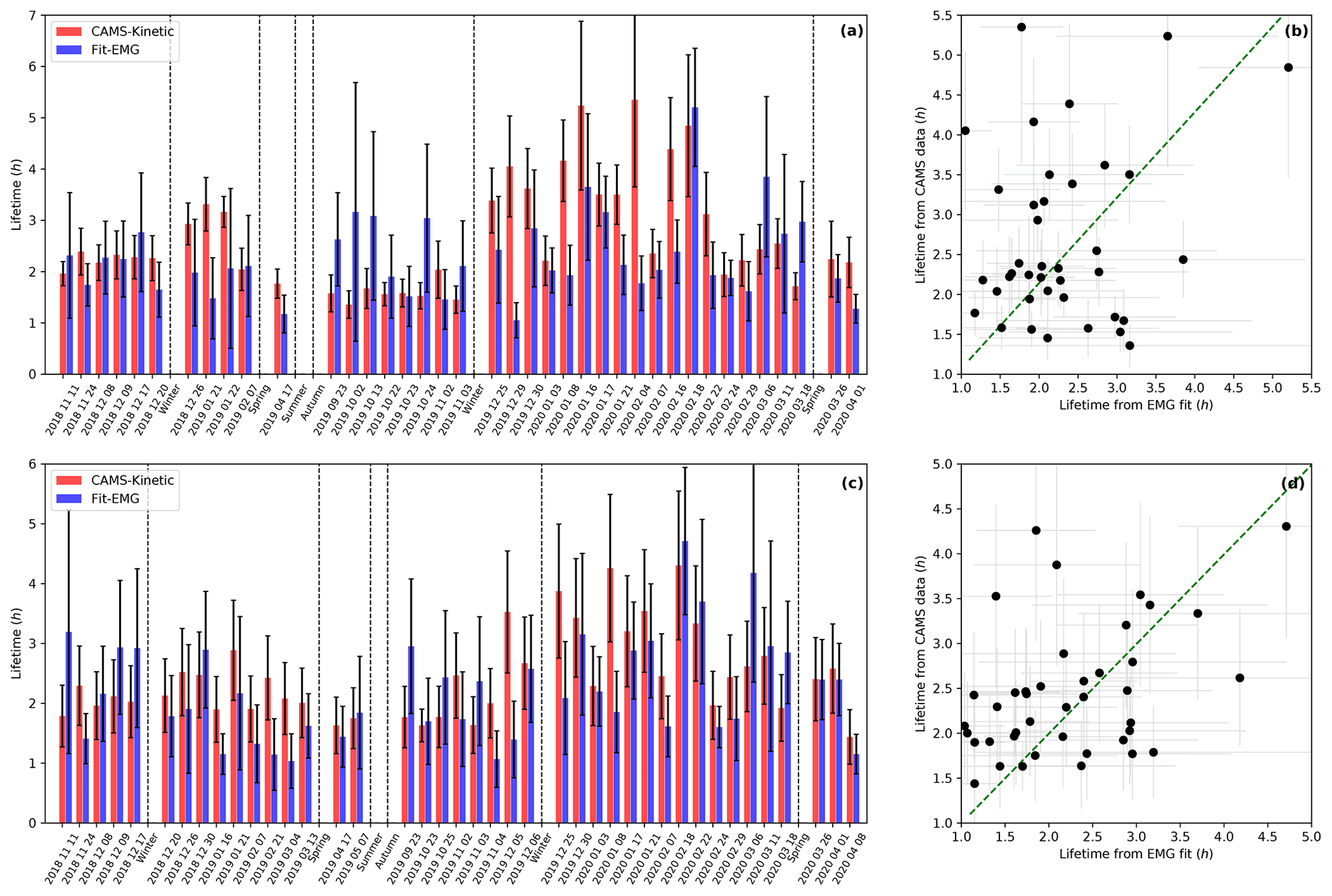
Figure 5(a, c) Comparison between CAMS-derived NO2 lifetimes and lifetimes from NO2 line density fittings with EMG function above Riyadh city centre, for levels 𝒜 (a) and ℬ (c). The samples presented correspond to patterns in clear-sky conditions for which the mean wind is in the north–south direction with a low variance, and for which the correlation between line density profile and fit gives a correlation coefficient of more than 0.97 and a lifetime of more than 1.0 h. NO2 patterns do not have these conditions during the summers of 2019 and 2020. Dashed lines separate the groups of observations by season. (b, d) Comparison between the two calculated lifetimes for levels 𝒜 (b) and ℬ (d). A linear regression with an intercept forced to be zero is displayed with a green dashed line.
Although both correlations are weak, level ℬ leads to a better match between the lifetime calculated with Eq. (2) and the lifetime calculated from line densities. The results that are presented in the following sections (except for Sect. 4.3) are therefore results of calculations performed with parameters (w, [OH], T and ) estimated at level ℬ. Nevertheless, it should be noted that no summer observations were included in the comparison. The main reason for this is the wind direction: of the 188 summer days observed, 178 have a mean wind direction outside the north–south cone over central Riyadh. On the remaining 10 d (one for summer 2019 and nine for summer 2020), the ERA5 wind direction is too variable for the fit to be considered relevant, or the fit results in a correlation coefficient below 0.97. It is not clear how correctly the NO2 lifetime would be calculated during both summer periods by Eq. (2). With OH concentrations being the main driver of this lifetime, we cannot assess the relevance of the representation of OH concentrations by CAMS data during summer days in the study.
4.2 Mapping of Egypt's NOx emissions
As a first step, we try to map NOx emissions in Riyadh using parameters estimated at level ℬ. For the period from December 2017 to October 2018 and using a constant lifetime of 4 h, Beirle et al. (2019) estimated at 6.66 kg s−1 the emissions of the corresponding urban area and a mean rate density of about 3.7 µg m−2 s−1 for power plants PP9 and PP10–14, with the transport term accounting for about 80 % to 90 % of this budget. Using the same domain for December 2018 to October 2019 with our method, we found a mean lifetime of 2.94 h and mean emissions of 5.92 kg s−1 for the urban area. We also found smaller rate densities for the power plants (about 3.4 µg m−2 s−1 for PP9 and 3.0 µg m−2 s−1 for PP10–14), with a smaller contribution of the transport term (about 70 %). Despite differences in resolution, AMF calculation, lifetime variability and background removal, the two methods give similar results.
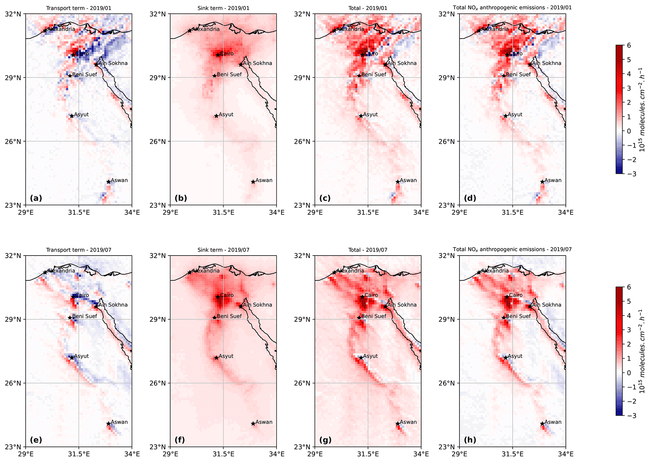
Figure 6NOx emissions above most of Egypt's territory: (a–d) transport term (a), sink term (b), resulting emissions (c) and the corresponding anthropogenic emissions after non-anthropogenic background removal (d) for January 2019. (e–h) Transport term (e), sink term (f), resulting emissions (g) and the corresponding anthropogenic emissions after background removal (h) for July 2019.
The top-down emission model is then applied to the Egyptian domain with CAMS OH concentration and temperature fields for lifetime calculations. For each cell, NOx emissions are calculated according to Eq. (6), resulting in a mapping of Egypt's emissions. The obtained values are averaged monthly from November 2018 to November 2020. Figure 6 shows a composition of the emissions map with the transport term and the sink term for the months of January and July 2019. The corresponding anthropogenic emissions, calculated according to Eq. (7), are added. The Nile appears on transport term maps: the divergence calculation complies with what is expected from a line of emitters, i.e. a clear separation of zones of positive divergence from zones of negative divergence with a separation line corresponding to the course of the river. The fact that areas of negative and positive divergence are respectively located to the east and the west of the river is the result of the zonal component of the wind being positive most of the time. Some point sources like Cairo, Alexandria, Asyut or Aswan are easily identifiable. The sink term, directly proportional to the TROPOMI column densities, also highlights these cities. However, unlike the transport term, which has a similar spatial pattern from month to month, the sink term is clearly stronger in summer than in winter. This is mainly due to a higher lifetime in winter than in summer (4.94 h on average in January 2019 and 2.62 h in July 2019) while the average TROPOMI NO2 concentrations are slightly higher during winter (1.071×10¹⁵ molec. cm−2 for January 2019 and 0.899×10¹⁵ molec. cm−2 for July 2019). Over the whole domain, the mean transport term varies throughout the studied period between molec. cm−2 h−1 (December 2019) and 0.015×10¹⁵ molec. cm−2 h−1 (May 2020). Thus, it hardly contributes to the NOx emission budget, with the mean chemical sink term alone varying between 0.223×10¹⁵ molec. cm−2 h−1 (December 2019) and 0.534×10¹⁵ molec. cm−2 h−1 (September 2020).
Table 1Comparison between the transport term and the sink term above different cities in Egypt, as well as the industrial region of Ain Sokhna located 45 km southwest of Suez for January and July 2019. TROPOMI vertical NO2 columns, NOx emissions and population densities correspond to average values within 18 km from the city centre. Unit ℳ stands for a quantity of 1015 molecules (NO2 or NOx).
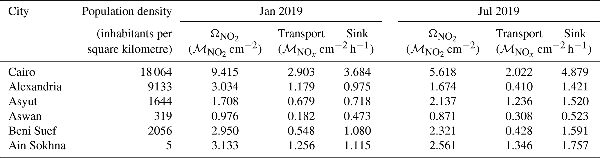
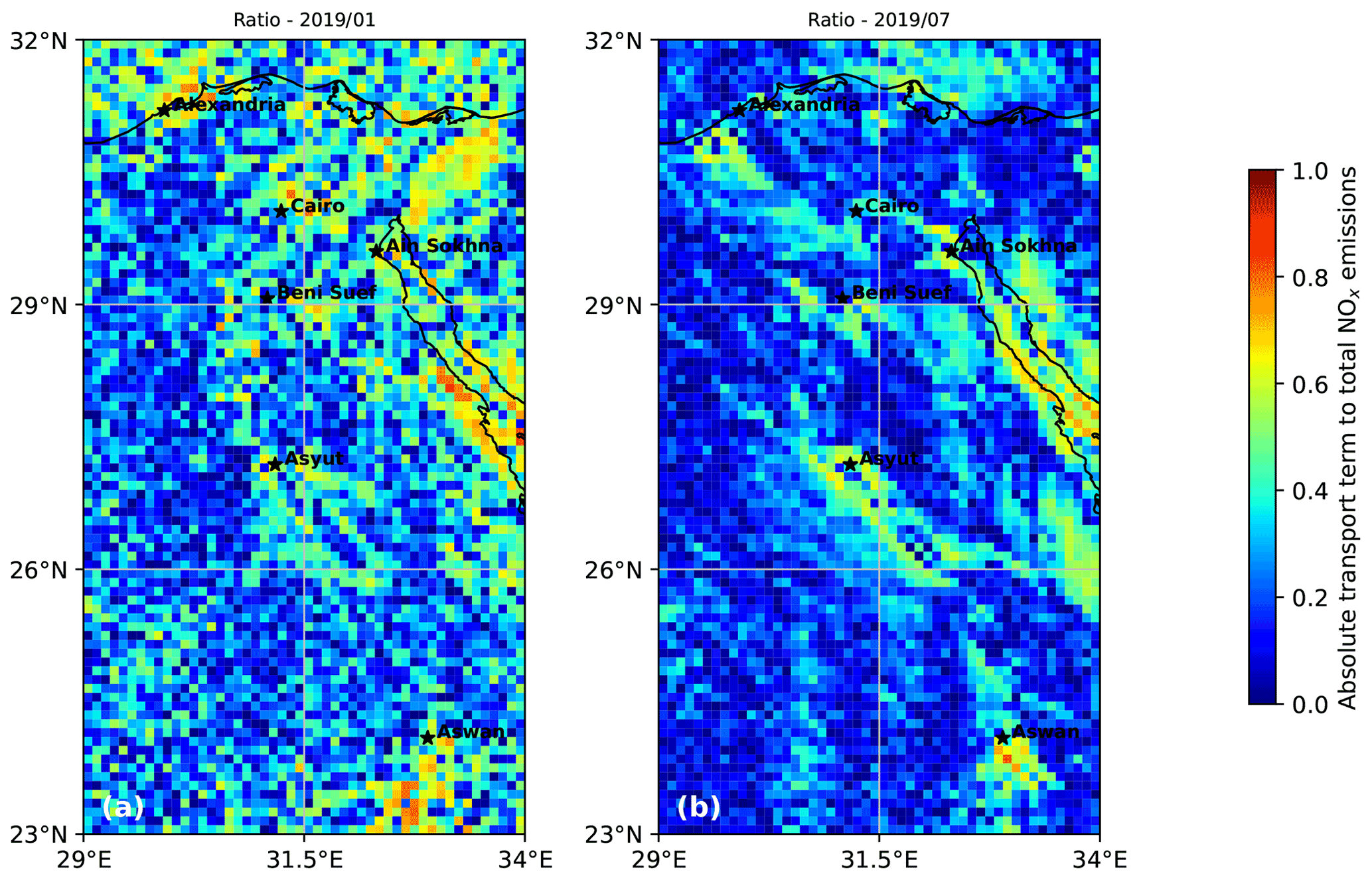
Figure 7Share of the absolute value of the transport term in the sum of the sink term and the absolute value of the transport term above most of Egypt's territory, indicating the local importance of the transport term in NOx emissions above mask cells. The average of this ratio is shown for January 2019 (a) and July 2019 (b).
Several cities in the country appear as the main emitters of the country, such as Cairo, Alexandria, Beni Suef, Asyut or Aswan. The industrial area of Ain Sokhna, located southwest of Suez, also appears as a main emitter. Table 1 compares the monthly values for the sink term and the absolute value of the transport term above five major cities of the country, with populations ranging from 200 000 to 20 million inhabitants, as well as Ain Sokhna's area. The mean values for TROPOMI column densities are also provided. According to the results, the capital city of Cairo is by far the largest emitter in the country, largely due to its large population, resulting in high traffic emissions, but also to its intensive industrial activity. Alexandria, the country's second largest city, is not necessarily the second largest emitter, as its emissions are comparable to those of smaller cities such as Beni Suef or Asyut. However, the three cities concentrate a large amount of industrial activity: Alexandria hosts several oil and gas power plants and a small number of cement factories, while Beni Suef is close to several oil and gas power plants and hosts several flaring sites. Similarly, the city centre of Asyut is close to three oil and gas-fired power plants and a cement factory. This seems to indicate that industrial activity might be the main cause of NOx emissions differences between these cities, before population size. This explains why NOx emissions from these three cities are comparable to those of the industrial area of Ain Sokhna, which includes several cement facilities, iron smelters and oil and gas plants. It might also explain why Aswan, which has a population that is comparable to Beni Suef or Asyut, but which does not have any major industrial site, has slightly lower emissions than the two other cities. An additional analysis of the differences between Asyut and Aswan is provided in Sect. 4.6. Finally, the Gulf of Suez displays relatively large emissions, which might be attributed to the shipping sector, the region being a major gateway for international trade. Because it also hosts several flaring sites, these emissions might also be due to the oil and gas extraction activity.
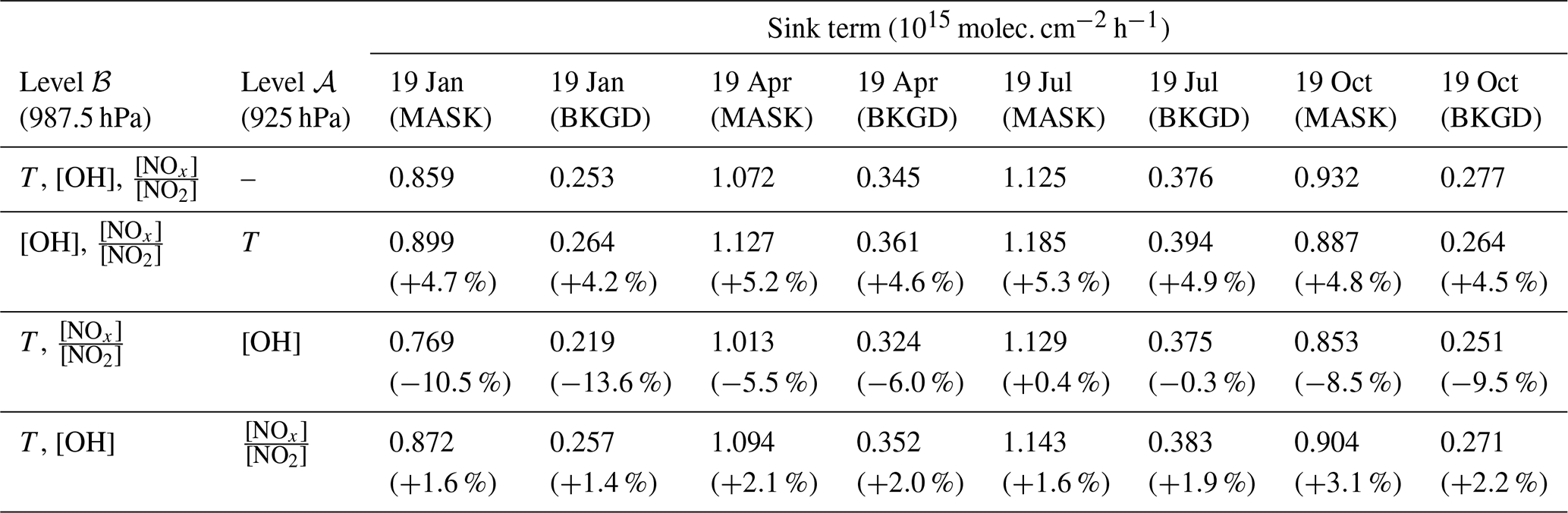
Table 2Analysis of the effect of a vertical change in the parameters used to estimate the mean sink term in NOx emissions: temperature, hydroxyl radical concentration and NOx:NO2 concentration ratio. The comparison is conducted between the estimated quantities at level ℬ and level 𝒜 for mask cells (MASK) and background cells (BKGD) for January, April, October and July 2019. Values within brackets represent the variation from the base case for which all quantities are estimated at level ℬ.
Although these cities and areas can be described as high-emission sites, the terms responsible for these emissions differ from one site to the other. Figure 7 shows the contribution of the transport term (taken in absolute value) to total emissions for January and July 2019. Because wind fields are relatively homogeneous along the Nile on spatial scales of less than 100 km, NO2 concentration gradients perceived by TROPOMI in the region mainly contribute to the increase in the transport term, which can reach similar values as the sink term. However, it is never significantly higher than the sink term: due to a spread of the emissions over large urban areas, the behaviour of these cities is therefore different from that of a point source for which the transport term would be very high (Beirle et al., 2021).
Desert areas such as the Libyan Desert, the Eastern Desert and the Sinai region (located respectively to the west, east and northeast of the Nile) show a very low value for the transport term compared to the sink term, due to the homogeneity of both the wind field and the detected NO2 concentrations in these areas. In the case of the Gulf of Suez, the transport term can be 1 to 2 times higher than the sink term, which varies between 0.4 and 1.2×10¹⁵ molec. cm−2 h−1. Those values are slightly higher than the average emissions above background cells areas due to the sink term (about molec. cm−2 h−1), but remain quite low compared to the emissions in large cities. This relative predominance of the transport term is explained by a visible gradient of the TROPOMI NO2 column densities. The region thus acts as a very thin line of emitters. Nevertheless, this predominance might also be partly due to a poor representation of the wind field. The low resolution of ERA5 (about 26 km in this region, which is the same order of magnitude as the width of the channel) may misrepresent the wind near the coast, creating artificial gradients.
4.3 Vertical analysis
Here we investigate the influence of the choice of the vertical level in the representation of the different model parameters. This influence is of considerable importance, as NOx sources in urban areas can be located at different altitudes. For instance, emissions from the road sector from tailpipes are located at ground level, whereas NOx from power plants and industrial facilities can be emitted from stacks, which are usually located between 50 and 300 m a.g.l. (above ground level). Section 4.1 results showed that level ℬ was more appropriate for the representation of the NO2 lifetime. This level is therefore chosen as a reference for the comparison. We study the effect of a transition from level ℬ to level 𝒜 for each of the three parameters involved in the representation of the sink term, i.e. temperature T, hydroxyl radical concentration [OH] and concentration ratio . The results for the averages over mask cells and background cells are given for the months of January, April, July and October 2019 in Table 2. As the wind field is only involved in the transport term whose spatial integration nearly leads to zero, the influence of this parameter is not studied.
The transition to level 𝒜 generally results in a decrease in temperature, leading to an increase in the reaction rate kmean and thus an increase in the emissions from the sink term. This transition has only a small influence on the total NOx emission estimates, with mask and background cell emissions increasing by 4 % to 6 %. The influence of OH goes in the opposite direction: its concentration decreases with altitude, weakening the sink term. This weakening is particularly visible during winter months, for which the emissions are lower by up to 14 %. In summer however, the effect is hardly noticeable. Finally, the influence of the NOx:NO2 ratio is negligible on the NOx emission estimates. Thus, the transition to level 𝒜 results in an increase in the sink term of 1 % to 4 %, due to a decrease in concentrations of both NO and NO2 with respect to the vertical but with a greater decrease for NO2. This vertical study confirms the crucial importance of the OH concentration for the accurate representation of NOx emissions. It appears here as an important driver of the sink term, which is much more sensitive to vertical differences than temperature or the NOx:NO2 concentration ratio.
4.4 Weekly cycle
In Egypt, the official rest day is Friday, and the economic activity of the country is a priori lower during this day than during the other days of the week. We therefore try to characterise this feature, by evaluating the weekly cycle of NOx emissions. We use the TROPOMI-inferred emissions to obtain averages per day of the week. We use the quality assurance qa of TROPOMI retrievals to ignore the days for which more than 20% of the domain has low-quality data (this happens 43 times in 2018/19 and 28 times in 2019/20). Such a filtering avoids accounting for the days when a large part of the urban and industrial areas is covered by clouds. However, it misses situations where small clouds are localised over large emitters, in which case the corresponding emissions are under-estimated. Figure 8 shows the resulting daily emissions for the period November 2018–November 2019 and November 2019–November 2020. NOx emissions are expressed as NO and in kilotons per day. A Friday minimum is observed, defining a weekly cycle. This trend is also observed for mean NO2 column densities, for which no intra-weekly variation is observed. Over the 2018–2019 period, Fridays have average emissions of 0.811±0.408 kt, which is lower than average emissions for the rest of the week, which reach 0.997±0.533 kt. A similar trend is observed in 2019–2020, for which the average for Fridays is 0.704±0.357 kt and the average for other days is 0.921±0.449 kt. The difference in emissions between the two periods is due to smaller emissions in December 2019, January 2020 and February 2020 that are discussed in Sect. 4.5. On average, Friday emissions correspond to a ratio of 0.83:7 (i.e. a value of 0.83 after normalisation on the seven days of the week) for the entire domain. This result is consistent with the values obtained by Stavrakou et al. (2020), who used TROPOMI data and another emission model to calculate a ratio of 0.71:7 for Cairo and 0.89:7 for Alexandria in 2017.
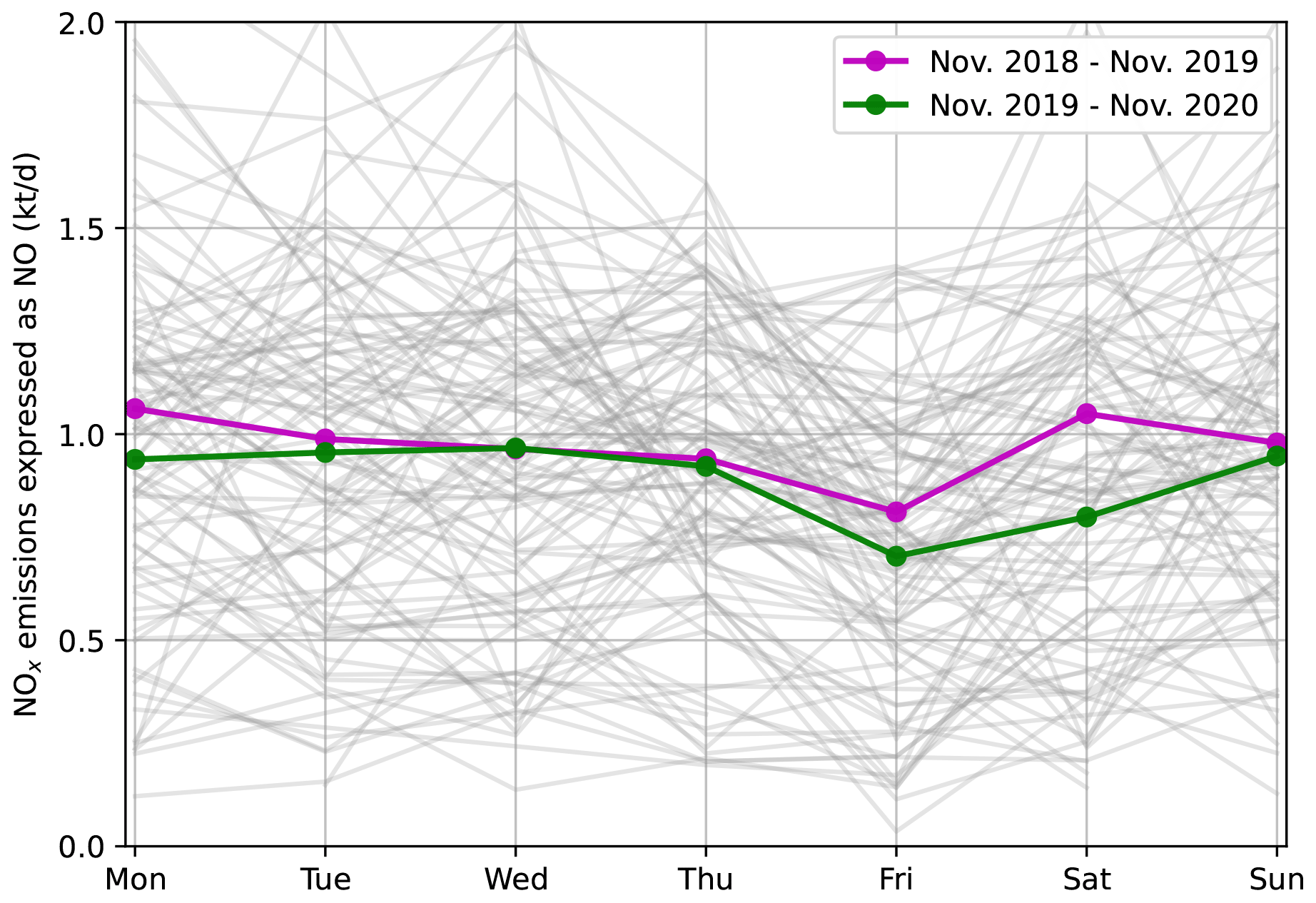
Figure 8Weekly profiles of anthropogenic NOx emissions for Egypt using TROPOMI observations in 2018–2019 (purple line) and 2019–2020 (green line). Thin grey lines represent individual weeks. Days for which less than 80 % of the domain counts low-quality observations (qa<0.75) are not represented.
4.5 Impacts of lockdown during COVID-19
The ongoing global outbreak of COVID-19 forced many countries around the world to implement unprecedented public health responses, including travel restrictions, quarantines, curfews and lockdowns. Such measures have helped to counter the spread of the virus and have, meanwhile, caused high reductions in global demand for fossil fuels (IEA, 2020). They also led to a fall in the levels of NO2 and other air pollutants across the globe (Venter et al., 2020; Bauwens et al., 2020; Gkatzelis et al., 2021). To prevent the spread of COVID-19, Egyptian authorities ordered a partial lockdown from 15 March till 30 June 2020, closing all public areas (e.g. sport centres, nightclubs, restaurants and cafes) and suspending religious activities in all mosques and churches throughout the country. They also implemented more drastic measures such as a full lockdown during Easter (20 April) and Eid (23 to 25 May), before lifting some restrictions on 1 June (Hale et al., 2021). In addition to the effect of containment on the activity of the country, the global decline in consumption led to a drop in the production of certain industrial products.
Several studies have estimated the impact of these events on the air pollution levels in the urban centres of the country: from in situ measurements, El-Sheekh and Hassan (2021) estimated that NO2 concentrations had dropped by 25.9 % in Alexandria’s city centre after the start of the lockdown on 13 March, while Abou El-Magd and Zanaty (2020) used OMI retrievals to estimate a 45.5 % reduction of NO2 concentrations for the entire country during the spring compared to 2018 and 2019 average values. However, due to a changing lifetime of NO2, reductions in the concentrations of NO2 might not be entirely due to a decrease in NOx emissions, which leads us to focus on the variation in NOx emissions during this singular period. Using our top-down emission model, reductions in total NOx emissions of 20.1 %, 11.8 % and 13.5 % are observed for the months of March, April and May 2020 compared to the equivalent months in 2019. This drop of emissions in 2020 compared to 2019 calculated by the model also correspond to a decrease in observed NO2 columns: TROPOMI retrievals above mask cells show a decrease in NO2 column densities of 21.6 % over the same period. However, these effects observed for the months of March, April and May 2020 are not repeated in June 2020, for which emissions show an increase of 15.8 % compared to June 2019. This rise is largely the result of an increase in the difference between average estimates inside and outside the mask. Indeed, emissions within the mask in June 2020 are higher than those of June 2019, due to an increase in TROPOMI concentrations above mask cells (+7.7 %) while the NO2 lifetime is almost unchanged (+3.3 %). Emissions outside the mask vary in the opposite direction: a decrease in TROPOMI background concentrations (−5.4 %) is observed while NO2 lifetime increases strongly (+16.0 %). This increase in June emissions seems to indicate that the lift on restrictions allowed a catch-up of the economic activity which was sufficiently strong to generate higher emissions in 2020 than in 2019. Note that CAMS OH concentrations during the lockdown periods do not show significant variations from previous years, although concentration values are slightly lower in 2020 than in 2019 (about 5.5 % lower over the mask cells for the period of March, April and May). The near-real-time CAMS system did not take into account the decrease in anthropogenic emissions in the representation of its OH concentrations. However, the satellite constraints inherent in the system may have modulated the lockdown effects locally or globally. Given the non-linearity of the chemistry but also given the large reactivity of OH with other species whose concentrations have varied differently during the lockdown, it is difficult to determine how these observations have impacted OH concentrations.
4.6 Annual cycle and comparison to inventories
Here, we attempt to compare our TROPOMI-derived NOx emissions in Egypt to emissions from CAMS-GLOB-ANT_v4.2 and EDGARv5.0 inventories. Figure 9 shows the total anthropogenic NOx emissions over the mask cells from November 2018 to November 2020, calculated according to Eq. (7). As indicated in Sect. 3.2, the emissions, calculated at 13:30 LT, are representative of the average daily consumption in Egypt. The total calculated for each month therefore corresponds to the NOx production by human activities in the country. After aggregating the different sectors of activity, CAMS and EDGAR inventories directly provide the anthropogenic NOx emissions over the same domain. All NOx emissions are expressed in mass terms as NO. We note that the EDGAR inventory does not cover the period 2018–2020 (the last available year of the inventory is 2015). In Fig. 9, EDGAR emissions corresponding to the period between November 2013 and November 2015 are displayed.
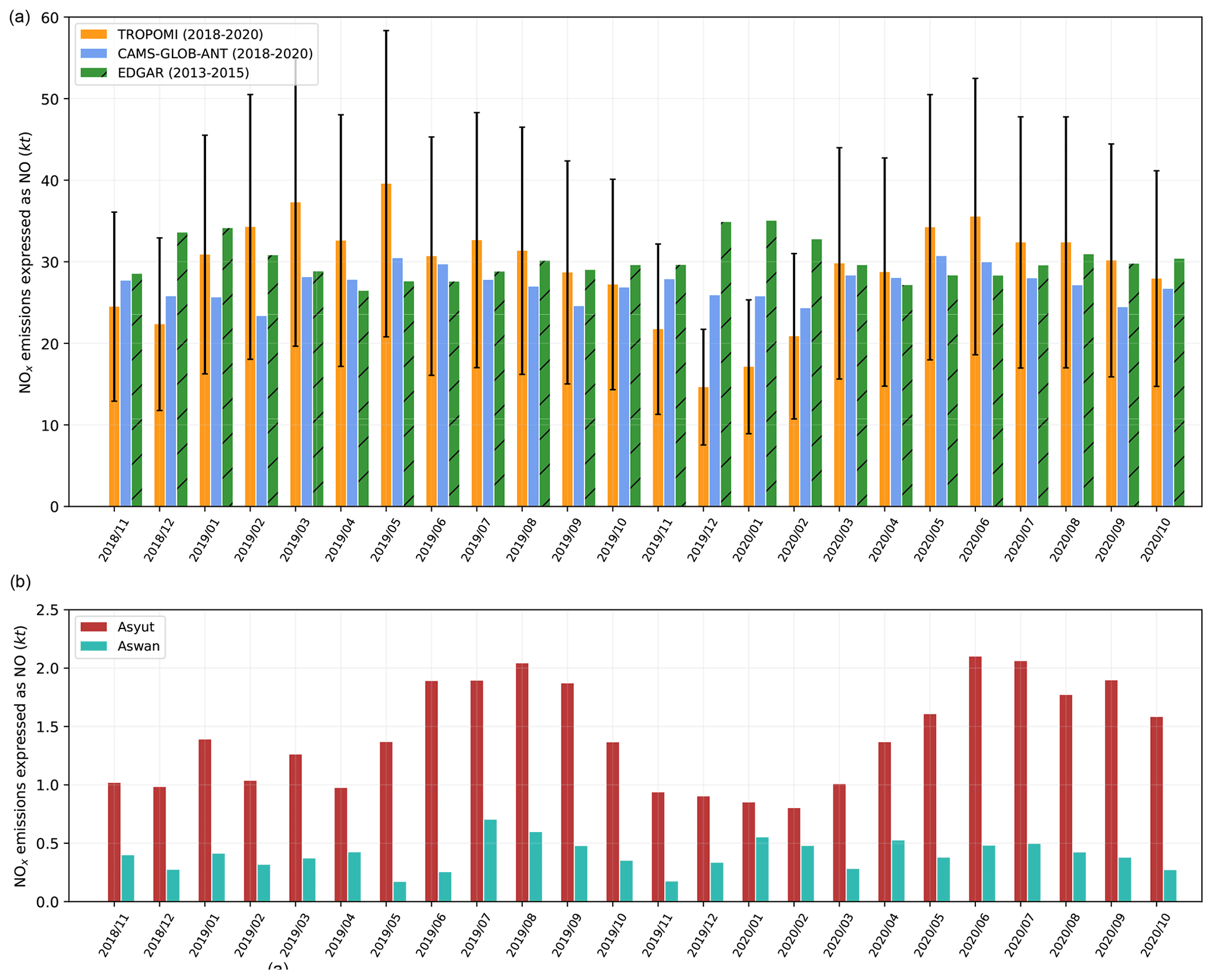
Figure 9(a) Comparison of TROPOMI-derived anthropogenic NOx emissions in Egypt (light blue), with the corresponding emissions from EDGAR (green with stripes) and CAMS (yellow) inventories. EDGAR data are shown for comparison purposes and cover the years 2013–2015. (b) TROPOMI-derived anthropogenic NOx emissions for the cities of Asyut (dark red) and Aswan (light blue). The corresponding domains are displayed in Fig. 1.
TROPOMI-derived emissions are higher than the CAMS inventory estimates. The top-down model estimates total NOx emissions of 697.6 kt over the 24 months, which is 45.9 kt higher than CAMS for the same period (651.6 kt). This difference is primarily localised in the first 12 months, for which TROPOMI-inferred emissions are always higher than the inventories and show higher values in summer than during the rest of the year. The next 12 months show similar emissions in summer but much lower values in winter. In particular, the difference is significant in December 2019 and January 2020 (respectively 56.5 % and 66.5 % of CAMS levels). These emissions also contrast with other winter emissions, with a total of 31.7 kt for December 2019–January 2020 against 53.3 kt for December 2018–January 2019 and 57.7 kt for December 2020–January 2021. In the computations, this drop for winter 2019/20 is mainly due to a relatively low value of the OH concentration, which reaches 4.61×10⁶ molec. cm−3 on average for December 2019 and January 2020, with 4.29×10⁶ molec. cm−3 above mask cells and 4.69×10⁶ molec. cm−3 over background cells. They were respectively 5.29, 5.74 and 5.18×10⁶ molec. cm−3 for the previous year (December 2018–January 2019) and 5.11, 4.90 and 5.16×10⁶ molec. cm−3 for the subsequent year (December 2020–January 2021). A decrease in tropospheric columns (−18.5 % for mask cells and −7.6 % for background cells compared to winter 2018/19) also contributes to this drop. The accuracy of the inferred emissions for winter 2019/20 can therefore be questioned.
At first sight, the annual variability of TROPOMI-inferred emissions, which describes a 1-year cycle with higher emissions in summer, seems to be correlated with power emissions which dominate the use of fossil fuels in Egypt (Abdallah and El-Shennawy, 2020). These power emissions are due to the country's residential electricity consumption (Attia et al., 2012; Elharidi et al., 2013; Nassief, 2014). They also meet the needs of industry. Summer peaks in electricity consumption are mostly driven by temperature, as illustrated by the increasing sales of air conditioning and ventilation systems for several decades (Wahba et al., 2018). The use of air conditioning in cars, which requires an additional amount of fuel, could also contribute to the increase in NOx emissions in summer. To support this hypothesis, we use our model on two smaller domains centred around the two cities of Asyut and Aswan. The corresponding domains are displayed in Fig. 1. Both cities have similar demographic features, with populations of about 467 000 and 315 000 inhabitants in 2021 and human densities of about 3000 and 1600 inhabitants per square kilometre respectively. However, their industrial features largely differ. There is no large fossil-fuel-fired power plant in Aswan, where most of the electricity is produced by a hydroelectric dam, whereas Asyut counts three oil and gas power plants of various capacities (90, 650 and 1500 MW) in its urban area. Both cities have a cement plant, but the one in Asyut has a larger production capacity (5.7 Mt yr−1 in Asyut, 0.8 Mt yr−1 in Aswan). Our model is used following the same procedure as for the main domain. The background removal is done at the scale of the country. A seasonal cycle appears for Asyut, with a minimum for winter months and a maximum for summer months. This cycle seems slightly shifted from the one observed for the entire country, for which May emissions are as important as those of summer months. We also note that the decrease in emissions for winter 2019/20 is less marked than for the emissions of the whole country, and of a similar value to the previous winter. This suggests that national NOx emissions are indeed lower during winter, but that the values obtained for winter 2019/20 are particularly low. We also find that the seasonality of the emissions is more pronounced for the Asyut domain than for the country as a whole. The case of Aswan is different. Emissions within the corresponding domain are significantly lower than for Asyut. The signal-to-noise ratio being higher, it is difficult to characterise an annual cycle, but the results do not seem to indicate low emissions in winter and high emissions in summer. This identification of a seasonal cycle identical to that of the entire country for a city with several power plants, and the absence of such a cycle in a city without any, strengthens the hypothesis that the power sector plays a major role in Egyptian NOx emissions.
We note that some features of the industrial activities in the country might be counteracting this trend. For some sectors such as cement or steel, production is lower in summer, due to the physical wear experienced by workers due to heat, but also due to certain periods of leave. Given the importance of industrial activities in the production of NOx shown in Sect. 4.2, this aspect cannot be neglected. The transport sector could also counteract the observed trend: although the use of air conditioning in cars increases NOx emissions of the sector, the observed mean traffic in the country is higher between November and February and lower between June and August, especially in Cairo, which includes most of the population. In the absence of additional data, it therefore seems difficult to conclude on the amplitude of the seasonal cycle produced by our top-down model. This caution is all the more necessary as CAMS and EDGAR show seasonal cycles for NOx emissions, with different dynamics than those displayed by TROPOMI emissions: while the EDGAR inventory predicts a maximum of emissions in December or January and a minimum in April, the CAMS inventory shows two local maxima each year in May and November and two local minima in February and September. The amplitude of the corresponding cycles is much lower in those inventories, representing 14.2 % of the average value for emissions estimates for EDGAR and 12.4% for CAMS. Those values must be compared to the amplitude displayed by TROPOMI-inferred emissions, for which the maximum-to-minimum ratio is about 1.8 if winter 2019/20 is excluded and 2.7 if it is included.
4.7 Uncertainties and assessments of results
The estimation of NOx emissions is based on the use of several quantities with varying uncertainties. The error bars shown in Figs. 5 and 9 are thus calculated from uncertainty statistics whose references are presented in this section. Since these references do not specify the exact nature of these statistics, we assume they correspond to standard deviations. The uncertainty of tropospheric NO2 columns under polluted conditions is dominated by the sensitivity of satellite observations to lower tropospheric air masses, expressed by the tropospheric air-mass factor (AMF). The column relative uncertainty due to the AMF is of the order of 30 % (Boersma et al., 2004). S-5P validation activities indicate that TROPOMI tropospheric NO2 columns are systematically biased low by about 30 %–50 % over cities (Verhoelst et al., 2021), which is most likely related to the a priori profiles used within the operational retrieval that do not reflect the NO2 peak close to ground well. For the Middle East region, the impact of the a priori profile is less critical, as surface albedo is generally high and cloud fractions are generally low. Thus, we expect no such bias and consider a relative uncertainty of 30 % for the tropospheric column. Other uncertainties must be taken into account: the transition from NO2 TROPOMI columns to NOx emissions requires parameters which appear in Eqs. (2) and (3). For the wind module, uncertainties are generally of about 1 m s−1 for components taken at precise altitudes (Coburn, 2019; Beirle et al., 2019). Here, we assume an uncertainty of 3 m s−1 for both zonal and meridional wind components. For [OH], the analysis of different methods conducted by Huijnen et al. (2019) showed smaller differences for low latitudes than for extratropics, but still significant. We thus take a relative uncertainty of 30 % for OH concentration. For the reaction rate kmean, the value of the corresponding relative uncertainty has been estimated by Burkholder et al. (2020). Finally, we use the sensitivity tests performed in Sect. 4.3 to assess the uncertainty associated with the choice of the vertical level. The cumulative effects on the final emissions of the three parameters studied, in particular the OH concentration, lead to a relative uncertainty that varies from month to month between 7 % and 18 %. The propagation of these different uncertainties on the monthly estimates of NOx emissions in Egypt leads to an expanded uncertainty between 47 % and 51 %. For lifetimes calculated with the EMG function fitting, the corresponding expanded uncertainty ranges between 18 % and 79 %.
We acknowledge the fact that our treatment of NOx is simplified. Many minor sinks highlighted in Sect. 3.1 are not taken into account. In particular, anthropogenic VOC emissions, which remove NOx from the atmosphere, compete with the oxidation by OH for the representation of NOx loss. These emissions are difficult to estimate, and the corresponding sink is complex to model. Taking this reaction into account would a priori lead to a strengthening of the sink term and thus to an increase in the NOx emissions estimates. Moreover, due to the coarse resolution of CAMS data, OH gradients might also be underestimated, especially in the southern part of the domain, leading to a local under-estimation of the sink term and the corresponding emissions. Other assumptions in the model are also simplifications. For instance, obtaining anthropogenic emissions by subtracting the average emissions over background cells assumes that the non-anthropogenic sources of NO2 are similar inside and outside the mask, which is not true, since a large part of the mask cells correspond to croplands. For these cells, soil emissions may play a non-negligible role in the natural NO2 budget. As a consequence, mean background emissions that are removed from NOx emissions estimates above mask cells might be under-estimated. Finally, the reliability of the data used can be questioned. The representation of the wind is crucial to avoid creating artificial patterns in the transport term. The OH concentration, which is proportional to the intensity of the sink term, is also important. We have shown that OH concentrations are partially responsible for an important drop in NOx emissions in the winter of 2019/20 that may be unrealistic. Because this decrease is largely due to variations in OH concentrations provided by CAMS, whose reliability has been evaluated for Riyadh, the transposability hypothesis between Riyadh and Egypt may be subject to further discussion.
In this study, we investigated the potential of a top-down model of NOx emissions based on TROPOMI retrievals at high resolution over Egypt. The model is based on the study of a transport term and a sink term that require different parameters to be calculated. Among those parameters, the concentration of OH, involved in the calculation of the NO2 mixed lifetime, is of fundamental importance. The comparison between NO2 lifetimes derived from OH concentrations and NO2 lifetimes derived from EMG function fittings of line density profiles shows that the OH concentration provided by CAMS is reasonably reliable for the country. Parameters are taken in the first 200 m of the planetary boundary layer, because it is where OH shows the best consistency. However, the vertical sensitivity linked to this parameter remains high. Results illustrate the importance of the transport term at a local scale, which is of the same order of magnitude as the sink term above large cities and industrial facilities; it ceases to be relevant only at the scale of the whole country. The top-down model is able to characterise declines in human activities due to restrictions during the COVID-19 pandemic or to Friday rest. It also estimates higher emissions during summer. These high emissions may be interpreted by a higher consumption of electricity driven by air-conditioning during hot days, but it remains unclear whether this pattern clearly reproduces changes in human activity, in particular because the emission inventories show different seasonalities. These inventories also differ in the amount of total emissions: the average value for TROPOMI-derived NOx emissions is 7.0 % higher than CAMS-GLOB-ANT_v4.2 estimates. This discrepancy could be resolved by comparing the results of the model and inventory estimates to industrial production or electricity consumption data at the scale of countries or regions.
Here, our estimation of NOx emissions benefited from favourable conditions. Egypt has a desertic climate, allowing us to neglect many NOx loss mechanisms for the sink term calculation, a flat terrain in most of its territory, limiting wind field errors for the transport term calculation and a large population concentrated in a small number of cities, providing NO2 maps with large signal-to-noise ratios above urban and industrial areas. For other regions of the world that do not have such features, the method presented here must be modified accordingly. However, we expect this method to be applicable to most countries similar to Egypt without substantial changes. For Middle East countries, this study thus demonstrates the potential of TROPOMI data for evaluating NOx emissions. More generally, it demonstrates the importance of the contribution of independent observation systems to overcome the weaknesses of emission inventories, provided that the local chemistry is well understood and modelled. The development of similar applications for different species is likely to allow a better monitoring of global anthropogenic emissions, therefore helping companies and countries to report their emissions of air pollutants and greenhouse gases as part of their strategies and obligations to tackle air pollution issues and climate change.
The software code for this research is not in a stand-alone user-friendly form but can be shared on request to the authors.
The TROPOMI NO2 product is publicly available on the TROPOMI Open hub (http://www.tropomi.eu/data-products/data-access, TROPOMI Data Hub, 2022). The offline mode (OFFL) data of version 1.0.0 to version 1.1.0 were used. CAMS data can be downloaded from the Copernicus Climate Data Store (https://ads.atmosphere.copernicus.eu/cdsapp#!/dataset/cams-global-atmospheric-composition-forecasts, ECMWF, 2022a). The European Centre for Medium-Range Weather Forecasts (ECMWF) ERA5 reanalysis be downloaded from the Copernicus Climate Data Store (https://cds.climate.copernicus.eu/cdsapp#!/dataset/reanalysis-era5-pressure-levels-monthly-means, ECMWF, 2022b). The Global Rural-Urban Mapping Project (GRUMP) dataset is available from the NASA Socioeconomic Data and Applications Center at https://sedac.ciesin.columbia.edu/data/collection/grump-v1 (SEDAC, 2017). Ground data for Egypt can be taken from http://globalenergyobservatory.org/ (Global Energy Observatory, 2022) for oil and gas power plants and from https://eogdata.mines.edu/download_global_flare.html (Earth Observation Group, 2021) for flaring sites. CAMS-GLOB-ANT_v4.2 data are available at https://eccad3.sedoo.fr/#CAMS-GLOB-ANT (ECCAD-AERIS, 2022). EDGAR v5.0 Global Air Pollutant Emissions are provided by https://edgar.jrc.ec.europa.eu/overview.php?v=50_AP (European Commission, 2022).
AR analysed the data, prepared the main software code and wrote the paper. FC provided the TROPOMI NO2 data product and corresponding gridded maps. PC contributed to building the database of emitters for Egypt. DH contributed to the interpretation of the use of OH for NOx loss. GB, TC, JK and JS contributed to the improvement of the method and the interpretation of the results. All authors read and agreed on the published version of the paper.
The contact author has declared that none of the authors has any competing interests.
Publisher's note: Copernicus Publications remains neutral with regard to jurisdictional claims in published maps and institutional affiliations.
The authors would like to thank Steven J. Davis (University of California, Irvine) and Dan Tong (Tsinghua University) for their contribution to the construction of our emitter database.
This research has been supported by the Horizon 2020 (EMME-CARE (grant no. 856612)).
This paper was edited by Bryan N. Duncan and reviewed by two anonymous referees.
Abdallah, L. and El-Shennawy, T.: Evaluation of CO2 emission from Egypt's future power plants, Euro-Mediterran. J. Environm. Integrat., 5, 1–8, 2020. a
Abou El-Magd, I. and Zanaty, N.: Impacts of short-term lockdown during COVID-19 on air quality in Egypt, Egypt. J. Remote Sens. Space Sci., 24, 493–500, 2020. a
Attia, S., Evrard, A., and Gratia, E.: Development of benchmark models for the Egyptian residential buildings sector, Appl. Energy, 94, 270–284, 2012. a, b
Baklanov, A., Molina, L. T., and Gauss, M.: Megacities, air quality and climate, Atmos. Environ., 126, 235–249, 2016. a
Bauwens, M., Compernolle, S., Stavrakou, T., Müller, J. F., Gent, J., Eskes, H., Levelt, P. F., A, R., Veefkind, J. P., Vlietinck, J., Yu, H., and Zehner, C.: Impact of coronavirus outbreak on NO2 pollution assessed using TROPOMI and OMI observations, Geophys. Res. Lett., 47, e2020GL087978, https://doi.org/10.1029/2020gl087978, 2020. a
Beirle, S., Boersma, K. F., Platt, U., Lawrence, M. G., and Wagner, T.: Megacity emissions and lifetimes of nitrogen oxides probed from space, Science, 333,1737–1739, 2011. a
Beirle, S., Borger, C., Dörner, S., Li, A., Hu, Z., Liu, F., Wang, Y., and Wagner, T.: Pinpointing nitrogen oxide emissions from space, Sci. Adv., 5, eaax9800, https://doi.org/10.1126/sciadv.aax9800, 2019. a, b, c, d, e, f, g
Beirle, S., Borger, C., Dörner, S., Eskes, H., Kumar, V., de Laat, A., and Wagner, T.: Catalog of NOx emissions from point sources as derived from the divergence of the NO2 flux for TROPOMI, Earth Syst. Sci. Data, 13, 2995–3012, https://doi.org/10.5194/essd-13-2995-2021, 2021. a
Boersma, K., Eskes, H., and Brinksma, E.: Error analysis for tropospheric NO2 retrieval from space, J. Geophys. Res.-Atmos., 109, D04311, https://doi.org/10.1029/2003JD003962, 2004. a, b
Burkholder, J., Sander, S., Abbatt, J., Barker, J., Cappa, C., Crounse, J., Dibble, T., Huie, R., Kolb, C., Kurylo, M., Orkin, V. L., Percival, C. J., Wilmouth, D. M., and Wine, P. H.: : Chemical kinetics and photochemical data for use in atmospheric studies; evaluation number 19. Technical report, Jet Propulsion Laboratory, National Aeronautics and Space, Pasadena, CA, http://jpldataeval.jpl.nasa.gov (last access: 23 August 2022), 2020. a, b, c, d, e
Butkovskaya, N., Kukui, A., Pouvesle, N., and Le Bras, G.: Formation of nitric acid in the gas-phase HO2 + NO reaction: Effects of temperature and water vapor, J. Phys. Chem. A, 109, 6509–6520, 2005. a, b
Butkovskaya, N., Rayez, M.-T., Rayez, J.-C., Kukui, A., and Le Bras, G.: Water vapor effect on the HNO3 yield in the HO2 + NO reaction: experimental and theoretical evidence, J. Phys. Chem. A, 113, 11327–11342, 2009. a
CIESIN: CIESIN. Global Rural-Urban Mapping Project, Version 1 (GRUMPv1), CIESIN – Center for International Earth Science Information Network, Columbia University, IFPRI – International Food Policy Research Institute, , The World Bank, and CIAT – Centro Internacional de Agricultura Tropical – SEDAC – Socioeconomic Data and Applications Center, NASA, Palisades, NY, https://doi.org/10.7927/H4R20Z93 (last access: 2 May 2022), 2019. a
Coburn, J. J.: Assessing wind data from reanalyses for the upper midwest, J. Appl. Meteorol. Clim., 58, 429–446, 2019. a
Crippa, M., Janssens-Maenhout, G., Dentener, F., Guizzardi, D., Sindelarova, K., Muntean, M., Van Dingenen, R., and Granier, C.: Forty years of improvements in European air quality: regional policy-industry interactions with global impacts, Atmos. Chem. Phys., 16, 3825–3841, https://doi.org/10.5194/acp-16-3825-2016, 2016. a
Crippa, M., Guizzardi, D., Muntean, M., Schaaf, E., Solazzo, E., Monforti-Ferrario, F., Olivier, J., and Vignati, E.: Fossil CO2 emissions of all world countries, European Commission, Luxembourg, 1–244, https://doi.org/10.2760/143674, 2020. a
de Foy, B., Lu, Z., Streets, D. G., Lamsal, L. N., and Duncan, B. N.: Estimates of power plant NOx emissions and lifetimes from OMI NO2 satellite retrievals, Atmos. Environ., 116, 1–11, 2015. a
Delaria, E. R., Place, B. K., Liu, A. X., and Cohen, R. C.: Laboratory measurements of stomatal NO2 deposition to native California trees and the role of forests in the NOx cycle, Atmos. Chem. Phys., 20, 14023–14041, https://doi.org/10.5194/acp-20-14023-2020, 2020. a
Earth Observation Group: flaring sites, https://eogdata.mines.edu/download_global_flare.html, last access: 16 July 2021. a
ECCAD-AERIS: CAMS-GLOB-ANT_v4.2 data [data set], https://eccad3.sedoo.fr/#CAMS-GLOB-ANT, last access: 6 July 2022. a
ECMWF: CAMS data, Copernicus Climate Data Store [data set], https://ads.atmosphere.copernicus.eu/cdsapp#!/dataset/cams-global-atmospheric-composition-forecasts, last access: 15 March 2022a. a
ECMWF: ERA5 reanalysis, Copernicus Climate Data Store [data set], https://cds.climate.copernicus.eu/cdsapp#!/dataset/reanalysis-era5-pressure-levels-monthly-means, last access: 15 March 2022b. a
EEHC: Egyptian Electricity Holding Company annual report 2019/2020, http://www.moee.gov.eg/english_new/report.aspx (last access: 23 August 2022), 2021. a
Ehhalt, D. H., Rohrer, F., and Wahner, A.: Sources and distribution of NOx in the upper troposphere at northern mid-latitudes, J. Geophys. Res.-Atmos., 97, 3725–3738, 1992. a
Elharidi, A. M. A. H., Tuohy, P. G., and Teamah, M.: Facing the growing problem of the electric power consumption in Egyptian residential building using building performance simulation program, in: Building simulation Cairo 2013 Conference – Towards Sustainable & Green Built Environment, Cairo, 23–24 June 2013, ID code: 46716, https://strathprints.strath.ac.uk/id/eprint/46716 (last access: 31 August 2022), 2013. a
El-Magd, I. A., Zanaty, N., Ali, E. M., Irie, H., and Abdelkader, A. I.: Investigation of aerosol climatology, optical characteristics and variability over Egypt based on satellite observations and in-situ measurements, Atmosphere, 11, 714, https://doi.org/10.3390/atmos11070714, 2020. a
El-Sheekh, M. M. and Hassan, I. A.: Lockdowns and reduction of economic activities during the COVID-19 pandemic improved air quality in Alexandria, Egypt, Environ. Monit. Assess., 193, 1–7, 2021. a
Elvidge, C. D., Zhizhin, M., Baugh, K., Hsu, F. C., and Ghosh, T.: Methods for global survey of natural gas flaring from visible infrared imaging radiometer suite data, Energies, 9, 14, https://doi.org/10.3390/en9010014, 2016. a
EPA: Integrated science assessment for oxides of nitrogen–health criteria, US Environmental Protection Agency, Washington, DC, https://cfpub.epa.gov/ncea/isa/recordisplay.cfm?deid=310879 (last access: 23 August 2022), 2016. a
European Commission: EDGAR v5.0 Global Air Pollutant Emissions [data set], https://edgar.jrc.ec.europa.eu/dataset_ap50, last access: 12 January 2022. a
Eskes, H., Eichmann, K., Lambert, J., Loyola, D., Veefkind, J., Dehn, A., and Zehner, C.: S5P Mission Performance Centre Nitrogen Dioxide [L2_NO2] readme, version 1, Royal Netherlands Meteorological Institute (KNMI), De Bilt, the Netherlands, http://www.tropomi.eu/sites/default/files/files/publicSentinel-5P-Nitrogen-Dioxide-Level-2-Product-Readme-File_20191105.pdf (last access: 23 August 2022), 2019. a
Fang, H., Baret, F., Plummer, S., and Schaepman-Strub, G.: An overview of global leaf area index (LAI): Methods, products, validation, and applications, Rev. Geophys., 57, 739–799, 2019. a
Filioglou, M., Giannakaki, E., Backman, J., Kesti, J., Hirsikko, A., Engelmann, R., O'Connor, E., Leskinen, J. T. T., Shang, X., Korhonen, H., Lihavainen, H., Romakkaniemi, S., and Komppula, M.: Optical and geometrical aerosol particle properties over the United Arab Emirates, Atmos. Chem. Phys., 20, 8909–8922, https://doi.org/10.5194/acp-20-8909-2020, 2020. a
Fischer, E. V., Jacob, D. J., Yantosca, R. M., Sulprizio, M. P., Millet, D. B., Mao, J., Paulot, F., Singh, H. B., Roiger, A., Ries, L., Talbot, R. W., Dzepina, K., and Pandey Deolal, S.: Atmospheric peroxyacetyl nitrate (PAN): a global budget and source attribution, Atmos. Chem. Phys., 14, 2679–2698, https://doi.org/10.5194/acp-14-2679-2014, 2014. a
Friedrich, N., Eger, P., Shenolikar, J., Sobanski, N., Schuladen, J., Dienhart, D., Hottmann, B., Tadic, I., Fischer, H., Martinez, M., Rohloff, R., Tauer, S., Harder, H., Pfannerstill, E. Y., Wang, N., Williams, J., Brooks, J., Drewnick, F., Su, H., Li, G., Cheng, Y., Lelieveld, J., and Crowley, J. N.: Reactive nitrogen around the Arabian Peninsula and in the Mediterranean Sea during the 2017 AQABA ship campaign, Atmos. Chem. Phys., 21, 7473–7498, https://doi.org/10.5194/acp-21-7473-2021, 2021. a, b
Gkatzelis, G. I., Gilman, J. B., Brown, S. S., Eskes, H., Gomes, A. R., Lange, A. C., McDonald, B. C., Peischl, J., Petzold, A., Thompson, C. R., and Kiendler-Scharr, A.: The global impacts of COVID-19 lockdowns on urban air pollution: A critical review and recommendations, Elem. Sci. Anth., 9, 00176, https://doi.org/10.1525/elementa.2021.00176, 2021. a
Global Energy Observatory: Ground data for Egypt [data set], http://globalenergyobservatory.org/, last access: 31 May 2022. a
Goldberg, D. L., Lu, Z., Streets, D. G., de Foy, B., Griffin, D., McLinden, C. A., Lamsal, L. N., Krotkov, N. A., and Eskes, H.: Enhanced Capabilities of TROPOMI NO2: Estimating NOx from North American Cities and Power Plants, Environ. Sci. Technol., 53, 12594–12601, 2019. a
Graedel, T., Farrow, L., and Weber, T.: Kinetic studies of the photochemistry of the urban troposphere, Atmos. Environ., 10, 1095–1116, 1976. a
Granier, C., Darras, S., Denier van der Gon, H. A. C., Doubalova, J., Elguindi, N., Galle, B., Gauss, M., Guevara, M., Jalkanen, J.-P., Kuenen, J., Liousse, C., Quack, B., Simpson, D., and Sindelarova, K.: The Copernicus atmosphere monitoring service global and regional emissions (April 2019 version), PhD thesis, Copernicus Atmosphere Monitoring Service, https://doi.org/10.24380/d0bn-kx16, 2019. a
Guenther, A., Karl, T., Harley, P., Wiedinmyer, C., Palmer, P. I., and Geron, C.: Estimates of global terrestrial isoprene emissions using MEGAN (Model of Emissions of Gases and Aerosols from Nature), Atmos. Chem. Phys., 6, 3181–3210, https://doi.org/10.5194/acp-6-3181-2006, 2006. a
Hale, T., Angrist, N., Goldszmidt, R., Kira, B., Petherick, A., Phillips, T., Webster, S., Cameron-Blake, E., Hallas, L., Majumdar, S., and Tatlow, H.: A global panel database of pandemic policies (oxford covid-19 government response tracker), Nat. Human Behav., 5, 529–538, 2021. a
Hersbach, H., Bell, B., Berrisford, P., Hirahara, S., Horányi, A., Muñoz-Sabater, J., Nicolas, J., Peubey, C., Radu, R., Schepers, D., Simmons, A., Soci, C., Abdalla, S., Abellan, X., Balsamo, G., Bechtold, P., Biavati, G., Bidlot, J., Bonavita, M., De Chiara, G., Dahlgren, P., Dee, D., Diamantakis, M., Dragani, R., Flemming, J., Forbes, R., Fuentes, M., Geer, A., Haimberger, L., Healy, S., Hogan, R. J., Hólm, E., Janisková, M., Keeley, S., Laloyaux, P., Lopez, P., Lupu, C., Radnoti, G., de Rosnay, P., Rozum, I., Vamborg, F., Villaume, S., and Thépaut, J.-N.: The ERA5 global reanalysis, Q. J. Roy. Meteorol. Soc., 146, 1999–2049, 2020. a
Hoelzemann, J. J., Schultz, M. G., Brasseur, G. P., Granier, C., and Simon, M.: Global wildland fire emission model (GWEM): Evaluating the use of global area burnt satellite data, J. Geophys. Res.-Atmos., 109, https://doi.org/10.1029/2003JD003666, 2004. a
Hoesly, R. M., Smith, S. J., Feng, L., Klimont, Z., Janssens-Maenhout, G., Pitkanen, T., Seibert, J. J., Vu, L., Andres, R. J., Bolt, R. M., Bond, T. C., Dawidowski, L., Kholod, N., Kurokawa, J.-I., Li, M., Liu, L., Lu, Z., Moura, M. C. P., O'Rourke, P. R., and Zhang, Q.: Historical (1750–2014) anthropogenic emissions of reactive gases and aerosols from the Community Emissions Data System (CEDS), Geosci. Model Dev., 11, 369–408, https://doi.org/10.5194/gmd-11-369-2018, 2018. a
Huijnen, V., Eskes, H., Wagner, A., Schulz, M., Christophe, Y., Ramonet, M., Basart, S., Benedictow, A., Blechschmidt, A.-M., Chabrillat, S., Clark, H., Cuevas, E., Flentje, H., Hansen, K. M., Im, U., Kapsomenakis, J., Langerock, B., Richter, A., Sudarchikova, N., Thouret, V., Warneke, T., and Zerefos, C.: Validation report of the CAMS near-real-time global atmospheric composition service: System evolution and performance statistics, Status up to 1 June 2016, https://pure.mpg.de/rest/items/item_2441827/component/file_2441834/content (last access: 23 August 2022), 2016. a
Huijnen, V., Pozzer, A., Arteta, J., Brasseur, G., Bouarar, I., Chabrillat, S., Christophe, Y., Doumbia, T., Flemming, J., Guth, J., Josse, B., Karydis, V. A., Marécal, V., and Pelletier, S.: Quantifying uncertainties due to chemistry modelling – evaluation of tropospheric composition simulations in the CAMS model (cycle 43R1), Geosci. Model Dev., 12, 1725–1752, https://doi.org/10.5194/gmd-12-1725-2019, 2019. a
IEA: Global energy review 2020, https://www.iea.org/, last access: 10 September 2020. a
Jaeglé, L., Steinberger, L., Martin, R. V., and Chance, K.: Global partitioning of NOx sources using satellite observations: Relative roles of fossil fuel combustion, biomass burning and soil emissions, Faraday Discuss., 130, 407–423, 2005. a
Janssens-Maenhout, G., Crippa, M., Guizzardi, D., Muntean, M., Schaaf, E., Dentener, F., Bergamaschi, P., Pagliari, V., Olivier, J. G. J., Peters, J. A. H. W., van Aardenne, J. A., Monni, S., Doering, U., Petrescu, A. M. R., Solazzo, E., and Oreggioni, G. D.: EDGAR v4.3.2 Global Atlas of the three major greenhouse gas emissions for the period 1970–2012, Earth Syst. Sci. Data, 11, 959–1002, https://doi.org/10.5194/essd-11-959-2019, 2019. a
Khoder, M.: Diurnal, seasonal and weekdays–weekends variations of ground level ozone concentrations in an urban area in greater cairo, Environ. Monit. Assess., 149, 349–362, 2009. a
Kim, H. C., Bae, C., Bae, M., Kim, O., Kim, B.-U., Yoo, C., Park, J., Choi, J., Lee, J.-b., Lefer, B., Stein, and A., Kim, S.: Space-Borne monitoring of NOx emissions from cement kilns in South Korea, Atmosphere, 11, 881, https://doi.org/10.3390/atmos11080881, 2020. a
Lama, S., Houweling, S., Boersma, K. F., Eskes, H., Aben, I., Denier van der Gon, H. A. C., Krol, M. C., Dolman, H., Borsdorff, T., and Lorente, A.: Quantifying burning efficiency in megacities using the ratio from the Tropospheric Monitoring Instrument (TROPOMI), Atmos. Chem. Phys., 20, 10295–10310, https://doi.org/10.5194/acp-20-10295-2020, 2020. a, b
Lange, K., Richter, A., and Burrows, J. P.: Variability of nitrogen oxide emission fluxes and lifetimes estimated from Sentinel-5P TROPOMI observations, Atmos. Chem. Phys., 22, 2745–2767, https://doi.org/10.5194/acp-22-2745-2022, 2022. a, b
Lelieveld, J., Gromov, S., Pozzer, A., and Taraborrelli, D.: Global tropospheric hydroxyl distribution, budget and reactivity, Atmos. Chem. Phys., 16, 12477–12493, https://doi.org/10.5194/acp-16-12477-2016, 2016. a
Leue, C., Wenig, M., Wagner, T., Klimm, O., Platt, U., and Jähne, B.: Quantitative analysis of NOx emissions from global ozone Monitoring Experiment satellite image sequences, J. Geophys. Res.-Atmos., 106, 5493–5505, 2001. a
Levy, H.: Normal atmosphere: Large radical and formaldehyde concentrations predicted, Science, 173, 141–143, 1971. a
Li, M., Karu, E., Brenninkmeijer, C., Fischer, H., Lelieveld, J., and Williams, J.: Tropospheric OH and stratospheric OH and Cl concentrations determined from CH4, CH3Cl, and SF6 measurements, NPJ Clim. Atmos. Sci., 1, 1–7, 2018. a
Lin, J.-T.: Satellite constraint for emissions of nitrogen oxides from anthropogenic, lightning and soil sources over East China on a high-resolution grid, Atmos. Chem. Phys., 12, 2881–2898, https://doi.org/10.5194/acp-12-2881-2012, 2012. a
Logan, J. A., Prather, M. J., Wofsy, S. C., and McElroy, M. B.: Tropospheric chemistry: a global perspective, J. Geophys. Res.-Oceans, 86, 7210–7254, 1981. a
Longfellow, C. A., Ravishankara, A., and Hanson, D. R.: Reactive uptake on hydrocarbon soot: Focus on NO2, J. Geophys. Res.-Atmos., 104, 13833–13840, 1999. a
Lorente, A., Folkert Boersma, K., Yu, H., Dörner, S., Hilboll, A., Richter, A., Liu, M., Lamsal, L. N., Barkley, M., De Smedt, I., Van Roozendael, M., Wang, Y., Wagner, T., Beirle, S., Lin, J.-T., Krotkov, N., Stammes, P., Wang, P., Eskes, H. J., and Krol, M.: Structural uncertainty in air mass factor calculation for NO2 and HCHO satellite retrievals, Atmos. Meas. Tech., 10, 759–782, https://doi.org/10.5194/amt-10-759-2017, 2017. a
Lorente, A., Boersma, K., Eskes, H., Veefkind, J., Van Geffen, J., De Zeeuw, M., van der Gon, H. D., Beirle, S., and Krol, M.: Quantification of nitrogen oxides emissions from build-up of pollution over Paris with TROPOMI, Scient. Rep., 9, 1–10, 2019. a, b
Martin, R. V., Jacob, D. J., Chance, K., Kurosu, T. P., Palmer, P. I., and Evans, M. J.: Global inventory of nitrogen oxide emissions constrained by space-based observations of NO2 columns, J. Geophys. Res.-Atmos., 108, D17, https://doi.org/10.1029/2003JD003453, 2003. a
Mijling, B. and Van Der A, R.: Using daily satellite observations to estimate emissions of short-lived air pollutants on a mesoscopic scale, J. Geophys. Res.-Atmos., 117, D17302, https://doi.org/10.1029/2012JD017817, 2012. a
Moxim, W., Levy, H., and Kasibhatla, P.: Simulated global tropospheric PAN: Its transport and impact on NOx, J. Geophys. Res.-Atmos., 101, 12621–12638, 1996. a
Müller, J.-F. and Stavrakou, T.: Inversion of CO and NOx emissions using the adjoint of the IMAGES model, Atmos. Chem. Phys., 5, 1157–1186, https://doi.org/10.5194/acp-5-1157-2005, 2005. a
Nassief, M. M.: Evaluation of electricity consumption of a residential flat in egypt, Am. J. Elect. Power Energ. Syst., 3, 7–44, 2014. a
Nault, B. A., Garland, C., Wooldridge, P. J., Brune, W. H., Campuzano-Jost, P., Crounse, J. D., Day, D. A., Dibb, J., Hall, S. R., Huey, L. G., Jimenez, J. L., Liu, X., Mao, J., Mikoviny, T., Peischl, J., Pollack, I. B., Ren, X., Ryerson, T. B., Scheuer, E., Ullmann, K., Wennberg, P. O., Wisthaler, A., Zhang, L., and Cohen, R. C.: Observational constraints on the oxidation of NOx in the upper troposphere, J. Phys. Chem. A, 120, 1468–1478, 2016. a
Rohrer, F. and Berresheim, H.: Strong correlation between levels of tropospheric hydroxyl radicals and solar ultraviolet radiation, Nature, 442, 184–187, 2006. a
Romer Present, P. S., Zare, A., and Cohen, R. C.: The changing role of organic nitrates in the removal and transport of NOx, Atmos. Chem. Phys., 20, 267–279, https://doi.org/10.5194/acp-20-267-2020, 2020. a, b
Sander, S. P., Abbatt, J., Barker, J. R., Burkholder, J. B., Friedl, R. R., Golden, D. M., Huie, R. E., Kolb, C. E., Kurylo, M. J., Moortgat, G. K., Orkin, V. L., and Wine, P. H.: Chemical Kinetics and Photochemical Data for Use in Atmospheric Studies, Evaluation No. 17, JPL Publication 10-6, Jet Propulsion Laboratory, Pasadena, 2011, http://jpldataeval.jpl.nasa.gov/pdf/JPL 10-6 Final 15June2011.pdf (last access: 28 August 2022), 2011. a
SEDAC: The Global Rural-Urban Mapping Project (GRUMP), NASA Socioeconomic Data and Applications Center [data set], https://sedac.ciesin.columbia.edu/data/collection/grump-v1 (last access: 2 May 2022), 2017. a
Seinfeld, J. H.: Urban air pollution: state of the science, Science, 243, 745–752, 1989. a, b, c
Seinfeld, J. H. and Pandis, S. N.: Atmospheric Chemistry and Physics: From Air Pollution to Climate Change, 2nd Edition, John Wiley & Sons, New York, ISBN-13: 978-0-471-72017-1, 2006. a
Singh, A. and Agrawal, M.: Acid rain and its ecological consequences, J. Environ. Biol., 29, 15–24, 2008. a
Sobanski, N., Thieser, J., Schuladen, J., Sauvage, C., Song, W., Williams, J., Lelieveld, J., and Crowley, J. N.: Day and night-time formation of organic nitrates at a forested mountain site in south-west Germany, Atmos. Chem. Phys., 17, 4115–4130, https://doi.org/10.5194/acp-17-4115-2017, 2017. a
Stavrakou, T., Müller, J.-F., Boersma, K. F., van der A, R. J., Kurokawa, J., Ohara, T., and Zhang, Q.: Key chemical NOx sink uncertainties and how they influence top-down emissions of nitrogen oxides, Atmos. Chem. Phys., 13, 9057–9082, https://doi.org/10.5194/acp-13-9057-2013, 2013. a
Stavrakou, T., Müller, J.-F., Bauwens, M., Boersma, K., and van Geffen, J.: Satellite evidence for changes in the NO2 weekly cycle over large cities, Scient. Rep., 10, 1–9, 2020. a
Tang, L., Xue, X., Jia, M., Jing, H., Wang, T., Zhen, R., Huang, M., Tian, J., Guo, J., Li, L., Bo, X., and Wang, S.: Iron and steel industry emissions and contribution to the air quality in China, Atmos. Environ,, 237, 117668, https://doi.org/10.1016/j.atmosenv.2020.117668, 2020. a
TROPOMI Data Hub: TROPOMI NO2 product, TROPOMI Open hub [data set], http://www.tropomi.eu/data-products/data-access, last access: 22 July 2022. a
UNEP: Air quality policies in Egypt, https://www.unep.org/resources/policy-and-strategy/air-quality-policies-egypt (last access: 23 August 2022), 2015. a
Valin, L., Russell, A., and Cohen, R.: Variations of OH radical in an urban plume inferred from NO2 column measurements, Geophys. Res. Lett., 40, 1856–1860, 2013. a, b, c
Valin, L. C., Russell, A. R., Hudman, R. C., and Cohen, R. C.: Effects of model resolution on the interpretation of satellite NO2 observations, Atmos. Chem. Phys., 11, 11647–11655, https://doi.org/10.5194/acp-11-11647-2011, 2011. a, b
Veefkind, J., Aben, I., McMullan, K., Förster, H., De Vries, J., Otter, G., Claas, J., Eskes, H., De Haan, J., Kleipool, Q., van Weele, M., Hasekamp, O., Hoogeveen, R., Landgraf, J., Snel, R., Tol, P., Ingmann, P., Voors, R., Kruizinga, B., Vink, R., Visser, H., and Levelt, P. F.: TROPOMI on the ESA Sentinel-5 Precursor: A GMES mission for global observations of the atmospheric composition for climate, air quality and ozone layer applications, Remote Sens. Environ., 120, 70–83, 2012. a
Venter, Z. S., Aunan, K., Chowdhury, S., and Lelieveld, J.: COVID-19 lockdowns cause global air pollution declines, P. Natl. Acad. Sci. USA, 117, 18984–18990, 2020. a
Verhoelst, T., Compernolle, S., Pinardi, G., Lambert, J.-C., Eskes, H. J., Eichmann, K.-U., Fjæraa, A. M., Granville, J., Niemeijer, S., Cede, A., Tiefengraber, M., Hendrick, F., Pazmiño, A., Bais, A., Bazureau, A., Boersma, K. F., Bognar, K., Dehn, A., Donner, S., Elokhov, A., Gebetsberger, M., Goutail, F., Grutter de la Mora, M., Gruzdev, A., Gratsea, M., Hansen, G. H., Irie, H., Jepsen, N., Kanaya, Y., Karagkiozidis, D., Kivi, R., Kreher, K., Levelt, P. F., Liu, C., Müller, M., Navarro Comas, M., Piters, A. J. M., Pommereau, J.-P., Portafaix, T., Prados-Roman, C., Puentedura, O., Querel, R., Remmers, J., Richter, A., Rimmer, J., Rivera Cárdenas, C., Saavedra de Miguel, L., Sinyakov, V. P., Stremme, W., Strong, K., Van Roozendael, M., Veefkind, J. P., Wagner, T., Wittrock, F., Yela González, M., and Zehner, C.: Ground-based validation of the Copernicus Sentinel-5P TROPOMI NO2 measurements with the NDACC ZSL-DOAS, MAX-DOAS and Pandonia global networks, Atmos. Meas. Tech., 14, 481–510, https://doi.org/10.5194/amt-14-481-2021, 2021. a
Wahba, S. M., Kamel, B. A., Nassar, K. M., and Abdelsalam, A. S.: Effectiveness of green roofs and green walls on energy consumption and indoor comfort in arid climates, Civ. Eng. J., 4, 2284–2295, 2018. a
Wiedinmyer, C., Tie, X., Guenther, A., Neilson, R., and Granier, C.: Future changes in biogenic isoprene emissions: how might they affect regional and global atmospheric chemistry?, Earth Interact., 10, 1–19, 2006. a
Wolfe, G. M., Nicely, J. M., Clair, J. M. S., Hanisco, T. F., Liao, J., Oman, L. D., Brune, W. B., Miller, D., Thames, A., Abad, G. G., Ryerson, T. B., Thompson, C. R., Peischl, J., McKain, K., Sweeney, C., Wennberg, P. O., Kim, M., Crounse, J. D., Hall, S. R., Ullmann, K., Diskin, G., Bui, P., Chang, C., and Dean-Day, J.: Mapping hydroxyl variability throughout the global remote troposphere via synthesis of airborne and satellite formaldehyde observations, P. Natl. Acad. Sci. USA, 116, 11171–11180, 2019. a
Xue, B. and Ren, W.: China's uncertain CO2 emissions, Nat. Clim. Change, 2, 762–762, 2012. a
Yienger, J. and Levy, H.: Empirical model of global soil-biogenic NOx emissions, J. Geophys. Res.-Atmos., 100, 11447–11464, 1995. a