the Creative Commons Attribution 4.0 License.
the Creative Commons Attribution 4.0 License.
 | 06 Sep 2022
Toward targeted observations of the meteorological initial state for improving the PM2.5 forecast of a heavy haze event that occurred in the Beijing–Tianjin–Hebei region
Lichao Yang
Wansuo Duan
Zifa Wang
Wenyi Yang
An advanced approach of conditional non-linear optimal perturbation (CNOP) was adopted to identify the sensitive area for targeted observations of meteorological fields associated with PM2.5 concentration forecasts of a heavy haze event that occurred in the Beijing–Tianjin–Hebei (BTH) region, China, from 30 November to 4 December 2017. The results show that a few specific regions in the southern and northwestern directions close to the BTH region represent the sensitive areas. Numerically, when predetermined artificial observing arrays (i.e. possible “targeted observations”) in the sensitive areas were assimilated, the forecast errors of PM2.5 during the accumulation and dissipation processes were aggressively reduced; specifically, these assimilations, compared with those in other areas that have been thought of as being important for the PM2.5 forecasts in the BTH region in previous studies, exhibited a more obvious decrease in the forecast errors of PM2.5. Physically, the reason why these possible targeted observations can significantly improve the forecasting skill of PM2.5 was interpreted by comparing relevant meteorological fields before and after assimilation. Therefore, we conclude that preferentially deploying additional observations in the sensitive areas identified by the CNOP approach can greatly improve the forecasting skill of PM2.5, which provides, beyond all doubt, theoretical guidance for practical field observations of meteorological fields associated with PM2.5 forecasts.
- Article
(24054 KB) - Full-text XML
- BibTeX
- EndNote


Air pollution is one of the most severe environmental problems that China is facing. Among various air pollutants, fine particulate matter (PM2.5) has been considered as the most serious pollutant, frequently engulfing northern China, including the Beijing–Tianjin–Hebei (BTH) region. Exposure to heavy PM2.5 episodes not only increases the risks of various respiratory diseases but also induces the possibility of diabetes and other metabolic-dysfunction-related diseases (Guan et al., 2016; Lim and Thurston, 2019). Accurate PM2.5 concentration forecasts are essential since they can remind people to reduce exposure during haze days and can assist policy-makers in making effective emission reduction measure decisions. The atmospheric chemical transport model (CTM) is one of the most widely used and effective ways to forecast PM2.5 concentrations. However, relevant chemical and physical processes are complex, and associated parameterization schemes of turbulent processes and meteorological and emission conditions cannot describe the real world exactly, causing model forecasts to have great uncertainty, especially on heavy haze days (Hu et al., 2010; Kong et al., 2021).
The uncertainties of CTM output, as mentioned above, are primarily attributed to the uncertainties of meteorological and emission inputs, in addition to those occurring in the chemical model formulation (Romano et al., 2004; Gilliam et al., 2015). Meteorological conditions, including wind, temperature and relative humidity, which are crucial for the transformation, formation, diffusion and removal of pollutants in the atmosphere, have a great impact on PM2.5 forecasts of the BTH region in CTMs (Godowitch et al., 2011; Chen et al., 2020). Using an artificial neural network model combined with wavelet transformation, He et al. (2017) demonstrated that meteorological conditions explained more than 70 % of the variance in daily PM2.5 concentrations over the major cities in China. Therefore, regional PM2.5 concentrations rely on meteorological variations to a large extent. Thus, to improve the PM2.5 forecasting skill, it is necessary to understand the sensitivity of the CTM results to the inputted meteorological fields and to reduce meteorological uncertainty. It has been demonstrated that uncertainties in the meteorological initial field substantially influence pollution simulations, including their temporal variations and peak time concentrations (Zhang et al., 2007; Bei et al., 2017; Liu et al., 2018). Thus, increasing the accuracy of the meteorological initial conditions is an effective way to improve the PM2.5 forecasting skill.
Data assimilation is recognized as a useful technique for improving the accuracy of initial conditions. To obtain reliable initial meteorological conditions, sufficient and effective observations are essential. However, conventional observations, which are distributed at a low resolution in both oceans and islands, have a limitation in improving the accuracy of initial conditions (Li et al., 2015). Assimilating additional field observations has been proven to be an effective way to obtain a reliable initial field (Snyder, 1996; Mu et al., 2015). Since field observations are costly and never sufficiently dense, one can consider placing a preferentially limited number of observations in key areas to have the most positive impacts on improving forecast skill. This idea is just one of the new observational strategies of “target observation”, also called “adaptive observation”, which has been developed over the past 2 decades (Snyder, 1996; Palmer et al., 1998; Majumdar, 2016). The target observation mainly serves the demand of forecasts on observations. The idea is as follows. To better predict an event at a future time t2 (i.e. verification time) in a focused area (i.e. verification area), additional observations are deployed at a future time t1 (i.e. target time; t1<t2) in some key areas (i.e. sensitive areas) where additional observations are expected to have a large contribution in reducing the prediction errors in the verification area. These additional observations are assimilated by a data assimilation system to provide a more reliable initial state, which would be supplied to the model to obtain a more accurate prediction. Targeted observations have become a hot topic in atmospheric science due to their successful applications in improving the prediction skills of extreme weather events, such as typhoons (Wu et al., 2009; Mu et al., 2009) and winter storms (Kren et al., 2020) and high-impact climatic events, such as the El Niño–Southern Oscillation (ENSO; Kramer and Dijkstra, 2013; Duan et al., 2018) and Indian Ocean Dipole (IOD; Feng et al., 2017; Beal et al., 2020). As we stated above, the meteorological initial fields have great impacts on the PM2.5 forecasts of the BTH region (Bei et al., 2017; Liu et al., 2018); meanwhile, our results also showed that the PM2.5 forecasts are sensitive to the uncertainties of meteorological initial conditions (see Sect. 3.1). Based on these findings, we would propose the following question: can we apply the targeted observation strategy to improve the meteorological condition forecasts, which then further improve the PM2.5 forecasts of BTH region? It has also been argued that sufficient satellite observations can be used to yield the meteorological initial field by using a data assimilation approach. However, assimilating more observations may not lead to higher forecast benefits. Therefore, even if there are sufficient observations, one should also consider which areas of observations and how many observations should be preferentially assimilated to improve the PM2.5 forecast skill to a larger degree. When the observations in the area with high sensitivity are assimilated to the initial values of the forecast, the forecasting skills will be greatly increased; conversely, if the observations in the area where the forecast is not sensitive to the initial values are assimilated, the forecasting skills will be improved slightly or even become worse (Yu et al., 2012; Janjić et al., 2018; Zhang et al., 2018). Thus, the present study will explore the relevant sensitive area and examine the role of possible targeted observations on meteorological fields in improving the PM2.5 forecast skill during a heavy haze event that occurred from 30 November to 4 December 2017 in the BTH region, eventually suggesting the usefulness of implementing targeted observations on meteorological fields for improving air quality forecasts.
The key for the targeted observation is the determination of sensitive areas mentioned above and the design of the observation network. That is, when implementing the targeted observations, one should first make clear where to preferentially implement targeted observations and how to display these additional observations. To obtain the sensitive areas of meteorological fields for PM2.5 forecasting, an advanced optimization method, conditional non-linear optimal perturbation (CNOP), is used (Mu et al., 2003; Mu and Zhang, 2006), which overcomes the linear limitation of the traditional singular-vector approach (Lorenz, 1965). The CNOP represents the initial perturbation that causes the largest error growth at a given future time over the verification area. The CNOP is therefore the most sensitive initial perturbation; therefore, it would have potential for providing the sensitive area for targeting observations. In fact, the CNOP has been adopted to identify sensitive areas for targeting observations in both observations system simulation experiments (OSSEs) and/or practical observation tasks associated with typhoons, ENSO, Kuroshio and marine environments over the coast of China (Mu et al., 2015; Da et al., 2019) and has gained great success in improving the forecasting skills of the concerned high-impact weather or climatic events.
In the present study, we would consider the importance of the meteorological initial conditions on PM2.5 forecasting and apply the targeted observation strategy of meteorological fields with the CNOP approach to study the PM2.5 forecast of a heavy haze episode. As mentioned above, during the period from 30 November to 4 December 2017, a heavy air pollution event occurred in the BTH region, with hourly maximum PM2.5 concentrations greater than 250 µg m−3, exceeding the standard of severe pollution (Feng et al., 2016). However, the Beijing Municipal Ecological and Environmental Monitoring Center did not provide a warning of this event in time (see the link http://www.bjmemc.com.cn/, last access: 30 August 2022). We utilize this event as an example to explore the possible targeted observations of meteorological fields and to investigate whether they can help improve the PM2.5 forecasting skill. Specifically, the following questions are addressed.
- a.
Which area represents the sensitive area of initial meteorological fields for targeted observations associated with the PM2.5 forecast of the concerned event?
- b.
What is the optimal observation array for targeted observations in meteorological fields (in terms of locations and coverage density)?
- c.
Why can the targeted observations in the sensitive areas lead to a larger improvement in the PM2.5 forecasting skill of the event?
The paper is organized as follows. The model, methodology and data used in the study are introduced in the next section. Then, the CNOP-type errors of the meteorological field forecasting of the haze event are calculated in Sect. 3. In Sect. 4, the sensitive areas of the meteorological field for the PM2.5 forecasts are identified, and relevant OSSEs are designed to verify the validity of the targeted observation in improving the forecasting skill of PM2.5 in the haze event. In Sect. 5, the reasons why the targeted observations can result in a larger improvement in PM2.5 forecasts are interpreted. Finally, a summary and discussion are presented in Sect. 6.
In this study, we adopt a nested air quality prediction modelling system (NAQPMS) and a weather research and forecasting (WRF) model to explore the role of targeted observations on meteorological fields in improving the surface air concentrations of PM2.5 forecasts by building an optimization problem associated with the CNOP approach.
2.1 Models
The NAQPMS is a three-dimensional regional Eulerian chemical transport model developed by the Institute of Atmospheric Physics, Chinese Academy of Sciences (Wang et al., 1997, 2006). It includes modules that address horizontal and vertical advection and diffusion, dry–wet deposition, gaseous phases, aqueous phases, aerosols, and heterogeneous chemical reactions. The NAQPMS has been widely applied to forecast air pollutants and to study the source apportionment of pollutants (Yang et al., 2020). The anthropogenic emissions of PM2.5 and other pollutants are from Multi-resolution Emission Inventory for China in 2017 (MEIC 2017) (Li et al., 2014) (http://meicmodel.org/, last access: 30 August 2022). The model integration is conducted in a single model domain of 95 × 95 grids at a resolution of 30 km with 20 vertical levels. The components of PM2.5 simulation include black carbon (BC), organic carbon (OC), secondary inorganic aerosol (sulfate, nitrate, ammonium) and primary PM2.5 emitted directly from various sources. The mass of aerosol liquid water is not included in the simulated PM2.5 mass concentrations so that the PM2.5 simulations are dry mass concentrations.
The NAQPMS is driven by the meteorological field generated through WRFV3.6.1 (https://www2.mmm.ucar.edu/wrf/users/, last access: 30 August 2022). The WRF model used in the present study adopts the Lin microphysics scheme (Lin et al., 1983), the Rapid Radiative Transfer Model for General circulation (RRTMG) longwave radiation scheme (Iacono et al., 2008), the Dudhia shortwave radiation scheme (Dudhia, 1989) and the Yonsei University planetary boundary layer parameterization scheme (Hong et al., 2006). These parameterization schemes are also adopted in the adjoint model of the WRF, which is used to calculate the CNOP (see Sect. 2.2). To enhance the computing efficiency of the CNOP, a horizonal resolution of 30 km is used in the present study for an initial attempt. The model domain of the WRF and its adjoint model are the same as in the NAQPMS. The assimilation system we used is a 3-D variational data assimilation system of the WRF, which has been proven to be an efficient assimilation tool for PM2.5 simulations (Kumar et al., 2019; Zhang et al., 2021).
2.2 Conditional non-linear optimal perturbation (CNOP)
The CNOP represents the initial perturbation (or error) that can lead to the largest forecast error in the focused area (verification area) at verification time. Suppose a non-linear model is expressed as Eq. (1),
where x is the state vector with an initial value x0 and F is a non-linear partial differential operator. The solution of Eq. (1) can be described as x(t)=M(x0), in which M is the non-linear propagator. If x(t) is a reference state and an initial perturbation δx0 is added to its initial state x0, a forecast will be made with , where represents the evolution of the initial perturbation δx0. Thus, an initial perturbation is CNOP () if and only if
where is the constraint condition that the initial perturbation should satisfy and β is a positive value that is comparable to the initial analysis error variance of the considered variables. C1 and C2 are coefficient matrices, which define the amplitudes of initial perturbations δx0 and its evolution , with x consisting of zonal and meridional wind (U and V, respectively), temperature (T), water vapour mixing ratio (Q), and pressure (P) components in the present study, and they play their role by calculating the total perturbation energy from surface to top (i.e. 100 hPa), as in Eq. (3) (Ehrendorfer et al., 1999; Chen et al., 2020).
Here, Cp (=1005.7 J kg−1 K−1), Ra (=287.04 J kg−1 K−1), Tr (=270 K), L (=2.5105 ×10⁶ J kg−1), and Pr (=1000 hPa) are constant values and U′, V′ T′, Q′, and P′ denote the perturbations superimposed on meteorological fields of zonal and meridional wind, temperature, water vapour mixing ratio, and pressure, respectively. D denotes the verification area, which is the BTH region in this study and η signifies the vertical coordinate.
The optimization problem in Eq. (2) is solved by using the spectral projected gradient 2 (SPG2) method (Birgin et al., 2001) in the present study. A first guess is assigned to the initial perturbation δx0. The WRF model is integrated forward with the initial state x0+δx0 to obtain the forecast M(x0+δx0). The cost function J is calculated by using M(x0+δx0) and M(x0). The adjoint model of the WRF is integrated backward to calculate the gradient of the cost function with respect to the initial perturbation δx0. The gradient represents the fastest descending direction of the cost function J in Eq. (2). Based on the iteratively forward and backward integration governed by the SPG2 algorithm, the initial perturbation δx0 is optimized and updated until the convergence condition of the algorithm is satisfied. Here, the convergence condition is , where ε1 is an extremely small positive number, P(δx0) projects the δx0 outside the constraint to the boundary of the constraint condition and g(δx0) represents the gradient of the cost function J with respect to δx0. Thus, the resultant initial perturbation is the CNOP. The details for the SPG2 algorithm can be seen in Birgin et al. (2001).
2.3 Data
Surface PM2.5 observation datasets for verification are obtained from national environmental monitoring stations. There are 1287 national stations across China, 80 of which are located in the BTH region. The distribution of the 80 observation sites within the BTH region is shown in Fig. 1. We retrieved the hourly measurements of PM2.5 from 80 air quality monitoring stations from 30 November to 4 December 2017, where the PM2.5 observations are for dry mass concentrations and there are no missing values during the time period we considered.
The fifth-generation ECMWF reanalysis for the global climate and weather (ERA5) (https://www.ecmwf.int/en/forecasts/datasets/reanalysis-datasets/era5, last access: 30 August 2022) and National Centers for Environmental Prediction (NCEP) Global Forecasting System (GFS) historical archive forecast data (GFS, https://rda.ucar.edu/ datasets/ds084.1/, last access: 30 August 2022) are both used to produce the initial and boundary meteorological conditions for the WRF simulations. Both the ERA5 and GFS data have a 0.25∘ spatial resolution (approximately 25 km) and 6 h temporal resolution.
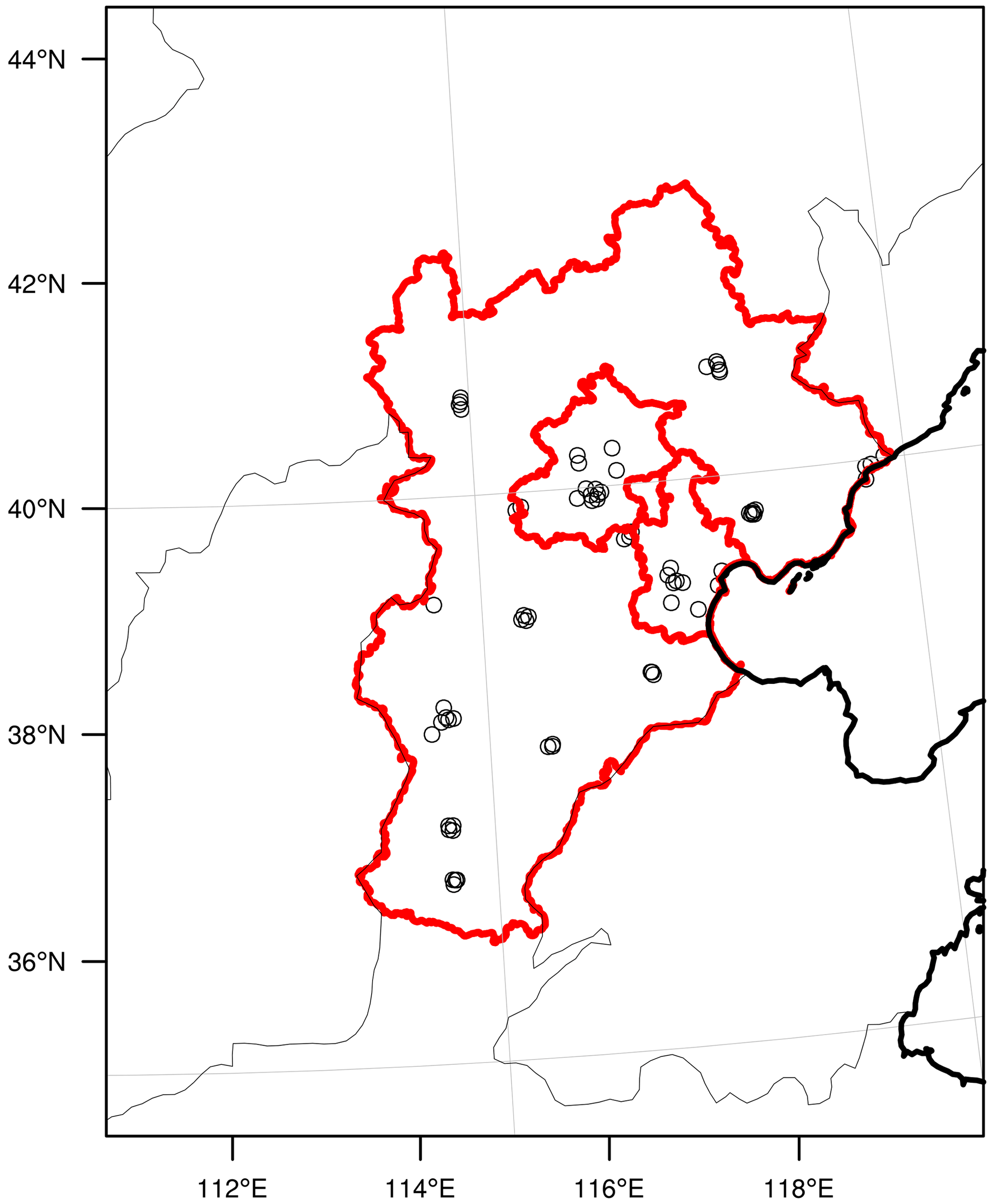
Figure 1Map of the current environmental monitoring stations (hollow circles) within the BTH domain. The thin black lines show the boundaries of the surrounding Chinese provinces, and the thick black lines show the coastline. The boundaries of Beijing, Tianjin and Hebei Province are marked in red.
In this section, we use the CNOP approach to identify the sensitive areas for targeted observations associated with the PM2.5 forecast in the heavy haze event in BTH that occurred from 30 November to 4 December 2017. Figure 2a and b plot the time series of the PM2.5 concentration observed at the Baoding (in Hebei) and Dongsi (in Beijing) environmental monitoring stations. The haze started to develop at approximately 02:00 BJT (Beijing time, UTC + 8 h) on 1 December and dispersed at 14:00 BJT on 3 December. Specifically, the PM2.5 concentrations of most cities in the BTH region exceeded 250 µg m−3 at 12:00 BJT on 2 December. Following this, starting from 01:00 BJT on 3 December, the PM2.5 dissipated rapidly within several hours. In Beijing, from 00:00 BJT on 1 December, it took almost 1 d to accumulate PM2.5 from 77 o 160 µg m−3 according to the Dongsi station. Finally, from 01:00 BJT on 3 December, the PM2.5 concentration decreased from 256 to 19 µg m−3 over 7 h.
3.1 Simulations of the PM2.5 variability in the heavy haze event
After a 10 d spin-up of the WRF-NAQPMS, the ERA5 and GFS meteorological data are separately adopted to initialize the WRF at 00:00 BJT on 30 November 2017, and the simulations of PM2.5 concentrations at the Baoding and Dongsi stations are plotted in Fig. 2. Since the two simulations are generated by the same model using the same emission inventory, the PM2.5 forecast uncertainties are only attributed to the uncertainties of meteorological initial fields. The simulation initialized by ERA5 can better reproduce the pollution event. During the period between 00:00 BJT on 30 November and 23:00 BJT on 1 December, the simulations initialized by ERA5 almost overlap with the observations. In the remaining time period, although the highest PM2.5 concentration simulated by ERA5 occurs approximately 12 h earlier and more than 50 µg m−3 lower than those in the observations, the simulation can represent the accumulation and dissipation processes of PM2.5 well.

Figure 2Time series of the dry PM2.5 concentrations at (a) Baoding station (Hebei Province) and (b) Dongsi station (Beijing) of observations and simulations initialized by ERA5 and GFS meteorological data during the period between 30 November and 4 December 2017. The accumulation time (AT) and dissipation time (DT) are marked by dashed lines.
The simulations initialized by the GFS do not perform well in representing the episode of PM2.5. They underestimate the PM2.5 concentrations during the accumulation process, and the simulated highest PM2.5 concentration (176 µg m−3) occurs at approximately 21:00 BJT on 3 December in Baoding, which is exactly in the dissipation process of the observed event. The simulation of Beijing PM2.5 also shows a large deviation from the observational PM2.5 concentration, especially during the dissipation process.
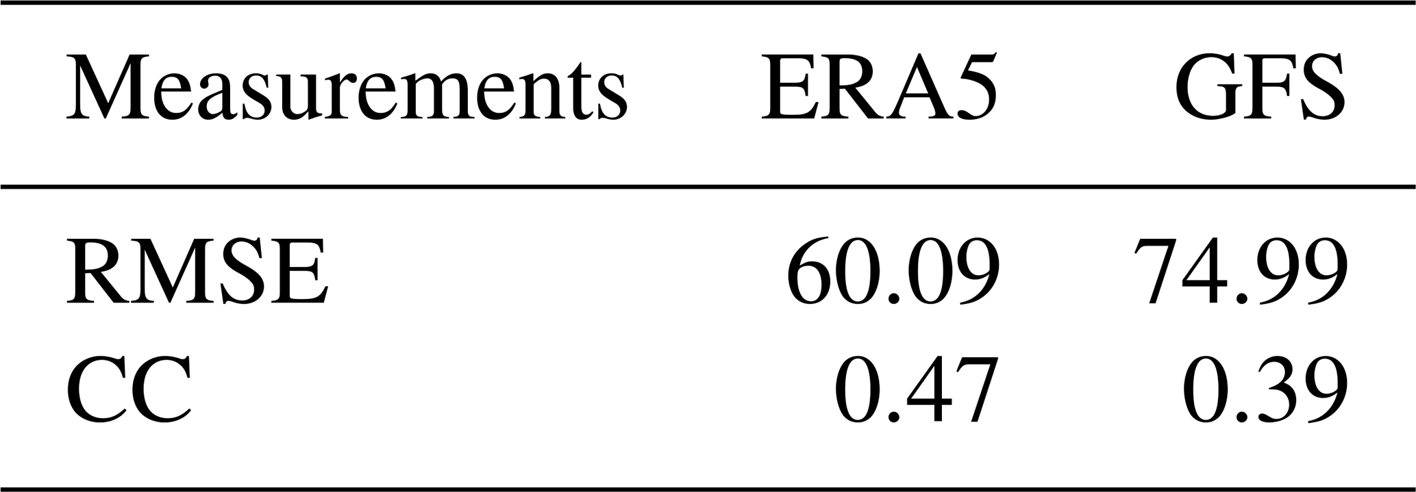
To quantify the differences between simulations and observations, mean root-mean-square errors (RMSEs) and correlations of the 80 grids during the whole event (from 00:00 BJT on 30 November to 00:00 BJT on 4 December 2017) are calculated against the observations. As shown in Table 1, the mean RMSE of the simulations initialized by ERA5 is 60.09 µg m−3 for the PM2.5 concentration, which is 19.87 % lower than that of the GFS simulations (i.e. 74.99 µg m−3). The correlation between the ERA5 simulation and the observation is 0.47, which is 20.51 % higher than the correlation between the observation and GFS simulation (i.e. 0.39). More specifically, we select two time points to show the PM2.5 differences between simulations and observations, which are at 02:00 BJT on 2 December (hereafter defined as accumulation time; AT) and 14:00 BJT on 3 December (hereafter defined as dissipation time; DT). Almost all GFS simulations show an underestimation of the PM2.5 at the AT and an overestimation at the DT. The mean deviations are −47.88 µg m−3 at the AT and 55.02 µg m−3 at the DT. The ERA5 simulation performs much better at the two time points, with mean deviations of −30.57 and 41.58 µg m−3, respectively, although it also shows an underestimation at the AT and an overestimation at the DT.
Table 1The RMSE (µg m−3) and correlation coefficient (CC) of PM2.5 concentrations between simulations initialized by ERA5 and GFS and observations averaged over 80 stations.
It is known that a bad forecast made by a numerical model is attributed to errors in both models and initial conditions. The study of targeted observations aims to improve the forecast by reducing the errors in the initial conditions, which is usually implemented with perfect model assumptions (Mu et al., 2015). A perfect model is assumed to limit forecast errors that result only from errors in the initial conditions, thus simplifying the complexity of problems. However, there are no perfect models in reality. Thus, when implementing the targeted observation tasks, we choose the model that exhibits relatively small model errors and is able to present good simulations to determine where (i.e. the sensitive area) to deploy the targeted observations by calculating the CNOP. The WRF is one of the most advanced weather forecasting models currently and exhibits small model errors (Liu et al., 2012). Therefore, we apply the WRF, together with the NAQPMS model, to explore the role of targeted observations in PM2.5 forecasts. When we use different initial conditions to simulate PM2.5, a better simulation is taken as the “truth run”, and the CNOP is calculated based on that. As shown above, the simulations initialized by ERA5 have better performances in presenting the PM2.5 variability; specifically, they show the best simulation at the AT for the accumulation process of PM2.5 and at the DT for the dissipation process. Thus, the simulations initialized by ERA5, especially at AT and DT, are taken as the truth run to determine the sensitive area for targeted observations by calculating the CNOP, even though the calculated sensitive area is actually an approximation of the real sensitive area. If such approximation is valid, then preferentially assimilating additional observations in the sensitive area will help improve the PM2.5 forecasting skill greatly for any forecast. The validity of the above approximate sensitive area is often tested by prescribing a good simulation to the observations (for example, the simulation initialized by ERA5) and then assimilating the simulated observations located in the sensitive area to a bad forecast (for example, the control forecast) to examine whether the assimilation forecast will be much closer to the good simulation, which is actually a kind of OSSE (see Masutani et al., 2010; Qin et al., 2013). In our study, to verify the validity of the sensitive area, the simulated targeted observations are assimilated to the GFS forecasts to improve their PM2.5 forecasts, where the GFS forecasts are taken as the “control run” and those after assimilating targeted observations are regarded as the “assimilation run”. If the sensitive area is valid, the PM2.5 forecasts in the assimilation run will be much closer to the truth run. It can also be inferred that if the real observations are available, assimilating the real targeted observations to the initial field of the meteorology of the control forecast would improve the PM2.5 forecast skill greatly against the observations. In the present study, we will adopt assimilating simulated observations to verify the validity of the sensitive area due to the lack of available observations.
3.2 CNOP-type errors of meteorological field forecasting
We select the AT and DT as verification times separately to determine the sensitive areas by calculating the CNOP-type errors. When the AT is taken as the verification time, we explore the forecast starting from 02:00 BJT on 1 December, with a lead time of 24 h, and the forecast starting from 14:00 BJT on 1 December, with a lead time of 12 h. When the DT is taken as the verification time, the forecasts starting from 14:00 BJT on 2 December and 02:00 BJT on 3 December, with lead times of 24 and 12 h, respectively, are investigated. Thus, there are a total of four PM2.5 forecasts used here for the heavy haze event that occurred in the BTH region from 30 November to 4 December 2017, and these are all initialized by ERA5.
As we described in Sect. 2.2, the CNOP-type initial errors, which include the variables of wind, temperature, pressure and water vapour mixing ratio, cause the largest forecast error in the studied meteorological fields when measured by the total energy at the verification time in the verification area, which may perturb the PM2.5 forecast to the greatest extent when considering the combined effect of different meteorological components and thus represent the most disturbing initial error in the meteorological field. The CNOP-type errors are calculated separately for these four forecasts. Figures 3–6 plot the horizontal structures of the CNOP-type errors (including wind, temperature and water vapour perturbations) at ground level (approximately 1000 hPa), low-pressure level (approximately 850 and 750 hPa), middle-pressure level (approximately 500 hPa) and upper-pressure level (approximately 200 hPa) for the four forecasts. All wind, temperature and water vapour components of the CNOP-type errors, whether for the AT or DT, are mainly concentrated at ground and low-pressure levels, with large errors lying at the low-pressure levels for a lead time of 24 h and ground level for a lead time of 12 h.
Regarding the CNOP-type errors for the AT, their dominant anomalies, as mentioned above, occur at the low-pressure level (i.e. 850 hPa) for the forecast, with a lead time of 24 h. Furthermore, the horizontal pattern mainly presents two areas that cover the large CNOP-type errors, despite small position differences among the respective large-error areas of wind, temperature and water vapour components at the 850 hPa level (see Fig. 3). One area is near the southern part of the BTH region, with southerly wind bias and positive temperature and water vapour biases, while the other area is in central Mongolia, with southerly wind, positive temperature and negative water vapour biases. However, at ground level, the horizontal patterns present different areas with large errors for the three meteorological components: the wind presents large errors in the southern and western parts of the BTH region, while the temperature and water vapour components present large errors in the western part of the BTH region. For the forecast with a lead time of 12 h, the CNOP-type errors are dominant at ground level but mainly confined to Beijing, with large northerly wind bias and positive temperature and water vapour biases (see Fig. 4). In addition, the wind and water vapour also present large errors in Shandong Province. At the low-pressure level (i.e. 850 hPa), the maximum errors of wind and temperature are located in the northwestern part of the BTH region, near Baotou city, but the maximum error of water vapour is found in Shandong Province in the southeastern part of the BTH region.
When the DT is the verification time, it can be seen that the CNOP-type errors mainly occur at low-pressure levels (i.e. 850 and 750 hPa), for a lead time of 24 h, where a large northerly wind bias and negative temperature and water vapour biases occur in southern Mongolia. Despite their specific positions only having small differences, the location of large water vapour errors is further west than those of the large errors of wind and temperature (see Fig. 5). For a lead time of 12 h, the large northwesterly wind errors are concentrated at the ground level, while the large positive temperature and water vapour errors occur at low-pressure levels. Furthermore, there are also large temperature and water vapour errors occurring at the low- and middle-pressure levels (see Fig. 6).
It is clear that the CNOP-type errors peak at different vertical levels for the four forecasts. For the meteorological fields of wind, temperature and water vapour, even at the same vertical level, the areas with large errors in different variables are somewhat different. The errors in the areas where the CNOP-type errors are concentrated could make the largest contribution to the forecast errors of the verification area at the verification time, and therefore they can be regarded as a sensitive area for targeted observations associated with PM2.5 forecasts. However, from the above CNOP-type errors, it is known that such areas are dependent on different meteorological variables and are located at different vertical levels and regions, which makes it unclear which meteorological variables, levels and areas should be identified for preferential treatment and provides challenges to real field campaigns. Thus, in this situation, how do we address the problems related to targeted observations for the meteorological fields associated with PM2.5 forecasting? We will address this question in the next section.
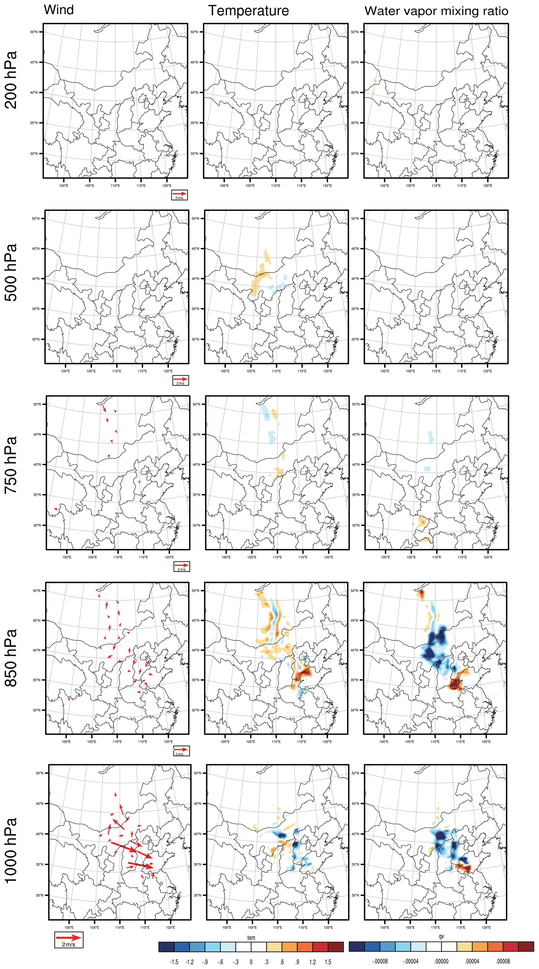
Figure 3The horizontal distribution of the CNOP-type errors, including the wind component (vector, left column, m s−1), temperature component (shaded, middle column, ∘) and water vapour mixing ratio component (shaded, right column, kg kg−1) at an upper-pressure level (approximately 200 hPa), middle-pressure level (approximately 500 hPa), low-pressure level (approximately 850 hPa) and ground level (approximately 1000 hPa) for the forecast starting from 02:00 BJT on 1 December, with a lead time of 24 h.
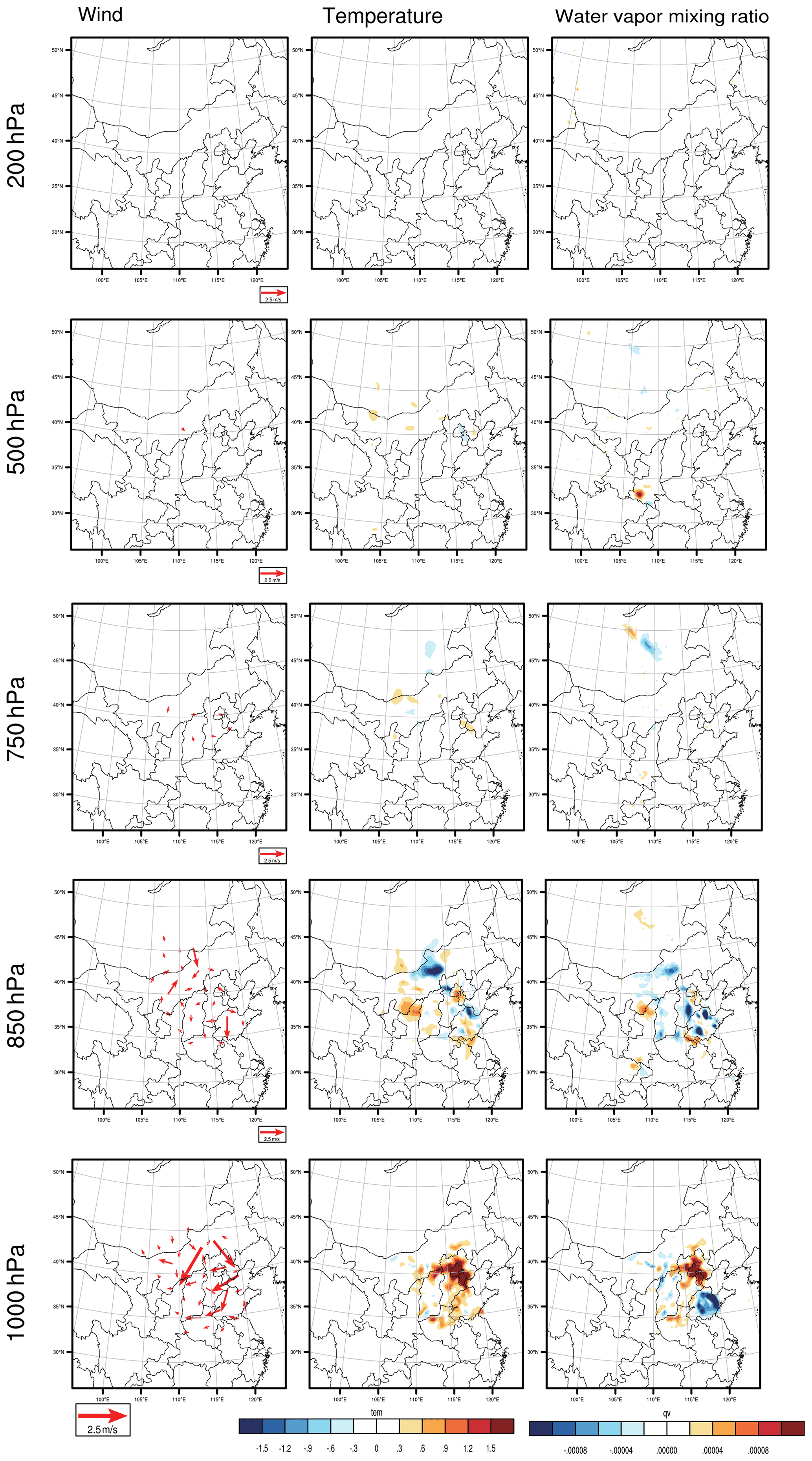
Figure 4The same as in Fig. 3 but for the forecast starting from 14:00 BJT on 1 December, with a lead time of 12 h.

Figure 5The same as in Fig. 3 but for the forecast starting from 14:00 BJT on 2 December, with a lead time of 24 h.

Figure 6The same as in Fig. 3 but for the forecast starting from 02:00 BJT on 3 December, with a lead time of 12 h.
In this section, we propose an approach to measure the comprehensive sensitivity of initial errors occurring in different vertical levels and horizontal areas for different meteorological variables. Following this, the sensitive areas for targeted observations can be identified by this comprehensive sensitivity that considers the information of all meteorological variables at all pressure levels.
4.1 The sensitive areas for targeted observations associated with PM2.5 forecasts
To evaluate the comprehensive sensitivity of the CNOP-type initial errors occurring at different vertical levels and areas for different meteorological fields, a vertical integral (VI) of the CNOP-type errors, as shown in Eq. (4), is calculated.
The VI consists of all concerned meteorological variables and their vertical distributions and measures the comprehensive sensitivity of forecasting uncertainties on initial errors of different meteorological variables. In this situation, the PM2.5 forecast could be very sensitive to the combined effect of initial errors of the meteorological fields in the area of a larger VI, and preferentially reducing the meteorological initial errors in these sensitive areas will lead to much larger improvements of the meteorological forecasts over the BTH region, which then significantly improves the regional PM2.5 forecasts.
Figure 7 shows the horizontal distribution of the VI for the four forecasts. When the AT is the verification time, two areas are identified to have large VIs for the forecast starting from 02:00 BJT on 1 December, with a lead time of 24 h. One area is near Dezhou, which lies to the southeast of Hebei Province, and the other area is located in central Inner Mongolia and extends to Mongolia. We regard these two areas as the sensitive areas for meteorological field forecasting, and we then regard the PM2.5 forecast of the BTH region at the AT, with a lead time of 24 h. Similarly, we identify the sensitive area for the forecast with a lead time of 12 h in Beijing and Tianjin. For the verification time DT, the sensitive areas are determined as the region from Hohhot in Inner Mongolia to the Altai Mountains in Mongolia for a lead time of 24 h. For a lead time of 12 h, the sensitive areas are mainly located in Zhangjiakou and Chengde, which lie in the northern part of the BTH region.
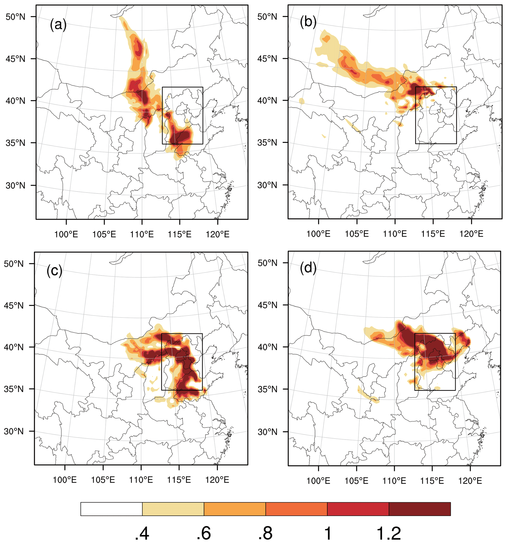
Figure 7The horizontal distribution of the VI (J kg−1) for the forecasts at the AT with lead times of (a) 24 h and (c) 12 h and for the forecasts at the DT with lead times of (b) 24 h and (d) 12 h. The black rectangle is the verification area.
4.2 Validity of targeted observations in improving PM2.5- forecasting skill
According to the definition of targeted observations, deploying additional observations in the sensitive areas and assimilating them to the initial field will improve the forecasting skill of the meteorological field and then the PM2.5. If such improvement is significantly larger than those of assimilating the additional observations in other areas, the sensitivity of the targeted observations in the sensitive area determined by the CNOP is confirmed numerically. With the above argument, the better simulation of PM2.5 with the meteorological field forecast by ERA5 is assumed to be the truth run, and thus the worse simulation initialized by the GFS is the control run (see Sect. 3.1); thus, the differences between the PM2.5 concentrations in the control and truth runs can be regarded as forecast errors of the control run with respect to the truth run. Figure 8 shows the spatial distributions of forecast errors of PM2.5 at the AT and DT. This shows that the control run has an obvious underestimation of the PM2.5 concentrations over the whole BTH region at the AT and an overestimation at the DT. If taking the absolute value of the biases, then the mean biases of the whole BTH region are 34.22 and 64.13 µg m−3 at the AT and DT, respectively. To verify the validity of the targeted observations in the sensitive areas, we take relevant meteorological fields in the truth run but confine them to the identified sensitive areas as “additional observations” (i.e. artificial targeted observations) and assimilate them to the initial fields of the control run by the 3D-Var assimilation system of the WRF (see Sect. 2.1), finally obtaining an updated forecast of the PM2.5 concentration, which, as defined in Sect. 3.1, is called the assimilation run. The validity of targeted observations for improving PM2.5 forecasts of the control run is quantified by two indices defined by Eqs. (5) and (6),
where AEV and AEM are the percent change of the forecast errors at verification times (see Eq. 5) and that during the whole forecast period (see Eq. 6) after assimilating the control forecast, respectively, and PC, PT and PA denote the PM2.5 concentration in the control run, truth run and assimilation run, respectively. The sign |•| measures the amplitude of forecast errors averaged over the BTH region, T represents the verification time and t0 is the initial time of the forecast. A positive value of AEV and AEM indicates an improvement in forecast skills, and the larger the positive values are, the more significant the improvements. A negative value of AEV and AEM indicates a decline in forecast skills.
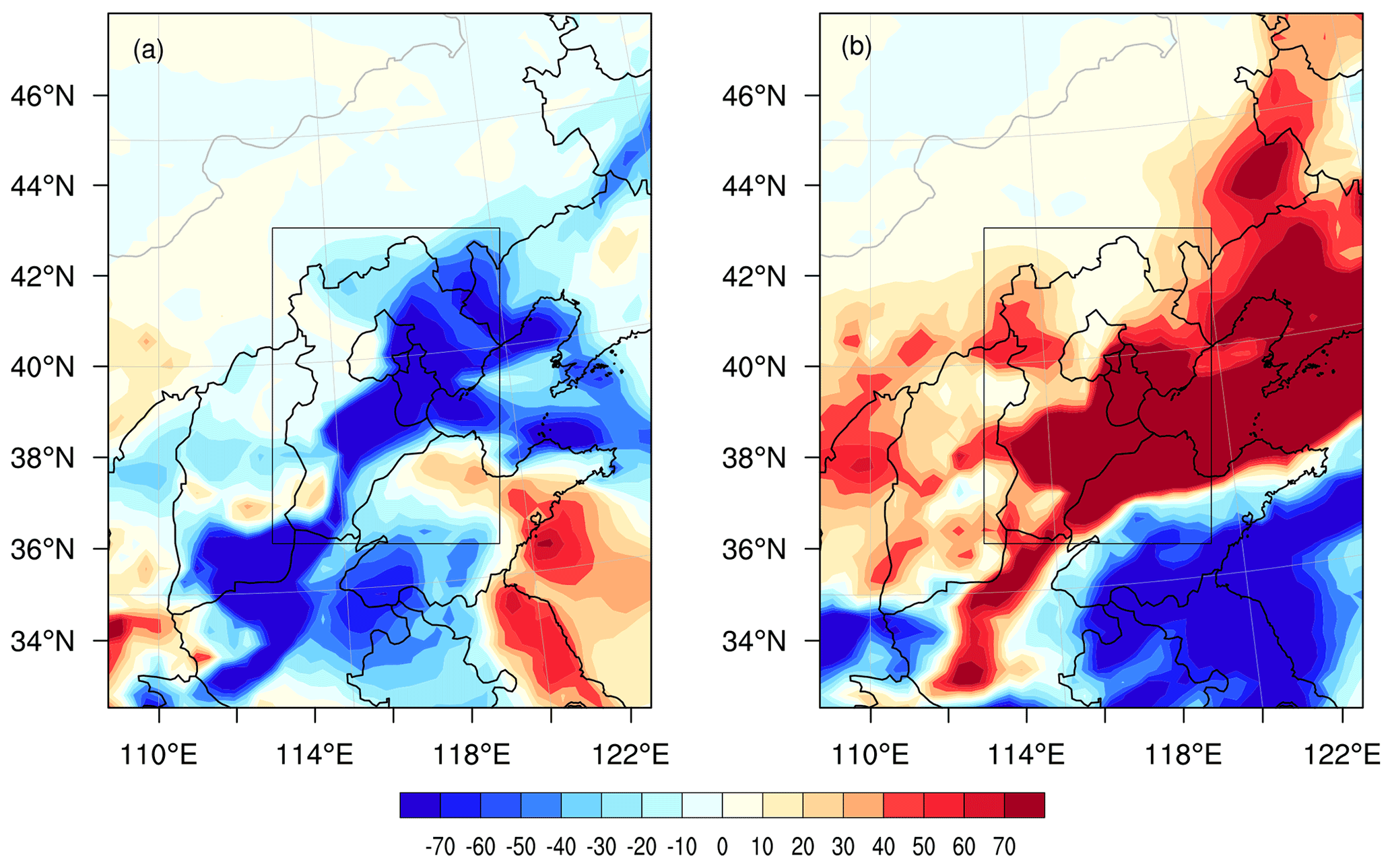
Figure 8The spatial distributions of PM2.5 forecast errors (µg m3) in the control run at the (a) AT and (b) DT. The black rectangle is the verification area.
We take the artificial additional observations of meteorological fields located at a fixed number of 15 horizonal observation positions, which are located through the vertical 950, 850, 750 and 500 hPa levels (60 observations at the four pressure levels in total) and include horizontal wind, temperature and relative humidity. These observation positions are considered to be covered by the sensitive areas identified by the VI of the CNOP-type errors. To determine the optimal observation array in the sensitive areas, additional observations are experimentally distributed every 30, 60, 90, 120 and 150 km. Specifically, we take the observation distance of 150 km as an example. The grid point with the largest VI is taken as the first observation position. Following this, we exclude the grids that are no further than 150 km away from the first observation position and determine one of the largest VIs among the remaining grids as the second observation position. After the second observation position is fixed, we exclude the grids that are no further than 150 km away from the second observation position, and the grid of the largest VI among the remaining grids is determined as the third observation position. The other 12 observation positions can be similarly determined. Note that the fixed number of the observation positions (15) is experimentally selected, and one can choose other numbers to conduct experiments. In accordance with the above approach, we can obtain 5 observation arrays with 15 predetermined observation positions.
By assimilating the five observation arrays to the initial fields of control runs, new forecasts (i.e. the assimilation runs) of PM2.5 are obtained. The improvements in the forecasting skill against the truth runs are shown in Tables 2 and 3. For a 24 h lead time of the forecast at the AT, assimilating the five observation arrays can improve the PM2.5 forecast skill by reducing the forecast errors ranging from 4.29 to 6.91 µg m−3, accounting for 12.54 % to 20.20 % of the forecast errors in control runs measured by AEV at the AT; the mean forecast errors during the whole forecast period can decrease from 19.79 % to 29.20 % measured by AEM (from exactly 3.58 to 5.28 µg m−3) (Table 2). Of the five observation arrays, the array with observation positions every 90 km shows the largest improvement measured by AEV and AEM. When the 15 observation positions are deployed every 90 km, approximately 68 % of the grids over the BTH region show positive AEV values, and the largest improvement in PM2.5 forecasts reaches 73.80 µg m−3, located in Cangzhou in southeastern Hebei Province (Fig. 9a). When the observation arrays are deployed 12 h before the AT, a larger improvement in forecasting skills can be found (Table 2). Of the five observation arrays, the improvements in forecasting skills at the AT measured by AEV range from 24.53 % to 43.26 %, and the mean improvement during the whole forecast period measured by the AEM ranges from 32.84 % to 50.81 %, where the observation array deployed at a distance of 150 km shows the largest improvements in terms of both AEV and AEM despite the observations being relatively sparse in this array. Overall, the observations deployed 12 h before the AT in the sensitive areas identified by the CNOP-type errors measured by the VI show better performances than those deployed 24 h before the AT. Thus, if we care about improving the PM2.5 forecast at the AT and the number of observation positions is fixed at 15 (only accounting for 0.17 % of the grids over the domain), the observation array with an observation position distance of 150 km deployed in the sensitive areas (i.e. locations in Beijing and Tianjin) at 12 h before the AT might be the optimal choice for targeted observations; in this case, the forecast error of PM2.5 could decrease by as much as 43.26 % at the AT in terms of the AEV and 50.81 % during the whole forecast period in terms of the AEM (see also Table 2).
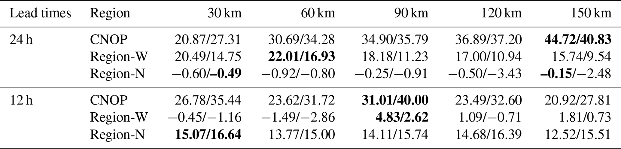
Table 2The AEV AEM of the forecasts at the AT, with lead times of 24 and 12 h, when the additional observations in the sensitive region (CNOP), Region-W and Region-N are assimilated (%). The respective optimal observation array is marked in bold.
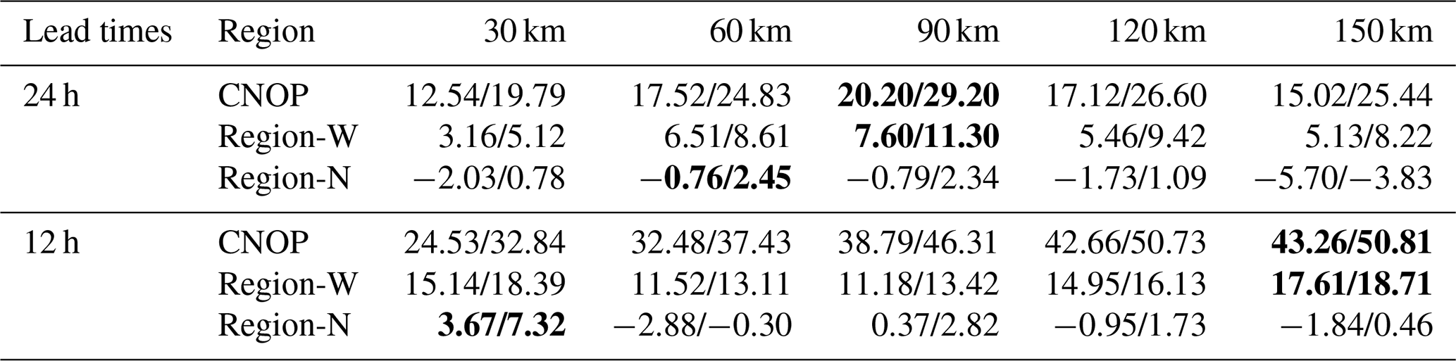
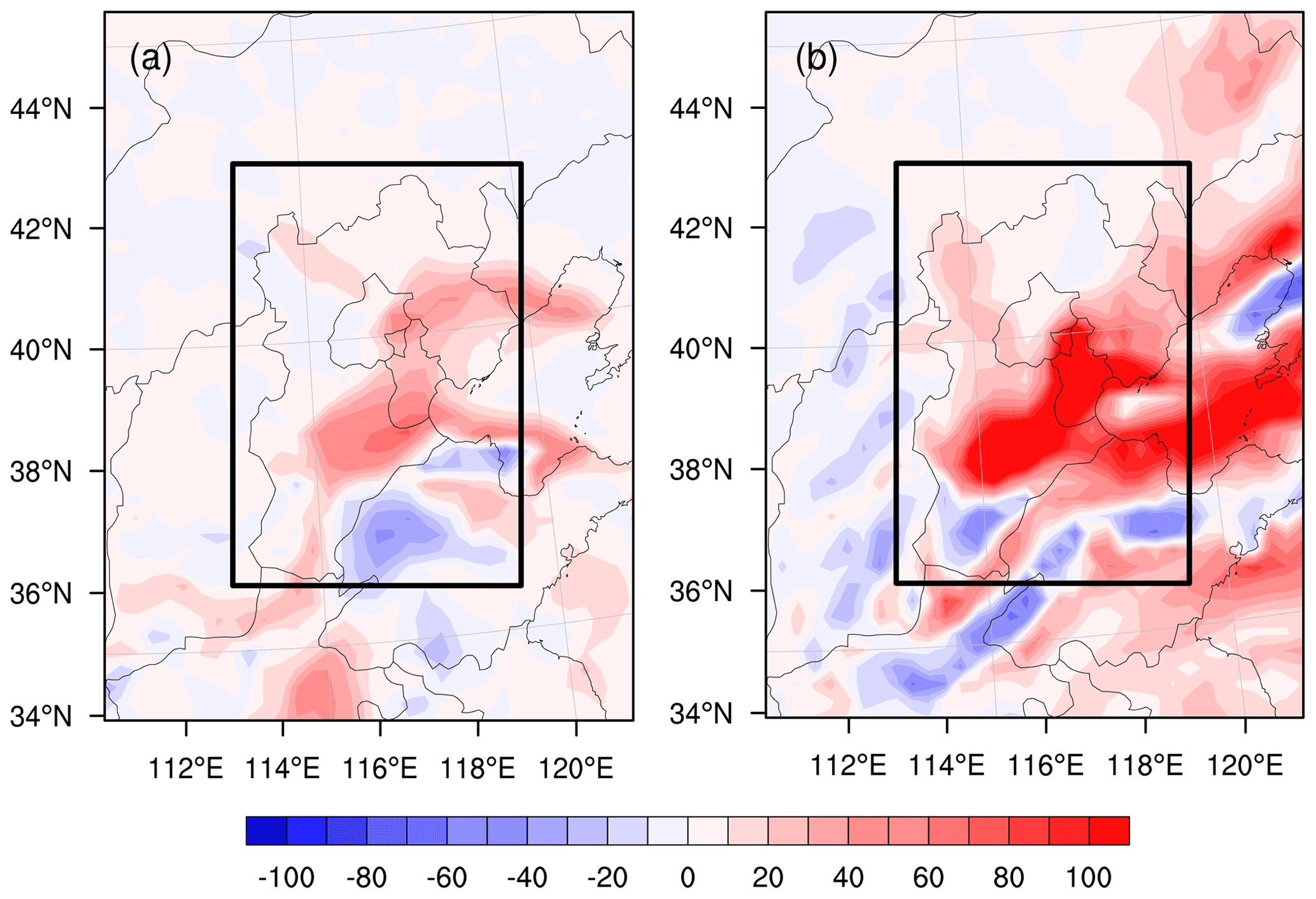
Figure 9The spatial distributions of the improvement in PM2.5 forecasts (µg m3) at the (a) AT and (b) DT, with a lead time of 24 h. The black rectangle is the verification area.
To improve the PM2.5 forecast at the DT, five observation arrays in the corresponding sensitive areas can be similarly obtained, and of these arrays, their assimilation runs improve the PM2.5 forecast skills, with the AEV varying from 20.87 % to 44.72 % (from exactly 13.39 to 28.77 µg m−3) and AEM from 27.31 % to 40.83 % (from exactly 8.27 to 11.90 µg m−3; Table 3) for a lead time of 24 h. The assimilation run with the observation array of the observation positions every 150 km shows the largest improvement in both AEV and AEM. Specifically, when the observation arrays are deployed every 150 km, an area of approximately 81 % of the grids over the BTH region shows positive AEV values, and the largest improvement in the PM2.5 forecast, reaching 202.64 µg m−3, occurs in Tianjin (Fig. 9b). However, when the lead time is reduced to 12 h, the mean improvements are less than the forecast with a lead time of 24 h, with the AEV varying from 20.92 % to 31.01 % (from exactly 11.24 to 16.66 µg m−3) and AEM from 27.81 % to 40.00 % (from exactly 6.95 to 10.00 µg m−3, Table 3). Among the five observation arrays, the observations with an observation position distance of 90 km show the largest improvement in both AEV and AEM, which is different from the optimal observation array of observation positions every 150 km deployed 24 h before the DT. In contrast, the last array has the worst performance. Overall, if we care about improving the PM2.5 forecast skills at the DT, the optimal observation arrays should be deployed over the sensitive areas (i.e. locations in Mongolia) with an observation position distance of 150 km at 24 h before the DT, and assimilating the observations could reduce the forecast errors by as much as 44.72 % at the DT measured by AEV and 40.83 % during the forecast period measured by the AEM. All of these results are also summarized in Table 3.
Through a series of OSSEs, the effectiveness of targeted observation is conducted by deploying a fixed number of observations (15 horizonal grids through 4 pressure levels), and observations deployed at different distances are evaluated to determine the optimal observation array. The results show that when the observation number is fixed, an appropriate observing distance (not necessarily a large observing distance) is essential to obtain the largest improvement in PM2.5 forecast skills. To further examine the role of appropriate observing distance, we also conducted the following experiments that observations are deployed within a limited area with different observing distances (which corresponds to different observation numbers in the limited area). Specifically, we first select a the 120 most sensitive grids to define the sensitive area in each of the four forecasts according to the VI value. Within the given size of the sensitive area, the observing arrays with a distance of 30, 60, 90, 120 and 150 km are determined using the same method as the experiments described above. The additional observations are assimilated to the control run, and the improvements of PM2.5 forecast skills are shown in Fig. 10. For the two forecasts at the AT and the forecast at the DT with a lead time of 24 h, the observation arrays with a distance of 30 km show the largest improvement in both AEV and AEM. This implies that in the given sensitive area size, denser observation sites can better resolve the synoptic initial conditions within the sensitive area, which in turn enhance the forecasting skills more effectively. However, for the forecast at the DT with a lead time of 12 h, the observations with the distance of 90 km show the largest improvement. This implies that in this forecast it is not necessarily the use of much denser observation locations but instead the choice of an appropriate location that is most important for improving the PM2.5 forecasts. Thus, here we emphasize that the observations deployed at a large distance or a high density will not necessarily result in the largest improvement in PM2.5 forecast skills. This suggests that the observations should be deployed carefully with an appropriate distance to get the largest benefits when implementing the field campaigns.
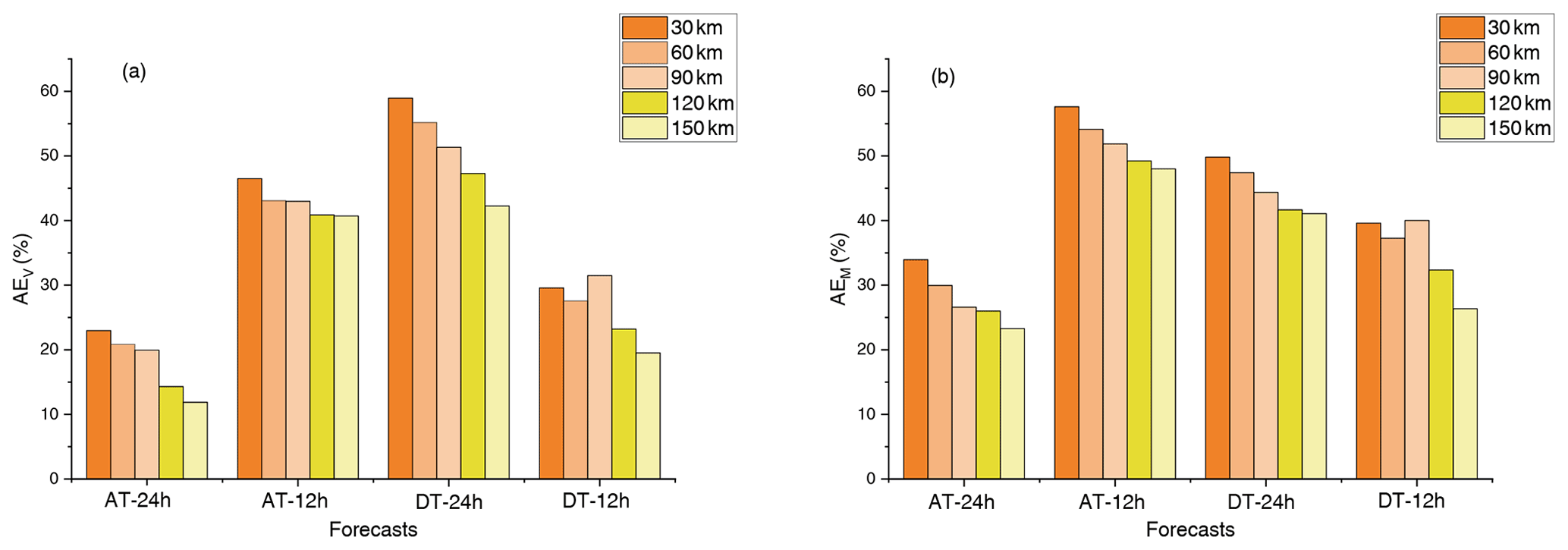
Figure 10The bar plots of (a) AEV and (b) AEM values of the four forecasts, when the additional observations are deployed within a limited size of area with different observing distances.
4.3 A comparison between targeted observations and other additional observations in improving PM2.5 forecasts
The results in Sect. 3.2 show that assimilating targeted observations in the sensitive areas determined by the CNOP-type errors can largely improve the PM2.5 forecasting skills (hereafter referred to as CNOP-EXPs). To further illustrate the usefulness of CNOP in identifying the sensitive area for targeted observations, here we compare the sensitive areas and other areas surrounding the BTH region.
Apart from the sensitive areas identified by CNOP-type errors, other areas surrounding the BTH region are mainly located in the southwestern, southeastern, eastern and northern parts of the BTH region. Previous studies demonstrated that the PM2.5 concentrations in the BTH region are continuously influenced by weather conditions (especially wind anomalies) in the southwestern and northern parts of the BTH region (Sun et al., 2019; Zhang et al., 2018). Specifically, they showed that southwesterly wind anomalies tend to transport the polluted air from the southwestern part of the BTH region and that northerly wind anomalies blow away BTH pollution. It therefore seems that the PM2.5 forecasts are more sensitive to the meteorological conditions along the southwestern (i.e. Shanxi Province) and northern (i.e. Inner Mongolia) directions of the BTH region. To examine this sensitivity, we select two areas in these two directions that are similar to the sensitive areas identified by the CNOP-type errors and surround the BTH region. Specifically, we refer to these two areas as Region-W (29.5–36.0∘ N, 100.5–113.5∘ E) and Region-N (42.5–51.0∘ N, 115.5–126.0∘ E), whose area sizes are approximately the same as those of the sensitive areas identified by the CNOP-type errors. In each region, we calculate the initial errors of meteorological conditions that lead to the largest forecast error at the verification time in the BTH region, which represent the most sensitive initial errors in this area to PM2.5 forecasts. The algorithms are the same as those used for calculating the CNOP-type errors, but the initial perturbations are restricted to only Region-W and Region-N. We also use the vertical integral of the errors (VI) to determine the observation arrays and evaluate the sensitivity of PM2.5 forecasting uncertainties to the meteorological initial errors over these two regions. Specifically, the observation arrays in these two areas are constructed with the same configuration as in the area identified by CNOP-type errors. Following this, five observation arrays are similarly obtained for Region-W and Region-N. Two groups of experiments are implemented separately for the aforementioned four forecasts, i.e. the forecasts aimed at the AT with lead times of 12 and 24 h and those aimed at DT with lead times of 12 and 24 h.
The results are shown in Tables 2 and 3. For the 24 h lead time forecast at the AT, the five observation arrays in Region-W are assimilated, and they can improve the PM2.5 forecast skill of the BTH region, with improved AEV and AEM ranging from 3.16 % to 7.60 % 5.12 % to 11.30 %, respectively (see Table 2). These improvements measured by AEV and AEM are approximately one-third of those in CNOP-EXPs on average for the five observation array assimilations, with the former being 5.57 % and 16.48 % and the latter being 8.53 % and 25.17 % for AEV and AEM, respectively. Although the observation array with a distance of 90 km has the best performance for the improvements in the PM2.5 forecasts in Region-W, this improvement is still lower than that of the worst example among the forecasts with the five observation arrays in CNOP-EXPs. When the five observation arrays are deployed over Region-N and assimilated to forecast the PM2.5 in the control run, the AEV values at the AT are all negative for a lead time of 24 h, which indicates a decline in the forecasting skills for the PM2.5 at the AT compared with the control run, regardless of which observation array is assimilated. For the mean of the forecast skill during the whole forecast period (as measured by AEM), the observation array with an adjacent distance of 150 km presents a negative value of AEM when it is assimilated to forecast PM2.5, while the other four observation arrays present a positive value of AEM, but with a mean improvement of only 1.67 %, far less than the 25.17 % seen in CNOP-EXPs. It is reasonable that assimilating observations in the Region-N may result in a worse forecast. Theoretically, if the observations in the area where the forecast is not sensitive to the initial values are assimilated, the forecasting skills will be improved slightly or will remain neutral. However, when implementing the realistic prediction, the imperfect procedure of data assimilation, the observation errors, model errors, the unresolved scales and processes in the model, and other combined effects may induce additional errors (Janjić et al., 2018), which may be the reason that assimilating observations in the unsensitive area results in a worse forecast. That also indicates that Region-N is not the sensitive area for the forecast at the AT. For the 12 h lead time PM2.5 forecast at the AT, we also show that the five observation arrays in Region-W and Region-N present far fewer improvements in PM2.5 forecast skills than those in CNOP-EXPs when they are assimilated to forecast PM2.5 (see Table 2). Specifically, the improvements measured by the AEV and averaged for the five observation arrays in Region-W and Region-N (i.e. 14.08 % and −0.33 %, respectively) are approximately and of that (i.e. 36.34 %) in CNOP-EXPs, and the improvements measured by AEM (i.e. 15.92 % and 2.41 %, respectively) are approximately and of that (i.e. 43.62 %) in CNOP-EXPs, respectively. From the above experiments, it is obvious that for the 24 and 12 h lead time forecasts at the AT, the five observation arrays deployed in Region-W and Region-N, although they often enhance the forecast skill of PM2.5 against the control run, present improvements in the PM2.5 forecast skill that are significantly smaller than those in the CNOP-EXPs. This shows that the sensitive areas for targeted observations of meteorological fields associated with the PM2.5 forecast at the AT are most likely to be the ones identified by the CNOP-type errors, rather than those at Region-W and Region-N.
For the PM2.5 forecasts at the DT, the results also illustrate the strong sensitivity of the targeted observations in the sensitive area identified by the CNOP-type errors. Specifically, for the 24 h lead time forecast, the observation arrays in Region-W tend to benefit the PM2.5 forecast, and the improvement averaged for five observation arrays is 18.68 % for the AEV and 12.68 % for the AEM, which are both nearly half of those in the CNOP-EXPs. When the five observation arrays are deployed in Region-N, they all lead to worse forecasts at the DT than the control run, with the AEV varying from −0.92 % to −0.15 % and the AEM from −3.43 % to −0.49 % (Table 3). For the 12 h lead time forecasts, the five observation arrays deployed in Region-W do not significantly improve the PM2.5 forecast, with AEV values ranging from −0.45 % to 4.83 % and AEM values from −2.86 % to 2.62 %; in contrast, the five observation arrays deployed in Region-N considerably improve the PM2.5 forecasts, with AEV ranging from 12.52 % to 15.07 % and AEM from 15.00 % to 16.64 %, where the observation array with an adjacent distance of 30 km shows the best performance of the five observation arrays for improving the PM2.5 forecast skill. Despite this, the improvement is still less than that of the worst forecast in CNOP-EXPs, where the observation array was at an adjacent distance of 150 km. Specifically, the improvements in AEV and AEM are 14.03 % and 15.85 %, respectively, which are both averaged for five observation arrays and approximately 50 % lower than those in CNOP-EXPs. Therefore, the sensitive areas for targeted observation of meteorological fields associated with the PM2.5 forecast at the DT are the ones identified by the CNOP-type errors, i.e. the area from Hohhot in Inner Mongolia to the Altai Mountains in Mongolia (for a lead time of 24 h) and the area from Zhangjiakou and Chengde in the northern part of the BTH region (for a lead time of 12 h).
In this section, we further interpret why the sensitive area identified by CNOP-type errors can result in a larger improvement in PM2.5 forecast skill. It is known that dynamic and thermodynamic conditions are two key factors that determine the transport and deposition of pollution. With a relatively strong wind, pollution can be transported to the downwind region in a short time, while a relatively calm wind could favour ground pollution accumulation. For the BTH region, northerly winds blow away PM2.5, while southerly winds lead to the accumulation of PM2.5 through the blocking effect of the surrounding mountains (Zhao et al., 2009). Thermodynamic conditions such as the strong temperature inversions in the atmospheric boundary layer are also favourable for the accumulation of air pollutants to form air pollution events (Miao et al., 2015). Moreover, an increased temperature may accelerate the production rate of precursors and secondary pollutants, which contribute to variations in ground-level PM2.5.
In this paper, we showed that the control run with a lead time of either 12 h or 24 h presents a severe underestimation of PM2.5 at the AT and a large overestimation of PM2.5 at the DT for the heavy air pollution event that occurred from 30 November to 4 December 2017 (see Sect. 3.1). The assimilation runs greatly improve the skill of these PM2.5 forecasts by assimilating the targeted observations in the sensitive areas of the meteorological fields. Here, we interpret why the assimilation runs increase the PM2.5 forecast skill for dynamic and thermodynamic reasons. After we compare the forecast biases of the control run with lead times of 12 and 24 h, we find that the forecast biases of the control run under the two leading times are almost the same. For simplicity, we present the forecast with a lead time of 24 h. Figure 11 shows the differences in the wind and temperature fields between the truth run and control run at ground level at the AT and DT, with a lead time of 24 h. The truth run presents significant southerly winds with a mean speed of 2.32 m s−1 over the BTH region (see Fig. 11a), while the control run forecasts a southerly wind with a mean speed of 0.74 m s−1 (see Fig. 11b) and exhibits northerly wind biases, as shown in Fig. 11c. The weak southerly wind in the control run reduces the pollution transported from the south to the BTH region in the truth run, which results in a significant underestimation of the PM2.5 concentration of the control run at the AT. In addition to this dynamic reason, the thermodynamical conditions are also key factors influencing the PM2.5 forecasts. Both the truth run and the control run are able to simulate the temperature inversion layer, which prevents vertical dispersion of pollutants and promotes the accumulation of surface PM2.5. For the forecasts at the AT, the truth run has forecasted 0.11 K 100 m−1 vertical temperature inversion layers at Dongsi station in Beijing, while the control run has forecasted 0.05 K 100 m−1. The mean lapse rate simulated by the truth run over the BTH region is 0.03 K 100 m−1, and the control run has forecasted a rate of 0.002 K 100 m−1. This means that the truth run simulated a more stable thermodynamic condition, which is favourable for the accumulation of surface air pollutants. Meanwhile, the negative temperature bias in the near surface of the control run decreases the production rate of precursors of PM2.5, and the negative bias of relative humidity reduces the useful carrier of PM2.5, causing a decrease in PM2.5, favouring the underestimation of PM2.5 at the AT in the control run.
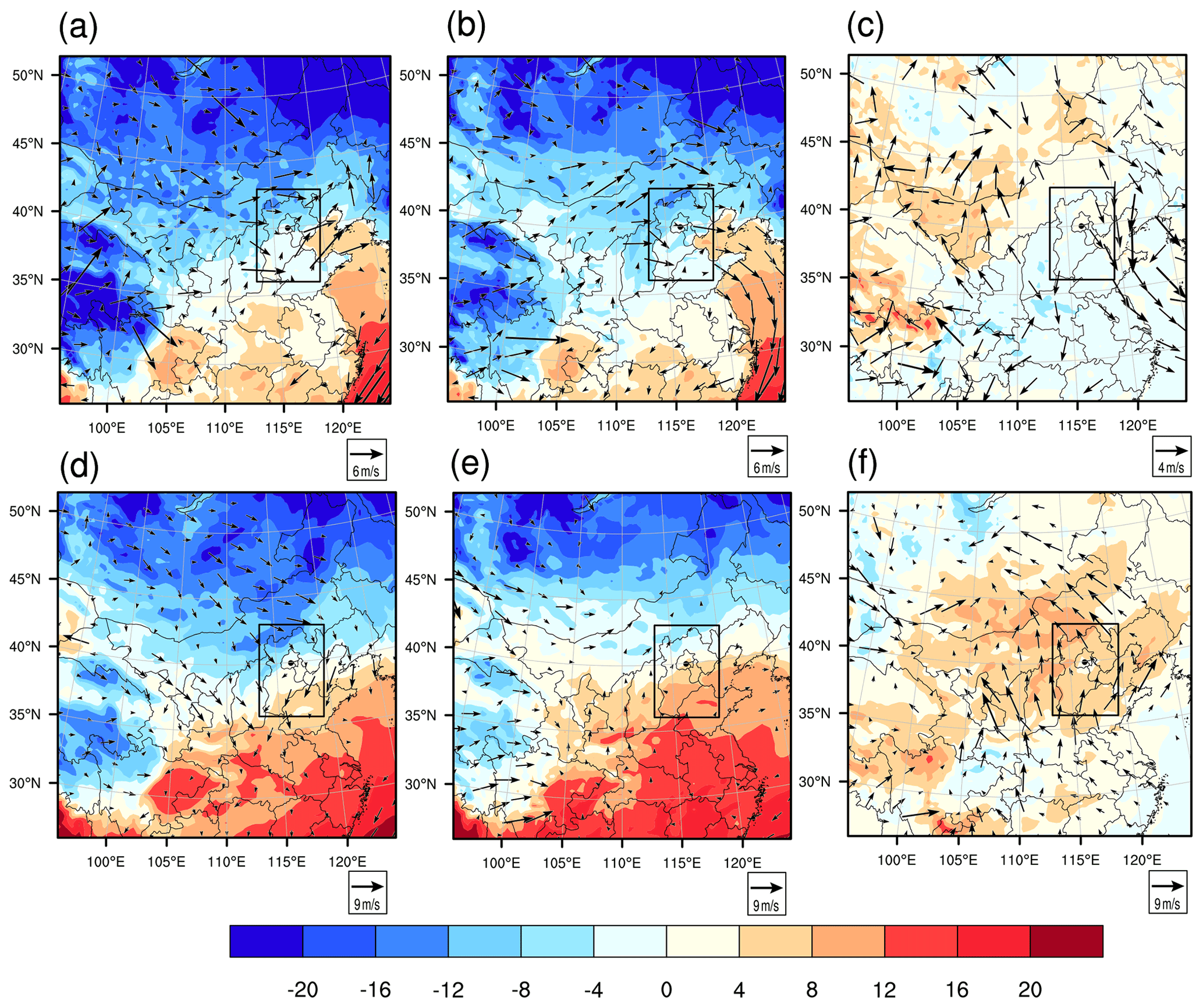
Figure 11The wind (vector, m s−1) and temperature field (shaded, ∘) forecasts at the ground level at the AT (with a lead time of 24 h) of the (a) truth run and (b) control run. The differences in the wind and temperature fields between the truth run and control run (control run minus truth run) at the AT are shown in (c). Panels (d–e) are the same as panels (a–c) but for the forests at the DT.
From the above information, it is clear that the control run exhibits northerly wind, a less stable boundary layer, and low temperature and relative humidity biases at the AT relative to the truth run. However, after assimilating the artificial meteorological variables over the sensitive areas determined by the CNOP-type errors into the initial analysis field of the control run, the PM2.5 forecasts are improved in terms of forecasting skill. For the forecasts with lead times of 12 and 24 h, the interpretations as to why the assimilation runs increase the PM2.5 forecast skill and its related mechanisms are similar. For simplicity, we present the interpretations in detail for the forecast with a lead time of 24 h. In Fig. 12, we plot the spatial evolution of the 24 h forecast differences of wind and PM2.5 concentrations between the CNOP-EXP and control run. From Fig. 12, we can see that the sensitive areas for the PM2.5 forecast at the AT are mainly located in the southern and northwestern parts of the BTH region (also see Fig. 7), and assimilating meteorological observations over the sensitive areas increases the southerly wind in the southern part of the BTH region at the initial field and enhances the southerly wind by 0.18 m s−1 over the BTH region at the verification time, which is helpful for transporting southern pollution to the BTH region. Between the two areas, the sensitive area near Inner Mongolia plays a more dominant role in the PM2.5 forecast of BTH region by inducing a larger southerly wind component. In addition, the assimilation run has forecasted 0.06 K 100 m−1 temperature inversion layers at Dongsi station, and the mean lapse rate over the BTH region has reached 0.004 K 100 m−1. The slightly improved thermodynamic conditions further result in modifications of the boundary layer structure, including a decreased planetary boundary layer height. The mean boundary layer height over the BTH region decreased from 261 m in the control run to 256 m in the assimilation run, which also contributed to the increased ground level PM2.5 pollution and improved the PM2.5 forecast skill in the assimilation run. Moreover, assimilating the targeted observations increases the initial temperature and relative humidity in the western parts of the BTH region and decreases them in the northwestern parts of the BTH region. Following this, the western warm air and northwestern cool air move east and southeast, respectively, which finally decreases the temperature by 0.05 ∘C and the relative humidity by 0.6 % at the AT over the BTH region. Decreased temperature and relative humidity are not beneficial for the formation of PM2.5. From the above analysis, it can be found that the improvements in the PM2.5 forecast skill in assimilation runs result from the increased southerly wind and more stable boundary layer during the accumulation process.
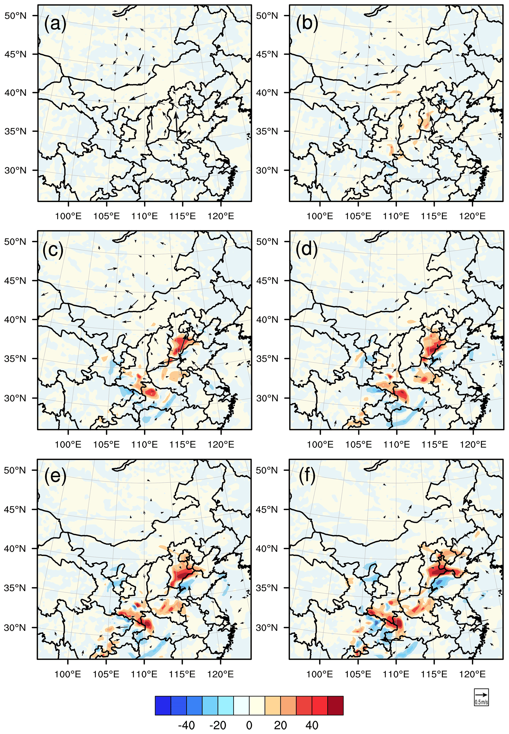
Figure 12The spatial evolution of the forecast differences of ground wind (vector, m s−1) and PM2.5 concentrations (shaded, µg m−3) between the assimilation run (CNOP-EXP with an observing distance of 90 km) and the control run starting from 02:00 BJT 1 December, with lead times of (a) 1 h, (b) 6 h, (c) 11 h, (d) 16 h, (e) 21 h and (f) 24 h.
For the forecast at the DT, the truth run presents a large northerly wind with a mean speed of 5.24 m s−1, as shown in Fig. 11d, which blows the pollution from the BTH region to the south. However, the control run forecasts a southerly wind with a mean speed of 1.82 m s−1 (Fig. 11e), which is the reverse of the truth run and might transport more pollution from the southwestern part to the BTH region than from the BTH region to the south in the truth run, finally contributing to the overestimation of the PM2.5 concentration in the control run. Meanwhile, the control run also presents a warm temperature and much higher relative humidity biases, which prevent the dissipation of PM2.5 over the BTH region and favour the overestimation of PM2.5 at the DT (see Fig. 11f). When the targeted observations are assimilated into the control run at 24 h before the DT and then the assimilation run is formulated, the northerly wind increases and the temperature and relative humidity decrease in the sensitive areas at the initial time, which subsequently drives a large amount of cool and dry air in the sensitive area (i.e. the northwestern part of the BTH region; also shown in Fig. 7) to the south that accumulates over the BTH region (see Fig. 13), decreasing the temperature and relative humidity over the BTH region at the verification time and improving the forecasts of the PM2.5 concentrations in the assimilation run at the DT. It is obvious that the improvement of both the dynamic and thermodynamic conditions is responsible for the increase in the PM2.5 forecast skill at the DT in the assimilation run.
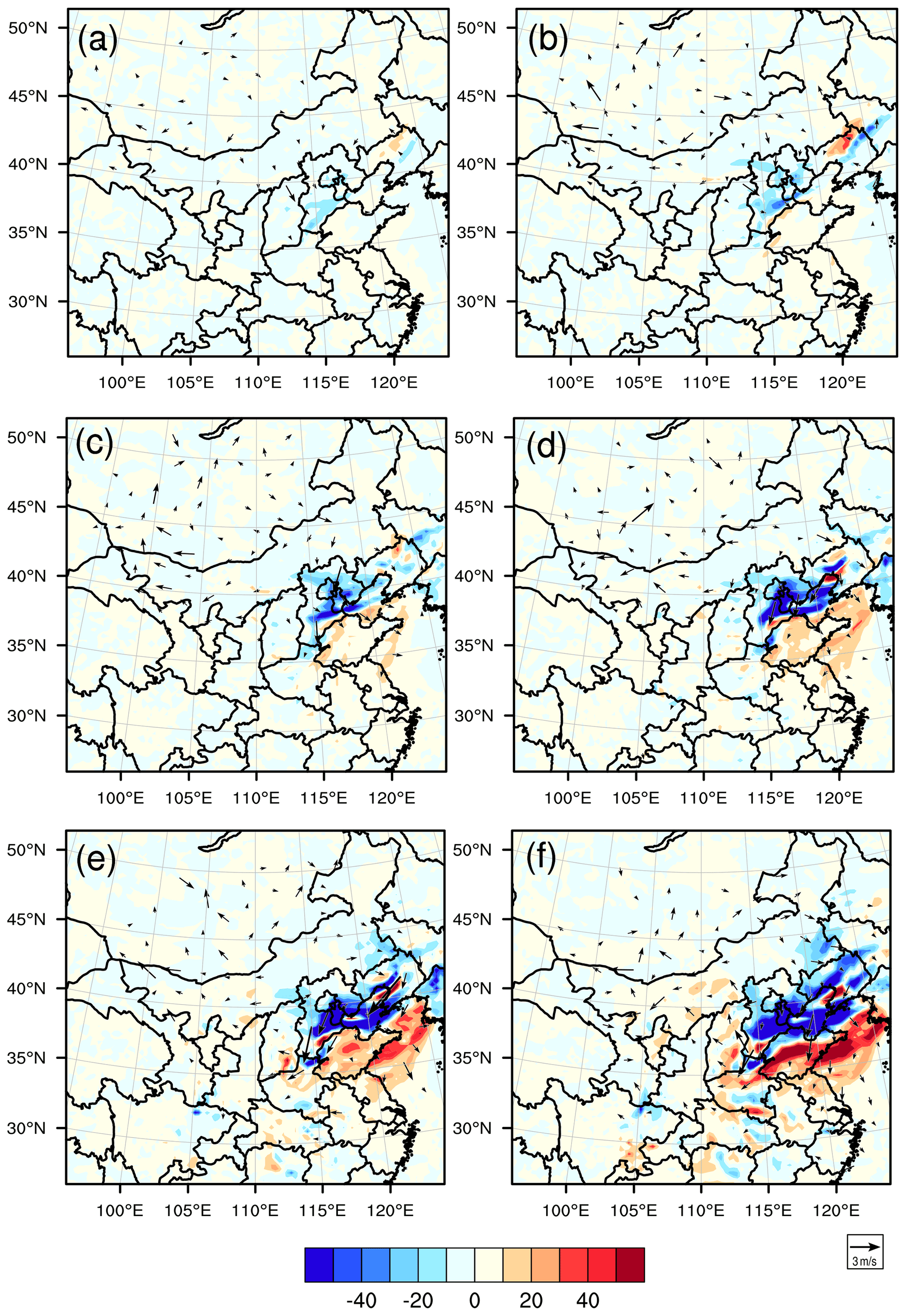
Figure 13The same as Fig. 12 but for the forecast starting from 14:00 BJT on 2 December.
Motivated by the important role of the meteorological initial field in air quality forecasts, we make the first attempt at applying a targeted meteorological field observation strategy with a CNOP approach to improve PM2.5 forecasts using the WRF-NAQPMS model. By considering a heavy haze episode that occurred from 30 November to 4 December 2017 in the Beijing–Tianjin–Hebei region, we explore the effect of possible targeted observations on PM2.5 forecasts during both the accumulation and dissipation periods of the haze event, where the targeted observations are represented by observation arrays consisting of 15 evenly and horizontally distributed grids through four pressure levels (i.e. 950, 850, 750 and 500 hPa) in the sensitive areas identified by the CNOP-type errors, including horizontal wind, temperature and relative humidity components.
To improve the PM2.5 forecast during the accumulation and dissipation periods of the haze event, forecasts with lead times of both 12 and 24 h are investigated, where the AT (i.e. accumulation time, 02:00 BJT on 2 December) and DT (i.e. dissipation time, 14:00 BJT on 3 December) are selected as the verification times (i.e. the forecast times). We first calculate the CNOP-type errors for these four forecasts separately. Then, since the CNOP-type errors concentrate on different vertical levels and in different horizontal areas for different meteorological variables, including wind, temperature and moisture components, we propose using the vertical integral of CNOP-type errors to measure the comprehensive sensitivity of initial errors and to determine the sensitive areas for targeted observations of meteorological fields associated with the PM2.5 forecasts. For the verification time AT, the results show that the sensitive areas identified by CNOP-type errors mainly concentrate in Dezhou and central Inner Mongolia for a lead time of 24 h and in Beijing and Tianjin for a lead time of 12 h. For the verification time DT, the sensitive areas are determined as the region from Hohhot in Inner Mongolia to the Altai Mountains in Mongolia for a lead time of 24 h and the region around Zhangjiakou and Chengde for a lead time of 12 h.
Numerically, we conducted a series of OSSEs to explore whether the possible targeted observations in the above sensitive areas can improve the PM2.5 forecasts of the BTH region and to infer the usefulness of these sensitive areas in implementing practical field observations. For each of the four forecasts, we tried different observation arrays of 15 evenly and horizontally distributed grids through four pressure levels in the sensitive areas and assimilated them to the initial fields for evaluating the improvement of PM2.5 forecasting skill, finally suggesting a more useful observation array for improving the forecasts at the AT and DT. Specifically, for the forecast at the AT, the observation array with a grid space of 90 km in the sensitive area is more effective for a 24 h lead time, and a grid space of 150 km performs the best for a 12 h lead time; however, for the forecast at the DT, the observation array of a grid space of 150 km leads to a better forecasting skill at a 24 h lead time, while that with a grid space of 90 km results in a higher forecasting skill at a 12 h lead time. To further confirm the usefulness of CNOP in identifying the sensitive areas for targeted observations, we compare the improvements of PM2.5 forecasts after assimilating targeted observations in the sensitive areas and the additional observations in the areas along the southwestern (Region-W) and northern (Region-N) directions of the BTH region suggested by previous studies. The results show that the improvements in the PM2.5 forecasting skill when using the additional observations deployed in Region-W and Region-N are significantly smaller than those in the sensitive areas determined by the CNOP approach. More specifically, assimilating the additional observations over Region-W and Region-N cannot ensure a positive forecast benefit. All of these results indicate that preferentially implementing additional observations in the sensitive area determined by the CNOP approach is more likely to significantly improve the PM2.5 forecasts.
Physically, we interpret the reason why the possible targeted observations can significantly improve the PM2.5 forecasting skill by comparing the relevant meteorological fields before and after assimilation. Since the interpretation and its related mechanisms are similar for the forecasts with lead times of 12 and 24 h, we present only the interpretations in detail for the forecast with a lead time of 24 h. During the accumulation process, the control run forecasts a weaker southerly wind and a less stable boundary layer at the AT, which is unfavourable for the accumulation of PM2.5 and finally leads to a severe underestimation of PM2.5 at the AT. When the targeted observations are assimilated to the control run, the southerly wind increases in the southern part of the BTH region at the initial state and finally enhances the southerly wind over the BTH region at the verification time. The increased southerly wind transports more PM2.5 from the south to the BTH region and improves the PM2.5 forecasting skills of the control run at the AT. The assimilation also induces a more stable boundary layer in the assimilation run, which contributed to the increased ground level PM2.5 pollution and improved the PM2.5 forecast skill. For the forecast at the DT, the control run exhibits large southerly wind and positive temperature and relative humidity biases, which prevents the dissipation of PM2.5 and results in an overestimation of PM2.5 at the DT. When the targeted observations are assimilated to the control run, the northerly wind increases and the temperature and relative humidity decrease in the sensitive areas at the initial state. The increased northerly wind drives the cool air in the sensitive area southward and finally blows more PM2.5 from the BTH region to the south, which improves the PM2.5 forecasting skills of the control run at the DT.
The present study provides numerical and physical evidence that the sensitive areas of meteorological initial fields associated with the PM2.5 forecasts indeed exist and that deploying targeted observations of meteorological fields in the sensitive areas determined by the CNOP approach can significantly improve PM2.5 forecasts. Such results formulate a theoretical basis to implement practical field campaigns associated with air quality forecasts. In the practical field campaigns, although the reanalysis data cannot be obtained in time, one can choose the forecast data from ECMWF, which are currently widely regarded as the best and most reliable forecast data, as the initial field to yield a better forecast. Based on this forecast, one can compute the CNOP-type error to identify the sensitive area and design the relevant field observation networks. Such ideas have been applied on real-time typhoon forecasting and have been verified to be able to greatly improve typhoon forecasting skills (Duan and Qin, 2022; Qin et al., 2022). It is also noted that even if sufficient observations exist, the results in the present study can tell us which area of the observations should be preferentially assimilated to improve air quality forecasts.
As this is the first attempt to study the effect of targeted meteorological observations on air quality forecasts, we only utilized one event, and in the future more events should be investigated to obtain a systematic and comprehensive conclusion about how to deploy targeted observations to improve PM2.5 forecasts. Meanwhile, in the present study, finite meteorological variables (wind, temperature, pressure and water vapour) are selected to represent the sensitivity of meteorological initial fields in PM2.5 forecasts. Though they are recognized as important meteorological variables in PM2.5 forecasts over the BTH region (Chen et al., 2020), in order to get a comprehensive conclusion, the sensitivities of more meteorological parameters need to be investigated, including boundary layer height and atmospheric stability, which may not belong to an initial value problem but can be explored by the extension of CNOP method, such as via CNOP-parametric perturbation (CNOP-P; Mu et al., 2010) or a non-linear forcing singular vector method (Duan and Zhou, 2013). In addition, a WRF with the horizontal resolution of 30 km was preliminarily tried in the present study. It is beyond doubt that this resolution is relatively low for the PM2.5 forecasts. Nevertheless, the sensitive areas revealed in the present study are still instructive for practical field observations of PM2.5 forecasts because of the verifications through a series of OSSEs and the reasonable physical interpretation shown in this context. In any case, a WRF with much higher resolution should be used in the future. In addition, only two verification times were adopted for determining sensitive areas, and the dependence of sensitive areas on forecasting times was not explored; both of these issues will be addressed in future work.
In addition to meteorological inputs, emissions are also a key input for air quality forecasts. Accurate emission inputs are difficult enough in terms of their high uncertainties in time and 3-D space, and it is also challenging to satisfy the need for highly confident simulations of a specific event (Peng et al., 2017). Targeted observations may be a better strategy to improve the quality of emissions, and the determination of sensitive areas of emissions is certainly important. Previous studies have adopted the singular vector decomposition and adjoint sensitivity methods to identify the sensitive area for the emissions (Daescu and Carmichael, 2003; Goris and Elbern, 2013). However, it should be noted that these two strategies are based on linear approximation of initial error evolutions, and deploying the observations over the sensitive areas identified by these two strategies may not result in the largest improvement over the verification area, especially for the medium- and long-range forecasts (Wang et al., 2011). Our current study represents the first step in studies of targeted observation of meteorological variable strategies associated with air quality forecasts via the application of CNOP, and only observations of meteorological fields are explored. Thus, targeted observations of emissions based on the CNOP approach are expected to be studied for air quality forecasts in the future.
Hourly surface PM2.5 data are obtained from China National Environmental Monitoring Center (CNEMC, http://www.cnemc.cn/en/, CNEMC, 2022). The ERA5 reanalysis product is available at https://www.ecmwf.int/en/forecasts/datasets/reanalysis-datasets/era5 (Hersbach et al., 2017). The NCEP GFS product is available at https://rda.ucar.edu/datasets/ds084.1/ (NCEP, 2015). The data generated and/or analyzed during this study are stored on the computers at the State Key Laboratory of Numerical Modeling for Atmospheric Sciences and Geophysical Fluid Dynamics and will be available to researchers upon request.
YL, DW and WZ conceived the research. YL and DW designed the experiments, performed the simulations and analysed the results. All authors contributed to the final drafting of the paper.
The contact author has declared that none of the authors has any competing interests.
Publisher's note: Copernicus Publications remains neutral with regard to jurisdictional claims in published maps and institutional affiliations.
The authors highly appreciate the two anonymous reviewers, who provided constructive comments that greatly improved the overall quality of the paper. The study was supported by the National Natural Science Foundation of China (grant nos. 42105061, 42142039 and 41930971).
This research has been supported by the National Natural Science Foundation of China (grant nos. 42105061, 42142039 and 41930971).
This paper was edited by Rob MacKenzie and reviewed by two anonymous referees.
Beal, L. M., Vialard, J., Roxy, M. K., Li, J., Andres, M., Annamalai, H., Feng, M., Han, W., Hood, R., Lee, T., Lengaigne, M., Lumpkin, R., Masumoto, Y., McPhaden, M. J., Ravichandran, M., Shinoda, T., Sloyan, B. M., Strutton, P. G., Subramanian, A. C., Tozuka, T., Ummenhofer, C. C., Unnikrishnan, A. S., Wiggert, J., Yu, L., Cheng, L., Desbruyères, D. G., and Parvathi, V.: A Road Map to IndOOS-2: Better Observations of the Rapidly Warming Indian Ocean, B. Am. Meteorol. Soc., 101, E1891–E1913, https://doi.org/10.1175/BAMS-D-19-0209.1, 2020.
Birgin, E. G., Martinez, J. M., and Raydan, M.: Algorithm 813: SPG – software for convex-constrained optimization, ACM. Trans. Math. Softw., 27, 340–349, https://doi.org/10.1145/502800.502803, 2001.
Bei, N., Wu, J., Elser, M., Feng, T., Cao, J., El-Haddad, I., Li, X., Huang, R., Li, Z., Long, X., Xing, L., Zhao, S., Tie, X., Prévôt, A. S. H., and Li, G.: Impacts of meteorological uncertainties on the haze formation in Beijing–Tianjin–Hebei (BTH) during wintertime: a case study, Atmos. Chem. Phys., 17, 14579–14591, https://doi.org/10.5194/acp-17-14579-2017, 2017.
Chen, Z., Chen, D., Zhao, C., Kwan, M., Cai, J., Zhuang, Y., Zhao, B., Wang, X., Chen, B., Yang, J., Li, R., He, B., Gao, B., Wang, K., and Xu, B.: Influence of meteorological conditions on PM2.5 concentrations across China: A review of methodology and mechanism, Environ. Int., 139, 105558, https://doi.org/10.1016/j.envint.2020.105558, 2020.
China National Environmental Monitoring Centre (CNEMC): Air quality data in China, CNEMC [data set], http://www.cnemc.cn/en/, last access: 30 August 2022.
Da, L. L., Guo, W. H., Cui, B. L., and Liu, J. Y.: Ocean acoustic sensitive region diagnose and adaptive observation, J. Appl. Acoust., 38, 553–561, https://doi.org/10.11684/j.issn.1000-310X.2019.04.012, 2019.
Daescu, D. N. and Carmichael, G. R.: An Adjoint Sensitivity Method for the Adaptive Location of the Observations in Air Quality Modeling, J. Atmos. Sci., 60, 434–450, https://doi.org/10.1175/1520-0469(2003)060<0434:AASMFT>2.0.CO;2, 2003.
Duan, W. S. and Qin, X. H.: Application of nonlinear optimal perturbation methods in the targeting observations and field campaigns of tropical cyclones, Advances in Earth Science, 37, 165–176, https://doi.org/10.11867/j.issn.1001-8166.2022.010, 2022 (in Chinese).
Duan, W. S. and Zhou, F. F.: Non-linear forcing singular vector of a two-dimensional quasi-geostrophic model, Tellus, 65, 256, https://doi.org/10.3402/tellusa.v65i0.18452, 2013.
Duan, W. S., Li, X. Q., and Tian, B.: Towards optimal observational array for dealing with challenges of El Niño-Southern Oscillation predictions due to diversities of El Niño, Clim. Dynam., 51, 3351–3368, https://doi.org/10.1007/s00382-018-4082-x, 2018.
Dudhia, J.: Numerical study of convection observation during the winter monsoon experiment using a mesoscale two-dimensional model, J. Atmos., Sci., 46, 3077–3107, https://doi.org/10.1175/1520-0469(1989)046<3077:NSOCOD>2.0.CO;2, 1989.
Ehrendorfer, M., Errico, R. M., and Raeder, K. D.: Singular-Vector Perturbation Growth in a Primitive Equation Model with Moist Physics, J. Atmos. Sci., 56, 1627–1648, https://doi.org/10.1175/1520-0469(1999)056<1627:SVPGIA>2.0.CO;2, 1999.
Feng, R., Duan, W., and Mu, M.: Estimating observing locations for advancing beyond the winter predictability barrier of Indian Ocean Dipole event predictions, Clim. Dynam., 48, 1173–1185, https://doi.org/10.1007/s00382-016-3134-3, 2017.
Feng, T., Li, G., Cao, J., Bei, N., Shen, Z., Zhou, W., Liu, S., Zhang, T., Wang, Y., Huang, R.-J., Tie, X., and Molina, L. T.: Simulations of organic aerosol concentrations during springtime in the Guanzhong Basin, China, Atmos. Chem. Phys., 16, 10045–10061, https://doi.org/10.5194/acp-16-10045-2016, 2016.
Gilliam, R. C., C. Hogrefe, J. M., Godowitch, S., Napelenok, R. M., and Rao, S. T.: Impact of inherent meteorology uncertainty on air quality model predictions, J. Geophys. Res.-Atmos., 120, 12259–12280, https://doi.org/10.1002/2015JD023674, 2015.
Godowitch, J. M., Gilliam, R. C., and Rao, S. T.: Diagnostic evaluation of the chemical and transport processes in a regional photochemical air quality modeling system, Atmos. Environ., 45, 3977–3987, https://doi.org/10.1016/j.atmosenv.2011.04.062, 2011.
Goris, N. and Elbern, H.: Singular vector decomposition for sensitivity analyses of tropospheric chemical scenarios, Atmos. Chem. Phys., 13, 5063–5087, https://doi.org/10.5194/acp-13-5063-2013, 2013.
Guan, W. J., Zheng, X. Y., Chung, K. F., and Zhong, N. S.: Impact of air pollution on the burden of chronic respiratory diseases in China: time for urgent action, Lancet 388, 1939–1951, https://doi.org/10.1016/S0140-6736(16)31597-5, 2016.
He, J., Gong, S., Yu, Y., Yu, L., Wu, L., Mao, H., Song, C., Zhao, S., Liu, H., Liu, X., and Li, R.: Air pollution characteristics and their relation to meteorological conditions during 2014–2015 in major Chinese cities, Environ. Pollut., 223, 484–496, https://doi.org/10.1016/j.envpol.2017.01.050, 2017.
Hersbach, H., Bell, B., Berrisford, P., Hirahara, S., Horányi, A., Muñoz‐Sabater, J., Nicolas, J., Peubey, C., Radu, R., Schepers, D., Simmons, A., Soci, C., Abdalla, S., Abellan, X., Balsamo, G., Bechtold, P., Biavati, G., Bidlot, J., Bonavita, M., De Chiara, G., Dahlgren, P., Dee, D., Diamantakis, M., Dragani, R., Flemming, J., Forbes, R., Fuentes, M., Geer, A., Haimberger, L., Healy, S., Hogan, R. J., Hólm, E., Janisková, M., Keeley, S., Laloyaux, P., Lopez, P., Lupu, C., Radnoti, G., de Rosnay, P., Rozum, I., Vamborg, F., Villaume, S., and Thépaut, J.-N.: Complete ERA5 from 1979: Fifth generation of ECMWF atmospheric reanalyses of the global climate. Copernicus Climate Change Service (C3S) Data Store (CDS), ECMWF [data set], https://www.ecmwf.int/en/forecasts/datasets/reanalysis-datasets/era5, (last access: 30 August 2022), 2017.
Hong, S. Y., Ying, N., and Dudhia, J.: A new vertical diffusion package with an explicit treatment of entrainment processes, Mon. Weather Rev., 134, 2318–2341, https://doi.org/10.1175/MWR3199.1, 2006.
Hu, J. L., Ying, Q., and Chen, J. J.: Particulate air quality model predictions using prognostic vs. diagnostic meteorology in central California, Atmos. Environ., 44, 215–226, https://doi.org/10.1016/j.atmosenv.2009.10.011, 2010.
Iacono, M. J., Delamere, J. S., Mlawer, E. J., Shephard, M. W., Clough, S. A., Collins, W. D.: Radiative forcing by long-lived greenhouse gases: calculations with the AER radiative transfer models, J. Geophys. Res.-Atmos., 113, D13103, https://doi.org/10.1029/2008JD009944, 2008.
Janjić, T., Bormann, N., Bocquet, M., Carton, J. A., Cohn, S. E., Dance, S. L., Losa, S. N., Nichols, N. K., Potthast, R., Waller, J. A., and Weston, P.: On the representation error in data assimilation, Q. J. Roy. Meteor. Soc., 144, 1257–1278, https://doi.org/10.1002/qj.3130, 2018.
Kong, Y. W., Sheng, L. F., Li, Y. P., Zhang, W. H., Zhou, Y., Wang, W. C., and Zhao, Y. H.: Improving PM2.5 forecast during haze episodes over China based on a coupled 4D-LETKF and WRF-Chem system, Atmos. Res., 249, 105366, https://doi.org/10.1016/j.atmosres.2020.105366, 2021.
Kramer, W. and Dijkstra, H. A.: Optimal localized observations for advancing beyond the ENSO predictability barrier, Nonlin. Processes Geophys., 20, 221–230, https://doi.org/10.5194/npg-20-221-2013, 2013.
Kren, A. C., Cucurull, L., and Wang, H.: Addressing the sensitivity of forecast impact to flight path design for targeted observations of extratropical winter storms: A demonstration in an OSSE framework, Meteorol. Appl., 27, e1942, https://doi.org/10.1002/met.1942, 2020.
Kumar, R., Delle Monache, L., Bresch, J., Saide, P. E., Tang, Y., Liu, Z., da Silva, A., Alessandrini, S., Pfister, G., Edwards, D., Lee, P., and Djalalova, I.: Toward improving Short-Term predictions of Fine Particulate Matter over the United States Via Assimilation of Satellite Aerosol Optical Depth Retrievals, J. Geophys. Res.-Atmos., 124, 2753–2773, https://doi.org/10.1029/2018JD029009, 2019.
Li, M., Zhang, Q., Streets, D. G., He, K. B., Cheng, Y. F., Emmons, L. K., Huo, H., Kang, S. C., Lu, Z., Shao, M., Su, H., Yu, X., and Zhang, Y.: Mapping Asian anthropogenic emissions of non-methane volatile organic compounds to multiple chemical mechanisms, Atmos. Chem. Phys., 14, 5617–5638, https://doi.org/10.5194/acp-14-5617-2014, 2014.
Li, Y. Q., Yu, L., and Chen B. D.: An Assessment of Design of Observation Network over the Tibetan Plateau Based on Observing System Simulation Experiments (OSSE), J. Meteorol. Soc. Jpn., 93, 343–358, https://doi.org/10.2151/jmsj.2015-019, 2015.
Lim, C. and Thurston, G.: Air Pollution, Oxidative Stress, and Diabetes: A Life Course Epidemiologic Perspective, Current Diabetes Rep., 19, 58, https://doi.org/10.1007/s11892-019-1181-y, 2019.
Lin, Y. L., Farley, R. D., and Orville, H. D.: Bulk Parameterization of the Snow Field in a Cloud Model, Clim. Appl. Meteorol., 22, 1065–1092, https://doi.org/10.1175/1520-0450(1983)022<1065:BPOTSF>2.0.CO;2, 1983.
Liu, N., Duan, W. S., Wang, Z. F., Tang, X., and Zhou, F. F.: A Study on Target Observation of a Heavy Air Pollution Event in Beijing, Clim. Environ. Res., 23, 619–632, https://doi.org/10.3878/j.issn.1006-9585.2018.18025, 2018.
Liu, Z. X., Liu, S. H., Hu, F., Li J., Ma, Y. J., and Liu, H. P.: A comparison study of the simulation accuracy between WRF and MM5 in simulating local atmospheric circulations over Greater Beijing, Science China, 55, 418–427, https://doi.org/10.1007/s11430-011-4310-2, 2012.
Lorenz, E. N.: A study of the predictability of a 28-variable atmospheric model, Tellus, 17, 321–333, https://doi.org/10.1111/j.2153-3490.1965.tb01424.x, 1965.
Majumdar, S.: A Review of Targeted Observations, B. Am. Meteorol. Soc., 97, 2287–2303, https://doi.org/10.1175/BAMS-D-14-00259.1, 2016.
Masutani, M., Schlatter, T., Errico, R., Stoffelen, A., Andersson, E., Lahoz, W., Woollen, J., Emmitt, G., Riishojgaard, L., and Lord, S.: Observing System Simulation Experiments, in: Data Assimilation, edited by: Lahoz, W., Khattatov, B., and Menard, R., Springer, Berlin, Heidelberg, https://doi.org/10.1007/978-3-540-74703-1_24, 2010.
Miao, Y. C., Hu, X. M., Liu, S. H., Qian, T. T., Xue, M., Zheng, Y. J., and Wang, S.: Seasonal variation of local atmospheric circulations and boundary layer structure in the Beijing-Tianjin-Hebei region and implications for air quality, J. Adv. Model. Earth Sy., 7, 1602–1626, 2015.
Mu, M. and Zhang, Z. Y.: Conditional nonlinear optimal perturbations of a two-dimensional Quasigeostrophic model, J. Atmos. Sci., 63, 1587–1604, https://doi.org/10.1175/JAS3703.1, 2006.
Mu, M., Duan, W. S., and Wang, B.: Conditional nonlinear optimal perturbation and its applications, Nonlin. Processes Geophys., 10, 493–501, https://doi.org/10.5194/npg-10-493-2003, 2003.
Mu, M., Zhou, F. F., and Wang, H. L.: A method to identify the sensitive areas in targeting for tropical cyclone prediction: Conditional Nonlinear optimal perturbation, Mon. Weather Rev., 137, 1623–1639, https://doi.org/10.1175/2008MWR2640.1, 2009.
Mu, M., Duan, W., Wang, Q., and Zhang, R.: An extension of conditional nonlinear optimal perturbation approach and its applications, Nonlin. Processes Geophys., 17, 211–220, https://doi.org/10.5194/npg-17-211-2010, 2010.
Mu, M., Duan, W. S., Chen, D. K., and Yu, W. D.: Target observations for improving initialization of high-impact ocean-atmospheric environmental events forecasting, Natl. Sci. Rev., 2, 226–236, https://doi.org/10.1093/nsr/nwv021, 2015.
NCEP: NCEP GFS 0.25 Degree Global Forecast Grids Historical Archive, NCEP [data set], https://doi.org/10.5065/D65D8PWK, 2015.
Palmer, T. N., Gelaro, R., Barkmeijer, J., and Buizza, R.: Singular vectors, metrics, and adaptive observations, J. Atmos. Sci., 55, 633–653, https://doi.org/10.1175/1520-0469(1998)055<0633:SVMAAO>2.0.CO;2, 1998.
Peng, Z., Liu, Z., Chen, D., and Ban, J.: Improving PM2.5 forecast over China by the joint adjustment of initial conditions and source emissions with an ensemble Kalman filter, Atmos. Chem. Phys., 17, 4837–4855, https://doi.org/10.5194/acp-17-4837-2017, 2017.
Qin X., Duan, W., and Mu, M.: Conditions under which CNOP sensitivity is valid for tropical cyclone adaptive observations, Q. J. Roy. Meteor. Soc., 139, 1544–1554, https://doi.org/10.1002/qj.2109, 2013.
Qin, X., Duan, W. S., Pak, W. C., Chen, B. Y., and Kang-Ning, H.: Effects of dropsonde data in field campaigns on forecasts of tropical cyclones over the western North Pacific in 2020 and role of CNOP sensitivity, Adv. Atmos. Sci., in press, https://doi.org/10.1007/s00376-022-2136-9, 2022.
Romano, D., Bernetti, A., and De Lauretis, R.: Different methodologies to quantify uncertainties of air emissions, Environ. Int., 30, 1099–1107, https://doi.org/10.1016/j.envint.2004.06.006, 2004.
Snyder, C.: Summary of an informal workshop on adaptive observations and FASTEX, B. Am. Meteorol. Soc., 77, 953–961, https://doi.org/10.1175/1520-0477-77.5.953, 1996.
Sun, J., Gong, J. H., Zhou, J. P., Liu, J. T., and Liang, J. M.: Analysis of PM2.5 pollution episodes in Beijing from 2014 to 2017: classification, interannual variations and associations with meteorological features, Atmos. Environ., 213, 384–394, https://doi.org/10.1016/j.atmosenv.2019.06.015, 2019.
Wang, H., Mu, M., and Huang, X.-Y.: Application of conditional non-linear optimal perturbations to tropical cyclone adaptive observation using the Weather Research Forecasting (WRF) model, Tellus A, 63, 939–957, https://doi.org/10.1111/j.1600-0870.2011.00536.x, 2011.
Wang, Z. F., Xie, F. Y., Wang, X. Q., An, J. L., and Zhu, J.: Development and application of nested air quality prediction modeling system, Chin. J. Atmos. Sci., 30, 778e790, https://doi.org/10.3878/j.issn.1006-9895.2006.05.07, 2006.
Wang, Z. F., Huang, M. Y., He, D., Xu, H. Y., and Zhou, L.: Studies on transport of acid substance in China and East Asia part I: 3-D Eulerian transport model for pollutants, Chin. J. Atmos. Sci., 21, 367e375, https://doi.org/10.3878/j.issn.1006-9895.1997.03.14, 1997.
Wu, C. C., Majumdar, S., Peng, M. S., and Aberson, S.: Intercomparison of Targeted Observation Guidance for Tropical Cyclones in the Northwestern Pacific, Mon. Weather Rev., 137, 2471–2492, https://doi.org/10.1175/2009MWR2762.1, 2009.
Xu, T., Song, Y., Liu, M., Cai, X., Zhang, H., Guo, J., and Zhu, T.: Temperature inversions in severe polluted days derived from radiosonde data in North China from 2011 to 2016, Sci. Total Environ., 647, 1011–1020, https://doi.org/10.1016/j.scitotenv.2018.08.088, 2019.
Yang, W., Chen, H., Wu, J., Wang, W., and Wang, W.: Characteristics of the source apportionment of primary and secondary inorganic PM2.5 in the pearl river delta region during 2015 by numerical modeling, Environ. Pollut., 267, 115418, https://doi.org/10.1016/j.envpol.2020.115418, 2020.
Yu, Y., Mu, M., Duan, W., and Gong, T.: Contribution of the location and spatial pattern of initial error to uncertainties in El Niño predictions, J. Geophy. Res., 117, C06018, https://doi.org/10.1029/2011JC007758, 2012.
Zhang, F., Bei, N., Nielsen-Gammon, J. W., Li, G., Zhang, R., Stuart, A. L., and Aksoy, A.: Impacts of meteorological uncertainties on ozone pollution predictability estimated through meteorological and photochemical ensemble forecasts, J. Geophys. Res., 112, D04304, https://doi.org/10.1029/2006JD007429, 2007.
Zhang, H., Yuan, H. O., Liu, X. H., Yu, J. Y., and Jiao, Y. L.: Impact of synoptic weather patterns on 24h-average PM2.5 concentrations in the North China Plain during 2013–2017, Sci. Total Environ., 627, 200–210, https://doi.org/10.1016/j.scitotenv.2018.01.248, 2018.
Zhang, K., Mu, M., Wang, Q., Yin, B., and Liu, S.: CNOP-based adaptive observation network designed for improving upstream kuroshio transport prediction, J. Geophy. Res.-Oceans, 124, 4350–4364, https://doi.org/10.1029/2018JC014490, 2019.
Zhang, X., Fung, J. C. H., Lau, A. K. H., Zhang, S., and Huang, W.: Improved modeling of spatiotemporal variations of fine particulate matter using a three-dimensional variational data fusion method, J. Geophys. Res.-Atmos., 126, e2020JD033599, https://doi.org/10.1029/2020JD033599, 2021.
Zhao, X., Zhang, X., Xu, X., Xu, J., Meng, W., and Pu, W.: Seasonal and diurnal variations of ambient PM2.5, concentration in urban and rural environments in Beijing, Atmos. Environ., 43, 2893–2900, https://doi.org/10.1016/j.atmosenv.2009.03.009, 2009.
- Abstract
- Introduction
- Model, methodology and data
- The CNOP of the PM2.5 forecasting
- The sensitive area for targeted observations and associated validity verification on improving the PM2.5 forecasts
- Interpretation
- Summary and discussion
- Data availability
- Author contributions
- Competing interests
- Disclaimer
- Acknowledgements
- Financial support
- Review statement
- References