Below-cloud scavenging of aerosol by rain: a review of numerical modelling approaches and sensitivity simulations with mineral dust in the Met Office's Unified Model

Theoretical models of the below-cloud scavenging (BCS) of aerosol by rain yield scavenging rates that are 1–2 orders of magnitude smaller than observations and associated empirical schemes for submicron-sized aerosol. Even when augmented with processes which may explain this disparity, such as phoresis and rear capture in the raindrop wake, the theoretical BCS rates remain an order of magnitude less than observations. Despite this disparity, both theoretical and empirical BCS schemes remain in wide use within numerical aerosol models. BCS is an important sink for atmospheric aerosol, in particular for insoluble aerosol such as mineral dust, which is less likely to be scavenged by in-cloud processes than purely soluble aerosol. In this paper, various widely used theoretical and empirical BCS models are detailed and then applied to mineral dust in climate simulations with the Met Office's Unified Model in order the gauge the sensitivity of aerosol removal to the choice of BCS scheme. We show that the simulated accumulation-mode dust lifetime ranges from 5.4 d in using an empirical BCS scheme based on observations to 43.8 d using a theoretical scheme, while the coarse-mode dust lifetime ranges from 0.9 to 4 d, which highlights the high sensitivity of dust concentrations to BCS scheme. We also show that neglecting the processes of rear capture and phoresis may overestimate submicron-sized dust burdens by 83 %, while accounting for modal widths and mode merging in modal aerosol models alongside BCS is important for accurately reproducing observed aerosol size distributions and burdens. This study provides a new parameterisation for the rear capture of aerosol by rain and is the first to explicitly incorporate the rear-capture mechanism in climate model simulations. Additionally, we answer many outstanding questions pertaining to the numerical modelling of BCS of aerosol by rain and provide a computationally inexpensive BCS algorithm that can be readily incorporated into other aerosol models.

1 Introduction

Atmospheric aerosols play an important role in climate system by altering energy fluxes, interacting with clouds, transferring nutrients to ecosystems, and contributing to atmospheric chemistry and air quality (Haywood and Boucher, 2000). For these reasons, it is vital that aerosol microphysical processes are accurately modelled in general circulation models (GCMs), especially given that aerosol–climate interactions are one of the leading causes of uncertainty in existing GCMs (Carslaw et al., 2013). Aerosols are efficiently removed from the troposphere by wet deposition processes such as in-cloud scavenging (ICS) (also denoted “rainout” or “nucleation scavenging”) and below-cloud scavenging (BCS) (also denoted “washout” or “impaction scavenging”) (Pruppacher and Klett, 2010). ICS occurs when aerosols act as cloud condensation nuclei and form cloud droplets or ice crystals which then grow and fall as precipitation or when aerosols collide with existing cloud droplets. BCS occurs when falling hydrometeors, such as rain or snow, irreversibly collect ambient aerosol in their path. The BCS rate strongly depends on the rain intensity, raindrop size distribution, and the collection efficiency between raindrops and aerosol particles (Laakso et al., 2003).

A long-established problem in BCS modelling is reconciling BCS rates from in situ atmospheric observations with rates derived from conceptual models and laboratory experiments (Beard, 1974; Davenport and Peters, 1978; Radke et al., 1980; Volken and Schumann, 1993; Laakso et al., 2003). In particular, BCS rates from theoretical models are 1–2 orders of magnitude smaller than observed rates for accumulation-sized (diameters of $\mathrm{0.1}\le d_{\mathrm{p}}\le \mathrm{1}$ µm) particles (Wang et al., 2010). Given that accumulation aerosols are particularly important to the climate system for cloud microphysics, radiative interactions, heterogeneous chemistry, air quality, and myriad other climate interactions, it is important to represent aerosol microphysics accurately in GCMs. The accumulation size range, where BCS rates exhibit a global minimum owing to the lack of a dominant scavenging process, is widely denoted the “Greenfield gap”, and the scavenging minimum is seen in both observations and theory, albeit with different magnitudes (Greenfield, 1957).

Various hypotheses have been put forward to explain the disparity between observations and theory. Beard (1974) and Davenport and Peters (1978) suggested that aerosol hygroscopic growth and electrostatic charge effects, which are not explicitly modelled by the early theoretical models, may explain the disparity. Quérel et al. (2014) highlighted the effect of downdrafts caused by the falling precipitation on near-surface aerosol concentrations, with comparatively clean air transported downward from aloft possibly masking the direct BCS effect. Additional uncertainty arises from modelling BCS by millimetre-sized raindrops given their tendency to oscillate in free fall, with complex flows leading to enhanced rear-capture and frontal-capture effects (Wang and Pruppacher, 1977; Lemaitre et al., 2017). Although atmospheric turbulence has been imputed for the disparity between observations and theory (e.g. Wang et al., 2010, 2011), Vohl et al. (2001) found little impact of turbulence on BCS rates in their laboratory experiments with larger raindrops (diameters D_d≥600 µm). A recent hypothesis is that the enhanced BCS rates from observations may be due to contributions from ICS and other confounding atmospheric processes such as turbulent diffusion, given that it is difficult to conduct a controlled BCS experiment in the actual atmosphere (Andronache et al., 2006; Wang et al., 2011). Indeed, BCS rates determined from the controlled “outdoor” experiment of Sparmacher et al. (1993), in which monodisperse aerosol in a wind-shielding chamber was subjected to natural precipitation, were much closer to theoretical values than other observational values (Wang et al., 2010).

The disparity between observed and theoretical BCS rates has stimulated a wide range of approaches of varying complexity for modelling BCS in GCMs (Jung et al., 2003; Croft et al., 2009, 2010; Wang et al., 2010, 2014). The most widely utilised theoretical BCS approach in GCMs is to follow Slinn (1984) in expressing the raindrop–particle collection efficiency – an important BCS parameter representing the ratio of number of collisions between a raindrop and particles to the total number of particles in an area equal to the raindrop's cross-sectional area – as a linear combination of collection efficiencies due to Brownian motion, inertial impaction, and interception (Seinfeld and Pandis, 1998; Jung et al., 2003; Loosmore et al., 2004; Berthet et al., 2010; Wang et al., 2010). Slinn (1984) proposed formulae for the individual collection efficiencies based on data from laboratory experiments and dimensional analyses. Other processes are known to contribute to BCS including thermophoresis and diffusiophoresis, by which particles move along temperature and water gradients respectively, and attraction between oppositely charged raindrops and particles (Slinn and Hales, 1971; Davenport and Peters, 1978; Andronache, 2004; Andronache et al., 2006). Recently, Lemaitre et al. (2017) compared results from historical numerical models, with and without the assumption of Stokes flow, to derive an empirical formula for the collection efficiency in the recirculating flow of the raindrop's wake. Lemaitre et al. (2017) and Quérel et al. (2014) have proposed that this “rear-capture” effect, neglected by Slinn (1984), be directly added to the established processes in BCS schemes. Wang et al. (2010) recommended that the theoretical schemes which yield the highest BCS rates be used in GCMs, while Wang et al. (2014) develop on this suggestion by deriving a semi-empirical formula for the 90 % percentile of theoretical BCS rates from the literature.

An alternative approach to the theoretical modelling of Slinn (1984) and others (e.g. Hall, 1980; Flossmann, 1986) for deriving BCS rates is to empirically fit formulae to observations. Laakso et al. (2003) measured BCS rates over 6 years at a boreal forest site in Southern Finland and then combined these measurements with similar observations from Volken and Schumann (1993), to derive a widely utilised empirical fit for the BCS rate as a function of aerosol size and rain intensity. A similar approach was conducted by Baklanov and Sørensen (2001), who omitted a size dependence in the formulation of BCS rates for Aitken-sized (diameters of $\mathrm{0.01}\le d_{\mathrm{p}}\le \mathrm{0.1}$ µm) and accumulation-sized aerosols. Therein lies the issue with empirical schemes – notably, what to do outside the boundaries of observations. Additionally, rain types differ with location (e.g. in terms of the electric charge density of raindrops), and aerosols differ in composition, and so the general applicability of empirical schemes' fit to data in a single location is questionable (Wang et al., 2014). Note though that similar uncertainties are also present in the theoretical models, which are fit to laboratory data and observations (e.g. the raindrop number distribution is often parameterised as a function of rainfall rate, which is often fit to observations). Size-resolved BCS rates from field data have become increasingly available in recent decades (e.g. Maria and Russell, 2005; Zikova and Zdimal, 2016; Blanco-Alegre et al., 2018, 2021; Cugerone et al., 2018; Lu et al., 2019; Xu et al., 2019) and are generally commensurate between campaigns across the aerosol size spectrum.

The panoply of BCS models used by the aerosol modelling community raises the question of what the implications are of selecting certain BCS models over others. Indeed, it would be useful for the aerosol modelling community to have the following key questions (KQs) answered before designing or selecting a BCS scheme:

• KQ1. To what extent does the use of an empirical BCS model over a theoretical model change atmospheric aerosol concentrations in a GCM?

• KQ2. How important is it to include missing processes in the Slinn (1984) BCS model, notably phoresis and the rear-capture effect? The rear-capture model of Lemaitre et al. (2017) is only valid for a narrow range of aerosol diameters, and thus an improved model – valid for the entire aerosol size spectrum – will be provided and utilised in this study.

• KQ3. Pertaining to modal aerosol schemes, to what extent does the use of a single-moment BCS approach – where BCS rates are computed solely using the aerosol modal median diameter while the width of the mode is ignored – over a double-moment approach change simulated aerosol concentrations?

• KQ4. Pertaining to double-moment modal aerosol schemes, how important is it to include downward mode merging – or the redistribution of aerosol mass and number from a large to a neighbouring smaller mode – alongside BCS?

KQ4 requires further explanation. Many GCMs participating in the AeroCom phase III model intercomparison project employ a double-moment modal aerosol scheme (Gliß et al., 2021). Modal schemes have the advantage over bulk schemes that the aerosol size distribution is permitted to evolve, albeit often within a predefined size bracket and – in the case of double-moment schemes – assuming a fixed modal width. Atmospheric processes such as coagulation, condensation, BCS, ICS, and sedimentation may cause neighbouring modes to evolve such that they overlap and become indistinguishable (Whitby et al., 2002). Additionally, size-dependent processes such as BCS may alter the width of the ambient size mode, and thus a double-moment modal aerosol scheme with fixed geometric widths would be unable to capture this effect. To account for this deficiency in the double-moment architecture, “mode-merging” schemes are often employed to redistribute aerosol mass and number between neighbouring modes (Mann et al., 2010). Given the highly size-dependent nature of BCS, it is useful to test the impact of representing downward mode merging (i.e. the transfer of mass and number from the coarse mode to the smaller accumulation mode when the modes overlap) to account for contraction of the coarse mode as a result of BCS.

To answer the KQs, 20-year integrations are performed with the Met Office's Unified Model (UM) in a climate configuration, where the sole variable is the formulation of BCS applied to mineral dust aerosol. The UM represents aerosol using the double-moment Global Model of Aerosol Processes (GLOMAP-mode) model, which is coupled to the United Kingdom Chemistry and Aerosol (UKCA) model in the UM and cumulatively denoted UKCA-mode (Mann et al., 2010; Mulcahy et al., 2018; Jones et al., 2021). Whilst UKCA-mode has in-built functionality to represent mineral dust in two insoluble modes representing accumulation-sized and coarse-sized (diameters of d_p≥1 µm) particles, this scheme has never been the default option in the Met Office Global Atmosphere science configuration – which forms the physical atmosphere in the UK's Earth system model – owing to the lack of fidelity between simulations and observations, with UKCA-mode dust exhibiting dust concentrations that are too high away from source regions. Inefficient wet removal is thought to be an important factor, which may in part be addressed by the results of this study. Instead, the six-bin dust scheme within the single-moment Coupled Large-scale Aerosol Simulator for Studies in Climate (CLASSIC) aerosol framework (Woodward, 2001) remains the default option in Global Atmosphere version 7.1 (GA7.1) and later versions (Mulcahy et al., 2020). UKCA-mode dust thus appears an ideal candidate for comparing BCS schemes, given its significant potential for improvement. However, the focus of this paper is to look at the underlying BCS theory using the UM, rather than to provide a direct comparison with existing functionality in this model.

The aim of this study is to outline the most widely utilised numerical BCS models and then to compare them quantitatively in UM simulations. In Sect. 2, various BCS models are presented, and a computationally inexpensive BCS algorithm is proposed that can be readily incorporated into other GCMs. In Sect. 3, the box model simulations are described, while in Sect. 4 the UM configuration is described, and the UM simulations are outlined. In Sect. 5, the various numerical BCS approaches are compared using the results of offline box model and UM simulations, in terms of spatio-temporal dust concentrations and deposition rates. In Sect. 6, the results and implications of this study are discussed.

2 Below-cloud scavenging approaches

2.1 Overview of a new BCS algorithm

Fully resolved BCS schemes are computationally expensive to run in GCMs, owing to the need to integrate BCS rates over the aerosol and raindrop size distributions at every time step and in every grid cell that is subject to precipitation. Methods to explicitly compute BCS online include the use of Gauss quadrature (e.g. Berthet et al., 2010) or by simplifying the BCS equation to a polynomial in the aerosol diameter (d_p) and then using the moment method to obtain an analytical solution (e.g. Jung et al., 2003). Alternatively, to reduce the computational cost, the BCS rate can be calculated offline as a function of aerosol and raindrop size properties and standard atmospheric conditions and then tabulated for simple interpolation in a GCM, which is the approach adopted here.

A new BCS algorithm, which has the quality that it is easy to change the underlying BCS parameterisation, is presented in this section. The time-dependent removal of aerosol by BCS is generally expressed as a first-order decay equation (Seinfeld and Pandis, 1998; Wang et al., 2010).

$$\begin{array}{}\text{(1)}& {\displaystyle \frac{\mathrm{d}n\left(d_{\mathrm{p}}\right)}{\mathrm{d}t}}=-\mathrm{\Lambda }\left(d_{\mathrm{p}},R\right)n\left(d_{\mathrm{p}}\right)\text{(2)}& {\displaystyle }\mathrm{\Lambda }\left(d_{\mathrm{p}},R\right)=\underset{\mathrm{0}}{\overset{\mathrm{\infty }}{\int }}{\displaystyle \frac{\mathit{\pi }}{\mathrm{4}}}{D}_{\mathrm{d}}^{\mathrm{2}}{U}_t\left(D_{\mathrm{d}}\right)E\left(d_{\mathrm{p}},D_{\mathrm{d}}\right)N\left(D_{\mathrm{d}};R\right)\mathrm{d}{D}_{\mathrm{d}}\end{array}$$

In Eq. (1), n(d_p) is the size-resolved particle number concentration at time t, d_p is the particle diameter, R is the rainfall rate, and Λ(d_p,R) is the size-resolved BCS rate. Equation (2) expresses Λ(d_p,R) as the integral of the collection kernel $K\left(d_{\mathrm{p}},D_{\mathrm{d}}\right)=\frac{\mathit{\pi }}{\mathrm{4}}{D}_{\mathrm{d}}^{\mathrm{2}}{U}_t\left(D_{\mathrm{d}}\right)E\left(d_{\mathrm{p}},D_{\mathrm{d}}\right)$ over the raindrop size distribution N(D_d;R), where E(d_p,D_d) denotes the particle collection efficiency, U_t(D_d) denotes the raindrop's fall speed, and the raindrop size distribution is often modelled as an empirical function of the rainfall rate R (e.g. Abel and Boutle, 2012). The algorithm assumes two reasonable approximations, firstly that the diameter of the raindrop is significantly greater than of the particle (D_d≫d_p) and secondly that the falling velocity of the raindrop is significantly greater than for the particle (U_t(D_d)≫U_t(d_p)). Generally, it is empirically assumed that the collection efficiency equals the collision efficiency or that all collisions between a hydrometeor and a particle result in successful collection (Weber et al., 1969). Note that mineral dust particles are not usually spherical, so d_p represents an effective diameter. For large raindrops, the shape is also not spherical, so D_d also represents an effective diameter.

For the BCS scheme based on Slinn's (1984) model for E(d_p,D_d) (Sect. 2.2–2.4), U_t(D_d) is parameterised following the “gold standard” method of Beard (1976) (see Sect. S1 in the Supplement). In short, U_t(D_d) is determined for three different raindrop regimes, which is necessary given the sensitivity of flow type to the raindrop diameter. For the raindrop number density N(D_d;R), a recent parameterisation based on Abel and Boutle (2012) (Eq. 3), rather than the Sekhon and Srivastava (1971) model used in the default UKCA-mode BCS scheme, is used in this study (see Sect. S2). Using the Abel and Boutle (2012) scheme for the raindrop number density makes BCS consistent with warm rain assumptions in the UM. In Eq. (3), N₀ and λ are the intercept and slope of the raindrop size distribution, and R is in units of millimetres per hour (mm h⁻¹). Alternative models for N(D_d;R) and U_t(D_d) are provided in Sect. 2.2–2.3 of Wang et al. (2010).

$$\begin{array}{}\text{(3a)}& {\displaystyle }N\left(D_{\mathrm{d}};R\right)& {\displaystyle }=N_{\mathrm{0}}\left(R\right)e^{-\mathit{\lambda }\left(R\right)D_{\mathrm{d}}}\text{(3b)}& {\displaystyle }{N}_{\mathrm{0}}\left(R\right)& {\displaystyle }=\mathrm{4.9}\times {\mathrm{10}}^{\mathrm{7}}{R}^{-\mathrm{0.89}}\text{(3c)}& {\displaystyle }\mathit{\lambda }\left(R\right)& {\displaystyle }=\mathrm{6.236}\times {\mathrm{10}}^{\mathrm{3}}{R}^{-\mathrm{0.4}}\end{array}$$

The approach of Croft et al. (2009, 2010) is adopted to determine number and mass mean BCS rates by integrating Λ(d_p,R) over the aerosol number and mass size distributions (Eqs. 4–5).

$$\begin{array}{}\text{(4)}& {\displaystyle }{\mathrm{\Lambda }}_N\left(\stackrel{\mathrm{‾}}{d_{\mathrm{p}}},\mathit{\sigma },R\right)={\displaystyle \frac{{\int }_{\mathrm{0}}^{\mathrm{\infty }}\mathrm{\Lambda }\left(d_{\mathrm{p}},R\right)n\left(d_{\mathrm{p}};\stackrel{\mathrm{‾}}{d_{\mathrm{p}}},\mathit{\sigma }\right)\mathrm{d}{d}_{\mathrm{p}}}{{\int }_{\mathrm{0}}^{\mathrm{\infty }}n\left(d_{\mathrm{p}};\stackrel{\mathrm{‾}}{d_{\mathrm{p}}},\mathit{\sigma }\right)\mathrm{d}{d}_{\mathrm{p}}}}\text{(5)}& {\displaystyle }{\mathrm{\Lambda }}_M\left(\stackrel{\mathrm{‾}}{d_{\mathrm{p}}},\mathit{\sigma },R\right)={\displaystyle \frac{{\int }_{\mathrm{0}}^{\mathrm{\infty }}\mathrm{\Lambda }\left(d_{\mathrm{p}},R\right)d_{\mathrm{p}}^{\mathrm{3}}n\left(d_{\mathrm{p}};\stackrel{\mathrm{‾}}{d_{\mathrm{p}}},\mathit{\sigma }\right)\mathrm{d}{d}_{\mathrm{p}}}{{\int }_{\mathrm{0}}^{\mathrm{\infty }}{d}_{\mathrm{p}}^{\mathrm{3}}n\left(d_{\mathrm{p}};\stackrel{\mathrm{‾}}{d_{\mathrm{p}}},\mathit{\sigma }\right)\mathrm{d}{d}_{\mathrm{p}}}}\end{array}$$

In Eqs. (4)–(5), the size-dependent particle number distribution $n\left(d_{\mathrm{p}};\stackrel{\mathrm{‾}}{d_{\mathrm{p}}},\mathit{\sigma }\right)$ is modelled assuming a log-normal distribution with the geometric median diameter ($\stackrel{\mathrm{‾}}{d_{\mathrm{p}}})$ and the geometric width (σ) as parameters. ${\mathrm{\Lambda }}_N\left(\stackrel{\mathrm{‾}}{d_{\mathrm{p}}},\mathit{\sigma },R\right)$ and ${\mathrm{\Lambda }}_M\left(\stackrel{\mathrm{‾}}{d_{\mathrm{p}}},\mathit{\sigma },R\right)$ are calculated offline for a range of R, $\stackrel{\mathrm{‾}}{d_{\mathrm{p}}}$, and σ using Python 3 (Van Rossum and Drake, 2009) scripts. The interpolation points for R, $\stackrel{\mathrm{‾}}{d_{\mathrm{p}}}$, and σ are generated using $R={\mathrm{10}}^{-\mathrm{1}+\frac{\mathrm{1}}{\mathrm{7}}\times \left(i-\mathrm{1}\right)}$ mm h⁻¹ for $i=\mathrm{1},..,\mathrm{22};d_{\mathrm{p}}=\mathrm{2}\times {\mathrm{10}}^{-\mathrm{9}+\mathrm{0.2}\times \left(j-\mathrm{1}\right)}$ m for $j=\mathrm{1},..,\mathrm{22}$; and $\mathit{\sigma }=\mathrm{1}+\mathrm{0.2}k$ for $k=\mathrm{1},..,\mathrm{5}$ and were chosen to balance precision with computational cost.

The resulting Λ_N and Λ_M arrays are $\mathrm{22}\times \mathrm{22}\times \mathrm{5}$ in size and are hardcoded into a new Fortran subroutine for below-cloud scavenging of mineral dust by rain in UKCA-mode. The inputs to the subroutine are 3-dimensional fields of the rain rate, modal geometric median diameters and widths, and modal mass and number concentrations. Λ_N and Λ_M are then interpolated for convective and dynamic rain separately wherever the rain rate exceeds zero, using a nearest-neighbour approach for σ, log–log (base 10) interpolation for d_p, and linear interpolation for R. These interpolation methods were independently selected to reduce the root mean square errors (RMSEs) when compared to calculating Λ_N and Λ_M directly in offline simulations. The interpolated Λ_N and Λ_M are then used to update the modal number and mass concentrations using the first-order decay equation (Eq. 1) and assuming convective and dynamical grid-cell rain fractions of 0.3 and 1 respectively, in line with other UKCA aerosols. Below-cloud scavenging of dust by snow is treated using the default single-moment UKCA scheme (Mann et al., 2010).

The variable of interest in the BCS algorithm (Eqs. 1–2) is the collection efficiency E(d_p,D_d) or alternatively the BCS rate Λ(d_p,R). Various approaches to determine either E(d_p,D_d) or Λ(d_p,R) are outlined below (Sect. 2.2–2.6).

2.2 Brownian diffusion, interception, and inertial impaction

The classical Slinn (1984) model for the collection efficiency combines what were historically seen as the dominant processes governing BCS: Brownian diffusion (Eq. 6), interception (Eq. 7), and inertial impaction (Eq. 8). Brownian diffusion efficiently collects nucleation (diameters of d_p≤0.01 µm) and Aitken particles that move unpredictably against the air flow around the raindrop. Inertial impaction collects coarse particles with large mass that are unable to move with the streamlines around the falling raindrop. Finally, interception occurs when coarse particles are directly within a collection area of the falling raindrop and is thus independent of the particle's mass or inertia. The Slinn (1984) model has been described in detail by various authors (e.g. Seinfeld and Pandis, 1998; Berthet et al., 2010; Wang et al., 2010) and is presented in its entirety in Sect. S3. The overall formulae for the individual collection efficiencies are presented in Eqs. (6)–(8), and the reader is referred to Sect. S3 and Table S1 for further details of the variables and their dependencies. The dimensionless parameters in Eqs. (6)–(8) include Re_r and Re_D, the Reynolds numbers according to raindrop radius and diameter, respectively; Sc, the Schmidt number; ϕ, the ratio of aerosol to raindrop diameter; St, the Stokes number; and St^∗, the critical Stokes number. ρ_p and ρ_w are respectively the particle density and water density (in kg m⁻³). Salient points of the algorithm include that an empirical correction factor introduced by Fredericks and Saylor (2016) for the inertial impaction collection efficiency (Eq. 8) is applied, and all formulae for underlying variables are from Seinfeld and Pandis (1998), except for water viscosity (μ_w, kg m⁻¹ s⁻¹), which is taken from Dehaoui et al. (2015).

$$\begin{array}{}\text{(6)}& {\displaystyle }{E}_{\mathrm{br}}\left(d_{\mathrm{p}},D_{\mathrm{d}}\right)={\displaystyle \frac{\mathrm{4}}{R{e}_{r}Sc}}\left[\mathrm{1}+\mathrm{0.4}R{e}_r^{\frac{\mathrm{1}}{\mathrm{2}}}S{c}^{\frac{\mathrm{1}}{\mathrm{3}}}+\mathrm{0.16}R{e}_r^{\frac{\mathrm{1}}{\mathrm{2}}}S{c}^{\frac{\mathrm{1}}{\mathrm{2}}}\right]\text{(7)}& {\displaystyle }{E}_{\mathrm{in}}\left(d_{\mathrm{p}},D_{\mathrm{d}}\right)=\mathrm{4}\mathit{\varphi }\left[{\mathit{\omega }}^{-\mathrm{1}}+\left(\mathrm{1}+\mathrm{2}R{e}_r^{\frac{\mathrm{1}}{\mathrm{2}}}\right)\mathit{\varphi }\right]\text{(8)}& {\displaystyle }\begin{array}{l}{E}_{\mathrm{im}}\left(d_p,D_d\right)=\\ \left\{\begin{array}{c}{\left(\frac{S_t-S_t^{\ast }}{S_t-S_t^{\ast }+\mathrm{2}/\mathrm{3}}\right)}^{\mathrm{3}/\mathrm{2}}{\left(\frac{{\mathit{\rho }}_{\mathrm{w}}}{{\mathit{\rho }}_{\mathrm{p}}}\right)}^{\mathrm{1}/\mathrm{2}}\times S_t>S_t^{\ast }\\ {\mathrm{10}}^{\mathrm{2.905}-\mathrm{3.07}\left(\log \mathrm{10}{\frac{S_t}{S_t^{\ast }}}^{\mathrm{0.172}}\right)-\mathrm{2.61}\times {\mathrm{10}}^{-\mathrm{14}}R{e}_D^{\mathrm{3.9}}}\\ \mathrm{0}{S}_t\le S_t^{\ast }\end{array}\right.\end{array}\end{array}$$

2.3 Phoresis: thermophoresis, diffusiophoresis, and electric charge

It has long been known that the classical Slinn (1984) model underpredicts the collection efficiency in the accumulation size mode when compared to observations (e.g. Davenport and Peters, 1978). To overcome this deficiency, various other microphysical processes have been used to explain this disparity including thermophoresis (Eq. 9), diffusiophoresis (Eq. 10), and electric charge effects or “electrophoresis” (Eq. 11) (Davenport and Peters, 1978; Andronache et al., 2006). Collectively, these processes are often denoted “phoresis”. Formulae for the individual collection efficiencies are widely published (e.g. Davenport and Peters, 1978; Wang et al., 2010), and the model is described in detail in Sects. S4 and S5, with only formulae for the collection efficiencies presented here (Eqs. 9–11). In Eqs. (9)–(11), α_th, β_dph, and K are empirical scaling factors; Pr is the Prandtl number for air; T_a and T_s are the temperatures of the air and raindrop respectively (in K); Sc_w is the Schmidt number for water in air; $p_{\mathrm{a}}^{\mathrm{o}}$ and $p_{\mathrm{s}}^{\mathrm{o}}$ are the vapour pressures of water in air at temperatures T_a and T_s respectively (in Pa); RH is the relative humidity (in %); Q_d and q_p are electric charge densities of the raindrop and particle respectively (in coulombs); C_c(d_p) is the Cunningham slip correction factor; and μ_a is the viscosity of air (in kg m⁻¹ s⁻¹).

For the purposes of this study, it is assumed that the temperature difference between the air and the raindrop surface (T_a−T_s) is 3 K, and the electric charge coefficient α used implicitly in Eq. (11) is set to 2, representing standard tropospheric conditions (Wang et al., 2010). Formulae for the water vapour diffusivity in air (D_diffwater, m² s⁻¹) and the thermal conductivity of air (k_a, J m⁻¹ s⁻¹ K⁻¹) are from Pruppacher and Klett (2010), the thermal conductivity of the particle (k_p, J m⁻¹ s⁻¹ K⁻¹) is set to 0.5 following Ladino et al. (2011), and an equation for the saturation vapour pressure of water ($p_{\mathrm{a}}^{\mathrm{o}}$ and $p_{\mathrm{s}}^{\mathrm{o}})$ is from Seinfeld and Pandis (1998).

$$\begin{array}{}\text{(9)}& {\displaystyle }{E}_{\mathrm{th}}\left(d_{\mathrm{p}},D_{\mathrm{d}}\right)={\displaystyle \frac{\mathrm{4}{\mathit{\alpha }}_{\mathrm{th}}\left(\mathrm{2}+\mathrm{0.6}R{e}_r^{\frac{\mathrm{1}}{\mathrm{2}}}{P}_r^{\frac{\mathrm{1}}{\mathrm{3}}}\right)\left(T_{\mathrm{a}}-T_{\mathrm{s}}\right)}{U_{\mathrm{t}}\left(D_{\mathrm{d}}\right)D_{\mathrm{d}}}}\text{(10)}& {\displaystyle }{E}_{\mathrm{df}}\left(D_{\mathrm{d}}\right)={\displaystyle \frac{\mathrm{4}{\mathit{\beta }}_{\mathrm{dph}}\left(\mathrm{2}+\mathrm{0.6}R{e}_r^{\frac{\mathrm{1}}{\mathrm{2}}}S{c}_w^{\frac{\mathrm{1}}{\mathrm{3}}}\right)\left(\frac{p_{\mathrm{s}}^{\mathrm{o}}}{T_{\mathrm{s}}}-\frac{p_{\mathrm{a}}^{\mathrm{o}}\mathrm{RH}}{T_{\mathrm{a}}}\right)}{U_{\mathrm{t}}\left(D_{\mathrm{d}}\right)D_{\mathrm{d}}}}\text{(11)}& {\displaystyle }{E}_{\mathrm{es}}\left(d_{\mathrm{p}},D_{\mathrm{d}}\right)={\displaystyle \frac{\mathrm{16}K{Q}_{\mathrm{d}}{q}_{\mathrm{p}}{C}_{\mathrm{c}}\left(d_{\mathrm{p}}\right)}{\mathrm{3}\mathit{\pi }{\mathit{\mu }}_{\mathrm{a}}{U}_{\mathrm{t}}\left(D_{\mathrm{d}}\right)D_{\mathrm{d}}^{\mathrm{2}}{d}_{\mathrm{p}}}}\end{array}$$

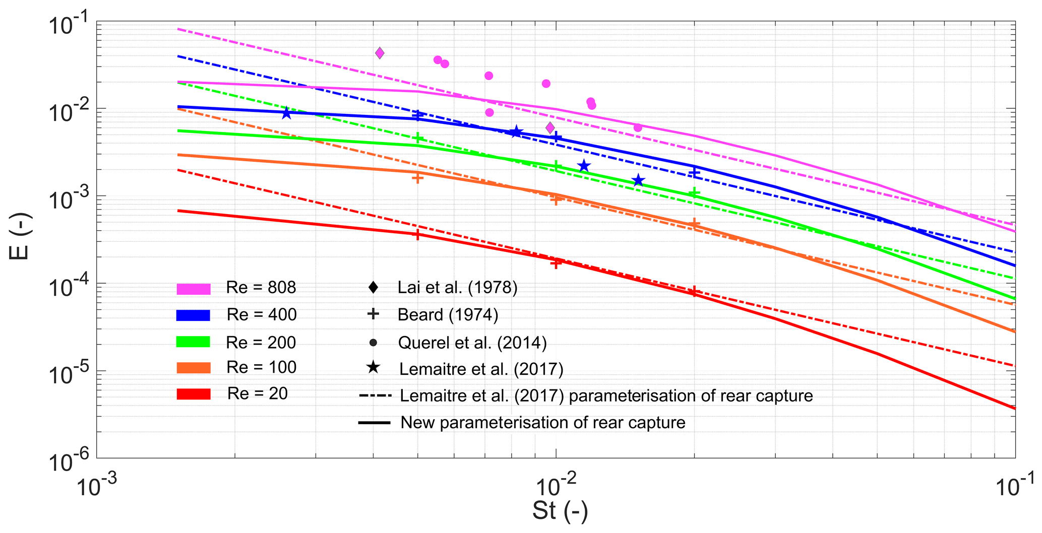
Figure 1 A new parameterisation of the collection efficiency due to rear capture in the raindrop wake. Also plotted are the data used to fit the parameterisation and the original model of Lemaitre et al. (2017).

2.4 Rear capture

Many of the numerical models that were used to develop the semi-empirical relationships between the collection efficiencies and the environmental variables (e.g. Eqs. 6–11) made pragmatic assumptions such that the collector raindrop and collected particle were both spherical and that the flow around the raindrop was Stokes or potential flow (e.g. Slinn, 1984). These assumptions are inaccurate for raindrops with diameters D_d>280 µm, wherein the raindrop becomes oblate and is prone to oscillate, and the surrounding flow is viscous and asymmetric (Quérel et al., 2014). Beard and Grover (1974) and Beard (1974) used a complex numerical model with a more accurate representation of the viscous flow around a raindrop than Slinn (1984) to discern the impact of raindrop-induced vortices on the collection efficiency, albeit still assuming both raindrop and particle to be spherical. They found that for intermediate Reynolds numbers (Re_D) such that $\mathrm{20}\le R{e}_D\le \mathrm{400}$ (equivalent to $\mathrm{280}\le D_{\mathrm{d}}\le \mathrm{1260}$ µm), the rear-capture effect is an important mechanism for aerosol collection. Measurements from Wang and Pruppacher (1977) suggest that for raindrops with D_d>1260 µm, the rear-capture effect progressively decreases.

Recent laboratory studies by Quérel et al. (2014) and Lemaitre et al. (2017) have shone light on the importance of the rear-capture effect. By comparing the results of Slinn (1984) and Beard (1974), Lemaitre et al. (2017) derived a semi-empirical formula for the collection efficiency due to rear capture as a function of Reynolds number, which characterises the flow around the raindrop, and Stokes number (St), which characterises the particle's inertia and susceptibility to capture. This model was valid for Reynolds numbers between $\mathrm{20}\le R{e}_D\le \mathrm{400}$ and for Stokes numbers between $\mathrm{5}\times {\mathrm{10}}^{-\mathrm{3}}\le St\le \mathrm{5}\times {\mathrm{10}}^{-\mathrm{2}}$ (equivalent to $\mathrm{0.3}\le d_{\mathrm{p}}\le \mathrm{1.1}$ µm for $\mathrm{280}\le D_{\mathrm{d}}\le \mathrm{1260}$ µm), which is a rather limited subset of the raindrop and particle diameter spectra. Quérel et al. (2014) found the rear-capture effect to be important up to a Re_D≈800 (D_d≈1910 µm), with the disparity attributed to the assumption of spherical raindrops by Beard (1974). In this paper, a new parameterisation of the collection efficiency via rear capture is presented – fit to a greater range of observations (Fig. 1) – which is applicable to the entire aerosol size spectrum (Eq. 12). Crucially, the new collection efficiency asymptotes to zero with decreasing aerosol diameter, following the logic that nanometre-sized aerosols are more likely to be collected by frontal capture via Brownian diffusion. Equation (12) is applicable for $\mathrm{20}\le R{e}_D\le \mathrm{800}$, while for Re_D outside this range it is pragmatically assumed here that $E_{rc}\left(d_{\mathrm{p}},D_{\mathrm{d}}\right)=\mathrm{0}.$

$$\begin{array}{}\text{(12)}& E_{rc}\left(d_{\mathrm{p}},D_{\mathrm{d}}\right)=\left\{\begin{array}{ll}\frac{\mathrm{1}}{\mathrm{1.37}\times {\mathrm{10}}^{\mathrm{10}}}S{t}^{-\mathrm{3.625}}R{e}_D^{\mathrm{1.444}}\times & \mathrm{20}\le R{e}_D\le \mathrm{800}\\ e^{-\mathrm{0.243}{\left(\ln St\right)}^{\mathrm{2}}}{e}^{\mathrm{0.08144}\left(\ln St\right)\ln R{e}_D}& \\ \mathrm{0}& \mathrm{otherwise}\end{array}\right.\end{array}$$

2.5 Wang et al. (2014) model for Λ

Various studies have suggested that the disparity between observed and modelled BCS rates is mostly attributable to confounding atmospheric processes such as nucleation scavenging, turbulent diffusion, and precipitation-induced downdrafts (e.g. Wang et al., 2010, 2011; Andronache et al., 2006). Wang et al. (2010) in particular recommend that the theoretical BCS models with the greatest values of Λ should be used in GCMs. Given the complexity of such schemes (e.g. Eqs. 6–12 and Sects. S1–S5), it is useful to derive simplified formulae that can reduce the computational cost of explicitly calculating Λ online in a GCM. In answer to this, Wang et al. (2014) fit a simple polynomial formula to the upper 90th percentile of Λ from various theoretical models in the literature as a function of aerosol diameter and rain rate (Eq. 13), that can be used instead of explicitly evaluating Λ using Eq. (2). The coefficients in Eq. (13) are provided in Table 8 in Wang et al. (2014) and Table S2. In Eq. (13), d_p is in units of micrometres (µm) rather than units of metres used elsewhere in this study.

$$\begin{array}{}\text{(13a)}& \mathrm{\Lambda }\left(d_{\mathrm{p}},R\right)=A\left(d_{\mathrm{p}}\right)R^{B\left(d_{\mathrm{p}}\right)}\end{array}$$

$$\begin{array}{}\text{(13b)}& {\log }_{\mathrm{10}}A\left(d_{\mathrm{p}}\right)=\left\{\begin{array}{l}\sum _{i=\mathrm{0}}^{\mathrm{3}}{a}_i{\left({\log }_{\mathrm{10}}{d}_{\mathrm{p}}\right)}^i{d}_{\mathrm{p}}\le \mathrm{2}\mathrm{\mu }\mathrm{m}\\ \sum _{i=\mathrm{0}}^{\mathrm{6}}{b}_i{\left({\log }_{\mathrm{10}}{d}_{\mathrm{p}}\right)}^i{d}_{\mathrm{p}}>\mathrm{2}\mathrm{\mu }\mathrm{m}\end{array}\right.\end{array}$$

$$\begin{array}{}\text{(13c)}& B\left(d_{\mathrm{p}}\right)=\left\{\begin{array}{l}\sum _{i=\mathrm{0}}^{\mathrm{1}}{c}_i{\left({\log }_{\mathrm{10}}{d}_{\mathrm{p}}\right)}^i{d}_{\mathrm{p}}\le \mathrm{2}\mathrm{\mu }\mathrm{m}\\ \sum _{i=\mathrm{0}}^{\mathrm{6}}{e}_i{\left({\log }_{\mathrm{10}}{d}_{\mathrm{p}}\right)}^i{d}_{\mathrm{p}}>\mathrm{2}\mathrm{\mu }\mathrm{m}\end{array}\right.\end{array}$$

2.6 Laakso et al. (2003) model for Λ

Laakso et al. (2003) derived a formula for Λ as a function of aerosol diameter and rainfall intensity, using 6 years of measurements from a boreal forest site in Southern Finland (Eq. 14). Their model is widely used in GCMs but was only fit to a limited range of R and d_p: R≤20 mm h⁻¹ and $\mathrm{0.01}<d_{\mathrm{p}}<\mathrm{0.5}$ µm. However, Fig. 7 in Laakso et al. (2003) shows that the model does an excellent job at capturing observed Λ from Volken and Schumann (1993) for $\mathrm{0.5}<d_{\mathrm{p}}<\mathrm{10}$ µm, albeit for a single value of R. Given the strong gradient in Λ with d_p at d_p=0.5 µm, it seems appropriate to extend this model up to 10 µm with the necessary caveats attached. Outside these range of values (i.e. for R>20 mm h⁻¹, d_p<0.01 µm, and d_p>10 µm) the values at the extrema are used. As with the model proposed by Wang et al. (2014) for Λ, Eq. (14) can be used instead of explicitly evaluating Eq. (2) in the algorithm described in Sect. 2.1. In Eq. (14), d_p is in units of metres, and the coefficients a_i are a₀=274.35758, a₁=332839.59273, a₂=226656.57259, a₃=58005.91340, a₄=6588.38582, and a₅=0.244984.

$$\begin{array}{}\text{(14a)}& {\displaystyle }\mathrm{\Lambda }\left(d_{\mathrm{p}},R\right)& {\displaystyle }={\mathrm{10}}^{A(d_{\mathrm{p}},R)}\text{(14b)}& {\displaystyle }A\left(d_{\mathrm{p}},R\right)& {\displaystyle }=\sum _{i=\mathrm{0}}^{\mathrm{4}}{a}_i{\left({\log }_{\mathrm{10}}{d}_{\mathrm{p}}\right)}^{-i}+a_{\mathrm{5}}{R}^{\mathrm{0.5}}\end{array}$$

3 Box model simulation design

The BCS algorithm as described in Sect. 2, with ${\mathrm{\Lambda }}_N\left(\stackrel{\mathrm{‾}}{d_{\mathrm{p}}},\mathit{\sigma },R\right)$ and ${\mathrm{\Lambda }}_M\left(\stackrel{\mathrm{‾}}{d_{\mathrm{p}}},\mathit{\sigma },R\right)$ tabulated assuming various collection efficiencies and BCS rates (Sect. 2.2–2.6), is first tested in offline box model simulations before being implemented in the UM. The box model simulations use a simple forward Euler time stepping scheme, with 1 min time increments and 180 time steps (or 3 h total duration). Three different rain rates are tested corresponding to drizzle (R=0.5 mm h⁻¹), moderate rain (R=2.5 mm h⁻¹), and heavy rain (R=10 mm h⁻¹). Two initial condition (IC) size distributions are tested: an accumulation mode with ICs of $\stackrel{\mathrm{‾}}{d_{\mathrm{p}}}=\mathrm{0.4}$ µm and σ=1.59 and a coarse mode with ICs of $\stackrel{\mathrm{‾}}{d_{\mathrm{p}}}=\mathrm{2}$ µm and σ=2. The initial IC distributions are idealised and intended to represent standard dust conditions in the accumulation and coarse regimes. The results of the box model simulations and direct comparisons between the BCS rates and collection efficiencies are provided in Sect. 5.1–5.2.

The GLOMAP-mode aerosol model was originally developed as a bin scheme (GLOMAP-bin; Spracklen et al., 2005), with 20 logarithmically spaced size bins spanning 2 nm to 22 µm. In order to test the impact of BCS on the modal width (σ), which relates to KQ4, the offline box model is further run with the GLOMAP-bin size bins, extended upwards by 4 bins to 150 µm. Specifically, the log-normal cumulative distribution function is used to obtain the initial mass and number concentrations in each bin for an initial log-normal distribution. The box model is then integrated over each bin individually, using the geometric mean of the bin thresholds as a representative diameter and the SLINN+PH+RC BCS rates to determine the BCS rate per bin. Finally, log-normal distributions are fit to the bins at T+1 H (1 h elapsed) and T+3H (3 h elapsed) by generating random variables (RVs) from the histograms in Python 3 (Van Rossum and Drake, 2009) and fitting a log-normal distribution to the RVs using maximum likelihood estimation. A comparison of BCS applied to a bin aerosol model and to a modal aerosol model is provided in Sect. 5.2.

4 The Met Office Unified Model configuration and simulation design

4.1 UM configuration (UM-GA8.0)

In order to compare the various BCS schemes outlined in Sect. 2, GCM simulations were performed using the Met Office UM in an atmosphere-only mode with the latest science configurations Global Atmosphere vn8.0 (GA8.0) and Global Land vn9.0 (GL9.0). A technical overview of GA8.0/GL9.0 has not yet been published, but in effect GA8.0/GL9.0 consolidates the changes introduced at GA7.1 (Walters et al., 2019), including the introduction of a cloud droplet spectral dispersion parameterisation based on Liu et al. (2008), near-surface drag improvements (Williams et al., 2020), and multiplicative scaling of DMS emissions (Bodas-Salcedo et al., 2019). Although the UM can be run at various resolutions, the resolution used here is the climate configuration N96L85, i.e. 1.875^∘ longitude by 1.25^∘ latitude, with 85 vertical levels up to a model lid at 80 km, with 50 levels below 18 km altitude and a model time step of 20 min (Walters et al., 2019). The model is technically named after its science configuration (UM-GA8.0), which we adopt in this study.

UM-GA8.0 includes the coupled UKCA-mode aerosol and chemistry scheme which holistically simulates atmospheric composition in the Earth system, with chemistry and aerosols called once per model hour at N96L85 and emissions updated every time step (Archibald et al., 2020). UM-GA8.0 uses a simplified UKCA chemistry configuration, with important oxidants (O₃, OH, NO₃, HO₂) prescribed as monthly mean climatologies (Walters et al., 2019; Mulcahy et al., 2020). UKCA-mode includes a prognostic double-moment aerosol scheme that carries aerosol mass and number concentrations in a predetermined number of log-normal modes spanning nucleation to coarse sizes (Mann et al., 2010; Mulcahy et al., 2020). In its default configuration, UKCA-mode comprises four soluble modes (nucleation, Aitken, accumulation, and coarse), as well an insoluble Aitken mode, with four aerosol constituents represented: sulfate (SO₄), sea salt (SS), black carbon (BC), and organic carbon (OC). Although UM-GA8.0 incorporates the CLASSIC mineral dust scheme by default (Woodward, 2001), we elect to use the inbuilt UKCA-mode dust scheme in this investigation, which comprises externally mixed dust in two insoluble modes (Sect. 4.2).

The direct aerosol radiative effect is treated with UKCA_RADAER, which uses lookup tables of Mie extinction parameters based on size and a volume-mixed refractive index based on speciated ambient aerosol concentrations (Bellouin et al., 2013). Aerosol water content and hygroscopic growth of the soluble modes are simulated prognostically using the Zdanovskii–Stokes–Robinson (ZSR) method.

4.2 UKCA-mode dust and dust emissions scheme

The UKCA-mode dust scheme is mostly unchanged from Mann et al. (2010). Mineral dust is represented by accumulation and coarse insoluble modes with fixed geometric widths of 1.59 and 2 respectively. Functionality exists in UKCA-mode to permit dust ageing into the equivalent soluble modes, from acting as condensation nuclei for soluble vapours or by coagulation with soluble aerosols, but at the present time these processes are not included in our simulations, and dust remains insoluble throughout its atmospheric lifetime. Owing to the assumption of insolubility, dust is not permitted to act as liquid cloud condensation nuclei (CCN) and thus be removed from the atmosphere by nucleation scavenging in these simulations. This is a simplification, as insoluble aerosol can act as CCN according to Köhler theory, albeit at higher relative humidities than for soluble aerosol (Seinfeld and Pandis, 1998).

Dust emissions are determined each time step using a method based on the widely used scheme of Marticorena and Bergametti (1995). Horizontal flux is calculated in nine bins with boundaries at 0.0632, 0.2, 0.632, 2.0, 6.32., 20.0, 63.2, 200.0, 632.0, and 2000.0 µm diameter. Total vertical flux in six bins up to 63.2 µm is derived from total horizontal flux and follows the size distribution of the horizontal flux in bins 1 to 6. The dry threshold friction velocity for each bin is taken from Bagnold (1941), while the effect of soil moisture on emissions is treated according to Fécan et al. (1999). Further detail on the dust emissions scheme is provided in Woodward et al. (2022). Mapping the binned emissions to the UKCA-mode dust scheme requires a degree of pragmatism and trial and error. In previous test bed simulations, an optimal mapping emerged, wherein Bin $\mathrm{2}+\mathrm{1}/\mathrm{2}$ Bin 3 was emitted to the accumulation mode, while $\mathrm{1}/\mathrm{2}$ Bin 3 + Bin 4 + Bin 5 were emitted to the coarse mode (Jones et al., 2021). This mapping is subject to change given ongoing improvements to the dust scheme. Note that both Bin 1 ($\mathrm{0.0632}<d_{\mathrm{p}}<\mathrm{0.2}$ µm) and Bin 6 ($\mathrm{20}<d_{\mathrm{p}}<\mathrm{63.2}$ µm) emissions, which are included in CLASSIC, are missing from UKCA-mode dust, which constitutes a large fraction of the total particle number (Bin 1) and mass (Bin 6) emitted. In future, a third insoluble mode representing giant dust particles (e.g. Ryder et al., 2019) may be added to UKCA-mode to increase the degrees of freedom to 5 in line with CLASSIC and further resolve the span of the emitted dust size distribution, but that is outside the scope of this work.

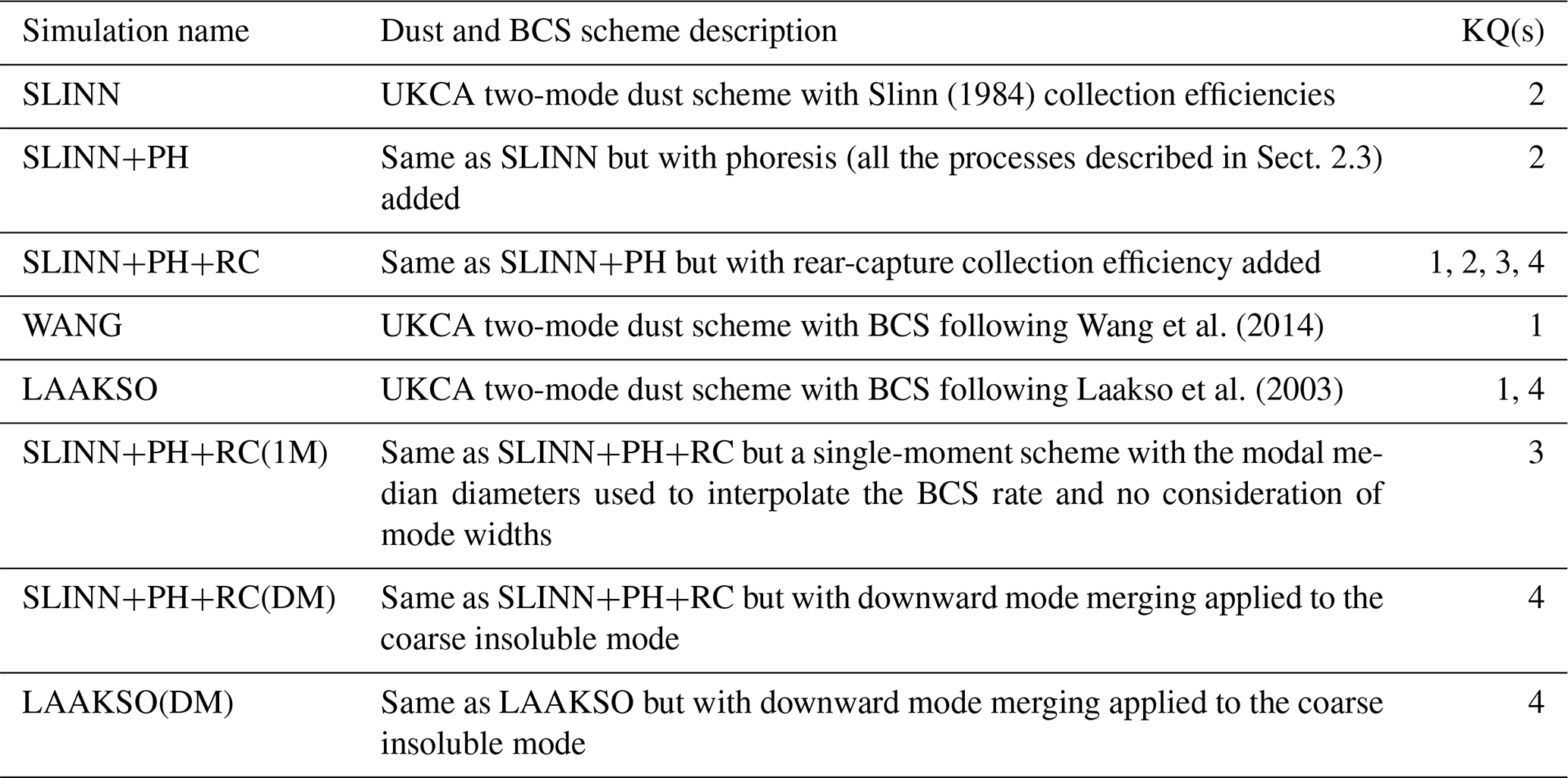
The density of mineral dust is assumed to be invariant at 2650 kg m⁻³ (Mahowald et al., 2014), with refractive indices from Balkanski et al. (2007). Dry deposition and sedimentation in UKCA-mode follow the double-moment resistance type framework outlined by Mann et al. (2010) with sub-time steps of 30 and 15 min for the accumulation and coarse insoluble modes respectively. Downward mode merging (i.e. KQ4; see the Introduction) follows the approach outlined in Mann et al. (2010) for upward mode merging and is initiated when the coarse-mode median diameter falls below the critical threshold of d_p=1 µm, whereupon mass and number are transferred from the coarse insoluble mode to the accumulation insoluble mode. The maximum fraction of the initial number and mass concentration permitted to be transferred per time step is 50 % and 99 % respectively, following UKCA-mode's existing mode-merging protocol. The default UKCA-mode aerosol setup includes upward mode merging for the soluble modes following aerosol growth processes such as cloud processing, coagulation, and condensation but does not represent downward mode merging. Note that only a subset of simulations described here include downward mode merging (see Table 1).

Table 1 Description of the UM-GA8.0 simulations performed and the key questions (KQs) addressed by each simulation.

4.3 UM-GA8.0 simulation design

UM-GA8.0 simulations are performed using standard Atmospheric Model Intercomparison Project (AMIP) protocol. UM-GA8.0 uses CMIP6-defined historical greenhouse gas and aerosol emissions and concentrations fields as detailed by Sellar et al. (2020). Sea-surface temperature and sea-ice fields are fixed time series from the NOAA high-resolution blended analysis of daily sea surface temperature (SST) and ice (OISST V2) reanalysis product (Reynolds et al., 2007) and are updated daily. The simulations are free-running (i.e. not nudged to reanalyses) and are run for 20 model years (1989–2008), with atmospheric mineral dust concentrations initialised to zero. Given the spin-up time necessary for atmospheric dust concentrations to reach equilibrium, only the last 15 model years are used for the analysis.

Table 1 describes the simulations performed for this study, including which key questions or KQs (see Introduction) are pertinent to each simulation. Note that the same nomenclature is adopted for the offline BCS model and box model as for the name of the corresponding UM-GA8.0 simulations except with lowercase and italics. For example, Slinn refers to the BCS scheme proposed by Slinn (1984) (Sect. 2.2), while SLINN refers to the UM-GA8.0 simulation which employs the Slinn BCS model. In addition to testing the various double-moment BCS approaches (Sect. 2.2–2.6), we additionally test the assumption of a single-moment BCS scheme using the Slinn+ph+rc model for Λ in simulation SLINN+PH+RC(1M) and the impact of including downward mode merging in theoretical and empirical BCS models in SLINN+PH+RC(DM) and LAAKSO(DM) respectively. Note that Slinn+ph+rc is the default model used as the basis for answering KQ3 and KQ4 as well as representing theoretical schemes in answering KQ1. The reason Slinn+ph+rc was chosen rather than Slinn, Slinn+ph, Wang, or Laakso is that it fulfils the recommendation by Wang et al. (2010) that the best BCS model to use is the theoretical scheme with the highest BCS rates (see Sect. 5.1). A working hypothesis is then that Slinn+ph+rc most accurately reflects the real-life BCS process of the models tested.

4.4 Validatory observations

A range of observations are employed to test the fidelity of the individual BCS schemes. For seasonal dust optical depth (DOD) at 440 nm, observations are provided by the Aerosol Robotic Network (AERONET; Holben et al., 1998) at eight “dusty” locations from those selected by Bellouin et al. (2005). Also, we use observationally constrained simulated regional 550 nm DODs from Kok et al. (2021), based on Ridley et al. (2016) DOD observations for the Northern Hemisphere and Adebiyi et al. (2020) for the Southern Hemisphere. The criteria imposed for selecting “dusty” AERONET stations are at least 4 years of continuous monthly data with at least 10 daily means per month and an aerosol Ångström exponent (870–440 nm) below 0.5 for at least 10 months of the year. For near-surface dust concentrations, we employ seasonal-mean observations from the historical University of Miami Oceanic Aerosols Network (U-MIAMI) (Prospero and Nees, 1986), which is often used to validate dust models (e.g. Peng et al., 2012; Checa-Garcia et al., 2021). A global network of dust total deposition fluxes (i.e. involving wet and dry deposition processes) is provided by Huneeus et al. (2011). The Kok et al. (2021) DODs, AERONET DODs, and U-MIAMI concentrations are presented in Tables S3, S4, and S5 respectively, whilst the deposition rates are provided in Huneeus et al. (2011).

For the dust particle size distributions (PSDs), which are used to evaluate the impact of representing downward mode merging (Sect. 5.6), observations are compiled from a transatlantic transect of three independent aircraft campaigns: Fennec 2011, representing dust near the source regions of Mali and Mauritania (Ryder et al., 2013); AER-D, representing dust in the Saharan Air Layer (SAL) over the east equatorial Atlantic (Ryder et al., 2018); and the Saharan Aerosol Long-Range Transport and Aerosol–Cloud-Interaction Experiment (SALTRACE) campaign, representing dust over the west equatorial Atlantic (Weinzierl et al., 2017), with additional processing as described in Ryder et al. (2019). We use the campaign mean fitted PSDs presented in Fig. 9 of Ryder et al. (2019) for Fennec 2011 and AER-D, which each comprise a quadrimodal log-normal size distribution with 10th and 90th percentiles. For SALTRACE, we use number size distributions (NSDs) and volume size distributions (VSDs) collected from a single straight and level run during SALTRACE flight 130622a (22 June 2013), alongside 16 % and 84 % percentiles. The PSDs were inferred using the Bayesian inversion algorithm of Walser et al. (2017). The following averaging regions are used to approximately collocate simulated dust concentrations with the observations: (4–8^∘ W, 21–26^∘ N) and 0.1–1.2 km altitude for Fennec 2011 to coincide with the fresh dust observations, (18–24^∘ W, 14–24^∘ N) and 2–3 km altitude for AER-D, and (58–61^∘ W, 11–14^∘ N) and 2–2.4 km altitude for SALTRACE. Temporally, Fennec 2011 and SALTRACE are taken to represent conditions in June and AER-D in August, i.e. the month of operation for each campaign.

5 Results

5.1 Collection efficiencies and BCS rates

Before comparing the BCS schemes in the UM-GA8.0 simulations, it is useful to directly compare collection efficiencies and BCS rates between the models. Given that a new formulation for the “rear-capture” collection efficiency is provided in this paper (Eq. 12), it is also useful to assess if and when rear capture makes an important contribution to the overall collection efficiency. Figure 2 shows the dominant collection efficiency as a function of aerosol diameter and raindrop diameter for the processes outlined in Sect. 2.2–2.4, where by “dominant” we mean the largest collection efficiency numerically determined using the algorithm described in Sect. 2 and standard atmospheric conditions (Table S1). It is clear that rear capture (Rc) makes a substantial contribution to the overall collection efficiency for a large portion of the aerosol and raindrop size spectrum, in particular, in the Greenfield gap for accumulation-sized aerosols and moderate to large raindrop diameters (400 µm–2 mm). Figure 2 also highlights that the Slinn (1984) processes of Brownian diffusion (Br), interception (In), and impaction (Im) only dominate the collection efficiency for a limited size subspace. For aerosol diameters between 0.2–3 µm, rear capture, thermophoresis (Th), and electric charge (Es) are consistently the dominant BCS processes. Note that the contours of the total collection efficiency are discontinuous at $D_{\mathrm{d}}\approx \mathrm{2}\times {\mathrm{10}}^{\mathrm{3}}$ µm in Fig. 2 because this is the upper raindrop diameter for the legitimacy of the formula for E_rc(d_p,D_d) (i.e. Eq. 12), above which E_rc=0.

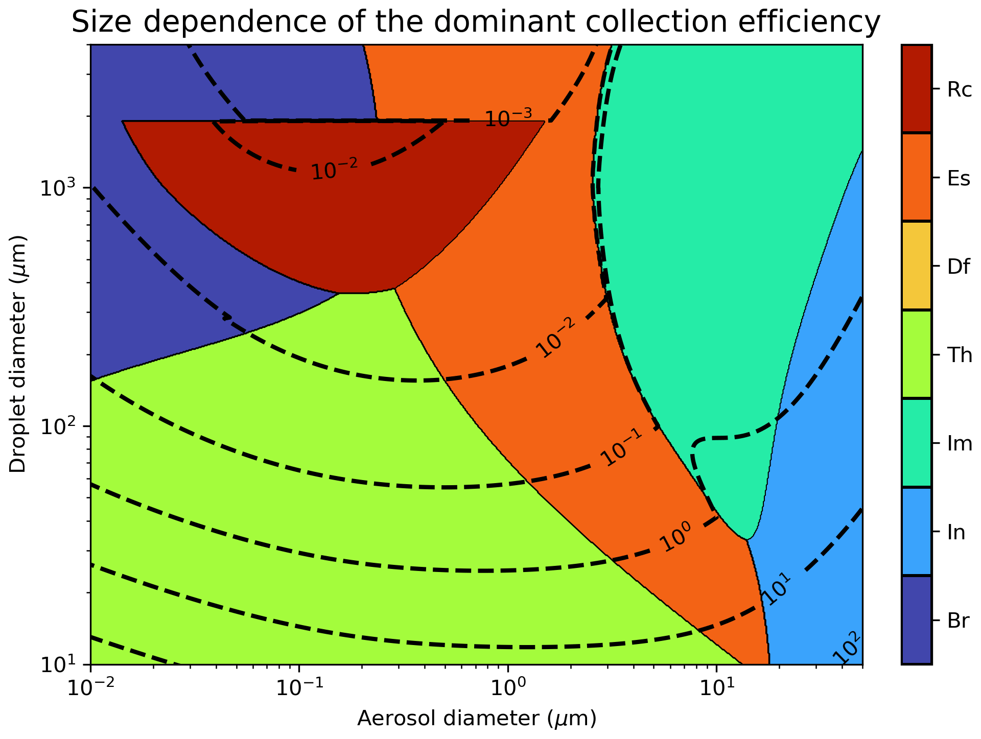
Figure 2 The dominant contributor to the total collection efficiency (i.e. the largest determined numerically) as a function of aerosol diameter and raindrop diameter, where Rc is rear capture, Es is electric charge, Df is diffusiophoresis, Th is thermophoresis, Im is inertial impaction, In is interception, and Br is Brownian diffusion. Dashed lines show logarithmically spaced contours of total collection efficiency.

Figure 3 shows the BCS rate as a function of aerosol diameter and rainfall rate (Λ(d_p,R), or Λ) for the BCS models outlined in Sect. 2, and for three rain rates corresponding to (a) drizzle, (b) moderate rain, and (c) heavy rain. It is clear that in the Greenfield gap the empirically derived Λ (i.e. Laakso) is markedly greater than the theoretical Λ, for example, being an order of magnitude greater than Slinn+ph+rc at d_p=1 µm for all three rain scenarios. It is also clear from comparing Slinn with Slinn+ph and Slinn+ph+rc that phoresis significantly enhances Λ for aerosol with diameters less than ∼2 µm, while rear capture has a significant impact in the Greenfield gap for moderate and heavy rain scenarios. For super-coarse aerosol with d_p>10 µm, all BCS schemes exhibit Λ of the order $\mathrm{1}\times {\mathrm{10}}^{-\mathrm{4}}$ s⁻¹ for drizzle, while the semi-theoretical Wang scheme exhibits greater Λ for heavy rain ($\mathrm{4}\times {\mathrm{10}}^{-\mathrm{3}}$ s⁻¹) than the other models. In general, the Wang BCS rates are similar to Slinn for drizzle and between the Slinn and Slinn+ph rates for moderate rain, which is surprising given that the Wang model was fit to the upper 90th percentile of the existing theoretical BCS rates and thus should be closer to Slinn+ph over the entire rain rate spectrum, although the Wang model also accounted for the variability from raindrop number density and fall velocity formulations (Wang et al., 2014). Although Fig. 3 shows Λ computed using atmospheric properties representative of surface conditions (P=101 325 Pa, T=20 ^∘C, RH = 80 %), we find that using standard atmospheric conditions at 5 km altitude only changes Λ by a factor of 2 at most for Slinn+ph+rc and is thus a second-order impact compared to the deviation in Λ with particle diameter (Fig. S4).

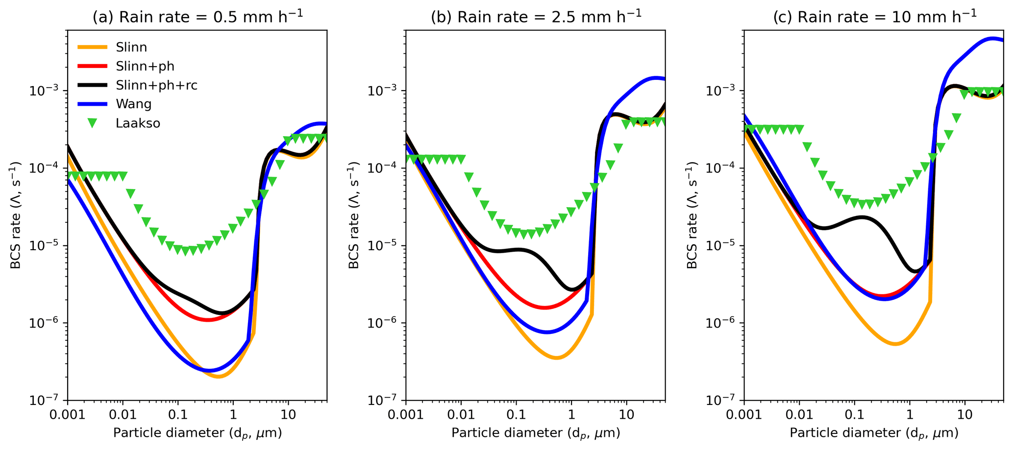
Figure 3 BCS rate (Λ, Eq. 2) as a function of aerosol diameter for five BCS models (Sect. 2) and for rain rates representing (a) drizzle, (b) moderate rain, and (c) heavy rain.

BCS is highly sensitive to aerosol particle size, as shown in Fig. 3. This means that a single-moment BCS scheme which applies the same BCS rate to aerosol number and mass concentrations in a mode, or that does not account for the modal width, may be erroneously simplistic. A single-moment BCS scheme is utilised by UKCA-mode in the UM (Mann et al., 2010), and such is the motivation for KQ3. Figure 4 shows the Slinn+ph+rc BCS rates for monodispersed aerosol ($\mathrm{\Lambda }\left(\stackrel{\mathrm{‾}}{d_{\mathrm{p}}},R\right)$ or Λ; Eq. 2) and for equivalent number and mass distributions (${\mathrm{\Lambda }}_N\left(\stackrel{\mathrm{‾}}{d_{\mathrm{p}}},\mathit{\sigma },R\right)$ and ${\mathrm{\Lambda }}_M\left(\stackrel{\mathrm{‾}}{d_{\mathrm{p}}},\mathit{\sigma },R\right)$ or Λ_N and Λ_M; Eqs. (4) and (5) respectively) assuming geometric widths of σ=1.59 and σ=2, representing the accumulation and coarse insoluble modes in UKCA-mode, respectively. From Fig. 4, it is clear that the effective number and mass BCS rates for log-normal aerosol distribution are significantly greater than the BCS rate for monodispersed aerosols, particularly for $\stackrel{\mathrm{‾}}{d_{\mathrm{p}}}>\mathrm{0.15}$ µm and σ=2. For example, at $\stackrel{\mathrm{‾}}{d_{\mathrm{p}}}\approx \mathrm{1}$ µm, Λ_M is a factor of 150 greater than Λ for all three rain scenarios for σ=2.

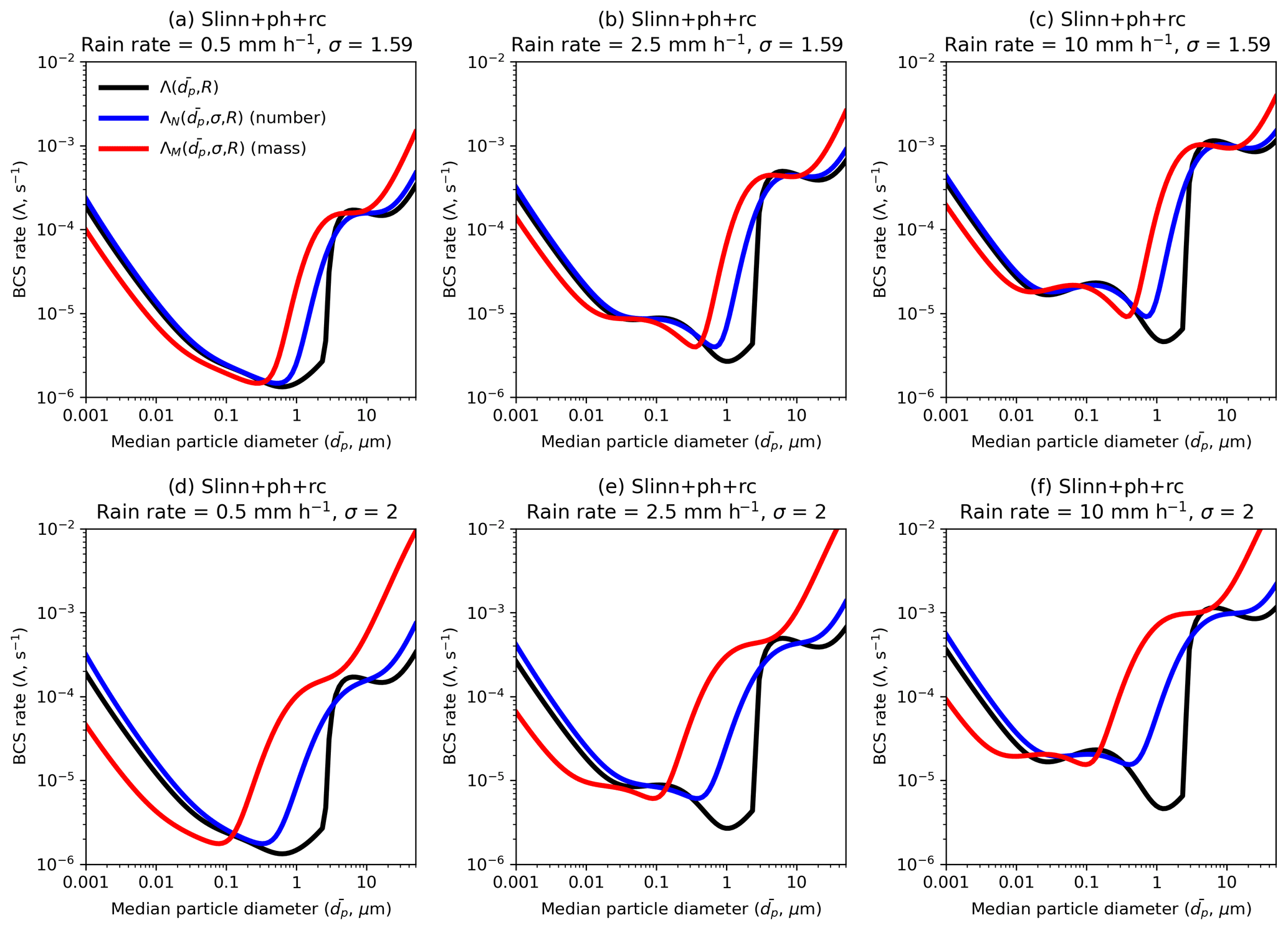
Figure 4 BCS rate integrated over aerosol mass and number (Eqs. 4–5) for geometric widths (a–c) σ=1.59 and (d–f) σ=2, as a function of aerosol diameter for rain rates representing (a, d) drizzle, (b, e) moderate rain, and (c, f) heavy rain.

The change in aerosol median diameter over a time step can be related to the BCS rates Λ_N and Λ_M using Eq. (15) (where $\stackrel{\mathrm{‾}}{d_{p,\mathrm{0}}}$ is the median diameter at the start of the time step, and Δt is the time step in seconds).

$$\begin{array}{}\text{(15)}& \mathrm{\Delta }\stackrel{\mathrm{‾}}{d_{\mathrm{p}}}=\stackrel{\mathrm{‾}}{d_{p,\mathrm{0}}}\left(e^{\frac{\left({\mathrm{\Lambda }}_N-{\mathrm{\Lambda }}_M\right)}{\mathrm{3}}\mathrm{\Delta }t}-\mathrm{1}\right)\left\{\begin{array}{l}\mathrm{\Delta }\stackrel{\mathrm{‾}}{d_{\mathrm{p}}}<\mathrm{0}{\mathrm{\Lambda }}_N<{\mathrm{\Lambda }}_M\\ \mathrm{\Delta }\stackrel{\mathrm{‾}}{d_{\mathrm{p}}}=\mathrm{0}{\mathrm{\Lambda }}_N={\mathrm{\Lambda }}_M\\ \mathrm{\Delta }\stackrel{\mathrm{‾}}{d_{\mathrm{p}}}>\mathrm{0}{\mathrm{\Lambda }}_N>{\mathrm{\Lambda }}_M\end{array}\right.\end{array}$$

Therefore, although both the number and mass concentration decrease each time step, the median diameter may increase, decrease, or remain the same depending on the BCS rates Λ_N and Λ_M and will ultimately converge to a value of d_p such that Λ_N=Λ_M. In Fig. 4d–f, Λ_N and Λ_M are significantly different such that mass is removed faster than number (Λ_N<Λ_M) for $\stackrel{\mathrm{‾}}{d_{\mathrm{p}}}>\mathrm{0.15}$ µm but slower than number (Λ_N>Λ_M) for $\stackrel{\mathrm{‾}}{d_{\mathrm{p}}}<\mathrm{0.15}$ µm, suggesting that, if unaffected by other processes, the aerosol median diameter would converge upon $\stackrel{\mathrm{‾}}{d_{\mathrm{p}}}\approx \mathrm{0.15}$ µm for σ=2 (Fig. 4d–f), i.e. $\stackrel{\mathrm{‾}}{d_{\mathrm{p}}}$ such that Λ_N=Λ_M. For σ=1.59, Λ_N and Λ_M are closer to Λ, and the aerosol median diameter would converge to $\stackrel{\mathrm{‾}}{d_{\mathrm{p}}}\approx \mathrm{0.4}$ µm over time, without accounting for other sink and source processes (Fig. 4a–c).

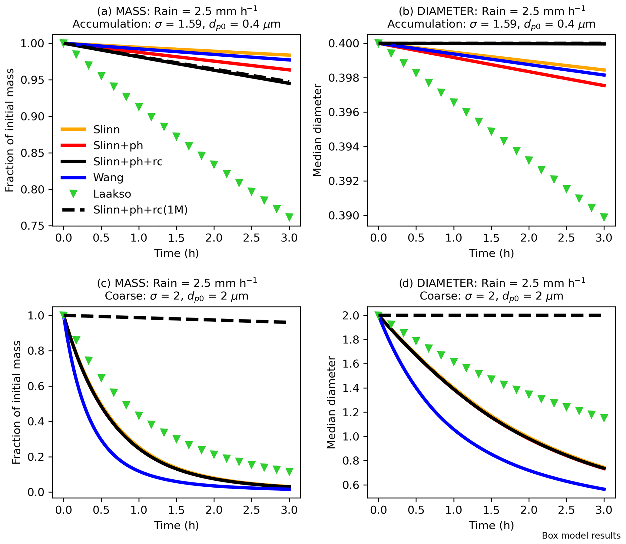
Figure 5 Time evolution of the (a, c) mass concentration and (b, d) median diameter of (a–b) an accumulation-like mode and (c–d) a coarse-like mode with a constant rain rate of 2.5 mm h⁻¹ for six BCS schemes (see Table 1 for definitions). Results from offline box model simulations.

5.2 Box model results

Before comparing the BCS schemes in a GCM environment, it is useful to compare them in a simple offline box model. Figure 5 shows the time evolution of mass and diameter from box model simulations with each of the BCS schemes, assuming a constant rain rate of 2.5 mm h⁻¹ (results for rain rates of 0.5 and 10 mm h⁻¹ are shown in Fig. S5) and for accumulation and coarse aerosol size modes. Note that all results presented in the section are sensitive to the initial conditions for the two modes, and different initial conditions may produce markedly different results given the wide range of Λ, Λ_N, and Λ_M (Figs. 3–4). It is clear that for these initial conditions, there is little deviation in median diameter for the accumulation mode (Fig. 5b) over the 3 model hours for any BCS scheme. However, 2 % of accumulation-mode mass is removed by the end of the simulation in Slinn, compared to 4 % in Slinn+ph and 6 % in Slinn+ph+rc (Fig. 5a), which shows that there is some sensitivity to the additional processes missing in Slinn (KQ2). These differences are small compared to the Laakso scheme, which exhibits a 24 % decrease in accumulation-mode mass over the 3 h duration (KQ1).

For the coarse mode, 97 % of mass is removed over the course of 3 h in the two-moment Slinn and Wang models, and 88 % of mass is removed in Laakso (Fig. 5c). Additionally, the median diameter evolves from $\stackrel{\mathrm{‾}}{d_{\mathrm{p}}}=\mathrm{2}$ µm at the start of the simulation to approximately $\stackrel{\mathrm{‾}}{d_{\mathrm{p}}}=\mathrm{0.75}$ µm in the two-moment Slinn models, $\stackrel{\mathrm{‾}}{d_{\mathrm{p}}}=\mathrm{0.56}$ µm in Wang, and $\stackrel{\mathrm{‾}}{d_{\mathrm{p}}}=\mathrm{1.15}$ µm in Laakso (Fig. 5d). Figure. 5c and d also show the significant impact of using a single-moment BCS scheme, notably that without consideration for the mode width or for the time evolution of $\stackrel{\mathrm{‾}}{d_{\mathrm{p}}}$, only 4 % of coarse-mode mass is removed in the single-moment Slinn+ph+rc(1M) model compared to 97 % in Slinn+ph+rc (Fig. 5c) (KQ3). The difference in mass evolution between Slinn+ph+rc and Slinn+ph+rc(1M) can be attributed to the large difference in mass and uniform BCS rates for $\stackrel{\mathrm{‾}}{d_{\mathrm{p}}}\approx \mathrm{2}$ µm (Fig. 4e). For the accumulation mode, the mass and uniform BCS rates are similar for $\stackrel{\mathrm{‾}}{d_{\mathrm{p}}}=\mathrm{0.4}$ µm in Fig. 4b, hence explaining why there is little difference in accumulation-mode mass evolution between Slinn+ph+rc and Slinn+ph+rc(1M) in the box model simulations (Fig. 5a). Differences between the single-moment and double-moment approaches are explored in Sect. 5.5 using UM-GA8.0.

The BCS results shown so far have assumed a fixed width for the aerosol size distribution, in line with double-moment modal models that are widely employed in GCMs (Gliß et al., 2021). A more advanced but computationally expensive approach is to apportion aerosol mass or number into several fixed-size bins, which increases the degrees of freedom and allows the width of the aerosol mode to evolve. The BCS box model has also been applied to a bin aerosol scheme (see Sect. 3 for Methods), assuming the same initial conditions as for the modal aerosol scheme, with the time evolution of the aerosol number density as a function of aerosol diameter shown in Fig. 6. It is clear from Fig. 6c that aerosol number is more efficiently removed from the coarse bins (d_p>2 µm) than for the smaller bins (d_p<2 µm) when the initial conditions are $\stackrel{\mathrm{‾}}{d_{\mathrm{p}}}=\mathrm{2}$ µm and σ=2 and thus that the effective width of the binned model decreases to σ=1.69 over the course of the 3 h simulation. Conversely, the width is not permitted to shrink in the modal model, and thus the particle number density ($dN/d\log \left(d_{\mathrm{p}}\right))$ for d_p<2 µm is artificially enhanced by the end of the simulation (Fig. 6d). One potential way to compensate for this effect is to introduce downward mode merging (KQ4), whereupon dust mass and number are moved from the broad coarse mode to the narrow accumulation mode following BCS if the new coarse-mode median diameter descends below a threshold value. Downward mode merging is explored in Sect. 4.6 using UM-GA8.0 with the critical threshold value chosen to be 1 µm.

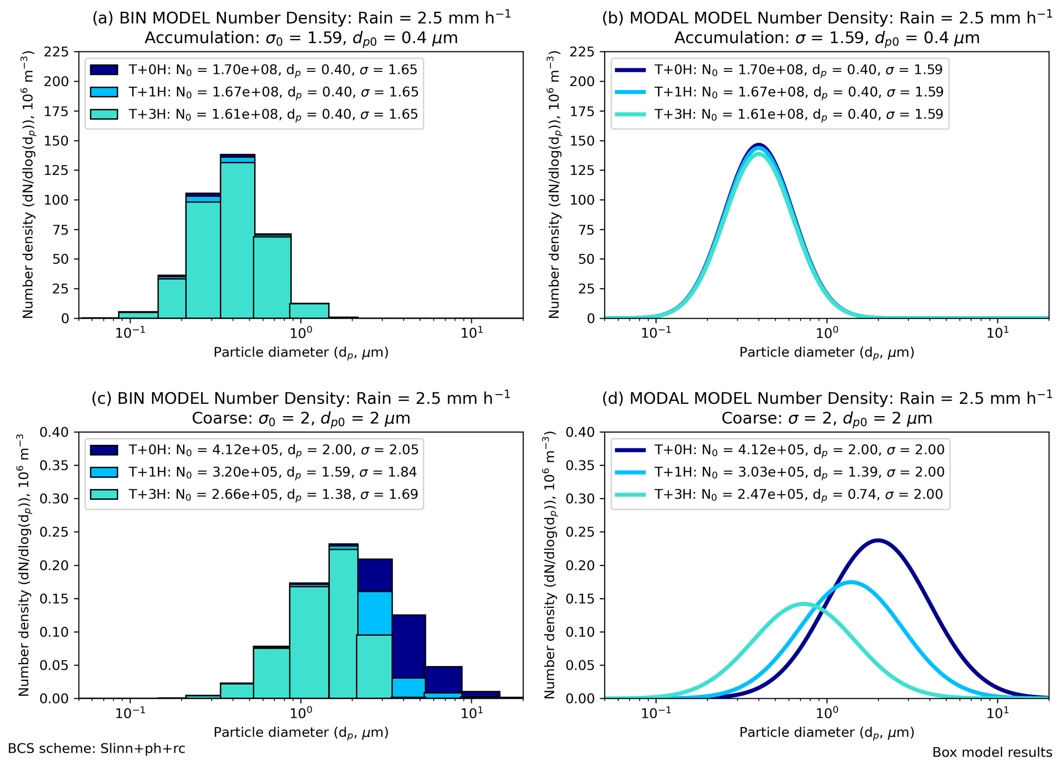
Figure 6 Number density as a function of particle diameter in (a, c) “bin” and (b, d) “modal” simulations with the offline box model. The BCS scheme is Slinn+ph+rc, the rain rate is 2.5 mm h⁻¹, and results are shown for (a–b) an accumulation size distribution and (c–d) a coarse size distribution. The key shows approximate log-normal distributions at T+0H, T+1H, and T+3 H time intervals.

5.3 KQ1: Empirical vs. theoretical BCS schemes

We now move to comparing the BCS schemes in the UM-GA8.0 simulations and thus answering the KQs posed in the Introduction. In order to answer KQ1, the SLINN+PH+RC, WANG, and LAAKSO simulations are compared in terms of global dust metrics. SLINN+PH+RC is chosen over SLINN and SLINN+PH to represent a simulation with a theoretical BCS scheme as it resolves more BCS processes. WANG can be thought of as representing a semi-empirical BCS scheme and has the advantage that it much simpler to compute BCS rates using the Wang model than the Slinn+ph+rc model. LAAKSO represents an entirely empirical BCS scheme. Table 2 shows global dust metrics from all of the UM-GA8.0 simulations performed in this study. From Table 2, it is clear that the order of magnitude difference between the empirical (LAAKSO) and theoretical (SLINN+PH+RC) BCS rates for accumulation-sized aerosol has significant impact on the global dust mass burden. For example, the global accumulation dust burden in LAAKSO is 1.11 Tg, while in SLINN+PH+RC it is 4.61 Tg, and in WANG it is 8.24 Tg. It is clear that BCS is significantly greater in LAAKSO, with 89 % of accumulation dust removed by wet deposition compared to only 72 % in SLINN+PH+RC and 52 % in WANG. Interestingly, accumulation dust emissions are also enhanced by 5 % in LAAKSO compared to the other models, which can only emanate from a change to meteorology, either in terms of soil moisture, surface roughness, or near-surface wind speeds in the dust source regions.

Table 2 Global dust metrics split by mode (accumulation/coarse) for all of the simulations performed in this study.

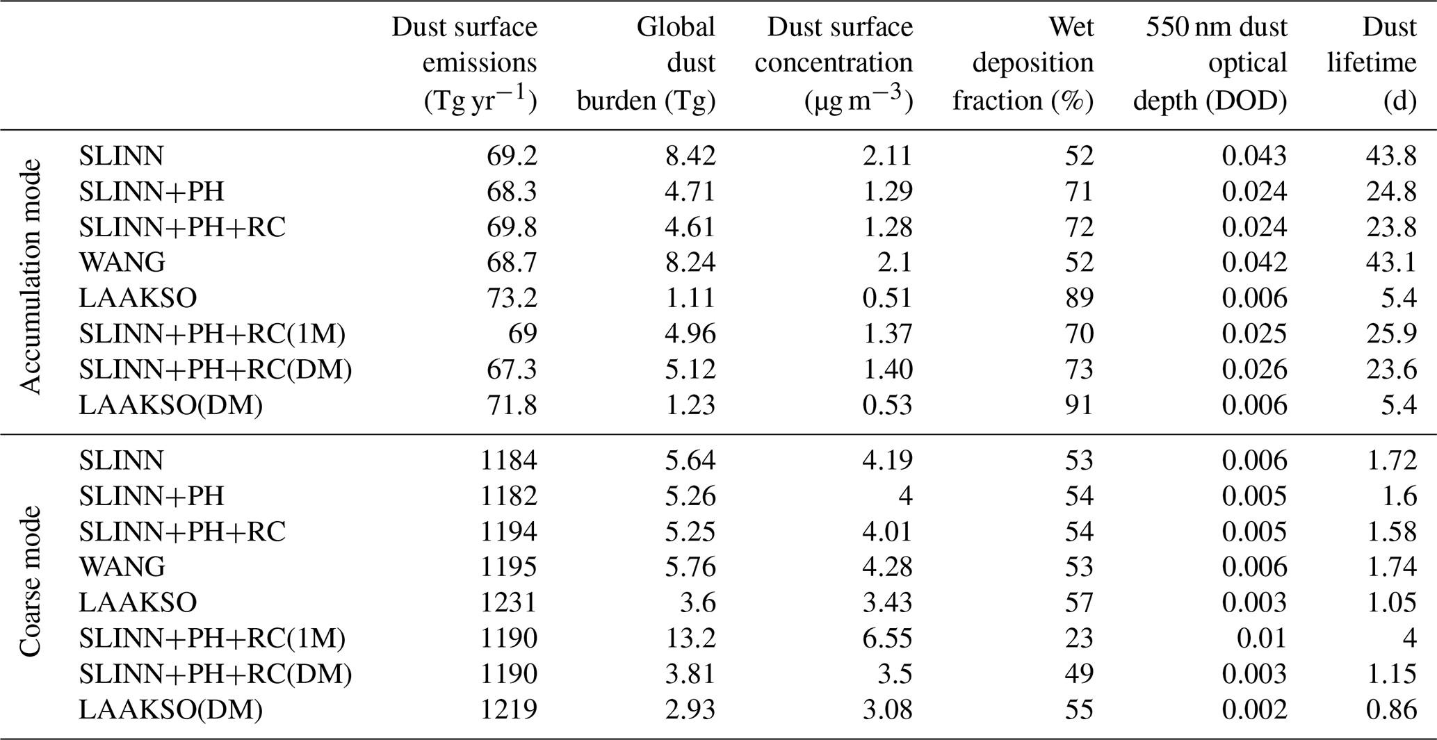
A similar pattern emerges for the coarse mode, with ∼30 % less coarse dust burden in LAAKSO than in SLINN+PH+RC (3.6 Tg compared to 5.25 Tg), owing to the greater BCS rates for $\mathrm{1}\le d_{\mathrm{p}}\le \mathrm{2}$ µm in LAAKSO (Fig. 3). The total dust burden is 53 % less in LAAKSO compared to SLINN+PH+RC (4.7 compared to 9.9 Tg), while DOD is 70 % smaller in LAAKSO than in SLINN+PH+RC (0.009 compared to 0.029). For perspective, the SLINN+PH+RC global-mean total DOD of 0.029 is commensurate to the AeroCom phase 1 mean DOD of 0.029, the intermodel mean DOD from Kok et al. (2021) of 0.028, the mean DOD from most of the CRESCENDO models (Checa-Garcia et al., 2021), and the observationally constrained range of 0.02–0.035 from Ridley et al. (2016). The total dust lifetime is 2.8 d in SLINN+PH+RC, 1.3 d in LAAKSO, and 4 d in WANG, which can be compared to a multimodel mean of 2.5 (±1.3) d in the CRESCENDO models (Checa-Garcia et al., 2021). This tentatively suggests that the SLINN+PH+RC dust metrics are closest to other state-of-the art climate models and observations, whilst LAAKSO may underestimate the longevity of dust in the atmosphere, and WANG may overestimate it. However, a range of caveats limits the extent to which we can say one BCS model is superior to another (see Sect. 6).

Figure 7 shows a comprehensive range of dust metrics for the SLINN+PH+RC, WANG, and LAAKSO simulations, including spatial maps of annual mean dust burden (Fig. 7a–c); seasonal DODs against observationally constrained simulated DOD from Kok et al. (2021) (circles) and observations from AERONET (pluses) (Fig. 7d–f); seasonal near-surface dust concentrations against U-MIAMI observations (Fig. 7g–i); and annual dust deposition against observations compiled by Huneeus et al. (2011) (Fig. 7j–l). The scatter plots (Fig. 7d–l) are supplemented by three statistical measures of predictive skill: the mean correlation coefficient (r), the mean bias, and the root mean square error (RMSE), all of which are calculated in logarithmic (base 10) space, owing to the measurements ranging over many orders of magnitude. These statistics are meant to complement the figures and illustrate the closeness of fit between the model and observations but do not necessarily show which BCS model is best owing to compensating errors and other caveats (see Sect. 6). Spatial plots of annual-mean values for each of the four observation datasets are shown in Fig. S6. It is clear from all of the observational datasets in Fig. S6 that dust is prevalent over source regions in north and equatorial Africa, the Middle East, and Asia and less prevalent over the Americas, Southern Africa, much of the Pacific Ocean, and the poles. In Figs. 7, 8, 9, 11, and S11 we have grouped the observations by region, with associated abbreviations provided in the captions for Tables S3–S5.

Dust is widely distributed over the Earth in WANG, with the greatest burden in the Northern Hemisphere (NH) but substantial concentrations in the Southern Hemisphere (SH) (Fig. 7b). Conversely, dust is almost entirely confined to the NH in LAAKSO, with only source regions in Southern Africa, South America, and Australia (Fig. S7) exhibiting substantial dust burdens in the SH (Fig. 7c). Dust burdens in SLINN+PH+RC are intermediate between LAAKSO and WANG. Simulated DOD in LAAKSO is vastly less than both AERONET observations and Kok et al. (2021) observationally constrained DOD, particularly over secondary source regions such as South America, Southern Africa, and Australia (SAm, SAf, and Aus respectively in Fig. 7d–f). Furthermore, dust concentrations away from source regions such as over the Pacific and Southern oceans (Pac and SOc respectively in Fig. 7i) and deposition rates over the Pacific Ocean (EPac; Fig. 7l) are significantly less in LAAKSO than in the observations, which may imply that the LAAKSO BCS scheme is removing dust too efficiently from the atmosphere near to source regions. Conversely, WANG appears to overestimate dust away from source regions (e.g. Pac in Fig. 7h), despite all models exhibiting too little dust over source regions such as the Sahara, which is reflected in uniformly negative DOD biases relative to AERONET (ANet in Fig. 7d–f). Underestimating Saharan dust emissions (or at least, DOD) appears to be a persistent problem in Met Office Hadley Centre climate models (Mulcahy et al., 2018) and will be exacerbated here by the fact that the largest and smallest dust bins in the existing dust scheme (CLASSIC) are not resolved in UKCA dust.

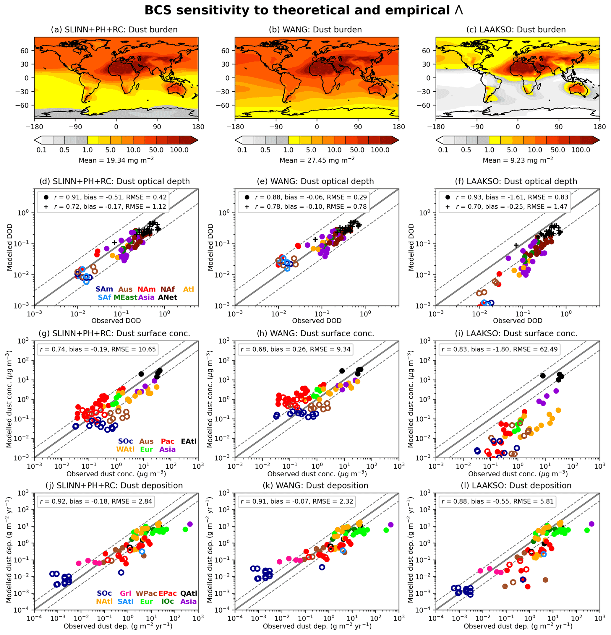
Figure 7 Global dust metrics in the SLINN+PH+RC, WANG, and LAAKSO simulations, used to answer KQ1 – empirical vs. theoretical BCS schemes. (a–c) Annual-mean total dust burden, (d–f) seasonal and regional dust optical depths (DOD) against 440 n nm AERONET observations (+) and 550 nm DODs from Kok et al. (2021), (g–i) seasonal and regional near surface dust concentrations against U-MIAMI observations (Prospero and Nees, 1986), and (j–l) annual-mean regional dust deposition rates against observations from Huneeus et al. (2011). Filled and unfilled circles refer to Northern and Southern Hemisphere measurements respectively. Colours in (d–l) denote different regions, with abbreviations provided in Tables S3–S4 for (d–f) and Table S5 for (g–i). For (j–l), the abbreviations are as follows: SOc – Southern Ocean, Grl – Greenland, WPac – west Pacific Ocean, EPac – east Pacific Ocean, QAtl – equatorial Atlantic Ocean, NAtl – North Atlantic Ocean, SAtl – South Atlantic Ocean, Eur – Europe, and IOc – Indian Ocean.

The WANG simulation exhibits the smallest bias and RMSE in all the metrics (Fig. 7). However, this is partly due to positive biases away from source regions (e.g. over North America, NAm, in Fig. 7e) offsetting negative biases closer to dust source regions (e.g. North Africa, NAf, in Fig. 7e). The SLINN+PH+RC simulation exhibits a good spread about the 1:1 line in terms of comparing simulated DOD and dust concentrations with observations, albeit with a slight overall negative bias (Fig. 7d, g), which may emanate from insufficient dust emissions. However, dust deposition rates over the Southern Ocean (SOc; Fig. 7j) are somewhat overestimated in SLINN+PH+RC, which may emanate from spuriously elevated dust emissions in Australia and Southern Africa, as also exhibited by UKESM (Checa-Garcia et al., 2021), although note that the dust emissions scheme differ somewhat between UKESM and UM-GA8.0 (Woodward et al., 2022). Given the many facets of the dust scheme which may contribute to dust distribution biases, such as deficiencies in emissions and dry deposition rates and precipitation biases, it is impossible to pronounce value judgement on which BCS scheme is best from these simulations. However, it is possible to conclude that dust spatial distributions are highly sensitive to the choice of BCS scheme, with LAAKSO removing dust much more efficiently than SLINN+PH+RC or WANG and closer to source regions (Fig. S8).

5.4 KQ2: Importance of missing processes in the Slinn (1984) BCS model

Figure 8 shows the same dust metrics as in Fig. 7 but plotted for the UM-GA8.0 simulations based on the Slinn (1984) BCS scheme, with and without the missing processes of phoresis and rear capture. The global dust burden is significantly greater in SLINN (27.6 mg m⁻²) than in SLINN+PH (19.5 mg m⁻²) or SLINN+PH+RC (19.3 mg m⁻²), which is mostly driven by an enhanced accumulation-mode dust burden (Table 1). As accumulation-mode aerosol is more optically active in the visible shortwave spectrum than the coarse mode, this results in a reduced DOD bias in SLINN (−0.06; Fig. 8d) compared to SLINN+PH (−0.49; Fig. 8e), or SLINN+PH+RC (−0.51; Fig. 8f). However, dust concentrations away from source regions are greater in SLINN than in the observations (e.g. Pacific, PAc; Fig. 8g), and the positive bias in dust deposition rate over the Southern Ocean is also exacerbated in SLINN (SOc; Fig. 8j), suggesting that the BCS rates may be too low in that model. Other confounding factors affect the atmospheric transport of the dust, such as dry deposition, particle shape, and in-cloud scavenging, and so it is impossible to definitely say that the BCS rates in SLINN are wrong, only that dust is removed less efficiently by BCS in that model, which logically follows from the differences in BCS rates (Fig. 3).

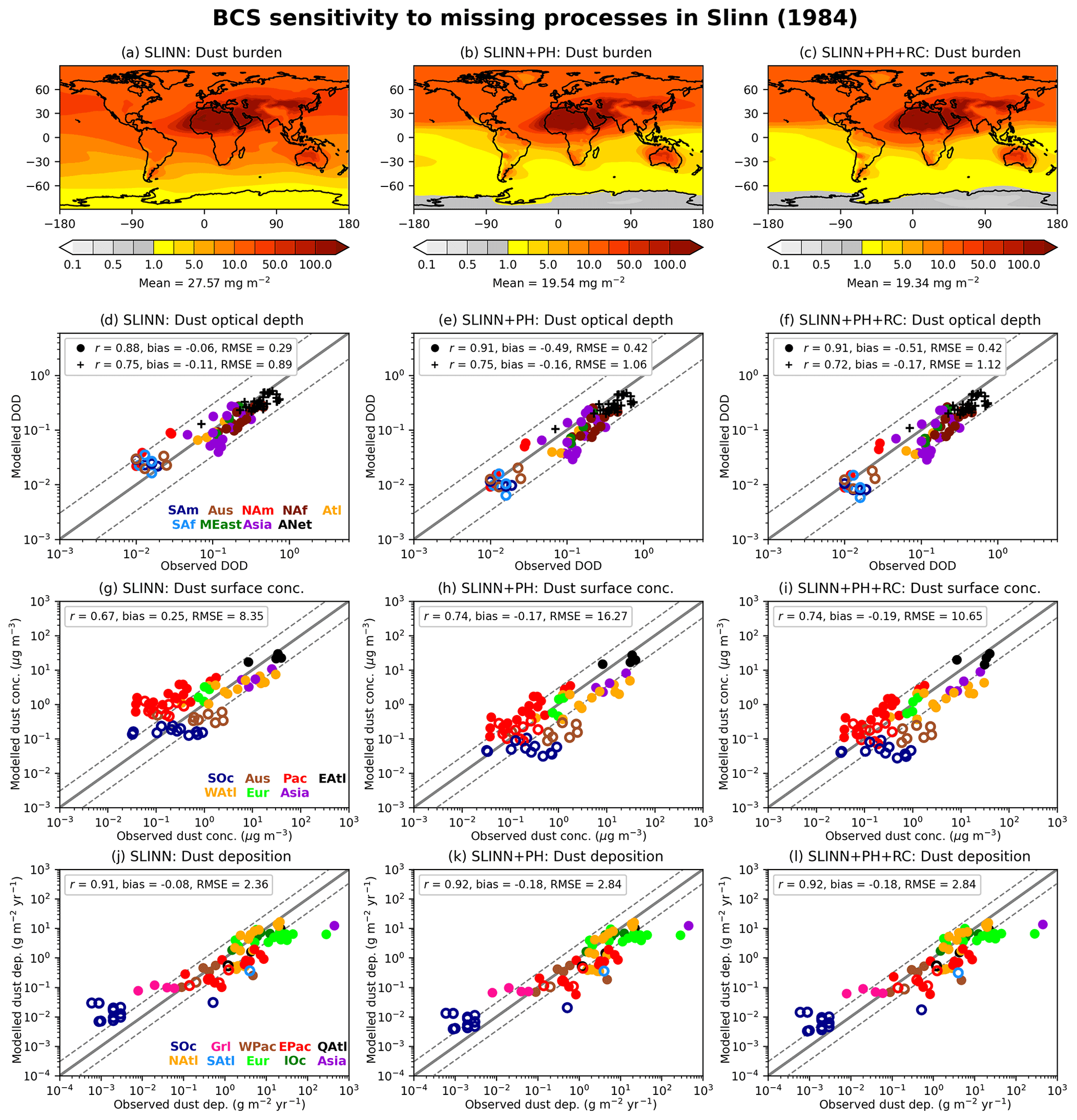
Figure 8 The same as Fig. 7 but for SLINN, SLINN+PH, and SLINN+PH+RC simulations and used to answer KQ2, the impact of missing processes in the Slinn (1984) BCS algorithm.

From Fig. 8, it is clear that phoresis has a significant impact on simulated dust concentrations, particularly in the removal of accumulation-mode aerosol. The addition of rear capture to the model has a smaller impact in the UM-GA8.0 simulations than the addition of phoresis. However, GCMs are unable to resolve heavy precipitation episodes owing to their coarse spatio-temporal resolution (Frei et al., 2006) and are beset with annual and seasonal precipitation biases. For instance, the previous-generation Met Office Hadley Centre climate model (UM-GA7.0) exhibited negative annual-mean precipitation biases over the Indian subcontinent and in general overestimated precipitation over the oceans (Walters et al., 2019), with many of the precipitation issues unrectified in UM-GA8.0 (Fig. S9). Given that the rear-capture effect increases in magnitude non-linearly with precipitation intensity (Fig. 3), it is likely rear capture plays a more important role in wet removal of accumulation-mode dust than exhibited in these simulations, a hypothesis which could be tested using a higher-resolution climate model or a numerical weather prediction (NWP) model. Additionally, precipitation biases will feed through to the dust metrics in Fig. 8, which again reduces our ability to bestow value judgement on the various SLINN schemes other than to rank them in terms of dust removal rates. It is clear from Fig. 8 that models using the Slinn (1984) BCS scheme without consideration for phoresis and to a lesser extent rear capture may be significantly underestimating wet removal of aerosol.

5.5 KQ3: Single-moment vs. double-moment BCS schemes

A double-moment BCS scheme, wherein separate BCS rates are applied to the zeroth (number) and third (mass) moments of the aerosol size distribution accounting for the width of the aerosol mode, will differ most from a single-moment BCS scheme wherever the number and mass BCS rates differ most from the uniform BCS rate (Fig. 4). All of the UM-GA8.0 simulations apart from SLINN+PH+RC(1M) employ a double-moment BCS approach for mineral dust (Table 1). SLINN+PH+RC(1M) instead uses the Slinn+ph+rc BCS model as in SLINN+PH+RC but applies uniform BCS rates (Λ) to both number and mass concentrations rather than number (Λ_N) and mass (Λ_M) BCS rates separately. Because of this, the mineral dust size distributions are not permitted to evolve following BCS in SLINN+PH+RC(1M), which is the same approach used in the default UKCA BCS scheme (applied to all aerosols).

From Figs. 3–4, it is expected that the wider coarse mode (σ=2) would be more affected by the double-moment approach compared to the single-moment approach than the narrower accumulation mode (σ=1.59), owing to the greater mode width and the fact that the accumulation mode covers the range of particle spectrum where the overall BCS rates are less sensitive to particle size, which proves to be the case in the UM-GA8.0 simulations. Nevertheless, the accumulation dust burden is 7.5 % greater in SLINN+PH+RC(1M) than in SLINN+PH+RC (Table 1), and the lifetime of the dust aerosol is 2 d greater in SLINN+PH+RC(1M) than in SLINN+PH+RC (26 compared to 24 d). Thus, the impact of using a double-moment approach on accumulation-mode aerosol should not be discounted. The impact on the coarse mode is more pronounced, with the dust lifetime increasing from 1.6 d in SLINN+PH+RC to 4 d in SLINN+PH+RC(1M), resulting in a factor of 2.5 increase to coarse-mode dust burden in SLINN+PH+RC(1M) (Table 2).

Figure 9 shows the same global and seasonal dust metrics for the SLINN+PH+RC,SLINN+PH+RC(1M), and SLINN+PH+RC(DM) simulations as in Figs. 7 and 8. Interestingly many of the statistical measures of skill relative to the observations are better in the SLINN+PH+RC(1M) simulation than in SLINN+PH+RC; for example, for surface concentrations, the RMSE is significantly less in SLINN+PH+RC(1M) (6.17 compared to 10.65 in SLINN+PH+RC), and negative DOD biases are also reduced. This is rather surprising, given that the double-moment scheme is more physically plausible than the simple single-moment approach, and again highlights the sensitivity of aerosol schemes in GCMs to many interwoven processes such as size distribution assumptions, emissions, sedimentation, and underlying meteorological biases. Like WANG (Fig. 7) and SLINN (Fig. 8), SLINN+PH+RC(1M) exhibits too much dust deposition over the Southern Ocean (SOc; Fig. 9k), which may be attributable to positive dust emission biases in regions such as Australia, South America, and Southern Africa such as seen in UKESM1 (although note that the dust emission schemes are not precisely the same between UKESM1 and UM-GA8.0; Checa-Garcia et al., 2021) and to inefficient wet removal rates in SLINN+PH+RC(1M). Over dust source regions such as the Sahara, negative biases in DOD (ANet and NAf; Fig. 9d) and surface concentrations (east Atlantic, EAtl; Fig. 9g) in SLINN+PH+RC are significantly reduced in SLINN+PH+RC(1M) (Fig. 9e and h respectively), but this again may be an artefact of compensating errors, namely inefficient wet removal of dust and inaccurate dust emissions or representative size distribution. For instance, Mulcahy et al. (2018) found a low DOD bias over the Sahara in simulations with UM-GA8.0 and UKESM1. Thus, a qualified answer to key question 3 is that the double-moment approach does have a significant impact on simulated dust concentrations compared to a single-moment approach, in particular enhancing wet removal rates of the wide coarse-mode aerosol.

5.6 KQ4: Impacts of representing downward mode merging

The downward mode-merging scheme applied in SLINN+PH+RC(DM) and LAAKSO(DM) redistributes aerosol mass and number from the coarse insoluble mode to the accumulation insoluble mode when the coarse-mode median diameter falls below a fixed diameter threshold, in this case d_p=1 µm (Mann et al., 2010). Recall that mode merging is used to artificially represent the contraction of the coarse mode due to size-dependent loss processes such as BCS (i.e. Fig. 6) or sedimentation, which is difficult in models with fixed modal widths. In particular, the “sedimentation-driven” downward merging will happen nearer sources, and one result of it will be that the size distribution of the dust which reaches the area where BCS occurs will be changed from the control experiments. The total mass transferred from the coarse to the accumulation mode is 10.8 Tg yr⁻¹ in SLINN+PH+RC(DM) and 9.8 Tg yr⁻¹ in LAAKSO(DM) or 0.9 % and 0.8 % of the primary coarse dust emissions respectively. Most of the mode merging takes place near to sources regions over the Sahara, Middle East, and East Asian deserts and within 3–5 km of the surface (Fig. S10). The coarse dust lifetime is reduced from 1.58 d in SLINN+PH+RC to 1.15 d in SLINN+PH+RC(DM) and 1.05 d in LAAKSO to 0.86 d in LAAKSO(DM). Concomitantly, the coarse dust burden decreases by 27 % in SLINN+PH+RC(DM) compared to SLINN+PH+RC and 19 % in LAAKSO(DM) compared to LAAKSO, with corresponding increases in accumulation burden in the downward mode-merging simulations (Table 1).

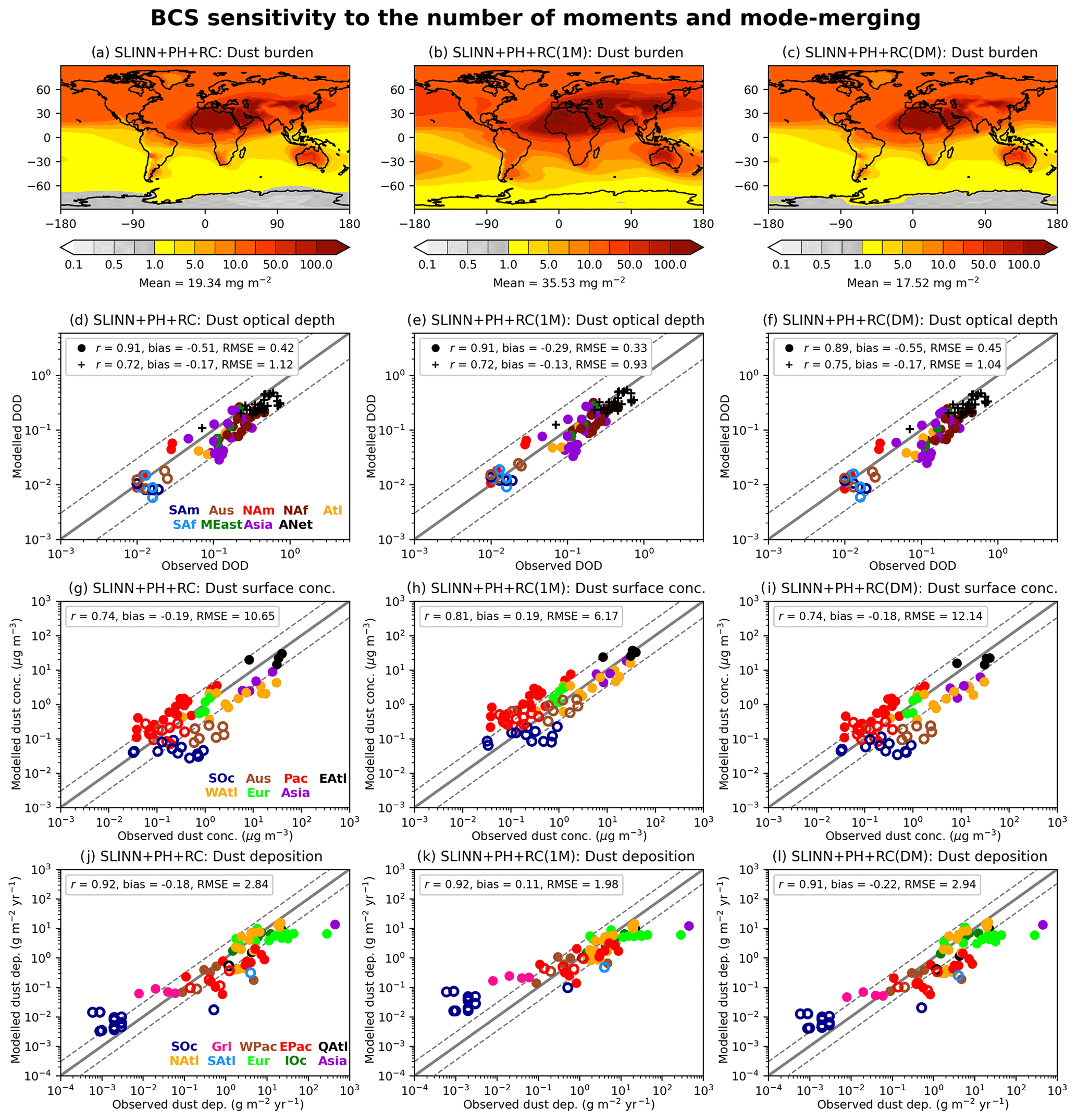
Figure 9 The same as Figs. 7–8 but for SLINN+PH+RC, SLINN+PH+RC(1M), and SLINN+PH+RC(DM). Used to answer KQ3, single- vs. double-moment BCS schemes, and KQ4, impact of representing downward mode merging.

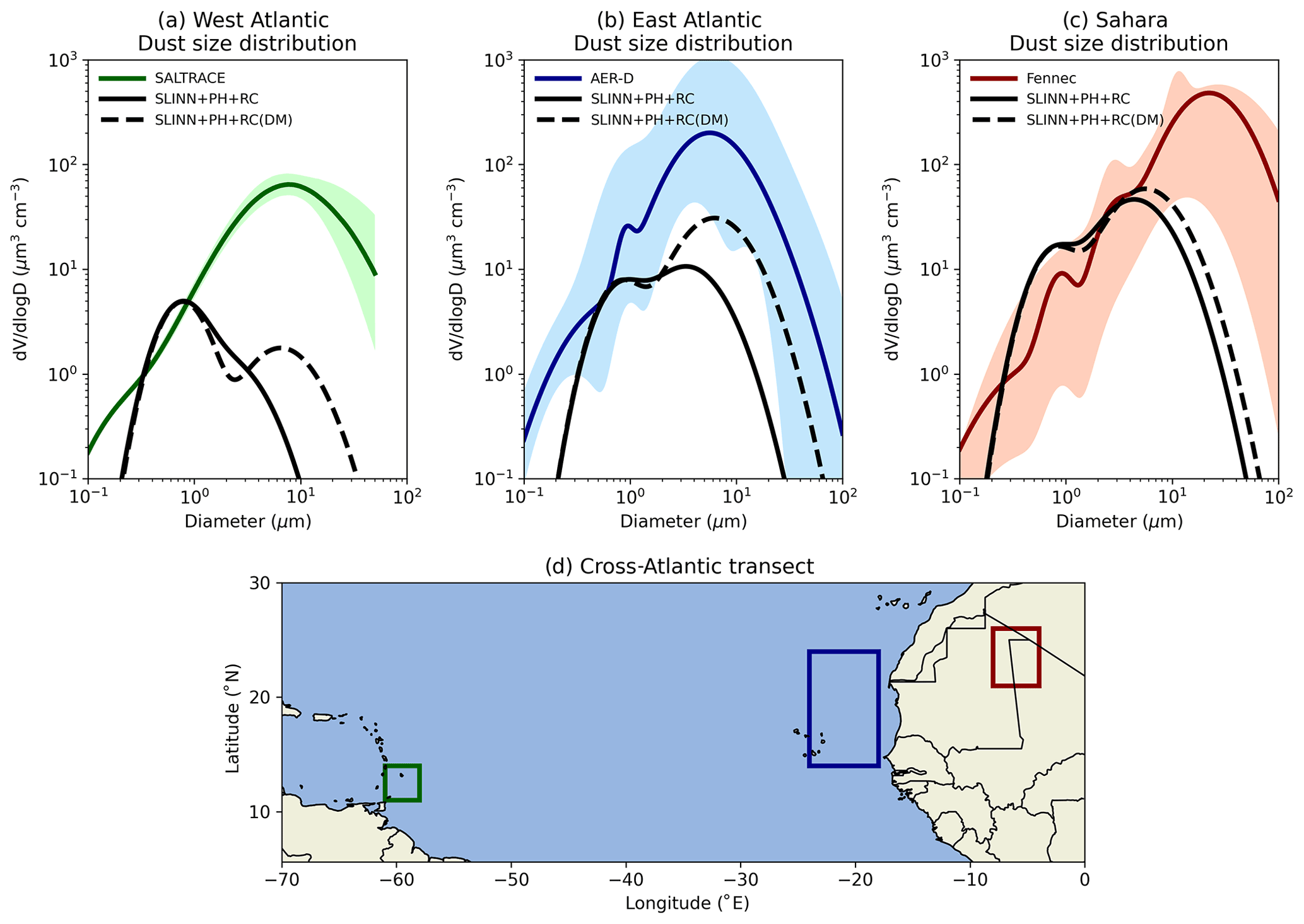
Figure 10 Dust volume size distributions in a cross-Atlantic transect in the SLINN+PH+RC and SLINN+PH+RC(DM) simulations for (a) June conditions in the region (58–61^∘ W, 11–14^∘ N) and 2–2.4 km altitude compared to SALTRACE measurements, (b) August conditions in the region (18–24^∘ W, 14–24^∘ N) and 2–3 km altitude compared to AER-D measurements, and (c) June conditions in the region (4–8^∘ W, 21–26^∘ N) and 0.1–1.2 km altitude compared to Fennec 2011 measurements. Panel (d) shows the horizontal boundaries of the averaging regions in the equatorial Atlantic.

Clearly mode merging has a sizeable impact on the distribution of dust mass between the two modes. Figure 9 shows the spatial dust metrics in the SLINN+PH+RC and SLINN+PH+RC(DM) simulations, and Fig. S11 shows the equivalent metrics for the LAAKSO and LAAKSO(DM) simulations. It is clear that downward mode merging has a negligible impact on the overall dust metrics; for instance, the spatial distribution and magnitude of the total dust burden are similar in SLINN+PH+RC (Fig.  S9a) and SLINN+PH+RC(DM) (Fig. S9c). The statistical measures of model fit compared to the observations, such as the biases and RMSEs, are equally comparable between the two simulations.

The main difference between the simulations becomes apparent when plotting the particle size distributions (PSDs). Figure 10 shows the volume size distributions (VSDs) for an equatorial cross-Atlantic transect, with simulated PSDs from SLINN+PH+RC and SLINN+PH+RC(DM) directly compared to observations from three independent summer (June–August) field campaigns. As a caveat, it is not possible to quantify how representative the observations are of the regional-mean dust PSDs, given that the aircraft campaigns measure a small sample space both spatially and temporally but often remain our only datasets to measure the vertical structure of regional atmospheric aerosol. Figure S12 shows the equivalent VSDs for LAAKSO and LAAKSO(DM), and Fig. S13 shows the number size distributions (NSDs) for all four simulations and observations.

It is clear from Fig. 10 that a significant amount of dust volume over the Saharan source region is missing in both SLINN+PH+RC and SLINN+PH+RC(DM) (Fig. 10c), which is at least partially caused by the inability of the current UKCA-mode scheme to represent super-coarse dust emissions. In order to rectify this, a third insoluble mode representing super-coarse dust aerosol may in future be added to UKCA-mode. Simulated VSDs for the accumulation and coarse modes (d_p<10 µm) are in good agreement with Fennec 2011 observations over the Sahara (Fig. S10c). Over the east Atlantic, the median diameter of the coarse mode is significantly greater in SLINN+PH+RC(DM) than in SLINN+PH+RC, which agrees better with the AER-D VSD observations (Fig. 10b), albeit with a large difference in absolute coarse-mode VSD, which is likely linked to the lack of super-coarse dust emissions (Fig. 10c). Finally, over the west Atlantic, the SALTRACE observations indicate a significant quantity of coarse-mode dust advected from the Sahara, which is not apparent in either simulation and may again be related to the inability to represent super-coarse dust emissions (Fig. 10a). Nevertheless, the median diameter of the coarse mode is in better agreement with SALTRACE in SLINN+PH+RC(DM) than in SLINN+PH+RC, and considerable coarse-mode mass is preserved in SLINN+PH+RC(DM) (Fig. 10a). In summary, Fig. 10 shows that downward mode merging acts to preserve coarse-mode mass during atmospheric transport and effectively counteracts the lack of contractibility of modes, which is an artefact of the double-moment modal architecture. Therefore, in answer to KQ4, it may be important to represent downward mode merging in modal aerosol schemes that resolve particle growth and contraction processes such as BCS, in order to correctly resolve the aerosol PSDs.

6 Conclusions and discussion

In this paper, various widely used parameterisations of the below-cloud scavenging (BCS) of aerosol by raindrops are presented and directly compared in climate simulations with the Met Office's Unified Model (UM-GA8.0). In particular, a new parameterisation is presented for the collection efficiency of particles due to rear capture in the wake of falling raindrops, which can be added to the established collection efficiencies due to Brownian motion, inertial impaction, interception, thermophoresis, diffusiophoresis, and electric charge effects (Wang et al., 2010). It is found that rear capture is the dominant BCS loss process for accumulation-sized particles under moderate to heavy rainfall conditions but has less of a cumulative impact on simulated dust concentrations in UM-GA8.0 than the addition of the three phoretic processes alone.

Four outstanding key questions (KQs) pertinent to numerical BCS schemes are answered in this paper, namely, as follows: what is the impact of using empirical rather than theoretical BCS schemes? (KQ1) How important are missing processes to the ubiquitous Slinn (1984) BCS scheme? (KQ2) What is the impact of using a single-moment rather than double-moment BCS approach? (KQ3) How important is it to represent mode merging alongside BCS in modal aerosol models? (KQ4). Note that while mode merging is investigated here in the context of BCS, it may be equally applicable to other atmospheric aerosol loss processes. To answer these KQs, 20-year simulations using UM-GA8.0 were performed, where the only variable is the underlying BCS scheme applied to UKCA-mode mineral dust aerosol. BCS rates were calculated offline and tabulated for simple interpolation as a function of aerosol median diameter, modal width, and ambient rain rate online in UKCA-mode. UKCA-mode mineral dust aerosol was selected because of its high potential for improvement, given that simulated dust concentrations are persistently too high in the default UKCA-mode dust setup, which has often been attributed to inefficient wet deposition processes. It is therefore an ideal aerosol candidate for this type of sensitivity study.

Our simulations have highlighted the high sensitivity of simulated dust aerosol to the choice of BCS scheme; for example, accumulation-mode dust lifetime ranged from 5.4 d (LAAKSO) to 43.8 d (SLINN) and coarse-mode dust lifetime ranged from 0.9 d (LAAKSO(DM)) to 4 d (SLINN+PH+RC(1M)). In answer to KQ1, the use of empirically derived BCS rates significantly underestimates dust concentrations and deposition rates away from source regions compared to observations (LAAKSO), whilst the theoretical BCS model exhibited dust concentrations comparable with observations (SLINN+PH+RC) (Fig. 7). This tentatively corroborates the suggestion by Wang et al. (2010, 2014) that the best BCS model to use in GCMs is the theoretical model with the greatest BCS rates (i.e. Slinn+ph+rc). Interestingly, the semi-empirical model by Wang et al. (2014) exhibits dust concentrations that are too high away from source regions in these simulations (e.g. over the Pacific, Pac; Fig. 7h). The statistical measures of fit (in particular, the bias and RMSE) used to compare simulated and observed DOD, surface dust concentrations, and deposition rates suggest that the WANG simulation may be closer to observations than LAAKSO or SLINN+PH+RC overall, but this appears to be a result of compensating errors, i.e. too little dust near source regions (e.g. west Atlantic, WAtl; Fig. 7h) and too much dust away from source regions (Pac; Fig. 7h). Given that the Wang scheme was fit to theoretical BCS models before the parameterisation of the rear-capture effect existed, and given that Wang et al. (2014) implicitly used many of the Slinn+ph parameterisations in their formulation of the Wang model, the use of the more physical Slinn+ph+rc BCS scheme in aerosol models appears to be the most accurate approach of those tested here.

In answer to KQ2, the addition of phoresis to the Slinn (1984) BCS model has a significant impact on simulated accumulation-mode dust burden akin to a halving globally (SLINN+PH vs. SLINN; Table 2 and Fig. 8). The addition of rear capture on top of phoresis to SLINN has a more muted impact than phoresis alone, which may be underestimated here given the inability of coarse-resolution GCMs to resolve heavy precipitation episodes and the non-linear increase in rear-capture collection efficiency with rain rate (Fig. 3). The relatively muted effect of the rear-capture mechanism (with regard to the modelled dust metrics) may also be consistent with the relatively narrow range in the raindrop sizes when the mechanism is important, as shown in Fig. 2, as well as possible buffering effects of the multiple processes in the model influencing the overall simulation results. Additionally, we have only tested the impacts of representing rear capture alongside phoresis (SLINN+PH) and not on its own (i.e. SLINN+RC), which is not a clean test for the importance of the rear-capture effect. In summary, neglecting the processes of rear capture and phoresis in the Slinn model may significantly overestimate submicron-sized (i.e. accumulation-mode) dust burdens.

KQ3 and KQ4 are particularly pertinent to modal aerosol schemes, which are widely employed by GCMs (Gliß et al., 2021). In answer to KQ3, the use of a single-moment BCS approach (applied to a double-moment aerosol scheme) which does not account for modal width has a small impact on the narrow accumulation mode but a large impact on the broad coarse mode. For example, the global coarse dust burden increases from 5.3 Tg in SLINN+PH+RC to 13.2 Tg in SLINN+PH+RC(1M) (Table 1). Therefore, a single-moment BCS scheme (as employed by default in UKCA-mode) may significantly underestimate the wet deposition of coarse-mode aerosol. In answer to KQ4, downward mode merging has little overall impact on total dust concentrations in this model (SLINN+PH+RC(DM) vs. SLINN+PH+RC; Fig. 9) but does have a significant impact on the partitioning of dust between the accumulation and coarse insoluble modes (Fig. 10). Given the structural limitation in the double-moment modal aerosol approach, i.e. the fixed mode width, downward mode merging may be a useful method to reconcile simulated and observed aerosol size distributions.

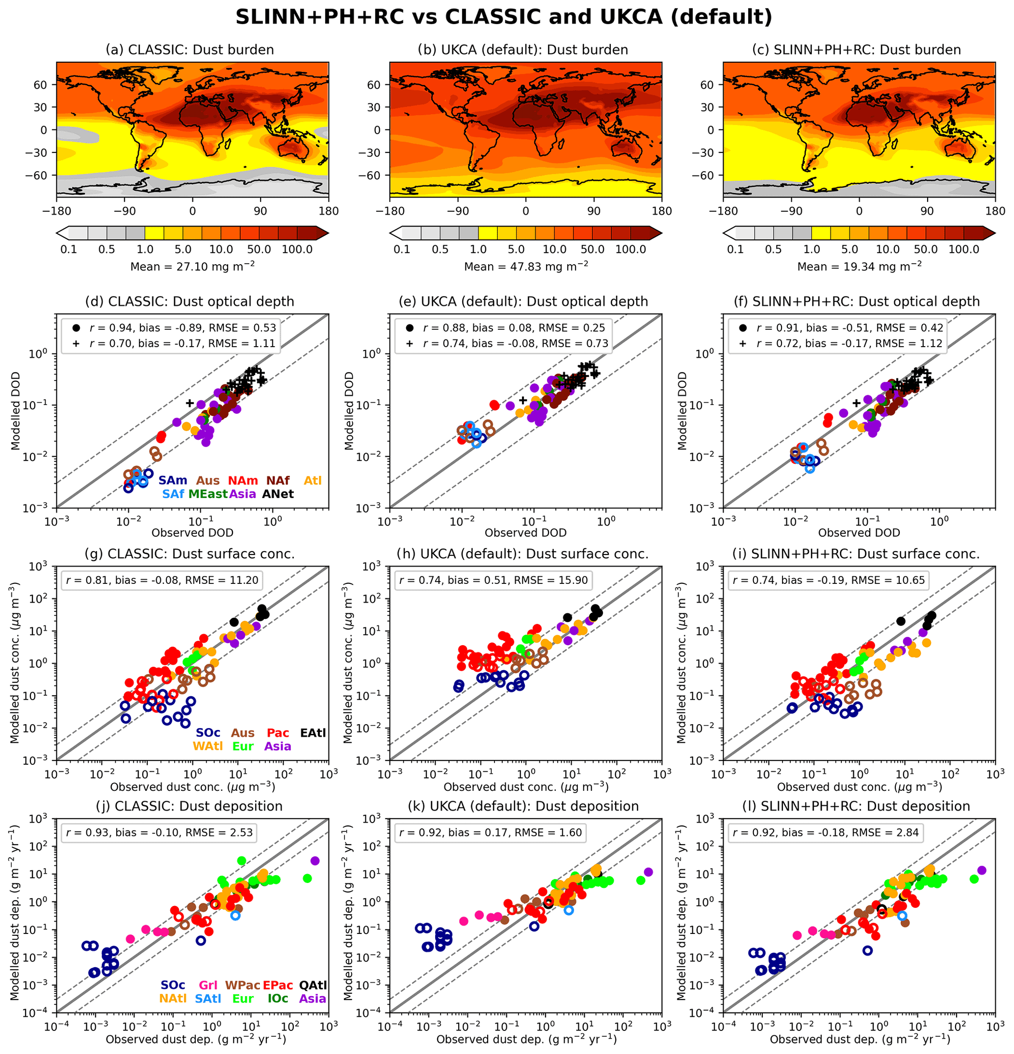
Figure 11 The same as Fig. 7 but used to compare the SLINN+PH+RC simulation with UM-GA8.0 with CLASSIC dust (left column) and UM-GA8.0 with UKCA-mode dust and its default BCS scheme. This is used to answer the supplementary question, the impact of the Slinn+ph+rc BCS scheme versus existing UM-GA8.0 schemes.

Although the primary aim of this study is to impartially compare various BCS schemes from the literature in an appropriate GCM framework with all else being equal, the stimulation for such a study was the inadequate performance of the existing UKCA-mode dust scheme compared to observations and to the default UM-GA8.0 dust scheme (CLASSIC). For full descriptions of the existing UKCA-mode and CLASSIC BCS schemes, see Mann et al. (2010) and Woodward et al. (2001), respectively. An interesting supplementary question (SQ) is then the following: how do the global dust metrics compare between a simulation with the new double-moment BCS setup (using the Slinn+ph+rc BCS model) and simulations with CLASSIC and with the default UKCA-mode dust scheme? To provide a preliminary answer to this question, which will be answered in more detail in a follow-on paper, the same configuration of UM-GA8.0 was employed as in the rest of this study for one simulation with CLASSIC dust in its default setup (six bins) (Woodward et al., 2022) and one for UKCA-mode dust with its existing single-moment BCS scheme (Mann et al., 2010). Global dust metrics in the SLINN+PH+RC simulation are compared to CLASSIC and default UKCA in Fig. 11. Although it is unclear whether the single-moment BCS approach is culpable for the inferior performance in UKCA (default) away from dust source regions (e.g. over the Pacific Ocean, Pac; Fig. 11h), given the many facets of the dust scheme, it is clear that simulated dust surface concentrations are markedly closer to observations away from source regions in SLINN+PH+RC than in UKCA (default) and are now comparable with CLASSIC dust. Although our tests have focused on AMIP simulations in a climate configuration, the efficiency of the new Slinn+ph+rc BCS scheme and the improved dust performance (Fig. 11) now makes UKCA-mode dust a candidate for global NWP simulations with the UM (e.g. Mulcahy et al., 2014).

This work has focused on BCS models for aerosol schemes. While we have shown that including a more theoretically based BCS model significantly improves the simulation of dust (e.g. comparing SLINN+PH+RC with LAAKSO; Fig. 7), we are not arguing that this is a panacea for dust modelling. For example, the work presented here uses just two modes to represent atmospheric dust, and this is not sufficient to resolve the observed size distribution near source regions, which leads to significant underestimation of volume associated with missing super-coarse particles and number associated with small Aitken particles (e.g. Fig. 10). This may be partially rectified in future by the addition of a third insoluble mode to represent super-coarse dust. Secondly, the ageing of dust from interaction with soluble atmospheric aerosols is not represented in the simulations, and therefore dust is not able to act as liquid CCN here (i.e. in-cloud scavenging), which is potentially an important atmospheric sink for mineral dust (Rodríguez et al., 2021). Even in its purely insoluble state, dust may act as CCN according to Köhler theory, which is not accounted for in these simulations. Therefore, the sensitivity of dust deposition to the choice of BCS scheme may be overestimated in these simulations given that ICS processes are not accounted for. In this work, the ageing scheme is not switched on but in the future work will be undertaken to assess the role of ageing in UKCA-mode dust simulations. Despite their limitations, UM-GA8.0 and UKCA-mode remain state-of-the-art climate and chemistry–aerosol models respectively (Sellar et al., 2020) and are ideally placed as a framework to perform such as an investigation as documented here.

The BCS scheme developed here has only been tested with one aerosol type (mineral dust), and in future it would be informative to test the scheme with other aerosols (e.g. sulfate, black carbon, organic carbon, and sea salt). In particular, soluble aerosol may be less sensitive to the underlying BCS model given its ability to act as CCN and therefore be efficiently removed from the atmosphere via ICS (Haywood and Boucher, 2000). The results also may differ if a model with a higher spatio-temporal resolution is employed given the non-linear propensity of aerosol “rear capture” to rain rate (Fig. 3) and the ability of a high-resolution model to resolve heavy precipitation episodes. Additionally, the BCS models described in Sect. 2 were processed offline assuming standard atmospheric conditions and making assumptions on, for example, the relationship between cloud droplet number density and rainfall rate, with the results tabulated and then used for simple interpolation in UKCA-mode. This is a computationally efficient method of evaluating BCS but does not account for differences in temperature, pressure, humidity, raindrop electric charge, or other atmospheric variables, which all affect BCS rates. Jung et al. (2003), Berthet et al. (2010), and Croft et al. (2010) offer numerical methods to explicitly evaluate BCS rates online, which may be a more refined and exact if computationally expensive approach.

The BCS scheme shown here employs a single parameterisation for the raindrop number density as a function of the rainfall rate from Abel and Boutle (2012) and a single parameterisation for the terminal velocity of falling droplets from Beard (1976). Wang et al. (2010) found that the choice of terminal velocity parameterisation could change BCS rates by a factor of 2, and the choice of raindrop number density could change BCS rates by a factor of 3–5. Therefore, the results presented here may be sensitive to the underlying parameterisations used for the raindrop properties. Finally, we have explored BCS for aerosol capture by liquid raindrops, but the current BCS scheme in UKCA-mode for aerosol capture by snow crystals is also a simple single-moment approach (Mann et al., 2010). Given the large differences between dust in the single- and double-moment BCS schemes (e.g. Fig. 9), it will be instructive to also improve the BCS scheme for snow, which may have a substantial impact on dust concentrations at high latitudes and in mountainous regions.

This study provides a summary of numerical modelling approaches for the below-cloud scavenging of aerosol by liquid raindrops and answers key questions concerning the implications of selecting one BCS scheme over another. It is found that the simulated accumulation-mode dust lifetime ranges from 5.4 d using an empirical BCS scheme (LAAKSO) to 43.8 d using a theoretical scheme (SLINN), while the coarse-mode dust lifetime ranges from 0.9 d (LAAKSO(DM)) to 4 d (SLINN+PH+RC(1M)), which highlights the high sensitivity of dust concentrations to the BCS scheme. Given the wide range of BCS rates from the different empirical and theoretical models, it would be useful to the aerosol modelling community to further constrain the range of BCS rates using laboratory experiments and to determine whether the disparity between the observed and theoretical BCS rates is truly due to confounding atmospheric processes.