the Creative Commons Attribution 4.0 License.
the Creative Commons Attribution 4.0 License.
 | 02 Sep 2022
Using aircraft measurements to characterize subgrid-scale variability of aerosol properties near the Atmospheric Radiation Measurement Southern Great Plains site
Jerome D. Fast
David M. Bell
Gourihar Kulkarni
Jiumeng Liu
Georges Saliba
John E. Shilling
Kaitlyn Suski
Jason Tomlinson
Jian Wang
Rahul Zaveri
Alla Zelenyuk
Complex distributions of aerosol properties evolve in space and time as a function of emissions, new particle formation, coagulation, condensational growth, chemical transformation, phase changes, turbulent mixing and transport, removal processes, and ambient meteorological conditions. The ability of chemical transport models to represent the multi-scale processes affecting the life cycle of aerosols depends on their spatial resolution since aerosol properties are assumed to be constant within a grid cell. Subgrid-scale-dependent processes that affect aerosol populations could have a significant impact on the formation of particles, their growth to cloud condensation nuclei (CCN) sizes, aerosol–cloud interactions, dry deposition and rainout and hence their burdens, lifetimes, and radiative forcing. To address this issue, we characterize subgrid-scale variability in terms of measured aerosol number, size, composition, hygroscopicity, and CCN concentrations made by repeated aircraft flight paths over the Atmospheric Radiation Measurement (ARM) program's Southern Great Plains (SGP) site during the Holistic Interactions of Shallow Clouds, Aerosols and Land Ecosystem (HI-SCALE) campaign. Subgrid variability is quantified in terms of both normalized frequency distributions and percentage difference percentiles using grid spacings of 3, 9, 27, and 81 km that represent those typically used by cloud-system-resolving models as well as the current and next-generation climate models. Even though the SGP site is a rural location, surprisingly large horizontal gradients in aerosol properties were frequently observed. For example, 90 % of the 3, 9, and 27 km cell mean organic matter concentrations differed from the 81 km cell around the SGP site by as much as ∼ 46 %, large spatial variability in aerosol number concentrations and size distributions were found during new particle formation events, and consequently 90 % of the 3, 9, and 27 km cell mean CCN number concentrations differed from the 81 km cell mean by as much as ∼ 38 %. The spatial variability varied seasonally for some aerosol properties, with some having larger spatial variability during the spring and others having larger variability during the late summer. While measurements at a single surface site cannot reflect the surrounding variability of aerosol properties at a given time, aircraft measurements that are averaged within an 81 km cell were found to be similar to many, but not all, aerosol properties measured at the ground SGP site. This analysis suggests that it is reasonable to directly compare most ground SGP site aerosol measurements with coarse global climate model predictions. In addition, the variability quantified by the aircraft can be used as an uncertainty range when comparing the surface point measurements with model predictions that use coarse grid spacings.
- Article
(5669 KB) - Full-text XML
-
Supplement
(3542 KB) - BibTeX
- EndNote


Complex distributions of aerosols evolve in space and time as a function of emissions, turbulent mixing and transport, coagulation, chemical transformation, phase changes, ambient temperature and humidity, cloud properties, and removal processes. These processes affect the number concentration, size distribution, chemical composition, mixing state, and microphysical properties of aerosols that ultimately determine the ability of aerosols to alter the radiation budget (e.g., Kaufman et al., 2002) and act as cloud- or ice-nucleating particles (Petters and Kreidenweis, 2007; DeMott et al., 2010). As aerosols are entrained into clouds, complicated aerosol–cloud interactions perturb cloud hydrometeors, albedo, growth, dissipation, lifetime, and precipitation, which influence climate (Twomey, 1974; Albrecht, 1989; Rosenfeld et al., 2014). The ability of models to represent the multi-scale processes affecting the aerosol life cycle depends not only on their ability to capture the important chemical and microphysical process, but also on their spatial resolution. Models often assume aerosol properties and meteorological conditions that influence aerosol evolution to be constant within a grid cell. As a result, coarse grid spacings currently used by Earth system models are not likely to resolve the large spatial variability of aerosol properties that are observed in many regions of the world (e.g., Anderson et al., 2003). While decades of work have gone into developing subgrid treatments of clouds in models (e.g., Arakawa and Schubert, 1974), characterizing and treating subgrid variability of aerosol processes have received far less attention. Subgrid-scale processes that affect aerosol populations could have a significant impact on the formation of particles, their growth to cloud condensation nuclei (CCN) sizes, aerosol–cloud interactions, dry deposition, wet scavenging, and hence their burden, lifetimes, and radiative forcing (e.g., Wang, 2007).
Modeling studies have explored subgrid-scale variability of aerosol properties and their effects on atmospheric forcing via their interactions with radiation and clouds by comparing the model predictions using different grid spacings. For example, climate model simulations in Ekman and Rodhe (2003) quantified the impact of anthropogenic sulfate on cloud albedo using grid spacings of 2.0 and 0.4∘. They found that the global mean indirect radiative forcing differed by only 7 %, and there was no difference in the temperature response. However, they did note larger regional differences in aerosol radiative forcing and atmospheric response. Qian et al. (2011) and Gustafson et al. (2011) used the chemistry version of the Weather Research and Forecasting model (WRF-Chem) with 75, 15, and 3 km grid spacings to determine differences in representing aerosol variability over Mexico and found that neglecting small-scale variations in aerosols led to biases in shortwave radiative forcing as large as 30 %. Wainwright et al. (2012) performed simulations using the chemistry version of the Goddard Earth Observing System model (GEOS-Chem) with grid spacings of 4, 2, and 0.5∘ and found that predicted secondary organic aerosol (SOA) concentrations depended significantly on model resolution because of nonlinear effects associated with SOA partitioning, lifetime, and precursor emissions. By using both a global climate model and WRF-Chem, Ma et al. (2014) showed that grid spacings much smaller than typical global climate models were needed to reproduce the observed black carbon plumes transported over the Pacific Ocean. Weigum et al. (2016) performed identical simulations using WRF-Chem except with grid spacings of 80 and 10 km and found that the coarser simulation of aerosol optical depth (AOD) was underpredicted by 13 % and that CCN concentration was overpredicted by 27 %.
These studies show that models are useful tools for investigating variability in aerosol properties and aerosol–radiation–cloud interactions associated with a range of grid spacings; nevertheless, measurements are critical for quantifying those variabilities observed in the atmosphere. While there are surface monitoring networks in North America, Europe, and parts of Asia that collect PM2.5 and PM10 measurements, the density of stations is often insufficient to fully characterize spatial variabilities in aerosol mass. In urban areas, emissions of aerosols and their precursors vary significantly, so that many monitors are needed to characterize variability in aerosol mass and a single monitor is not likely to be representative of a large area (e.g., Schutgens et al., 2017). The spatial representativeness of aerosol measurements is likely larger over rural areas, but the density of monitors also decreases. The distance between monitors varies between tens of kilometers to a few hundred kilometers apart, so that regional variability in aerosol mass may be underestimated in rural regions as well. Asher et al. (2022) recently described the spatial variability in aerosol number concentrations across a rural region around the Atmospheric Radiation Measurement (ARM) program's Southern Great Plains (SGP) site in northern Oklahoma using measurements from a network of seven Portable Optical Particle Spectrometers (POPS). They found that over a 5-month period concentrations of aerosols between 140 and 2500 nm in diameter varied by 10 %–20 % among the sites.
Satellite measurements have more complete spatial coverage than operational monitoring networks during clear-sky conditions, but they provide column-integrated quantities (e.g., AOD) and do not quantify more complex aerosol properties such as number, composition, and size distribution as a function of altitude. Therefore, aircraft platforms that deploy instrumentation capable of characterizing a wide range of aerosol properties have been used to fill in this data gap. Many research aircraft missions have been conducted over the past several decades to quantify variations in aerosol properties in many regions throughout the world. For example, Weigum et al. (2012) used the global HIAPER Pole-to-Pole Observations (HIPPO) over the Pacific Ocean and suggested that the horizontal variations in black carbon plumes could not be resolved by climate models at that time. Many aircraft field campaigns are designed to be surveys over global (e.g., Wofsy et al., 2011; Brock et al., 2019) to regional (e.g., Toon et al., 2016) scales. For these surveys, a specific region is sampled once that provides a “snapshot” of the variability that may or may not be representative of that region over a long period. Fewer aircraft campaigns have been conducted with repeated flight transects over a region. Those campaigns are often conducted over urban areas such as Houston (e.g., Parrish et al., 2009) and Los Angeles (Ryerson et al., 2013) to better understand aerosol formation and removal mechanisms rather than being used to characterize the spatial variability of aerosol properties.
In contrast to Asher et al. (2022), who quantified the spatial variability of aerosol number concentrations and size distributions using surface measurements, we address this issue by characterizing the subgrid-scale variability in terms of measured aerosol number, size, composition, hygroscopicity, and CCN concentrations using aircraft measurements from the Holistic Interactions of Shallow Clouds, Aerosols and Land Ecosystem (HI-SCALE) campaign (Fast et al., 2019) near the ARM SGP site. Repeated flights were conducted over a predominantly rural area ∼ 160 km wide in northern–central Oklahoma during the spring and late summer of 2016. Subgrid variability of aerosol properties is quantified for multiple grid spacings, ranging from those typically used by current cloud-system-resolving models as well as current and next-generation climate models. As will be shown later, surprisingly large horizontal gradients in aerosol properties were frequently observed even though the SGP site is a rural location. As expected, the smaller grid spacings capture more of the overall variability in aerosol properties; however, there is still substantial subgrid-scale variability using grid spacings of 3 km. We also find a seasonal dependence on subgrid-scale variability for some aerosol properties, with more variability during the spring for some properties and more variability during late summer for other properties. These seasonal differences are due, in part, to changes in variable precursor emissions of SOA and SOA formation rates. We also compare the aircraft measurements in the boundary layer with those collected at a surface site to determine the representativeness of the surface measurements.
Measurements of aerosol number, size, and composition were collected by the Department of Energy (DOE)'s Gulfstream-1 (G-1, Schmid et al., 2014) aircraft over northern–central Oklahoma near the ARM SGP facility (Sisterson et al., 2016) during the HI-SCALE campaign (Fast et al., 2019). Two Intensive Observational Periods (IOPs) were conducted by the G-1 aircraft, one in the spring between 24 April and 21 May and the other in the late summer between 28 August and 24 September; 17 and 21 flights were conducted during IOPs 1 and 2, respectively. One flight was conducted per day, except on 5 days during IOP 2, which had two flights per day. All flight paths during IOP 2 are shown in Fig. 1, which were similar to those during IOP 1. G-1 was based out of Bartlesville, Oklahoma, east of the SGP site; 66 % and 59 % of the flight time during spring and summer, respectively, occurred within 100 km of the SGP site's Central Facility. Since the observed winds during the IOPs are frequently from the south to southeast, as shown by wind roses in Fig. S1 in the Supplement, measurements were collected along two transects upwind of the SGP site on several days.
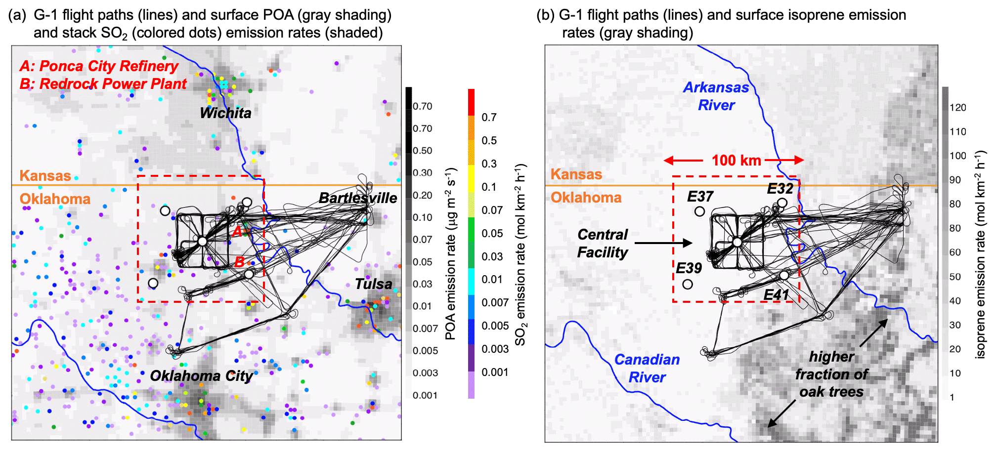
Figure 1G-1 flight paths near the ARM SGP site over northern–central Oklahoma during IOP 2 along with (a) surface POA (gray shading) and stack SO2 (colored dots) emissions and (b) surface isoprene emission rates (gray shading). Open circles denote primary SGP site vertical profiling measurement sites.
Table 1 lists the instrumentation and measurements of aerosol number, size, and composition used in this study to quantify the spatial variability of those quantities. Additional instrumentation deployed on G-1 and the resulting measurements are described in Fast et al. (2019). Two TSI Condensation Particle Counters (CPC models 3025 and 3010) were deployed to measure number concentrations for particle diameters greater than 3 and 10 nm. A coincidence correction (Aaron et al., 2013) has been applied to the CPC3010 to extend the detection limit from 10 000 to 80 000 cm−3 with an average discrepancy of less than 4 %. The Fast Integrated Mobility Spectrometer (FIMS, Wang et al., 2018) measured the number distribution for particle diameters between 9 and 426 nm. CCN number concentrations at two supersaturations (0.24 % and 0.46 %) were measured by a Droplet Measurement Technology (DMT) CCN counter. An Aerodyne Time-of-Flight Aerosol Mass Spectrometer (AMS, DeCarlo et al., 2006) provided bulk aerosol composition concentrations and mass concentrations for nonrefractory organic matter (OM), sulfate (SO4), nitrate (NO3), and ammonium (NH4) for particle diameters <1 µm in vacuum aerodynamic diameter particles. The average concentrations of OM, SO4, NO3, and NH4 for each flight are given in Tables S1 and S2. Detailed information on aerosol composition is provided by miniSPLAT (Zelenyuk et al., 2015), a single-particle mass spectrometer that characterizes the composition of individual particles with vacuum aerodynamic diameters between 50 nm and 2 µm. The observed aerosol mixing state during HI-SCALE is often complex (Fast et al., 2019), which is different than assumptions of internal or external mixtures of aerosol composition commonly used by climate models. To reduce the complexity of aerosol mixtures, particles sampled by miniSPLAT are divided into 11 classes as described in Table 2. Most of the classes have mixtures of different types of organics. miniSPLAT is also able to characterize refractory particles containing soot and dust that the AMS cannot detect. Two classes (Org_amins, Pyr) are not analyzed in this study since relatively few of those particles were observed during HI-SCALE. Particle classes were determined at 6 min intervals, which has implications for spatial variability that will be described later. The average particle class fractions for each flight are given in Tables S3 and S4.
Table 1Aerosol instrumentation deployed on the G-1 aircraft during HI-SCALE.

Given that the G-1 flight speed was 100 m s−1, each measurement at 1 s intervals from the CPC, FIMS, and CCN instruments represents average conditions over 100 m. In contrast, each measurement from the AMS and miniSPLAT average conditions was over 1.3 and 6 km, respectively.
At the Central Facility, similar instrumentation to that on the G-1 aircraft was deployed to obtain continuous measurements of aerosol number, size, composition, and CCN concentrations. We also use Doppler lidar measurements from the Central Facility, E32, E37, E39, and E41 sites denoted by the white circles in Fig. 1. The Doppler lidar provides vertical profiles of wind speeds and directions, but vertical gradients in the signal-to-noise (SNR) ratio are also used to determine the convective boundary-layer height as a function of time during the day. In this study, we use these heights to determine which aircraft flight legs are conducted within and above the boundary layer.
Emission rates of primary organic aerosol (POA) at the surface and sulfur dioxide (SO2) above the surface from the 2011 EPA National Emissions Inventory (NEI) are also shown in Fig. 1a to illustrate the spatial distribution of anthropogenic sources of aerosols and aerosol precursors in the region in relation to the G-1 flight paths. The Oklahoma City, Tulsa, and Wichita metropolitan areas have the largest urban emission rates in the region. There are also several large sources of SO2 located in rural areas, such as the Redrock Power Plant and the Ponca City Refinery near the SGP site. The G-1 aircraft frequently observed peak concentrations of SO2 and aerosol number close to these sources. As described in Liu et al. (2021), the AMS measurements indicated that organic matter made up the largest fraction of aerosol mass during both IOPs and that biogenic trace gas emissions likely contributed a significant fraction of the observed organic aerosol mass. As shown in Fig. 1b, the largest sources of isoprene emissions are located to the south and east of the SGP site, and southeasterly winds would transport fresh biogenic SOA towards the SGP site. These isoprene rates are based on the MEGAN model (Guenther et al., 2012), the spatial distribution coincides with the density of broadleaf trees (primarily oak) that emit isoprene, and the emission rates depend on meteorological conditions which are different between IOPs 1 and 2.
As described later, miniSPLAT measurements frequently detected particles with biomass burning markers during both IOPs. On a couple of days during IOP 1 (6 and 7 May, Table S3), biomass burning aerosols comprised a large fraction of the total aerosol number. Biomass burning emissions from the Fire INventory from NCAR (FINN, Wiedinmyer et al., 2011) in Fig. S2 indicate that the number of fires and emission rates was relatively low around the SGP site and that the number of fires was even lower during IOP 2. However, coupling air mass trajectories shown in Liu et al. (2021) with FINN suggests that fires as far north as North Dakota and southern Canada may have contributed to biomass burning aerosol during IOP 1. During IOP 2, biomass burning aerosols were likely transported by southeasterly winds from larger fires in Arkansas, Louisiana, and southeastern Texas. Taken together, Figs. 1, S1, and S2 suggest that local anthropogenic, biogenic, and biomass burning sources likely contributed to aerosols sampled by G-1 in addition to long-range transport.
Our objective is to compute the spatial variability of observed aerosol properties in relation to typical model grid cells that assume constant values within those grid cells. First, grid cells over the G-1 flight domain are defined with widths of 81, 27, 9, and 3 km as shown in Fig. 2. The 81 and 27 km cells represent typical grid spacings used in current climate models, while the 9 and 3 km cells represent typical grid spacings used by current weather forecast and chemical transport models. Next-generation climate models are expected to have similar spatial resolutions to current weather forecast models. Four 81 km cells encompass most of the HI-SCALE G-1 flight paths. This spatial configuration results in 36, 324, and 2196 cells for the 27, 9, and 3 km grid spacings, respectively. Mean values of aerosol number, aerosol composition, hygroscopicity, and CCN concentration are then computed for each cell, flight leg, and flight. Only data on constant flight legs are used, so that effects of vertical gradients on the subgrid-scale variability statistics are minimized. Data for flight legs within clouds (i.e., when cloud liquid water content exceeded 0.001 g m−3) are also excluded from the statistics.

Figure 2G-1 aircraft flight path on 7 May along with the (a) 81, (b) 27, (c) 9, and (d) 3 km boxes used to compute mean aerosol properties from the aircraft measurements.
For example, Fig. 3a shows the constant-altitude flight legs using alternating red and blue colors, and Fig. 3b shows the temporal variability of OM, SO4, NO3, and NH4 concentrations sampled by the AMS on 7 May. Horizontal gradients in OM over individual flight legs are evident by comparing Fig. 3a and b. In addition, the spatial variability of SO4, NO3, and NH4 over a particular flight leg can be quite different because of different aerosol precursor sources and secondary formation processes. The variability of the grid cell means for the 81 km cell centered over the SGP site (Fig. 3c) is shown in Fig. 3d. Mean OM concentrations for flight legs (green dots) within the 81 km cell are between 3.21 and 3.47 µg m−3. The range of the mean values increases for the 27 and 9 km cells; however, the range is similar for the 9 and 3 km cells. This suggests that a 9 km grid spacing captures much of the variability over the G-1 flight path. While the 3 km cells do not provide a larger range in cell means, they do result in a larger standard deviation of OM that reflects some small-scale variability that even the 3 km cell mean does not represent. Since the AMS sampling interval of ∼ 13 s results in only two to three samples within a single 3 km cell, we note that the AMS is already averaging out some of the variability that can be represented by instruments with 1 s sampling intervals.
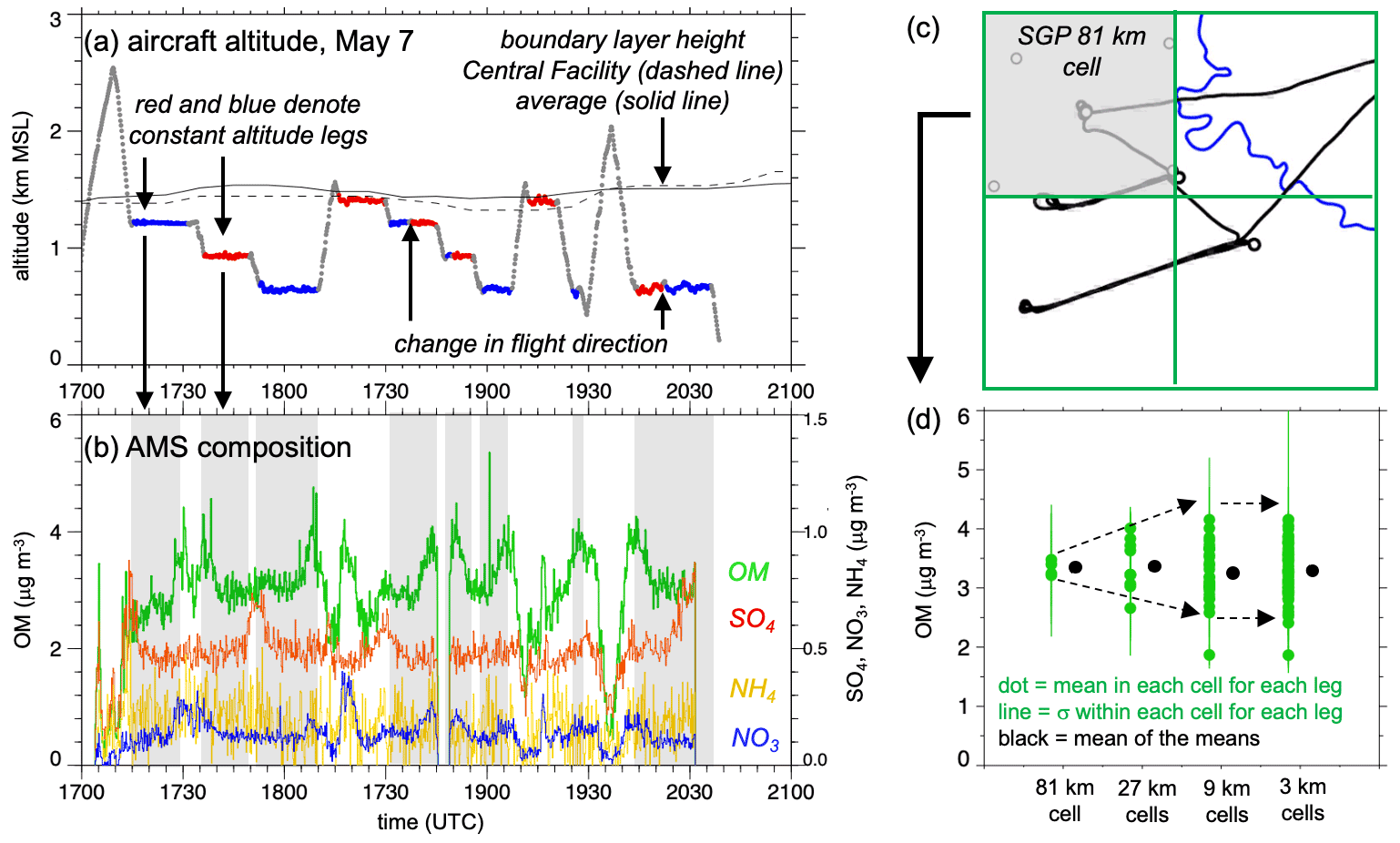
Figure 3G-1 aircraft (a) altitude on 7 May where the alternating blue and red colors denote different constant-altitude flight legs and (b) concentrations of OM, SO4, NO3, and NH4 measured by the AMS where gray shading denotes boundary-layer flight legs used to compute subgrid-scale variability. The gray shading in panel (c) denotes the 81 km cell around the SGP site associated with the 81, 27, 9, and 3 km cell averages and standard deviation of OM shown in panel (d).
It is possible that the different flight leg altitudes introduce vertical gradient variability into the horizontal gradient calculations. While it is reasonable to assume that vertical gradients of aerosols within the daytime convective boundary layer are likely to be small, there were large vertical gradients between the top of the boundary layer and the lower free troposphere. Therefore, flight legs are separated into those within and above the convective boundary layer using a combination of boundary-layer heights derived from the Doppler lidars (Tucker et al., 2009; Krishnamurthy et al., 2021) and visual inspection of vertical potential temperature gradients from aircraft and radiosonde measurements. Flight legs at the top of the boundary layer are excluded from those within the boundary layer. Since data from the Doppler lidars are not available prior to 3 May, boundary-layer depth is determined solely from radiosonde and aircraft measurements for the first five flights during IOP 1.
The average boundary-layer height determined from the five Doppler lidars is included in Fig. 3a to separate the flight legs into two groups. While there is some variability in the boundary-layer height across the SGP site, the average boundary-layer height among the five lidars is similar to the height at the Central Facility on 7 May. On this day, two constant-altitude flight legs are at or very close to the top of the convective boundary layer and are thus excluded from the analysis of spatial variability within the boundary layer. Relatively few flight legs were conducted in the lower free troposphere or near the boundary-layer top; therefore, we quantify subgrid-scale variability of aerosol properties only within the boundary layer.
We next compute a normalized frequency of the variable means over all flight legs by binning OM into concentration ranges of 0.5 µg m−3 and binning SO4, NO3, and NH4 into concentration ranges of 0.05 µg m−3 as shown in Fig. 4. Figure 4a shows the same information in Fig. 3d but in a slightly different manner. As in Fig. 3d, the mean OM concentrations over the 81 km cell fall within the 3.0–3.5 µg m−3 bin, and the mean cell concentrations for the 27, 9, and 3 km cells have a larger range between 2.5 and 4.5 µg m−3. Similarly, the smaller grid spacings resolve more of the spatial variability in SO4, NO3, and NH4 (Fig. 3b–d).
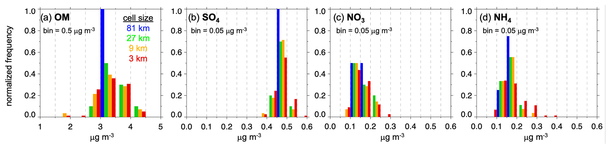
Figure 4Normalized frequency of occurrence for (a) OM, (b) SO4, (c) NO3, and (d) NH4 concentrations observed for the 7 May flight shown in Fig. 3b.
Similar statistics on the normalized frequency can be computed for all flights and for aerosol number, composition, hygroscopicity, and CCN concentration. For example, Fig. S3 depicts the normalized frequency of aerosol composition for all flights during IOP 1. However, this method will include day-to-day variations in the mean concentrations (Tables S1 and S2), which complicates the quantification of overall horizontal variability during the campaign. Instead, we compute percent differences from the 81 km cell mean given by Eq. (1) for each flight leg and variable within an IOP. Then, percentiles are used to express the departures from the 81 km cell mean. This removes the day-to-day variability as well as temporal variability within the same flight, so that all the flight statistics can be lumped together, which will be shown in the next section.
We note that there are two additional assumptions that will affect the computed spatial variability statistics. First, the aircraft flight path does not sample a large portion of a grid cell. At a minimum, it represents a transect across the grid cell; therefore, we assume that the spatial variability along that line is consistent with the variability within the entire cell. This is analogous to cloud chord sampling (e.g., Barron et al., 2020; Griewank et al., 2020). However, there were some flights that had a grid pattern near the Central Facility (Fig. 1) which would permit multiple transects across the 81 and 27 km grid cells. Second, temporal variability is not totally removed from these calculations. Individual flight legs were usually 10 to 20 min in duration. Aerosol number, size distribution, and composition, which influence CCN concentration, can be affected by secondary chemical formation processes over that period; however, we assume that those effects are smaller than the spatial variability present over a flight leg.
4.1 Bulk aerosol composition
Figure 5 shows the variability in aerosol composition for all flight legs during IOPs 1 and 2 relative to the coarse 81 km cell around the SGP site. For OM (Fig. 5a), 50 % of the 27, 9, and 3 km cell means are within 7 %–13 % of the coarse cell mean, while 90 % of the 27, 9, and 3 km cells are within 28 %–46 % of the coarse cell mean. The spatial variability of SO4 (Fig. 5b) is somewhat smaller than OM since 90 % of the 27, 9, and 3 km cells are within 23 %–35 % of the coarse cell mean. In contrast, 50 % of the 27, 9, and 3 km grid cell means for NO3 (Fig. 5c) during IOP 1 are within 16 %–33 % of the coarse cell mean, and 90 % of the grid cell means are within 52 %–64 % of the coarse cell mean, which is much larger than the spatial variability of OM and SO4. The spatial variability in NH4 (Fig. 5d) is somewhat greater than SO4 but less than NO3. The coarser 27 km cell means represent a large fraction of the spatial variability produced by the 9 and 3 km cell means when all the aircraft measurements are lumped together by the IOP. For all four composition species, the 3 km cells have a somewhat broader distribution as evident by a larger range between the minimum and maximum values and relatively fewer values closer to zero than the 27 km cells. In general, all the variability among all the 3 km cell means is within ∼ 100 % of the coarse grid cell mean.
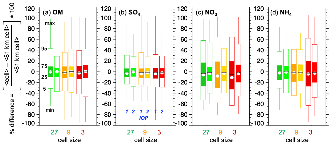
Figure 5Percent difference between the SGP 81 km cell average and the 27, 9, and 3 km cell averages of (a) OM, (b) SO4, (c) NO3, and (d) NH4 concentrations from the AMS instrument expressed as percentiles where the white circles denote the median values. All flights during IOPs 1 and 2 are grouped by the darker (left) and lighter (right) colors, respectively. Filled boxes denote values falling within the 25th to 75th percentiles, open boxes denote values falling within the 5th to 95th percentiles, vertical lines denote minimum and maximum values, and the black horizonal lines denote the mean values.
It is important to note that during IOP 2 the average OM concentrations were 1.3 µg m−3 (52 %) higher, SO4 concentrations were 0.5 µg m−3 (63 %) higher, NO3 concentrations were 0.16 µg m−3 (64 %) lower, and NH4 concentrations were 0.025 µg m−3 (6 %) higher than during IOP 1, as described by Liu et al. (2021) and reflected by the distribution of concentrations shown in Fig. S4. In addition to meteorological conditions being more conducive to SOA formation during IOP 2, local peak concentrations around the SGP site produce additional variability in OM, as reflected by the broader distribution of the absolute difference between the 3 km cell means within the coarse cell mean as shown in Fig. S5. Similarly, the absolute difference in NO3 has more local variability around the SGP site during IOP 1. Inspection of individual IOP 1 flights shows that there were short periods of relatively large NO3 concentrations, suggesting there were local NO3 hotspots as G-1 passed over the SGP site. The events that occurred were less frequent during IOP 2, most likely because temperatures were significantly higher during the late-summer period, which would affect the temperature dependence of NO3 on gas-to-particle partitioning processes. In contrast, the distributions of the absolute differences for SO4 and NH4 are similar for IOPs 1 and 2.
Since Eq. (1) normalizes the results by the 81 km cell mean, much of the seasonality of absolute spatial differences in OM is removed, as indicated by Fig. 5a. However, Fig. 5c shows that Eq. (1) still leads to smaller spatial variability of NO3 during IOP 2. For example, the 25th to 75th percentile range during IOP 2 is within 8 %–19 % of the coarse cell mean, which is smaller than the 16 %–33 % range during IOP 1.
Since total aerosol mass is dominated by organics, spatial variability in total mass concentrations over the SGP site will look similar to Fig. 5a in terms of percent differences of OM from the 81 km cell mean. In terms of absolute differences, the spatial variability of total mass concentrations over the SGP site is expected to be larger during the summer IOP, as with OM shown in Fig. S5. The variations among the 27, 9, and 3 km cells as well as the seasonality for all four 81 km cells shown in Fig. 2a are very similar to those in Fig. 5 (not shown).
4.2 Single-particle composition
The aerosol class information from miniSPLAT is expressed as a number fraction of the total number of characterized particles. To account for aerosol loadings, we compute subgrid variability for the aerosol classes (Table 2) in terms of aerosol volume by multiplying the particle fraction and the total volume measured by FIMS. This assumes the same FIMS-measured size distributions for all aerosol classes, while in reality, some particle classes are likely to be more frequent at small (i.e., soot) and large (i.e., dust) sizes. In addition, miniSPLAT provides critical information on aerosol composition during IOP 2 for the flights between 30 August and 7 September when the AMS was not functioning.
Table 2Particle classes defined from miniSPLAT single-particle measurements.
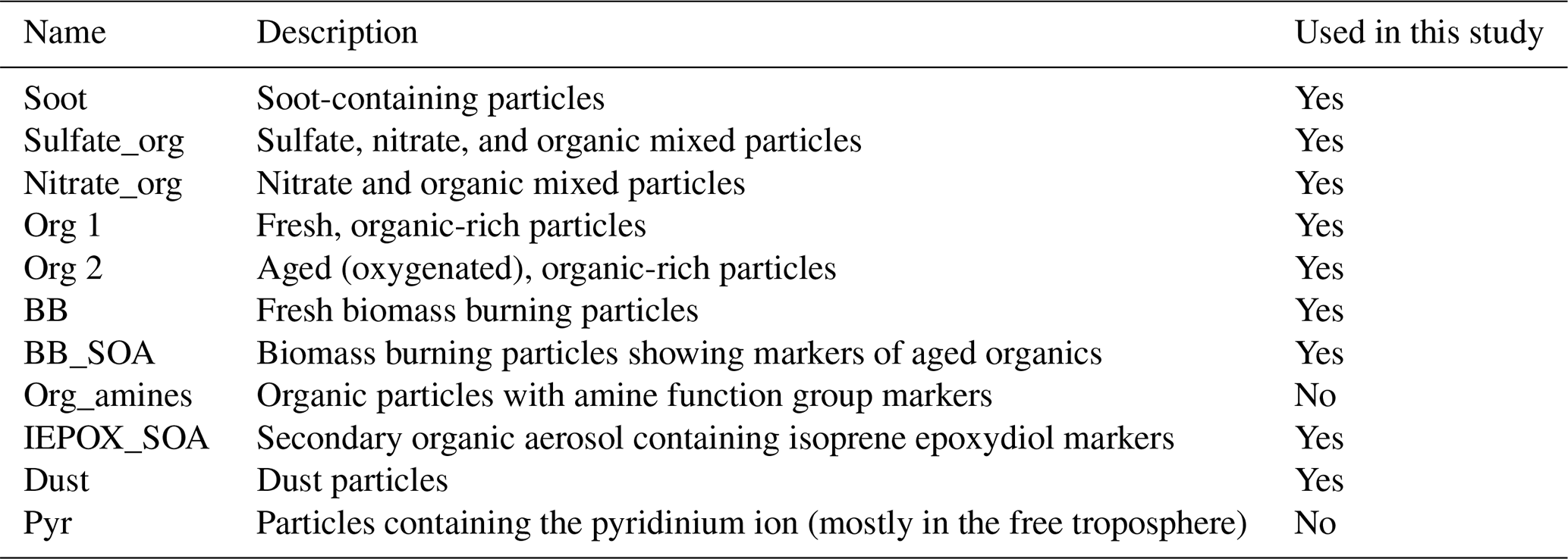
Figure 6 shows the spatial variability of nine particle classes from miniSPLAT for all aircraft flights during IOPs 1 and 2 in terms of percent difference from the 81 km cell mean. The percentiles for the Sulfate_org, Nitrate_org, IEPOX_SOA (for IOP 2), Org 1, Org 2 (for IOP 2), BB_SOA, and BB classes in Fig. 6 are similar to the statistics on bulk OM (Fig. 5) in terms of having a wider range between the 5th and 95th percentiles among the 3 km cells compared with the 27 km cells. However, the departures from the coarse cell mean for these five particle classes is larger than for bulk OM measured by the AMS. For example, 90 % of the 27, 9, and 3 km cells for OM are within 28 %–46 % of the coarse cell mean, while 90 % of these five particle classes are within 42 %–87 % of the coarse cell mean. In addition, the Org 1 (fresh organic-rich) and Org 2 (aged organic-rich) classes (Fig. 6d, e) have smaller departures from the coarse cell mean during IOP 2; 90 % of the 27, 9, and 3 km cells during IOP 1 are within 61 %–81 % of the coarse cell mean, which shrinks to 28 %–41 % during IOP 2. These differences are likely due to the relative contributions of organic-rich particles during the two IOPs, with significantly higher contributions from fresh and aged organic-rich particles during IOP 2 compared with IOP 1. Many days during IOP 1 were dominated by the sulfate-organic mixtures (Sulfate_Org) or biomass burning particles (BBOA_SOA and BB), with relatively small contributions of organic-rich particles and larger spatial variability over the SGP site. In contrast, the largest fractions of organic aerosols on most days during IOP 2 were comprised of organic-rich particle classes (Org 1, Org 2) that were more evenly distributed over the SGP site. The smaller fraction of the Sulfate_org particle class during IOP 2 is consistent with the lower SO4 concentrations observed by the AMS during IOP 2 compared with IOP 1.

Figure 6Percent difference between the SGP 81 km cell average and the 27, 9, and 3 km cell averages of (a) Sulfate_org, (b) Nitrate_Org, (c) IEPOX_SOA, (d) Org1, (e) Org2, (f) soot, (g) BB_SOA, (h) BB, and (i) dust volume concentration classes from the miniSPLAT instrument. The definition of percentiles and average values is the same as Fig. 5. All flights during IOPs 1 and 2 are grouped by the darker (left) and lighter (right) colors, respectively.
Another aspect of the distributions of the organic classes is that some classes during IOP 1, such as Nitrate_Org and Org 1, are more skewed than others. This has implications if models wish to represent subgrid-scale variability of aerosol properties in some way. This is analogous to how some cloud parameterizations (e.g., CLUBB, Golaz et al., 2002) use assumed Gaussian or double Gaussian probability density distributions to represent subgrid-scale variability of cloud properties.
While soot is usually a small fraction of total aerosol mass, it still has an important role in direct aerosol shortwave radiative forcing. Figure 6f shows that the 3 km cells have a larger range than the 27 km cells and 90 % of the 3 km cell means within 65 %–72 % of the coarse cell mean, reflecting contributions of both local and distant anthropogenic sources to spatial variability in this predominantly rural location. The observed distribution of soot is also skewed, and neglecting this skewness within coarse climate model grid cell averages may lead to uncertainties in the predictions of aerosol absorption. The spatial variability of fine-mode dust and its skewed distribution (Fig. 6i) is similar to that of soot, and coarse climate model grid cell averages may also lead to uncertainties in the aerosol longwave radiative forcing.
Since the particle class information from miniSPLAT was computed over 6 min intervals, which represents an average over 6 km, the 9 and 3 km cell percentiles in Fig. 6 are nearly the same. Therefore, the actual spatial variability in aerosol mixing state may be larger than suggested by the 9 and 3 km cells in Fig. 6.
For reference, Fig. S6 shows the absolute differences between the 3 km cell means and coarse cell means for the nine particle class volumes during IOPs 1 and 2. The single-particle measurements reveal that aerosol composition is far more complex than the bulk AMS composition measurements, and the spatial variability differs among the particle classes. These differences in the bulk and single-particle representations have implications for the overall hygroscopicity of particle populations and consequently concentrations of CCN and aerosol–cloud interactions.
4.3 Aerosol number concentration and size distribution
Figure 7 illustrates the temporal variability on the 7 May aircraft flight for the particle number concentration from the CPC3025 and FIMS instruments along with the CCN concentration at 0.24 % supersaturation. Large spatial gradients in aerosol number concentrations were observed along the individual flight legs, with peak concentrations frequently exceeding 6000 cm−3 (Fig. 7a). While CPC3025 measurements show that high aerosol number concentrations were observed at many locations around the Central Facility (Fig. 7b), continuous ground measurements of aerosol size distribution at the Central Facility (not shown) did not indicate a strong new particle formation event on this day. The spatiotemporal variations in number concentration from FIMS were similar to those from the CPC3025, although the concentrations were lower. Comparison of CPC3025 and FIMS concentrations shows that a large fraction of particles was smaller than 9 nm in diameter. Since the smallest particle diameters from the CPC3010 and FIMS instruments are nearly identical, the CPC3010 concentrations are close to those from FIMS and are therefore not shown for clarity. In addition, the FIMS number concentrations for diameters between 49 and 426 nm are shown to represent the variations in the lower portion of the accumulation-mode size range.
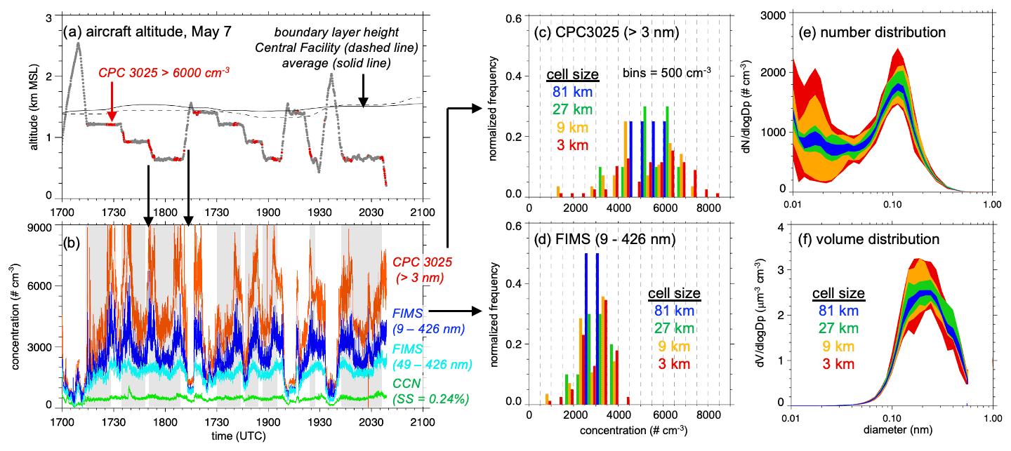
Figure 7G-1 aircraft (a) altitude on 7 May where the alternating red colors denote locations of peak number concentrations and (b) number concentrations from the CPC3025, FIMS, and CCN instruments where the gray shading denotes boundary-layer flight legs used to compute subgrid-scale variability. Normalized frequency from the (c) CPC3025 and (b) FIMS instruments and the (e) number and (f) volume distribution associated with the 81, 27, 9, and 3 km cell averages within the 81 km cell around the SGP site.
The normalized frequency of the mean number concentrations over 500 cm−3 bin intervals from CPC3025 and FIMS number concentrations are shown in Fig. 7c and d, respectively, for the 81, 27, 9, and 3 km cells. For the 81 km cell around the SGP site, mean CPC3025 concentrations (Fig. 7c) along the flight legs occurred within four bins between 4500 and 6500 cm−3. Progressively wider distributions are produced for the smaller grid cells, so that the peak mean concentrations increase to 6500–7000, 7000–7500, and 8500–9000 cm−3 for the 27, 98, and 3 km cell sizes, respectively. The results from FIMS (Fig. 7d) are similar to those from the CPC3025, except that the highest frequencies occur at lower concentrations. Figure 7c shows that the 3 km cells have the broadest distribution and thus capture more of the variability of small particles from the CPC3025, while both the 3 and 9 km cells captured much of the variability of the larger particles measured by FIMS, as shown in Fig. 7d. The range of the aerosol number and volume distribution within the 81 km cell around the SGP site is shown in Fig. 7e and f, respectively, to illustrate the differences among the 81, 27, 9, and 3 km cells as a function of aerosol diameter. The range of aerosol number (Fig. 7e) is largest for diameters less than 50 nm on this day, consistent with Fig. 7c. The spatial variations in the accumulation-mode aerosol volume (Fig. 7f) are similar to the variability of organic aerosol mass (Fig. 4a).
These results imply that coarse climate models are not likely to represent the variability of number concentrations over land, especially on days when new particle formation processes that produce high concentrations of ultrafine particles are important.
The spatial variability of number concentrations for all aircraft flights during IOPs 1 and 2 in terms of percent difference from the 81 km cell mean is shown in Fig. 8. For IOP 1, the ranges of the 5th and 95th percentiles for the 27, 9, and 3 km cells are very similar for the CPC3025 (Fig. 8a) and CPC3010 (Fig. 8b) measurements for diameters greater than 3 and 10 nm, respectively; 90 % of the grid cells means are within 36 %–55 % and 41 %–55 % of the coarse grid cell for particle diameters greater than 3 and 10 nm, respectively. Nevertheless, the range of the remaining 10 % becomes progressively larger for the 27, 9, and 3 km cells. In contrast, the ranges of values for the 27 km cells are larger than the 9 and 3 km cells for IOP 2, which is counterintuitive. The spatial variability is also much larger and more skewed during IOP 2, with 90 % of the grid cells means with 45 %–68 % and 47 %–64 % of the coarse grid cell for diameters greater than 3 and 10 nm, respectively. Fast et al. (2019) note that 20 and 6 new particle formation (NPF) events were observed during IOPs 1 and 2, respectively, but these results show that the overall spatial variability of number concentrations also differed between the IOPs. During IOP 1, high number concentrations were frequently observed over a large portion of the SGP site, similar to the distribution on 7 May (Fig. 7a, b). Except for a couple of flights, peak number concentrations were more often isolated and usually associated with emissions from the Redrock Power Plant and the Ponca City Refinery (Fig. 1a) during IOP 2. Therefore, the smaller spatial variability represented by the 27, 9, and 3 km cells during IOP 1 (Fig. 8a and b) reflects the more uniformly distributed number concentrations over the 81 km cell even though the number concentrations tend to be higher during IOP 1 than during IOP 2 (Fig. S7).
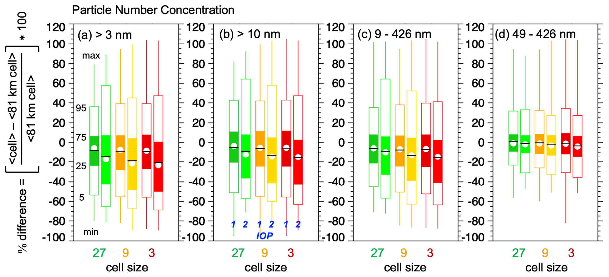
Figure 8Percent difference between the SGP 81 km cell average and the 27, 9, and 3 km cell averages of number concentrations with particle diameters (a) >3 nm (CPC3025), (b) >10 nm (CPC3010), (c) 9–426 nm (FIMS), and (d) 49–426 nm (FIMS). The definition of percentiles and average values is the same as Fig. 5. All flights during IOPs 1 and 2 are grouped by the darker (left) and lighter (right) colors, respectively.
Since the lowest size bin from FIMS is close to the smallest particle measured by the CPC3010, Fig. 8b and c are similar for the 27, 9, and 3 km cell as well as the differences between the IOPs. When the smallest particles less than 49 nm in diameter are removed, Fig. 8d shows that the spatial variability in number concentrations decreases significantly. For this size range, 90 % of the 27, 9, and 3 km cells are within 23 %–34 % and 27 %–35 % of the coarse cell mean for IOPs 1 and 2, respectively. This range is comparable with the range of OM mass concentrations where most of the mass is in the accumulation mode. For reference, the absolute differences in number concentrations during IOPs 1 and 2 between the 81 and 3 km cells are shown in Fig. S8, which shows that these differences are frequently as large as 4000 cm−3 when including ultrafine aerosol sizes and 500 cm−3 when considering accumulation-mode sizes.
It is important to note that the variability expressed in Fig. 8 is larger than the 10 %–20 % spatial variability in aerosol number concentrations over the SGP site reported by Asher et al. (2022). The differences between this study and Asher et al. (2022) are likely due to three factors. First, the POPS instrument measures particles as small as 140 nm, which neglects Aitken and ultrafine particles that are measured by the CPC and FIMS instruments. Second, the surface measurements in Asher at al. (2022) were collected during the fall and winter months between mid-October 2019 and mid-March 2020, and therefore the spatial variability may differ from aerosol populations observed during the spring and late summer as sampled during HI-SCALE. Finally, the different methodology of quantifying spatial variability from fixed surface sites and aircraft paths is likely a contributing factor.
The previous statistics on aerosol number hide important spatial variability in aerosol number and volume distributions that has implications for CCN, since it depends strongly on aerosol size (e.g., Dusek et al., 2006; Pöhlker et al., 2016; Patel and Jiang, 2021). The range of aerosol number and volume distribution in Fig. 7e and f suggests that the Aitken and accumulation modes each consist of a single mode diameter. Aerosol number and volume distribution averaged over an 81 km cell will likely have a simple, smooth distribution. New representations of aerosol formation and growth processes in climate models that better agree with such averaged observations may be obtaining the right answer for the wrong reasons because the spatial variability of aerosol and growth processes is likely to be far more complicated. For example, 81 km mean aerosol number and volume size distributions for 17 September and 7 May are shown in Fig. 9 along with select distributions from seven 3 km cells within the 81 km cell. On 17 September during a new particle formation event (Fig. 9a), the aerosol number concentration of the Aitken mode is about twice that of the accumulation mode. The average Aitken-mode diameter for the 81 km cell occurs at 30 nm, while the Aitken-mode diameters from select 3 km cells range between 20 and 40 nm, indicating variability in the growth rate of the Aitken mode over the 81 km cell. Interestingly, the aerosol volume size distributions from 3 km cells show a distinct bimodal distribution within the accumulation mode. While the bimodal distribution is still visible in the 81 km cell averaged accumulation volume mode, it appears to be less pronounced than the 3 km cell averages. Zaveri et al. (2022) found similar bimodality progressively developing within the accumulation volume mode in aged urban air in the Amazon. They used a detailed aerosol box model to interpret this behavior and attributed it to preferential growth of the smaller Aitken-mode particles from SOA formation at the expense of slow, bulk diffusion-limited growth of the preexisting semisolid accumulation mode. This aerosol growth behavior, however, could not be reproduced by the equilibrium SOA partitioning approach typically used in many chemistry–aerosol–climate models.

Figure 9Aerosol number and volume size distributions on (a) 17 September and (b) 7 May. Black line denotes the average within the 81 km cell over the SGP site, and the color lines denote select 3 km cell averages within the same 81 km cell.
On 7 May in Fig. 9b, the Aitken-mode number concentrations are about half that of the accumulation mode for the 81 km average. While the 3 km cells show that the number concentrations for particle sizes less than 40 nm can be up to a factor of 2 larger than the 81 km average, these variations are much smaller than those on 17 September. In addition, the overall shape of the aerosol number distributions from the 3 km cells tends to be similar to the 81 km average, in contrast to 17 September. Nevertheless, the aerosol volume size distributions from the 3 km cells still exhibit the characteristic bimodality within the accumulation mode, suggesting a history of rapid Aitken-mode growth and bulk diffusion-limited growth of the preexisting semisolid accumulation mode from SOA formation.
Overall, the results in Fig. 9 show important differences in aerosol number and volume size distributions over the 81 km cell region that reflect subgrid-scale variability in the new particle formation events and the subsequent particle growth rates due to variable precursor emissions and meteorological conditions. Thus, an equilibrium aerosol treatment used in a coarse climate model that may approximately reproduce the average aerosol number and volume size distributions, such as the 81 km cells shown in Fig. 9, may not work at progressively higher spatial resolutions, where more variability and important features are seen in aerosol size distributions due to variability in NPF rates and complex aerosol growth behaviors.
4.4 Cloud condensation nuclei and hygroscopicity
CCN are an important metric for climate models, since they drive aerosol–cloud interactions that influence the Earth's radiation budget and precipitation patterns. The representations of aerosol–cloud interactions in climate models remains highly uncertain (Boucher et al., 2013; Szopa et al., 2021) because of the non-coincident spatiotemporal variations in aerosol and cloud populations and their representation by coarse grid spacings as well as parameterized treatments of aerosol and cloud properties.
The spatial variability of CCN from the G-1 flight legs during IOPs 1 and 2 at two supersaturations is shown in Fig. 10a. For CCN at 0.24 % supersaturation during IOP 1, 50 % of the 27, 9, and 3 km cell means are within 4 %–8 % of the coarse cell mean and 90 % of the cell means are within 22 %–38 % of the coarse cell mean. The remaining 10 % of the 3 km cells differed by as much as 100 % of the coarse cell mean. During IOP 2, the spatial variability is somewhat larger for the 25th to 75th percentiles, which are within 6 %–11 % of the coarse cell mean. However, the maximum differences with the coarse cell mean are similar for the 27, 9, and 3 km cells. For CCN at 0.46 % supersaturation, 50 % of the 27, 9, and 3 km cell means are within 5 %–15 % of the coarse cell mean, which is somewhat larger than for CCN at 0.24 % supersaturation. While the percent differences among the 27, 9, and 3 km cells and between the IOPs differ somewhat, the spatial variability for CCN at both supersaturations is similar, with little skewness and medians close to zero. Interestingly, the 5th to 95th variability in CCN concentrations among 27, 9, and 3 km is significantly lower than the observed variability in aerosol composition and mixing state (Fig. 6) and number concentrations (Fig. 8), especially at the 0.24 % supersaturation, even though both aerosol properties determine their CCN activity. This result indicates that improved representations of aerosol formation and growth processes may result in modest improvements in CCN concentrations and variability at ambient supersaturation levels and hence modest changes in modeled indirect radiative effects.
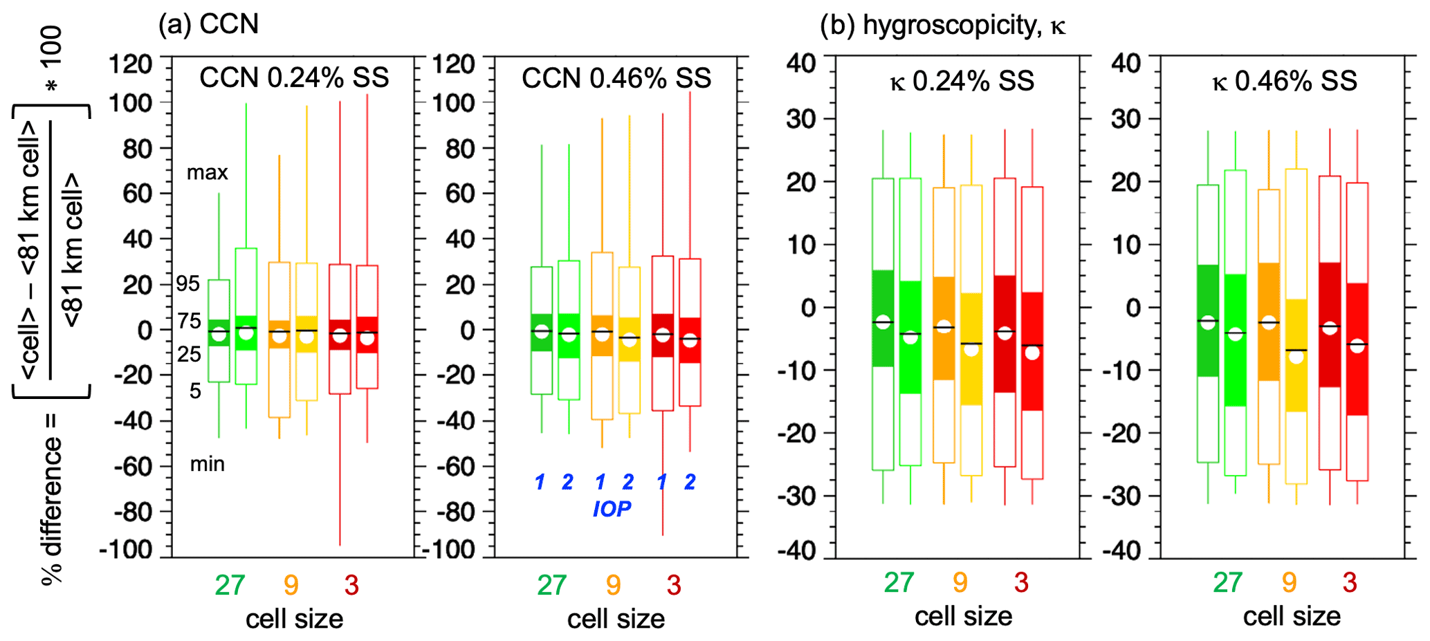
Figure 10Percent difference between the SGP 81 km cell average and the 27, 9, and 3 km cell averages of (a) CCN and (b) hygroscopicity, κ, at 0.24 % and 0.46 % supersaturation. The definition of percentiles and average values is the same as Fig. 5. All flights during IOPs 1 and 2 are grouped by the darker (left) and lighter (right) colors, respectively.
CCN concentrations at 0.46 % supersaturation are usually higher than those at 0.24 %, and CCN at both supersaturations is usually higher during IOP 2 (Tables S1 and S2), when number concentrations were also higher. The higher CCN concentrations during IOP 2 drive more spatial variability in absolute differences between the 81 and 3 km cells, as shown in Fig. S9a. For CCN at 0.24 % supersaturation, most of the 3 km cells are within 100 and 200 cm−3 of the 81 km cell for IOPs 1 and 2, respectively. Most of the 3 km cells are within 200 and 300 cm−3 of the 81 km cell for CCN at 0.46 % supersaturation. Similarly, the higher CCN concentrations at 0.46 % supersaturation produce broader distributions in the absolute differences than for CCN at 0.24 % supersaturation.
We also examined the spatial variability of the hygroscopicity parameter, kappa (κ). κ was calculated using collocated measurements of aerosol particle size from FIMS and CCN number concentrations at the 0.24 % and 0.46 % supersaturations. A backward stepwise integration from the upper size limit of the FIMS measurements is performed until the integrated particle concentration matches the measured CCN number concentrations, and the corresponding particle diameter where both these concentrations are equal is defined as the critical diameter (Dc). The particles greater than Dc are assumed to be those particles that activate to act as CCN (e.g., Ren et al., 2018), and it is assumed that all particles greater than Dc had a uniform chemical composition and mixing state. Further, κ-Köhler theory (Petters and Kreidenweis, 2007) that describes the relationship between aerosol size and CCN is used to calculate κ.
Figure 10b shows the spatial variability of κ in terms of percentage differences during both IOPs. For both supersaturations, 50 % of the 27, 9, and 3 km cell means are within ∼ 5 %–15 % of the coarse cell mean, while 90 % of the 27, 9, and 3 km cell means are within ∼ 18 %–28 % of the coarse cell mean. In contrast to CCN, which has maximum or minimum departures up to ∼ 100 % from the coarse cell mean, the maximum and or minimum departures for κ do not exceed 32 %. These results suggest that the variability among the 27, 9, and 3 km cells is not significantly different. We note that distributions are skewed, particularly for IOP 2. This skewness in hygroscopicity may be contributing to the somewhat greater skewness in CCN during IOP 2. While the percentage differences shown in Fig. 10b are similar between the IOPs, Fig. S9b shows that the absolute differences in κ from the coarse grid cell are somewhat broader during IOP 1 for both supersaturations.
4.5 Spatial representativeness of SGP surface aerosol measurements
The aircraft measurements during HI-SCALE provide an opportunity to assess the representativeness of the routine aerosol measurements collected at the surface from the Central Facility of the SGP site. Figure 11 presents the temporal variability of ground OM, SO4, NO3, and NH4 measurements collected by an AMS during HI-SCALE (Liu et al., 2021). These measurements are similar to those made by the operational Aerosol Chemical Speciation Monitor (ACSM) measurements (not shown). The gray shading denotes the range of the spatial variability one might expect over the 81 km cell around the SGP site. This range is defined as the largest departures from zero for the 5th and 95th percentiles shown in Fig. 5, which is 41 % for OM, 31 % for SO4, 61 % for NO3, and 62 % for NH4. The 81 and 3 km cell means within the boundary layer are denoted by blue and red circles, respectively.
Interestingly, the 81 km cell means from the aircraft legs are often very similar to the Central Facility surface measurements for OM, SO4, and NH4. There are only a few instances in which the 81 km cell means fall outside the gray shading, which would suggest that the surface measurements may not be representative over a large area. The right-hand-side panels that plot the surface values averaged over the same time interval as the aircraft 81 km cell means show that most of the 81 km cell means are close to the 1:1 line. The 3 km cells exhibit more spatial variability, as expected, and most fall within the gray shading. However, there are days on which the 3 km cells have a broader distribution, showing that the estimate of spatial variability will not be reasonable on all days. In contrast, there are larger differences for NO3, suggesting that the variability of NO3 around the SGP site is larger and that the estimates of spatial variability from the aircraft measurements are not as robust. In particular, the aircraft mean values are often higher than those at the SGP site.
Local precursor emissions are likely a significant source of spatiotemporal variability in SO4 and NO3. For example, emission rates of SO2 from the nearby Redrock Power Plant and Ponca City Refinery (Fig. 1a) are relatively large, which contributes to SO4 formation in the region. The G-1 aircraft frequently intersected plumes of SO2 and small particles nearby and downwind of these point sources. Despite the variability in SO2 emissions and variable wind directions during IOP 1, the aircraft 81 km cell mean and the surface measurements of SO4 are often quite similar (Fig. 11b). Emission precursors of NO3, such as NOx and NH3, are also highly variable over the SGP site, which is reflected in the larger spatial variability in NO3. The larger spatial variability may also be due to the shorter lifetime of NO3 compared with SO4, coupled with the local emission sources.
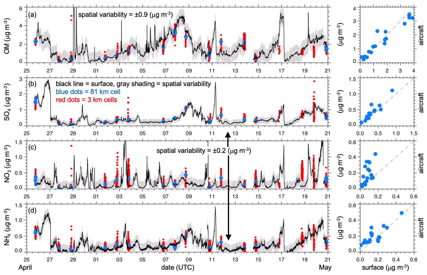
Figure 11Measured (a) OM, (b) SO4, (c) NO3, and (d) NH4 at the surface SGP site during IOP 1 (black lines), along with aircraft 81 km cell averages within the boundary-layer (blue dots) and 3 km cell averages (red dots) with the 81 km cell over the SGP site. The right-hand-side panels compare coincident-in-time surface and aircraft measurements.
Figure 12 is similar to Fig. 11, except that the temporal variations from surface CPC3025, CPC 3010, Scanning Mobility Particle Sizer (SMPS), and CCN are shown. The gray shading denotes the range of spatial variability indicated by the maximum departures from zero for the 5th and 95th percentile aircraft data shown in Fig. 8, which is 55 % for the CPC3025 and CP3010, 52 % for SMPS, and 28 % for CCN. Unfortunately, ground CCN data are not available prior to 10 May, so that those measurements can only be compared with eight flights during IOP 1.
While the aircraft measurements reveal large spatial variations in aerosol number concentrations around the SGP site as reflected by the range of 3 km cell means in Fig. 12a–c, it is interesting that the 81 km cell means are frequently very similar to the surface measurements. The temporal variations in CCN shown in Fig. 12d are similar to the OM concentrations in Fig. 11a. As with the number concentrations, the aircraft 81 km cell means for CCN are similar to the ground measurements after 10 May.

Figure 12Measured (a) number concentration >3 nm, (b) number concentration >10 nm, (c) number concentration between 1 and 972 nm, and (d) CCN concentration at the surface SGP site during IOP 1 (black lines), along with aircraft 81 km cell averages within the boundary-layer (blue dots) and 3 km cell averages (red dots) with the 81 km cell over the SGP site. The right-hand-side panels compare coincident-in-time surface and aircraft measurements.
When comparing observations with model predictions, it is important to note that “resolution” of spatial variability of an atmospheric variable and “grid spacing” have different meanings (Pielke et al., 1991; Grasso, 2000). A minimum of four to six grid spacings is required to resolve variations in physical features, but the exact number is subjective (Durran, 2000), and more grid spacings are preferable to fully resolve those features. Nevertheless, many modeling studies still incorrectly use “resolution” and “grid spacing” interchangeably. In relation to the findings from this study, coarse climate models with grid spacings greater than a quarter of a degree will not adequately resolve the spatiotemporal variability in aircraft measurements of aerosol properties around the SGP site. However, their predictions of aerosol properties may agree reasonably well with aircraft measurements averaged over the coarse model grid cells. Conversely, operational forecasting models and research chemical transport models with kilometer-scale grid spacings will resolve much, but not all, of the spatiotemporal variability since a 3 km grid spacing can only resolve variations that are at a minimum of four to six grid spacings wide (i.e., 12 to 18 km).
While the statistics shown in Sect. 4 describe the spatial variability of aerosol properties in terms of all the flights over a month-long IOP, the amount of spatial variability in aerosol properties varied from day to day. For example, some days had more or less spatial variability in aerosol composition, as shown by the flight on 7 May in Fig. 3b. As shown in Fig. 11, the range of OM 3 km cell means around the SGP site was smaller on other days (e.g., 25 April) than on 7 May. In contrast, 7 May also had little spatial variability in SO4 compared with other days.
Aircraft sampling during HI-SCALE had many repeatable flight patterns over the same region to characterize the day-to-day spatial variability, but the number of flights still can be considered limited for defining typical spatial variability. Our results also indicate seasonal differences in spatial variability which may not be applicable to conditions during the fall and winter months. While there have been many aircraft missions of aerosol properties over the past several decades, many of them have not had repeatable transects over a small region that can be used to characterize spatial variability. For example, flights during the Studies of Emissions and Atmospheric Composition, Clouds, and Climate Coupling by Regional Surveys (SEAC4RS, Toon et al., 2016) campaign were conducted over much of the continental US; therefore, most of the measurements can only quantify spatial variability once over a specific region. Nevertheless, it may be possible to characterize spatial variability in the vicinity of Houston, with the highest density of flight tracks where the research aircraft were based. Several campaigns have also been conducted in Houston, including the TexAQS 2000 and 2006 campaigns (Brock et al., 2003; Parish et al., 2009) among others, so that compiling measurements of aerosol properties from those campaigns may provide more robust estimates of variability that could also change in time as aerosol precursor emissions change. SENEX (Warneke et al., 2016) is another campaign that conducted grid-like aircraft flight paths over urban regions in the southeastern US; however, most of the urban areas were sampled only once. While subgrid-scale variability statistics similar to those in this study could be computed from those transects, the statistics would not be robust since they would depend on meteorological conditions and chemical evolution for a particular day.
It is also important to note that weather and climate models often have poor vertical resolution in addition to coarse grid spacings, which impacts our concept of subgrid-scale variability. For example, large vertical gradients in aerosol properties are frequently observed across the top of the boundary layer and lower troposphere, which requires small grid spacings on the order of tens of meters to resolve adequately. It is possible that aircraft measurements could be used to quantify subgrid-scale variability associated with vertical gradients; however, this aspect was not explored in this study since there were relatively few profiles made by the G-1 aircraft during HI-SCALE compared with the time spent on horizontal transects. In addition, vertical profiles usually extended to just above the boundary-layer top, so that vertical gradients in aerosol properties across a large portion of the lower troposphere were not characterized. Other aircraft datasets may be more appropriate for this purpose (e.g., Wang et al., 2020). In the future, unmanned aerial platforms that can operate for longer periods of time may have sufficient measurements to provide robust statistics on vertical gradients in aerosol properties.
In this study, we use aerosol properties measured by research aircraft during the 2016 HI-SCALE field campaign over northern–central Oklahoma near the DOE ARM Southern Great Plains site to quantify their subgrid-scale variability over a range of spatial scales. Aerosol properties examined include bulk composition concentrations, composition derived from a single-particle mass spectrometer, aerosol number concentrations, aerosol size distribution, and CCN concentrations. To compute subgrid-scale variability statistics, the aircraft flight paths are divided into segments that fall within grid cells that are 81, 27, 9, and 3 km wide. The coarser and finer grid spacings are consistent with those used by current global climate and operational forecasting models, respectively. Only the constant-altitude flight legs within the convective boundary layer are used to minimize variations associated with the vertical gradients in aerosol properties. Day-to-day variations in mean aerosol properties are also removed from the statistics to isolate variations due solely to spatial variability. Multiple aircraft flights occurred over the same region, so that more robust statistics of subgrid-scale variability could be obtained. The seasonality of subgrid-scale variability in aerosol properties is quantified by comparing the statistics from the spring and late-summer periods. In addition, we explore the representativeness of surface point measurements at the SGP site by comparing the variability of aerosol properties in the boundary layer with that at the ground.
Not surprisingly, we find that the coarse 81 km cell averages miss substantial variability in aerosol composition, mixing state, number, size distribution, and CCN over the SGP site. Even though this site is in a rural area, relatively large variations in aerosol properties are produced because of local variations in anthropogenic and biogenic precursor emissions and chemical formation superimposed on background aerosols transported from upwind regions. We also show the following.
-
The subgrid-scale variability associated among the 27 km cells is qualitatively similar to the distribution obtained from the 9 and 3 km cells. This does not imply that global climate models with ∼ 0.25∘ grid spacings are capable of resolving the observed aerosol variability at the SGP because a minimum of four to six grid cells are needed to resolve spatial variations in atmospheric constituents. Therefore, smaller grid spacings consistent with current operational forecasting models are likely needed to explicitly represent the observed spatial variability in aerosol properties.
-
As shown in Fig. 5, 90 % of the 27, 9, and 3 km cell mean OM concentrations varied by as much as 46 % of the 81 km cell mean around the SGP site. Similar statistics for SO4 and NO3 produced lower (as much as 35 % different) and higher (as much as 64 % different) spatial variability, respectively, than OM.
-
90 % of the 27, 9, and 3 km cell mean accumulation-mode number concentrations varied from the 81 km mean by as much as 35 %. The spatial variability in number concentrations that included ultrafine and Aitken-mode particles was larger, producing variations as large as 68 % of the 81 km cell mean. Much of this variability was due to local sources of ultrafine particles close to and downwind of the Redrock Power Plant and Ponca City Refinery and more widespread NPF events during IOP 1.
-
The spatial variability of some composition species and particles of less than 50 nm in diameter has skewed distributions.
-
Analyses of the variations in size distributions (Fig. 9) reveal that the 81 km cell mean is often quite different from the variability of the 3 km cell means over the SGP site. This suggests that coarse climate models may misrepresent CCN concentrations because subgrid-scale variability in size distribution is neglected. Averaging observed size distribution variations can also hide bimodal distributions that reflect chemical processes contributing to particle growth.
-
Even the 3 km cell averages miss extreme local maxima and minima in aerosol properties, especially for number concentrations of small particles.
-
Even though there are large variations in aerosol properties around the rural SGP site, we find that the 81 km averages of the aircraft properties are often very close to the ground measurements made at a single point. The exception is NO3, but since NO3 concentrations are usually low during HI-SCALE, those differences do not seem to significantly impact comparisons of average aircraft and surface aerosol number and CCN. This suggests that coarse global model predictions of aerosol properties can be directly compared with SGP site measurements. However, it would be useful to account for the range of observed variability derived from the aircraft measurements to indicate how much local variability the model does not represent, similar to accounting for measurement uncertainties that complicate measurement-to-model comparisons.
In terms of seasonal differences in subgrid-scale variability, we found the following.
-
Spatial variability in OM in terms of absolute differences with the 81 km mean (Fig. S5) increased from spring to late summer rather than during the spring, but the percentage differences (Fig. 5) had smaller seasonal dependence. This suggests that the higher concentrations themselves during IOP 2 contributed to the increased variability of absolute differences. The higher OM concentrations during the late summer likely resulted from higher SOA formation rates coupled with variability in both anthropogenic and biogenic precursor sources.
-
In contrast to OM, both absolute concentrations (Fig. S5) and percentage differences (Fig. 5) of NO3 had more variability during IOP 1. The lower variability during IOP 2 was due to both lower concentrations and more uniformly distributed NO3.
-
Analyses of the composition classes derived from a single-particle mass spectrometer suggest more complex seasonal differences than bulk composition measurements. While there were relatively small differences between IOPs 1 and 2 for many mixtures of organics, fresh OM (Org 1) and aged OM (Org 2) had less spatial variability during the summer. During IOP 1, the majority of organics were from biomass burning or were mixed with sulfate and nitrate with relatively lower and spatially more variable concentrations of pure organic-rich particles. During IOP 2, OM was composed primarily of organic-rich particles that were less variable over the SGP site.
-
Consistent with the bulk OM composition measurements, the spatial variability in the absolute differences in mean accumulation-mode aerosol number (Fig. S8) between the 27, 9, and 3 km cells and the 81 km cell mean was larger during the late summer, while the percentage differences (Fig. 8) did not vary much between IOPs 1 and 2. Even though IOP 1 had more frequent NPF events, the spatial variability in ultrafine and Aitken-mode particles was larger during IOP 2. While there were large variations in total number concentrations during IOP1, average concentrations were also higher in general during IOP 1, so that the overall spatial variability was larger during IOP 2.
-
Seasonal differences in the spatial variability of CCN were also consistent with the variability associated with bulk composition and accumulation-mode aerosol number, with little seasonal differences in terms of percentage differences with the 81 km cell mean (Fig. 10) and larger spatial variability in the absolute differences during IOP 2 (Fig. S10).
The methodology of computing subgrid-scale aerosol variability statistics could be extended to other aircraft campaigns with repeated flight tracks over a particular region. For example, past G-1 aircraft missions over Mexico City (Kleinman et al., 2008), Cape Cod (Berg et al., 2016), and Sacramento (Zaveri et al., 2012) and downwind of Manaus, Brazil (Shilling et al., 2018), are potential candidates that can be used to quantify subgrid-scale variability directly over and just downwind of large urban areas. While the magnitude of aerosol concentrations and the footprint from urban sources likely change over the years due to growth and/or emission controls, these datasets would provide an estimate of spatial variability influenced by meteorological conditions that are likely similar from year to year. For aerosols in a more remote continental region, the recent Cloud, Aerosol, and Complex Terrain Interactions (CACTI) field campaign (Varble et al., 2021) provided repeated aerosol measurements over a limited area that would be useful for assessing how subgrid-scale variabilities in aerosol properties influence the life cycle of deep convection.
In addition to providing alternative methods of evaluating model predictions, such information derived from aircraft field campaigns could also be used to develop numerical treatments that consider subgrid-scale aerosol variability in aerosol–cloud–radiation interactions in conjunction with existing treatments of cloud parameterizations.
Data used in this paper are available from the ARM data archive https://www.arm.gov/research/campaigns/sgp2016hiscale (DOE, 2022).
The supplement related to this article is available online at: https://doi.org/10.5194/acp-22-11217-2022-supplement.
JDF performed the data analyses and prepared the manuscript with contributions from JES, JL, AZ, DMB, KS, FM, JT, GS, and RZ. JES and JL are the mentors of the AMS instrument, AZ, DMB, and KS are mentors of the miniSPLAT instrument, JW is the instrument mentor of the FIMS instrument, and FM and JT are mentors of the CPC and CCN instrumentation on the G-1 aircraft. GS contributed to the analysis producing the particle class information based on the miniSPLAT measurements.
The contact author has declared that none of the authors has any competing interests.
Publisher’s note: Copernicus Publications remains neutral with regard to jurisdictional claims in published maps and institutional affiliations.
The HI-SCALE field campaign was supported by the Atmospheric Radiation Measurement (ARM) Climate Research Facility and the Environmental Molecular Sciences Laboratory (EMSL) through projects 48804 and 49297. Both are U.S. Department of Energy (DOE) Office of Science User Facilities sponsored by the Office of Biological and Environmental Research. The ground deployment of an HR-ToF-AMS was supported by the EMSL. We thank Tamara Pinterich for operating the FIMS instrument during HI-SCALE. This research was supported by the Atmospheric System Research (ASR) program as part of the DOE Office of Biological and Environmental Research under PNNL project KP1701010/57131. Pacific Northwest National Laboratory is operated by the DOE by the Battelle Memorial Institute under contract DE-A06-76RLO 1830.
This research has been supported by the U.S. Department of Energy (grant no. KP1701010/57131).
This paper was edited by Yuan Wang and reviewed by two anonymous referees.
Aaron, M. C, Dick, W. D., and Romay, F. J.: A new coincidence correction method for condensation particle counters, Aerosol Sci. Tech., 47, 177–182, https://doi.org/10.1080/02786826.2012.737049, 2013.
Albrecht, B. A.: Aerosols, cloud microphysics, and fractional cloudiness, Science, 245, 1227–1230, https://doi.org/10.1126/science.245.4923.1227. 1989.
Anderson, T. L., Charlson, R. J., Winker, D. M., Ogren, J. A., and Holmen, K.: Mesoscale variations of tropospheric aerosols, J. Atmos. Sci., 60, 119–136, https://doi.org/10.1175/1520-0469(2003)060<0119:MVOTA>2.0.CO;2, 2003.
Arakawa, A. and Schubert, W. H.: Interaction of a cumulus cloud ensemble with the large-scale environment, Part I, J. Atmos. Sci., 31, 675–701, https://doi.org/10.1175/1520-0469(1974)031<0674:IOACCE>2.0.CO;2, 1974.
Asher, E., Thornberry, T., Fahey, D. W., McComiskey, A., Carslaw, K., Grunau, S., Change, K.-L., Telg, H., Chen, P., and Gao, R.-S.: A novel network-based approach to determining measurement representation error for model evaluation of aerosol microphysical properties, J. Geophys. Res., 127, e2021JD035485, https://doi.org/10.1029/2021JD035485, 2022.
Barron, N. R., Ryan, S. D., and Heus, T.: Reconciling chord length distributions and area distributions for fields of fractal cumulus clouds, Atmosphere, 11, 824, https://doi.org/10.3390/atmos11080824, 2021.
Berg, L. K., Fast, J. D., Barnard, J. C., Burton, S. P., Cairns, B., Chand, D., Comstock, J. M., Dunagan, S., Ferrare, R. A., Flynn, C. J., Hair, J. W., Hostetler, C. A., Hubbe, J., Johnson, R., Kassianov, E. I., Kluzek, C. D., Mei, F., Miller, M. A., Michalsky, J., Ortega, I., Pekour, M., Rogers, R. R., Russell, P. B., Redemann, J., Sedlacek III, A. J., Segal-Rosenheimer, M., Schmid, B., Shilling, J. E., Shinozuka, Y., Springston, S. R., Tomlinson, J., Tyrrell, M., Wilson, J. M., Volkamer, R., Zelenyuk, A., and Berkowitz, C. M.: The Two-Column Aerosol Project: Phase I overview and impact of elevated aerosol layers on aerosol optical depth, J. Geophys. Res., 121, 336–361, https://doi.org/10.1002/2015JD023848, 2016.
Boucher, O., Randall, D., Artaxo, P., Bretherton, C., Feingold, G., Forster, P., Kerminen, V.-M., Kondo, Y., Liao, H., Lohmann, U., Rasch, P., Satheesh, S.K., Sherwood, S., Stevens, B., and Zhang, X. Y.: “Clouds and Aerosols”, in: Climate Change 2013: The Physical Science Basis. Contribution to Working Group I to the Fifth Assessment Report of the Intergovernmental Panel on Climate Change, edited by: Stocker, T. F., Qin, D., Plattner, G.-K., Tignor, M., Allen, S. K., Boschung, J., Nauels, A., Xia, Y., Bex, V., and Midgley, P. M., United Kingdom and New York, NY, USA, Cambridge University Press, https://doi.org/10.1017/CBO9781107415324.016, 2013.
Brock, C. A., Trainer, M., Ryerson, T. B., Neuman, J. A., Parrish, D. D., Holloway, J. S., Nicks Jr., D. K., Frost, G. J., Hübler, G., Fehsenfeld, F. C., Wilson, J. C., Reeves, J. M., Lafleur, B. G., Hilbert, H., Atlas, E. L., Donnelly, S. G., Schauffler, S. M., Stroud, V. R., and Wiedinmyer, C.: Particle growth in urban and industrial plumes in Texas, J. Geophys. Res., 108, 4111, https://doi.org/10.1029/2002JD002746, 2003.
Brock, C. A., Williamson, C., Kupc, A., Froyd, K. D., Erdesz, F., Wagner, N., Richardson, M., Schwarz, J. P., Gao, R.-S., Katich, J. M., Campuzano-Jost, P., Nault, B. A., Schroder, J. C., Jimenez, J. L., Weinzierl, B., Dollner, M., Bui, T., and Murphy, D. M.: Aerosol size distributions during the Atmospheric Tomography Mission (ATom): methods, uncertainties, and data products, Atmos. Meas. Tech., 12, 3081–3099, https://doi.org/10.5194/amt-12-3081-2019, 2019.
DeCarlo, P. F., Kimmel, J. R., Trimborn, A., Northway, M. J., Jayne, J. T., Aiken, A. C., Gonin, M., Fuhrer, K., Horvath, T., Docherty, K. S. Worsnop, D. R., and Jimenez, J. L.: Field-deployable, high-resolution, time-of-flight aerosol mass spectrometer, Anal. Chem., 78, 8281–8289, https://doi.org/10.1021/ac061249n, 2006.
DeMott, P. J., Prenni, A. J. Liu, X., Kreidenweis, S. M., Petters, M. D., Twohy, C. H., Richardson, M. S., Eidhammer, T., and Rogers, D. C.: Predicting global atmospheric ice nuclei distributions and their impacts on climate, P. Natl. Acad. Sci. USA, 107, 11217–11222, https://doi.org/10.1073/pnas.0910818107, 2010.
DOE: ARM HI-SCALE data, DOE [data set], https://www.arm.gov/research/campaigns/sgp2016hiscale, last access: 30 August 2022.
Durran, D. R.: Comments on “The differentiation between grid spacing and resolution and their application to numerical modeling”, Bull. Am. Meteorol. Soc., 81, 2478, https://doi.org/10.1175/1520-0477(2000)081<2478:COTDBG>2.3.CO;2, 2000.
Dusek, U., Frank, G. P., Hildebrandt, L., Curtius, J., Schneider, J., Walter, S., Chand, D., Drewnick, F., Hings, S., Jung, D., Borrmann, S., and Andreae, M. O.: Size matters more than chemistry for cloud-nucleating ability of aerosol particles, Science, 312, 1375–1378, https://doi.org/10.1126/science.1125261, 2006.
Ekman, A. M. L. and Rodhe, H.: Regional temperature response due to indirect sulfate aerosol forcing: Impact of model resolution, Clim. Dynam., 21, 1–10, https://doi.org/10.1007/s00382-003-0311-y, 2003.
Fast J. D., Berg, L. K., Alexander, L., Bell, D., D'Ambro, E., Hubbe, J., Kuang, C., Liu, J., Long, C., Matthews, A., Mei, F., Newsom, R., Pekour, M., Pinterich, T., Schmid, B., Schobesberger, S., Shilling, J., Smith, J., Springston, S., Thornton, J. A., Tomlinson, J., Wang, J., Xiao, H., and Zelenyuk, A.: Overview of the HI-SCALE field campaign: A new perspective on shallow convective clouds, Bull. Am. Meteorol. Soc., 100, 821–840, https://doi.org/10.1175/BAMS-D-18-0030.1, 2019.
Golaz, J.-C., Larson, V. E., and Cotton, W. R.: A PDF-based-model for boundary layer clouds. Part I: Method and model description, J. Atmos. Sci., 59, 3540–3551, https://doi.org/10.1175/1520-0469(2002)059<3540:APBMFB>2.0.CO;2, 2002.
Grasso, L. D.: The differentiation between grid spacing and resolution and their application to numerical modeling, Bull. Am. Meteorol. Soc., 3, 579–580, https://doi.org/10.1175/1520-0477(2000)081<0579:CAA>2.3.CO;2, 2000.
Griewank, P. J., Heus, T., Lareau, N. P., and Neggers, R. A. J.: Size dependence in chord characteristics from simulated and observed continental shallow cumulus, Atmos. Chem. Phys., 20, 10211–10230, https://doi.org/10.5194/acp-20-10211-2020, 2020.
Guenther, A. B., Jiang, X., Heald, C. L., Sakulyanontvittaya, T., Duhl, T., Emmons, L. K., and Wang, X.: The Model of Emissions of Gases and Aerosols from Nature version 2.1 (MEGAN2.1): an extended and updated framework for modeling biogenic emissions, Geosci. Model Dev., 5, 1471–1492, https://doi.org/10.5194/gmd-5-1471-2012, 2012.
Gustafson Jr., W. I., Qian, Y., and Fast, J. D.: Downscaling aerosols and the impact of neglected sub-grid processes on aerosol radiative forcing for a representative GCM grid spacing, J. Geophys. Res., 116, D13303, https://doi.org/10.1029/2010JD015480, 2011.
Kaufman, Y. J., Tanré, D., and Boucher, O.: A satellite view of aerosols in the climate system, Nature, 419, 215–223, https://doi.org/10.1038/nature01091, 2002.
Kleinman, L. I., Springston, S. R., Daum, P. H., Lee, Y.-N., Nunnermacker, L. J., Senum, G. I., Wang, J., Weinstein-Lloyd, J., Alexander, M. L., Hubbe, J., Ortega, J., Canagaratna, M. R., and Jayne, J.: The time evolution of aerosol composition over the Mexico City plateau, Atmos. Chem. Phys., 8, 1559–1575, https://doi.org/10.5194/acp-8-1559-2008, 2008.
Krishnamurthy, R., Newsom, R. K., Berg, L. K., Xiao, H., Ma, P.-L., and Turner, D. D.: On the estimation of boundary layer heights: a machine learning approach, Atmos. Meas. Tech., 14, 4403–4424, https://doi.org/10.5194/amt-14-4403-2021, 2021.
Liu, J., Alexander, L., Fast, J. D., Lindenmaier, R., and Shilling, J. E.: Aerosol characteristics at the Southern Great Plains site during the HI-SCALE campaign, Atmos. Chem. Phys., 21, 5101–5116, https://doi.org/10.5194/acp-21-5101-2021, 2021.
Ma, P.-L., Rasch, P. J., Fast, J. D., Easter, R. C., Gustafson Jr., W. I., Liu, X., Ghan, S. J., and Singh, B.: Assessing the CAM5 physics suite in the WRF-Chem model: implementation, resolution sensitivity, and a first evaluation for a regional case study, Geosci. Model Dev., 7, 755–778, https://doi.org/10.5194/gmd-7-755-2014, 2014.
Szopa, S., Naik, V., Adhikary, B., Artaxo, P., Berntsen, T., Collins, W. D., Fuzzi, S., Gallardo, L., Kiendler-Scharr, A., Klimont, Z., Liao, H., Unger, N., and Zanis, P.: “Short-lived climate forcers”, in: AR6 Climate Change 2021: The Physical Science Basis. Contribution to Working Group I to the Sixth Assessment Report of the Intergovernmental Panel on Climate Change, edited by: Masson-Delmotte, V., Zhai, P., Pirani, A., Connors, S. L., Peìan, C., Berger, S., Caud, N., Chen, Y., Goldfarb, L., Gomis, M. I., Huang, M., Leitzell, K., Lonnoy, E., Matthews, J. B. R., Maycock, T. K., Waterfield, T., Yelekçi, O., Yu, R., and Zhou, B., Cambridge University Press, https://doi.org/10.1017/9781009157896.008, 2021.
Parrish, D. D., Allen, D. T., Bates, T. S., Estes, M., Fehsenfeld, F. C., Feingold, G., Ferrare, R., Hardesty, R. M., Meagher, J. F., Nielsen-Gammon, J. W., Pierce, R. B., Ryerson, T. B., Seinfeld, J. H., and Williams, E. J.: Overview of the Second Texas Air Quality Study (TexAQS II) and the Gulf of Mexico Atmospheric Composition and Climate Study (GoMACCS), J. Geophys. Res., 114, D00F13, https://doi.org/10.1029/2009JD011842, 2009.
Patel, P. N. and Jiang, J. H.: Cloud condensation nuclei characteristics at the Southern Great Plains site: role of particle size distribution and aerosol hygroscopicity, Environ. Res. Comm., 3, 076002, https://doi.org/10.1088/2515-7620/ac0e0b, 2021.
Petters, M. D. and Kreidenweis, S. M.: A single parameter representation of hygroscopic growth and cloud condensation nucleus activity, Atmos. Chem. Phys., 7, 1961–1971, https://doi.org/10.5194/acp-7-1961-2007, 2007.
Pielke, R. A.: A recommended specific definition of “resolution”, Bull. Am. Meteorol. Soc., 72, 1914, https://doi.org/10.1175/1520-0477-72.12.1914, 1991.
Pöhlker, M. L., Pöhlker, C., Ditas, F., Klimach, T., Hrabe de Angelis, I., Araújo, A., Brito, J., Carbone, S., Cheng, Y., Chi, X., Ditz, R., Gunthe, S. S., Kesselmeier, J., Könemann, T., Lavrič, J. V., Martin, S. T., Mikhailov, E., Moran-Zuloaga, D., Rose, D., Saturno, J., Su, H., Thalman, R., Walter, D., Wang, J., Wolff, S., Barbosa, H. M. J., Artaxo, P., Andreae, M. O., and Pöschl, U.: Long-term observations of cloud condensation nuclei in the Amazon rain forest – Part 1: Aerosol size distribution, hygroscopicity, and new model parametrizations for CCN prediction, Atmos. Chem. Phys., 16, 15709–15740, https://doi.org/10.5194/acp-16-15709-2016, 2016.
Qian, Y., Gustafson Jr., W. I., and Fast, J. D.: An investigation of the sub-grid variability of trace gases and aerosols for global climate modeling, Atmos. Chem. Phys., 10, 6917–6946, https://doi.org/10.5194/acp-10-6917-2010, 2010.
Ren, J., Zhang, F., Wang, Y., Collins, D., Fan, X., Jin, X., Xu, W., Sun, Y., Cribb, M., and Li, Z.: Using different assumptions of aerosol mixing state and chemical composition to predict CCN concentrations based on field measurements in urban Beijing, Atmos. Chem. Phys., 18, 6907–6921, https://doi.org/10.5194/acp-18-6907-2018, 2018.
Rosenfeld, D., Andreae, M. O., Asmi, A., Chin, M., de Leeuw, G., Donovan, D. P., Kahn, R., Kinne, S., Kivekäs, N., Kulmala, M., Lau, W., Schmidt, K. S., Suni, T., Wagner, T., Wild, M., and Quaas, J.: Global observations of aerosol-cloud-precipitation-climate interactions, Rev. Geophys., 52, 750–808, https://doi.org/10.1002/2013RG000441, 2014.
Ryerson, T. B., Andrews, A. E., Angevine, W. M., Bates, T. S., Brock, C. A., Cairns, B., Cohen, R. C., Cooper, O. R., de Gouw, J. A., Fehsenfeld, F. C., Ferrare, R. A., Fischer, M. L., Flagan, R. C., Goldstein, A. H., Hair, J. W., Hardesty, R. M., Hostetler, C. A., Jimenez, J. L., Langford, A. O., McCauley, E., McKeen, S. A., Molina, L. T., Nenes, A., Oltmans, S. J., Parrish, D. D., Pederson, J. R., Pierce, R. B., Prather, K., Quinn, P. K., Seinfeld, J. H., Senff, C. J., Sorooshian, A., Stutz, J., Surratt, J. D., Trainer, M., Volkamer, R., Williams, E. J., and Wofsy, S. C.: The 2010 California Research at the Nexus of Air Quality and Climate Change (CalNex) field study, J. Geophys. Res., 118, 5830–5866, https://doi.org/10.1002/jgrd.50331, 2013.
Schmid, B., Tomlinson, J. M., Hubbe, J. M., Comstock, J. M., Mei, F., Chand, D., Pekour, M. S., Kluzek, C. D., Andrews, E., Biraud, S. C., and McFarquhar, G. M.: The DOE ARM Aerial Facility, Bull. Am. Meteorol. Soc., 95, 723–742, https://doi.org/10.1175/BAMS-D-13-00040.1, 2014.
Schutgens, N., Tsyro, S., Gryspeerdt, E., Goto, D., Weigum, N., Schulz, M., and Stier, P.: On the spatio-temporal representativeness of observations, Atmos. Chem. Phys., 17, 9761–9780, https://doi.org/10.5194/acp-17-9761-2017, 2017.
Shilling, J. E., Pekour, M. S., Fortner, E. C., Artaxo, P., de Sá, S., Hubbe, J. M., Longo, K. M., Machado, L. A. T., Martin, S. T., Springston, S. R., Tomlinson, J., and Wang, J.: Aircraft observations of the chemical composition and aging of aerosol in the Manaus urban plume during GoAmazon 2014/5, Atmos. Chem. Phys., 18, 10773–10797, https://doi.org/10.5194/acp-18-10773-2018, 2018.
Sisterson, D. L., Peppler, R. A., Cress, T. S., Lamb, P. J., and Turner, D. D.: The ARM Southern Great Plains (SGP) site, The Atmospheric Radiation Measurement (ARM) program: The first 20 years, Meteorological Monograph, Bull. Am. Meteorol. Soc., 57, 6.1–6.14, https://doi.org/10.1175/AMSMONOGRAPHS-D-16-0004.1, 2016.
Toon, O. B., Maring, H., Dibb, J., Ferrare, R., Jacob, D. J., Jensen, E. J., Luo, Z. J., Mace, G. G., Pan, L. L., Pfister, L., Rosenlof, K. H., Redemann, J., Reid, J. S., Singh, H. B., Thompson, A. M., Yokelson, R., Minnis, P., Chen, G., Jucks, K. W., and Pszenny, A.: Planning, implementation, and scientific goals of the Studies of Emissions and Atmospheric Composition, Clouds and Climate Coupling by Regional Surveys (SEAC4RS) field mission, J. Geophys. Res., 121, 4967–5009, https://doi.org/10.1002/2015JD024297, 2016.
Tucker, S. C., Senff, C. J., Weickmann, A. M., Brewer, W. A., Banta, R. M., Sandberg, S. P., Law, D. C., and Hardesty, R. M.: Doppler lidar estimation of mixing height using turbulence, shear, and aerosol profiles, J. Atmos. Ocean. Tech., 26, 673–688, https://doi.org/10.1175/2008JTECHA1157.1, 2009.
Twomey, S.: Pollution and the planetary albedo, Atmos. Environ., 8, 1251–1256, https://doi.org/10.1016/0004-6981(74)90004-3, 1974.
Varble, A. C., Nesbitt, S. W. Salio, P., Hardin, J. C., Bharadwaj, N., Borque, P., DeMott, P. J., Feng, Z., Hill, T. C. J., Marquis, J. N., Matthews, A., Mei, F., Öktem, R., Castro, V., Goldberger, L., Hunzinger, A., Barry, K. R., Kreidenweis, S. M., McFarquhar, G. M., McMurdie, L. A., Pekour, M., Powers, H., Romps, D. M., Saulo, C., Schmid, B., Tomlinson, J. M., van den Heever, S. C., Zelenyuk, A., Zhang, Z., and Zipser, E. J.: Utilizing a storm-generating hotspot to study convective cloud transitions: The CACTI experiment, Bull. Am. Meteorol. Soc., 102, E1597–E1620, https://doi.org/10.1175/BAMS-D-20-0030.1, 2021.
Wainwright, C. D., Pierce, J. R., Liggio, J., Strawbridge, K. B., Macdonald, A. M., and Leaitch, R. W.: The effect of model spatial resolution on Secondary Organic Aerosol predictions: a case study at Whistler, BC, Canada, Atmos. Chem. Phys., 12, 10911–10923, https://doi.org/10.5194/acp-12-10911-2012, 2012.
Wang, J.: Effects of spatial and temporal variations in aerosol properties on mean cloud albedo, J. Geophys. Res., 112, D16201, https://doi.org/10.1029/2007jd008565, 2007.
Wang, Y., Pinterich, T., and Wang, J.: A fast integrated mobility spectrometer with wide dynamic size range: Theoretical analysis and numerical simulation, Rapid measurement of sub-micrometer aerosol size distribution using a fast integrated mobility spectrometer, J. Aerosol Sci. 121, 12–20, https://doi.org/10.1016/j.jaerosci.2018.03.006, 2018.
Wang, Y., Zheng, X., Dong, X., Xi, B., Wu, P., Logan, T., and Yung, Y. L.: Impacts of long-range transport of aerosols on marine-boundary-layer clouds in the eastern North Atlantic, Atmos. Chem. Phys., 20, 14741–14755, https://doi.org/10.5194/acp-20-14741-2020, 2020.
Warneke, C., Trainer, M., de Gouw, J. A., Parrish, D. D., Fahey, D. W., Ravishankara, A. R., Middlebrook, A. M., Brock, C. A., Roberts, J. M., Brown, S. S., Neuman, J. A., Lerner, B. M., Lack, D., Law, D., Hübler, G., Pollack, I., Sjostedt, S., Ryerson, T. B., Gilman, J. B., Liao, J., Holloway, J., Peischl, J., Nowak, J. B., Aikin, K. C., Min, K.-E., Washenfelder, R. A., Graus, M. G., Richardson, M., Markovic, M. Z., Wagner, N. L., Welti, A., Veres, P. R., Edwards, P., Schwarz, J. P., Gordon, T., Dube, W. P., McKeen, S. A., Brioude, J., Ahmadov, R., Bougiatioti, A., Lin, J. J., Nenes, A., Wolfe, G. M., Hanisco, T. F., Lee, B. H., Lopez-Hilfiker, F. D., Thornton, J. A., Keutsch, F. N., Kaiser, J., Mao, J., and Hatch, C. D.: Instrumentation and measurement strategy for the NOAA SENEX aircraft campaign as part of the Southeast Atmosphere Study 2013, Atmos. Meas. Tech., 9, 3063–3093, https://doi.org/10.5194/amt-9-3063-2016, 2016.
Weigum, N. M., Stier, P., Schwarz, J. P., Fahey, D. W., and Spackman, J. R.: Scales of variability of black carbon plumes over the Pacific Ocean, Geophys. Res. Lett., 399, L15804, https://doi.org/10.1029/2012GL052127, 2012.
Weigum, N., Schutgens, N., and Stier, P.: Effect of aerosol subgrid variability on aerosol optical depth and cloud condensation nuclei: implications for global aerosol modelling, Atmos. Chem. Phys., 16, 13619–13639, https://doi.org/10.5194/acp-16-13619-2016, 2016.
Wiedinmyer, C., Akagi, S. K., Yokelson, R. J., Emmons, L. K., Al-Saadi, J. A., Orlando, J. J., and Soja, A. J.: The Fire INventory from NCAR (FINN): a high resolution global model to estimate the emissions from open burning, Geosci. Model Dev., 4, 625–641, https://doi.org/10.5194/gmd-4-625-2011, 2011.
Wofsy, S. C., Daube, B., Jimenez, R., Kort, E., Pittman, J. V., Park, S., Commane, R., Xiang, B., Santoni, G., Jacob, D., Fisher, J., Pickett-Heaps, C., Wang, H., Wecht, K. J., Wang, Q.-Q., Stephens, B. B., Shertz, S., Romashkin, P., Campos, T., Haggerty, J., Cooper, W. A., Rogers, D., Beaton, S., Hendershot, R., Elkins, J. W., Fahey, D., Gao, R., Moore, F., Montzka, S. A., Schwarz, J., Hurst, D., Miller, B., Sweeney, C., Oltmans, S., Nance, D., Hintsa, E., Dutton, G., Watts, L., Spackman, R., Rosenlof, K., Ray, E., Zondlo, M. A., Diao, M., Keeling, R., Bent, J., Atlas, E., Lueb, R., Mahoney, M. J., Chahine, M., Olson, E., Patra, P., Ishijima, K., Engelen, R., Flemming, J., Nassar, R., Jones, D. B. A., and Fletcher, S. E. M.: HIAPER Pole-to-Pole Observations (HIPPO): Fine-grained, global scale measurements of climatically important atmospheric gases and aerosols, Philos. T. R. Soc. Lond. A, 369, 2073–2086, https://doi.org/10.1098/rsta.2010.0313, 2011.
Zaveri, R. A., Shaw, W. J., Cziczo, D. J., Schmid, B., Ferrare, R. A., Alexander, M. L., Alexandrov, M., Alvarez, R. J., Arnott, W. P., Atkinson, D. B., Baidar, S., Banta, R. M., Barnard, J. C., Beranek, J., Berg, L. K., Brechtel, F., Brewer, W. A., Cahill, J. F., Cairns, B., Cappa, C. D., Chand, D., China, S., Comstock, J. M., Dubey, M. K., Easter, R. C., Erickson, M. H., Fast, J. D., Floerchinger, C., Flowers, B. A., Fortner, E., Gaffney, J. S., Gilles, M. K., Gorkowski, K., Gustafson, W. I., Gyawali, M., Hair, J., Hardesty, R. M., Harworth, J. W., Herndon, S., Hiranuma, N., Hostetler, C., Hubbe, J. M., Jayne, J. T., Jeong, H., Jobson, B. T., Kassianov, E. I., Kleinman, L. I., Kluzek, C., Knighton, B., Kolesar, K. R., Kuang, C., Kubátová, A., Langford, A. O., Laskin, A., Laulainen, N., Marchbanks, R. D., Mazzoleni, C., Mei, F., Moffet, R. C., Nelson, D., Obland, M. D., Oetjen, H., Onasch, T. B., Ortega, I., Ottaviani, M., Pekour, M., Prather, K. A., Radney, J. G., Rogers, R. R., Sandberg, S. P., Sedlacek, A., Senff, C. J., Senum, G., Setyan, A., Shilling, J. E., Shrivastava, M., Song, C., Springston, S. R., Subramanian, R., Suski, K., Tomlinson, J., Volkamer, R., Wallace, H. W., Wang, J., Weickmann, A. M., Worsnop, D. R., Yu, X.-Y., Zelenyuk, A., and Zhang, Q.: Overview of the 2010 Carbonaceous Aerosols and Radiative Effects Study (CARES), Atmos. Chem. Phys., 12, 7647–7687, https://doi.org/10.5194/acp-12-7647-2012, 2012.
Zaveri R. A., Wang, J., Fan, J., Zhang, Y., Shilling, J. E., Zelenyuk, A., Mei, F., Newsom, R., Pekour, M., Tomlinson, J., Comstock, J. M., Shrivastava, M., Fortner, E., Machado, L. A. T., Artaxo, P., and Martin, S. T.: Rapid growth of air pollution nanoparticles and their impacts on clouds in the Amazon rainforest, Sci. Adv., 8, eabj0329, https://doi.org/10.1126/sciadv.abj0329, 2022.
Zelenyuk, A., Imre, D., Wilson, J., Zhang, Z., Wang, J., and Mueller, K.: Airborne single particle mass spectrometers (SPLAT II and miniSPLAT) and new software for data visualization and analysis in a geo-spatial context, J. Am. Soc. Mass Spectr., 26, 257–270, https://doi.org/10.1007/s13361-014-1043-4, 2015.
- Abstract
- Introduction
- HI-SCALE aircraft measurements
- Defining subgrid-scale variability
- Spatial variability as a function grid spacing and season
- Discussion
- Summary and conclusions
- Data availability
- Author contributions
- Competing interests
- Disclaimer
- Acknowledgements
- Financial support
- Review statement
- References
- Supplement