the Creative Commons Attribution 4.0 License.
the Creative Commons Attribution 4.0 License.
 | 01 Sep 2022
Tropospheric and stratospheric ozone profiles during the 2019 TROpomi vaLIdation eXperiment (TROLIX-19)
John T. Sullivan
Arnoud Apituley
Nora Mettig
Karin Kreher
K. Emma Knowland
Marc Allaart
Ankie Piters
Michel Van Roozendael
Pepijn Veefkind
Jerry R. Ziemke
Natalya Kramarova
Mark Weber
Alexei Rozanov
Laurence Twigg
Grant Sumnicht
Thomas J. McGee
A TROPOspheric Monitoring Instrument (TROPOMI) validation campaign was held in the Netherlands based at the CESAR (Cabauw Experimental Site for Atmospheric Research) observatory during September 2019. The TROpomi vaLIdation eXperiment (TROLIX-19) consisted of active and passive remote sensing platforms in conjunction with several balloon-borne and surface chemical (e.g., ozone and nitrogen dioxide) measurements. The goal of this joint NASA-KNMI geophysical validation campaign was to make intensive observations in the TROPOMI domain in order to be able to establish the quality of the L2 satellite data products under realistic conditions, such as non-idealized conditions with varying cloud cover and a range of atmospheric conditions at a rural site. The research presented here focuses on using ozone lidars from NASA's Goddard Space Flight Center to better evaluate the characterization of ozone throughout TROLIX-19. Results of comparisons to the lidar systems with balloon, space-borne and ground-based passive measurements are shown. In addition, results are compared to a global coupled chemistry meteorology model to illustrate the vertical variability and columnar amounts of both tropospheric and stratospheric ozone during the campaign period.
- Article
(5073 KB) - Full-text XML
- BibTeX
- EndNote


In September 2019, a joint Royal Netherlands Meteorological Institute (KNMI) and US National Aeronautics and Space Administration (NASA) field campaign was performed in the Netherlands, based at the Cabauw Experimental Site for Atmospheric Research (CESAR, 51.97∘ N, 4.93∘ E), to provide the scientific community with additional information to further understand and evaluate the Copernicus Sentinel-5 Precursor mission (S-5P) TROPOspheric Monitoring Instrument (TROPOMI) instrument (https://sentinels.copernicus.eu/web/sentinel/missions/sentinel-5p, last access: 17 August 2022). The main objective of the Copernicus Sentinel-5P mission is to perform atmospheric measurements with high spatiotemporal resolution, to be used for scientific studies and monitoring of air quality and chemical transport (https://www.esa.int/Applications/Observing_the_Earth/Copernicus/Sentinel-5P, last access: 17 August 2022).
To properly support satellite evaluation, the 2019 TROpomi vaLIdation eXperiment (TROLIX-19) campaign was designed to bring together many active and passive remote sensing platforms in conjunction with several balloon-borne, airborne and surface measurements. Specifically, the observations were established to provide geophysical verification in order to establish the quality of TROPOMI Level 2 (L2) main data products under realistic non-idealized conditions with varying cloud cover and a wide range of atmospheric conditions. Cabauw, using its comprehensive in situ and remote sensing observation program in and around the 213 m meteorological tower (https://ruisdael-observatory.nl/trolix19-tropomi-validation-experiment-2019/, last access: 17 August 2022), was the main site of the campaign with a focus on vertical profiling using lidar instruments for aerosols, clouds, water vapor, tropospheric and stratospheric ozone, as well as balloon-borne sensors for nitrogen dioxide (NO2) and ozone (Fig. 1). Although this work focuses primarily on the ozone lidar profiling during the study, the larger campaign overview, background and motivation can be found in Apituley et al. (2019, 2020) or Kreher et al. (2020).
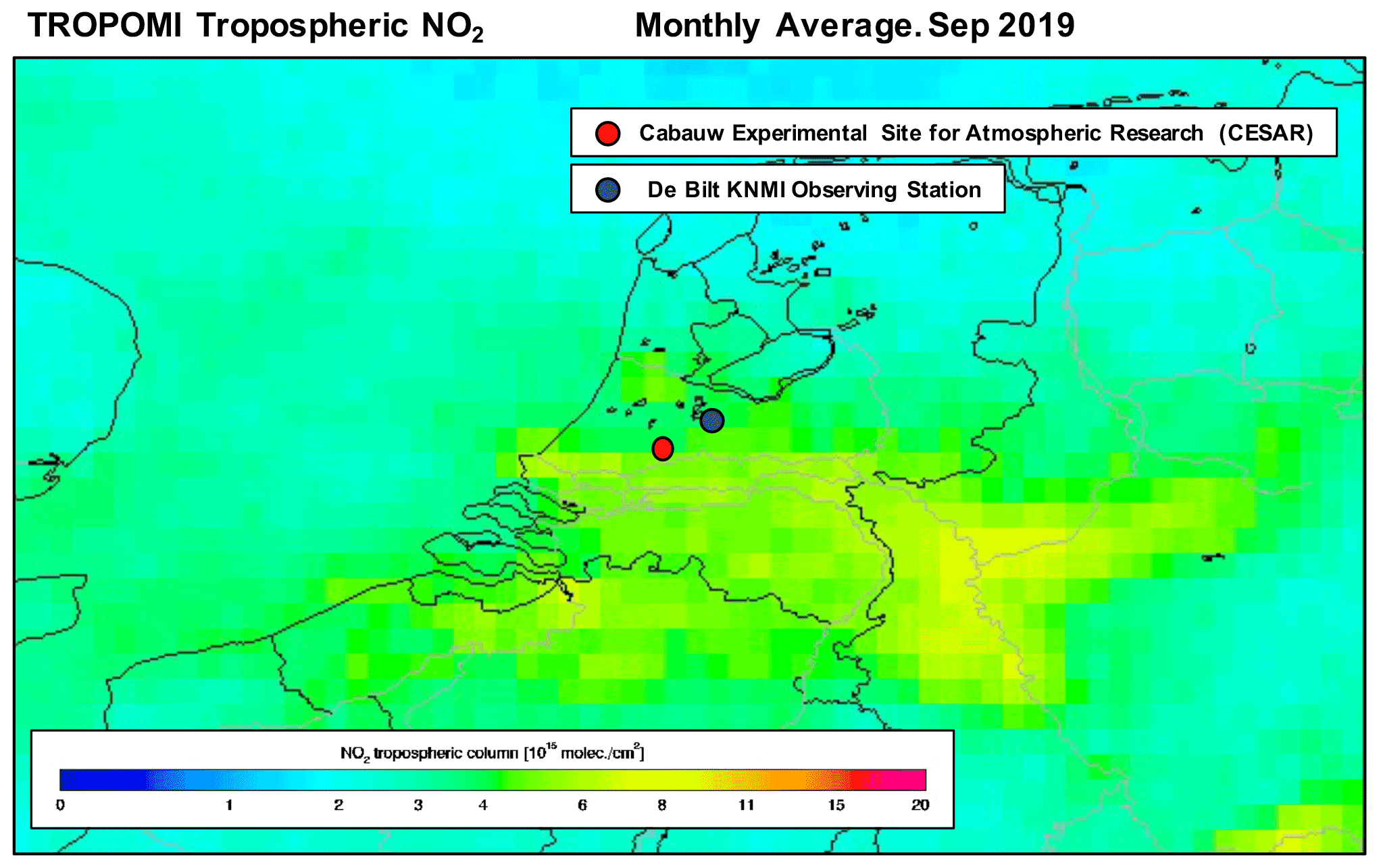
Figure 1TROPOMI monthly-mean tropospheric NO2 column (version 1.0) for September 2019. The CESAR and De Bilt, NL, sites are indicated in the image.
One main goal of this work is also to understand ozone profile retrievals as they relate to upcoming satellite endeavors. As NASA prepares to launch its first geostationary air quality satellite “Tropospheric Emissions: Monitoring of POllution” (TEMPO) this work also specifically establishes a paradigm of evaluation for TEMPO-derived products such as tropospheric ozone columns and a 0–2 km tropospheric ozone product. An analogous geo-stationary air quality satellite, the Copernicus Sentinel-4 mission (S-4, https://ruisdael-observatory.nl/trolix19-tropomi-validation-experiment-2019, last access: 17 August 2022), will provide hourly data on tropospheric constituents over Europe, and the CESAR site is directly within the satellite's field of regard. Due to the finer spatial footprint, increased temporal frequency and vertical extent of the TEMPO tropospheric ozone retrievals, ozone lidars are an ideal platform to perform future evaluations of the products, which builds from recent work done by Johnson et al. (2018). Specifically, this work will investigate the results from the combination of having a co-located NASA tropospheric (Sullivan et al., 2014) and stratospheric ozone lidars (McGee et al., 1991) in order to obtain an entire vertical profile of ozone from ∼0.2 to 50 km.
For the first time, this transportable combination of lidars is able to explicitly derive diurnally varying tropospheric and total ozone columns, which are compared directly to measurements obtained by ground-based passive sensors, current satellite instrumentation and chemical transport models. In Sect. 2 we present all available data and methods used in this work across the various platforms during the TROLIX-19 study. Section 3 focuses on comparisons of the tropospheric ozone retrievals of the vertical profiles of ozone within the troposphere and columnar reductions of 0–10 and 0–2 km. Comparisons of lidar data with available complete ozone profiles (Sect. 4) and columnar amounts (Sect. 5) from several platforms and chemical transport models are also presented to further understand the quality of satellite-derived ozone profiles during the TROLIX-19 period.
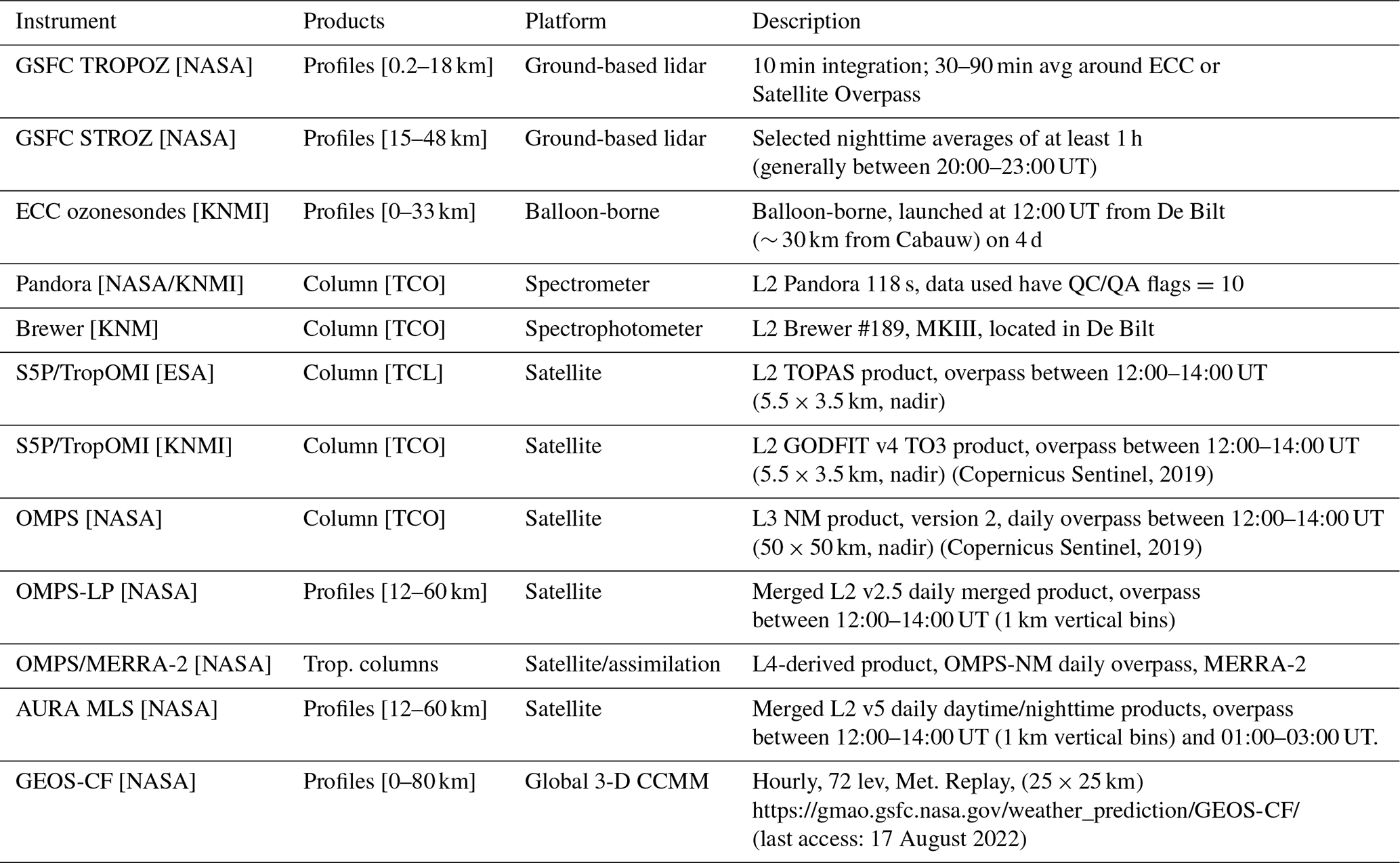
Descriptions of the various observational and model data sets used in this study are below, including a summary table (Table 1).
Table 1Instrument platforms, associated products and short description used in this work during the TROLIX-19 campaign.
2.1 NASA ozone differential absorption lidar (DIAL)
NASA deployed and operated two ozone lidars during TROLIX-19 at the Cabauw site near the CESAR tower to observe temporal and vertical gradients in tropospheric and stratospheric ozone. This was the first dual deployment of these lidars, in which the tropospheric ozone lidar measured between the near surface (about 0.2 km) to a height of about 18 km and the stratospheric lidar during nighttime from 15 km upwards to nearly 50 km, providing complete hybrid ozone profiles for the campaign period. Measurements were made during periods of mostly clear skies, although occasional cloud cover did enter the measurement period.
The NASA GSFC Mobile Stratospheric Ozone Lidar Trailer Experiment (STROZ-LITE) has been a participant in the Network for the Detection of Atmospheric Composition Change (NDACC) since its inception and is housed in a 12.5 m container allowing for transport around the world (McGee et al., 1991). The lidar instrument transmits two wavelengths, 308 nm from a XeCl excimer laser, and 355 nm from a ND:YAG laser to derive ozone number density profiles, which have historically served as an intercomparison data set for other NDACC ozone lidars (recent intercomparison can be found at Wing et al., 2020, 2021).
The NASA GSFC TROPOZ has been developed in a transportable 13.5 m trailer to take routine measurements of tropospheric ozone near the Baltimore–Washington, D.C. area as well as various campaign locations (Sullivan et al., 2014, 2015, 2019; Leblanc et al., 2018). This instrument, which utilizes a ND:YAG laser and Raman cell, has been developed as part of the ground-based Tropospheric Ozone Lidar NETwork (TOLNet, https://www-air.larc.nasa.gov/missions/TOLNet/, last access: 17 August 2022), which currently consists of stations across North America. The primary purposes of the instruments within TOLNet are to provide regular, high-fidelity profile measurements of ozone within the troposphere for satellite and model evaluation. This lidar also operates routinely for the Network for the Detection of Atmospheric Composition Change (NDACC).
More than 30 NDACC ground-based lidar instruments (https://lidar.jpl.nasa.gov/ndacc/index_ndacc.php, last access: 17 August 2022) deployed worldwide from pole to pole are monitoring atmospheric ozone, temperature, aerosols, water vapor and polar stratospheric clouds.
Both lidars collect backscattered radiation with a large primary telescope and a 10 cm telescope for near-field channels. Spectral separation is accomplished using dichroic beam-splitters and interference filters. For the stratospheric system, five return wavelengths are recorded: the two transmitted wavelengths, the nitrogen Raman scattered radiation from each of the transmitted beams 332 and 382 nm, and the 408 nm water vapor channel. In this arrangement for TROLIX-19, the tropospheric system pumped the Raman cell with the fourth harmonic (266 nm), which resulted in conversion to 289 and 299 nm using a single Raman cell with a mixture of hydrogen and deuterium. All of the signals are further split to improve the dynamic range of the respective lidar optical detection chains and are then amplified, discriminated and recorded using photon counting techniques.
During TROLIX-19, the STROZ-LITE was operated on cloud-free nights, with measurements lasting between 2–4 h to obtain enough signal to properly retrieve the entire stratospheric ozone profile. The TROPOZ was operated during daytime and nighttime to provide tropospheric ozone profiles. For instances of TROPOMI overpasses, campaign ozonesondes or coincident stratospheric ozone lidar measurements, the TROPOZ reported data are averaged for 30 min, centered around the satellite overpass or launch time. This temporal period of averaging has been optimized in several cases to avoid cloud contamination. For all other times during the TROPOZ operation, the data have been averaged to 10 min, which is suitable under most clear sky conditions to retrieve ozone information within the entire troposphere. A brief description and community standardized definitions of the uncertainty budget of the lidar measurements presented in this paper can be found in Sullivan et al. (2014), Leblanc et al. (2016, 2018). The maximum statistical uncertainties for the two GSFC lidars vary from night to night depending on atmospheric conditions and laser power fluctuations. They are mostly within 10 %–20 % for 5 min and 5 %–8 % for 30 min integrations throughout the atmosphere. Within overlapping measurement regions in the upper troposphere–lower stratosphere, they are different at the same altitude due to laser performance and telescope–detector efficiency differences and are therefore joined manually for this work based on appropriate signal to noise and uncertainty estimates.
2.2 Ground-based passive sensors and ozonesondes
2.2.1 Pandora spectrometer instrument
A Pandora spectrometer instrument (#118) has been used to measure columnar amounts of trace gases in the atmosphere at 3–5 min resolution at the Cabauw site since 2016 and was previously used for the second Cabauw Intercomparison of Nitrogen Dioxide (CINDI-2) campaign (Kreher et al., 2020). Using the theoretical solar spectrum as a reference, Pandora determines trace gas amounts using differential optical absorption spectroscopy (DOAS). This attributes in principal these differences in spectra measured by Pandora to the presence of trace gases within the atmosphere (i.e., the difference between the theoretical solar spectrum and measured spectrum is caused by absorption of trace gas species). For this study, L2 direct sun columnar values of ozone are used, although retrievals of nitrogen dioxide are also operationally acquired. Data used passed the strictest quality assurance estimate (flags = 10) and were obtained from the Pandonia Global Network (http://data.pandonia-global-network.org/, last access: 17 August 2022).
2.2.2 Brewer MKIII spectrophotometer
A Brewer MKIII spectrometer instrument (#189) has been used to measure daily columnar amounts of ozone in the atmosphere at the KNMI, De Bilt (30 km NE of Cabauw, 52.10∘ N, 5.18∘ E). Brewer #189 has been operated continuously since 1 October 2006. It replaced Brewer #100 which has provided observations since 1 January 1994. De Bilt has the longest continuous record of ozone measured with an MKIII instrument in the World Ozone and Ultraviolet Radiation Data Centre (WOUDC) database.
The Brewer is specifically designed to provide high-accuracy measurement of spectrally resolved UV for satellite evaluation, climatology monitoring and public health to international standards. Similar to Pandora spectrometers, ground-based columnar measurements of trace gases are derived by comparing the measured UV spectrum with known solar output and modeling the scattering properties of the atmosphere. Based on their long-term stability, they have been historically used to evaluate columnar satellite products (McPeters et al., 2007; Wenig et al., 2008; Garane et al., 2019). The Brewer is the standard instrument used in the World Meteorological Organization ozone monitoring network and for NDACC. These data were obtained at the NDACC website (https://www-air.larc.nasa.gov/missions/ndacc/data.html, last access: 17 August 2022).
2.2.3 Ozonesondes
Ozonesondes have been used to measure vertical profiles of ozone in the atmosphere at the KNMI, De Bilt (30 km NE of Cabauw), site since November 1992, and measurements are made weekly, historically at 12:00 UTC on Thursdays. Description of the Electro Chemical Cell (ECC) details and metadata are summarized in Van Malderen et al. (2016), which also describes the importance of understanding and reporting changes in ozonesonde operation procedures. During the campaign, in situ measurements of ozone were made using a balloon-borne payload consisting of an ECC ozonesonde (Science Pump Corporation, Serial Numbers: 6A35438, 6A35447, 6A35448, 6A35441) coupled with a radiosonde (Vaisala RS41) and have been used to evaluate TROPOMI tropospheric ozone products in the tropics (Hubert et al., 2021). The ECC technique is widely used for the high vertical resolution measurements of O3. The ECC consists of two chambers with platinum electrodes immersed in potassium iodide (KI) solutions at different concentrations. The accuracy in the O3 concentration measured by an ECC ozonesonde is ± 5%–10% up to an altitude of 30 km (Smit et al., 2007, 2021). These data were obtained at the NDACC website (https://www-air.larc.nasa.gov/missions/ndacc/data.html, last access: 17 August 2022).
2.3 Satellite observations and products
Satellite data used in this work were selected based on the closest retrieval (i.e., column, profile) to the CESAR station within ∘ latitude and ∘ longitude.
2.3.1 Ozone mapping and profiling suite (OMPS) and MERRA-2 products
The Ozone Mapping and Profiler Suite (OMPS) on the Suomi National Polar-orbiting Partnership (S-NPP) platform consists of three sensors to measure the total column and the vertical distribution of ozone with high spatial and vertical resolutions (Flynn et al., 2006). Daily total column ozone overpasses over Cabauw station from the OMPS Nadir-Mapper (NM) instrument are used in this study. The vertical distribution of ozone in the stratosphere and lower mesosphere is obtained from the OMPS Limb-Profiler (LP) sensor on the Suomi-NPP satellite merging the UV (29.5–52.5 km) and VIS (12.5–35.5 km) bands to provide a full profile from 12.5 to 52.5 km (Kramarova et al., 2018). Variations of this merged OMPS-LP retrieval were considered; however, the work shown in Arosio et al. (2018), indicates the same overall conclusions would be reached. Further work beyond this paper may involve comparing this TROLIX-19 measurement data set to specific experimentally performed satellite retrievals.
The Modern-Era Retrospective analysis for Research and Applications, Version 2 (MERRA-2), provides data beginning in 1980 and since August 2004 assimilates NASA's satellite ozone profile observations from the Aura Microwave Limb Sounder (MLS) (Livesey et al., 2008) to more comprehensively characterize stratospheric ozone abundance. A residual tropospheric ozone product (Ziemke et al., 2019) is derived using the OMPS NM total column ozone minus the co-located MERRA-2 stratospheric column ozone. Tropopause pressure is derived from MERRA-2 potential vorticity (2.5 PVU) and potential temperature (380 K).
2.3.2 MLS
NASA's Aura Microwave Limb Sounder (MLS) uses microwave emission to measure stratospheric and upper tropospheric constituents, such as ozone. Ozone data (v5) used in this study are binned on various vertical grids and are converted from volume mixing ratio to number density using the coincident MERRA-2 atmosphere state parameters. Both daytime and nighttime data are used in this study, and the corresponding closest profile is utilized for comparison.
2.3.3 TROPOMI
In October 2017, the Sentinel-5 Precursor (S5P) mission was launched, carrying the TROPOspheric Monitoring Instrument (TROPOMI), which is a nadir-viewing 108∘ field-of-view push-broom grating hyperspectral spectrometer. Starting in August 2019, Sentinel-5P TROPOMI along-track high spatial resolution (approximately 5.5 km at nadir) has been implemented and total ozone columns values used in this work are subsetted from the NASA GES DISC (https://tropomi.gesdisc.eosdis.nasa.gov/data/S5P_TROPOMI_Level2/S5P_L2__O3_TOT_HiR.1/, last access: 17 August 2022) to provide the Offline 1-Orbit L2 (S5P_L2__O3_TOT_HiR), which is based on the direct-fitting algorithm (S5P_TO3_GODFIT), comprising a non-linear least squares inversion by comparing the simulated and measured backscattered radiances.
Tropospheric Ozone vertical profiles were retrieved using the TOPAS (Tikhonov regularized Ozone Profile retrievAl with SCIATRAN) algorithm and were applied to the TROPOMI L1B spectral data version 2, using spectral data between 270 and 329 nm for the retrieval (Mettig et al., 2021). This data set will cover the TROLIX-19 period from 9–28 September; however, it is available outside of this work for specific weeks between June 2018 and October 2019. Since the ozone profiles are very sensitive to absolute calibration at short wavelengths, a re-calibration of the measured radiances is required using comparisons with simulated radiances with ozone limb profiles from collocated satellites used as input. The a priori profiles for ozone are taken from the ozone climatology of Lamsal et al. (2004), and the calibration correction spectrum is determined using the radiances modeled with ozone information from collocated Aura MLS measurements as described in depth throughout Mettig et al. (2021).
2.4 Coupled chemistry and meteorology model
The GEOS Composition Forecasting (GEOS-CF, https://gmao.gsfc.nasa.gov/weather_prediction/GEOS-CF/ (last access: 17 August 2022), Keller et al., 2021; Knowland et al., 2021) system was chosen to serve as a comparison simulation for this effort, based on its altitude coverage (up to 80 km) and implications for future geostationary satellite use. The system produces global, three-dimensional distributions of atmospheric composition with a spatial resolution of 25 km. Using meteorological analyses from other GEOS systems, the GEOS-CF products include a running atmospheric replay to provide near-time estimates of surface pollutant distributions and the composition of the troposphere and stratosphere. Individual case study evaluations using ozone lidar of the GEOS-CF meteorological replay have recently been performed in Dacic et al. (2020), Gronoff et al. (2021) and Johnson et al. (2021). These results will also be used to better evaluate the GEOS-CF as the source of a priori ozone profiles for use in the TEMPO tropospheric ozone retrievals. Model output for this work is used from the closest GEOS-CF model grid cell to the CESAR observatory.
3.1 Vertical profiles
Example tropospheric ozone profile observations are presented in Fig. 2 for seven individual observation periods during the TROLIX-19 campaign. Each of the panels show the cloud screened TROPOZ lidar retrievals (top panels) and the corresponding GEOS-CF model output (bottom panels). Pink dots are overlaid to indicate the simulated tropopause altitude based on a blended estimate (TROPPB) which meets criteria of the lowest altitude bin corresponding with either a pressure level above the thermal tropopause (380 K) or dynamical (3 PVU) tropopause.
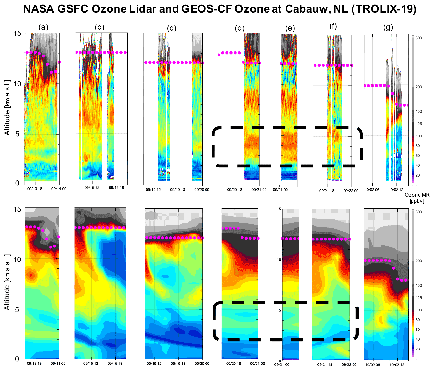
Figure 2Cloud screened TROPOZ lidar retrievals (top panels) and the corresponding GEOS-CF model output (bottom panels) from the closest model grid cell to the CESAR observatory during TROLIX-19 for (a) 13 September at 14:00–00:00 UTC, (b) 15 September at 09:00–21:00 UTC, (c) 19 September at 10:00–00:00 UT, (d) 20 September at 16:00–00:00 UT, (e) 21 September at 00:00–03:00 UT, (f) 21 September at 16:00–00:00 UT and (g) 2 October at 04:00–14:00 UT. Pink dots are overlaid to indicate the simulated tropopause altitude based on a blended estimate (TROPPB).
In general, the observations and simulations agree quite well in characterizing the broad features that impacted the CESAR site during the TROLIX-19 campaign. However, in each panel there are ozone laminae within the lower troposphere that are not replicated in the model simulation, most notably the underestimation of ozone during the 20–21 September period from 3–5 km (Fig. 2d–f, black dashed box). However, the model does simulate well the lowered tropopause height and abundance of lower stratospheric ozone observed in the 2 October observations (see Fig. 2g), which is an indication of the model representing the dynamical variability that affects the lowering of the tropopause height. This suggests the model is appropriately capturing the complex dynamics during this period near the upper troposphere but may not have been initialized with the correct boundary conditions or is too spatially coarse to allow for simulation of the layer emphasized with the black dashed box. However, this is an important altitude region for identifying long-range transport of aged stratospheric air and inter-continental transport that may be downward mixing towards the surface layer and will be explored in more detail below.
To bring in additional platforms and to better understand these differences throughout the campaign at discrete altitudes, Fig. 3 shows the ozone number density values for the TROPOZ lidar, GEOS-CF model, TROPOMI and ECC ozonesondes at the average 4 km vertical level for the entire TROLIX-19 campaign period. Within this layer, the platforms are all characterizing the general ozone features throughout the campaign at an altitude that frequently is associated with aged transported laminae. There is a noticeable difference between the observations and model during the previously described 20–21 September period. On 21 September at 12:00 UT, the lidar and ECC sonde quantify an elevated layer (1.2–1.3 × 10²¹ molec. m−3) into the region that is not simulated by model (0.75–0.9 ×10²¹ molec. m−3), resulting in an approximately 30 % underestimation in ozone abundance within the layer.
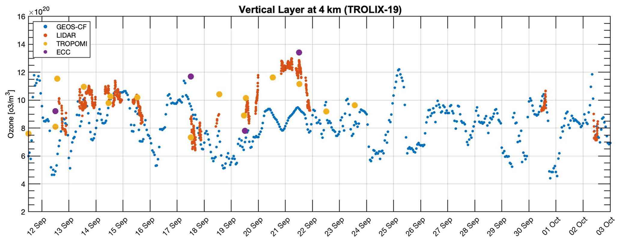
Figure 3Ozone number density values for the TROPOZ lidar, GEOS-CF mode, TROPOMI and electro-chemical cell (ECC) ozonesondes at the 4 km layers. The layer was calculated to match the closest representative vertical layer of the GEOS-CF for consistent intercomparison. Data are averaged in a 500 m layer from 3.94 to 4.44 km a.g.l.
3.2 Columnar data reduction
There continues to be a need within the atmospheric and satellite community to understand the variability of ozone as it pertains to both the tropospheric column (i.e., the Earth's surface to the tropopause height) and the 0–2 km tropospheric column (i.e., the Earth's surface to the 2 km height). The 0–2 km region is of particular interest as it is projected to be delivered hourly from the North American geo-stationary satellite – Tropospheric Emissions: Monitoring of Pollution (TEMPO). Due to the increased temporal frequency and vertical extent of TEMPO's tropospheric ozone retrievals, ozone lidars, such as those from TOLNet (https://www-air.larc.nasa.gov/missions/TOLNet/, last access: 17 August 2022) used in this work, are an ideal platform to perform future evaluations of the products.
Full tropospheric columns (Fig. 4a) are consistently calculated from each platform using the blended tropopause height (TROPPB) produced by the GEOS-CF and described above (see pink dots in Fig. 2) and are then converted to Dobson units (DU). The tropospheric and 0–2 km columns are calculated explicitly by integrating the ozone number density from the lowest data bin of usable data to the TROPPB or 2 km layer height produced in the nearest model temporal output. The exception to this is the OMPS/MERRA-2 tropospheric column using the residual method described above (subtracting the MERRA-2 stratospheric column from the OMPS-NM total ozone column).
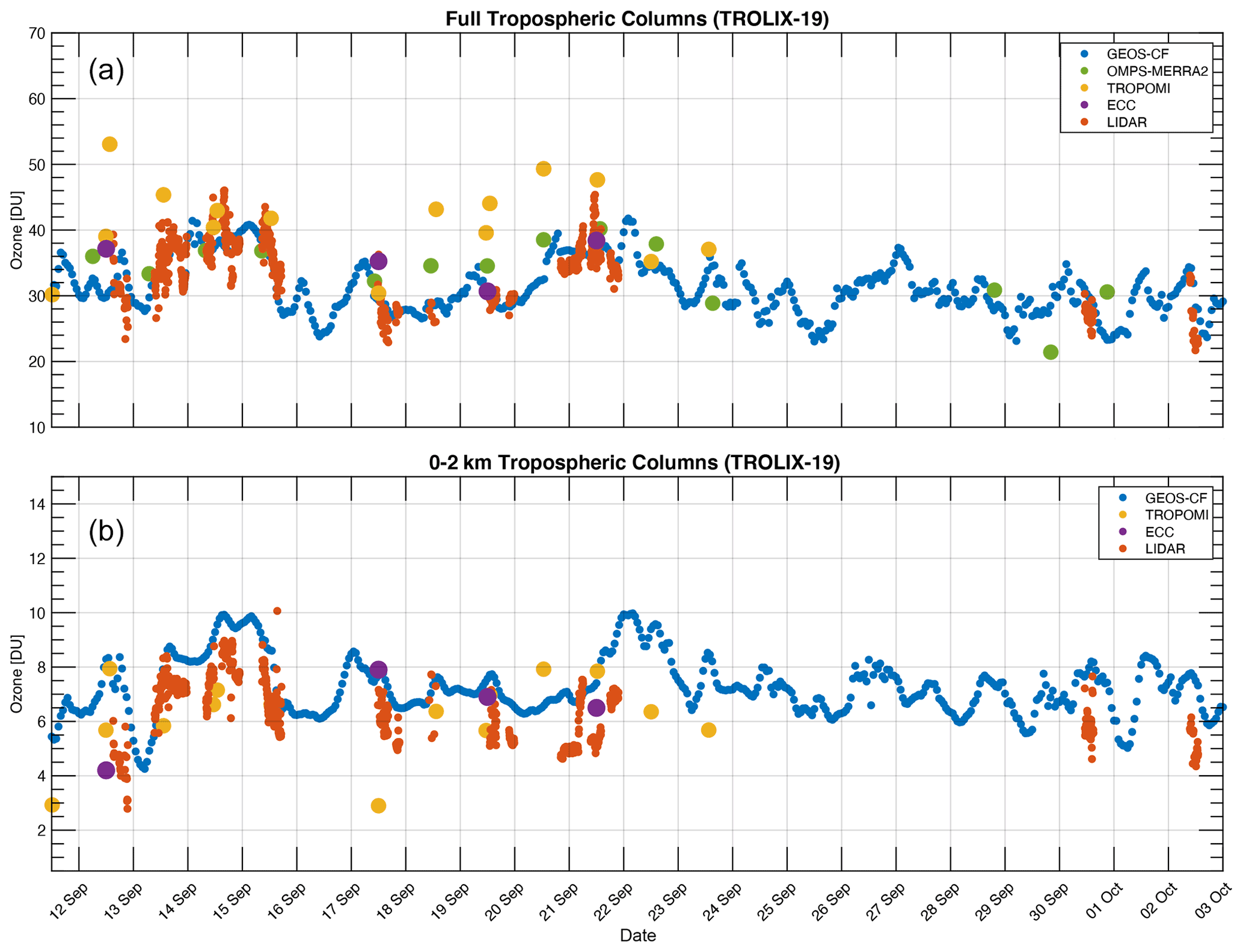
Figure 4Full tropospheric columns (a) and 0–2 km tropospheric columns (b) calculated from GEOS-CF, OMPS-MERRA2 (full column only), TROPOMI, lidar and ECC. Data where reflectivity was greater than 0.6 were excluded to remove cloud interference.
For the full tropospheric column (Fig. 4a), the campaign variability ranges from approximatively 20–55 DU based on the lidar observations. The model, lidar and ECC sonde observations agree quite well throughout the 12–23 September time frame when looking at day-to-day variability. However, when assessing the variability on a single day for 21 September, full tropospheric columns reduced from the lidar observations are some of the largest observed during this TROLIX-19 period (reaching 46 DU), though they mostly stay between 34–40 DU. During this time, the model mainly ranges between 35–37 DU, resulting in differences within 10 % for most of the observations (albeit closer to 30 % for the peak on this day).
When looking at Fig. 2d–f, the lower ozone values just below the tropopause during this period are not simulated in the model, which may be an indication that the mesoscale ozone transport in the frontal system is not very well resolved by the model for this specific event. Since the model correctly simulated many other ozone features during this time period within the upper tropospheric region, this may also be attributed to aged transport into the domain that was not available during model initialization. Back-trajectories were performed to better identify the sources of these air masses; however, nothing conclusive can be reported. The layer is not associated with any increase in lidar attenuated backscatter within the associated altitude, suggesting it was not urban in origin and therefore more likely aged stratospheric air mixing down to the lower free troposphere. Outside of this 21 September period, there is generally good agreement between the observations (including the OMPS-MERRA2 product) and model, indicating the combination of observations and modeling is able to represent the rural conditions and ozone perturbations at the CESAR site.
When assessing these tropospheric column values from the TROPOMI ozone profile observations, it is important to mention the vastly different vertical resolution or averaging kernel schemes as compared to the independent observations near the tropopause. The ECC samples an instantaneous observation with a vertical resolution generally less than 100 m, while the lidar is averaging over 500–750 m of atmosphere for each data point near the tropopause. However, the vertical resolution near the tropopause for TROPOMI using the TOPAS algorithm (Mettig et al., 2021) is nearly 6 km, indicating it is not able to completely represent sharp gradients that may occur near the tropopause layer and the lower stratosphere (where ozone content sharply increases). This lack of degrees of independent information is evident in the relatively higher TROPOMI tropospheric column ozone values as compared to the other independent measurements presented in this work. This suggests ground-based profiling observations are still critically needed to confirm large deviations from a priori and climatology in order to evaluate the atmospheric chemistry models, especially in the upper tropospheric region and within the boundary layer.
There exists both diurnal and day-to-day variability of the 0–2 km ozone, ranging from 4–10 DU (Fig. 4b). In the 0–2 km ozone reduction, the lidar and model are critically needed to understand ozone variability on a continuous scale. For instance, on 15 September the 0–2 km ozone column was near 9 DU at 03:00 UT and finished near 5.5 DU at 16:00 UT, resulting in a −60 % change in DU within 13 h. The need for continuous measurements during highly variable days are further emphasized by the fact that this gradient in 0–2 km ozone for this single day (15 September, 5.5–9 DU) was comparable to the variance of 0–2 km ozone values throughout the entire campaign.
In summary, we find that the ozone columns evaluated in this study generally reproduced the structure of the TROLIX-19 ozone lidar observations for N=835 coincidences. For the full tropospheric column, the lidar calculated median was 30.9±4.7 DU, compared to 33.4±3.9 DU for the GEOS-CF. This indicates a difference of 2.5 DU or 7.9 %, which is well within the lidar uncertainty of around 10 % throughout the tropospheric column, and as we described above is likely driven by select days rather than an overall bias between the measurements. For the 0–2 km tropospheric column, the lidar calculated median was 5.8 DU ± 0.9 DU, compared to 7.8 DU ± 0.7 DU for the corresponding GEOS-CF measurements. For the TROLIX-19 campaign, a 0–2 km tropospheric column accounts for approximately 20 % of the tropospheric column as detailed in Fig. 4a, indicating measurements above the surface are critically needed to understand ozone variability at rural sites such as Cabauw, NL, where free tropospheric ozone features dominate the column.
4.1 Hybrid tropospheric–stratospheric ozone comparisons
To better understand differences in ozone retrievals from multiple platforms, it is important to assess the entire vertical distribution of ozone. To characterize the vertical distribution throughout the entire troposphere and stratosphere, hybrid ozone profiles were created from longer (integrations of 60–120 min vs. 10 min in Sect. 3) temporal retrievals from the closed co-located daytime–nighttime TROPOZ and nighttime STROZ lidar data, which were then interpolated to the GEOS-CF model vertical grid levels. Figure 5 compares these results to the GEOS-CF, OMPS-LP, TROPOMI, MLS and the ECC ozonesonde profiles for 12, 17, 19 and 21 September 2019. These days were selected as days within the campaign that had an ECC launch from De Bilt, NL (30 km from Cabauw).

Figure 5GEOS-CF, lidar, OMPS-LP, ECC, TROPOMI and MLS ozone profile comparisons for 12, 17, 19 and 21 September 2019. These days were selected as days within the campaign that had an ECC launch from De Bilt.
For each observation period in Fig. 5, all platforms manage to characterize a similar shape and extent of the ozone maxima between 2.5–4.5 molec. m−3 throughout the vertical layer between 20–25 km. In each case, there are differences between the platforms in characterizing the vertical variability and extent of the ozone maxima, which will be quantified in the following section. One notable feature that emphasizes the cross-platform ability to illustrate ozone variability in the stratosphere is from the 19 and 21 September profiles. A dual ozone maximum is observed quite remarkably by the merged lidar, ECC, MLS and OMPS-LP and simulated by the GEOS-CF centered around 20 km and then again at 25 km. The wind observations from the ozonesonde payload (not shown) indicate a wind shear within the two ozone layers, suggesting this feature was dynamically driven. The TROPOMI retrieval is not able to retrieve this vertical features due to its coarser vertical resolution and appears to average through the layers.
4.2 Difference profiles
To quantitatively compare the ozone retrievals and simulations, Fig. 6 displays the ozone values for the TROLIX-19 time period from the hybrid lidar data set (Fig. 6a), GEOS-CF (Fig. 6b), OMPS-LP (Fig. 6c), MLS (Fig. 6d) and TROPOMI (Fig. 6e). This double ozone maxima, starting after 20 September, serves as a geophysical marker to visually compare the ozone products. The lidar, model and OMPS-LP all capture this feature, but with varying ozone abundances and altitudes. From Fig. 6d, it appears as if TROPOMI retrievals are not able to resolve this feature. The percent differences, as compared to the lidar observations, are displayed in Fig. 7a–d. These percent differences are calculated using Eq. (1).
where E2 denotes the lidar observations and E1 denotes the respective ozone values from the various platforms in Fig. 6.
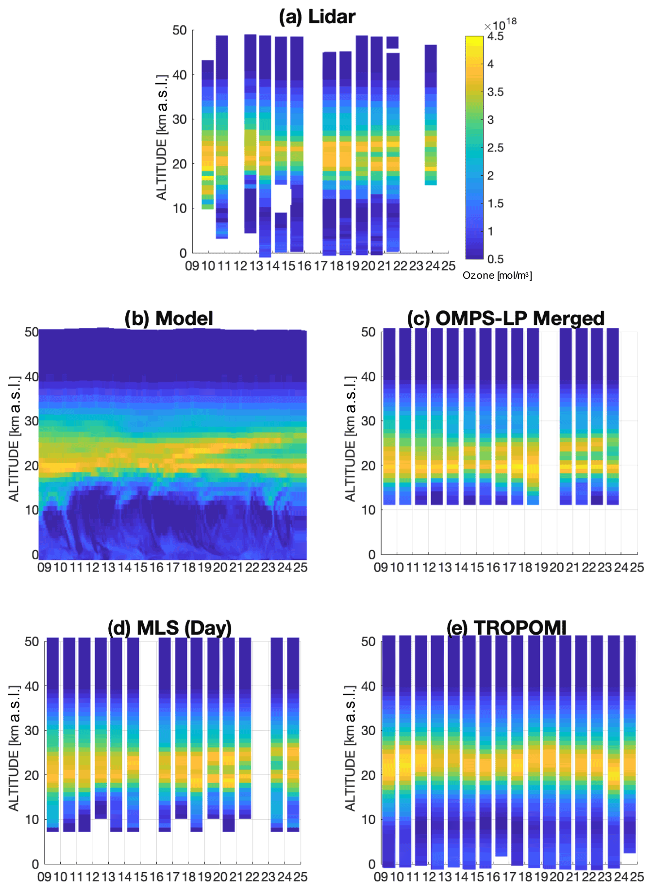
Figure 6Ozone number densities across all platforms for the TROLIX-19 time period from the hybrid lidar data set (a), GEOS-CF (b), OMPS-LP (c), MLS (d) and TROPOMI (e). The x axis is the day of September 2019.
The percent differences in Fig. 7a indicate the GEOS-CF model from 20–45 km generally represents the lidar observations, but they are generally 0 %–10 % lower in abundance. The percent differences in Fig. 7b indicate OMPS-LP is also representing the ozone maxima and altitude above 25 km. There are larger differences below 20 km, which indicates the OMPS-LP retrieval worsens (in both directions) as compared to the ozone abundance below 20 km as shown in the profiles in Fig. 5. The percent differences in Fig. 7c indicate the MLS data, especially those within the 20–40 km region, perform quite well as compared to the lidar observations. The percent differences in Fig. 7d indicate the TROPOMI retrieval is generally over-representing the ozone concentrations throughout the atmosphere, which worsens within the troposphere and has been discussed earlier for the tropospheric ozone column as a result of a much larger vertical resolution in this region. In all cases, the most variability in the differences occurs within the active region from 10–20 km that is driven by the dynamical tropopause height and lower stratospheric ozone abundance. Within each satellite data set, we find larger biases in the lower stratosphere and upper troposphere below 18 km, which has been previously described in the literature for the OMPS-LP data set in Kramarova et al. (2018) and were improved in the updated version 2.5 algorithm used in this work.
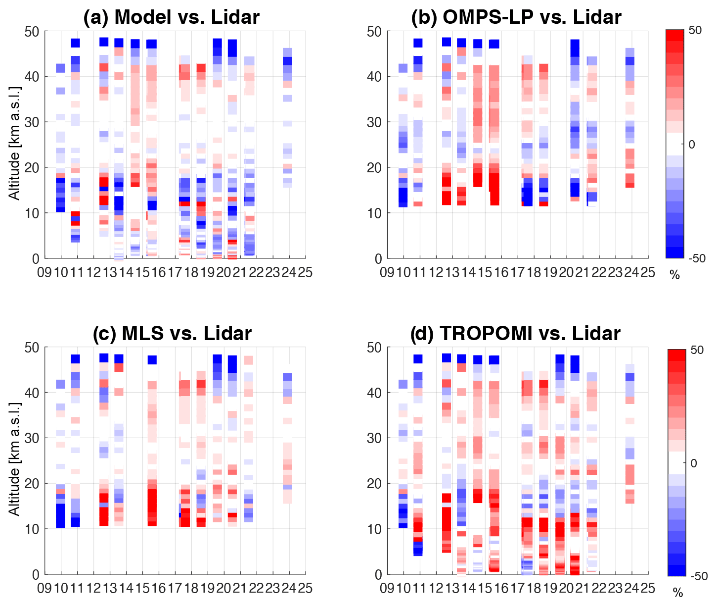
Figure 7Differences in ozone number densities across all platforms for the TROLIX-19 time period for the model (a), OMPS-LP (b), MLS (c) and TROPOMI (d). The x axis is the day of September 2019.
Similar to the troposphere, to better understand to what extent the vertical distribution of ozone impacts the atmospheric column, Fig. 8a shows the various platforms and their retrieved total column ozone. For this analysis, the GEOS-CF, lidar, OMPS-NM and TROPOMI (GODFIT) are shown, in addition to local ground-based measurements from a Pandora instrument and Brewer. The total column values range from 230–300 DU throughout the campaign period, with the median total column ozone of 271 DU. With the previous analyses from Sect. 3.2, this indicates the median total tropospheric column of 33 DU and 0–2 km boundary layer column of 6 DU results in percentages of the entire ozone column of 12 % and 2.3 %, respectively. Similar to the full tropospheric ozone columns, larger total ozone columns were observed towards the end of the TROLIX-19 period, suggesting this variability was partly due to a larger abundance of ozone in the lower stratosphere.
Figure 8b shows the various platforms as a percent differences from the model. In general, the various platforms are all mostly within 5 % of each other, with most differences being within ± 3 %. This analysis emphasizes the stability and maturity of the Pandora and Brewer systems for monitoring the total column ozone amounts. Interestingly, the double maxima feature in vertical ozone distribution in the stratosphere (with local minima between) described in Sect. 4.1 on 21 September does not severely impact the total column ozone.
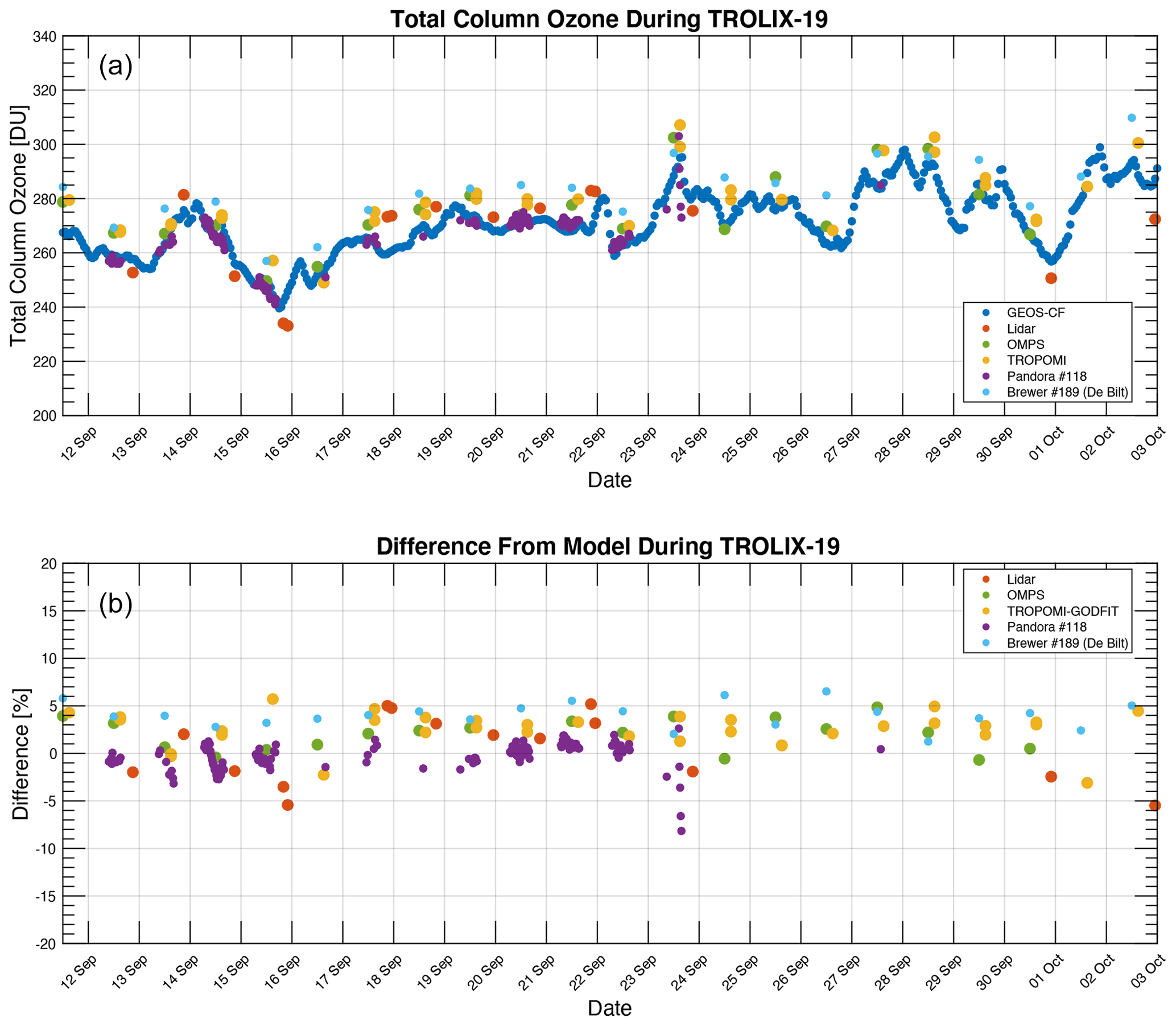
Figure 8Total ozone columns (a) and percent differences (b) as compared to the model observations for GEOS-CF, lidar, OMPS, TROPOMI, Pandora and Brewer.
This work has highlighted the various differences in retrieved ozone quantities during the TROLIX-19 campaign. This has emphasized the importance of ground-based ozone lidars and other measurements in understanding the vertical variability of ozone and how it relates to the column reduction. This work also shows the first effort to directly resolve both tropospheric columns and 0–2 km ozone columns from the NASA TROPOZ lidar. Other TOLNet lidars are able to perform this data reduction, and future work will be to expand this effort to the other TOLNet locations. This work indicates the level of performance of the GEOS-CF modeling system as compared to the other platforms, which ultimately performs extremely well both in the stratosphere (Figs. 6 and 7) and within the troposphere (Figs. 2 and 4).
One takeaway message or point of caution for future efforts is that although there are situations identified where the vertical profile and the model disagree in a certain altitude range (Fig. 3), when the data are reduced to a columnar product, compensating over- and underestimations may cancel out and produce a more accurate value when only looking at the results as compared to observations. For this reason, it is essential when doing data columnar reduction for the troposphere, and even more so in the 0–2 km column or planetary boundary layer, that observations of the vertical profile be used to evaluate the representativeness of the model and auxiliary data sets.
In looking towards the NASA TEMPO, this work indicates that the GEOS-CF, with its global coverage, hourly resolution and adequate vertical information to resolve most atmospheric features, is an appropriate choice for the a priori profiles for the TEMPO ozone retrievals. Continued investigations are needed with high-resolution observations, as presented in this work, to better evaluate the GEOS-CF, especially in these common transport regions of the atmosphere. Although the GEOS-CF performed well in reproducing the ozone downward transport throughout the upper troposphere and lower stratosphere, the model did fail to resolve some high-resolution laminae deeper into the lower troposphere related to specific mesoscale ozone transport in this region as evidenced in Figs. 2 and 3.
This work shows the TROPOMI TOPAS ozone profile algorithm products are able to accurately reproduce ozone quantities in the lower troposphere at various atmospheric levels. In particular, Figs. 3 and 4 show promising results that indicate the TROPOMI satellite observations compare well with the observations from ground-based measurements (lidar, sonde) of specific elevated ozone features. However, there is an observed overestimate of the TROPOMI retrieval in the upper troposphere and lower stratosphere (between 10 and 15 km) associated with a larger vertical resolution that needs to also be further evaluated to better understand the representativeness of the retrieval in this region, and efforts are underway to remedy this using combined-satellite retrievals (Mettig et al., 2022).
Figure 7 was presented as a quantitative resultant figure to illustrate both the temporal (i.e., throughout the course of the TROLIX-19 campaign) and vertical differences observed in the retrievals from each observational platform. This serves as a rare opportunity to cross-evaluate multiple satellite-based observations, a global chemical transport model, ozonesondes and a high-resolution ozone lidar suite. The authors feel that this figure has served to point out the strengths of each platform and present careful considerations for areas of under- or overestimation, Furthermore, we feel reducing these comparisons down to a specific percentage may underserve the community push for supporting the vertical profiling needed for these types of efforts.
The CESAR Observatory continues to be a critical landmark for campaigns that revolve around atmospheric composition measurements for satellite validation and evaluation beyond this effort, such as CINDI (Piters et al., 2012) and CINDI-2 (Kreher et al., 2020; Wang et al., 2020; Tirpitz et al., 2021). As the European Commission (EC) in partnership with the European Space Agency (ESA) continues to launch tropospheric composition satellites including the upcoming geo-stationary Sentinel-4 satellite, we expect this observatory will continue to host and maintain critical atmospheric sampling for future validation efforts.
The data used in the paper can be found at the following sources:
-
MLS ozone profiles can be downloaded from the NASA Goddard Space Flight Center Earth Sciences Data and Information Services Center (GES DISC; https://doi.org/10.5067/Aura/MLS/DATA2516, Schwartz et al., 2020).
-
The Pandora data are available at the Pandonia Global Network Archive (http://data.pandonia-global-network.org/Cabauw/) (Cede et al., 2020).
-
The OMPS LP version 2.5 ozone profiles can be downloaded from the NASA Goddard Space Flight Center Earth Sciences Data and Information Services Center (GES DISC; at https://doi.org/10.5067/X1Q9VA07QDS7, Deland, 2017).
-
The tropospheric ozone lidar data used in this publication were obtained from the Cabauw Experimental Site for Atmospheric Research (CESAR) as part of a campaign involving the Network for the Detection of Atmospheric Composition Change (NDACC) and NASA's Tropospheric Ozone Lidar Network (TOLNet) and are publicly available (https://www-air.larc.nasa.gov/cgi-bin/ArcView.1/TOLNet?NASA-GSFC=1) (NASA, 2022).
-
The ozonesonde and Brewer data used in this publication were obtained from the De Bilt, NL, site as part of a campaign involving the Network for the Detection of Atmospheric Composition Change (NDACC) and are publicly available (https://www-air.larc.nasa.gov/missions/ndacc) (NDACC, 2022).
-
The stratospheric ozone lidar data used in this publication were obtained from the Cabauw Experimental Site for Atmospheric Research (CESAR) as part of a campaign involving the Network for the Detection of Atmospheric Composition Change (NDACC) and are publicly available (https://www-air.larc.nasa.gov/missions/ndacc) (NDACC, 2022).
-
The TROPOMI TOPAS Ozone Profile data and source codes are available upon request from Nora Mettig (mettig@iup.physik.uni-bremen.de) or Mark Weber (weber@uni-bremen.de). The L1B version of the S5P data is available upon request to the S5P validation team.
-
The Tropospheric Ozone Column from OMPS-NM/MERRA-2 daily measurement data are available upon request from Jerry Ziemke (Jerald.r.ziemke@nasa.gov).
-
The NASA GEOS-CF simulations are available at the data sharing portal (https://portal.nccs.nasa.gov/datashare/gmao/geos-cf/v1/forecast/, Keller et al., 2021).
JTS drafted the original manuscript. JTS, LT, GS and TJM deployed and operated the NASA ozone lidars and provided expertise on use of measurements. NM, AR and MW provided TOPAS ozone profile data and guidance on how best to use the measurements. AA and KK provided overall context as principal investigators of the TROLIX-19 campaign and coordinated science team meetings to foster this collaboration. KEK provided GEOS-CF data and insight into its use in this work. MA, AP, MvR and PV provided expertise and data for the ground observations for ozonesondes, Brewer and historical data for the Cabauw site. JRZ provided data for the OMPS-MERRA-2 tropospheric column data. NK provided Aura MLS and OMPS-LP merged data and further insight into the use of the data.
At least one of the (co-)authors is a member of the editorial board of Atmospheric Chemistry and Physics. The peer-review process was guided by an independent editor, and the authors also have no other competing interests to declare.
Publisher's note: Copernicus Publications remains neutral with regard to jurisdictional claims in published maps and institutional affiliations.
This article is part of the special issue “Atmospheric ozone and related species in the early 2020s: latest results and trends (ACP/AMT inter-journal SI)”. It is not associated with a conference.
We acknowledge all additional data providers and their funding agencies for performing regular measurements and retrievals. We gratefully acknowledge the KNMI staff at Cabauw for their excellent technical and infrastructure support during the campaign.
The core of this lidar research has been supported by the NASA Tropospheric Composition and Upper Atmospheric Research Programs. This campaign was supported by The Netherlands Space Office (NSO). Natalya Kramarova and Jerald Ziemke were supported by the NASA ROSES proposal “Synergistic use of Limb and Nadir Measurements to continue the NASA Standard Ozone Products from OMPS on Suomi NPP and NOAA-20 (NNH20ZDA001N-SNPPSP, SNPP/JPSS Science Team)”. Resources supporting the GEOS-CF simulations were provided by the NASA Center for Climate Simulation (NCCS), where all GEOS-CF model output is centrally stored. K. Emma Knowland acknowledges support by the NASA Modeling, Analysis and Prediction (MAP) Program. Nora Mettig, Arnoud Apituley, and Mark Weber were financially supported by the Deutsches Zentrum für Luft- und Raumfahrt (grant no. 50EE1811A), the Universität Bremen (grant nos. INST 144/379-1 and INST 144/493-1), and the Freie Hansestadt Bremen. The GALAHAD Fortran Library was employed in the retrieval scheme.
This paper was edited by Jayanarayanan Kuttippurath and reviewed by three anonymous referees.
Apituley, A., Kreher, K., Van Roozendael, M., Sullivan, J., McGee, T. J., Allaart, M., Piters, A., Stein, D. C., Eskes, H., Henzing, J. S., Vlemmix, T., de Goeij, B., Russchenberg, H. W. J., Hutjes, R. W. A., Veefkind, J. P., Twigg, L., Sumnicht, G. K., Frumau, A., Vonk, J., den Hoed, M., and Unal, C.: Overview of activities during the 2019 TROpomi vaLIdation eXperiment (TROLIX'19), in: AGU Fall Meeting Abstracts, San Fransisco, USA, 12 December 2019, eA43J-2958, https://agu.confex.com/agu/fm19/meetingapp.cgi/Paper/521767 (last access: 18 August 2022), 2019.
Apituley, A., Kreher, K., Piters, A., Sullivan, J., vanRoozendael, M., Vlemmix, T., den Hoed, M., Frumau, A., Henzing, B., Speet, B., Vonk, J., Veefkind, P., Alves, D., and Cacheffo, A. and the TROLIX-Team: Overview of the 2019 Sentinel-5p TROpomi vaLIdation eXperiment (TROLIX), EGU General Assembly 2020, Online, 4–8 May 2020, EGU2020-10539, https://doi.org/10.5194/egusphere-egu2020-10539, 2020.
Arosio, C., Rozanov, A., Malinina, E., Eichmann, K.-U., von Clarmann, T., and Burrows, J. P.: Retrieval of ozone profiles from OMPS limb scattering observations, Atmos. Meas. Tech., 11, 2135–2149, https://doi.org/10.5194/amt-11-2135-2018, 2018.
Cede, A., Tiefengraber, M., Dehn, A., Lefer, B., von Bismarck, J., Casadio, S., Abuhassan, N., Swap, R., and Valin, L.: Operational satellite validation with data from the Pandonia Global Network (PGN), EGU General Assembly 2020, Online, 4–8 May 2020, EGU2020-13850, https://doi.org/10.5194/egusphere-egu2020-13850, 2020 (data available at: http://data.pandonia-global-network.org/Cabauw/, last access: 29 March 2022).
Copernicus Sentinel: data processed by ESA, German Aerospace Center (DLR): Sentinel-5P TROPOMI Total Ozone Column 1-Orbit L2 5.5 km × 3.5 km, Greenbelt, MD, USA, Goddard Earth Sciences Data and Information Services Center (GES DISC) [data set], https://doi.org/10.5270/S5P-fqouvyz, 2019.
Dacic, N., Sullivan, J. T., Knowland, K. E., Wolfe, G. M., Oman, L. D., Berkoff, T. A., and Gronoff, G. P.: Evaluation of NASA's high-resolution global composition simulations: Understanding a pollution event in the Chesapeake Bay during the summer 2017 OWLETS campaign, Atmos. Environ., 222, 117133, https://doi.org/10.1016/j.atmosenv.2019.117133, 2020.
Deland, M.: OMPS-NPP L2 LP Ozone (O3) Vertical Profile swath daily 3slit V2.5, Greenbelt, MD, USA, Goddard Earth Sciences Data and Information Services Center (GES DISC) [data set], https://doi.org/10.5067/X1Q9VA07QDS7, 2017.
Flynn, L. E., Seftor, C. J., Larsen, J. C., and Xu, P.: The Ozone Mapping and Profiler Suite, in: Earth Science Satellite Remote Sensing, edited by: Qu, J. J., Gao, W., Kafatos, M., Murphy, R. E., and Salomonson, V. V., Springer, Berlin, 279–296, https://doi.org/10.1007/978-3-540-37293-6, 2006.
Garane, K., Koukouli, M.-E., Verhoelst, T., Lerot, C., Heue, K.-P., Fioletov, V., Balis, D., Bais, A., Bazureau, A., Dehn, A., Goutail, F., Granville, J., Griffin, D., Hubert, D., Keppens, A., Lambert, J.-C., Loyola, D., McLinden, C., Pazmino, A., Pommereau, J.-P., Redondas, A., Romahn, F., Valks, P., Van Roozendael, M., Xu, J., Zehner, C., Zerefos, C., and Zimmer, W.: TROPOMI/S5P total ozone column data: global ground-based validation and consistency with other satellite missions, Atmos. Meas. Tech., 12, 5263–5287, https://doi.org/10.5194/amt-12-5263-2019, 2019.
Gronoff, G., Berkoff, T., Knowland, K. E., Lei, L., Shook, M., Fabbri, B., Carrion, W., and Langford, A. O.: Case study of stratospheric Intrusion above Hampton, Virginia: lidar-observation and modeling analysis, Atmos. Environ., 259, 118498, https://doi.org/10.1016/j.atmosenv.2021.118498, 2021.
Hubert, D., Heue, K.-P., Lambert, J.-C., Verhoelst, T., Allaart, M., Compernolle, S., Cullis, P. D., Dehn, A., Félix, C., Johnson, B. J., Keppens, A., Kollonige, D. E., Lerot, C., Loyola, D., Maata, M., Mitro, S., Mohamad, M., Piters, A., Romahn, F., Selkirk, H. B., da Silva, F. R., Stauffer, R. M., Thompson, A. M., Veefkind, J. P., Vömel, H., Witte, J. C., and Zehner, C.: TROPOMI tropospheric ozone column data: geophysical assessment and comparison to ozonesondes, GOME-2B and OMI, Atmos. Meas. Tech., 14, 7405–7433, https://doi.org/10.5194/amt-14-7405-2021, 2021.
Johnson, M. S., Liu, X., Zoogman, P., Sullivan, J., Newchurch, M. J., Kuang, S., Leblanc, T., and McGee, T.: Evaluation of potential sources of a priori ozone profiles for TEMPO tropospheric ozone retrievals, Atmos. Meas. Tech., 11, 3457–3477, https://doi.org/10.5194/amt-11-3457-2018, 2018.
Johnson, M. S., Strawbridge, K., Knowland, K. E., Keller, C., and Travis, M.: Long-range transport of Siberian biomass burning emissions to North America during FIREX-AQ, Atmos. Environ., 252, 118241, https://doi.org/10.1016/j.atmosenv.2021.118241, 2021.
Keller, C. A., Knowland, K. E., Duncan, B. N., Liu, J., Anderson, D. C., Das, S., Lucchesi, R. A., Lundgren, E. W., Nicely, J. M., Nielsen, E., Ott, L. E., Saunders, E., Strode, S. A., Wales, P. A., Jacob, D. J., and Pawson, S.: Description of the NASA GEOS Composition Forecast Modeling System GEOS-CF v1.0, J. Adv. Model. Earth Sy., 13, e2020MS002413, https://doi.org/10.1029/2020MS002413, 2021 (data available at: https://portal.nccs.nasa.gov/datashare/gmao/geos-cf/v1/forecast/, last access: 29 March 2022).
Knowland, K. E., Keller, C. A., Wales, P. A., Wargan, K., Coy, L., Johnson, M. S., Liu, J., Lucchesi, R. A., Eastham, S. D., Fleming, E., Liang, Q., Leblanc, T., Livesey, N. J., Walker, K. A., Ott, L. E., and Pawson, S.: NASA GEOS Composition Forecast Modeling System GEOS‐CF v1. 0: Stratospheric Composition, J. Adv. Model. Earth Sy., 14, e2021MS002852, https://doi.org/10.1029/2021MS002852, 2022.
Kramarova, N. A., Bhartia, P. K., Jaross, G., Moy, L., Xu, P., Chen, Z., DeLand, M., Froidevaux, L., Livesey, N., Degenstein, D., Bourassa, A., Walker, K. A., and Sheese, P.: Validation of ozone profile retrievals derived from the OMPS LP version 2.5 algorithm against correlative satellite measurements, Atmos. Meas. Tech., 11, 2837–2861, https://doi.org/10.5194/amt-11-2837-2018, 2018.
Kreher, K., Van Roozendael, M., Hendrick, F., Apituley, A., Dimitropoulou, E., Frieß, U., Richter, A., Wagner, T., Lampel, J., Abuhassan, N., Ang, L., Anguas, M., Bais, A., Benavent, N., Bösch, T., Bognar, K., Borovski, A., Bruchkouski, I., Cede, A., Chan, K. L., Donner, S., Drosoglou, T., Fayt, C., Finkenzeller, H., Garcia-Nieto, D., Gielen, C., Gómez-Martín, L., Hao, N., Henzing, B., Herman, J. R., Hermans, C., Hoque, S., Irie, H., Jin, J., Johnston, P., Khayyam Butt, J., Khokhar, F., Koenig, T. K., Kuhn, J., Kumar, V., Liu, C., Ma, J., Merlaud, A., Mishra, A. K., Müller, M., Navarro-Comas, M., Ostendorf, M., Pazmino, A., Peters, E., Pinardi, G., Pinharanda, M., Piters, A., Platt, U., Postylyakov, O., Prados-Roman, C., Puentedura, O., Querel, R., Saiz-Lopez, A., Schönhardt, A., Schreier, S. F., Seyler, A., Sinha, V., Spinei, E., Strong, K., Tack, F., Tian, X., Tiefengraber, M., Tirpitz, J.-L., van Gent, J., Volkamer, R., Vrekoussis, M., Wang, S., Wang, Z., Wenig, M., Wittrock, F., Xie, P. H., Xu, J., Yela, M., Zhang, C., and Zhao, X.: Intercomparison of NO2, O4, O3 and HCHO slant column measurements by MAX-DOAS and zenith-sky UV–visible spectrometers during CINDI-2, Atmos. Meas. Tech., 13, 2169–2208, https://doi.org/10.5194/amt-13-2169-2020, 2020.
Lamsal, L. N., Weber, M., Tellmann, S., and Burrows, J. P.: Ozone column classified climatology of ozone and temperature profiles based on ozonesonde and satellite data, J. Geophys. Res.-Atmos., 109, D20, https://doi.org/10.1029/2004JD004680, 2004.
Leblanc, T., Sica, R. J., van Gijsel, J. A. E., Godin-Beekmann, S., Haefele, A., Trickl, T., Payen, G., and Liberti, G.: Proposed standardized definitions for vertical resolution and uncertainty in the NDACC lidar ozone and temperature algorithms – Part 2: Ozone DIAL uncertainty budget, Atmos. Meas. Tech., 9, 4051–4078, https://doi.org/10.5194/amt-9-4051-2016, 2016.
Leblanc, T., Brewer, M. A., Wang, P. S., Granados-Muñoz, M. J., Strawbridge, K. B., Travis, M., Firanski, B., Sullivan, J. T., McGee, T. J., Sumnicht, G. K., Twigg, L. W., Berkoff, T. A., Carrion, W., Gronoff, G., Aknan, A., Chen, G., Alvarez, R. J., Langford, A. O., Senff, C. J., Kirgis, G., Johnson, M. S., Kuang, S., and Newchurch, M. J.: Validation of the TOLNet lidars: the Southern California Ozone Observation Project (SCOOP), Atmos. Meas. Tech., 11, 6137–6162, https://doi.org/10.5194/amt-11-6137-2018, 2018.
Livesey, N. J., Filipiak, M. J., Froidevaux, L., Read, W. G., Lambert, A., Santee, M. L., Jiang, J. H., Pumphrey, H. C., Waters, J. W., Cofield, R. E., Cuddy, D. T., Daffer, W. H., Drouin, B. J., Fuller, R. A., Jarnot, R. F., Jiang, Y. B., Knosp, B. W., Li, Q. B., Perun, V. S., Schwartz, M. J., Snyder, W. V., Stek, P. C., Thurstans, R. P., Wagner, P. A., Avery, M., Browell, E. V., Cammas, J.-P., Christensen, L. E., Diskin, G. S., Gao, R.-S., Jost, H.-J., Loewenstein, M., Lopez, J. D., Nedelec, P., Osterman, G. B., Sachse, G. W., and Webster, C. R.: Validation of Aura Microwave Limb Sounder O3 and CO observations in the upper troposphere and lower stratosphere, J. Geophys. Res.-Atmos., 113, D15S02, https://doi.org/10.1029/2007JD008805, 2008.
McGee, T. J., Whiteman, D. N., Ferrare, R. A., Butler, J. J., and Burris, J. F.: STROZ LITE: stratospheric ozone lidar trailer experiment, Opt. Eng., 30, 31–39, 1991.
McPeters, R. D., Labow, G. J., and Logan, J. A.: Ozone climatological profiles for satellite retrieval algorithms, J. Geophys. Res.-Atmos., 112, D5, https://doi.org/10.1029/2005JD006823, 2007.
Mettig, N., Weber, M., Rozanov, A., Arosio, C., Burrows, J. P., Veefkind, P., Thompson, A. M., Querel, R., Leblanc, T., Godin-Beekmann, S., Kivi, R., and Tully, M. B.: Ozone profile retrieval from nadir TROPOMI measurements in the UV range, Atmos. Meas. Tech., 14, 6057–6082, https://doi.org/10.5194/amt-14-6057-2021, 2021.
Mettig, N., Weber, M., Rozanov, A., Burrows, J. P., Veefkind, P., Thompson, A. M., Stauffer, R. M., Leblanc, T., Ancellet, G., Newchurch, M. J., Kuang, S., Kivi, R., Tully, M. B., Van Malderen, R., Piters, A., Kois, B., Stübi, R., and Skrivankova, P.: Combined UV and IR ozone profile retrieval from TROPOMI and CrIS measurements, Atmos. Meas. Tech., 15, 2955–2978, https://doi.org/10.5194/amt-15-2955-2022, 2022.
NASA: TOLNet – Tropospheric Ozone Lidar Network [data set], https://www-air.larc.nasa.gov/cgi-bin/ArcView.1/TOLNet?NASA-GSFC=1, last access: 29 March 2022.
NDACC: NDACCt – Network for the Detection of Atmoshpheric Composition Change [data set], https://www-air.larc.nasa.gov/missions/ndacc, last access: 29 March 2022.
Piters, A. J. M., Boersma, K. F., Kroon, M., Hains, J. C., Van Roozendael, M., Wittrock, F., Abuhassan, N., Adams, C., Akrami, M., Allaart, M. A. F., Apituley, A., Beirle, S., Bergwerff, J. B., Berkhout, A. J. C., Brunner, D., Cede, A., Chong, J., Clémer, K., Fayt, C., Frieß, U., Gast, L. F. L., Gil-Ojeda, M., Goutail, F., Graves, R., Griesfeller, A., Großmann, K., Hemerijckx, G., Hendrick, F., Henzing, B., Herman, J., Hermans, C., Hoexum, M., van der Hoff, G. R., Irie, H., Johnston, P. V., Kanaya, Y., Kim, Y. J., Klein Baltink, H., Kreher, K., de Leeuw, G., Leigh, R., Merlaud, A., Moerman, M. M., Monks, P. S., Mount, G. H., Navarro-Comas, M., Oetjen, H., Pazmino, A., Perez-Camacho, M., Peters, E., du Piesanie, A., Pinardi, G., Puentedura, O., Richter, A., Roscoe, H. K., Schönhardt, A., Schwarzenbach, B., Shaiganfar, R., Sluis, W., Spinei, E., Stolk, A. P., Strong, K., Swart, D. P. J., Takashima, H., Vlemmix, T., Vrekoussis, M., Wagner, T., Whyte, C., Wilson, K. M., Yela, M., Yilmaz, S., Zieger, P., and Zhou, Y.: The Cabauw Intercomparison campaign for Nitrogen Dioxide measuring Instruments (CINDI): design, execution, and early results, Atmos. Meas. Tech., 5, 457–485, https://doi.org/10.5194/amt-5-457-2012, 2012.
Schwartz, M., Froidevaux, L., Livesey, N., and Read, W.: MLS/Aura Level 2 Ozone (O3) Mixing Ratio V005, Greenbelt, MD, USA, Goddard Earth Sciences Data and Information Services Center (GES DISC) [data set], https://doi.org/10.5067/Aura/MLS/DATA2516, 2020.
Smit, H. G. J., Straeter, W., Johnson, B. J., Oltmans, S. J., Davies, J., Tarasick, D. W., Hoegger, B., Stubi, R., Schmidlin, F. J., Northam, T., Thompson, A. M., Witte, J. C., Boyd, I., and Posny, F.: Assessment of the performance of ECC-ozonesondes under quasi-flight conditions in the environmental simulation chamber: Insights from the Juelich Ozone Sonde Intercomparison Experiment (JOSIE), J. Geophys. Res.-Atmos., 112, D19306, https://doi.org/10.1029/2006JD007308, 2007.
Smit, H. G. J., Thompson, A. M., and the Panel for the Assessment of Standard Operating Procedures for Ozonesondes, v2.0 (ASOPOS 2.0): Ozonesonde Measurement Principles and Best Operational Practices, World Meteorological Organization, GAW Report 268, https://library.wmo.int/doc_num.php?explnum_id=10884] (last access: 17 August 2022), 2021.
Sullivan, J. T., McGee, T. J., Sumnicht, G. K., Twigg, L. W., and Hoff, R. M.: A mobile differential absorption lidar to measure sub-hourly fluctuation of tropospheric ozone profiles in the Baltimore–Washington, D.C. region, Atmos. Meas. Tech., 7, 3529–3548, https://doi.org/10.5194/amt-7-3529-2014, 2014.
Sullivan, J. T., McGee, T. J., Thompson, A. M., Pierce, R. B., Sumnicht, G. K., Twigg, L. W., Eloranta, E., and Hoff, R. M.: Characterizing the lifetime and occurrence of stratospheric-tropospheric exchange events in the rocky mountain region using high-resolution ozone measurements, J. Geophys. Res.-Atmos., 120, 12410–12424, 2015.
Sullivan, J. T., Berkoff, T., Gronoff, G., Knepp, T., Pippin, M., Allen, D., Twigg, L., Swap, R., Tzortziou, M., Thompson, A. M., and Stauffer, R. M.: The ozone water–land environmental transition study: An innovative strategy for understanding Chesapeake Bay pollution events, B. Am. Meteorol. Soc., 100, 291–306, 2019.
Tirpitz, J.-L., Frieß, U., Hendrick, F., Alberti, C., Allaart, M., Apituley, A., Bais, A., Beirle, S., Berkhout, S., Bognar, K., Bösch, T., Bruchkouski, I., Cede, A., Chan, K. L., den Hoed, M., Donner, S., Drosoglou, T., Fayt, C., Friedrich, M. M., Frumau, A., Gast, L., Gielen, C., Gomez-Martín, L., Hao, N., Hensen, A., Henzing, B., Hermans, C., Jin, J., Kreher, K., Kuhn, J., Lampel, J., Li, A., Liu, C., Liu, H., Ma, J., Merlaud, A., Peters, E., Pinardi, G., Piters, A., Platt, U., Puentedura, O., Richter, A., Schmitt, S., Spinei, E., Stein Zweers, D., Strong, K., Swart, D., Tack, F., Tiefengraber, M., van der Hoff, R., van Roozendael, M., Vlemmix, T., Vonk, J., Wagner, T., Wang, Y., Wang, Z., Wenig, M., Wiegner, M., Wittrock, F., Xie, P., Xing, C., Xu, J., Yela, M., Zhang, C., and Zhao, X.: Intercomparison of MAX-DOAS vertical profile retrieval algorithms: studies on field data from the CINDI-2 campaign, Atmos. Meas. Tech., 14, 1–35, https://doi.org/10.5194/amt-14-1-2021, 2021.
Van Malderen, R., Allaart, M. A. F., De Backer, H., Smit, H. G. J., and De Muer, D.: On instrumental errors and related correction strategies of ozonesondes: possible effect on calculated ozone trends for the nearby sites Uccle and De Bilt, Atmos. Meas. Tech., 9, 3793–3816, https://doi.org/10.5194/amt-9-3793-2016, 2016.
Wang, Y., Apituley, A., Bais, A., Beirle, S., Benavent, N., Borovski, A., Bruchkouski, I., Chan, K. L., Donner, S., Drosoglou, T., Finkenzeller, H., Friedrich, M. M., Frieß, U., Garcia-Nieto, D., Gómez-Martín, L., Hendrick, F., Hilboll, A., Jin, J., Johnston, P., Koenig, T. K., Kreher, K., Kumar, V., Kyuberis, A., Lampel, J., Liu, C., Liu, H., Ma, J., Polyansky, O. L., Postylyakov, O., Querel, R., Saiz-Lopez, A., Schmitt, S., Tian, X., Tirpitz, J.-L., Van Roozendael, M., Volkamer, R., Wang, Z., Xie, P., Xing, C., Xu, J., Yela, M., Zhang, C., and Wagner, T.: Inter-comparison of MAX-DOAS measurements of tropospheric HONO slant column densities and vertical profiles during the CINDI-2 campaign, Atmos. Meas. Tech., 13, 5087–5116, https://doi.org/10.5194/amt-13-5087-2020, 2020.
Wenig, M. O., Cede, A. M., Bucsela, E. J., Celarier, E. A., Boersma, K. F., Veefkind, J. P., Brinksma, E. J., Gleason, J. F., and Herman, J. R.: Validation of OMI tropospheric NO2 column densities using direct-Sun mode Brewer measurements at NASA Goddard Space Flight Center, J. Geophys. Res.-Atmos., 113, D16S45, https://doi.org/10.1029/2007JD008988, 2008.
Wing, R., Steinbrecht, W., Godin-Beekmann, S., McGee, T. J., Sullivan, J. T., Sumnicht, G., Ancellet, G., Hauchecorne, A., Khaykin, S., and Keckhut, P.: Intercomparison and evaluation of ground- and satellite-based stratospheric ozone and temperature profiles above Observatoire de Haute-Provence during the Lidar Validation NDACC Experiment (LAVANDE), Atmos. Meas. Tech., 13, 5621–5642, https://doi.org/10.5194/amt-13-5621-2020, 2020.
Wing, R., Godin-Beekmann, S., Steinbrecht, W., McGee, T. J., Sullivan, J. T., Khaykin, S., Sumnicht, G., and Twigg, L.: Evaluation of the new DWD ozone and temperature lidar during the Hohenpeißenberg Ozone Profiling Study (HOPS) and comparison of results with previous NDACC campaigns, Atmos. Meas. Tech., 14, 3773–3794, https://doi.org/10.5194/amt-14-3773-2021, 2021.
Ziemke, J. R., Oman, L. D., Strode, S. A., Douglass, A. R., Olsen, M. A., McPeters, R. D., Bhartia, P. K., Froidevaux, L., Labow, G. J., Witte, J. C., Thompson, A. M., Haffner, D. P., Kramarova, N. A., Frith, S. M., Huang, L.-K., Jaross, G. R., Seftor, C. J., Deland, M. T., and Taylor, S. L.: Trends in global tropospheric ozone inferred from a composite record of TOMS/OMI/MLS/OMPS satellite measurements and the MERRA-2 GMI simulation , Atmos. Chem. Phys., 19, 3257–3269, https://doi.org/10.5194/acp-19-3257-2019, 2019.