the Creative Commons Attribution 4.0 License.
the Creative Commons Attribution 4.0 License.
 | 31 Aug 2022
Satellite-based evaluation of AeroCom model bias in biomass burning regions
Nick Schutgens
Guido van der Werf
Twan van Noije
Kostas Tsigaridis
Susanne E. Bauer
Tero Mielonen
Alf Kirkevåg
Øyvind Seland
Harri Kokkola
Ramiro Checa-Garcia
David Neubauer
Zak Kipling
Hitoshi Matsui
Paul Ginoux
Toshihiko Takemura
Philippe Le Sager
Samuel Rémy
Huisheng Bian
Mian Chin
Kai Zhang
Jialei Zhu
Svetlana G. Tsyro
Gabriele Curci
Anna Protonotariou
Ben Johnson
Joyce E. Penner
Nicolas Bellouin
Ragnhild B. Skeie
Gunnar Myhre
Global models are widely used to simulate biomass burning aerosol (BBA). Exhaustive evaluations on model representation of aerosol distributions and properties are fundamental to assess health and climate impacts of BBA. Here we conducted a comprehensive comparison of Aerosol Comparisons between Observations and Models (AeroCom) project model simulations with satellite observations. A total of 59 runs by 18 models from three AeroCom Phase-III experiments (i.e., biomass burning emissions, CTRL16, and CTRL19) and 14 satellite products of aerosols were used in the study. Aerosol optical depth (AOD) at 550 nm was investigated during the fire season over three key fire regions reflecting different fire dynamics (i.e., deforestation-dominated Amazon, Southern Hemisphere Africa where savannas are the key source of emissions, and boreal forest burning in boreal North America). The 14 satellite products were first evaluated against AErosol RObotic NETwork (AERONET) observations, with large uncertainties found. But these uncertainties had small impacts on the model evaluation that was dominated by modeling bias. Through a comparison with Polarization and Directionality of the Earth’s Reflectances measurements with the Generalized Retrieval of Aerosol and Surface Properties algorithm (POLDER-GRASP), we found that the modeled AOD values were biased by −93 % to 152 %, with most models showing significant underestimations even for the state-of-the-art aerosol modeling techniques (i.e., CTRL19). By scaling up BBA emissions, the negative biases in modeled AOD were significantly mitigated, although it yielded only negligible improvements in the correlation between models and observations, and the spatial and temporal variations in AOD biases did not change much. For models in CTRL16 and CTRL19, the large diversity in modeled AOD was in almost equal measures caused by diversity in emissions, lifetime, and the mass extinction coefficient (MEC). We found that in the AeroCom ensemble, BBA lifetime correlated significantly with particle deposition (as expected) and in turn correlated strongly with precipitation. Additional analysis based on Cloud-Aerosol LIdar with Orthogonal Polarization (CALIOP) aerosol profiles suggested that the altitude of the aerosol layer in the current models was generally too low, which also contributed to the bias in modeled lifetime. Modeled MECs exhibited significant correlations with the Ångström exponent (AE, an indicator of particle size). Comparisons with the POLDER-GRASP-observed AE suggested that the models tended to overestimate the AE (underestimated particle size), indicating a possible underestimation of MECs in models. The hygroscopic growth in most models generally agreed with observations and might not explain the overall underestimation of modeled AOD. Our results imply that current global models contain biases in important aerosol processes for BBA (e.g., emissions, removal, and optical properties) that remain to be addressed in future research.
- Article
(6440 KB) - Full-text XML
-
Supplement
(312 KB) - BibTeX
- EndNote


Biomass burning (BB) injects large quantities of aerosols into the atmosphere every year. It is estimated that BB is responsible for 26 % to 73 % and 27 % to 41 % of global organic carbon (OC) and black carbon (BC) emissions, respectively (Bond, 2004; Andreae and Rosenfeld, 2008; Wiedinmyer et al., 2011; Wang et al., 2014; Huang et al., 2015). As a result, BB aerosol (BBA) has a considerable impact on human health and the global climate. For example, numerous studies have shown that exposure to BBA can cause cardiovascular diseases and subsequently lead to premature death (Johnston et al., 2012; Lelieveld et al., 2015). In addition, BBA can also alter the global and regional energy budgets by interacting with solar radiation directly and indirectly by modifying the lifetime and albedo of cloud through its role as cloud condensation nuclei and ice-nucleating particles (Engelhart et al., 2012; Jahl et al., 2021). On a global scale, assessments of these health and climate impacts rely directly or indirectly on model simulations regarding BBA's distributions, composition, and properties (Martins et al., 2009; Lin et al., 2014; Dong et al., 2019).
One of the frequently used variables to define model representation for BBA is aerosol optical depth (AOD), which depends on both aerosol abundance and optical properties in the atmosphere. Previous studies have reported that global models produced substantial underestimations of AOD over BB regions with highly varying extents despite using different emission inventories (Kaiser et al., 2012; Veira et al., 2015; Johnson et al., 2016; Reddington et al., 2016; Mallet et al., 2021). For example, Kaiser et al. (2012) showed the global Monitoring Atmospheric Composition and Change (MACC) aerosol model driven by emissions from the Global Fire Assimilation System (GFAS) underestimated AOD by a factor of 2 to 4 for BBA, while Johnson et al. (2016) found that the AOD was underestimated by a factor of 1.6 to 2 in the simulations by Hadley Centre Global Environment Model versions 2 and 3 (HadGEM2 and HadGEM3) based on the Global Fire Emissions Database version 3 (GFED3). The systematic underestimation of AOD in global models suggests a potential negative bias in current BB emission inventories (Reddington et al., 2016). Several factors could contribute to producing such bias in emission inventories based on either satellite-detected burned areas (e.g., van der Werf et al., 2017) or fire radiative power (FRP; e.g., Ichoku and Ellison, 2014). The burned-area-based emission inventories comprise uncertainties in satellite detection of burned areas and fuel load (Randerson et al., 2012; Andela et al., 2016), while FRP-based emission datasets are largely affected by the translation of FRP into rates of biomass combustion (Kaiser et al., 2012). In addition, both emission datasets rely on uncertain emission factors converting burned biomass to trace gas or aerosol emissions (Stockwell et al., 2015). Moreover, when these emission inventories are used to run models, the OC emissions will be converted to emissions of organic aerosol (OA) based on the assumed ratio, which differs extensively among models (Gliß et al., 2021). It is thus expected to see large diversities in simulated AOD from models driven by varying BBA emission inventories.
In addition to emissions, model performance for simulating BBA also depends on model configurations. This has been reported for individual models. Reddington et al. (2019) showed that increasing the aerosol hygroscopicity can reduce AOD errors simulated by Global Model of Aerosol Processes (GLOMAP) over tropical BB regions. A similar impact of hygroscopicity was also observed in Johnson et al. (2016) by comparing the modeled AOD errors between two aerosol schemes in the HadGEM3 model. Schill et al. (2020) found that the large BBA biases in the remote troposphere could be eliminated by increasing wet removal strength. Additional configurations that can alter model performance include, for example, model resolution (Bian et al., 2009), particle size distribution (Mian Chin et al., 2009), complex refractive index (Brown et al., 2021), aerosol lifetime (Bauer et al., 2013), and aerosol mixing state (Cappa et al., 2012; Brown et al., 2021). With different assumptions, methodologies, and parameterizations selected for aerosol processes in models, model evaluations can be very different even when the same emission inventory is used.
Apart from the issues in emissions and model configurations, the uncertainty in observations is another factor affecting model evaluations. The AErosol RObotic NETwork (AERONET) is frequently used as a solid observation dataset for aerosols (Tombette et al., 2008; Smirnov et al., 2011). However, AERONET is not particularly well aligned with BBA regions and available observations are limited (e.g., in Africa, Siberia). Over specific BB regions, flight campaign measurements are applied to be compared with models for certain periods (e.g., Myhre et al., 2003; Johnson et al., 2016). But the temporal coverage of these campaigns is limited given the large inter-annual variability in fires (van der Werf et al., 2017), and the observations suffer from uncertainties due to sampling instruments (Pistone et al., 2019). In comparison, satellite datasets provide more continuous observations in space and time. Unfortunately, satellite remote sensing, conducted by either a polar-orbiting or a geo-stationary satellite, suffers from a series of uncertainties and noise that can originate from radiance calibration, cloud screening, the effects of strong surface reflection, and the variation in aerosol particle sizes and components (Li et al., 2009; Schutgens et al., 2020; Falah et al., 2021). As a result, the satellite-retrieved AOD displays significant variations. For example, Schutgens et al. (2020) found that the diversities of individual satellite products can reach up to 100 % on regional scales. It is therefore necessary to understand the uncertainties in the satellite products prior to the model validation.
To better quantify and interpret the model bias of BBA, we conducted a comprehensive inter-comparison between various global models and observations. The aim of this work is to provide a satellite-based assessment of state-of-the-art global models in representing BBA, which has long been recognized as an important contributor to overall aerosol uncertainties (Kanakidou et al., 2005; Myhre et al., 2013). This study focuses on AOD at 550 nm – a basic optical property used to measure the abundance of aerosols in the atmosphere – during fire seasons. A model ensemble was built from three Phase-III experiments of the Aerosol Comparisons between Observations and Models (AeroCom) project. Such a comparison between models and satellite observation ensembles will provide more robust results than individual comparisons, and the spread of individual models allows an in-depth interpretation of the modeled diversities. Additional modeled variables and observations (e.g., total emissions, aerosol load, precipitation, plume height, Ångström exponent, hygroscopic growth) were also used to further aid in the interpretation. Prior to the model validation, we assessed a total of 14 satellite products to identify the possible uncertainties induced by observations of AOD. The paper is organized as follows. The details of the methodology and data sources are presented in Sect. 2. Section 3 evaluates satellite observation uncertainties over the selected fire regions and their impacts on model validations. Section 4 quantifies the model bias in AOD. Section 5 presents the diversity in modeled AOD, which is further interpreted through three aspects of the modeling processes.
Table 1The details of the AeroCom Phase-III models evaluated in this study.
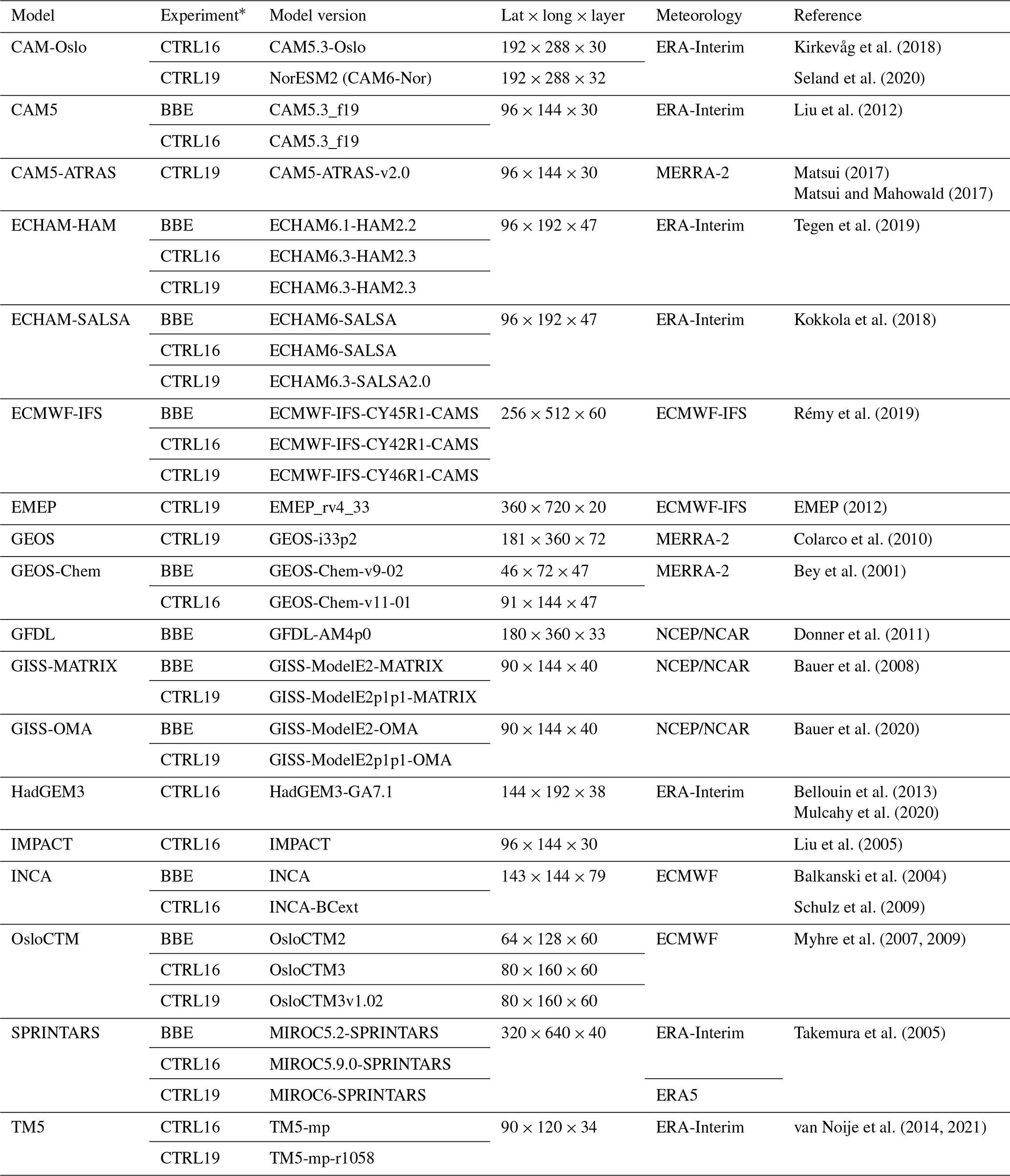
∗ Models participated in one or multiple experiments with either
the same or different model versions. The experiments include biomass
burning emissions (BBE) for 2008;
control 2016 (CTRL16) for 2006, 2008, and 2010; and
control 2019 (CTRL19) for 2010.
2.1 Models and variables
This study evaluated the AOD at 550 nm simulated by models from three AeroCom Phase-III experiments: the biomass burning emissions experiment (BBE), control experiment 2016 (CTRL16), and control experiment 2019 (CTRL19). A total of 18 different models were investigated in our study, with parts of the models participating in multiple experiments with different versions. Table 1 provides an overview of these models; more details are provided in the Supplement and listed references. The general settings of the three experiments were as follows.
The aim of BBE was to quantify the impact of BBA emissions on AOD simulations. All the participating models presented simulations for the year 2008 using the prescribed BB emission input (GFED3). In addition, simulations with scaling factors of 0, 0.5, 2, and 5 (referred to as BBE0, BBE0.5, BBE2, BBE5) adapted to GFED3 emissions were also provided. These scaling factors were based on a preliminary simulation by the Goddard Chemistry Aerosol Radiation and Transport (GOCART) aerosol model, which found that using default GFED3 emissions would lead to AOD underestimations over most fire regions (Petrenko et al., 2012). The perturbations in emissions would allow a quantitative analysis of the AOD emission response.
The models in CTRL16 adopted the standard diagnostics and presented simulations for 2006, 2008, and 2010. The modelers were advised to nudge the meteorology to (or drive the models by) their preferred datasets (see Table 1). The standard outputs mainly included 2-D fields at a monthly frequency, which were extended by several other experiments launched subsequently (e.g., the remote sensing experiment). High-frequency (3 h) AOD data together with other information (e.g., 3-D fields of the AOD) are currently available. In this study, we examined 12 models with an AOD output at a 3 h frequency for 2006, 2008, and 2010.
The state of the art of aerosol modeling for 1850 (pre-industrial era) and 2010 (present day) was assembled in CTRL19. All models were nudged to (or driven by) a fixed sea surface temperature and 2010 meteorology using different data sources (see Table 1). Emissions from the Coupled Model Intercomparison Project Phase 6 (CMIP6) were used when applicable. The model AOD was output at a daily or monthly frequency. In this study, we selected 12 models that provided a daily output for 2010.
In addition to AOD, other variables from the models were used to interpret model diversity when available. These additional variables included emissions, total deposition (both dry and wet deposition), aerosol column load (with aerosol species resolved), the vertical profile of the extinction coefficient (EC), precipitation, and the Ångström exponent (AE, which was calculated using the AOD at 440 and 550 nm; the AE-based interpolation was adopted if AOD at 440 nm was not available for some models).
We also prepared a questionnaire filled out by modelers to acquire information on the model configuration details (see Supplement). Information was collected for models in CTRL16 and CTRL19.

Figure 1Three focused fire regions in this study. (a) Global map of BB OC emissions averaged for 2006, 2008, and 2010 based on GFED4.1s (https://www.globalfiredata.org/, last access: October 2021). The domains of the three fire regions are shown by the red boxes together with the AERONET sites (purple dots). (b) The monthly evolutions of BB OC emissions from six fire types in AMAZ (b1), SHAF (b2), and BONA (b3), respectively. The un-collocated regional mean AOD observations from 14 satellite datasets are shown by the light-red-shaded areas as interquartile ranges (only the grid boxes with more than 20 data available in a month are included). Emissions for BB were considered in terms of the biome/fire type: tropical forest and deforestation (DEFO), savanna (SAVA), temperate forest (TEMF), boreal forest (BORF), peat (PEAT), and agricultural waste (AGRI).
2.2 Fire regions
Based on the models considered, three key BB regions were selected in this study: the Amazon (AMAZ), Southern Hemisphere Africa (SHAF), and boreal North America (BONA). Figure 1 shows the domains of these three regions and the corresponding OC emissions from BB. In terms of their aerosol emission, different fire types could be identified in each region. The BB emissions in AMAZ were dominated by tropical forest fires and deforestation, whereas emission from savanna grassland fires was the major source in SHAF. In BONA, BB aerosols were mainly emitted from boreal forest fires. Regions with agricultural waste burning or temperate forest fires were not considered due to their small contribution on a global scale (van der Werf et al., 2010). Using the satellite observation of AOD, we defined the fire seasons (dry seasons) over the three regions (see Fig. 1b) that were investigated in this study.
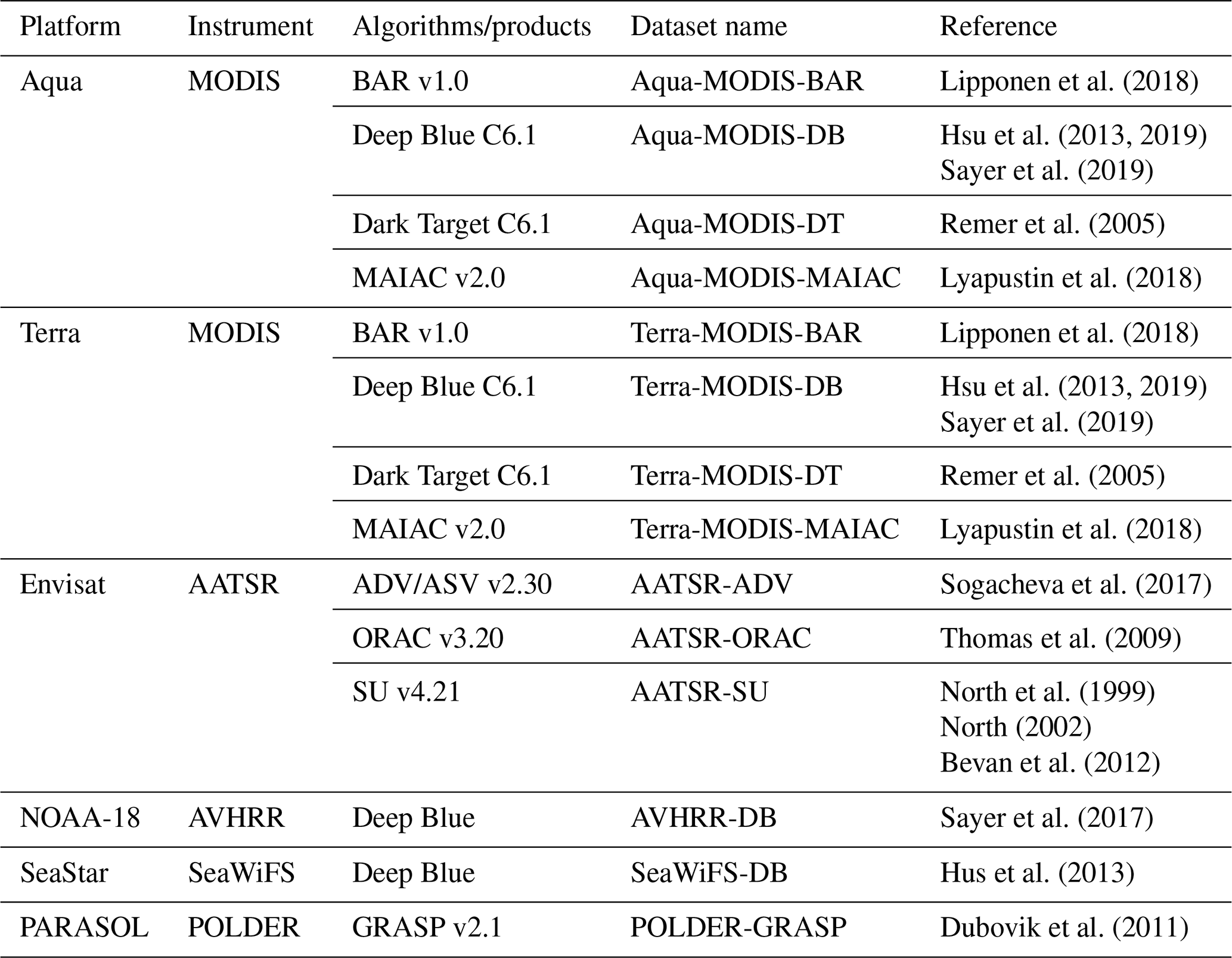
2.3 Observation data
A total of 14 satellite AOD datasets were used in this study. Table 2 provides an overview of the datasets. The AOD data at 550 nm wavelength were obtained by either direct retrieval or interpolation/extrapolation from the AOD at nearby wavelengths.
The ground-based remote sensing data were taken from AERONET DirectSun L2 v3 (Dubovik et al., 2000). The locations of the AERONET sites within the three fire regions are shown in Fig. 1a. Given that the sparse distribution of AERONET sites results in poor spatial data coverage, especially in SHAF and BONA, we mainly used the AERONET data to evaluate the satellite datasets, while model validations relied on satellite data.
For the vertical profiles, we used the Cloud-Aerosol LIdar with Orthogonal Polarization (CALIOP) L2 layer 5 km v4.20 product. The EC data at 532 nm were compared with models (at 550 nm) where the vertical data were available. For CALIOP data, we only considered columns that had at least one aerosol retrieval based on the cloud–aerosol discrimination (CAD) scores (CAD ) (Watson-Parris et al., 2018). Columns with extreme CAD scores () were also excluded because they might have been the result of bad shots (Watson-Parris et al., 2018). To ensure data quality, we only used the most reliable retrievals that had extinction quality control (QC) flags of 0, 1, 2, 16, or 18. In addition to the direct comparison of vertical extinction profiles, we calculated the weighted mean plume extinction height (PEH) based on the vertical EC and layer height (hi) for the aerosol layers below 6 km (Koffi et al., 2016), as shown by Eq. (1):
In addition, we evaluated the modeled precipitation as it is the cause of a major deposition process. The precipitation data were taken from the Global Precipitation Climatology Project (GPCP), which incorporates precipitation from low-orbit satellite data, geosynchronous satellite data, and surface raindrop observations (Adler et al., 2003).
2.4 Data analysis
To mitigate sampling issues associated with sparsely distributed observations, we conducted strict collocations before the data were evaluated (Schutgens et al., 2016a, b). Both model and observation data were firstly re-gridded into the spatial grid boxes. The temporal resolution was aggregated into 3 h or daily intervals according to the model output frequency (see Table 1). For the satellite validation against AERONET, we compared satellite data with AERONET at the resolution of h. Especially the plume height in models was validated against CALIOP on a monthly basis since CTRL19 models only provided data at such a resolution. Vertically, the CALIOP data were aggregated into 100 m intervals, and all the extinction profiles from models were linearly interpolated into the same resolution for validation.
The data aggregation and collocation were processed via a command-line tool called Community Intercomparison Suite (CIS; Watson-Parris et al., 2016). To quantitatively evaluate the model performance and satellite observation uncertainties, we utilized Taylor diagrams to present the statistics, including the Pearson correlation coefficient (r), standard deviation (SD), and centered root mean square error (CRMSE) (Taylor, 2001). Taylor diagrams are presented in polar coordinates with the polar axis showing the SD of evaluated data and cosine of the polar angle showing the r value between evaluated and “reference” data. The distance between the evaluated and reference data shows the CRMSE according to the law of cosines. Both evaluated and reference data were normalized by the SD of reference data so that the reference was always located at [1, 0] (see Fig. 2a for an example). A Taylor diagram is a convenient way to visualize the performance of models or observations versus a reference dataset. However, bias is not shown by Taylor diagrams, and we accompanied each Taylor diagram with a plot showing the normalized mean bias (NMB, defined as the mean bias divided by the mean value of observation) to provide a comprehensive evaluation.

Figure 2Comparison of the 14 satellite AOD products against AERONET observations as shown by a Taylor diagram (a) and scatter diagram of NMB (b). The colors and shapes of dots indicate different satellite datasets and fire regions. All the satellite data were individually collocated with AERONET data during the fire seasons. POLDER-GRASP and SeaWiFS products over BONA are not shown because the available sample size was too small (<5) after collocation.
3.1 Validating satellite products against AERONET dataset
A large number of satellite AOD datasets have become available, and it is important to use the dataset that can adequately serve the specific research goal. In light of the uncertainties in satellite observations, we evaluated individual satellite datasets against AERONET observations before model validation in the three fire regions. The evaluation was only conducted for data during the fire seasons, and most observations were collected over AMAZ.
Figure 2 shows the evaluation of 14 satellite datasets against AERONET observations for the three fire regions during the fire season. The data points in the Taylor diagram were normalized by AERONET data with different sampling for each product (Fig. 2a), while NMBs are shown in the scatter diagram (Fig. 2b). All the satellite datasets agreed with AERONET observations over AMAZ better than the other two regions, with stronger correlations (r=0.85 to 0.95) and lower normalized CRMSE (<0.5). For AMAZ, all the datasets had similar correlations and CRMSEs but very different biases. The Polarization and Directionality of the Earth’s Reflectances measurements with the Generalized Retrieval of Aerosol and Surface Properties algorithm (POLDER-GRASP) dataset and two algorithms adopted to Moderate Resolution Imaging Spectroradiometer (MODIS) data (BAR and Dark Target) tended to overestimate AOD (3 % to 13 %), while the others resulted in underestimations (−1 % to −20 %). Unlike in AMAZ, individual satellite products agreed less well with AERONET and there were strong variations within each of them over SHAF and BONA (r=0.31 to 0.91, CRMSE = 0.51 to 1.71). All products except Aqua-MODIS-BAR underestimated AOD over SHAF (−7 % to −73 %), whereas most products overestimated AOD over BONA by up to +73 %. Both the spatial data coverage and the temporal data coverage in BONA and SHAF were much lower than in AMAZ, probably due to the higher surface reflectance (less forested), which made the retrievals more difficult and less accurate (Fraser and Kaufman, 1985). Generally, we found that MODIS products agreed well with the AERONET data, although details vary by the retrieval algorithm. For example, the MODIS-BAR products were the best in AMAZ and SHAF, while the MODIS-MAIAC product was better than the others in BONA. From the perspective of bias, we found that the variations among satellite products were affected more by the algorithm than the instrument, which was related to the amount of spectral information used in the retrieval. For example, the data spread of the four instruments that adopted the DeepBlue algorithm (i.e., Aqua-MODIS-DB, Terra-MODIS-DB, AVHRR-DB, and SeaWiFS-DB) was smaller than that for the MODIS products that used four different algorithms (i.e., BAR, DB, DT, and MAIAC) for all three regions.
It should be noted that the evaluation was affected by representation issues. As shown by Fig. 1, there were more AERONET sites located in fire areas in AMAZ, while in SHAF, the AERONET sites were far from the fire emission sites and the downwind area and only captured a small part of the BB aerosol signals. In BONA, the temporal coverage of both AERONET and satellites was poor. Due to the stratocumulus and low broken cumulus cloud contamination, satellite retrievals of AOD were enhanced, which could lead to unexpected overestimations when compared with the ground-based observations over BONA (Toth et al., 2013).
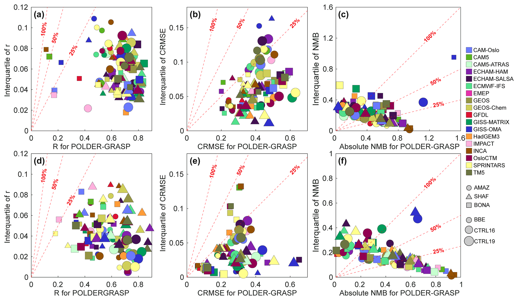
Figure 3Variation in model AOD evaluation due to different choices of satellite products in terms of the correlation coefficient (a, d), centered root mean square error (b, e), and normalized mean bias (c, f). The results are shown as comparisons between the values using POLDER-GRASP (horizontal axis) and interquartile ranges (vertical axis) when validating each model with different satellite products. The top (a–c) and bottom (d–f) panels show the results for individual and synchronous collocation, respectively. The color, shape, and size of dots indicate different models, three fire regions, and three AeroCom experiments, respectively. The dashed lines show the 25 %, 50 %, and 100 % slopes (the interquartile relative to POLDER-GRASP). The GISS-OMA data for BBE over BONA are not shown in (b) due to the very high CRMSE.
3.2 Impacts of different satellite datasets on model validations
In this study, we utilized POLDER-GRASP to evaluate all the models. AOD from POLDER-GRASP has been validated in a previous study which suggests POLDER-GRASP is superior to other products globally (Schutgens et al., 2021). The AE data have also been validated before, showing a good agreement with AERONET (Chen et al., 2020). In our study, we also investigated how the observation uncertainties mentioned above may affect model validations, which were indicated by the interquartile ranges of the r, CRMSE, and NMB based on validations using different satellite products. The interquartile values were further compared with the statistics (i.e., r, CRMSE, and NMB) when using POLDER-GRASP to show the uncertainty range when using the specific dataset. Before calculating the difference in model validation (i.e., r, CRMSE, NMB) due to different satellite products, each model was collocated with satellite products either individually (i.e., all the models were collocated with the different sampling of each satellite product; see Fig. 3a–c) or synchronously (i.e., the model data were collocated with the same sampling where all satellite products could provide data; see Fig. 3d–f). In the latter case, only products that had a similar overpass time to POLDER-GRASP were considered (i.e., with an overpass time in the afternoon, excluding datasets on board Terra and Envisat). For comparison, the uncertainty ranges of 25 %, 50 %, and 100 % for the interquartile for the spread of multiple products relative to POLDER-GRASP are also shown.
For the individual collocation case, we found that the uncertainties in r and CRMSE (Fig. 3a–c) due to the different satellite products were generally lower than 25 %, indicating a small impact when using different satellite datasets. The impact on CRMSE was slightly stronger than that on r, which suggested that different satellite products tended to have higher consistency in capturing the spatiotemporal variations than the magnitude of AOD. In the case of NMB, the impacts of verifying against different satellite data products were large only when the modeled NMB was small (<20 %). The majority of simulations had an NMB higher than ±40 %, suggesting the uncertainties among the different satellite products were less important for NMB and the modeled bias was dominated by the biases in the model instead of the difference in satellite products.
For the synchronous collocation which eliminated the sampling differences (Fig. 3d–f), similar results were obtained with even much smaller satellite uncertainties. In this case, all the satellite products were collocated, which greatly reduced the frequency of cloud contamination issues and provided more reliable results. Due to the synchronous collocation, a large portion of the original observations was filtered and statistical noise may stand out. We then conducted a 10 000-time bootstrap sampling with replacement to examine the potential effects of such noise. Each time, we randomly excluded 20 % of the data to test the robustness of our evaluations. The coefficient of variation for the satellite observation uncertainties from the 10 000-time bootstrap sampling was 1 % to 10 % for r, 1 % to 12 % for CRMSE, and 3 % to 27 % for NMB. For the stronger variation in NMB, over 85 % of simulations were subject to an NMB variation of less than 10 %, suggesting very robust results for the above analysis. All this indicated that although there were different errors in these satellite products, only a small part (accounting for <25 % of the modeled errors) could be expected to affect the model validation. Given the small impacts, we decided to validate models against the POLDER-GRASP product for both AOD and the AE, which provided a degree of consistency for the whole analysis.
Though model validations during fire seasons would not be altered much by using different satellite datasets, this is not the case for other areas/periods. For example, in the same fire regions outside the fire seasons, we found that the uncertainties due to different satellite products could be as high as 50 % in most cases (not shown). Therefore, we highly recommend evaluations of satellite datasets before using them for model validations.

Figure 4Validation of AeroCom models against POLDER-GRASP observations for AOD during fire seasons. The validations of models from the three AeroCom experiments are shown as Taylor diagrams for BBE (a), CTRL16 (b), and CTRL19 (c). The NMB for all the models is shown in panel (d). The colors and shapes of dots indicate different models and fire regions. All the model data are collocated with POLDER-GRASP data. The evaluation is for 2008 in BBE; for 2006, 2008, and 2010 in CTRL16; and for 2010 in CTRL19. The GISS-OMA data for BBE over BONA are not shown in (a) due to the very large normalized CRMSE.
We then evaluated AOD in AeroCom models in three experiments using the POLDER-GRASP product. All model data were collocated with POLDER-GRASP sampling. The model evaluation is shown in Fig. 4 via Taylor diagrams and bias plots. The r values ranged from 0.1 (INCA over BONA in BBE) to 0.78 (ECMWF-IFS over SHAF in CTRL19) for all models and regions, with a median value of 0.63. Over 80 % of the model simulations had an r value higher than 0.5, but only 24 % of simulations had correlations stronger than 0.70, suggesting a generally moderate capability for capturing the spatiotemporal variation in aerosol data. For CRMSE, the modeled variation (defined as the interquartile range divided by the median value, 51 %) was stronger than that for r (22 %), indicating a higher modeled disparity of the AOD magnitude than the spatiotemporal trends. Based on an analysis of variance for r and CRMSE (Fig. 4a–c), we found that the models showed similar performance over the three regions as there was no significant difference found. The median NMBs of models (Fig. 4d) for AMAZ, SHAF, and BONA were −28 % (−6 % to −54 % as interquartile), −54 % (−30 % to −63 %), and −54 % (−46 % to −57 %), respectively. Models produced significantly smaller NMB over AMAZ than over the other two regions, though the inter-model variation was also found to be the highest among the three regions. More than half of the simulations showed an underestimation of AOD by a factor of >2, consistent with previous studies (e.g., Kaiser et al., 2012; Veira et al., 2015; Johnson et al., 2016). In Fig. 5, we compared the daily AOD series for the model ensembles with POLDER-GRASP observations. For most models, the underestimations of AOD tended to be exacerbated during the peak of observations.
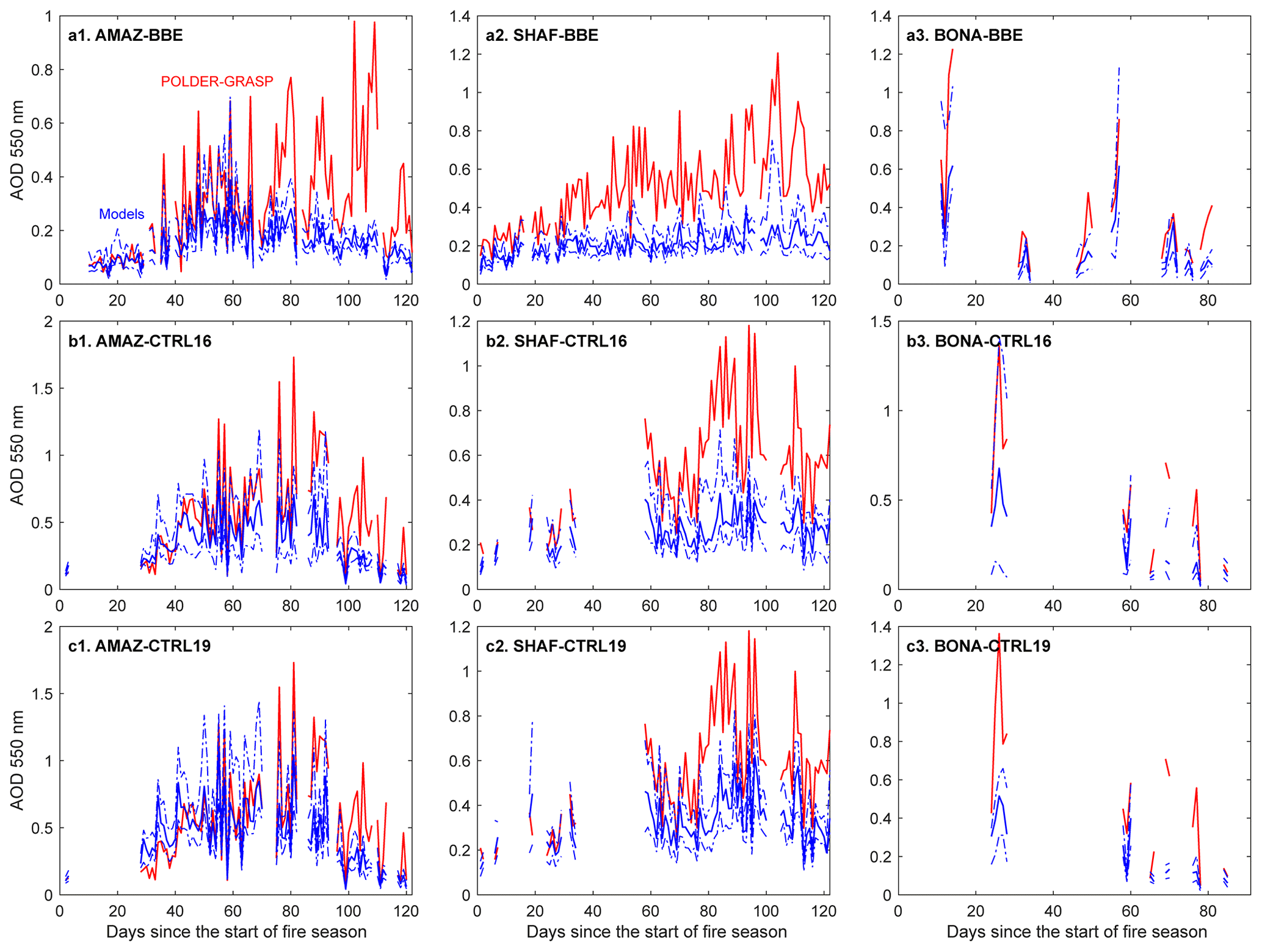
Figure 5Daily time series for the AOD mean bias for AMAZ (a1–c1), SHAF (a2–c2), and BONA (a3–c3) in BBE (a), CTRL16 (b), and CTRL19 (c) experiments. All the model data are collocated with POLDER-GRASP during fire seasons. Data are shown for 2008 for BBE and 2010 for CTRL16 and CTRL19.
In addition to the overall model evaluations, we also evaluated the modeled temporal (time series for all the fire regions) and spatial patterns (temporal averages for individual grid boxes during fire seasons). In Fig. 6, we compared the temporal and spatial correlations of modeled AOD with observations. Most models showed similar temporal and spatial correlations ranging from 0.6 to 0.9, which were slightly higher than the overall correlations shown in Fig. 4 due to data averaging. Both the spatial and the temporal correlations in most models clustered in this range, which partly explained the similarity of the overall correlations mentioned above. We found there was no significant difference between the temporal and spatial correlations in individual models from the three experiments. Although the AOD errors differed substantially per model, the spatial and temporal variation among models tended to be small. For the model ensembles, we found there was no significant difference among the three experiments for both spatial and temporal correlations, even though improvements might occur in emission inventories and/or models following the time sequence from BBE to CTRL16 to CTRL19. We also compared the variations in temporal and spatial AOD biases, as shown in Fig. 7. Here the variations were defined as the ratio of interquartile to median values of the time series (temporal variations) or spatial averages (spatial variations) of absolute modeled AOD bias. The spatial variations were significantly smaller than temporal variations for all three experiments, suggesting the different temporal evolution of AOD biases was the leading cause of the large NMB diversity in Fig. 4. It partly suggested that current emission inventories had a better representation of BBA emissions over space than over time.
Since the modeled AOD bias is strongly affected by input emissions (Kaiser et al., 2012; Johnson et al., 2016), we also investigated the model response to the changes in emissions based on BBE. This scaling-up procedure has been used to fix overall AOD errors for BBA in previous studies (e.g., Kaiser et al., 2012; Johnson et al., 2016; Veira et al., 2015). Figure 8 shows the evaluation of these models for r, CRMSE, and NMB. As expected, NMB increased monotonously with the increase in emissions. Most models would produce significant positive bias when the scaling factors to GFED3 reach 5, but more than half of models still underestimated AOD when BBA emissions were doubled. Such trends were also found for CRMSE with a much weaker sensitivity. Similar phenomena were also found in the other two experiments. For example, we found the ECHAM-HAM model agreed well with observation in the CTRL16 experiment which used 3.4 × GFAS emissions, while it produced large underestimation when the CMIP6 emissions (much lower than 3.4 × GFAS) were used (see Fig. 4d). Given the metrics of CRMSE and NMB, the ensemble of models in BBE showed the best agreement with observations when the emissions were scaled by a factor of 2. This systematic response of modeled bias also suggested a possible underestimation of emissions in the applied inventory (GFED3). However, correlations in most models did not improve along with the increased emissions since there was no further spatiotemporal information added into the emissions.
The modeled AOD bias during fire seasons could be due to both BBA and background sources (e.g., anthropogenic, biogenic, dust, and sea salt aerosols). However, it is difficult to isolate BBA errors from the background based on existing simulations. Since we found that most models underestimated AOD in the BBE1 simulations, it was not possible to determine the real BBA impacts by comparing BBE1 and BBE0 simulations. Instead, we compared the collocated BBE0 AOD (background) with POLDER-GRASP observation during fire seasons. The modeled AOD in BBE0 varied substantially by a factor of 9 in the three regions. Compared with observations, the background averagely accounted for only 14 %, 12 %, and 11 % of total AOD over AMAZ, SHAF, and BONA, respectively. We also compared the modeled AOD biases during non-fire seasons with those during fire seasons, with the former showing much smaller magnitude compared with the latter (0.04 vs. 0.35, for the absolute mean bias). This analysis supports the notion that AOD bias over the fire regions was dominated by the BBA rather than background sources.
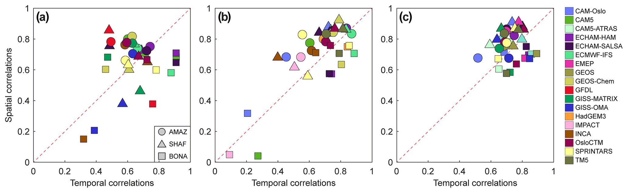
Figure 6Comparison of the temporal and spatial correlations between modeled AOD and POLDER-GRASP observations. Results are shown for the three experiments individually (a BBE, b CTRL16, c CTRL19). All the model data are collocated with POLDER-GRASP during fire seasons. The correlations are then calculated using either the time series of the regional averages (horizontal axis) or the spatial averages for all the fire seasons (vertical axis). The dashed red lines show the 1:1 range.
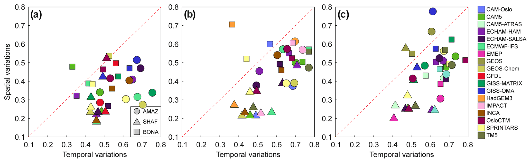
Figure 7Comparison of the temporal and spatial variations in modeled AOD errors. Results are shown for the three experiments individually (a BBE, b CTRL16, c CTRL19). All the model data were collocated with POLDER-GRASP. The variation is calculated as the ratio of interquartile to median values of the absolute bias for time series (temporal variations) and spatial averages (spatial variations). The dashed red lines show the 1:1 range.
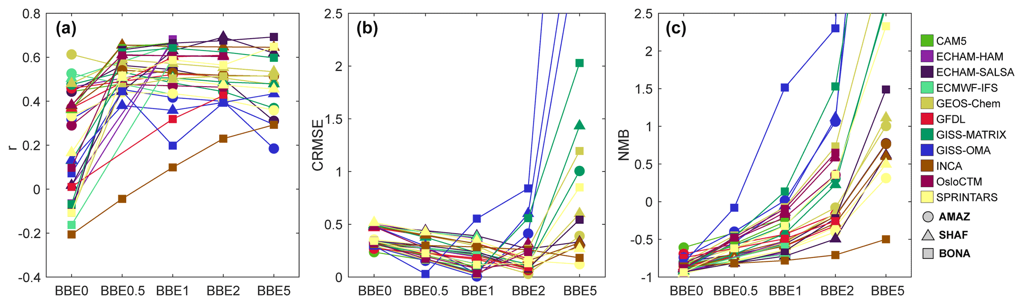
Figure 8Changes in correlation (a), centered root mean square error (b), and normalized mean bias (c) in BBE in responding to different scaling factors adopted to BBA emissions (0, 0.5, 2, 5). The colors and shapes of dots indicate different models and fire regions. All data are collocated with POLDER-GRASP for fire seasons in 2008. The BBE5 CRMSE and NMB for several models are not shown given the extremely large values.
As the above model evaluation could not provide sufficient information on the causes of the model biases, we explore the diversities of AOD in this section. Our strategy is to first evaluate the diversity in modeled AOD and the possible drivers that could lead to such variability and then compare those drivers with available observations to understand the model variability and therefore bias. This practice will also contribute to future model development. Unless stated otherwise, data in this section are presented as area averages for the whole fire season based on the raw model outputs without any collocation. The aim is to determine the general drivers of variation in AOD for model ensembles rather than individual models, although evaluations for specific models are also presented where sufficient information is available.
5.1 Decomposition of modeled AOD diversity
The diversities of AOD were decomposed into three factors, i.e., total aerosol emissions, aerosol lifetime, and the MEC, as described by the following function:
where emission indicates the total emissions of OA (including secondary organic aerosols, which were treated as emitted aerosols given the fast transformation), BC, sulfur dioxide (SO2), sulfate (SU), mineral dust (DU), and sea salt (SS) within the fire regions; lifetime is defined as the average total aerosol load divided by total emissions within the fire regions; and the MEC is defined as AOD divided by total aerosol load, which is strongly associated with the modeled aerosol optical properties (e.g., size distribution, refractive index, hygroscopicity). Emissions, aerosol load, and AOD were first calculated as regional and seasonal averages so that the lifetime and MEC were determined on a seasonal level for the focused regions. Note that the definition of lifetime in this study is different from the usual one as we are considering open systems. However, the timescale here called lifetime is still determined by the same relevant process (e.g., deposition). This is discussed in detail in Sect. 5.1.
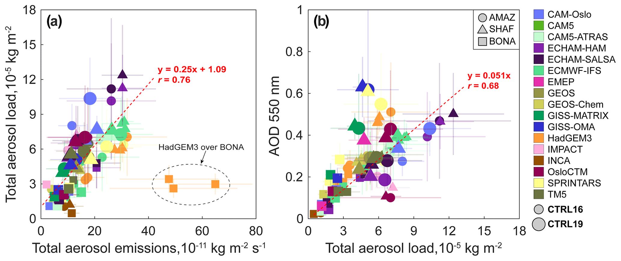
Figure 9The dependence of total aerosol load on total aerosol emissions (a) and dependence of AOD on aerosol load (b), indicating the aerosol lifetime and MECs, respectively. The data are average values for all the fire seasons based on the raw model output without collocation, and the light-colored error bars indicate the corresponding temporal variations (as standard deviation). The color, shape, and size of dots indicate different models, three fire regions, and two AeroCom control experiments, respectively. The dashed red lines show the linear trends, with a regression function and correlation coefficients (r) also shown. Note that some CTRL16 models provide data for different years (2006, 2008, and 2010), which are illustrated separately.
Figure 9 shows the diversities of the three factors. The slope of the line between each dot and the origin indicates the aerosol lifetime (Fig. 9a) and MEC (Fig. 9b) for a specific model averaged for the whole fire season, respectively. The emissions varied by a factor of 10 among the models. Such large deviations resulted from different emission inventories (mainly for CTRL16 models) and the different schemes for estimating non-BB aerosols (e.g., dust, biogenic sources). For the CTRL19 experiment with its prescribed emission inventory (CMIP6), the input emissions were altered mainly by the different ratios and to a lesser extent by the different mechanisms of DU production and biogenic sources. For example, the ratios were set as 1.4, 1.8, and 2.6 in ECHAM-HAM, GEOS, and SPRINTARS, leading to emissions being 34 % and 88 % higher in the latter two models, respectively. The difference in these ratios is a consequence of the different assumptions regarding the oxidation of freshly emitted OC. The widely used ratio of 1.4 was established based on field measurements over urban regions (Turpin and Lim, 2001) and was therefore more representative of anthropogenic OC emissions. More recent investigations of the BB plume have suggested that the oxidation levels are higher for both fresh and aged BB OC particles (Aiken et al., 2008; Brito et al., 2014; Tiitta et al., 2014). Increasing the ratio can directly lead to an elevated AOD in models, and a ratio higher than 1.4 has been suggested for BB aerosols in some previous studies (e.g., Reid et al., 2005; Aiken et al., 2008; Johnson et al., 2016). Omitting GISS-MATRIX and GISS-OMA which produced an unexpected positive AOD bias (see Fig. 4), we found that the modeled NMB generally decreased with an increase in the ratio for CTRL19 models. For example, the average NMB of AOD for the model group that used the ratio of 1.4 (i.e., CAM5-ATRAS, ECHAM-HAM, and ECHAM-SALSA) was −61 %, whereas the value was only −22 % for the group using a ratio of 2.6 (i.e., CAM-Oslo, NorESM2, OsloCTM, and SPRINTARS). The NMB of the models using a ratio of 1.6 to 1.8 was within an intermediate range (−43 % to −46 %). This shows the importance of determining realistic values of the ratio. However, it does not necessarily mean that higher ratios can address the underestimated AOD. For example, both SPRINTARS and OsloCTM produced significant overestimations in AMAZ using an ratio of 2.6 that was higher than many in situ observations (e.g., Brito et al., 2014; Zheng et al., 2017).
When all three fire regions were considered simultaneously, there was a general linear response of the aerosol load to aerosol emissions and of AOD to aerosol loads. Nevertheless, significant diversities in the lifetime and MEC were found. For the three regions, the relative variation (i.e., interquartile value divided by the median value) was found to be the lowest for the MEC (49 %, 41 %, and 40 % for AMAZ, SHAF, and BONA, respectively), moderate for aerosol lifetime (62 %, 49 %, and 26 %, respectively), and highest for emissions (62 %, 95 %, and 64 %, respectively). For the aerosol lifetime and MEC, which were mainly affected by model aspects other than emissions, we found their ensemble median values were similar among the three fire regions. HadGEM3 over BONA presents an outlier case for lifetime, which is probably related to high local DU emissions. We also noticed that the DU emission in HadGEM3 covered a much wider area than in the other models due to the use of different mechanisms (Woodward, 2001; Mulcahy et al., 2020).
The contributions of aerosol emissions, aerosol lifetime, and the MEC (which were found to be statistically independent of each other) to the overall variation in AOD were evaluated. We used Eq. (2) to investigate such contributions. In the case of the AOD variation induced by emissions, we calculated the AOD variation (i.e., the standard deviation) over all modeled emissions and a random combination of aerosol lifetime and MEC values from the model ensemble. This calculation was repeated for all the combinations of aerosol lifetime and the MEC, and the variation in AOD attributable to emissions was then quantified as the average value of all the standard deviations. Similar calculations were also applied to aerosol lifetime and MEC values. It was estimated that aerosol emissions, aerosol lifetime, and the MEC accounted for 38 %, 33 %, and 29 % of the variation in AOD, respectively, suggesting only small differences in determining the overall variation, although emissions might be slightly more important than aerosol lifetime and the MEC. We also applied this evaluation to individual fire regions, and similar conclusions were obtained. This suggests that reducing the uncertainties associated with emissions uncertainties might have only a moderate impact on the accuracy of the BBA simulations, and uncertainties in the lifetime and MEC should also be considered.
5.2 Diversity of aerosol lifetime
In this section, we discuss the potential factors that contribute to the diversity of aerosol lifetime. Because we focused on three separate open systems, we described the aerosol budget of each region as a simple box model, as shown by Eq. (3):
where B, E, D, I, O, P, and L indicate the average of total aerosol burden, emission, deposition, inflow, outflow, chemical production, and chemical loss of a focused region. For a closed system and a steady state without chemistry, I and a lifetime can be defined as . For an open system and steady state and with ongoing chemistry, does not equal but both are still timescales defining the system. Here we show that for these fire regions, correlates with . Figure 10 displays the linear dependence of the modeled aerosol lifetime on the timescale of total deposition and all other processes. For most models, the reciprocal of aerosol lifetime ( responded linearly to the timescale of deposition (, except for INCA from CTRL16. This suggests that the difference in deposition is a leading contributor to the variation in aerosol lifetime. HadGEM3 simulations in BONA (the outliers of the aerosol lifetime trend in Fig. 9) still followed the same linear trend, confirming that the short aerosol lifetime is a direct result of the strong deposition of coarse mineral dust. For INCA, the simulated aerosol load was much lower than other models, and the modeled aerosol composition was very different with OA contributing less than 20 % of the total aerosol load. As a result, the coarse-mode aerosols dominated the total aerosol composition, resulting in a relatively short aerosol lifetime. When the INCA model was omitted, the correlation between the reciprocal of aerosol lifetime and the deposition timescale (i.e., deposition load) was 0.95, suggesting that 90 % of the modeled variation in aerosol lifetime could be explained by deposition. The variation in regional transport and the chemical budget together only contributed around 10 % of the variation in aerosol lifetime and was therefore much less important to the overall difference in AOD. The timescale of the total deposition had a variation of 72 % (i.e., the interquartile value divided by the median), which was slightly higher than the aerosol lifetime (62 %).
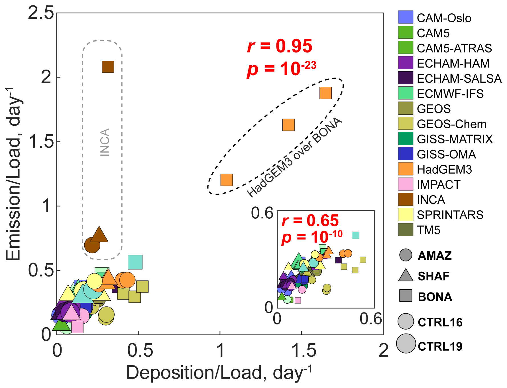
Figure 10Dependence of the modeled aerosol lifetime on the timescale of total deposition. The color, shape, and size of dots indicate different models, three fire regions, and two AeroCom control experiments, respectively. The embedded diagram shows the same results zoomed in to a smaller scale (excluding INCA and HadGEM3 in BONA). The Pearson correlation (r) and p value (p) are shown.
The modeled deposition was primarily a consequence of wet deposition (61 % of the total deposition on average) even during the dry fire season. The modeled wet deposition, which occurred mainly due to below-cloud scavenging (Andronache, 2003; Zhang et al., 2004), was related to the size distribution of aerosols and raindrops as well as to the precipitation intensity (Seinfeld and Pandis, 2006). Figure 11 compares the modeled timescale of total deposition and precipitation strength. Note that not all models provided both deposition and precipitation outputs; the conclusion of the evaluation may need to be re-examined when more data become available in the future. The modeled precipitation differed among the models by factors of 3.8, 13.6, and 2.2 for AMAZ, SHAF, and BONA, indicating a substantial model discrepancy. When all regions were considered, there is a significant positive correlation between the modeled precipitation and the timescale of total deposition. For comparison, we also compared models with GPCP data. GEOS, SPRINTARS, and TM5 were among the models with an overestimated precipitation in all three fire regions, which suggested systematic errors in the modeled lifetime. On a regional basis, models exhibited large regional variations. Almost all models tended to overestimate the precipitation over BONA by up to 69 % (ECHAM-HAM from CTRL19), which might partly explain the underestimated AOD in this region. There were large disparities in precipitation simulation over AMAZ, ranging from −21 % to 130 %. In contrast, we found that most models underestimated both AOD and precipitation in SHAF, suggesting other important sources of AOD bias in addition to precipitation. However, we did not observe a clear dependence of AOD biases on precipitation biases. For example, biases of 6 % and −9 % were found for precipitation and AOD, respectively, over AMAZ in CAM5-ATRAS from CTRL19, whereas the corresponding AOD biases were 14 % and −86 % over BONA. This suggests that factors other than precipitation affect AOD biases significantly.
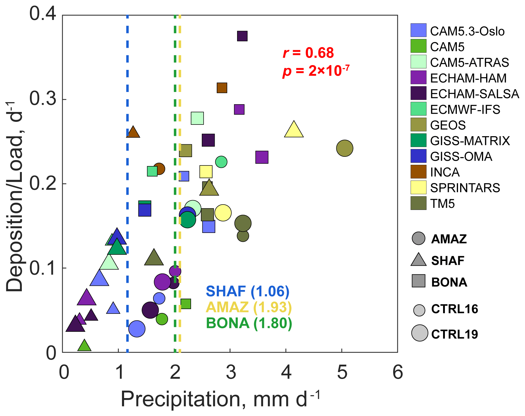
Figure 11Dependence of the modeled timescale of total deposition on precipitation strength during fire season in 2010. The color, shape, and size of dots indicate different models, three fire regions, and two AeroCom control experiments, respectively. The three dashed lines indicate the GPCP data averaged for each region.
In addition to precipitation, we also examined the impacts of aerosol plume height on the aerosol lifetime. Figure 12a compares the modeled plume height (as represented by PEH) and aerosol lifetime. Based on the limited number of models with data available, there was a generally increasing trend in the aerosol lifetime as the plume height increased (r=0.65) except for one outlier (IMPACT over BONA), suggesting that plume height could also affect the modeled aerosol lifetime. Generally, the modeled PEH varied by a factor of 4, partly due to the model assumption in the fire injection height for BB emissions. For example, ECHAM-HAM and ECHAM-SALSA, which allowed 25 % of BB aerosol emissions to be emitted above the planetary boundary layer (PBL), generally had a higher plume height than models that distributed emissions within the PBL (e.g., GEOS, GISS-MATRIX). For validation, we further compared the aerosol vertical profiles between models and CALIOP observations (see Fig. 12b1–b3). To highlight the aerosol layer, we normalized each vertical profile based on the maximum (EC_max) and minimum (EC_min) extinction coefficients to remove the magnitude difference. The normalized EC was calculated as (EC_model − EC_min) (EC_max − EC_min). Over AMAZ and SHAF, only a few models (ECHAM-HAM, ECHAM-SALSA, CAM5-ATRAS, GISS-OMA, and GISS-MATRIX) could capture the peak aerosol extinction at 2 to 4 km, whereas other models tended to show the strongest extinction at lower altitudes or the surface. Over BONA, the observed extinction peaked at ∼4 km, but no models were found with a similar profile. Compared with PEH from CALIOP, the simulated BBA plume tended to be too low for all the models. A similar underestimation was also reported elsewhere for AeroCom models with the bias being attributed to wet deposition being too strong in the models (Koffi et al., 2016).
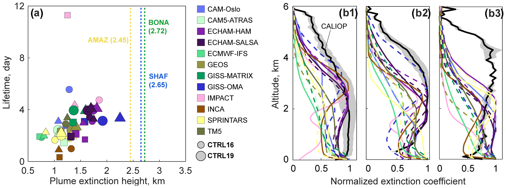
Figure 12Variation in modeled plume height (a) and validation of modeled aerosol vertical profile against CALIOP for AMAZ (b1), SHAF (b2), and BONA (b3). The color scheme in b1–b3 is the same as in (a), with the solid and dashed lines showing the model data from CTRL16 and CTRL19 experiments (if both are available for the same model), respectively. The gray-shaded areas in (b) show the ±σ ranges for the CALIOP observation.
5.3 Diversity of MEC
Modeled MECs are affected by several factors (e.g., particle size, complex refractive index, and hygroscopicity). As BBA is dominated by OA and very similar refractive indices are used in models (see Supplement), the choice of refractive indices is not discussed. Here we mainly examined the impacts of particle size and hygroscopicity.
Because particle size information was missing for the AeroCom models, we used the modeled AE as it is an indicator of particle size (Shuster et al., 2006). Figure 13a shows the dependence of modeled MECs on AEs. The modeled AE varied from 0.21 to 2.2. Ambient particle size is the result of emitted particle sizes and particle processing after emission (see Supplement). Among all models, the lowest AE was found in INCA from CTRL16 due to the large contribution from coarse-mode SS, which also led to lower extinction coefficients because of the lower MECs for SS than OA. When omitting INCA, a significant negative correlation was found between MECs and AEs (), although there were large variations between models. The correlation for CTRL19 models that were driven by the same emission inventory was even stronger (). The negative correlation suggested that a larger size (smaller AE) resulted in a stronger extinction per mass unit for typical BB aerosols, which agreed well with the observations (Laing et al., 2016; Kleinman et al., 2020). This can also be explained by the Mie-scattering theory. In Fig. 13a, we show the relation between MECs and AEs for pure OA based on the Mie-scattering theory. We assumed that the radius of dry OA particles ranged from 0.02 to 0.5 µm. The radius of 0.02 µm corresponded to the smallest emitted particle assumed in all the models examined (see Supplement), and the radius of 0.5 µm indicated the upper edge of the accumulation mode (Tegen et al., 2019). Hygroscopic growth was considered to occur based on the Köhler theory under a relative humidity (RH) of 50 %, and the κ value for OA was set as 0.06 referring to Zhang et al. (2012). A series of sensitive tests suggested that hygroscopic growth did not affect the calculation much. The refractive index was set to 1.53–0.0055i as assumed in most models. The extinction cross-section was retrieved from the lookup table from ECHAM-HAM, based on which MECs and AEs were calculated. The calculated MEC increased with increasing particle size (decreasing AE), which agreed with the modeled relations. Note that many models deviate from our Mie calculation though the Mie theory was applied in those models. Possible causes for such deviations might include, e.g., the aerosol composition (i.e., non-OA components), mixing state for multiple species (e.g., BC), assumptions about the size distribution (e.g., bins, distribution width), and treatment for the mixing of particles with different size distributions.
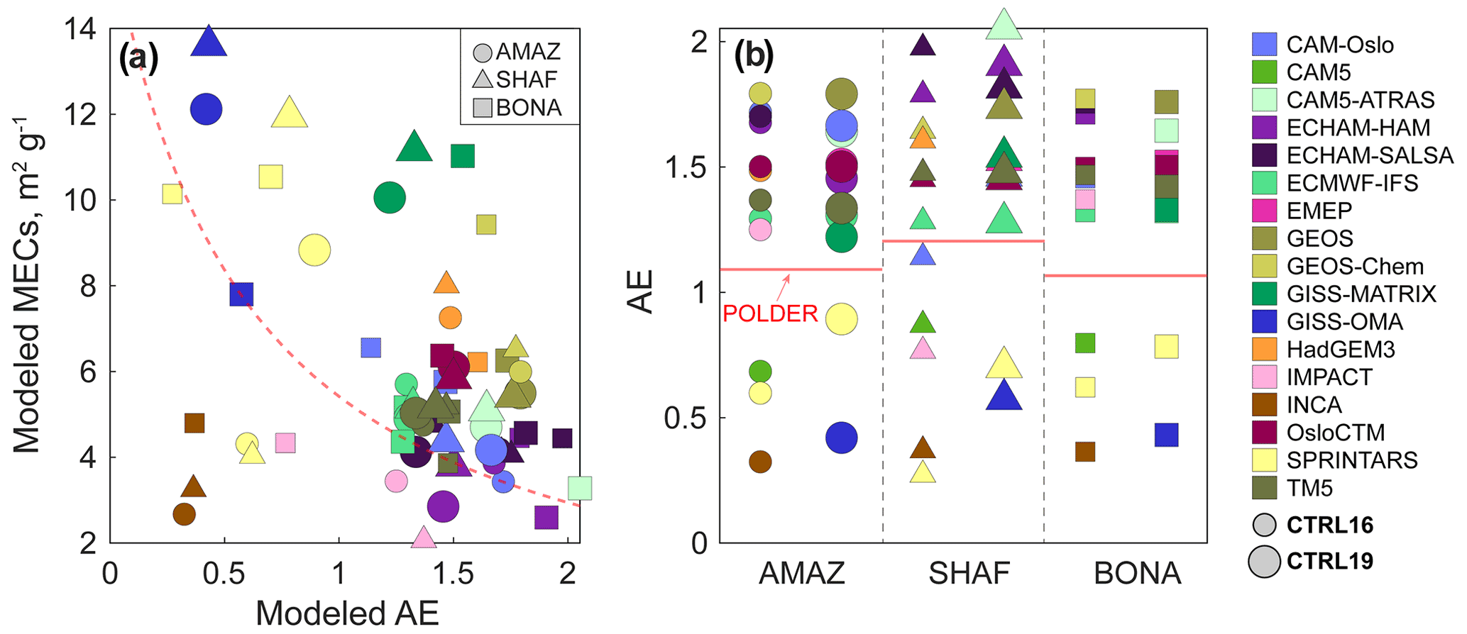
Figure 13Dependence of modeled MECs on the AE (a) and the validation of the modeled AE against POLDER-GRASP data (b). Data in (a) are model original output without collocation. The dashed line in (a) shows the relation calculated based on Mie-scattering theory and the ECHAM-HAM lookup table. Modeled AEs in (b) are collocated with POLDER-GRASP (shown as red lines) on a monthly basis during fire seasons.
The negative correlation between AEs and MECs suggested the possibility of evaluating and subsequently constraining the MEC by the AE. In Fig. 13b we validate modeled AEs against observations from POLDER-GRASP for the fire season. Because most of the AE data for CTRL19 models had a monthly resolution, we collocated all the model data with observations on a monthly basis. Compared with POLDER-GRASP observations, the majority of models tended to overestimate AEs by up to 0.85. BONA had the highest overestimation on average (0.27), followed by AMAZ and SHAF. Given the previous analysis of the MEC dependence on the AE, the underestimation of particle size may have led to a considerable underestimation of MECs and thereby AOD. Similarly to the impacts of precipitation, no strong correlation was found for AOD biases with AE biases, which was largely due to the interaction of multiple factors and a non-linear model response.
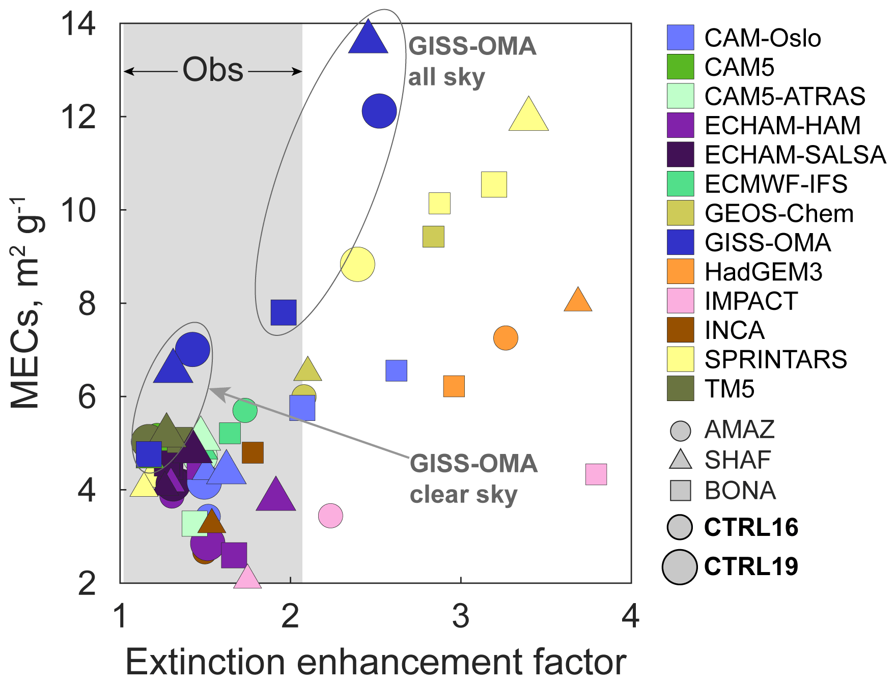
Figure 14Dependence of modeled MECs on extinction enhancement factor (EEF) in models for 2010. The gray-shaded area shows the EEF range from in situ observations according to previous studies (see Table 3). Both clear-sky and all-sky results are shown for GISS-OMA data.
Table 3The extinction enhancement factor (EEF) for BBA at 550 nm wavelength from in situ measurements.
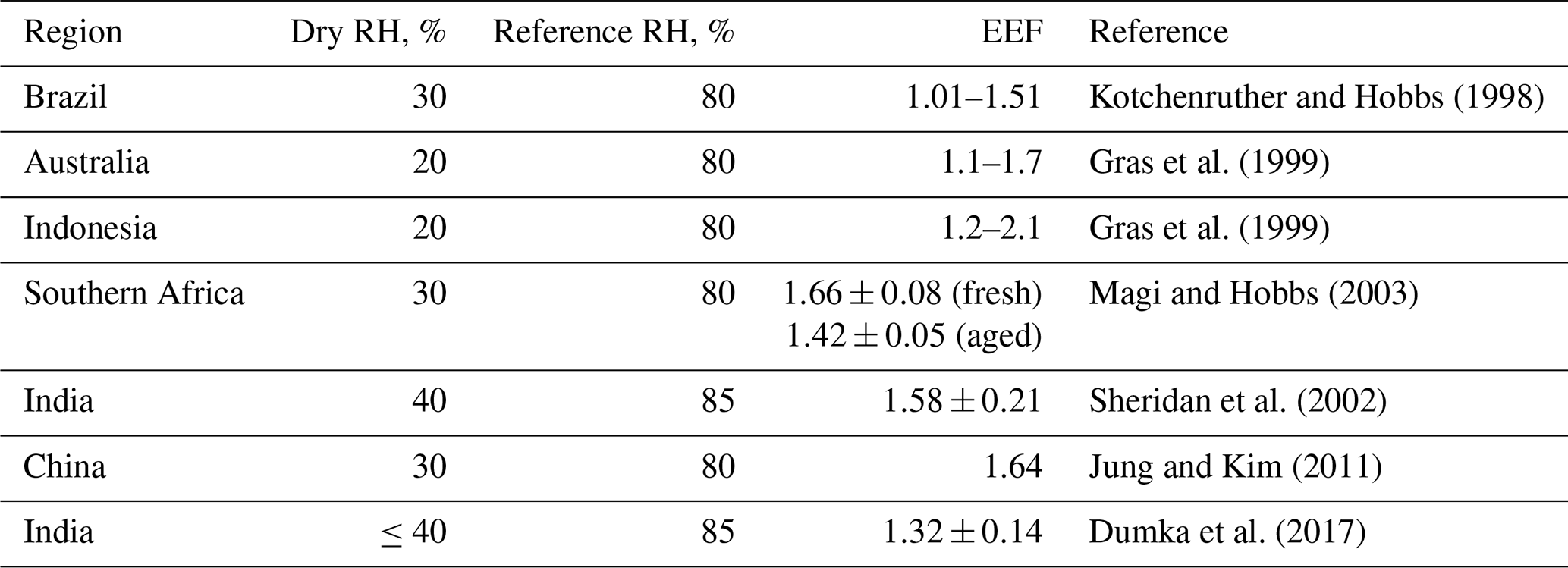
The hygroscopicity was quantified as the extinction enhancement factor (EEF), which was defined as the ratio of AOD at the ambient RH to AOD at zero RH (dry AOD). Figure 14 illustrates the relation between MECs and EEFs in models. For most models, a small EEF (<2) was observed, and we did not observe clear patterns between EEFs and MECs, probably because the hygroscopic growth was not significant given the low hydrophilicity of OA and the dry air conditions during fire seasons. Such a narrow range agreed well with observations from in situ measurements (see Table 3), though the “dry” conditions in measurements (RH = 20 % to 30 %) usually differed from models. Except for these models, there were a few models that showed strong hygroscopic growth, accompanied by a positive correlation with MECs for each model. Such anomalies are related to the assumed BBA properties including, e.g., particle size, mixing state, and hygroscopicity parameterizations for OA given its dominance (Takemura, 2005; Burgos et al., 2020). In addition, we also found the modeled relations between the MEC and EEF were closely related to the treatment of “clear-sky/all-sky” assumptions. For example, the clear-sky data from the GISS-OMA model showed similar EEFs to other models, whereas the all-sky data exhibited much higher EEFs. For those models with higher hygroscopicity (i.e., GEOS-Chem, GISS-OMA, IMPACT, and SPRINTARS), the predicted MECs under the same EEF varied substantially by a factor of 5 per model, suggesting that the modeled MEC diversity was controlled by other factors. When all models were considered together, there was no clear pattern between EEFs and MECs found.
In this paper, we conducted a comprehensive evaluation and interpretation of AOD errors in AeroCom models over three key BB regions. We first evaluated 14 satellite AOD datasets against AERONET and identified their errors. These errors in satellite observations were then compared with model errors, with a much larger magnitude for the latter found in most models. We noticed that such a small impact from different satellite products only applied for our validations over BB regions during fire seasons. Specially, we found that the errors due to different satellite observations were comparable to the model errors for the non-fire seasons over the three BB regions.
Detailed model validations against POLDER-GRASP observations suggested that most of the models still largely underestimated AOD, especially when using the standard emission inventories (e.g., GFED3, CMIP6). We did not observe significant improvements in modeled AOD in the latest experiment (CTRL19) compared with previous ones. The model ensembles from the three AeroCom experiments exhibited a smaller inter-model spread of AOD correlation with observations than AOD errors (e.g., CRMSE, NMB). Models seem to have a similar capability to model the spatiotemporal variation in BBA, probably due to the similarity of input emissions as we found pretty strong correlations (∼0.7) among the emission inventories used by these models (see Supplement). Most of the diversity in model errors is due to a season-wide bias. That said, temporal biases seem larger than spatial biases. We also provided evidence that AOD errors during the fire season were dominated by BBA errors, with only a small contribution from the background. Based on BBE simulations, we found negative biases could be reduced by scaling up BBA emissions. However, we showed that scaling up emissions was not a perfect solution to addressing model bias as the correlations did not improve significantly, suggesting that the spatial and/or temporal bias still existed.
We further analyzed the large diversity in fire AOD as resulting from emissions, lifetimes, and MECs, which all exhibited large diversities too. When all models were considered, we showed that the contributions of these three factors to the overall AOD diversities were similar, though emissions exhibited slightly higher importance. In spite of the large inter-model diversities, the model ensembles show very similar lifetime and MEC values over different BB regions, suggesting that basic model assumptions underlie the lifetime and MEC for the current model ensemble. We suspect that relatively simple changes in these assumptions may produce significant improvement in BBA simulations.
Modeled lifetime was correlated with modeled precipitation strength. Comparisons with observations suggested diverse and region-specific precipitation errors. Modeled lifetime was also related to plume height, which was found to be strongly underestimated by models. We found MECs depended on how models simulate the AE (or particle size). We further compared the modeled AE with POLDER-GRASP observations where general AE overestimations were found in most models. Most models produced acceptable hygroscopicity compared with observations. These findings can provide useful information for future model improvement and development.
There are several uncertainties in our evaluation and analysis. One is the uncertainty in POLDER-GRASP satellite observation. Although we showed that satellite errors did not affect our evaluations very much, we still found that POLDER-GRASP had un-ignorable retrieval errors over the focused regions (13 %). However, the retrieval error was difficult to be precisely defined due to the lack of sufficient sampling in SHAF and BONA by AERONET. On a global scale, POLDER-GRASP was found to be superior to other satellite products used in this study. The other uncertainty stems from the assumption of clear-sky conditions. As we evaluate model AOD against satellite data which are always clear-sky observations, clear-sky model AOD should be used for comparison. However, models have very different treatments of the clear-sky assumption. For example, SPRINTARS considers the 20 % cloud fraction clear sky, while GISS-OMA assumes cloud-free only for 0 % cloudiness. Although strict collocation can partly address this issue, uncertainties may still exist. Such an issue should be investigated more in further model validations.
All the model data can be accessed at the https://aerocom.met.no/ (AeroCom wiki; last access: October 2021). The POLDER-GRASP dataset can be found at https://download.grasp-cloud.com/download/polder/ (GRASP OPEN; last access: October 2021). All the other observations can be found in their references as listed. The data processing in this work was done via CIS (Community Intercomparison Suite; http://www.cistools.net/, last access: October 2021). Codes to create individual figures can be obtained from the corresponding author upon request (q.zhong@vu.nl).
The supplement related to this article is available online at: https://doi.org/10.5194/acp-22-11009-2022-supplement.
QZ and NS proposed the research idea and designed the analysis. QZ carried out the analysis and wrote the paper. NS and GvdW provided scientific advice and valuable suggestions to revise the manuscript. TvN, KT, SEB, TM, AK, ØS, HK, RCG, DN, ZK, HM, PG, TT, PLS, SR, HB, MC, KZ, JZ, SGT, GC, AP, BJ, JEP, NB, RBS, and GM submitted the AeroCom model data used in this study. All the co-authors contributed to reviewing and revising the manuscript.
At least one of the (co-)authors is a member of the editorial board of Atmospheric Chemistry and Physics. The peer-review process was guided by an independent editor, and the authors also have no other competing interests to declare.
Publisher’s note: Copernicus Publications remains neutral with regard to jurisdictional claims in published maps and institutional affiliations.
We acknowledge all the modelers that have submitted AeroCom model data used in this work. Kostas Tsigaridis and Susanne E. Bauer acknowledge NASA MAP for support. Resources supporting this work were provided by the NASA High-End Computing (HEC) Program through the NASA Center for Climate Simulation (NCCS) at Goddard Space Flight Center. Hitoshi Matsui was supported by the Ministry of Education, Culture, Sports, Science and Technology of Japan and the Japan Society for the Promotion of Science (MEXT/JSPS) KAKENHI grant numbers JP19H04253, JP19H05699, JP19KK0265, JP20H00196, and JP20H00638; MEXT Arctic Challenge for Sustainability phase II (ArCS-II; JPMXD1420318865) project; and the Environment Research and Technology Development Fund 2–2003 (JPMEERF20202003) of the Environmental Restoration and Conservation Agency.
This research has been supported by the Nederlandse Organisatie voor Wetenschappelijk Onderzoek (grant no. ALWGO.2018.052).
This paper was edited by N'Datchoh Evelyne Touré and reviewed by two anonymous referees.
Adler, R. F., Huffman, G. J., Chang, A., Ferraro, R., Xie, P. P., Janowiak, J., Rudolf, B., Schneider, U., Curtis, S., Bolvin, D., Gruber, A., Susskind, J., Arkin, P., and Nelkin, E.: The version-2 global precipitation climatology project (GPCP) monthly precipitation analysis (1979–present), J. Hydrometeorol., 4, 1147–1167, https://doi.org/10.1175/1525-7541(2003)004<1147:TVGPCP>2.0.CO;2, 2003.
Aiken, A. C., Decarlo, P. F., Kroll, J. H., Worsnop, D. R., Huffman, J. A., Docherty, K. S., Ulbrich, I. M., Mohr, C., Kimmel, J. R., Sueper, D., Sun, Y., Zhang, Q., Trimborn, A., Northway, M., Ziemann, P. J., Canagaratna, M. R., Onasch, T. B., Rami Alfarra, M., Prevot, A. S. H., Dommen, J., Duplissy, J., Metzger, A., Baltensperger, U., and Jimenez, J. L.: and ratios of primary, secondary, and ambient organic aerosols with high-resolution time-of-flight aerosol mass spectrometry, Environ. Sci. Technol., 42, 4478–4485, https://doi.org/10.1021/es703009q, 2008.
Andela, N., van der Werf, G. R., Kaiser, J. W., van Leeuwen, T. T., Wooster, M. J., and Lehmann, C. E. R.: Biomass burning fuel consumption dynamics in the tropics and subtropics assessed from satellite, Biogeosciences, 13, 3717–3734, https://doi.org/10.5194/bg-13-3717-2016, 2016.
Andreae, M. O. and Rosenfeld, D.: Aerosol–cloud–precipitation interactions, Part 1. The nature and sources of cloud-active aerosols, Earth Sci. Rev., 89, 13–41, https://doi.org/10.1016/j.earscirev.2008.03.001, 2008.
Andronache, C.: Estimated variability of below-cloud aerosol removal by rainfall for observed aerosol size distributions, Atmos. Chem. Phys., 3, 131–143, https://doi.org/10.5194/acp-3-131-2003, 2003.
Balkanski, Y., Schulz, M., Claquin, T., Moulin, C., and Ginoux, P.: Global Emissions of Mineral Aerosol: Formulation and Validation using Satellite Imagery, in: Advances in Global Change Research, Springer Netherlands, 239–267, https://doi.org/10.1007/978-1-4020-2167-1_6, 2004.
Bauer, S. E., Wright, D. L., Koch, D., Lewis, E. R., McGraw, R., Chang, L.-S., Schwartz, S. E., and Ruedy, R.: MATRIX (Multiconfiguration Aerosol TRacker of mIXing state): an aerosol microphysical module for global atmospheric models, Atmos. Chem. Phys., 8, 6003–6035, https://doi.org/10.5194/acp-8-6003-2008, 2008.
Bauer, S. E., Bausch, A., Nazarenko, L., Tsigaridis, K., Xu, B. Q., Edwards, R., Bisiaux, M., and McConnell, J.: Historical and future black carbon deposition on the three ice caps: Ice core measurements and model simulations from 1850 to 2100, J. Geophys. Res.-Atmos., 118, 7948–7961, https://doi.org/10.1002/Jgrd.50612, 2013.
Bauer, S. E., Tsigaridis, K., Faluvegi, G., Kelley, M., Lo, K. K., Miller, R. L., Nazarenko, L., Schmidt, G. A., and Wu, J.: Historical (1850–2014) Aerosol Evolution and Role on Climate Forcing Using the GISS ModelE2.1 Contribution to CMIP6, J. Adv. Model. Earth Syst., 12, e2019MS00197, https://doi.org/10.1029/2019ms001978, 2020.
Bellouin, N., Mann, G. W., Woodhouse, M. T., Johnson, C., Carslaw, K. S., and Dalvi, M.: Impact of the modal aerosol scheme GLOMAP-mode on aerosol forcing in the Hadley Centre Global Environmental Model, Atmos. Chem. Phys., 13, 3027–3044, https://doi.org/10.5194/acp-13-3027-2013, 2013.
Bey, I., Jacob, D. J., Yantosca, R. M., Logan, J. A., Field, B. D., Fiore, A. M., Li, Q., Liu, H. Y., Mickley, L. J., and Schultz, M. G.: Global modeling of tropospheric chemistry with assimilated meteorology: Model description and evaluation, J. Geophys. Res.-Atmos., 106, 23073–23095, https://doi.org/10.1029/2001jd000807, 2001.
Bevan, S. L., North, P. R., Los, S. O., and Grey, W. M.: A global dataset of atmospheric aerosol optical depth and surface reflectance from AATSR, Remote Sens. Environ., 116, 199–210, https://doi.org/10.1016/j.rse.2011.05.024, 2012.
Bian, H., Chin, M., Rodriguez, J. M., Yu, H., Penner, J. E., and Strahan, S.: Sensitivity of aerosol optical thickness and aerosol direct radiative effect to relative humidity, Atmos. Chem. Phys., 9, 2375–2386, https://doi.org/10.5194/acp-9-2375-2009, 2009.
Bond, T. C.: A technology-based global inventory of black and organic carbon emissions from combustion, J. Geophys. Res., 109, D14203, https://doi.org/10.1029/2003jd003697, 2004.
Brito, J., Rizzo, L. V., Morgan, W. T., Coe, H., Johnson, B., Haywood, J., Longo, K., Freitas, S., Andreae, M. O., and Artaxo, P.: Ground-based aerosol characterization during the South American Biomass Burning Analysis (SAMBBA) field experiment, Atmos. Chem. Phys., 14, 12069–12083, https://doi.org/10.5194/acp-14-12069-2014, 2014.
Brown, H., Liu, X., Pokhrel, R., Murphy, S., Lu, Z., Saleh, R., Mielonen, T., Kokkola, H., Bergman, T., Myhre, G., Skeie, R. B., Watson-Paris, D., Stier, P., Johnson, B., Bellouin, N., Schulz, M., Vakkari, V., Beukes, J. P., van Zyl, P. G., Liu, S., and Chand, D.: Biomass burning aerosols in most climate models are too absorbing, Nat. Commun., 12, 277, https://doi.org/10.1038/s41467-020-20482-9, 2021.
Burgos, M. A., Andrews, E., Titos, G., Benedetti, A., Bian, H., Buchard, V., Curci, G., Kipling, Z., Kirkevåg, A., Kokkola, H., Laakso, A., Letertre-Danczak, J., Lund, M. T., Matsui, H., Myhre, G., Randles, C., Schulz, M., van Noije, T., Zhang, K., Alados-Arboledas, L., Baltensperger, U., Jefferson, A., Sherman, J., Sun, J., Weingartner, E., and Zieger, P.: A global model–measurement evaluation of particle light scattering coefficients at elevated relative humidity, Atmos. Chem. Phys., 20, 10231–10258, https://doi.org/10.5194/acp-20-10231-2020, 2020.
Cappa, C. D., Onasch, T. B., Massoli, P., Worsnop, D. R., Bates, T. S., Cross, E. S., Davidovits, P., Hakala, J., Hayden, K. L., Jobson, B. T., Kolesar, K. R., Lack, D. A., Lerner, B. M., Li, S., Mellon, D., Nuaaman, I., Olfert, J. S., Petäjä, T., Quinn, P. K., Song, C., Subramanian, R., Williams, E. J., and Zaveri, R. A.: Radiative Absorption Enhancements Due to the Mixing State of Atmospheric Black Carbon, Science, 337, 1078–1081, https://doi.org/10.1126/science.1223447, 2012.
Chen, C., Dubovik, O., Fuertes, D., Litvinov, P., Lapyonok, T., Lopatin, A., Ducos, F., Derimian, Y., Herman, M., Tanré, D., Remer, L. A., Lyapustin, A., Sayer, A. M., Levy, R. C., Hsu, N. C., Descloitres, J., Li, L., Torres, B., Karol, Y., Herrera, M., Herreras, M., Aspetsberger, M., Wanzenboeck, M., Bindreiter, L., Marth, D., Hangler, A., and Federspiel, C.: Validation of GRASP algorithm product from POLDER/PARASOL data and assessment of multi-angular polarimetry potential for aerosol monitoring, Earth Syst. Sci. Data, 12, 3573–3620, https://doi.org/10.5194/essd-12-3573-2020, 2020.
Colarco, P., da Silva, A., Chin, M., and Diehl, T.: Online simulations of global aerosol distributions in the NASA GEOS-4 model and comparisons to satellite and ground-based aerosol optical depth, J. Geophys. Res., 115, D14207, https://doi.org/10.1029/2009jd012820, 2010.
Dong, X., Fu, J. S., Huang, K., Zhu, Q., and Tipton, M.: Regional Climate Effects of Biomass Burning and Dust in East Asia: Evidence From Modeling and Observation, Geophys. Res. Lett., 46, 11490–11499, https://doi.org/10.1029/2019gl083894, 2019.
Donner, L. J., Wyman, B. L., Hemler, R. S., Horowitz, L. W., Ming, Y., Zhao, M., Golaz, J.-C., Ginoux, P., Lin, S.-J., Schwarzkopf, M. D., Austin, J., Alaka, G., Cooke, W. F., Delworth, T. L., Freidenreich, S. M., Gordon, C. T., Griffies, S. M., Held, I. M., Hurlin, W. J., Klein, S. A., Knutson, T. R., Langenhorst, A. R., Lee, H.-C., Lin, Y., Magi, B. I., Malyshev, S. L., Milly, P. C. D., Naik, V., Nath, M. J., Pincus, R., Ploshay, J. J., Ramaswamy, V., Seman, C. J., Shevliakova, E., Sirutis, J. J., Stern, W. F., Stouffer, R. J., Wilson, R. J., Winton, M., Wittenberg, A. T., and Zeng, F.: The Dynamical Core, Physical Parameterizations, and Basic Simulation Characteristics of the Atmospheric Component AM3 of the GFDL Global Coupled Model CM3, J. Climate, 24, 3484–3519, https://doi.org/10.1175/2011JCLI3955.1, 2011.
Dubovik, O., Herman, M., Holdak, A., Lapyonok, T., Tanré, D., Deuzé, J. L., Ducos, F., Sinyuk, A., and Lopatin, A.: Statistically optimized inversion algorithm for enhanced retrieval of aerosol properties from spectral multi-angle polarimetric satellite observations, Atmos. Meas. Tech., 4, 975–1018, https://doi.org/10.5194/amt-4-975-2011, 2011.
Dubovik, O., Smirnov, A., Holben, B. N., King, M. D., Kaufman, Y. J., Eck, T. F., and Slutsker, I.: Accuracy assessments of aerosol optical properties retrieved from Aerosol Robotic Network (AERONET) Sun and sky radiance measurements, J. Geophys. Res.-Atmos., 105, 9791–9806, https://doi.org/10.1029/2000jd900040, 2000.
Dumka, U. C., Kaskaoutis, D. G., Sagar, R., Chen, J., Singh, N., and Tiwari, S.: First results from light scattering enhancement factor over central Indian Himalayas during GVAX campaign, Sci. Total Environ., 605, 124–138, https://doi.org/10.1016/j.scitotenv.2017.06.138, 2017.
EMEP status report 1/2012, Chapter 10 https://emep.int/publ/reports/2012/status_report_1_2012.pdf (last access: May 2020), 2012.
Engelhart, G. J., Hennigan, C. J., Miracolo, M. A., Robinson, A. L., and Pandis, S. N.: Cloud condensation nuclei activity of fresh primary and aged biomass burning aerosol, Atmos. Chem. Phys., 12, 7285–7293, https://doi.org/10.5194/acp-12-7285-2012, 2012.
Falah, S., Mhawish, A., Sorek-Hamer, M., Lyapustin, A. I., Kloog, I., Banerjee, T., Kizel, F., and Broday, D. M.: Impact of environmental attributes on the uncertainty in MAIAC/MODIS AOD retrievals: A comparative analysis, Atmos. Environ., 262, 118659, https://doi.org/10.1016/j.atmosenv.2021.118659, 2021.
Fraser, R. S. and Kaufman, Y. J.: The relative importance of aerosol scattering and absorption in remote sensing, IEEE T. Geosci. Remote Sens., 5, 625–633, https://doi.org/10.1109/TGRS.1985.289380, 1985.
Gras, J. L., Jensen, J. B., Okada, K., Ikegami, M., Zaizen, Y., and Makino, Y.: Some optical properties of smoke aerosol in Indonesia and Tropical Australia, Geophys. Res. Lett., 26, 1393–1396, https://doi.org/10.1029/1999GL900275, 1999.
Gliß, J., Mortier, A., Schulz, M., Andrews, E., Balkanski, Y., Bauer, S. E., Benedictow, A. M. K., Bian, H., Checa-Garcia, R., Chin, M., Ginoux, P., Griesfeller, J. J., Heckel, A., Kipling, Z., Kirkevåg, A., Kokkola, H., Laj, P., Le Sager, P., Lund, M. T., Lund Myhre, C., Matsui, H., Myhre, G., Neubauer, D., van Noije, T., North, P., Olivié, D. J. L., Rémy, S., Sogacheva, L., Takemura, T., Tsigaridis, K., and Tsyro, S. G.: AeroCom phase III multi-model evaluation of the aerosol life cycle and optical properties using ground- and space-based remote sensing as well as surface in situ observations, Atmos. Chem. Phys., 21, 87–128, https://doi.org/10.5194/acp-21-87-2021, 2021.
Hsu, N. C., Jeong, M. J., Bettenhausen, C., Sayer, A. M., Hansell, R., Seftor, C. S., Huang, J., and Tsay, S. C.: Enhanced Deep Blue aerosol retrieval algorithm: The second generation, J. Geophys. Res.-Atmos., 118, 9296–9315, https://doi.org/10.1002/jgrd.50712, 2013.
Hsu, N. C., Lee, J., Sayer, A. M., Kim, W., Bettenhausen, C., and Tsay, S. C.: VIIRS Deep Blue Aerosol Products Over Land: Extending the EOS Long-Term Aerosol Data Records, J. Geophys. Res.-Atmos., 124, 4026–4053, https://doi.org/10.1029/2018jd029688, 2019.
Huang, Y., Shen, H., Chen, Y., Zhong, Q., Chen, H., Wang, R., Shen, G., Liu, J., Li, B., and Tao, S.: Global organic carbon emissions from primary sources from 1960 to 2009, Atmos. Environ., 122, 505–512, https://doi.org/10.1016/j.atmosenv.2015.10.017, 2015.
Ichoku, C. and Ellison, L.: Global top-down smoke-aerosol emissions estimation using satellite fire radiative power measurements, Atmos. Chem. Phys., 14, 6643–6667, https://doi.org/10.5194/acp-14-6643-2014, 2014.
Jahl, L. G., Brubaker, T. A., Polen, M. J., Jahn, L. G., Cain, K. P., Bowers, B. B., Fahy, W. D., Graves, S., and Sullivan, R. C.: Atmospheric aging enhances the ice nucleation ability of biomass-burning aerosol, Sci. Adv., 7, eabd3440, https://doi.org/10.1126/sciadv.abd3440, 2021.
Johnson, B. T., Haywood, J. M., Langridge, J. M., Darbyshire, E., Morgan, W. T., Szpek, K., Brooke, J. K., Marenco, F., Coe, H., Artaxo, P., Longo, K. M., Mulcahy, J. P., Mann, G. W., Dalvi, M., and Bellouin, N.: Evaluation of biomass burning aerosols in the HadGEM3 climate model with observations from the SAMBBA field campaign, Atmos. Chem. Phys., 16, 14657–14685, https://doi.org/10.5194/acp-16-14657-2016, 2016.
Johnston, F. H., Henderson, S. B., Chen, Y., Randerson, J. T., Marlier, M., DeFries, R. S., Kinney, P., Bowman, D. M. J. S., and Brauer, M.: Estimated global mortality attributable to smoke from landscape fires, Environ. Health Perspect., 120, 695–701, https://doi.org/10.1289/ehp.1104422, 2016.
Jung, J. and Kim, Y. J.: Tracking sources of severe haze episodes and their physicochemical and hygroscopicproperties under Asian continental outflow: Long-range transport pollution, postharvest biomass burning, and Asian dust, J. Geophys. Res., 116, D02206, https://doi.org/10.1029/2010JD014555, 2011.
Kaiser, J. W., Heil, A., Andreae, M. O., Benedetti, A., Chubarova, N., Jones, L., Morcrette, J.-J., Razinger, M., Schultz, M. G., Suttie, M., and van der Werf, G. R.: Biomass burning emissions estimated with a global fire assimilation system based on observed fire radiative power, Biogeosciences, 9, 527–554, https://doi.org/10.5194/bg-9-527-2012, 2012.
Kanakidou, M., Seinfeld, J. H., Pandis, S. N., Barnes, I., Dentener, F. J., Facchini, M. C., Van Dingenen, R., Ervens, B., Nenes, A., Nielsen, C. J., Swietlicki, E., Putaud, J. P., Balkanski, Y., Fuzzi, S., Horth, J., Moortgat, G. K., Winterhalter, R., Myhre, C. E. L., Tsigaridis, K., Vignati, E., Stephanou, E. G., and Wilson, J.: Organic aerosol and global climate modelling: a review, Atmos. Chem. Phys., 5, 1053–1123, https://doi.org/10.5194/acp-5-1053-2005, 2005.
Kirkevåg, A., Grini, A., Olivié, D., Seland, Ø., Alterskjær, K., Hummel, M., Karset, I. H. H., Lewinschal, A., Liu, X., Makkonen, R., Bethke, I., Griesfeller, J., Schulz, M., and Iversen, T.: A production-tagged aerosol module for Earth system models, OsloAero5.3 – extensions and updates for CAM5.3-Oslo, Geosci. Model Dev., 11, 3945–3982, https://doi.org/10.5194/gmd-11-3945-2018, 2018.
Kleinman, L. I., Sedlacek III, A. J., Adachi, K., Buseck, P. R., Collier, S., Dubey, M. K., Hodshire, A. L., Lewis, E., Onasch, T. B., Pierce, J. R., Shilling, J., Springston, S. R., Wang, J., Zhang, Q., Zhou, S., and Yokelson, R. J.: Rapid evolution of aerosol particles and their optical properties downwind of wildfires in the western US, Atmos. Chem. Phys., 20, 13319–13341, https://doi.org/10.5194/acp-20-13319-2020, 2020.
Koffi, B., Schulz, M., Breon, F. M., Dentener, F., Steensen, B. M., Griesfeller, J., Winker, D., Balkanski, Y., Bauer, S. E., Bellouin, N., Berntsen, T., Bian, H., Chin, M., Diehl, T., Easter, R., Ghan, S., Hauglustaine, D. A., Iversen, T., Kirkevag, A., Liu, X., Lohmann, U., Myhre, G., Rasch, P., Seland, O., Skeie, R. B., Steenrod, S. D., Stier, P., Tackett, J., Takemura, T., Tsigaridis, K., Vuolo, M. R., Yoon, J., and Zhang, K.: Evaluation of the aerosol vertical distribution in global aerosol models through comparison against CALIOP measurements: AeroCom phase II results, J. Geophys. Res.-Atmos., 121, 7254–7283, https://doi.org/10.1002/2015JD024639, 2016.
Kokkola, H., Kühn, T., Laakso, A., Bergman, T., Lehtinen, K. E. J., Mielonen, T., Arola, A., Stadtler, S., Korhonen, H., Ferrachat, S., Lohmann, U., Neubauer, D., Tegen, I., Siegenthaler-Le Drian, C., Schultz, M. G., Bey, I., Stier, P., Daskalakis, N., Heald, C. L., and Romakkaniemi, S.: SALSA2.0: The sectional aerosol module of the aerosol–chemistry–climate model ECHAM6.3.0-HAM2.3-MOZ1.0, Geosci. Model Dev., 11, 3833–3863, https://doi.org/10.5194/gmd-11-3833-2018, 2018.
Kotchenruther, R. A. and Hobbs, P. V.: Humidification factors of aerosols from biomass burning in Brazil. J. Geophys. Res. 103, 32081–32089, https://doi.org/10.1029/98JD00340, 1998.
Laing, J. R., Jaffe, D. A., and Hee, J. R.: Physical and optical properties of aged biomass burning aerosol from wildfires in Siberia and the Western USA at the Mt. Bachelor Observatory, Atmos. Chem. Phys., 16, 15185–15197, https://doi.org/10.5194/acp-16-15185-2016, 2016.
Lelieveld, J., Evans, J. S., Fnais, M., Giannadaki, D., and Pozzer, A.: The contribution of outdoor air pollution sources to premature mortality on a global scale, Nature, 525, 367–371, https://doi.org/10.1038/nature15371, 2015.
Li, Z., Zhao, X., Kahn, R., Mishchenko, M., Remer, L., Lee, K.-H., Wang, M., Laszlo, I., Nakajima, T., and Maring, H.: Uncertainties in satellite remote sensing of aerosols and impact on monitoring its long-term trend: a review and perspective, Ann. Geophys., 27, 2755–2770, https://doi.org/10.5194/angeo-27-2755-2009, 2009.
Lin, N. H., Sayer, A. M., Wang, S. H., Loftus, A. M., Hsiao, T. C., Sheu, G. R., Hsu, N. C., Tsay, S. C., and Chantara, S.: Interactions between biomass-burning aerosols and clouds over Southeast Asia: current status, challenges, and perspectives, Environ. Pollut., 195, 292–307, https://doi.org/10.1016/j.envpol.2014.06.036, 2014.
Lipponen, A., Mielonen, T., Pitkänen, M. R. A., Levy, R. C., Sawyer, V. R., Romakkaniemi, S., Kolehmainen, V., and Arola, A.: Bayesian aerosol retrieval algorithm for MODIS AOD retrieval over land, Atmos. Meas. Tech., 11, 1529–1547, https://doi.org/10.5194/amt-11-1529-2018, 2018.
Liu, X., Penner, J. E., and Herzog, M.: Global modeling of aerosol dynamics: Model description, evaluation, andinteractions between sulfate and nonsulfate aerosols, J. Geophys. Res., 110, D18206, https://doi.org/10.1029/2004JD005674, 2005.
Liu, X., Easter, R. C., Ghan, S. J., Zaveri, R., Rasch, P., Shi, X., Lamarque, J.-F., Gettelman, A., Morrison, H., Vitt, F., Conley, A., Park, S., Neale, R., Hannay, C., Ekman, A. M. L., Hess, P., Mahowald, N., Collins, W., Iacono, M. J., Bretherton, C. S., Flanner, M. G., and Mitchell, D.: Toward a minimal representation of aerosols in climate models: description and evaluation in the Community Atmosphere Model CAM5, Geosci. Model Dev., 5, 709–739, https://doi.org/10.5194/gmd-5-709-2012, 2012.
Lyapustin, A., Wang, Y., Korkin, S., and Huang, D.: MODIS Collection 6 MAIAC algorithm, Atmos. Meas. Tech., 11, 5741–5765, https://doi.org/10.5194/amt-11-5741-2018, 2018.
Magi, B. I. and Hobbs, P. V.: Effects of humidity on aerosols in southern Africa during the biomass burning season. J. Geophys. Res., 108, 8495, https://doi.org/10.1029/2002JD002144, 2003.
Mallet, M., Nabat, P., Johnson, B., Michou, M., Haywood, J. M., Chen, C., and Dubovik, O.: Climate models generally underrepresent the warming by Central Africa biomass-burning aerosols over the Southeast Atlantic, Sci. Adv., 7, eabg9998, https://doi.org/10.1126/sciadv.abg9998, 2021.
Martins, J. A., Silva Dias, M. A. F., and Gonçalves, F. L. T.: Impact of biomass burning aerosols on precipitation in the Amazon: A modeling case study, J. Geophys. Res., 114, D02207, https://doi.org/10.1029/2007jd009587, 2009.
Matsui, H.: Development of a global aerosol model using a two-dimensional sectional method: 1. Model design, J. Adv. Model. Earth Syst., 9, 1921–1947, https://doi.org/10.1002/2017MS000936, 2017.
Matsui, H. and Mahowald, N.: Development of a global aerosol model using a two-dimensional sectional method: 2. Evaluation and sensitivity simulations, J. Adv. Model. Earth Syst., 9, 1887–1920, https://doi.org/10.1002/2017ms000937, 2017.
Mian Chin, Diehl, T., Dubovik, O., Eck, T. F., Holben, B. N., Sinyuk, A., and Streets, D. G.: Light absorption by pollution, dust, and biomass burning aerosols: a global model study and evaluation with AERONET measurements, Ann. Geophys., 27, 3439–3464, https://doi.org/10.5194/angeo-27-3439-2009, 2009.
Mulcahy, J. P., Johnson, C., Jones, C. G., Povey, A. C., Scott, C. E., Sellar, A., Turnock, S. T., Woodhouse, M. T., Abraham, N. L., Andrews, M. B., Bellouin, N., Browse, J., Carslaw, K. S., Dalvi, M., Folberth, G. A., Glover, M., Grosvenor, D. P., Hardacre, C., Hill, R., Johnson, B., Jones, A., Kipling, Z., Mann, G., Mollard, J., O'Connor, F. M., Palmiéri, J., Reddington, C., Rumbold, S. T., Richardson, M., Schutgens, N. A. J., Stier, P., Stringer, M., Tang, Y., Walton, J., Woodward, S., and Yool, A.: Description and evaluation of aerosol in UKESM1 and HadGEM3-GC3.1 CMIP6 historical simulations, Geosci. Model Dev., 13, 6383–6423, https://doi.org/10.5194/gmd-13-6383-2020, 2020.
Myhre, G., Bellouin, N., Berglen, T. F., Berntsen, T. K., Boucher, O., Grini, A., Isaksen, I. S. A., Johnsrud, M., Mishchenko, M. I., Stordal, F., and Tandre, D.: Comparison of the radiative properties and direct radiative effect of aerosols from a global aerosol model and remote sensing data over ocean, Tellus B, 59, 115–129, https://doi.org/10.1111/j.1600-0889.2006.00226.x, 2007.
Myhre, G., Berglen, T. F., Johnsrud, M., Hoyle, C. R., Berntsen, T. K., Christopher, S. A., Fahey, D. W., Isaksen, I. S. A., Jones, T. A., Kahn, R. A., Loeb, N., Quinn, P., Remer, L., Schwarz, J. P., and Yttri, K. E.: Modelled radiative forcing of the direct aerosol effect with multi-observation evaluation, Atmos. Chem. Phys., 9, 1365–1392, https://doi.org/10.5194/acp-9-1365-2009, 2009.
Myhre, G., Berntsen, T. K., Haywood, J. M., Sundet, J. K., Holben, B. N., Johnsrud, M., and Stordal, F.: Modeling the solar radiative impact of aerosols from biomass burning during the Southern African Regional Science Initiative (SAFARI-2000) experiment, J. Geophys. Res.-Atmos., 108, 8501, https://doi.org/10.1029/2002jd002313, 2003.
Myhre, G., Samset, B. H., Schulz, M., Balkanski, Y., Bauer, S., Berntsen, T. K., Bian, H., Bellouin, N., Chin, M., Diehl, T., Easter, R. C., Feichter, J., Ghan, S. J., Hauglustaine, D., Iversen, T., Kinne, S., Kirkevåg, A., Lamarque, J.-F., Lin, G., Liu, X., Lund, M. T., Luo, G., Ma, X., van Noije, T., Penner, J. E., Rasch, P. J., Ruiz, A., Seland, Ø., Skeie, R. B., Stier, P., Takemura, T., Tsigaridis, K., Wang, P., Wang, Z., Xu, L., Yu, H., Yu, F., Yoon, J.-H., Zhang, K., Zhang, H., and Zhou, C.: Radiative forcing of the direct aerosol effect from AeroCom Phase II simulations, Atmos. Chem. Phys., 13, 1853–1877, https://doi.org/10.5194/acp-13-1853-2013, 2013.
North, P. R. J.: Estimation of aerosol opacity and land surface bidirectional reflectance from ATSR-2 dual-angle imagery: Operational method and validation, J. Geophys. Res., 107, 4149, https://doi.org/10.1029/2000jd000207, 2002.
North, P. R. J., Briggs, S. A., Plummer, S. E., and Settle, J. J.: Retrieval of Land Surface Bidirectional Reflectance and Aerosol Opacity from ATSR-2 Multiangle Imagery, IEEE T. Geosci. Remote Sens., 37, 526–537, 1999.
Petrenko, M., Kahn, R., Chin, M., Soja, A., Kucsera, T., and Harshvardhan: The use of satellite-measured aerosol optical depth to constrain biomass burning emissions source strength in the global model GOCART, J. Geophys. Res.-Atmos., 117, D18212, https://doi.org/10.1029/2012jd017870, 2012.
Pistone, K., Redemann, J., Doherty, S., Zuidema, P., Burton, S., Cairns, B., Cochrane, S., Ferrare, R., Flynn, C., Freitag, S., Howell, S. G., Kacenelenbogen, M., LeBlanc, S., Liu, X., Schmidt, K. S., Sedlacek III, A. J., Segal-Rozenhaimer, M., Shinozuka, Y., Stamnes, S., van Diedenhoven, B., Van Harten, G., and Xu, F.: Intercomparison of biomass burning aerosol optical properties from in situ and remote-sensing instruments in ORACLES-2016, Atmos. Chem. Phys., 19, 9181–9208, https://doi.org/10.5194/acp-19-9181-2019, 2019.
Randerson, J. T., Chen, Y., van der Werf, G. R., Rogers, B. M., and Morton, D. C.: Global burned area and biomass burning emissions from small fires, J. Geophys. Res.-Biogeo., 117, G04012, https://doi.org/10.1029/2012jg002128, 2012.
Reddington, C. L., Spracklen, D. V., Artaxo, P., Ridley, D. A., Rizzo, L. V., and Arana, A.: Analysis of particulate emissions from tropical biomass burning using a global aerosol model and long-term surface observations, Atmos. Chem. Phys., 16, 11083–11106, https://doi.org/10.5194/acp-16-11083-2016, 2016.
Reddington, C. L., Morgan, W. T., Darbyshire, E., Brito, J., Coe, H., Artaxo, P., Scott, C. E., Marsham, J., and Spracklen, D. V.: Biomass burning aerosol over the Amazon: analysis of aircraft, surface and satellite observations using a global aerosol model, Atmos. Chem. Phys., 19, 9125–9152, https://doi.org/10.5194/acp-19-9125-2019, 2019.
Reid, J. S., Koppmann, R., Eck, T. F., and Eleuterio, D. P.: A review of biomass burning emissions part II: intensive physical properties of biomass burning particles, Atmos. Chem. Phys., 5, 799–825, https://doi.org/10.5194/acp-5-799-2005, 2005.
Remer, L., Kaufman, Y., Tanre, D., Mattoo, S., Chu, D., Martins, J., Li, R.-R., Ichoku, C., Levy, R., Kleidman, R., Eck, T., Vermote, E., and Holben, B.: The MODIS Aerosol Algorithm, Products, and Validation, J. Atmos. Sci., 62, 947–973, https://doi.org/10.1175/JAS3385.1, 2005.
Rémy, S., Kipling, Z., Flemming, J., Boucher, O., Nabat, P., Michou, M., Bozzo, A., Ades, M., Huijnen, V., Benedetti, A., Engelen, R., Peuch, V.-H., and Morcrette, J.-J.: Description and evaluation of the tropospheric aerosol scheme in the European Centre for Medium-Range Weather Forecasts (ECMWF) Integrated Forecasting System (IFS-AER, cycle 45R1), Geosci. Model Dev., 12, 4627–4659, https://doi.org/10.5194/gmd-12-4627-2019, 2019.
Sayer, A. M., Hsu, N. C., Lee, J., Carletta, N., Chen, S. H., and Smirnov, A.: Evaluation of NASA Deep Blue/SOAR aerosol retrieval algorithms applied to AVHRR measurements, J. Geophys. Res.-Atmos., 122, 9945–9967, https://doi.org/10.1002/2017JD026934, 2017.
Sayer, A. M., Hsu, N. C., Lee, J., Kim, W. V., and Dutcher, S. T.: Validation, Stability, and Consistency of MODIS Collection 6.1 and VIIRS Version 1 Deep Blue Aerosol Data Over Land, J. Geophys. Res.-Atmos., 124, 4658–4688, https://doi.org/10.1029/2018jd029598, 2019.
Schill, G. P., Froyd, K. D., Bian, H., Kupc, A., Williamson, C., Brock, C. A., Ray, E., Hornbrook, R. S., Hills, A. J., Apel, E. C., Chin, M., Colarco, P. R., and Murphy, D. M.: Widespread biomass burning smoke throughout the remote troposphere, Nat. Geosci., 13, 422–427, https://doi.org/10.1038/s41561-020-0586-1, 2020.
Schulz, M., Cozic, A., and Szopa, S.: LMDzT-INCA dust forecast model developments and associated validation efforts, IOP Conf. Ser.-Earth Environ. Sci., 7, 12014, https://doi.org/10.1088/1755-1307/7/1/012014, 2009.
Schuster, G. L., Dubovik, O., and Holben, B. N.: Angstrom exponent and bimodal aerosol size distributions. J. Geophys. Res.-Atmos., 111, D07207, https://doi.org/10.1029/2005JD006328, 2006.
Schutgens, N., Dubovik, O., Hasekamp, O., Torres, O., Jethva, H., Leonard, P. J. T., Litvinov, P., Redemann, J., Shinozuka, Y., de Leeuw, G., Kinne, S., Popp, T., Schulz, M., and Stier, P.: AEROCOM and AEROSAT AAOD and SSA study – Part 1: Evaluation and intercomparison of satellite measurements, Atmos. Chem. Phys., 21, 6895–6917, https://doi.org/10.5194/acp-21-6895-2021, 2021.
Schutgens, N. A. J., Gryspeerdt, E., Weigum, N., Tsyro, S., Goto, D., Schulz, M., and Stier, P.: Will a perfect model agree with perfect observations? The impact of spatial sampling, Atmos. Chem. Phys., 16, 6335–6353, https://doi.org/10.5194/acp-16-6335-2016, 2016a.
Schutgens, N. A. J., Partridge, D. G., and Stier, P.: The importance of temporal collocation for the evaluation of aerosol models with observations, Atmos. Chem. Phys., 16, 1065–1079, https://doi.org/10.5194/acp-16-1065-2016, 2016b.
Schutgens, N., Sayer, A. M., Heckel, A., Hsu, C., Jethva, H., de Leeuw, G., Leonard, P. J. T., Levy, R. C., Lipponen, A., Lyapustin, A., North, P., Popp, T., Poulsen, C., Sawyer, V., Sogacheva, L., Thomas, G., Torres, O., Wang, Y., Kinne, S., Schulz, M., and Stier, P.: An AeroCom–AeroSat study: intercomparison of satellite AOD datasets for aerosol model evaluation, Atmos. Chem. Phys., 20, 12431–12457, https://doi.org/10.5194/acp-20-12431-2020, 2020.
Seinfeld, J. H. and Pandis, S. N.: Atmospheric Chemistry and Physics: From Air Pollution to Climate Change, 2nd Edition, John Wiley & Sons, New York, ISBN 978-0-471-72017-1, 2006.
Seland, Ø., Bentsen, M., Olivié, D., Toniazzo, T., Gjermundsen, A., Graff, L. S., Debernard, J. B., Gupta, A. K., He, Y.-C., Kirkevåg, A., Schwinger, J., Tjiputra, J., Aas, K. S., Bethke, I., Fan, Y., Griesfeller, J., Grini, A., Guo, C., Ilicak, M., Karset, I. H. H., Landgren, O., Liakka, J., Moseid, K. O., Nummelin, A., Spensberger, C., Tang, H., Zhang, Z., Heinze, C., Iversen, T., and Schulz, M.: Overview of the Norwegian Earth System Model (NorESM2) and key climate response of CMIP6 DECK, historical, and scenario simulations, Geosci. Model Dev., 13, 6165–6200, https://doi.org/10.5194/gmd-13-6165-2020, 2020.
Sheridan, P. J., Jefferson, A., and Ogren, J. A.: Spatial variability of submicrometer aerosol radiative properties over the Indian Ocean during INDOEX, J. Geophys. Res., 107, 8011, https://doi.org/10.1029/2000JD000166, 2002.
Smirnov, A., Holben, B. N., Giles, D. M., Slutsker, I., O'Neill, N. T., Eck, T. F., Macke, A., Croot, P., Courcoux, Y., Sakerin, S. M., Smyth, T. J., Zielinski, T., Zibordi, G., Goes, J. I., Harvey, M. J., Quinn, P. K., Nelson, N. B., Radionov, V. F., Duarte, C. M., Losno, R., Sciare, J., Voss, K. J., Kinne, S., Nalli, N. R., Joseph, E., Krishna Moorthy, K., Covert, D. S., Gulev, S. K., Milinevsky, G., Larouche, P., Belanger, S., Horne, E., Chin, M., Remer, L. A., Kahn, R. A., Reid, J. S., Schulz, M., Heald, C. L., Zhang, J., Lapina, K., Kleidman, R. G., Griesfeller, J., Gaitley, B. J., Tan, Q., and Diehl, T. L.: Maritime aerosol network as a component of AERONET – first results and comparison with global aerosol models and satellite retrievals, Atmos. Meas. Tech., 4, 583–597, https://doi.org/10.5194/amt-4-583-2011, 2011.
Sogacheva, L., Kolmonen, P., Virtanen, T. H., Rodriguez, E., Saponaro, G., and de Leeuw, G.: Post-processing to remove residual clouds from aerosol optical depth retrieved using the Advanced Along Track Scanning Radiometer, Atmos. Meas. Tech., 10, 491–505, https://doi.org/10.5194/amt-10-491-2017, 2017.
Stockwell, C. E., Veres, P. R., Williams, J., and Yokelson, R. J.: Characterization of biomass burning emissions from cooking fires, peat, crop residue, and other fuels with high-resolution proton-transfer-reaction time-of-flight mass spectrometry, Atmos. Chem. Phys., 15, 845–865, https://doi.org/10.5194/acp-15-845-2015, 2015.
Takemura, T.: Simulation of climate response to aerosol direct and indirect effects with aerosol transport-radiation model, J. Geophys. Res., 110, D02202, https://doi.org/10.1029/2004jd005029, 2005.
Taylor, K. E.: Summarizing multiple aspects of model performance in a single diagram, J. Geophys. Res.-Atmos., 106, 7183–7192, https://doi.org/10.1029/2000jd900719, 2001.
Tegen, I., Neubauer, D., Ferrachat, S., Siegenthaler-Le Drian, C., Bey, I., Schutgens, N., Stier, P., Watson-Parris, D., Stanelle, T., Schmidt, H., Rast, S., Kokkola, H., Schultz, M., Schroeder, S., Daskalakis, N., Barthel, S., Heinold, B., and Lohmann, U.: The global aerosol–climate model ECHAM6.3–HAM2.3 – Part 1: Aerosol evaluation, Geosci. Model Dev., 12, 1643–1677, https://doi.org/10.5194/gmd-12-1643-2019, 2019.
Thomas, G. E., Carboni, E., Sayer, A. M., Poulsen, C. A., Siddans, R., and Grainger, R. G.: Oxford-RAL Aerosol and Cloud (ORAC): aerosol retrievals from satellite radiometers, in: Satellite remote sensing over land, edited by: Kokhanovsky, A. and de Leeuw, G., Springer, Chichester, UK, 193–224, 2009.
Tiitta, P., Vakkari, V., Croteau, P., Beukes, J. P., van Zyl, P. G., Josipovic, M., Venter, A. D., Jaars, K., Pienaar, J. J., Ng, N. L., Canagaratna, M. R., Jayne, J. T., Kerminen, V.-M., Kokkola, H., Kulmala, M., Laaksonen, A., Worsnop, D. R., and Laakso, L.: Chemical composition, main sources and temporal variability of PM1 aerosols in southern African grassland, Atmos. Chem. Phys., 14, 1909–1927, https://doi.org/10.5194/acp-14-1909-2014, 2014.
Tombette, M., Chazette, P., Sportisse, B., and Roustan, Y.: Simulation of aerosol optical properties over Europe with a 3-D size-resolved aerosol model: comparisons with AERONET data, Atmos. Chem. Phys., 8, 7115–7132, https://doi.org/10.5194/acp-8-7115-2008, 2008.
Toth, T. D., Zhang, J., Campbell, J. R., Reid, J. S., Shi, Y., Johnson, R. S., Smirnov, A., Vaughan, M. A., and Winker, D. M.: Investigating enhanced Aqua MODIS aerosol optical depth retrievals over the mid-to-high latitude Southern Oceans through intercomparison with co-located CALIOP, MAN, and AERONET data sets, J. Geophys. Res.-Atmos., 118, 4700–4714, https://doi.org/10.1002/jgrd.50311, 2013.
Turpin, B. J., and Lim, H.-J.: Species Contributions to PM2.5 Mass Concentrations: Revisiting Common Assumptions for Estimating Organic Mass, Aerosol Sci. Technol., 35, 602–610, https://doi.org/10.1080/02786820119445, 2001.
van der Werf, G. R., Randerson, J. T., Giglio, L., Collatz, G. J., Mu, M., Kasibhatla, P. S., Morton, D. C., DeFries, R. S., Jin, Y., and van Leeuwen, T. T.: Global fire emissions and the contribution of deforestation, savanna, forest, agricultural, and peat fires (1997–2009), Atmos. Chem. Phys., 10, 11707–11735, https://doi.org/10.5194/acp-10-11707-2010, 2010.
van der Werf, G. R., Randerson, J. T., Giglio, L., van Leeuwen, T. T., Chen, Y., Rogers, B. M., Mu, M., van Marle, M. J. E., Morton, D. C., Collatz, G. J., Yokelson, R. J., and Kasibhatla, P. S.: Global fire emissions estimates during 1997–2016, Earth Syst. Sci. Data, 9, 697–720, https://doi.org/10.5194/essd-9-697-2017, 2017.
van Noije, T. P. C., Le Sager, P., Segers, A. J., van Velthoven, P. F. J., Krol, M. C., Hazeleger, W., Williams, A. G., and Chambers, S. D.: Simulation of tropospheric chemistry and aerosols with the climate model EC-Earth, Geosci. Model Dev., 7, 2435–2475, https://doi.org/10.5194/gmd-7-2435-2014, 2014.
van Noije, T., Bergman, T., Le Sager, P., O'Donnell, D., Makkonen, R., Gonçalves-Ageitos, M., Döscher, R., Fladrich, U., von Hardenberg, J., Keskinen, J.-P., Korhonen, H., Laakso, A., Myriokefalitakis, S., Ollinaho, P., Pérez García-Pando, C., Reerink, T., Schrödner, R., Wyser, K., and Yang, S.: EC-Earth3-AerChem: a global climate model with interactive aerosols and atmospheric chemistry participating in CMIP6 , Geosci. Model Dev., 14, 5637–5668, https://doi.org/10.5194/gmd-14-5637-2021, 2021.
Veira, A., Kloster, S., Schutgens, N. A. J., and Kaiser, J. W.: Fire emission heights in the climate system – Part 2: Impact on transport, black carbon concentrations and radiation, Atmos. Chem. Phys., 15, 7173–7193, https://doi.org/10.5194/acp-15-7173-2015, 2015.
Wang, R., Tao, S., Shen, H., Huang, Y., Chen, H., Balkanski, Y., Boucher, O., Ciais, P., Shen, G., Li, W., Zhang, Y., Chen, Y., Lin, N., Su, S., Li, B., Liu, J., and Liu, W.: Trend in global black carbon emissions from 1960 to 2007, Environ. Sci. Technol., 48, 6780–6787, https://doi.org/10.1021/es5021422, 2014.
Watson-Parris, D., Schutgens, N., Cook, N., Kipling, Z., Kershaw, P., Gryspeerdt, E., Lawrence, B., and Stier, P.: Community Intercomparison Suite (CIS) v1.4.0: a tool for intercomparing models and observations, Geosci. Model Dev., 9, 3093–3110, https://doi.org/10.5194/gmd-9-3093-2016, 2016.
Watson-Parris, D., Schutgens, N., Winker, D., Burton, S. P., Ferrare, R. A., and Stier, P.: On the Limits of CALIOP for Constraining Modeled Free Tropospheric Aerosol, Geophys. Res. Lett., 45, 9260–9266, https://doi.org/10.1029/2018gl078195, 2018.
Wiedinmyer, C., Akagi, S. K., Yokelson, R. J., Emmons, L. K., Al-Saadi, J. A., Orlando, J. J., and Soja, A. J.: The Fire INventory from NCAR (FINN): a high resolution global model to estimate the emissions from open burning, Geosci. Model Dev., 4, 625–641, https://doi.org/10.5194/gmd-4-625-2011, 2011.
Woodward, S.: Modeling the atmospheric life cycle and radiative impact of mineral dust in the Hadley Centre climate model, J. Geophys. Res.-Atmos., 106, 18155–18166, https://doi.org/10.1029/2000jd900795, 2001.
Zhang, K., O'Donnell, D., Kazil, J., Stier, P., Kinne, S., Lohmann, U., Ferrachat, S., Croft, B., Quaas, J., Wan, H., Rast, S., and Feichter, J.: The global aerosol-climate model ECHAM-HAM, version 2: sensitivity to improvements in process representations, Atmos. Chem. Phys., 12, 8911–8949, https://doi.org/10.5194/acp-12-8911-2012, 2012.
Zhang, L., Michelangeli, D. V., and Taylor, P. A.: Numerical studies of aerosol scavenging by low-level, warm stratiform clouds and precipitation, Atmos. Environ., 38, 4653–4665, https://doi.org/10.1016/j.atmosenv.2004.05.042, 2004.
Zheng, J., Hu, M., Du, Z., Shang, D., Gong, Z., Qin, Y., Fang, J., Gu, F., Li, M., Peng, J., Li, J., Zhang, Y., Huang, X., He, L., Wu, Y., and Guo, S.: Influence of biomass burning from South Asia at a high-altitude mountain receptor site in China, Atmos. Chem. Phys., 17, 6853–6864, https://doi.org/10.5194/acp-17-6853-2017, 2017.
- Abstract
- Introduction
- Data and methods
- Evaluation of satellite products
- Evaluation of AeroCom models
- Model diversity and its interpretation
- Conclusions
- Code and data availability
- Author contributions
- Competing interests
- Disclaimer
- Acknowledgements
- Financial support
- Review statement
- References
- Supplement