the Creative Commons Attribution 4.0 License.
the Creative Commons Attribution 4.0 License.
 | 26 Aug 2022
Evaluating NOx emissions and their effect on O3 production in Texas using TROPOMI NO2 and HCHO
Monica Harkey
Benjamin de Foy
Laura Judd
Jeremiah Johnson
Greg Yarwood
Tracey Holloway
The Tropospheric Monitoring Instrument (TROPOMI) on the Sentinel-5 Precursor (S5P) satellite is a valuable source of information to monitor the NOx emissions that adversely affect air quality. We conduct a series of experiments using a 4×4 km2 Comprehensive Air Quality Model with Extensions (CAMx) simulation during April–September 2019 in eastern Texas to evaluate the multiple challenges that arise from reconciling the NOx emissions in model simulations with TROPOMI. We find an increase in NO2 (+17 % in urban areas) when transitioning from the TROPOMI NO2 version 1.3 algorithm to the version 2.3.1 algorithm in eastern Texas, with the greatest difference (+25 %) in the city centers and smaller differences (+5 %) in less polluted areas. We find that lightning NOx emissions in the model simulation contribute up to 24 % of the column NO2 in the areas over the Gulf of Mexico and 8% in Texas urban areas. NOx emissions inventories, when using locally resolved inputs, agree with NOx emissions derived from TROPOMI NO2 version 2.3.1 to within 20 % in most circumstances, with a small NOx underestimate in Dallas–Fort Worth (−13 %) and Houston (−20 %). In the vicinity of large power plant plumes (e.g., Martin Lake and Limestone) we find larger disagreements, i.e., the satellite NO2 is consistently smaller by 40 %–60 % than the modeled NO2, which incorporates measured stack emissions. We find that TROPOMI is having difficulty distinguishing NO2 attributed to power plants from the background NO2 concentrations in Texas – an area with atmospheric conditions that cause short NO2 lifetimes. Second, the ratio in the model may be underestimated due to the 4 km grid cell size. To understand ozone formation regimes in the area, we combine NO2 column information with formaldehyde (HCHO) column information. We find modest low biases in the model relative to TROPOMI HCHO, with −9 % underestimate in eastern Texas and −21 % in areas of central Texas with lower biogenic volatile organic compound (VOC) emissions. Ozone formation regimes at the time of the early afternoon overpass are NOx limited almost everywhere in the domain, except along the Houston Ship Channel, near the Dallas/Fort Worth International airport, and in the presence of undiluted power plant plumes. There are likely NOx-saturated ozone formation conditions in the early morning hours that TROPOMI cannot observe and would be well-suited for analysis with NO2 and HCHO from the upcoming TEMPO (Tropospheric Emissions: Monitoring Pollution) mission. This study highlights that TROPOMI measurements offer a valuable means to validate emissions inventories and ozone formation regimes, with important limitations.
- Article
(15705 KB) - Full-text XML
- BibTeX
- EndNote


Nitrogen oxides (NOx ≡ NO + NO2) are a group of reactive trace gases toxic to human health (Burnett et al., 2004; He et al., 2020; Khreis et al., 2017) that can be converted into other chemical species, including ozone and fine particulate matter (Jacob, 1999). There are some natural emissions of NOx (e.g., lightning and soil), but the majority of the NOx emissions are from anthropogenic sources (Van Vuuren et al., 2011). Anthropogenic NOx emissions in polluted areas can be estimated using NO2 column measurements from satellites (Lamsal et al., 2011; Leue et al., 2001; Martin, 2003; Stavrakou et al., 2008) if the meteorology, NO2 chemical lifetime, tropospheric/stratospheric components, and ratio are all properly accounted for (Beirle et al., 2011; de Foy et al., 2014; Goldberg et al., 2020).
Satellite instruments can observe NO2 from space because it has strong absorption features within the 400–465 nm wavelength region (Vandaele et al., 1998). By comparing observed spectra with a reference spectrum, the amount of NO2 in the atmosphere between the instrument and the surface can be derived; this technique is called differential optical absorption spectroscopy (DOAS; Platt, 1994). The first satellite instrument to utilize the DOAS technique to observe NO2 air pollution was the Global Ozone Monitoring Experiment (GOME; Burrows et al., 1999), launched in 1995 (320×40 km2 spatial resolution), and was followed by the Ozone Monitoring Instrument (OMI; Levelt et al., 2006), launched in 2004 with vastly improved pixel resolution (24×13 km2 at nadir) and instrument stability (Schenkeveld et al., 2017). Initial studies used OMI NO2 satellite data to pinpoint NOx emissions in the vicinity of large power plants (Duncan et al., 2013; Kim et al., 2009; Russell et al., 2012) and in areas with high population densities (Boersma et al., 2008; Lamsal et al., 2008, 2010).
Tropospheric Monitoring Instrument (TROPOMI; Veefkind et al., 2012) builds upon the overwhelming success of OMI (Levelt et al., 2018) and has a pixel resolution and instrument stability that are even more advantageous for observing urban-scale NO2 pollution. Most recently, TROPOMI has been used to estimate NOx emissions (Beirle et al., 2019; Dix et al., 2022; de Foy and Schauer, 2022; Goldberg et al., 2019b; Griffin et al., 2019; Lorente et al., 2019) and its changes during the COVID-19 lockdown period (Bauwens et al., 2020; Cooper et al., 2022; Goldberg et al., 2020; Liu et al., 2020; Souri et al., 2021; Sun et al., 2021; Wang et al., 2020). The high spatial resolution of TROPOMI makes it an excellent instrument to observe some of the fine-scale structure of NO2 pollution, such as within cities (Demetillo et al., 2020; Geddes et al., 2021; Goldberg et al., 2021; Ialongo et al., 2020; Zhao et al., 2020), near power plants (Saw et al., 2021; Shikwambana et al., 2020), near ships (Georgoulias et al., 2020), in the presence of wildfires (Griffin et al., 2021; Jin et al., 2021), and in the presence of oil and gas operations (van der A et al., 2020; Dix et al., 2022; Ialongo et al., 2021).
Studies in the mid-2010s (Canty et al., 2015; Curier et al., 2014; Harkey et al., 2015; Kemball-Cook et al., 2015; Souri et al., 2016; Travis et al., 2016) described the synergistic use of satellite NO2 and regional chemical transport model simulations to better quantify NOx emissions. These studies compared satellite data to model simulations directly, while also accounting for the vertical sensitivity differences between the satellite and model simulation. Results from these studies were mixed but generally found that satellite NO2 was larger than the model data in rural areas and smaller than the model in urban areas. These studies suggested a potential overestimate of NOx emissions in U.S. urban areas and demonstrated the importance of stratospheric transport, lightning NOx emissions, soil NOx emissions, and NO2 chemical recycling.
For simulations of 2018 and more recent years, TROPOMI data have been used for model evaluations, e.g., the Community Multiscale Air Quality (CMAQ) modeling system, Long Term Ozone Simulation European Operational Smog (LOTOS-EUROS) model, and Weather Research Forecast with Chemistry (WRF-Chem) model. Most studies show high correlations but larger NO2 columns in the model in major urban areas and near large point sources. This result is persistent across regions including South Korea (Kim et al., 2020), Europe (Skoulidou et al., 2021), and North America (Lawal et al., 2021; Li et al., 2021). Judd et al. (2020) examined NO2 in New York city, using TROPOMI version 1.3 (v1.3) NO2 data and aircraft-/ground-based spectrometer measurements, and found that the satellite underestimated NO2 by 19 %–33 %. Verhoelst et al. (2021) also found a satellite low bias (23 %–51 %) in v1.3 when compared to ground-based measurements, which suggests that an algorithm change is a necessary.
There appear to be the following three primary causes for the low bias in the v1.3 algorithm: (1) a persistent high bias of the cloud pressure retrieved with the Fast Retrieval Scheme for Clouds from the Oxygen A band (FRESCO) cloud algorithm (van Geffen et al., 2021), (2) the relatively coarse model a priori vertical NO2 profiles (), which underestimate the near-surface NO2 in polluted regions and are needed for the conversion of the satellite slant column into a vertical column (Goldberg et al., 2017), and (3) the spatial heterogeneity in pointwise data to gridded data comparisons (Souri et al., 2022). The TROPOMI version 2.3.1 (v2.3.1) NO2 algorithm includes an improved way to estimate cloud pressure and addresses reason 1. Reason 2 can be remediated by incorporating high-resolution spatial information. Judd et al. (2020) reported that, when information from higher-resolution chemical transport models were included in the calculation of the air mass factor, TROPOMI NO2 values increased by approximately 12 %–14 % in an urban area. Reason 3 can be accounted for by comparing the satellite measurements to model simulations at similar spatial resolutions to the satellite.
We conduct a series of experiments using a high-resolution photochemical grid model simulation over eastern Texas and evaluate the multiple challenges that arise in evaluation with TROPOMI. We examine the impact of the revised TROPOMI algorithm (Sect. 3.1) and the impact of lightning emissions and other sources of NO2 in the free troposphere (Sect. 3.2), accounting for TROPOMI's vertical sensitivity (Sect. 3.3) and evaluating the ability of TROPOMI to resolve urban areas and power plants (Sect. 3.4). While each of these issues involves disparate aspects of model methodology and chemistry, in fact they are intertwined in the correct interpretation of satellite and model results. Based on these results, we consider the ability of TROPOMI to inform emission quantification (Sect. 4.1) and evaluate ozone sensitivity along with formaldehyde (HCHO) retrievals (Sect. 4.2). Based on these results, we offer best practice recommendations for TROPOMI model evaluation and future work.
2.1 CAMx model simulation
For our analysis, we use a 4×4 km2 Comprehensive Air quality Model with Extensions (CAMx) simulation, version 7.00, centered over eastern Texas and driven offline by the Weather Research Forecast (WRF) model (version 4.0.3). The 4×4 km2 domain is nested inside 12×12 and 36×36 km2 two-way domains, as shown in Fig. 1. We ran the WRF and CAMx models for the 2019 Texas ozone season from 15 March to 15 October. Only model outputs between 1 April through 30 September are used for this study. We use the Global Forecast System data assimilation system as the initial conditions for the WRF meteorological model, which is also used for boundary conditions and analysis nudging on the 36 and 12 km domains. The WRF simulation had 43 vertical levels between the surface and 50 hPa, with approximately 21 layers below 700 hPa. The 43 WRF vertical layers were mapped to 28 vertical layers for the CAMx model simulations; all 21 layers below 700 hPa were mapped without merging. The CAMx simulation was utilized with the Carbon Bond version 6, revision 4 (CB6r4), chemical mechanism (Emery et al., 2016).
For this study, we use a projected 2020 Texas Commission on Environmental Quality (TCEQ) modeling inventory from a 2017 TCEQ inventory, which is different from the National Emissions Inventory (NEI). The 2020 modeling emissions inventory did not include the impacts of the socioeconomic response to COVID-19, which was advantageous for this application since we modeled the 2019 ozone season. TCEQ developed the 2020 modeling emissions inventory for the Dallas–Fort Worth and Houston–Galveston–Brazoria attainment demonstration State Implementation Plan (SIP) revision (Johnson et al., 2018). Within Texas, emissions were calculated using locally resolved inputs, such as mobile emissions from the MOtor Vehicle Emission Simulator (MOVES2014a) that are adjusted based on traffic statistics from the Highway Performance Monitoring System. Outside of Texas, NEI estimates were used, such as the default outputs from MOVES2014 and the 2014 EPA NEI.
We included hourly specific power plant emissions using measurements from the EPA's Clean Air Markets Division (CAMD; https://www.epa.gov/airmarkets, last access: 24 August 2022) as inputs into the model simulation. Large power plants use continuous emissions monitoring systems (CEMSs) to report emissions of sulfur dioxide (SO2), NOx, and CO2, along with other parameters such as heat input, as required by the federal Clean Air Act. We downloaded hourly data from EPA's Air Markets Program Data (AMPD) website for the continental U.S. for March through October 2019. Stack parameters were based on EPA's 2017 NEI data. The 2017 NEI data, with matching facilities in Texas, were then adjusted to their 2019 annual totals. Table 1 provides the annual inventory NOx emission rates for four cities within a 50 km radius of the city center and three power plants examined in detail in this study.
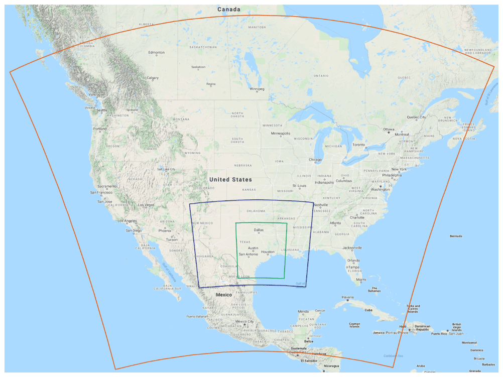
Figure 1CAMx 36, 12, and 4 km modeling domains. The underlaid image is from © Google Maps.
Table 1NOx inventory emission rates for 2019 from the four largest metropolitan areas and three largest power plants within our model domain. For the cities, the fraction of emissions allocated to on-road mobile sources is also noted.
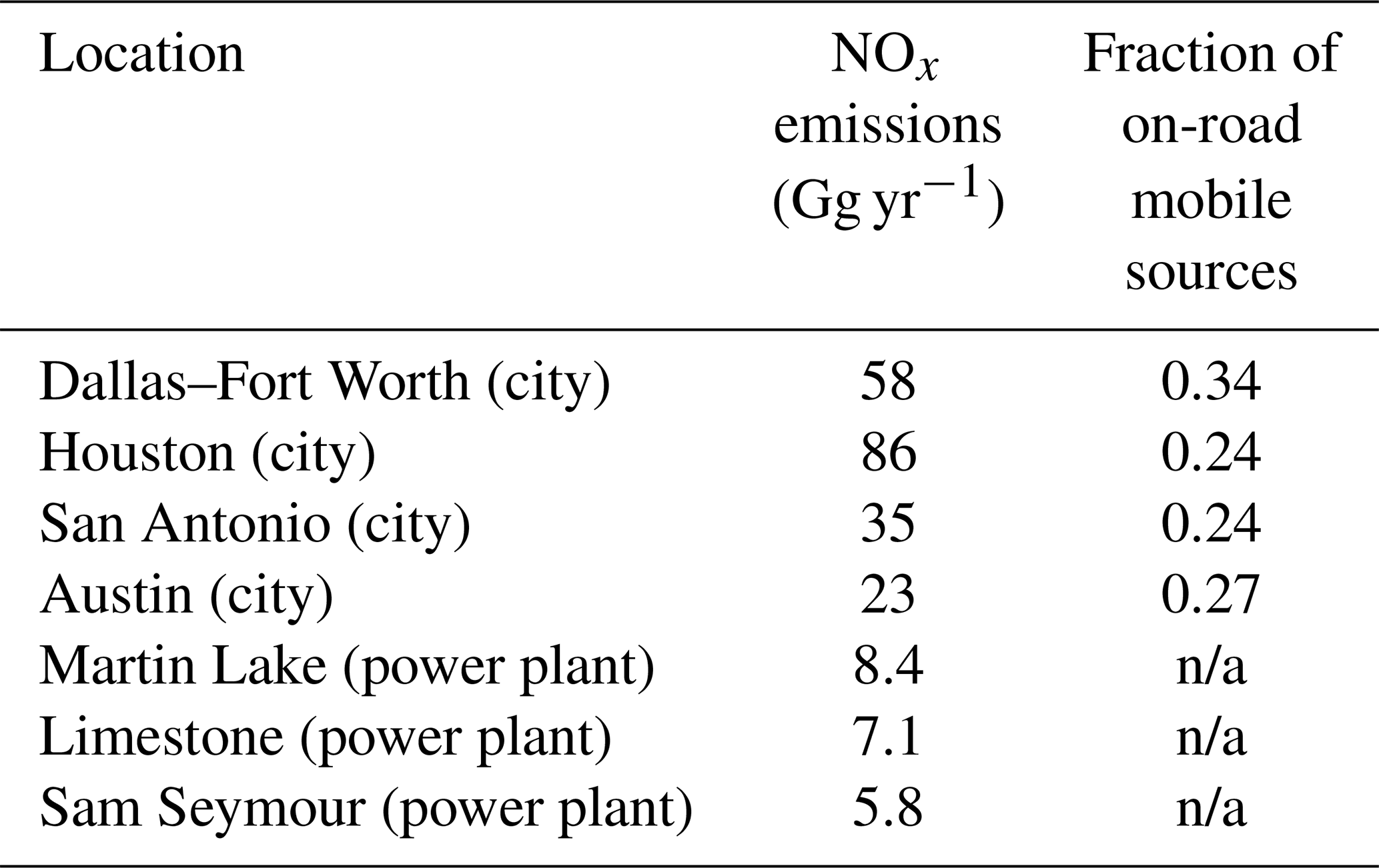
n/a: not applicable.
Biogenic emissions were estimated for 2019 from the Model of Emissions of Gases and Aerosols from Nature (MEGAN) version 3.1 and fire emissions from Fire INventory of NCAR (FINN) version 1. We included lightning NOx (LNOX) emissions, with the CAMx LNOx processor using the 2019 WRF meteorological data. The LNOx processor estimates hourly, grid-column-specific lightning flash rates (Luo et al., 2017; Price and Rind, 1992) using cloud top heights and convective available potential energy (CAPE) diagnosed from WRF temperature and moisture profiles. The processor then determines the ratio of intracloud lightning (IC) to cloud-to-ground lightning (CG) according to the approach of Price and Rind (1993), NO yield per flash estimated by Pickering et al. (2017), and vertical distribution of resulting NO emission rates following DeCaria et al. (2005). In-line inorganic iodine emissions (Ix) from saltwater areas and iodine chemistry are also included.
2.2 TROPOMI
TROPOMI was launched by the European Space Agency (ESA) for the European Union's Copernicus S5P satellite mission on 13 October 2017. The satellite follows a sun-synchronous, low-Earth (825 km) orbit, with an Equator overpass time of approximately 13:30 LST (local solar time). TROPOMI measures total column amounts of several trace gases in the ultraviolet-visible-near-infrared (UV-VIS-NIR; e.g., NO2 and HCHO) and shortwave infrared (SWIR; e.g., CO) spectral regions. At nadir, pixel sizes are 3.5×7 km2 (modified to 3.5×5.5 km2 on 6 August 2019), with the edges having slightly larger pixels sizes (∼14 km wide) across a 2600 km swath, equating to 450 rows (van Geffen et al., 2020). The instrument observes the swath approximately once every second and orbits the Earth in about 100 min, resulting in daily global coverage. For domain-wide comparisons, we screened TROPOMI pixels for quality assurance flag values greater than 0.75. As a polar-orbiting satellite with an afternoon overpass, care must be taken in the interpretation of TROPOMI column retrievals as an indicator of near-surface emissions (Penn and Holloway, 2020; Streets et al., 2013). TROPOMI provides snapshots at the same time each day, except when limited by cloud cover, surface albedo, or instrument errors.
2.2.1 NO2
NO2 slant column densities are derived from radiance measurements in the 405–465 nm spectral window of the UV-VIS-NIR spectrometer. Tropospheric vertical column density data, which represent the vertically integrated number of NO2 molecules per unit area between the surface and the tropopause, are then calculated by subtracting the stratospheric portion and then converting the tropospheric slant column to a vertical column using an air mass factor (AMF). The AMF is a unitless quantity used to convert the slant column into a vertical column and is a function of the satellite viewing angles, solar angles, the effective cloud radiance fraction and pressure, the vertical profile shape of NO2 provided by a chemical transport model simulation (for operational data, the TM5-MP model is used at 1×1∘ resolution; Williams et al., 2017), and the surface reflectivity (for operational data, climatological Lambertian-equivalent reflectivity is used at a 0.5×0.5∘ resolution; Kleipool et al., 2008). The operational AMF calculation does not explicitly account for aerosol absorption effects, which are accounted for in the effective cloud radiance fraction.
For our analysis, we use both the v1.3 offline (OFFL) algorithm, which was operational during the April through September 2019 time frame, and the v2.3.1 Product Algorithm Laboratory (PAL) algorithm, released in December 2021 and includes updates to the cloud retrieval scheme (decrease in cloud pressure), the surface albedo (to avoid negative cloud fractions), and the quality flags (better screening of snow). The net result of the change in tropospheric vertical column NO2 from v1.3 to v2.3.1 has been reported to be a +13 % increase for cloud-free scenes that varies spatially and is higher in polluted areas (van Geffen et al., 2021).
2.2.2 HCHO
HCHO slant column densities are derived from radiance measurements in the 328–359 nm spectral window of the UV-VIS-NIR spectrometer. In a similar manner to NO2, HCHO is measured as a slant column and is converted from a slant column to a vertical column using an AMF and a priori information from TM5-MP. However, in contrast to NO2, HCHO is reported only as a tropospheric vertical column amount since the stratospheric portion is negligible.
For our analysis, we use the v1.1.6 offline (OFFL) algorithm, which was operational during the April through September 2019 timeframe. At the time of this study, there has not been a public release of TROPOMI HCHO data using the version 2 algorithm predating 13 July 2020.
2.2.3 Regridding and accounting for the vertical sensitivity of TROPOMI
For comparison with CAMx, we gridded TROPOMI data to the model to create a custom level 3 data product for comparison either with each other or with model data on a common grid. Though our level 3 data product is on an equivalent horizontal grid as the model, the satellite a priori (used in the retrieval) and CAMx have different vertical resolutions and distributions of NO2. To limit artificial differences when doing the comparisons in this work, additional processing is done in two ways.
-
Applying the averaging kernel. The most user-friendly approach involves creating a model-simulated satellite NO2 column using the CAMx profile and a TROPOMI data-product-specific averaging kernel, which may be described as the weights used to calculate a weighted vertical integral (we refer to this as AK). To apply the averaging kernel to the model simulation, we first interpolate the averaging kernel from the TM5-MP vertical pressure levels to the CAMx vertical pressure levels at each horizontal grid location using linear interpolation. Once the averaging kernel is on the CAMx grid, we multiply the partial tropospheric columns by the averaging kernel at each vertical level (e.g., multiply the partial columns by ∼1.5 at 10 km, by ∼1 at 2 km, and by ∼0.5 near the surface) to account for the retrieval sensitivity at different altitudes. We applied the gridded TROPOMI NO2 averaging kernel in a similar manner to previous work (Deeter, 2002; Harkey et al., 2015, 2020).
-
Recalculating the AMF. In a second approach, we instead use daily partial vertical NO2 columns from CAMx and the tropospheric averaging kernel to recalculate a new TROPOMI AMF, as described in the TROPOMI NO2 Product User Manual (Eskes et al., 2021). The tropospheric slant column is then divided by the recalculated AMF to generate day-specific recalculated tropospheric vertical column NO2 (Goldberg et al., 2017; Judd et al., 2020). This new satellite measurement can then be compared directly to the tropospheric vertical column NO2 from the CAMx model simulation.
2.3 Deriving NOx emissions from TROPOMI NO2
2.3.1 Exponentially modified Gaussian fitting method
To derive NOx emissions from the polluted areas of eastern Texas, an exponentially modified Gaussian (EMG) function is fit to a collection of NO2 plumes observed from TROPOMI. The original methodology, proposed by Beirle et al. (2011), involves the fitting of satellite line densities to an EMG function. Line densities are the integral of the column NO2 retrieval perpendicular to the path of the plume, and the units are mass per distance. We rotate each day's plume based on the wind direction, so that all daily plumes are artificially in the same horizontal direction (Lu et al., 2015; Valin et al., 2013). The 100 m wind speed and direction are obtained from the ERA5 reanalysis project (Hersbach et al., 2020). Appendix B has a sensitivity analysis of using different wind configurations. Once all daily plumes are rotated and aggregated together, the EMG statistical fit can be applied as expressed in Eq. (1):
where α is the total number of NO2 molecules observed near the pollution source, excluding the effect of background NO2 and β. xo is the e-folding distance downwind, representing the length scale of the NO2 decay, µ is the location of the apparent source relative to the assumed pollution source center, σ is the standard deviation of the Gaussian function, representing the Gaussian smoothing length scale, and Φ is the Gaussian cumulative distribution function. Using the CURVEFIT function in IDL (Interactive Data Language), we determine the following five unknown parameters: α, xo, σ, μ, and β, based on the independent (distance; x) and dependent (NO2 column line density) variables.
Using the mean ERA5 100 m wind speed, w, the mean effective NO2 lifetime τeffective, and the mean NOx, emissions can be calculated from the fitted parameters xo and α, as expressed in Eq. (2):
Equation (2) yields emission estimates in units of moles per second. A factor of 1.32 is the mean column-averaged ratio and is the widely used value to convert the NO2 to NOx in polluted regions (Beirle et al., 2021). Appendix C shows the variation in the across our domain.
2.3.2 Flux divergence method
Emissions were also estimated using the flux divergence method, as follows (Beirle et al., 2019):
Fluxes of NO2 were obtained by multiplying NO2 vertical column densities (VCDs) with wind speeds (u) in orthogonal directions (along and across the swath tracks). The divergence of the fluxes yields an emission estimate in units of moles per meter squared per second. The fluxes can then be integrated across the 2-D urban area to obtain emission rates in analogous units as Eq. (2). Sinks of NO2 are included in the equation by adding VCDs divided by the atmospheric lifetime of NO2, τ, which was taken from the EMG fit. Estimates of NOx emissions are obtained by multiplying the estimates by the ratio of NOx to NO2, which is the same 1.32 value as the EMG method (Beirle et al., 2021). The fluxes were calculated using the same 100 m ERA5 wind product used for the EMG estimates. The winds were linearly interpolated to the daily swath grid. This method follows de Foy and Schauer (2022), with minor modifications. The quality assurance flag threshold was set to 0.75 to be consistent with EMG. The central 250 pixels (out of 450) were used for swaths, as these have a higher resolution than the outer bands and are critical for this method. We retrieved swaths from October 2019 through September 2021. Although this period does include the COVID-19 lockdown period, the October 2019 through September 2021 time frame does not show time-averaged NO2 values more than 10 % different than the year prior and is well within the uncertainty of this analysis. Using the method described in de Foy et al. (2014), two-dimensional Gaussian fits were obtained.
3.1 Comparison between TROPOMI version 1.3 and version 2.3.1 algorithms
To elucidate the effects of the recent TROPOMI NO2 algorithm change from v1.3 to v2.3.1, we compare both within our model domain. As expected, the v2.3.1 algorithm yields consistently larger values than the v1.3 algorithm in most areas of our eastern Texas domain (Fig. 2). The largest increases by both magnitude and percentage occur in the most polluted areas. We find an average increase of +16.6 % in urban counties, with a maximum increase of +45 % in the most polluted section of eastern Houston. Increases exceeding +20 % also occur in the vicinity of large point source emissions. In the rural areas of eastern Texas, we generally observe small increases of less than +5 %. We fit a linear regression to a scatterplot of the tropospheric vertical columns from both algorithms in the urban counties and find a slope of 1.30 and a negative intercept, which further confirms that the algorithm change affects the most polluted areas more strongly than the moderate and less polluted areas.
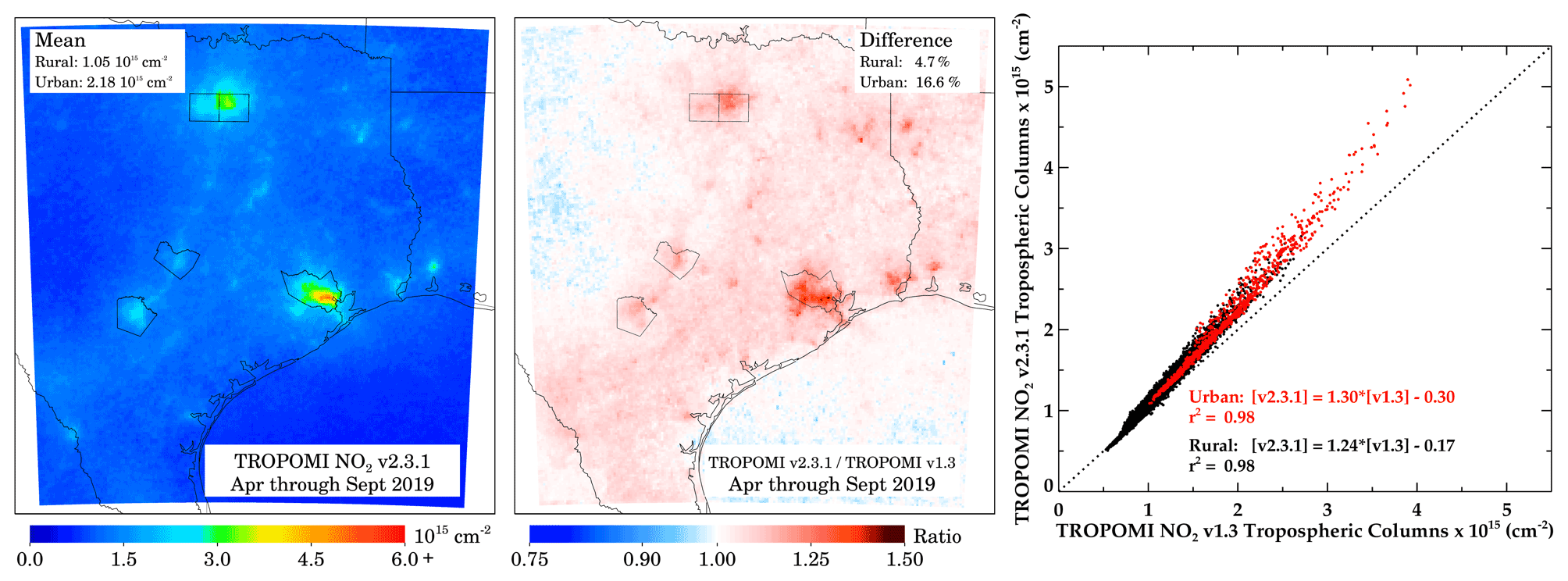
Figure 2The left panel shows the NO2 tropospheric vertical column amounts from the TROPOMI NO2 v2.3.1 algorithm screened with a quality assurance flag greater than 0.75. The center panel shows the ratio between the NO2 tropospheric vertical column amounts from the v2.3.1 algorithm compared to the v1.3 algorithm. The right panel shows a scatterplot and linear fit between the two TROPOMI NO2 products used in the center panel. The urban area is defined as the five counties surrounding the largest five cities (Houston, Dallas, Fort Worth, San Antonio, and Austin). The rural area is everywhere outside those counties.
3.2 Effects of free tropospheric NO2 and lightning NOx
For this study, we conducted two CAMx simulations, i.e., with and without lightning NOx emissions. The tropospheric NO2 vertical profiles for eastern Texas, Dallas, and Houston are shown in the left-hand side panels of Fig. 3. In a CAMx simulation without lightning NOx, average NO2 concentrations between 2.5–10 km averaged 20 ppt (parts per trillion) for the eastern Texas domain. This can be compared to free tropospheric (>2.5 km) NO2 concentrations from the NASA Studies of Emissions, Atmospheric Composition, Clouds and Climate Coupling by Regional Surveys (SEAC4RS) campaign within our eastern Texas model domain but in 2013 instead of 2019. Measured NO2 concentrations between 2.5 and 10 km averaged 50 ppt during the SEAC4RS campaign. This also compares the ∼40 ppt estimate from OMI using a cloud-slicing methodology in the central U.S. during June–August 2005–2007 (Marais et al., 2018). When lightning NOx emissions are included in CAMx, the free tropospheric NO2 between 2.5–10 km increases from 20 to 33 ppt, but there is still a slight underestimate compared to SEAC4RS data between 2.5 and 6 km. The small underestimate shown in the CAMx simulation with lightning NOx emissions compared to the SEAC4RS data in the 2.5–6 km altitude range could be due to the decrease in anthropogenic NOx emissions between 2013 and 2019. Colocated vertical NO2 measurements in time and space would be needed to evaluate this further.
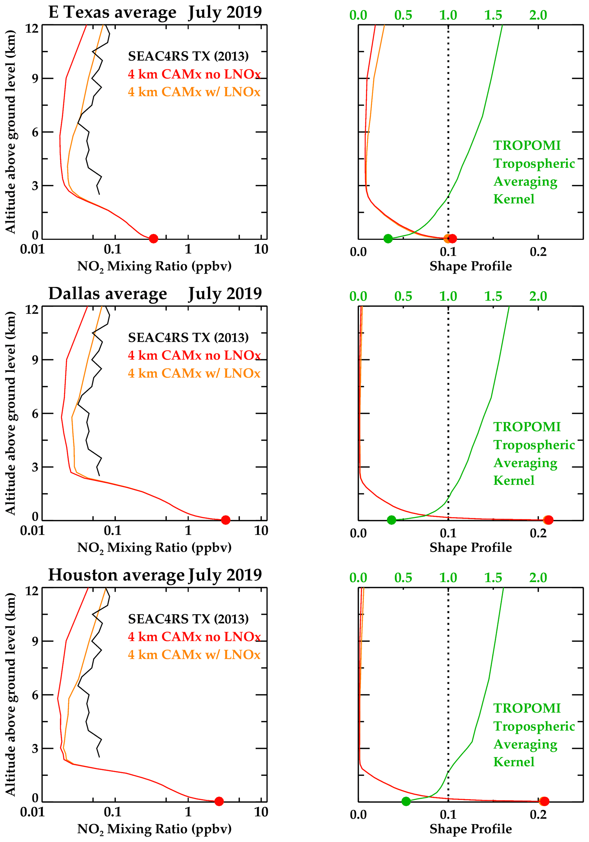
Figure 3The left panels show the NO2 vertical concentration profiles between the surface and 12 km altitude from the CAMx model with (orange) and without (red) lightning NOx emissions for July 2019 and the median free tropospheric NO2 in situ observations acquired during the August–September 2013 NASA SEAC4RS field campaign (black) for (top panels) the eastern Texas average, (middle panels) Dallas, and (bottom panels) Houston. Orange and red dots represent surface concentrations. The right panels show the NO2 shape profiles – the fraction of the column at any given altitude – from the same two model simulations and the TROPOMI tropospheric averaging kernel for the same locations. The dotted line indicates an averaging kernel of 1.
In order to compare model simulation output to satellite data, it is important to understand free tropospheric NO2 (Marais et al., 2018, 2021) and understand its effects on the satellite retrieval (Silvern et al., 2019). TROPOMI has greater sensitivity to the upper portion of the troposphere, and this must be accounted for in any comparison with model output. In the right panels of Fig. 3, we show the modeled shape profiles – the NO2 vertical distribution normalized to a unitless quantity that integrates to unity over the depth of the troposphere – and the sensitivity of TROPOMI to NO2 at different levels of the atmosphere (green line). In Texas during summer 2019, TROPOMI was 3 times as sensitive to NO2 at an altitude of 10 km (tropospheric averaging kernel = 1.5) compared to the surface (tropospheric averaging kernel = 0.5). This demonstrates that NO2 at the tropospheric–stratospheric interface (∼12 km altitude), such as lightning NOx (Zhu et al., 2019) and cruising aircraft emissions, can have an outsized effect on the satellite measurement. To facilitate a comparison, model-simulated column amounts can be adjusted by applying the averaging kernel, which will be discussed in Sect. 3.3.
The inclusion of lightning NOx emissions increases seasonal column tropospheric NO2 by an average of 0.16×10¹⁵ molec. cm−2 in the model simulation during April through September 2019 (Fig. 4). This increase varies spatiotemporally due to the prevalence of thunderstorms; however, when averaged over 6 months, the increase is relatively homogeneous. The inclusion of lightning NOx emissions most affects the satellite–model comparison in rural areas but is also relevant in urban areas. The 0.16×10¹⁵ molec. cm−2 increase yields an increase in the tropospheric column NO2 of +7.8 % in urban areas, +15 % in the rural areas of eastern Texas, and up to +24 % over the Gulf of Mexico. For the rest of this paper, only the CAMx simulation with the inclusion of lightning NOx emissions will be analyzed.
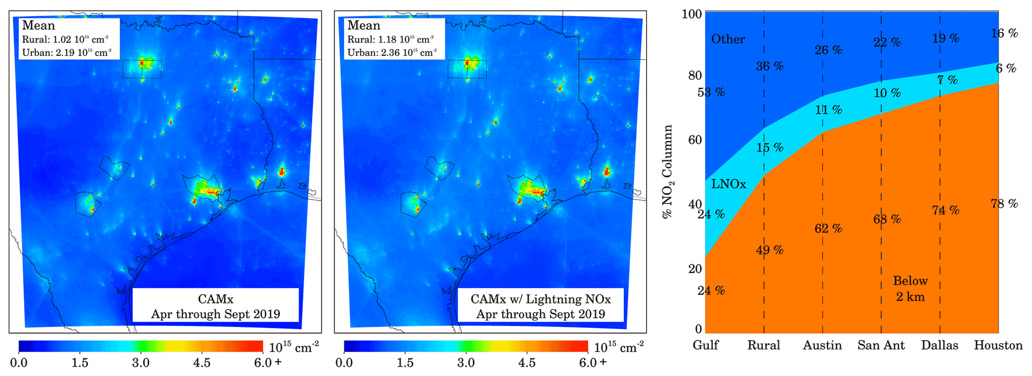
Figure 4NO2 tropospheric vertical column amounts from the CAMx model (left panel) without and (center panel) with lightning NOx emissions averaged during April through September 2019 at the coincident TROPOMI overpass time (∼ 19:00 UTC). Areas with invalid TROPOMI data are similarly screened out from the model output on a daily basis. The urban area is defined as the five counties surrounding the largest five cities (Houston, Dallas, Fort Worth, San Antonio, and Austin). The rural area is everywhere outside those counties. The right panel shows the fraction of the NO2 column attributed to different layers of the atmosphere (below 2 km, above 2 km (attributed to Other), and above 2 km attributed to lightning NOx (LNOx)) at six locations (Gulf of Mexico, rural central Texas, Austin, San Antonio, Dallas, and Houston). The fraction attributed to lightning NOx (LNOx) is calculated as the NO2 addition between the two simulations without and with lightning NOx emissions.
3.3 Applying the averaging kernel and recalculating the air mass factor
To compare a chemical transport model simulation to satellite data, one must account for the differing assumptions about the vertical NO2 distributions between model and satellite. One can either apply the averaging kernel from the satellite instrument to the NO2 column from the model simulation or use the NO2 vertical profile from the model simulation and the averaging kernel to recalculate AMF and tropospheric NO2 vertical column of the satellite measurement. Typically, studies use either one of the two methods; similar to Douros et al. (2022), we use both.
The comparison between the model and model with the tropospheric averaging kernel (AK) applied is shown in the left column of Fig. 5. Upon application of the AK, the tropospheric column NO2 in the model simulation artificially increases in rural areas by +15.4 %, while the urban NO2 will artificially decrease. The latter is due to most NO2 being below 2 km due to the large NOx emissions near the surface in urban areas where AK < 1.
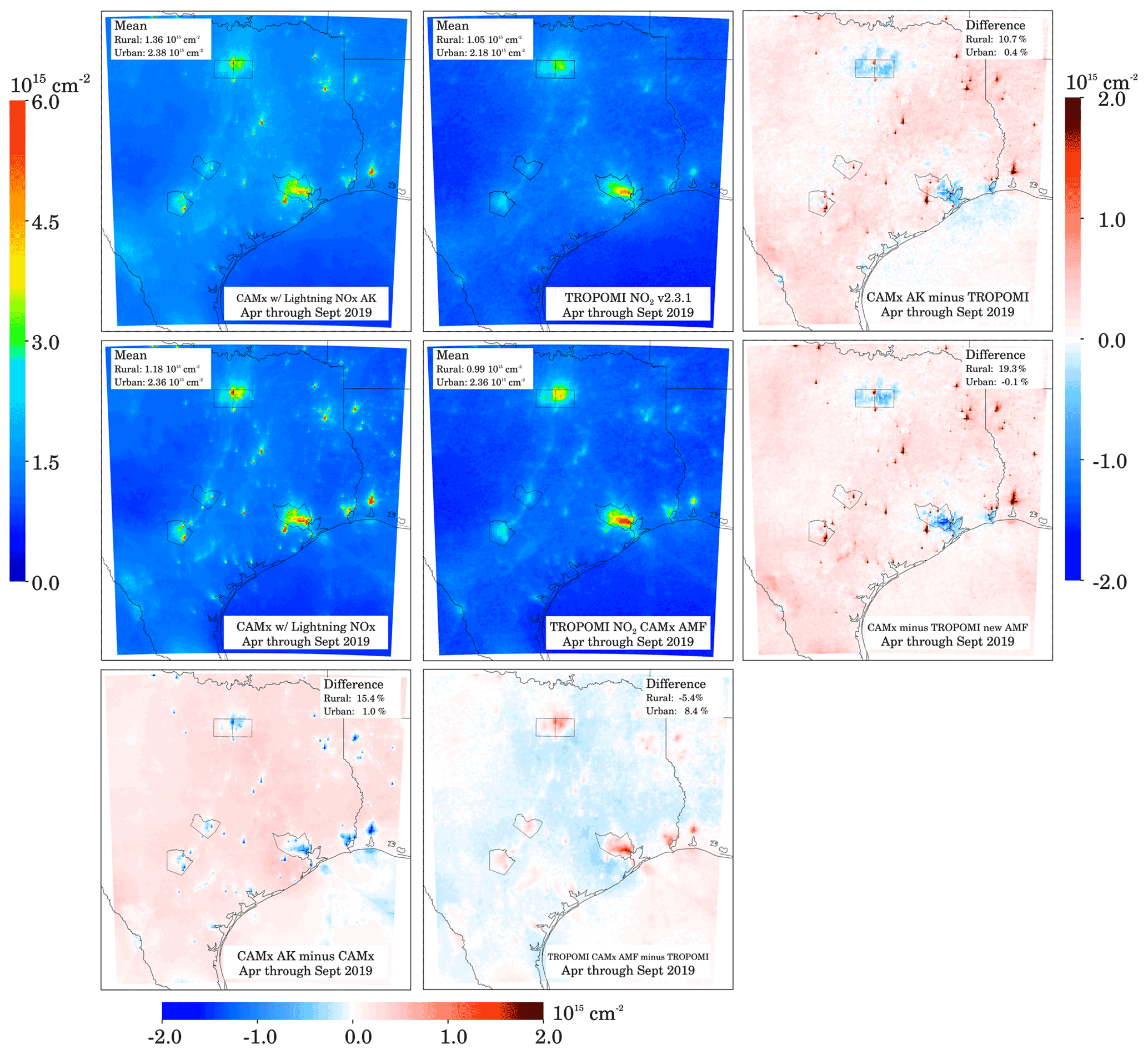
Figure 5The top row panels show the NO2 tropospheric vertical column amounts from CAMx and TROPOMI v2.3.1 reprocessed with a priori profiles from the CAMx model with lightning NOx emissions and the difference averaged across April through September 2019. The middle row panels show the NO2 tropospheric vertical column amounts from CAMx with the averaging kernel applied and the TROPOMI v2.3.1 product and difference averaged across April through September 2019. The bottom row shows the difference between the top and middle rows. Areas with invalid TROPOMI data are similarly screened out from the model out on a daily basis. The urban area is defined as the five counties surrounding the largest five cities (Houston, Dallas, Fort Worth, San Antonio, and Austin). The rural area is everywhere outside those counties.
Once the tropospheric averaging kernel is applied, it can be compared to the satellite directly (top row of Fig. 5). In Dallas–Fort Worth and Houston, there are lower amounts of NO2 in the model simulation in the most polluted areas of the city but generally good agreement (+0.4 %) when the five urban areas (Dallas, Fort Worth, Houston, San Antonio, Austin) are averaged together. In the rural areas of eastern Texas, there are slightly larger amounts (+10.7 %) in the model simulation than that observed by TROPOMI, but these absolute differences are small. The largest disagreements between CAMx and TROPOMI occur in the vicinity of large point sources, which we discuss further in Sect. 3.4
While applying the averaging kernel to a regional model simulation is an appropriate way to compare model simulations with satellite data, it does so by artificially adjusting the high-resolution model simulation to follow the coarse resolution () of the TM5-MP model simulation used to originally process the AMF. Instead, incorporating the high-resolution model vertical profiles in the calculation of the AMF, while more computationally intensive, results in satellite measurements incorporating higher spatial resolution information; in urban areas, this yields satellite measurements that have greater spatial heterogeneity.
In the middle row of Fig. 5, we show a comparison between the model and the satellite with the CAMx-derived AMF. In this comparison, we obtain similar conclusions, as mentioned earlier, in which the model has systematically smaller NO2 amounts than TROPOMI in Dallas–Fort Worth and Houston and larger amounts in rural areas. The agreement between the satellite measurement with a new AMF applied and model simulation is marginally different than when the averaging kernel is applied to the model simulation and compared to the satellite measurement directly. The percentage difference calculations differ primarily because the denominator (i.e., TROPOMI value) is a different magnitude in each case. We attribute this small difference to the rounding errors in the interpolation of the averaging kernel to the CAMx model pressure levels.
3.4 Localized TROPOMI vs. CAMx NO2 comparison
We evaluate two versions of the TROPOMI seasonal average against the CAMx model simulation, i.e., TROPOMI v2.3.1 and TROPOMI v2.3.1 with CAMx AMFs. In Fig. 6, a comparison of these satellite products versus CAMx are shown for the following four metropolitan areas: Dallas–Fort Worth (DFW), San Antonio (SAT), Austin (AUS), and Houston (HOU). Comparing TROPOMI v2.3.1 to CAMx directly without the application of the averaging kernel (which is not recommended) suggests a model high bias of +8.4 % but moderately good association with each other (r2=0.70). We then use the a priori profiles from the CAMx simulation to recalculate the AMF and find that the original model high bias in urban areas becomes a low bias of −0.1 % and becomes a larger low bias in the most polluted sections of the cities (consistent with our discussion in Sect. 3.3). The low model bias is most pronounced in eastern Houston and the downtown area of Dallas. For Dallas–Fort Worth, there also appears to some spatial misallocation because NO2 near the DFW airport is larger in the model than the satellite, while NO2 in the downtown areas of Dallas and Fort Worth is smaller in the model than the satellite. In San Antonio and Austin, there is a small model overestimate, which becomes worse near the large point sources on the periphery of the city. Overall, however, there is a generally good performance between CAMx NO2 and TROPOMI NO2, which is within 20 % in most cases. The value of 20 % is well within the expectation of TROPOMI accuracy and precision. The nonpoint NOx emissions input into the model simulation (e.g., mobile, nonroad, and area sources) are generally within the uncertainty of the satellite measurement, and we would not recommend a substantial alteration to the inventory for these sector emissions, except in the eastern Houston neighborhood. This exercise demonstrates the importance of utilizing the AMF when comparing satellite data to model simulations.
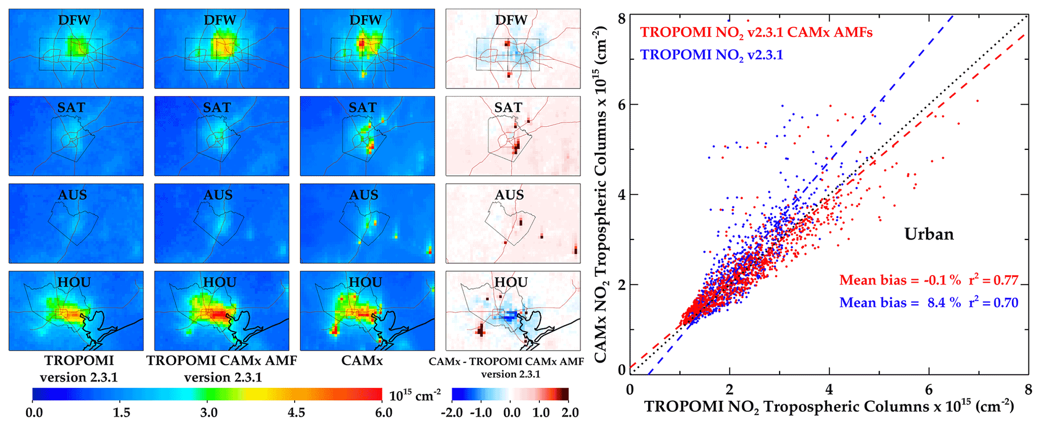
Figure 6The NO2 tropospheric vertical column amounts averaged across April through September 2019 from TROPOMI, TROPOMI v2.3.1, and TROPOMI v2.3.1 with new AMF and CAMx for the largest four metropolitan areas (Dallas–Fort Worth, San Antonio, Austin, and Houston). The right panel is a scatterplot showing the slope and correlation of various TROPOMI configurations and CAMx.
To evaluate the performance of TROPOMI in observing point source emissions, we compare TROPOMI NO2 measurements at the locations of three power plants with stack measurements, i.e., Martin Lake, Limestone, and Sam Seymour (Fig. 7). In each case, TROPOMI substantially underestimates NO2 at the locations of these power plants, even when the new algorithm and recalculated AMF are both applied. We have previously found better agreement between TROPOMI NO2 and the stack measurements for the Colstrip power plant in Montana and San Juan/Four Corners complex in New Mexico (Goldberg et al., 2019b). The reason for the substantial disagreement in Texas is still unknown, but we do not believe this repudiates our prior evaluation for urban areas. NOx emissions from the power sector in the U.S. have declined by 76 % between 2005 (3.63×10⁶ t) and 2019 (0.86×10⁶ t; https://campd.epa.gov/, last access: 24 August 2022). At these lower emission rates, it appears that TROPOMI is having difficulty distinguishing NO2 attributed to power plants from the background NO2 concentrations, especially in areas such as Texas with atmospheric conditions that cause short NO2 lifetimes, i.e., rapid plume dilution, high oxidation capacity due to large numbers of volatile organic compounds (VOCs) and large amounts of water vapor, and high solar elevation angles. Second, the ratio in the model may be underestimated due to the 4 km grid cell size (Appendix C). The two power plants in New Mexico and Montana are located in areas with smaller background NO2, lighter wind speeds, fewer VOCs and less water vapor, and higher elevations; all of these factors cause the satellite sensor to be more sensitive to the NOx emissions. TROPOMI does not have the same difficulty over urban areas because the larger aggregated NOx emissions are more easily distinguishable from background concentrations. Please see Appendix D for a discussion on this topic. Future work should focus on evaluating the NO2 from power plants and the ratio as the plume evolves, such as in situ measurements from aircraft and ground-based vertical column instruments (e.g., Pandora; Herman et al., 2009).

Figure 7The NO2 tropospheric vertical column amounts averaged across April through September 2019 from TROPOMI v2.3.1, TROPOMI v2.3.1 with new AMF, and CAMx for the largest three power plants in eastern Texas, i.e., Martin Lake (lat 32.25∘ N, long 94.58∘ W), Limestone (lat 31.42∘ N, long 96.25∘ W), and Sam Seymour (lat 29.92∘ N, long 96.75∘ W). The right panel is a scatterplot showing the slope and correlation of various TROPOMI configurations and CAMx.
4.1 TROPOMI NOx emissions
In order to calculate NOx emissions directly, we need to account for the NO2 lifetime and NO2 background concentrations. The first technique we use is the exponentially modified Gaussian (EMG) method. We first apply the EMG method to the CAMx simulations of the Limestone power plant (latitude 31.42∘ N, longitude 96.25∘ W) NOx plume. By comparing the known emissions with the inferred top-down emissions, we can evaluate assumptions in the EMG model. The number of NOx emissions input into the model within a 12 km radius of the facility is 9.8 Gg yr−1. The top-down EMG method applied to the CAMx simulation yields a NOx emissions rate of 13.1 Gg yr−1. The disagreement between the NOx emissions inventory (9.8 Gg yr−1) and the inferred CAMx NOx emissions driven by the inventory (13.1 Gg yr−1) must be due to incorrectly assumed effective wind speed likely driven by the meandering of the winds. Winds rarely have a consistent direction and instead meander due to boundary layer turbulence and frictional effects, yielding a slower effective speed in the wind direction over long distances (>10 km). If we assume that the effective speed of the NO2 plume is 25 % slower than the unidirectional wind speed, then the inferred top-down emissions can be made to match the known emissions (9.8 Gg yr−1).
Applying the CAMx-based effective plume speed to analysis of TROPOMI (25 % slower than the unidirectional wind speed), we find that the TROPOMI NO2 v2.3.1 product yields an estimated NOx emissions rate of 5.2 Gg yr−1, and this increased to 6.0 Gg yr−1 when using the TROPOMI v2.3.1 algorithm with a recalculated AMF (Table 2 and Fig. 8). Even with all known corrections applied, it appears that TROPOMI is not capturing the full magnitude of NOx emissions from the power plant and vicinity (9.8 Gg yr−1), which is consistent with the discussion in Sect. 3.4.
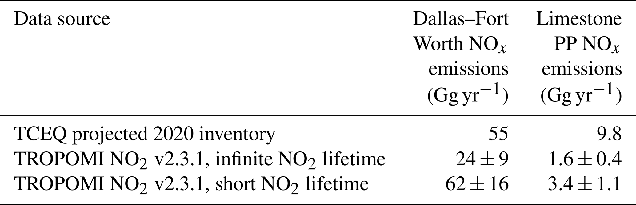
Table 2NOx emission rates for Dallas–Fort Worth and the Limestone power plant from the TCEQ Emissions Inventory and various iterations of the TROPOMI NO2 algorithm.
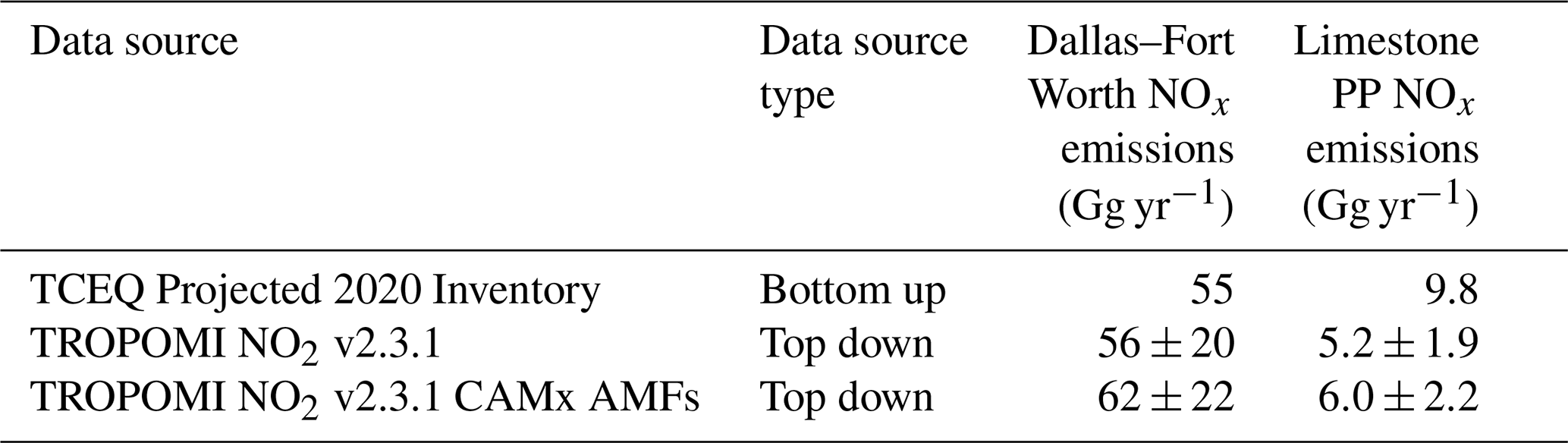

Figure 8EMG method to derive NOx emissions from the TROPOMI NO2 v2.3.1 with CAMx AMFs applied to (left panel) Dallas–Fort Worth and (right panel) Limestone power plant. The color bar for the right panel is halved to better show the NO2 plume near Limestone. ERA5 100 m winds are used to rotate daily TROPOMI NO2 plumes.
For the Dallas–Fort Worth area, if we apply the same method to the CAMx simulation, we obtain an effective NOx emissions rate of 55 Gg yr−1 from the metropolitan area. This is equivalent to the NOx emissions aggregated within a 47 km radius of the Dallas–Fort Worth metropolitan area (latitude 32.85∘ N, longitude 96.95∘ W) and is roughly equivalent to two-sigma of the Gaussian plume (σ=23.7 km).
Using the TROPOMI v2.3.1 algorithm, we calculate a top-down NOx emissions rate of 56 Gg yr−1, and it increases to 62 Gg yr−1 when a CAMx AMF is used (Table 2 and Fig. 8). The difference between the 62 Gg yr−1 calculated directly from the TROPOMI v2.3.1 with a recalculated AMF, and the 55 Gg yr−1 effective emissions rate from CAMx represents a small 13 % low bias that is within the uncertainty of the satellite and the assumptions made to facilitate the comparison. The technique was applied to other urban areas, but those cities have large point sources at the periphery of the urban areas which adversely affected the calculation of the effective NO2 lifetime needed to calculate the NOx emissions.
The top-down approach can also calculate effective NO2 lifetimes. Most top-down methods fit both the effective NO2 lifetime and NOx emissions simultaneously and therefore have a seesaw relationship – as the lifetime increases, the NOx emissions decrease, given a constant NO2 burden. Here, we visually inspect the plume to ensure that the NO2 effective lifetime is reasonable (generally between 0.5–5 h), given the plume decay before proceeding. For Dallas–Fort Worth, the method calculates an effective NO2 lifetime of 1.7 h. The same approach applied to CAMx yields an effective NO2 lifetime of 1.1 h. This suggests that the effective NO2 lifetime in CAMx is too short. The effective lifetime is a function of the chemical lifetime and dispersion lifetime as follows (de Foy et al., 2014):
The effective lifetime could be increased in a model simulation either by increasing the NO2 chemical lifetime (e.g., slower photolysis, slowing the NO2 + OH reaction rate, faster recycling of NOz (NOz = alkyl nitrates, peroxyacyl nitrate (PAN), and HNO3) back to NO2) or by increasing the vertical mixing (less plume meandering at higher altitudes due to fewer surface frictional effects). Chemical NO2 lifetimes are well-constrained by laboratory studies, so we hypothesize that too slow vertical transport may be the primary culprit for this disagreement, and this is also suggested by the analysis presented in Fig. 3, which suggests a low model bias in the free troposphere using measurements from the SEAC4RS campaign. Future vertical NO2 measurements separated by altitude will be critical to answering this question.
The total error associated with the magnitude of the top-down versus bottom-up comparison is calculated to be 36 % and is the sum of the quadrature of five potential sources of error, namely the tropospheric vertical column measurement in urban areas (20 %), the wind speed and direction (25 %; Appendix B), the clear-sky bias (10 %), which for these purposes is a result of emissions being different on clear-sky days compared to cloudy days, the ratio (10 %; Appendix C), and the random error of the statistical EMG fit (10 %; de Foy et al., 2014). This total uncertainty is approximately 20 % smaller than similar methods using OMI. For further information on this method or the uncertainties associated with this method, please see the other literature (de Foy et al., 2014; Goldberg et al., 2019a; Lu et al., 2015; Verstraeten et al., 2018).
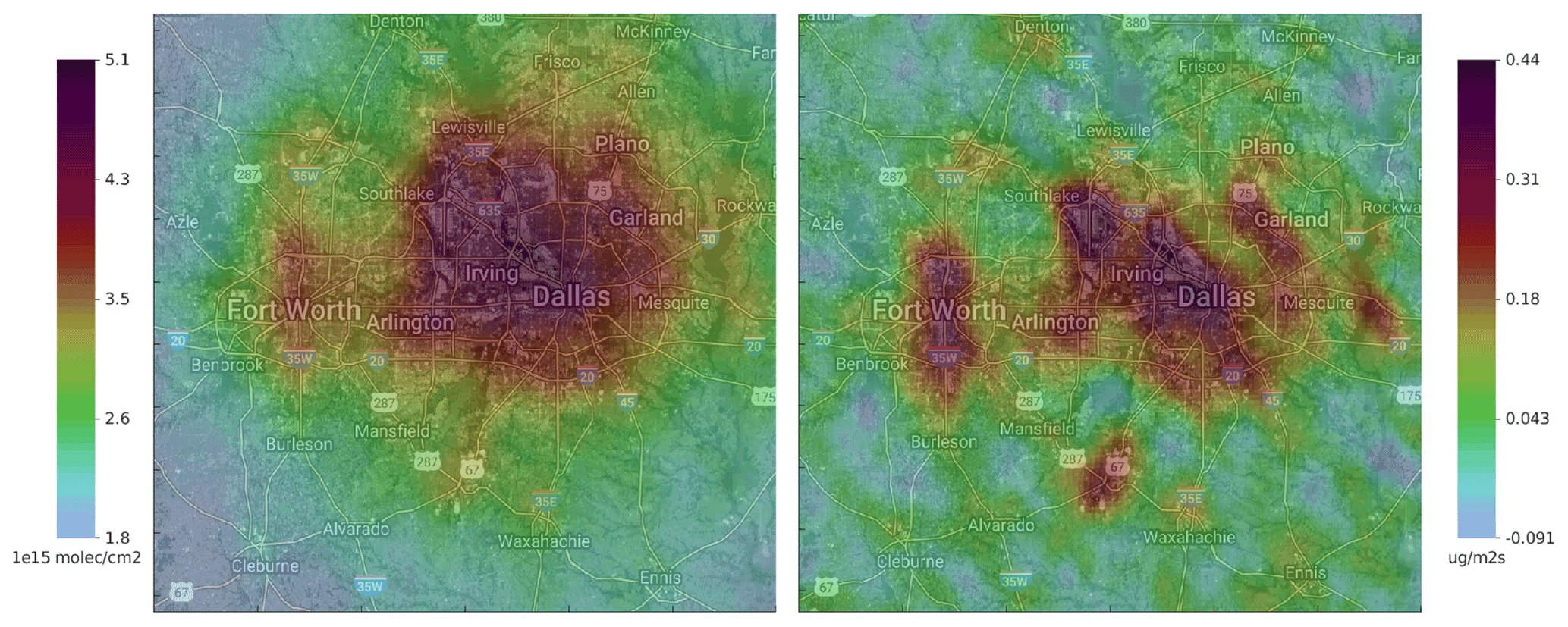
Figure 9Oversampled TROPOMI NO2 in the Dallas–Fort Worth metropolitan areas using the (left panel) tropospheric vertical columns and (right panel) the flux divergence of the tropospheric vertical columns. The underlaid image is from © Google Earth.
We then test the flux divergence method (Beirle et al., 2019, 2021; de Foy and Schauer, 2022) on the same two sources, i.e., Dallas and the Limestone power plant. We apply the flux divergence method to the native TROPOMI pixels rather than a regridded version of the data. Figure 9 shows that TROPOMI columns distinguish between a large hotspot over Dallas and a smaller one over Fort Worth. For the Dallas urban area, the algorithm identified 11 separate source regions which were each represented by a separate two-dimensional Gaussian method. The flux divergence method was able to resolve source regions with better detail, with estimates for some of the individual point sources and sub-areas within Dallas. In particular, the area including the Dallas/Fort Worth International Airport appears as a distinct source area. In Table 3, we show the NOx emissions aggregated for these two sources, using both an infinite NO2 lifetime and the effective short NO2 lifetime provided by the EMG method (τ=1.7 h for Dallas–Fort Worth; τ=0.5 h for Limestone PP). The results from the flux divergence method are consistent with the results from the EMG method in the Dallas area, provided that a short NO2 lifetime is assumed.
Table 3NOx emission rates for Dallas–Fort Worth and the Limestone power plant from the TCEQ Emissions Inventory and various iterations of the flux divergence method using the TROPOMI NO2 v2.3.1 algorithm.
4.2 Evaluating ozone sensitivity using the HCHO–NO2 ratio
Satellite observations of formaldehyde (HCHO) can be combined with NO2 to determine the ozone sensitivity to NOx emissions using the formaldehyde to nitrogen dioxide column density ratio (FNR; Duncan et al., 2010; Jin et al., 2017; Jin and Holloway, 2015; Martin et al., 2004). HCHO may be used to estimate short-lived VOC emissions, both anthropogenic and biogenic combined, which often quickly oxidize to HCHO in the presence of sunlight and the hydroxyl (OH) radical (Wolfe et al., 2016; Zhu et al., 2017). In a similar manner to NO2, column HCHO can be compared to chemical transport models in order to better understand the spatial variability in VOC emissions. Harkey et al. (2020) found that a regional model captured the general spatial and temporal behavior of satellite estimates but tended to underestimate column HCHO. In the western U.S., TROPOMI HCHO measurements have been rigorously evaluated using ground-based spectrometers, and the v1.1 algorithm was found to be biased low by approximately 25 % (De Smedt et al., 2021).
We first compare the column HCHO comparison between CAMx and TROPOMI. Tropospheric column TROPOMI HCHO measurements using the v1.1 algorithm are biased low by approximately 25 % (De Smedt et al., 2021). We then create a bias-corrected (b-c) product (multiply by a factor of 1.25) to account for this low bias. In Fig. 10, we compare the operational TROPOMI HCHO v1.1 product and TROPOMI HCHO v1.1 b-c product to CAMx tropospheric column amounts with and without the averaging kernel sampled at coincident timeframes. Since HCHO spatial patterns have less heterogeneity than NO2, due to a large fraction of HCHO originating from biogenic precursors during warm season months, column HCHO amounts are less sensitive to the application of the AK than with NO2. The difference between CAMx and CAMx with the averaging kernel applied is ±2.5 % for area-wide averages. CAMx underestimates HCHO in central and western Texas, but in eastern Texas the magnitude and spatial patterns match better. The model bias is −7.9 % in eastern Texas and −25.0 % in central Texas, compared to the TROPOMI HCHO v1.1 b-c product. This model bias, in both cases, is within the uncertainty of the satellite retrieval.
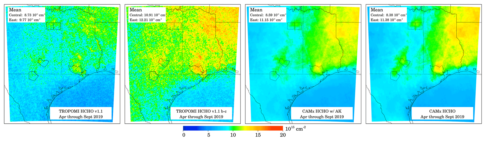
Figure 10HCHO tropospheric vertical column amounts averaged across April through September 2019 from (a) TROPOMI, (b) the TROPOMI bias-corrected model, (c) the CAMx regional model with the TROPOMI averaging kernel (AK) applied, and (d) CAMx without the AK applied. All model information is shown at the coincident TROPOMI overpass time (∼ 19:00 UTC). Areas with invalid TROPOMI data are similarly screened out from the model out on a daily basis. The eastern and central Texas areas are denoted by the dashed lines.
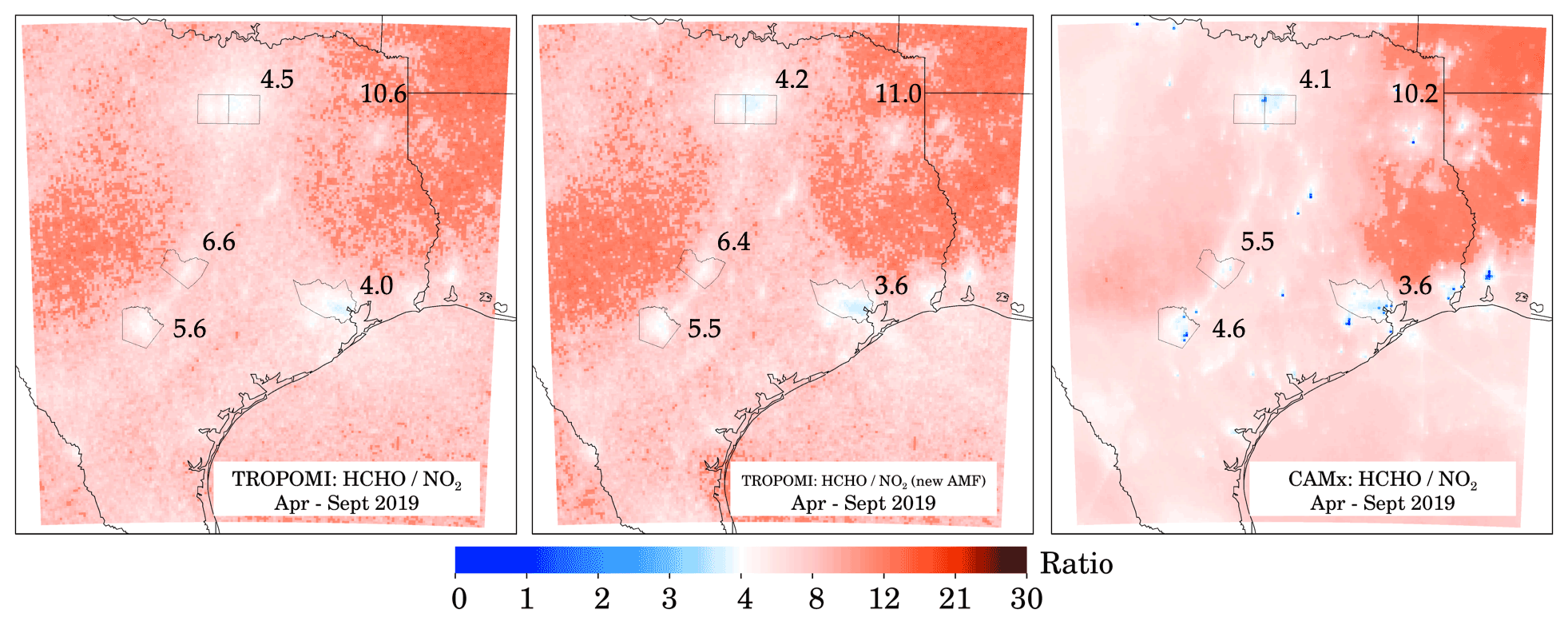
Figure 11The formaldehydeNO2 ratio (FNR) in Texas averaged across April through September 2019, using the (left panel) operational TROPOMI products, (center panel) operational TROPOMI HCHO product and TROPOMI NO2 product with new AMFs, and (right panel) CAMx column amounts. Only CAMx data coincident with the overpass time and valid TROPOMI pixels are included. The ratios from the satellite and model for each area are shown directly in the plot.
We apply the FNR to TROPOMI and CAMx to determine how well CAMx is representing ozone formation regimes. Initial studies showed that, when the FNR in a region exceeds 2, the ozone formed is considered to be limited by the amount of NOx present in the air. When the FNR is below 0.5, the ozone formed is considered to be limited by the amount of VOCs. Ratio values between 0.5 and 2 indicate sensitivity to both NOx and VOCs (Duncan et al., 2010). More recent studies have demonstrated that the upper bound of the transitional regime could be as high as 4 (or even higher), depending on regional characteristics (Jin et al., 2017, 2020; Schroeder et al., 2017).
For this analysis, using the v1.1 HCHO and v1.3 NO2 algorithms is sufficient, since both products have similar biases related to the cloud schemes that may cancel out when a ratio is calculated. We use a value of 4 to indicate the transition between NOx and VOC sensitivity, while simultaneously noting that this value should not be static in all scenarios. In Fig. 11, the ratios from the satellite and model for each area are shown directly in the plot.

Figure 12Diurnal cycles of column NO2, column HCHO, and the ratio from CAMx for these regions in our model domain, i.e., Houston, Dallas–Fort Worth, and rural eastern Texas (Cass County). The approximate TROPOMI overpass time of 13:30 LT (local time) is denoted by the dotted line.
On a regional scale, there is excellent spatial agreement between the satellite and model. Ozone formation conditions are NOx limited (FNR > 4) throughout the vast majority of Texas; other studies have found similar conclusions within the last 5 years (Jin et al., 2020; Koplitz et al., 2021). Only along the Houston Ship Channel, near the DFW airport, and in the presence of undiluted power plant plumes are conditions potentially in the transitional regime. When aggregated on an urban scale, the model ratio values are marginally lower than the satellite-derived ratios, especially in San Antonio and Austin. This low model bias is improved when the AMF of the NO2 product is recalculated. Consistent with the analyses presented in Sect. 3.3 and 3.4, the model appears to be capturing both the HCHO and NO2 spatial patterns with satisfactory performance, and therefore, the ozone production regimes are also captured well. The only areas of strong disagreement are in the presence of power plant plumes and large point sources, which TROPOMI appears to be not fully characterizing.
The downside of low-Earth orbiting instruments is the consistent measurement during the early afternoon. This early afternoon measurement time coincides with (1) a temporary dip in NOx emission rates, which are largest in the early morning and late afternoon, (2) the peak of the biogenic VOC emissions, which often peak at the time of the maximum daily 2 m temperature, and (3) stronger photolysis rates, which affect both NO2 and HCHO.
We use the CAMx model to investigate the temporal variation in the FNR. In Fig. 12, we show diurnal cycles of column NO2, column HCHO, and the FNR. The NO2 diurnal cycle has a minimum in the early afternoon, driven mostly by the higher photolysis rates and, second, by the relatively lower NOx emission rates compared to the early morning and late afternoon. HCHO has broad peak in the afternoon, which is likely related to biogenic emissions and secondary formation. However, the HCHO diurnal cycle is flatter than we expected; this may be due to model difficulties in representing complex VOC chemistry for secondary HCHO production (Schroeder et al., 2016; Schwantes et al., 2022).
According to CAMx, the FNR has a temporary maximum in urban areas around 14:00 LT and a minimum around 08:00 LT, with a secondary minimum around 20:00 LT. In the rural areas of eastern Texas, the variation in the FNR is even more substantial than in the urban areas, and even in these rural areas, ozone production might be VOC limited during early morning hours. Therefore, an early afternoon satellite measurement suggesting NOx-limited conditions does not eliminate the possibility of VOC-limited ozone formation conditions in the early morning. This suggests that targeted VOC controls in urban areas of Texas between 06:00–10:00 LT could be an effective way to further reduce ozone concentrations, in addition to expanded NOx controls at all hours. Upcoming observations from the Tropospheric Emissions Monitoring of Pollution (TEMPO) instrument, which will be located in geostationary orbit, will further help answer this question.
In this study, we find that TROPOMI NO2 columns offer a valuable means to validate NOx emissions inventories, with important limitations. When using locally resolved inputs, simulated urban NO2 columns in Texas agree with TROPOMI to within 20 % in most areas. Using data from the newest TROPOMI NO2 algorithm (v2.3.1) generally showed better agreement with the model. We find some evidence that NOx emissions in certain sections of Dallas–Fort Worth, TX, and Houston, TX, may be underestimated, but the underestimates are within the uncertainty of the methods presented herein.
In the rural areas of eastern Texas, we find generally good agreement to within 20 % in most circumstances between the model and TROPOMI NO2 when lightning NOx emissions are included. In rural regions of eastern Texas, >50 % of the column NO2 appears to be above 2 km in altitude, demonstrating the influence of the free tropospheric NO2, including lightning. Lightning NOx emissions can represent up to 24 % of the column NO2 in our eastern Texas domain and presumably would be larger in more isolated tropical regions. Since free tropospheric NO2 has an outsized effect in rural areas, it is critical to have an accurate estimate of free tropospheric NO2 before conducting a model to satellite comparison in these regions (Shah et al., 2022). More aircraft measurements between the top of the boundary layer and the stratosphere–troposphere interface would be helpful to better understand and quantify free tropospheric NO2.
Over large power plant plumes, however, we find statistically significant differences between the model and satellite measurements. Because the NOx emissions from these power plants are directly measured, we conclude that TROPOMI cannot distinguish NO2 attributed to power plants from the background NO2 concentrations in Texas. This limitation may be due to short NO2 lifetimes characteristic of that region and, second, the ratio in the 4 km model simulation. More work should be dedicated to investigating NO2 and NOy partitioning near power plant plumes, including aircraft and vertical profilers (e.g., Pandora).
In our comparison between TROPOMI and modeled HCHO, we find excellent agreement in far eastern Texas and the Ozarks but an underestimate in central Texas. This is consistent with Harkey et al. (2020), who showed a model underestimate in the western U.S. More work should be done to evaluate HCHO and VOCs in areas with assumed small amounts of biogenic emissions.
In a last step, we evaluate the ozone formation regimes at the time of the early afternoon TROPOMI overpass. We find that ozone production is NOx limited almost everywhere in the domain, except near the Houston Ship Channel, near the DFW airport, and in the presence of power plant plumes. There are likely NOx-saturated ozone formation conditions in the early morning hours that TROPOMI cannot observe.
We are encouraged by the future observational strategies that could help tackle some of the remaining questions presented herein. In early 2023, TEMPO will be acquiring column NO2 and HCHO measurements during all daylight hours in the presence of low amounts of clouds. When coupled with the current ground monitoring network, this will elucidate some of the unknown NO2 and HCHO diurnal cycles, giving us more confidence in our understanding of NOx emissions, NO2 chemistry, and satellite retrievals.
We evaluated CAMx NOx and ozone surface concentrations using data collected at TCEQ Continuous Ambient Monitoring Stations (CAMSs). We evaluated the performance by five geographical subregions, namely Austin, San Antonio, Waco, Tyler, and Dallas–Fort Worth. NOx monitors deployed for routine monitoring have limitations for NO2. These monitors measure NO, and consequently, NO2 is chemically converted to NO for measurement. The converter also captures other compounds, including PAN and a portion of HNO3 (Dickerson et al., 2019). These NOx monitors have a detection limit of around 1 ppb (parts per billion), but differentiation between NO and NO2 is less accurate near the detection limit. Therefore, we compare both CAMx NOx (i.e., NO + NO2) and NOy (i.e., NO + NO2 + PAN compounds + HNO3) to monitored NOx in Fig. A1. Hourly ozone measurements were aggregated to 8 h maximum daily averages (MDA8), and hourly NO2 measurements were aggregated to early afternoon averages (12:00–15:00 CST) to correspond with the TROPOMI overpass time.
Figure A1 displays the O3 and NO2 performance in the CAMx simulation compared to ground monitors. High observed NOx detected by ground monitors in urban areas (e.g., >10 ppb) are not resolved at the 4 km CAMx horizontal grid resolution. As discussed in Souri et al. (2022), care is needed when comparing pointwise measurements to concentrations spatially averaged over large (>1 km) grid cells. For example, Dallas, Hinton St. (CAMS 0401), is located 0.9 km from a major freeway interchange and 200 m from a busy road (Mockingbird Lane). In contrast, Tyler Airport Relocated (CAMS 0082) is in a rural location, removed from busy roads, and the nearby airport is regional and not highly trafficked. When compared with monitored NOx in less polluted areas (i.e., <10 ppb), CAMx NOx tends to be lower than measured NOx, whereas CAMx NOy tends to be higher than measured NOx. We therefore conclude that CAMx is consistent with the ambient NOx measurements within the limitations of the monitoring equipment capabilities and siting.
We present similar scatterplots for maximum daily 8 h average (MDA8) ozone in Fig. A1. CAMx shows skill in identifying low and high ozone days, with R2 values from 0.56 (Austin) to 0.61 (Tyler). CAMx displays a positive ozone bias across all five regions, with the mean bias (MB) ranging from 4.8 ppb (Waco) to 10.1 ppb (San Antonio). Emery et al. (2017) define the criteria standards for MDA8 ozone as ±15 % for normalized mean bias (NMB) and <25 % for normalized mean error (NME). Only Waco and Dallas–Fort Worth meet the criteria standard for NMB, while all regions, except San Antonio, meet the criteria standard for NME.
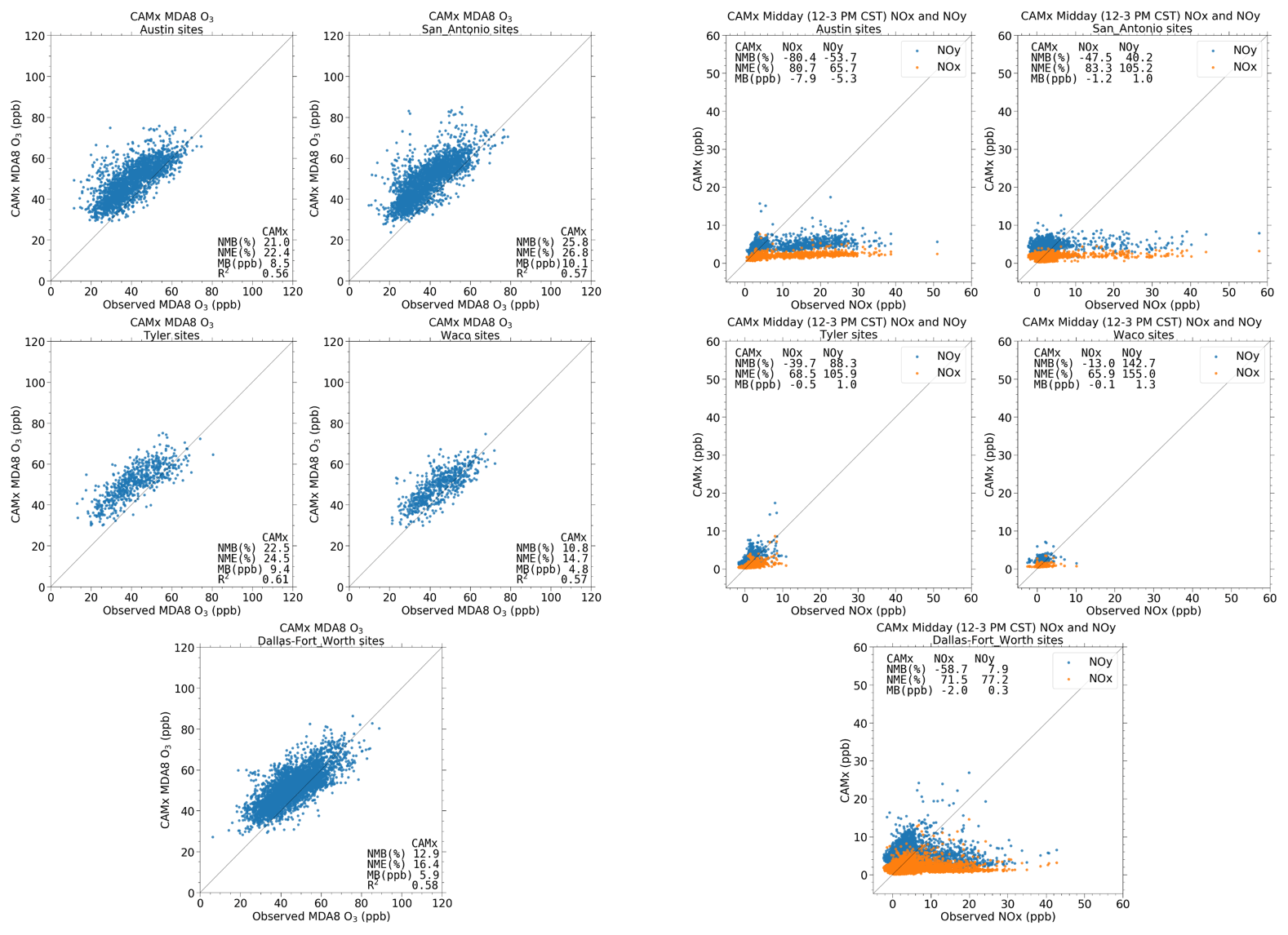
Figure A1CAMx model performance for (left) maximum daily averaged 8 h ozone (MDA8 O3) and (right) midday 12:00–15:00 LT (local time) NOx and NOy. The model output is compared to the EPA Air Quality System (AQS) ground observations for the five regions of interest in our eastern Texas domain (Austin, San Antonio, Tyler, Waco, and Dallas–Fort Worth).
To justify the use of the ERA5 100 m winds (as opposed to another vertical level or interval), we use the NO2 column information from CAMx to determine the weighted-column midpoint. Using the shape profiles described in Fig. 3, we find that 50 % of the tropospheric NO2 column in the Dallas–Fort Worth area is below 227 m in altitude (and therefore 50 % is above this); this is the weighted-column midpoint. Using the WRF simulation, we find that the 100 m wind speed is 6 % slower than the 227 m wind speed in Dallas–Fort Worth. However, as we discuss in Sect. 4.1, errors due to wind meandering (∼25 %) are far more critical.
We can then apply uncertainty bounds to this. In the most polluted sections of the city, the column midpoint would be lower (tens of meters), and in the least polluted sections of the city, the column midpoint can be as high as 500 m. While neither of these are appropriate for an area-wide average, they can constrain the uncertainties of the column midpoint. Using the WRF simulation, we find that winds at 500 m are 15 % faster and surface winds are 24 % slower than the 100 m wind speed (Table B1).
Table B1Wind speeds at Dallas–Fort Worth for the April–September 2019 average at various vertical levels in comparison to the 100 m wind speed.

To further investigate whether the ratio used in our study is appropriate, we probe the CAMx simulation to calculate the ratio for the partial columns below 2 km (Fig. C1). The ratio above 2 km is inappropriate for use in the EMG method since the column above 2 km represents background conditions and is subtracted out when using the EMG method.
The ratio for the partial column below 2 km in urban areas is 1.31±0.02 (Dallas is 1.33, Austin is 1.30, San Antonio is 1.32, and Houston is 1.295). For urban areas, this represents an uncertainty in the ratio of less than 10 %. Our original assumption of using a ratio of 1.32 is warranted.
However, the ratio can vary more substantially near large point sources. In the grid cells of the large point source itself, the ratio can be as large as 1.52. It is possible that the ratio in the model may be underestimated due to the emissions being equally spread out across the 4 km grid cell. ratios can be as large as 2 within 100 m downwind of major NOx sources, especially under low ozone (<30 ppb) conditions (Kimbrough et al., 2017). However, further downwind (>4 km) of these large point sources, the ratio quickly converges back to a value of ∼1.31.

Figure C1The ratio at 13:00 LT for April–September 2019 for partial NO2 columns below 2 km in altitude, as simulated by CAMx.
Daily images of the TROPOMI NO2 vertical column densities are shown in Fig. D1. The top set of panels shows the daily images over Dallas–Fort Worth during July 2019. These daily images document that a NO2 plume can be observed on every day on which there are no clouds. We also plot the daily ERA5 wind speed and direction on each daily panel. ERA5 winds appear to correctly identify the urban plume direction on each day.
The middle set and bottom set of panels (Martin Lake, TX, and Colstrip, MT, respectively), demonstrate the capability of TROPOMI of observing daily plumes from power plants during July 2019. For Colstrip (13 600 t NOx yr−1), a plume signature can be visually located on every cloud-free day. However, in Martin Lake, TX (9500 t NOx yr−1), a plume signature cannot be visually located on every cloud-free day, even though NOx emissions are of a similar order of magnitude as in Colstrip. This suggests that the location and atmospheric conditions in Texas are causing TROPOMI to not fully observe Martin Lake's NOx emissions.
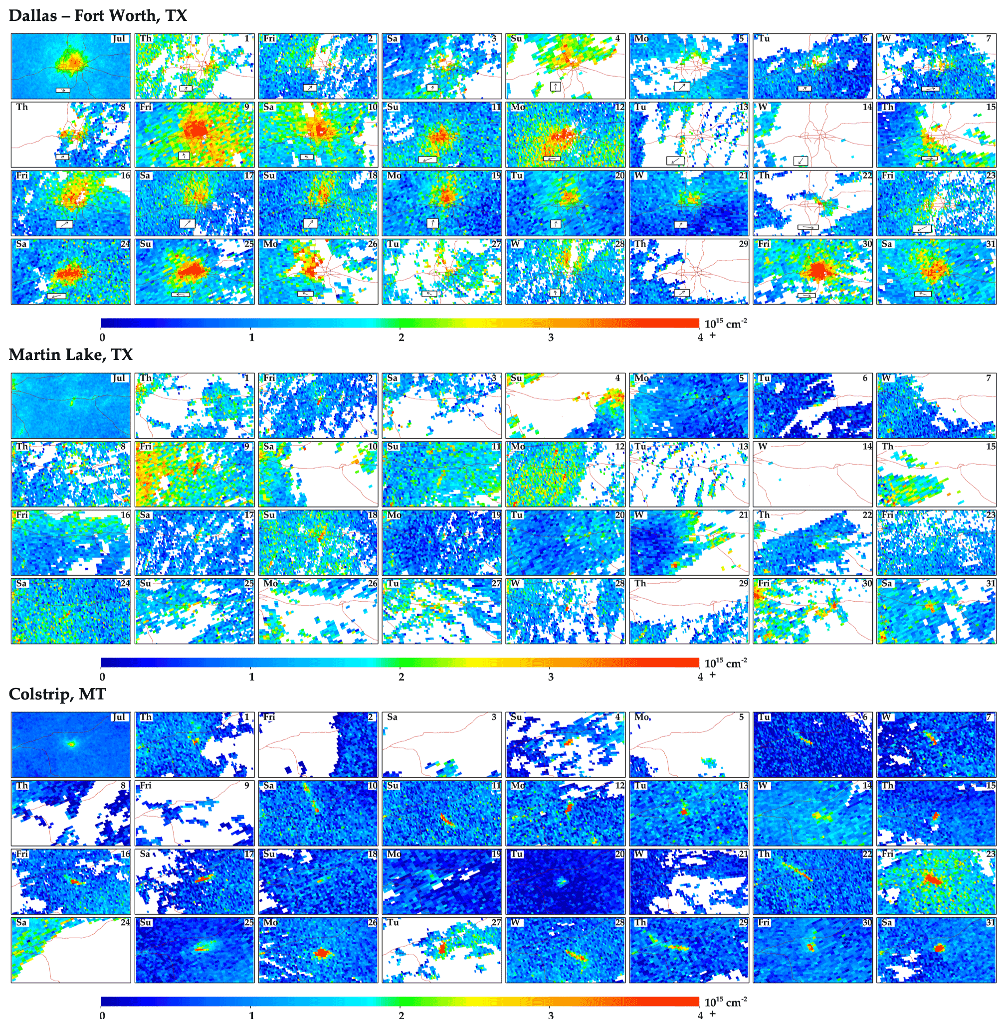
Figure D1Daily TROPOMI NO2 vertical column densities over three locations (Dallas–Fort Worth and Martin Lake and Colstrip power plants) during each day of July 2019; the July 2019 monthly average is denoted in the top left panel of each location aggregate.
TROPOMI NO2 v1.3 data (https://doi.org/10.5270/S5P-s4ljg54; European Space Agency, 2019) and TROPOMI HCHO v1.1 data (https://doi.org/10.5270/S5P-tjlxfd2; European Space Agency, 2022a) can be freely downloaded from the Copernicus Open Access Hub (https://s5phub.copernicus.eu/dhus/; European Space Agency, 2022b) or NASA Earthdata Hub (https://disc.gsfc.nasa.gov/datacollection/S5P_L2__NO2____1.html; National Aeronautics and Space Administration, 2022a; https://disc.gsfc.nasa.gov/datacollection/S5P_L2__NO2____HiR_1.html; National Aeronautics and Space Administration, 2022b; https://disc.gsfc.nasa.gov/datacollection/S5P_L2__HCHO___1.html; National Aeronautics and Space Administration, 2022c; and https://disc.gsfc.nasa.gov/datacollection/S5P_L2__HCHO___HiR_1.html; National Aeronautics and Space Administration, 2022d). TROPOMI NO2 v2.3.1 data can be freely downloaded from the S5P-PAL Data Portal (https://data-portal.s5p-pal.com/products/no2.html; European Space Agency, 2022c). NASA SEAC4RS data can be downloaded from NASA Data Archive (https://doi.org/10.5067/Aircraft/SEAC4RS/Aerosol-TraceGas-Cloud; National Aeronautics and Space Administration, 2022e) and was acquired by the UC Berkeley Cohen research team. ERA5 reanalysis hourly data on single levels (https://doi.org/10.24381/cds.adbb2d47; Copernicus Climate Data Store, 2022a) can be downloaded from Copernicus Climate Data Store (https://cds.climate.copernicus.eu/#!/home; Copernicus Climate Data Store, 2022b). The IDL code to regrid and process the data is available upon request.
DLG processed the satellite data, produced most of the figures, and wrote the paper. MH, BdF, and LJ provided guidance with the processing of the satellite data and helped to develop several of the figures. JJ performed the model simulation, processed the model output, and compared the model simulation to the ground monitors. GY and TH conceptualized the study, obtained funding, and provided guidance and feedback throughout. All authors helped to edit the text of the paper.
The contact author has declared that none of the authors has any competing interests.
Publisher's note: Copernicus Publications remains neutral with regard to jurisdictional claims in published maps and institutional affiliations.
The findings, opinions, and conclusions are the work of the authors and do not necessarily represent findings, opinions, or conclusions of the AQRP or the TCEQ.
The authors would like to thank the reviewers at TCEQ for their input on the paper. We appreciate feedback from Ron Cohen, on the usage of the SEAC4RS data, and Ted Russell, on the intercomparison near power plants.
This preparation of this work has been funded by the Texas Air Quality Research Program (AQRP; grant no. 20-020) at the University of Texas at Austin through the Texas Emission Reduction Program (TERP) and the Texas Commission on Environmental Quality (TCEQ). This project has also been funded by grants from the NASA Health and Air Quality Applied Sciences Team (HAQAST, grant no. 80NSSC21K0511), NASA Health and Air Quality (HAQ, grant no. 80NSSC19K0193), and the NASA Atmospheric Composition Modeling and Analysis Program (ACMAP, grant no. 80NSSC19K0946). For the AQRP funding of this project, Daniel L. Goldberg was paid as a consultant through Ramboll.
This paper was edited by Jeffrey Geddes and reviewed by two anonymous referees.
Bauwens, M., Compernolle, S., Stavrakou, T., Müller, J. -F., Gent, J., Eskes, H. J., Levelt, P. F., van der A, R., Veefkind, J. P., Vlietinck, J., Yu, H., and Zehner, C.: Impact of coronavirus outbreak on NO2 pollution assessed using TROPOMI and OMI observations, Geophys. Res. Lett., 47, e2020GL087978, https://doi.org/10.1029/2020GL087978, 2020.
Beirle, S., Boersma, K. F., Platt, U., Lawrence, M. G., and Wagner, T.: Megacity Emissions and Lifetimes of Nitrogen Oxides Probed from Space, Science, 333, 1737–1739, https://doi.org/10.1126/science.1207824, 2011.
Beirle, S., Borger, C., Dörner, S., Li, A., Hu, Z., Liu, F., Wang, Y., and Wagner, T.: Pinpointing nitrogen oxide emissions from space, Sci. Adv., 5, eaax9800, https://doi.org/10.1126/sciadv.aax9800, 2019.
Beirle, S., Borger, C., Dörner, S., Eskes, H. J., Kumar, V., De Laat, A., and Wagner, T.: Catalog of NOx emissions from point sources as derived from the divergence of the NO2 flux for TROPOMI, Earth Syst. Sci. Data, 13, 2995–3012, https://doi.org/10.5194/essd-13-2995-2021, 2021.
Boersma, K. F., Jacob, D. J., Eskes, H. J., Pinder, R. W., Wang, J., and Van Der A, R. J.: Intercomparison of SCIAMACHY and OMI tropospheric NO2 columns: Observing the diurnal evolution of chemistry and emissions from space, J. Geophys. Res.-Atmos., 113, 1–14, https://doi.org/10.1029/2007JD008816, 2008.
Burnett, R. T., Stieb, D., Brook, J. R., Cakmak, S., Dales, R., Raizenne, M., Vincent, R., and Dann, T.: Associations between short-term changes in nitrogen dioxide and mortality in Canadian cities, Arch. Environ. Health, 59, 228–236, https://doi.org/10.3200/AEOH.59.5.228-236, 2004.
Burrows, J. P., Weber, M., Buchwitz, M., Rozanov, V., Ladstatter-Weibenmayer, A., Richter, A., DeBeek, R., Hoogen, R., Bramstedt, K., Eichmann, K.-U., and Eisinger, M.: The Global Ozone Monitoring Experiment (GOME): Mission Concept and First Scientific Results, J. Atmos. Sci., 56, 151–175, https://doi.org/10.1175/1520-0469(1999)056<0151:TGOMEG>2.0.CO;2, 1999.
Canty, T. P., Hembeck, L., Vinciguerra, T. P., Anderson, D. C., Goldberg, D. L., Carpenter, S. F., Allen, D. J., Loughner, C. P., Salawitch, R. J., and Dickerson, R. R.: Ozone and NOx chemistry in the eastern US: Evaluation of CMAQ/CB05 with satellite (OMI) data, Atmos. Chem. Phys., 15, 10965–10982, https://doi.org/10.5194/acp-15-10965-2015, 2015.
Cooper, M. J., Martin, R. V, Hammer, M. S., Levelt, P. F., Veefkind, P., Lamsal, L. N., Krotkov, N. A., Brook, J. R., and McLinden, C. A.: Global fine-scale changes in ambient NO2 during COVID-19 lockdowns, Nature, 601, 380–387, https://doi.org/10.1525/elementa.2021.00043, 2022.
Copernicus Climate Data Store: ERA5 hourly data on single levels from 1959 to present, Copernicus Climate Data Store [data set], https://doi.org/10.24381/cds.adbb2d47, 2022a.
Copernicus Climate Data Store: Welcome to the Climate Data Store, https://cds.climate.copernicus.eu/#!/home (last access: 24 August 2022), 2022b.
Curier, R. L., Kranenburg, R., Segers, A. J. S., Timmermans, R. M. A., and Schaap, M.: Synergistic use of OMI NO2 tropospheric columns and LOTOS-EUROS to evaluate the NOx emission trends across Europe, Remote Sens. Environ., 149, 58–69, https://doi.org/10.1016/j.rse.2014.03.032, 2014.
DeCaria, A. J., Pickering, K. E., Stenchikov, G. L., and Ott, L. E.: Lightning-generated NOx and its impact on tropospheric ozone production: A three-dimensional modeling study of a Stratosphere-Troposphere Experiment: Radiation, Aerosols and Ozone (STERAO-A) thunderstorm, J. Geophys. Res.-Atmos., 110, 1–13, https://doi.org/10.1029/2004JD005556, 2005.
Deeter, M. N.: Calculation and Application of MOPITT Averaging Kernels, https://www.acom.ucar.edu/mopitt/avg_krnls_app.pdf (last access: 24 August 2022), 2002.
de Foy, B. and Schauer, J. J.: An improved understanding of NOx emissions in South Asian megacities using TROPOMI NO2 retrievals, Environ. Res. Lett., 17, 024006, https://doi.org/10.1088/1748-9326/AC48B4, 2022.
de Foy, B., Wilkins, J. L., Lu, Z., Streets, D. G., and Duncan, B. N.: Model evaluation of methods for estimating surface emissions and chemical lifetimes from satellite data, Atmos. Environ., 98, 66–77, https://doi.org/10.1016/j.atmosenv.2014.08.051, 2014.
Demetillo, M. A. G., Navarro, A., Knowles, K. K., Fields, K. P., Geddes, J. A., Nowlan, C. R., Janz, S. J., Judd, L. M., Al-Saadi, J. A., Sun, K., McDonald, B. C., Diskin, G. S., and Pusede, S. E.: Observing Nitrogen Dioxide Air Pollution Inequality Using High-Spatial-Resolution Remote Sensing Measurements in Houston, Texas, Environ. Sci. Technol., 54, 9882–9895, https://doi.org/10.1021/acs.est.0c01864, 2020.
De Smedt, I., Pinardi, G., Vigouroux, C., Compernolle, S., Bais, A., Benavent, N., Boersma, F., Chan, K. L., Donner, S., Eichmann, K. U., Hedelt, P., Hendrick, F., Irie, H., Kumar, V., Lambert, J. C., Langerock, B., Lerot, C., Liu, C., Loyola, D., Piters, A., Richter, A., Rivera Cárdenas, C., Romahn, F., Ryan, R. G., Sinha, V., Theys, N., Vlietinck, J., Wagner, T., Wang, T., Yu, H., and Van Roozendael, M.: Comparative assessment of TROPOMI and OMI formaldehyde observations and validation against MAX-DOAS network column measurements, Atmos. Chem. Phys., 21, 12561–12593, https://doi.org/10.5194/acp-21-12561-2021, 2021.
Dickerson, R. R., Anderson, D. C., and Ren, X.: On the use of data from commercial NOx analyzers for air pollution studies, Atmos. Environ., 214, 116873, https://doi.org/10.1016/j.atmosenv.2019.116873, 2019.
Dix, B., Francoeur, C., Li, M., Serrano-Calvo, R., Levelt, P. F., Veefkind, J. P., McDonald, B. C., and de Gouw, J.: Quantifying NOx Emissions from U.S. Oil and Gas Production Regions Using TROPOMI NO2, ACS Earth Sp. Chem., 6, 403–414, https://doi.org/10.1021/ACSEARTHSPACECHEM.1C00387, 2022.
Douros, J., Eskes, H., van Geffen, J., Boersma, K. F., Compernolle, S., Pinardi, G., Blechschmidt, A.-M., Peuch, V.-H., Colette, A., and Veefkind, P.: Comparing Sentinel-5P TROPOMI NO2 column observations with the CAMS-regional air quality ensemble, EGUsphere [preprint], https://doi.org/10.5194/egusphere-2022-365, 2022.
Duncan, B. N., Yoshida, Y., Olson, J. R., Sillman, S., Martin, R. V., Lamsal, L. N., Hu, Y., Pickering, K. E., Retscher, C., Allen, D. J., and Crawford, J. H.: Application of OMI observations to a space-based indicator of NOx and VOC controls on surface ozone formation, Atmos. Environ., 44, 2213–2223, https://doi.org/10.1016/j.atmosenv.2010.03.010, 2010.
Duncan, B. N., Yoshida, Y., De Foy, B., Lamsal, L. N., Streets, D. G., Lu, Z., Pickering, K. E., and Krotkov, N. A.: The observed response of Ozone Monitoring Instrument (OMI) NO2 columns to NOx emission controls on power plants in the United States: 2005–2011, Atmos. Environ., 81, 102–111, https://doi.org/10.1016/j.atmosenv.2013.08.068, 2013.
Emery, C., Koo, B., Hsieh, W.-C., Wentland, A., Wilson, G., and Yarwood, G.: Technical Memorandum to Chris Misenis at U.S. EPA reporting on EPA Contract, EPD12044, WA 4–07, Task 7, US EPA, https://www.camx.com/files/emaq4-07_task7_techmemo_r1_1aug16.pdf (last access: 24 August 2022), 2016.
Emery, C., Liu, Z., Russell, A. G., Odman, M. T., Yarwood, G., and Kumar, N.: Recommendations on statistics and benchmarks to assess photochemical model performance, J. Air Waste Manage. Assoc., 67, 582–598, https://doi.org/10.1080/10962247.2016.1265027, 2017.
Eskes, H. J., van Geffen, J., Boersma, F., Eichmann, K.-U., Apituley, A., Pedergnana, M., Sneep, M., Veefkind, J. P., and Loyola, D.: Sentinel-5 precursor/TROPOMI Level 2 Product User Manual Nitrogendioxide, https://sentinel.esa.int/documents/247904/2474726/Sentinel-5P-Level-2-Product-User-Manual-Nitrogen-Dioxide.pdf (last access: 24 August 2022), 2021.
European Space Agency: Copernicus Sentinel-5P data products: Sentinel-5 Precursor Level 2 Nitrogen Dioxide Version 1.3, European Space Agency [data set], https://doi.org/10.5270/S5P-s4ljg54, 2019.
European Space Agency: Copernicus Sentinel-5P data products: Sentinel-5 Precursor Level 2 Formaldehyde Version 1.1, European Space Agency [data set], https://doi.org/10.5270/S5P-tjlxfd, 2022a.
European Space Agency: Copernicus Open Access Hub, European Space Agency [data set], https://s5phub.copernicus.eu/dhus/ (last access: 24 August 2022), 2022b.
European Space Agency: S5P-PAL Data Portal, European Space Agency [data set], https://data-portal.s5p-pal.com/products/no2.html (last access: 5 January 2022), 2022c.
Geddes, J. A., Wang, B., and Li, D.: Ozone and Nitrogen Dioxide Pollution in a Coastal Urban Environment: The Role of Sea Breezes, and Implications of their Representation for Remote Sensing of Local Air Quality, J. Geophys. Res.-Atmos., 126, e2021JD035314, https://doi.org/10.1029/2021JD035314, 2021.
Georgoulias, A. K., Folkert Boersma, K., Van Vliet, J., Zhang, X., Van Der A, R., Zanis, P., and De Laat, J.: Detection of NO2 pollution plumes from individual ships with the TROPOMI/S5P satellite sensor, Environ. Res. Lett., 15, 124037, https://doi.org/10.1088/1748-9326/abc445, 2020.
Goldberg, D. L., Lamsal, L. N., Loughner, C. P., Swartz, W. H., Lu, Z., and Streets, D. G.: A high-resolution and observationally constrained OMI NO2 satellite retrieval, Atmos. Chem. Phys., 17, 11403–11421, https://doi.org/10.5194/acp-17-11403-2017, 2017.
Goldberg, D. L., Saide, P. E., Lamsal, L. N., de Foy, B., Lu, Z., Woo, J.-H., Kim, Y., Kim, J., Gao, M., Carmichael, G. R., and Streets, D. G.: A top-down assessment using OMI NO2 suggests an underestimate in the NOx emissions inventory in Seoul, South Korea, during KORUS-AQ, Atmos. Chem. Phys., 19, 1801–1818, https://doi.org/10.5194/acp-19-1801-2019, 2019a.
Goldberg, D. L., Lu, Z., Streets, D. G., de Foy, B., Griffin, D., McLinden, C. A., Lamsal, L. N., Krotkov, N. A., and Eskes, H. J.: Enhanced Capabilities of TROPOMI NO2: Estimating NOx from North American Cities and Power Plants, Environ. Sci. Technol., 53, 12594–12601, https://doi.org/10.1021/acs.est.9b04488, 2019b.
Goldberg, D. L., Anenberg, S. C., Griffin, D., McLinden, C. A., Lu, Z., and Streets, D. G.: Disentangling the Impact of the COVID-19 Lockdowns on Urban NO2 From Natural Variability, Geophys. Res. Lett., 47, e2020GL087978, https://doi.org/10.1029/2020GL089269, 2020.
Goldberg, D. L., Anenberg, S. C., Kerr, G. H., Mohegh, A., Lu, Z., and Streets, D. G.: TROPOMI NO2 in the United States: A Detailed Look at the Annual Averages, Weekly Cycles, Effects of Temperature, and Correlation With Surface NO2 Concentrations, Earth's Future, 9, e2020EF001665, https://doi.org/10.1029/2020EF001665, 2021.
Griffin, D., Zhao, X., McLinden, C. A., Boersma, K. F., Bourassa, A., Dammers, E., Degenstein, D., Eskes, H. J., Fehr, L., Fioletov, V., Hayden, K., Kharol, S. K., Li, S.-M., Makar, P., Martin, R. V., Mihele, C., Mittermeier, R. L., Krotkov, N., Sneep, M., Lamsal, L. N., Linden, M. ter, Geffen, J., van Veefkind, P., and Wolde, M.: High-Resolution Mapping of Nitrogen Dioxide With TROPOMI: First Results and Validation Over the Canadian Oil Sands, Geophys. Res. Lett., 46, 1049–1060, https://doi.org/10.1029/2018GL081095, 2019.
Griffin, D., Mclinden, C. A., Dammers, E., Adams, C., Stockwell, C. E., Warneke, C., Bourgeois, I., Peischl, J., Ryerson, T. B., Zarzana, K. J., Rowe, J. P., Volkamer, R., Knote, C., Kille, N., Koenig, T. K., Lee, C. F., Rollins, D., Rickly, P. S., Chen, J., Fehr, L., Bourassa, A., Degenstein, D., Hayden, K., Mihele, C., Wren, S. N., Liggio, J., Akingunola, A., and Makar, P.: Biomass burning nitrogen dioxide emissions derived from space with TROPOMI: methodology and validation, Atmos. Meas. Tech, 14, 7929–7957, https://doi.org/10.5194/amt-14-7929-2021, 2021.
Harkey, M., Holloway, T., Oberman, J., and Scotty, E.: An evaluation of CMAQ NO2 using observed chemistry-meteorology correlations, J. Geophys. Res.-Atmos., 120, 11775–11797, https://doi.org/10.1002/2015JD023316, 2015.
Harkey, M., Holloway, T., Kim, E. J., Baker, K. R., and Henderson, B.: Satellite Formaldehyde to Support Model Evaluation, J. Geophys. Res.-Atmos., 126, https://doi.org/10.1029/2020JD032881, 2020.
He, M. Z., Kinney, P. L., Li, T., Chen, C., Sun, Q., Ban, J., Wang, J., Liu, S., Goldsmith, J., and Kioumourtzoglou, M. A.: Short- and intermediate-term exposure to NO2 and mortality: A multi-county analysis in China, Environ. Pollut., 261, 114165, https://doi.org/10.1016/j.envpol.2020.114165, 2020.
Herman, J. R., Cede, A., Spinei, E., Mount, G., Tzortziou, M. A., and Abuhassan, N. K.: NO2 column amounts from ground-based Pandora and MFDOAS spectrometers using the direct-sun DOAS technique: Intercomparisons and application to OMI validation, J. Geophys. Res., 114, D13307, https://doi.org/10.1029/2009JD011848, 2009.
Hersbach, H., Bell, B., Berrisford, P., Hirahara, S., Horányi, A., Muñoz-Sabater, J., Nicolas, J., Peubey, C., Radu, R., Schepers, D., Simmons, A., Soci, C., Abdalla, S., Abellan, X., Balsamo, G., Bechtold, P., Biavati, G., Bidlot, J., Bonavita, M., Chiara, G., Dahlgren, P., Dee, D., Diamantakis, M., Dragani, R., Flemming, J., Forbes, R., Fuentes, M., Geer, A., Haimberger, L., Healy, S., Hogan, R. J., Hólm, E., Janisková, M., Keeley, S., Laloyaux, P., Lopez, P., Lupu, C., Radnoti, G., Rosnay, P., Rozum, I., Vamborg, F., Villaume, S., and Thépaut, J.: The ERA5 global reanalysis, Q. J. Roy. Meteorol. Soc., 146, 1999–2049, https://doi.org/10.1002/qj.3803, 2020.
Ialongo, I., Virta, H., Eskes, H. J., Hovila, J., and Douros, J.: Comparison of TROPOMI/Sentinel-5 Precursor NO2 observations with ground-based measurements in Helsinki, Atmos. Meas. Tech., 13, 205–218, https://doi.org/10.5194/amt-13-205-2020, 2020.
Ialongo, I., Stepanova, N., Hakkarainen, J., Virta, H., and Gritsenko, D.: Satellite-based estimates of nitrogen oxide and methane emissions from gas flaring and oil production activities in Sakha Republic, Russia, Atmos. Environ. X, 11, 100114, https://doi.org/10.1016/j.aeaoa.2021.100114, 2021.
Jacob, D. J.: Introduction to Atmospheric Chemistry, http://acmg.seas.harvard.edu/people/faculty/djj/book/ (last access: 8 May 2019), 1999.
Jin, X. and Holloway, T.: Spatial and temporal variability of ozone sensitivity over China observed from the Ozone Monitoring Instrument, J. Geophys. Res.-Atmos., 120, 7229–7246, https://doi.org/10.1002/2015JD023250, 2015.
Jin, X., Fiore, A. M., Murray, L. T., Valin, L. C., Lamsal, L. N., Duncan, B. N., Folkert Boersma, K., De Smedt, I., Abad, G. G., Chance, K. V., and Tonnesen, G. S.: Evaluating a Space-Based Indicator of Surface Ozone-NOx-VOC Sensitivity Over Midlatitude Source Regions and Application to Decadal Trends, J. Geophys. Res.-Atmos., 122, 10439–10461, https://doi.org/10.1002/2017JD026720, 2017.
Jin, X., Fiore, A. M., Boersma, K. F., De Smedt, I., and Valin, L.: Inferring changes in summertime surface ozone-NOx-VOC chemistry over U.S. urban areas from two decades of satellite and ground-based observations, Environ. Sci. Technol., 54, 6518–6529, https://doi.org/10.1021/acs.est.9b07785, 2020.
Jin, X., Zhu, Q., and Cohen, R. C.: Direct estimates of biomass burning NOx emissions and lifetimes using daily observations from TROPOMI, Atmos. Chem. Phys., 21, 15569–15587, https://doi.org/10.5194/acp-21-15569-2021, 2021.
Johnson, J., Wilson, G., Bandoro, J., Richman, K., Huang, L., Beardsley, R., and Yarwood, G.: Near-Real Time Exceptional Event Modeling, https://camx-wp.azurewebsites.net/Files/TCEQ_NRTEEM_2020_final_report_20201113.pdf (last access: 24 August 2022), 2018.
Judd, L. M., Al-Saadi, J. A., Szykman, J. J., Valin, L. C., Janz, S. J., Kowalewski, M. G., Eskes, H. J., Veefkind, J. P., Cede, A., Mueller, M., Gebetsberger, M., Swap, R., Pierce, R. B., Nowlan, C. R., Abad, G. G., Nehrir, A., and Williams, D.: Evaluating Sentinel-5P TROPOMI tropospheric NO2 column densities with airborne and Pandora spectrometers near New York City and Long Island Sound, Atmos. Meas. Tech., 13, 6113–6140, https://doi.org/10.5194/amt-13-6113-2020, 2020.
Kemball-Cook, S., Yarwood, G., Johnson, J., Dornblaser, B., and Estes, M.: Evaluating NOx emission inventories for regulatory air quality modeling using satellite and air quality model data, Atmos. Environ., 117, 1–8, https://doi.org/10.1016/j.atmosenv.2015.07.002, 2015.
Khreis, H., Kelly, C., Tate, J., Parslow, R., Lucas, K., and Nieuwenhuijsen, M.: Exposure to traffic-related air pollution and risk of development of childhood asthma: A systematic review and meta-analysis, Environ. Int., 100, 1–31, https://doi.org/10.1016/j.envint.2016.11.012, 2017.
Kim, H. C., Kim, S., Lee, S.-H., Kim, B.-U., and Lee, P.: Fine-Scale Columnar and Surface NOx Concentrations over South Korea: Comparison of Surface Monitors, TROPOMI, CMAQ and CAPSS Inventory, Atmosphere, 11, 101, https://doi.org/10.3390/atmos11010101, 2020.
Kim, S.-W., Heckel, A., Frost, G. J., Richter, A., Gleason, J., Burrows, J. P., McKeen, S. A., Hsie, E.-Y. Y., Granier, C., and Trainer, M. K.: NO2 columns in the western United States observed from space and simulated by a regional chemistry model and their implications for NOx emissions, J. Geophys. Res.-Atmos., 114, D11301, https://doi.org/10.1029/2008JD011343, 2009.
Kimbrough, S., Chris Owen, R., Snyder, M., and Richmond-Bryant, J.: NO to NO2 conversion rate analysis and implications for dispersion model chemistry methods using Las Vegas, Nevada near-road field measurements, Atmos. Environ., 165, 23–34, https://doi.org/10.1016/j.atmosenv.2017.06.027, 2017.
Kleipool, Q. L., Dobber, M. R., de Haan, J. F., and Levelt, P. F.: Earth surface reflectance climatology from 3 years of OMI data, J. Geophys. Res.-Atmos., 113, 1–22, https://doi.org/10.1029/2008JD010290, 2008.
Koplitz, S., Simon, H., Henderson, B., Liljegren, J., Tonnesen, G., Whitehill, A., and Wells, B.: Changes in Ozone Chemical Sensitivity in the United States from 2007 to 2016, ACS Environ. Au, 2, 206–222, https://doi.org/10.1021/ACSENVIRONAU.1C00029, 2021.
Lamsal, L. N., Martin, R. V., van Donkelaar, A., Steinbacher, M., Celarier, E. A., Bucsela, E. J., Dunlea, E. J., and Pinto, J. P.: Ground-level nitrogen dioxide concentrations inferred from the satellite-borne Ozone Monitoring Instrument, J. Geophys. Res.-Atmos., 113, 1–15, https://doi.org/10.1029/2007JD009235, 2008.
Lamsal, L. N., Martin, R. V., Van Donkelaar, A., Celarier, E. A., Bucsela, E. J., Boersma, K. F., Dirksen, R., Luo, C., and Wang, Y.: Indirect validation of tropospheric nitrogen dioxide retrieved from the OMI satellite instrument: Insight into the seasonal variation of nitrogen oxides at northern midlatitudes, J. Geophys. Res.-Atmos., 115, 1–15, https://doi.org/10.1029/2009JD013351, 2010.
Lamsal, L. N., Martin, R. V., Padmanabhan, A., Van Donkelaar, A., Zhang, Q., Sioris, C. E., Chance, K. V., Kurosu, T. P., and Newchurch, M. J.: Application of satellite observations for timely updates to global anthropogenic NOx emission inventories, Geophys. Res. Lett., 38, 1–5, https://doi.org/10.1029/2010GL046476, 2011.
Lawal, A. S., Russell, A. G., and Kaiser, J.: Assessment of Airport-Related Emissions and Their Impact on Air Quality in Atlanta, GA, Using CMAQ and TROPOMI, Environ. Sci. Technol., 56, 98–108, https://doi.org/10.1021/acs.est.1c03388, 2021.
Leue, C., Wenig, M., Wagner, T., Klimm, O., Platt, U., and Jähne, B.: Quantitative analysis of NOx emissions from Global Ozone Monitoring Experiment satellite image sequences, J. Geophys. Res.-Atmos., 106, 5493–5505, https://doi.org/10.1029/2000JD900572, 2001.
Levelt, P. F., Oord, G. H. J. Van Den, Dobber, M. R., Dirksen, R. J., Mälkki, A., Visser, H., De Vries, J., Stammes, P., Lundell, J. O. V., and Saari, H.: The ozone monitoring instrument, IEEE T. Geosci. Remote, 44, 1093–1101, 2006.
Levelt, P. F., Joiner, J., Tamminen, J., Veefkind, J. P., Bhartia, P. K., Zweers, D. C. S., Duncan, B. N., Streets, D. G., Eskes, H. J., Van Der A, R., McLinden, C. A., Fioletov, V. E., Carn, S. A., De Laat, J., Deland, M., Marchenko, S. V., McPeters, R., Ziemke, J. R., Fu, D., Liu, X., Pickering, K., Apituley, A., Abad, G. G., Arola, A., Boersma, K. F., Miller, C. C., Chance, K. V., De Graaf, M., Hakkarainen, J., Hassinen, S., Ialongo, I., Kleipool, Q., Krotkov, N., Li, C., Lamsal, L. N., Newman, P., Nowlan, C., Suleiman, R., Tilstra, L. G., Torres, O., Wang, H., and Wargan, K.: The Ozone Monitoring Instrument: Overview of 14 years in space, Atmos. Chem. Phys., 18, 5699–5745, https://doi.org/10.5194/acp-18-5699-2018, 2018.
Li, M., McDonald, B. C., McKeen, S. A., Eskes, H. J., Levelt, P., Francoeur, C., Harkins, C., He, J., Barth, M., Henze, D. K., Bela, M. M., Trainer, M., Gouw, J. A., and Frost, G. J.: Assessment of Updated Fuel-Based Emissions Inventories Over the Contiguous United States Using TROPOMI NO2 Retrievals, J. Geophys. Res.-Atmos., 126, e2021JD035484, https://doi.org/10.1029/2021JD035484, 2021.
Liu, F., Page, A., Strode, S. A., Yoshida, Y., Choi, S., Zheng, B., Lamsal, L. N., Li, C., Krotkov, N. A., Eskes, H. J., A, R. van der, Veefkind, P., Levelt, P. F., Hauser, O. P., Joiner, J., and van der A, R.: Abrupt declines in tropospheric nitrogen dioxide over China after the outbreak of COVID-19, Sci. Adv., 6, eabc2992, https://doi.org/10.1126/sciadv.abc2992, 2020.
Lorente, A., Boersma, K. F., Eskes, H. J., Veefkind, J. P., van Geffen, J. H. G. M., de Zeeuw, M. B., Denier van der Gon, H. A. C., Beirle, S., and Krol, M. C.: Quantification of nitrogen oxides emissions from build-up of pollution over Paris with TROPOMI, Sci. Rep., 9, 20033, https://doi.org/10.1038/s41598-019-56428-5, 2019.
Lu, Z., Streets, D. G., de Foy, B., Lamsal, L. N., Duncan, B. N., and Xing, J.: Emissions of nitrogen oxides from US urban areas: Estimation from Ozone Monitoring Instrument retrievals for 2005–2014, Atmos. Chem. Phys., 15, 10367–10383, https://doi.org/10.5194/acp-15-10367-2015, 2015.
Luo, C., Wang, Y., and Koshak, W. J.: Development of a self-consistent lightning NOx simulation in large-scale 3-D models, J. Geophys. Res.-Atmos., 122, 3141–3154, https://doi.org/10.1002/2016JD026225, 2017.
Marais, E. A., Jacob, D. J., Choi, S., Joiner, J., Belmonte-Rivas, M., Cohen, R. C., Beirle, S., Murray, L. T., Schiferl, L. D., Shah, V., and Jaeglé, L.: Nitrogen oxides in the global upper troposphere: interpreting cloud-sliced NO2 observations from the OMI satellite instrument, Atmos. Chem. Phys., 18, 17017–17027, https://doi.org/10.5194/acp-18-17017-2018, 2018.
Marais, E. A., Roberts, J. F., Ryan, R. G., Eskes, H. J., Boersma, K. F., Choi, S., Joiner, J., Abuhassan, N., Redondas, A., Grutter, M., Cede, A., Gomez, L., and Navarro-Comas, M.: New observations of NO2 in the upper troposphere from TROPOMI, Atmos. Meas. Tech., 14, 2389–2408, https://doi.org/10.5194/amt-14-2389-2021, 2021.
Martin, R. V.: Global inventory of nitrogen oxide emissions constrained by space-based observations of NO2 columns, J. Geophys. Res., 108, 4537, https://doi.org/10.1029/2003JD003453, 2003.
Martin, R. V., Fiore, A. M., and Van Donkelaar, A.: Space-based diagnosis of surface ozone sensitivity to anthropogenic emissions, Geophys. Res. Lett., 31, L06120, https://doi.org/10.1029/2004GL019416, 2004.
National Aeronautics and Space Administration: NASA Earth Data Hub, NASA [data set], https://disc.gsfc.nasa.gov/datacollection/S5P_L2__NO2____1.html (last access: 24 August 2022), 2022a.
National Aeronautics and Space Administration: NASA Earth Data Hub, NASA [data set], https://disc.gsfc.nasa.gov/datacollection/S5P_L2__NO2____HiR_1.html (last access: 24 August 2022), 2022b.
National Aeronautics and Space Administration: NASA Earth Data Hub, NASA [data set], https://disc.gsfc.nasa.gov/datacollection/S5P_L2__HCHO___1.html (last access: 24 August 2022), 2022c.
National Aeronautics and Space Administration: NASA Earth Data Hub, NASA [data set], https://disc.gsfc.nasa.gov/datacollection/S5P_L2__HCHO___HiR_1.html (last access: 24 August 2022), 2022d.
National Aeronautics and Space Administration: SEAC4RS Data Archive, https://doi.org/10.5067/Aircraft/SEAC4RS/Aerosol-TraceGas-Cloud, 2022e.
Penn, E. and Holloway, T.: Evaluating current satellite capability to observe diurnal change in nitrogen oxides in preparation for geostationary satellite missions, Environ. Res. Lett., 15, 034038, https://doi.org/10.1088/1748-9326/ab6b36, 2020.
Pickering, K., Allen, D. J., and Bucsela, E. J.: Updates on Production of NOx by Lightning, in: 16th Annual CMAS Conference, 23 October 2017, Chapel Hill, NC, https://www.cmascenter.org/conference/2017/agenda.cfm (last access: 24 August 2022), 2017.
Platt, U.: Differential Optical Absorption Spectroscopy (DOAS), in Air monitoring by spectroscopic techniques, Wiley-IEEE., p. 531, ISBN 978-0-471-55875-0, 1994.
Price, C. and Rind, D.: A simple lightning parameterization for calculating global lightning distributions, J. Geophys. Res.-Atmos., 97, 9919–9933, https://doi.org/10.1029/92JD00719, 1992.
Price, C. and Rind, D.: What determines the cloud-to-ground lightning fraction in thunderstorms?, Geophys. Res. Lett., 20, 463–466, https://doi.org/10.1029/93GL00226, 1993.
Russell, A. R., Valin, L. C., and Cohen, R. C.: Trends in OMI NO2 observations over the United States: effects of emission control technology and the economic recession, Atmos. Chem. Phys., 12, 12197–12209, https://doi.org/10.5194/acp-12-12197-2012, 2012.
Saw, G. K., Dey, S., Kaushal, H., and Lal, K.: Tracking NO2 emission from thermal power plants in North India using TROPOMI data, Atmos. Environ., 259, 118514, https://doi.org/10.1016/j.atmosenv.2021.118514, 2021.
Schenkeveld, V. M. E. E., Jaross, G., Marchenko, S. V., Haffner, D., Kleipool, Q. L., Rozemeijer, N. C., Pepijn Veefkind, J., and Levelt, P. F.: In-flight performance of the Ozone Monitoring Instrument, Atmos. Meas. Tech., 10, 1957–1986, https://doi.org/10.5194/amt-10-1957-2017, 2017.
Schroeder, J. R., Crawford, J. H., Fried, A., Walega, J., Weinheimer, A. J., Wisthaler, A., Müller, M., Mikoviny, T., Chen, G., Shook, M., Blake, D. R., Diskin, G., Estes, M., Thompson, A. M., Lefer, B. L., Long, R. W., and Mattson, E.: Formaldehyde column density measurements as a suitable pathway to estimate near-surface ozone tendencies from space, J. Geophys. Res., 121, 13088–13112, https://doi.org/10.1002/2016JD025419, 2016.
Schroeder, J. R., Crawford, J. H., Fried, A., Walega, J., Weinheimer, A. J., Wisthaler, A., Müller, M., Mikoviny, T., Chen, G., Shook, M., Blake, D. R., and Tonnesen, G. S.: New insights into the column ratio as an indicator of near-surface ozone sensitivity, J. Geophys. Res.-Atmos., 122, 8885–8907, https://doi.org/10.1002/2017JD026781, 2017.
Schwantes, R. H., Lacey, F. G., Tilmes, S., Emmons, L. K., Lauritzen, P. H., Walters, S., Callaghan, P., Zarzycki, C. M., Barth, M. C., Jo, D. S., Bacmeister, J. T., Neale, R. B., Vitt, F., Kluzek, E., Roozitalab, B., Hall, S. R., Ullmann, K., Warneke, C., Peischl, J., Pollack, I. B., Flocke, F., Wolfe, G. M., Hanisco, T. F., Keutsch, F. N., Kaiser, J., Bui, T. P. V., Jimenez, J. L., Campuzano-Jost, P., Apel, E. C., Hornbrook, R. S., Hills, A. J., Yuan, B., and Wisthaler, A.: Evaluating the Impact of Chemical Complexity and Horizontal Resolution on Tropospheric Ozone Over the Conterminous US With a Global Variable Resolution Chemistry Model, J. Adv. Model. Earth Syst., 14, e2021MS002889, https://doi.org/10.1029/2021MS002889, 2022.
Shah, V., Jacob, D. J., Dang, R., Lamsal, L. N., Strode, S. A., Steenrod, S. D., Boersma, K. F., Eastham, S. D., Fritz, T. M., Thompson, C., Peischl, J., Bourgeois, I., Pollack, I. B., Nault, B. A., Cohen, R. C., Campuzano-Jost, P., Jimenez, J. L., Andersen, S. T., Carpenter, L. J., Sherwen, T., and Evans, M. J.: Nitrogen oxides in the free troposphere: Implications for tropospheric oxidants and the interpretation of satellite NO2 measurements, EGUsphere [preprint], https://doi.org/10.5194/egusphere-2022-656, 2022.
Shikwambana, L., Mhangara, P., and Mbatha, N.: Trend analysis and first time observations of sulphur dioxide and nitrogen dioxide in South Africa using TROPOMI/Sentinel-5 P data, Int. J. Appl. Earth Obs. Geoinf., 91, 102130, https://doi.org/10.1016/j.jag.2020.102130, 2020.
Silvern, R. F., Jacob, D. J., Mickley, L. J., Sulprizio, M. P., Travis, K. R., Marais, E. A., Cohen, R. C., Laughner, J. L., Choi, S., Joiner, J., and Lamsal, L. N.: Using satellite observations of tropospheric NO2 columns to infer long-term trends in US NOx emissions: the importance of accounting for the free tropospheric NO2 background, Atmos. Chem. Phys., 19, 8863–8878, https://doi.org/10.5194/acp-19-8863-2019, 2019.
Skoulidou, I., Koukouli, M.-E., Manders, A., Segers, A., Karagkiozidis, D., Gratsea, M., Balis, D., Bais, A., Gerasopoulos, E., Stavrakou, T., Van Geffen, J., Eskes, H. J., and Richter, A.: Evaluation of the LOTOS-EUROS NO2 simulations using ground-based measurements and S5P/TROPOMI observations over Greece, Atmos. Chem. Phys., 21, 5269–5288, https://doi.org/10.5194/acp-21-5269-2021, 2021.
Souri, A. H., Choi, Y., Jeon, W., Li, X., Pan, S., Diao, L., and Westenbarger, D. A.: Constraining NOx emissions using satellite NO2 measurements during 2013 DISCOVER-AQ Texas campaign, Atmos. Environ., 131, 371–381, https://doi.org/10.1016/j.atmosenv.2016.02.020, 2016.
Souri, A. H., Chance, K., Bak, J., Nowlan, C. R., González Abad, G., Jung, Y., Wong, D. C., Mao, J. ,and Liu, X.: Unraveling pathways of elevated ozone induced by the 2020 lockdown in Europe by an observationally constrained regional model using TROPOMI, Atmos. Chem. Phys., 21, 18227–18245, https://doi.org/10.5194/acp-21-18227-2021, 2021.
Souri, A. H., Chance, K., Sun, K., Liu, X., and Johnson, M. S.: Dealing with spatial heterogeneity in pointwise-to-gridded-data comparisons, Atmos. Meas. Tech, 15, 41–59, https://doi.org/10.5194/amt-15-41-2022, 2022.
Stavrakou, T., Müller, J.-F., Boersma, K. F., De Smedt, I., and van der A, R. J.: Assessing the distribution and growth rates of NOx emission sources by inverting a 10-year record of NO2 satellite columns, Geophys. Res. Lett., 35, L10801, https://doi.org/10.1029/2008GL033521, 2008.
Streets, D. G., Canty, T. P., Carmichael, G. R., De Foy, B., Dickerson, R. R., Duncan, B. N., Edwards, D. P., Haynes, J. A., Henze, D. K., Houyoux, M. R., Jacob, D. J., Krotkov, N. A., Lamsal, L. N., Liu, Y., Lu, Z., Martin, R. V., Pfister, G. G., Pinder, R. W., Salawitch, R. J., and Wecht, K. J.: Emissions estimation from satellite retrievals: A review of current capability, Atmos. Environ., 77, 1011–1042, https://doi.org/10.1016/j.atmosenv.2013.05.051, 2013.
Sun, K., Li, L., Jagini, S., and Li, D.: A satellite-data-driven framework to rapidly quantify air-basin-scale NOx emissions and its application to the Po Valley during the COVID-19 pandemic, Atmos. Chem. Phys., 21, 13311—13332, https://doi.org/10.5194/acp-21-13311-2021, 2021.
Travis, K. R., Jacob, D. J., Fisher, J. A., Kim, P. S., Marais, E. A., Zhu, L., Yu, K., Miller, C. C., Yantosca, R. M., Sulprizio, M. P., Thompson, A. M., Wennberg, P. O., Crounse, J. D., St Clair, J. M., Cohen, R. C., Laughner, J. L., Dibb, J. E., Hall, S. R., Ullmann, K., Wolfe, G. M., Pollack, I. B., Peischl, J., Neuman, J. A., and Zhou, X.: Why do models overestimate surface ozone in the Southeast United States?, Atmos. Chem. Phys., 16, 13561–13577, https://doi.org/10.5194/acp-16-13561-2016, 2016.
Valin, L. C., Russell, A. R., and Cohen, R. C.: Variations of OH radical in an urban plume inferred from NO2 column measurements, Geophys. Res. Lett., 40, 1856–1860, https://doi.org/10.1002/grl.50267, 2013.
Vandaele, A. C., Hermans, C., Simon, P. C., Carleer, M., Colin, R., Fally, S., Mérienne, M. F., Jenouvrier, A., and Coquart, B.: Measurements of the NO2 absorption cross-section from 42 000 cm−1 to 10 000 cm−1 (238–1000 nm) at 220 K and 294 K, J. Quant. Spectrosc. Ra., 59, 171–184, https://doi.org/10.1016/S0022-4073(97)00168-4, 1998.
van der A, R. J., de Laat, A. T. J., Ding, J., and Eskes, H. J.: Connecting the dots: NOx emissions along a West Siberian natural gas pipeline, Clim. Atmos. Sci., 3, 16, https://doi.org/10.1038/s41612-020-0119-z, 2020.
van Geffen, J., Boersma, K. F., Eskes, H. J., Sneep, M., ter Linden, M., Zara, M., and Veefkind, J. P.: S5P TROPOMI NO2 slant column retrieval: method, stability, uncertainties and comparisons with OMI, Atmos. Meas. Tech., 13, 1315–1335, https://doi.org/10.5194/amt-13-1315-2020, 2020.
van Geffen, J., Eskes, H. J., Compernolle, S., Pinardi, G., Verhoelst, T., Lambert, J.-C., Sneep, M., ter Linden, M., Ludewig, A., Boersma, K. F., and Veefkind, J. P.: Sentinel-5P TROPOMI NO2 retrieval: impact of version v2.2 improvements and comparisons with OMI and ground-based data, Atmos. Meas. Tech., 15, 2037–2060, https://doi.org/10.5194/amt-15-2037-2022, 2021.
Van Vuuren, D. P., Bouwman, L. F., Smith, S. J., and Dentener, F.: Global projections for anthropogenic reactive nitrogen emissions to the atmosphere: An assessment of scenarios in the scientific literature, Curr. Opin. Environ. Sustain., 3, 359–369, https://doi.org/10.1016/j.cosust.2011.08.014, 2011.
Veefkind, J. P., Aben, I., McMullan, K., Förster, H., de Vries, J., Otter, G., Claas, J., Eskes, H. J., de Haan, J. F., Kleipool, Q., van Weele, M., Hasekamp, O., Hoogeveen, R., Landgraf, J., Snel, R., Tol, P., Ingmann, P., Voors, R., Kruizinga, B., Vink, R., Visser, H., and Levelt, P. F.: TROPOMI on the ESA Sentinel-5 Precursor: A GMES mission for global observations of the atmospheric composition for climate, air quality and ozone layer applications, Remote Sens. Environ., 120, 70–83, https://doi.org/10.1016/j.rse.2011.09.027, 2012.
Verhoelst, T., Compernolle, S., Pinardi, G., Lambert, J.-C., Eskes, H. J., Eichmann, K.-U., Fjæraa, A. M., Granville, J., Niemeijer, S., Cede, A., Tiefengraber, M., Hendrick, F., Pazmiño, A., Bais, A., Bazureau, A., Boersma, K. F., Bognar, K., Dehn, A., Donner, S., Elokhov, A., Gebetsberger, M., Goutail, F., Grutter de la Mora, M., Gruzdev, A., Gratsea, M., Hansen, G. H., Irie, H., Jepsen, N., Kanaya, Y., Karagkiozidis, D., Kivi, R., Kreher, K., Levelt, P. F., Liu, C., Müller, M., Navarro Comas, M., Piters, A. J. M., Pommereau, J.-P., Portafaix, T., Prados-Roman, C., Puentedura, O., Querel, R., Remmers, J., Richter, A., Rimmer, J., Rivera Cárdenas, C., Saavedra de Miguel, L., Sinyakov, V. P., Stremme, W., Strong, K., Van Roozendael, M., Veefkind, J. P., Wagner, T., Wittrock, F., Yela González, M., and Zehner, C.: Ground-based validation of the Copernicus Sentinel-5P TROPOMI NO2 measurements with the NDACC ZSL-DOAS, MAX-DOAS and Pandonia global networks, Atmos. Meas. Tech., 14, 481–510, https://doi.org/10.5194/amt-14-481-2021, 2021.
Verstraeten, W. W., Boersma, K. F., Douros, J., Williams, J. E., Eskes, H. J., Liu, F., Beirle, S., and Delcloo, A.: Top-down NOx emissions of european cities based on the downwind plume of modelled and space-borne tropospheric NO2 columns, Sensors, 18, 2893, https://doi.org/10.3390/s18092893, 2018.
Wang, Z., Uno, I., Yumimoto, K., Itahashi, S., Chen, X., Yang, W., and Wang, Z.: Impacts of COVID-19 lockdown, Spring Festival and meteorology on the NO2 variations in early 2020 over China based on in-situ observations, satellite retrievals and model simulations, Atmos. Environ., 244, 117972, https://doi.org/10.1016/j.atmosenv.2020.117972, 2020.
Williams, J. E., Folkert Boersma, K., Le Sager, P., and Verstraeten, W. W.: The high-resolution version of TM5-MP for optimized satellite retrievals: Description and validation, Geosci. Model Dev., 10, 721–750, https://doi.org/10.5194/gmd-10-721-2017, 2017.
Wolfe, G. M., Kaiser, J., Hanisco, T. F., Keutsch, F. N., De Gouw, J. A., Gilman, J. B., Graus, M., Hatch, C. D., Holloway, J., Horowitz, L. W., Lee, B. H., Lerner, B. M., Lopez-Hilifiker, F., Mao, J., Marvin, M. R., Peischl, J., Pollack, I. B., Roberts, J. M., Ryerson, T. B., Thornton, J. A., Veres, P. R., and Warneke, C.: Formaldehyde production from isoprene oxidation across NOx regimes, Atmos. Chem. Phys., 16, 2597–2610, https://doi.org/10.5194/acp-16-2597-2016, 2016.
Zhao, X., Griffin, D., Fioletov, V., McLinden, C. A., Cede, A., Tiefengraber, M., Müller, M., Bognar, K., Strong, K., Boersma, K. F., Eskes, H. J., Davies, J., Ogyu, A., and Lee, S. C.: Assessment of the quality of TROPOMI high-spatial-resolution NO2 data products in the Greater Toronto Area, Atmos. Meas. Tech., 13, 2131–2159, https://doi.org/10.5194/amt-13-2131-2020, 2020.
Zhu, L., Mickley, L. J., Jacob, D. J., Marais, E. A., Sheng, J., Hu, L., Abad, G. G., and Chance, K. V.: Long-term (2005–2014) trends in formaldehyde (HCHO) columns across North America as seen by the OMI satellite instrument: Evidence of changing emissions of volatile organic compounds, Geophys. Res. Lett., 44, 7079–7086, https://doi.org/10.1002/2017GL073859, 2017.
Zhu, Q., Laughner, J. L., and Cohen, R. C.: Lightning NO2 simulation over the contiguous US and its effects on satellite NO2 retrievals, Atmos. Chem. Phys., 19, 13067–13078, https://doi.org/10.5194/acp-19-13067-2019, 2019.
- Abstract
- Introduction
- Methods
- Results and discussion
- Policy-relevant findings based on TROPOMI model evaluation
- Conclusions
- Appendix A: CAMx model simulation performance
- Appendix B: ERA5 winds
- Appendix C: NO ratio
- Appendix D: Daily TROPOMI NO2
- Code and data availability
- Author contributions
- Competing interests
- Disclaimer
- Acknowledgements
- Financial support
- Review statement
- References