Analysis of regional CO₂ contributions at the high Alpine observatory Jungfraujoch by means of atmospheric transport simulations and δ¹³C

In this study, we investigated the regional contributions of carbon dioxide (CO₂) at the location of the high Alpine observatory Jungfraujoch (JFJ, Switzerland, 3580 m a.s.l.). To this purpose, we combined receptor-oriented atmospheric transport simulations for CO₂ concentration in the period 2009–2017 with stable carbon isotope (δ¹³C–CO₂) information. We applied two Lagrangian particle dispersion models driven by output from two different numerical weather prediction systems (FLEXPART–COSMO and STILT-ECMWF) in order to simulate CO₂ concentration at JFJ based on regional CO₂ fluxes, to estimate atmospheric δ¹³C–CO₂, and to obtain model-based estimates of the mixed source signatures (δ¹³C_m). Anthropogenic fluxes were taken from a fuel-type-specific version of the EDGAR v4.3 inventory, while ecosystem fluxes were based on the Vegetation Photosynthesis and Respiration Model (VPRM). The simulations of CO₂, δ¹³C–CO₂, and δ¹³C_m were then compared to observations performed by quantum cascade laser absorption spectroscopy. The models captured around 40 % of the regional CO₂ variability above or below the large-scale background and up to 35 % of the regional variability in δ¹³C–CO₂. This is according to expectations considering the complex Alpine topography, the low intensity of regional signals at JFJ, and the challenging measurements. Best agreement between simulations and observations in terms of short-term variability and intensity of the signals for CO₂ and δ¹³C–CO₂ was found between late autumn and early spring. The agreement was inferior in the early autumn periods and during summer. This may be associated with the atmospheric transport representation in the models. In addition, the net ecosystem exchange fluxes are a possible source of error, either through inaccuracies in their representation in VPRM for the (Alpine) vegetation or through a day (uptake) vs. night (respiration) transport discrimination to JFJ. Furthermore, the simulations suggest that JFJ is subject to relatively small regional anthropogenic contributions due to its remote location (elevated and far from major anthropogenic sources) and the limited planetary boundary layer influence during winter. Instead, the station is primarily exposed to summertime ecosystem CO₂ contributions, which are dominated by rather nearby sources (within 100 km). Even during winter, simulated gross ecosystem respiration accounted for approximately 50 % of all contributions to the CO₂ concentrations above the large-scale background. The model-based monthly mean δ¹³C_m ranged from − 22 ‰ in winter to − 28 ‰ in summer and reached the most depleted values of − 35 ‰ at higher fractions of natural gas combustion, as well as the most enriched values of − 17 ‰ to − 12 ‰ when impacted by cement production emissions. Observation-based δ¹³C_m values were derived independently from the simulations by a moving Keeling-plot approach. While model-based estimates spread in a narrow range, observation-based δ¹³C_m values exhibited a larger scatter and were limited to a smaller number of data points due to the stringent analysis prerequisites.

1 Introduction

Reliable regional quantification of greenhouse gas (GHG) emissions into the atmosphere is a prerequisite to determine the effectiveness of mitigation strategies to limit global warming. Carbon dioxide (CO₂) is the prime player in this regard. Its atmospheric concentrations are altered by both anthropogenic and natural (terrestrial ecosystem and oceanic) fluxes (Friedlingstein et al., 2020). Remote sites are ideal to study large-scale and global emissions but make it more challenging to characterize individual sources and sinks as during transport of air masses the signals and signatures become increasingly diluted and mixed. Thus, remote atmospheric sites typically focus on long-term trends, and therefore sporadic events are often discarded in the time series analyses. This leads to loss of potentially insightful information.

In this study, we focus on the information contained in the regional-scale signals at the remote high-altitude observatory Jungfraujoch (JFJ), situated in the Swiss Alps. Owing to its particular location in central western Europe and its altitude of 3580 m above sea level (a.s.l.), JFJ allows for studying background concentrations of air pollutants and GHGs in the lower free troposphere (Herrmann et al., 2015). These background conditions are representative of large spatial- or temporal-scale variations and not influenced by regional sources or sinks. Furthermore, regional signals transported from different regions within western Europe and beyond reach the monitoring station intermittently (Henne et al., 2010). Thus JFJ offers both aspects: (i) insight into the atmospheric background and (ii) an opportunity for studying GHGs and pollutant sources and sinks in the planetary boundary layer (PBL) on a regional scale. The latter is challenged, however, by low signal-to-background ratios and requires high-precision instrumentation. In comparison to a typical low-altitude site, the regional signal measured at JFJ is integrated over a larger concentration footprint (source area). This allows for greater coverage per measurement but also leads to a higher degree of mixing of various sources and sinks. Atmospheric backward transport simulations can provide information about the history (location backward in time) of the sampled air mass and a quantitative relationship between atmospheric concentrations and sources or sinks (source–sink–receptor relationships) to combat this challenge. Although atmospheric transport and concentration simulations are particularly demanding for complex topography, observations at JFJ have been successfully combined with high-resolution transport simulations in previous inverse modelling studies to allocate and quantify emissions of CH₄ (Henne et al., 2016) and halocarbons (Keller et al., 2011; Brunner et al., 2017; Vollmer et al., 2021).

The same task, however, is more challenging for CO₂ because of the strong contribution of natural processes in addition to anthropogenic sources, the interplay between signals from sources and sinks, and the large temporal variability and broad distribution, especially of the natural fluxes. In this case, multi-tracer approaches are useful tools, as they allow for separation of different processes based on composition characteristics. Some of their benefits and limitations are briefly revoked in the following.

• Carbon monoxide (CO), which is co-emitted during combustion processes, was used to identify combustion-related CO₂ signals (Levin and Karstens, 2007; Vogel et al., 2010; Vardag et al., 2015; or Oney et al., 2017). However, this method suffers from variable CO$/$CO₂ emission ratios and atmospheric production and loss of CO. The approach is most promising when all sources and sinks in the footprint area are well characterized, yet it remains challenging for sites with low signal-to-background ratios.

• Other promising tracers are isotopes, as isotope composition measurements can provide valuable information on the sources and sinks contributing to the regional signal. Today, sufficiently precise instrumentation is available that allows measuring the stable isotope composition at high precision and temporal resolution for several natural GHGs (see Tuzson et al., 2008b, for CO₂; Eyer et al., 2016, for CH₄; and Waechter et al., 2008, for N₂O). Applying these or similar techniques, for instance, Röckmann et al. (2016), Hoheisel et al. (2019), Menoud et al. (2020), Xueref-Remy et al. (2020), and Zazzeri et al. (2015, 2017) derived observation-based isotope source signature estimates from measurements conducted to study near-source or regional-scale CH₄ plumes. Harris et al. (2017a, b) and Yu et al. (2020) presented similar analyses for N₂O. These studies took advantage of double-isotope constraints, i.e. δ¹³C–CH₄ and δ²H–CH₄ for CH₄, and δ¹⁵N–N₂O and δ¹⁸O–N₂O for N₂O and provided promising results; however, the availability of long-term data sets is still very limited.

• The stable carbon isotope of CO₂, δ¹³C–CO₂, can be an attractive tracer for CO₂ sources and sinks. So far it has been largely employed for analysis of long-term atmospheric background trends (Keeling et al., 1979; Graven et al., 2017), in global ecosystem studies (Ballantyne et al., 2011; Keeling et al., 2017; Van Der Velde et al., 2018), or to characterize emissions close to a source. Traditionally, near-source δ¹³C–CO₂ studies focus on ecosystem processes in areas with low anthropogenic influence (Pataki et al., 2003) or on anthropogenic emissions under low ecosystem influences, such as the vehicle tunnel study by Popa et al. (2014). However, the current instrumental capability of high-precision δ¹³C–CO₂ observations at high temporal resolution (e.g. Sturm et al., 2013, or Vogel et al., 2013) opens up new opportunities to disentangle CO₂ in a more complex setting. For instance, Pugliese et al. (2017) and Vardag et al. (2016) recently studied urban air masses, and Ghasemifard et al. (2019) and Tuzson et al. (2011) attempted to characterize specific regional-scale CO₂ signals at remote sites. These studies used hourly to daily resolution and compared observation-based (mixed) isotope source signatures (δ¹³C_m) with literature information on source-specific signatures (δ¹³C_s), often, however, reducing the data to few particular pollution events, as this method is applicable only under very stringent conditions (see e.g. Zobitz et al., 2006). These source identification or apportionment studies may successfully use δ¹³C_s to discriminate CO₂ emissions from fuel burning, in particular to distinguish gaseous (− 40 ‰ for thermogenesis gas, − 60 ‰ for microbial gas) from solid (− 20 ‰ to − 25 ‰ for wood and coal) or liquid fuels (− 25 ‰ to − 32 ‰ for heating oil, gasoline, and diesel)¹. However, ecosystem δ¹³C_s adds further complexity. Firstly, it is highly dependent on plant growth conditions (ambient humidity, CO₂ concentration) and photosynthetic pathway (C₃ vs. C₄ plants); see Hare et al. (2018) and Kohn (2010). CO₂ from C₃ plants (which dominate ecosystems globally) carries a mean respiration signature of − 27.5 ‰ with a range from − 20 ‰ to − 37 ‰ under arid and humid conditions, respectively. The smallest ¹³C uptake relative to ¹²C, i.e. highest fractionation and thus the most depleted δ¹³C_s of − 37 ‰, is observed in tropical forests and is of little relevance for European ecosystems. C₄ plants (which primarily includes a few particular crops such as maize, sugar cane, sorghum, and various kinds of millet, selected grasses, e.g. clover, and only a few trees and desert shrubs) exhibit distinctly smaller ¹³C fractionation during photosynthesis and can be distinguished from C₃ plants based on their peculiar δ¹³C_s of about − 12.5 ‰. In Europe C₄ plants make up only a small fraction and are mainly present in croplands (maize production). Instead C₃ plants dominate the European and global ecosystems (Ballantyne et al., 2011). Secondly, it is critical to note that δ¹³C_s for C₃ plant respiration and some anthropogenic sources overlap, limiting source apportionment approaches for ecosystem and anthropogenic contributions, which are based only on δ¹³C_s. Therefore, a multi-isotope approach needs to be considered. The stable oxygen isotope ratio of CO₂, δ¹⁸O–CO₂, is, aside from the carbon cycle, subject to the global water cycle (e.g. Welp et al., 2011) due to the isotope exchange between water and CO₂, and thus it is ambiguous as a CO₂ tracer. Instead, the radiocarbon signature may be used to quantify fossil fuel contributions to atmospheric CO₂, e.g. Levin et al. (2003), Vogel et al. (2010), Turnbull et al. (2015), Berhanu et al. (2017), or Wenger et al. (2019). The Δ¹⁴C primarily allows for discrimination of fossil versus ecosystem carbon. Once this is accomplished, δ¹³C provides further insight into the partitioning of fuel types among the fossil pool or of contributions from different photosynthetic pathways among the ecosystem pool. Such dual carbon-isotope approaches making use of co-located δ¹³C and Δ¹⁴C measurements have already proven successful for carbon source apportionment in a few gas- (Meijer et al., 1996; Zondervan and Meijer, 1996) and particle-phase studies (Winiger et al., 2019; Andersson et al., 2015). Yet, studies are currently limited to infrequent sampling at a few locations, since the involved laboratory analyses are costly and high-frequency in situ measurement techniques with sufficient precision for atmospheric Δ¹⁴C–CO₂ currently unavailable, despite first developments (e.g. Genoud et al., 2019; Galli et al., 2011).

Despite these promising multi-tracer (CO₂, CO) and multi-isotope (δ¹³C and Δ¹⁴C) approaches outlined above, the low signal-to-background ratios at remote sites still remain a challenge as highlighted in previous work by Vardag et al. (2015). Thus, combining measurements with atmospheric simulations is essential for regional CO₂ apportionment. Yet, to date, only a few studies have performed hourly-scale regional simulations of CO₂ concentration and/or provided “model-based” atmospheric δ¹³C–CO₂ or mixed isotope source signatures (δ¹³C_m) for a comparison with observations. The available studies are limited to two ground-based urban locations (Pugliese-Domenikos et al., 2019; Vardag et al., 2016) and one rural tall-tower location (Wenger et al., 2019).

Here, we address the situation at the high Alpine observatory JFJ. We aim at challenging our understanding of the contribution of CO₂ sources and sinks within the European domain to the regional CO₂ concentration variability at JFJ and at evaluating model-based δ¹³C–CO₂ and model-based mixed isotope source signatures (δ¹³C_m) against observations. To this end, we employ long-term regional CO₂ simulations for JFJ for a 9-year period (2009–2017) at 3-hourly time resolution using two different atmospheric transport models. We compare the model-based data to atmospheric observations, making use of the unique long-term high-frequency observations of CO₂ and δ¹³C–CO₂ measured by quantum cascade laser absorption spectroscopy (QCLAS) since 2008 (Sturm et al., 2013; Tuzson et al., 2011), and deploy a moving Keeling-plot method to obtain observation-based δ¹³C_m.

2 Methods

2.1 Site description

The high-altitude research station Jungfraujoch (JFJ) is located at 7^∘59^′20^′′ E, 46^∘32^′53^′′ N in the Swiss Alps at an altitude of 3580 m a.s.l. on a mountain saddle between the peaks of Jungfrau and Mönch (both > 4000 m a.s.l.). As part of the Swiss long-term national monitoring network (NABEL), regular measurements of air pollutants and GHGs have been performed at JFJ since the 1970s (Buchmann et al., 2016). The station contributes to European (EMEP) and global (Global Atmospheric Watch; GAW) monitoring programmes and was labelled as a class 1 station within the European Integrated Carbon Observing System (ICOS) in 2018 (Yver-Kwok et al., 2021).

2.2 Atmospheric transport simulations

Atmospheric CO₂ concentration simulations were conducted for the period 2009–2017 with two distinct combinations of Lagrangian particle dispersion models (LPDMs), meteorological input fields, domain size, and spatial resolution (Table 1). Both models were run in a receptor-oriented approach, following sampled air masses backward in time, and as such providing surface source sensitivities (“footprints”). Convoluting these with spatially and temporally resolved CO₂ fluxes allows for quantitative simulations of CO₂ concentrations at the receptor site (Seibert and Frank, 2004). Here, we use the fuel-type-specific version of the Emissions Database for Global Atmospheric Research (EDGAR v4.3) inventory and the Vegetation Photosynthesis and Respiration Model (VPRM) to account for anthropogenic and ecosystem CO₂ fluxes, respectively. The simulated CO₂ mixing ratios are reported in parts per million (ppm), and we refer to them as “concentration” for readability. In order to disentangle the influence of the underlying CO₂ fluxes and the transport dynamics on the simulated CO₂ concentrations at JFJ, the influence of various parameters such as the domain size, the meteorological input fields, and the LPDM implementation was investigated in dedicated simulations with synthetic CO₂ fluxes in Appendix A1.

Table 1 Overview of atmospheric transport simulation models and their associated parameters.

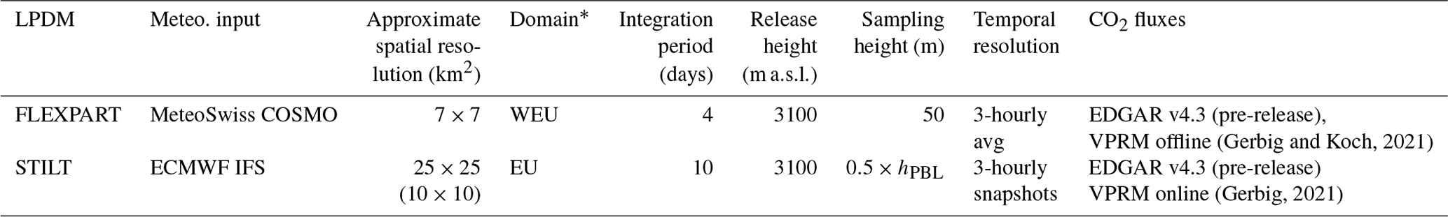
^* EU and WEU refer to 33^∘–73^∘ N, − 15–35^∘ E and 36.06–57.42^∘ N, −11.92–21.04^∘ E, respectively.

2.2.1 FLEXPART–COSMO

A version of the LPDM FLEXPART (Pisso et al., 2019; Stohl et al., 2005) coupled to output from the regional numerical weather prediction model COSMO (Baldauf et al., 2011) was operated using operational analysis fields generated by MeteoSwiss (see Henne et al., 2016). The model was run in backward mode to calculate source sensitivities for JFJ. Within each 3-hourly interval, 50 000 model particles were continuously initialized at the receptor location and traced back in time for 4 d or until they left the model domain. FLEXPART considers transport by the mean atmospheric flow as well as turbulent and sub-grid-scale convective mixing. COSMO analyses were available hourly at a horizontal resolution of approximately 7 km × 7 km over western Europe (COSMO-7; 36.06–57.42^∘ N, −11.92–21.04^∘ E; Fig. S1 in the Supplement). The horizontal resolution of the model does not resolve the steep topography around JFJ. Hence, a difference between observatory and model altitude exists. In previous studies (e.g. Keller et al., 2011), the optimal release height was determined to be around 3100 m a.s.l. when using COSMO-7 inputs, which is between the true altitude (3580 m) and the model topography (2650 m) at JFJ. Surface source sensitivities were determined from the location of model particles below a sampling height of 50 m and stored 3-hourly along the backward simulation, allowing for a 3-hourly coupling to temporally variable surface fluxes.

2.2.2 STILT-ECMWF

The Stochastic Time-Inverted Lagrangian Transport (STILT) model, first described by Lin et al. (2003), was driven by the numerical weather forecast fields from the European Centre for Medium-Range Weather Forecasts (ECMWF), as previously presented by Trusilova et al. (2010) and Kountouris et al. (2018a). The simulations for JFJ were performed at the same release height as with FLEXPART–COSMO (3100 m a.s.l.), corresponding to 960 m above the model topography. STILT-ECMWF simulations are also routinely performed within the activities of the ICOS Carbon Portal (CP), albeit at a release height of 720 m above model ground (2860 m a.s.l.) for the default products for JFJ (https://stilt.icos-cp.eu/worker/, last access: 12 May 2022, ICOS Carbon Portal, 2022). The particles are released instantly on a 3-hourly interval and traced back in time for 10 d or until they leave the European domain (33^∘–73^∘ N, 15^∘ W–35^∘ E; Fig. S1). The STILT calculations were driven by 3-hourly operational ECMWF-IFS analysis and forecast fields available at a resolution of 0.25^∘ × 0.25^∘ (approx. 25 km × 25 km), whereas STILT output was generated on a finer grid (approx. 10 km × 10 km). Surface source sensitivities were evaluated by using a variable sampling height (0.5 ×h_PBL); h_PBL is the PBL height diagnosed within STILT. Transport and fluxes were coupled at hourly time resolution.

2.3 CO₂ fluxes and boundary conditions for the atmospheric transport simulations

2.3.1 Regional CO₂

a. Anthropogenic emissions

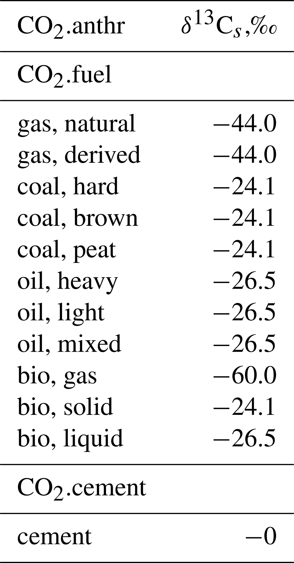
Regional anthropogenic CO₂ concentrations for JFJ (CO₂.anthr) were calculated using emission fluxes based on a pre-release of EDGAR v4.3 (G. Janssens-Maenhout, personal communication, 2013). The inventory was disaggregated into fuel-type-specific categories (Table S1) and provides annual emissions on a 0.1^∘ × 0.1^∘ grid (∼ 10 km × 10 km) (Janssens-Maenhout et al., 2019; Karstens, 2019). Here, we use 14 categories, representing 11 different fossil and biogenic fuel types as well as three non-fuel categories from cement and other production processes (Table 2). The CO₂.anthr comprises CO₂ from fuel-burning CO₂ (oil, gas, coal, liquid biofuels, biogas, solid biomass) and CO₂ from cement and other industrial production (referred to as CO₂.cement collectively). We temporally extrapolated the inventory, which was established for the base year 2010, using annual scaling factors per country and category based on data from BP (BP, 2019); see Table S2. Additionally, we applied seasonal, weekly, and diurnal time factors for different anthropogenic categories. These are based on MACC-TNO (Kuenen et al., 2014) and are available in Table S3.

Table 2 Fuel-type-specific δ¹³C_s assigned to the simulated anthropogenic CO₂ categories.

b. Ecosystem fluxes

Regional ecosystem CO₂ fluxes were based on the VPRM (Mahadevan et al., 2008). Underlying parameters are specific for seven vegetation types (VT) including (1) evergreen forest, (2) deciduous forest, (3) mixed forest, (4) shrubland, (5) savanna, (6) cropland, and (7) grassland. The VTs are based on the settings typically used within the ICOS Carbon Portal, although, for instance, category 5 (savanna) is irrelevant within the domain boundaries used for JFJ. An additional category, “others”, primarily includes water bodies and urban spaces for which VPRM does not estimate CO₂ fluxes and was hence excluded from the final analysis. The VT maps underlying VPRM are based on the synergetic land cover product (SYNMAP, Jung et al., 2006). A map showing the dominant category per grid as used in our study is provided in Fig. S2. Note that oceanic sources and sinks (including oceanic biomass), as well as human or animal respiration (see e.g. Ciais et al., 2020) and wildfire-related emissions, were not included and are expected to be a minor contribution to the regional signal at JFJ. With FLEXPART–COSMO, we use an offline version of VPRM (Gerbig and Koch, 2021) based on the same ECMWF meteorological analysis as in STILT-ECMWF. Although the fluxes are generated based on the individual VTs, ecosystem respiration (CO₂.resp), ecosystem uptake (also referred to as gross ecosystem exchange and thus abbreviated CO₂.gee), and net ecosystem exchange (CO₂.nee = CO₂.gee − CO₂.resp) are provided only as a total over all VTs. The STILT-ECMWF is coupled online with VPRM and allows extracting CO₂ concentration contributions at JFJ for CO₂.nee, CO₂.gee and CO₂.resp for the individual VTs separately. The online VPRM parameterization initially presented by Kountouris et al. (2018b) was updated for our study (Gerbig, 2021). A dedicated evaluation of the online and offline implementation with STILT-ECMWF for JFJ yielded comparable results for CO₂.nee, CO₂.gee, and CO₂.resp.

2.3.2 Background CO₂

We use the Jena CarboScope (JCS) global atmospheric CO₂ product for the determination of the CO₂ boundary conditions. These simulations are based on optimized fluxes (Rödenbeck, 2005) and are available at http://www.bgc-jena.mpg.de/CarboScope/ (last access: 12 May 2022, https://doi.org/10.17871/CarboScope-s04oc_v4.3). We used three-dimensional CarboScope fields (version or experiment: s04oc_v4.3) with a temporal resolution of 6 h and interpolated concentrations in space and time to the end points of model particles. The mean over all model particles of a given release forms the background concentration (denoted f_b herein) at the time of the release. We observed a higher short-term variability in the simulated background CO₂ concentration for FLEXPART–COSMO compared to STILT-ECMWF, which is a consequence of the smaller domain size, in particular towards eastern Europe, and shorter backward integration time (4 d versus 10 d).

2.3.3 Total CO₂

The sum of CO₂.anthr and CO₂.nee concentrations provides the regional contribution to the CO₂ concentration at JFJ (i.e. CO₂.regional). Together with the simulation-specific background for either FLEXPART–COSMO or STILT-ECMWF this yields the total CO₂ concentration (i.e. CO₂.total) at JFJ.

2.4 Model-based δ¹³C–CO₂ estimation

The stable carbon isotope ratio of CO₂ is referred to as δ¹³C–CO₂, or δ¹³C. The estimation of the mixed δ¹³C–CO₂ source signature (δ¹³C_m) and ambient δ¹³C–CO₂ isotope ratios (δ¹³C_a) is based on the CO₂ concentration simulations. All δ¹³C–CO₂ estimates are given in per mille (‰) relative to the Vienna Pee Dee Belemnite (VPDB) reference standard. Further information on stable isotope expressions and definitions is available in Coplen (2011).

2.4.1 Mixed source signature (δ¹³C_m)

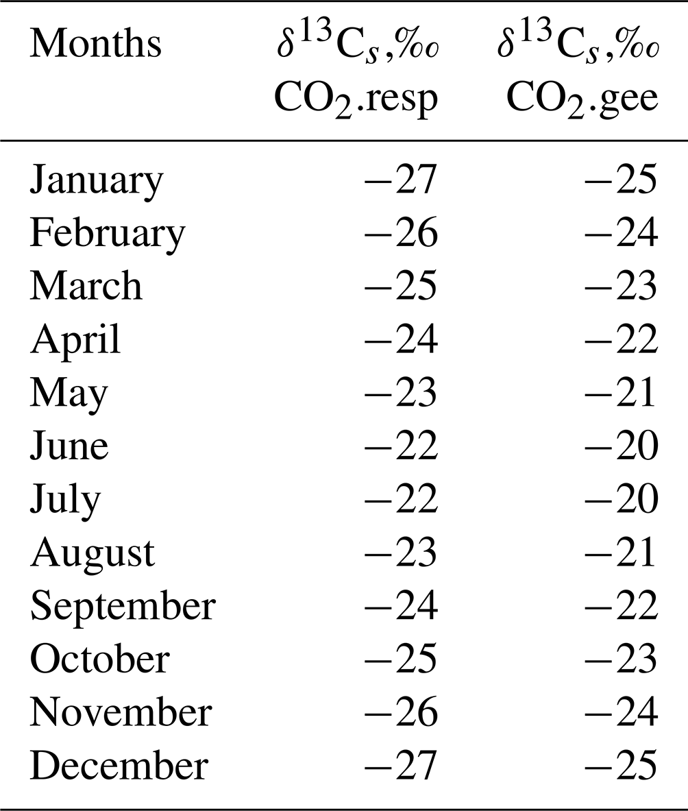
The absolute values of simulated CO₂ concentrations per source and sink category i, |f_s,i|, were weighted with category-specific source signatures, δ¹³C_s,i, to retrieve a mixed source signature, δ¹³C_m, according to Eq. (1) using the δ¹³C_s literature-based assumptions summarized in Tables 2 and 3. The simulated anthropogenic CO₂ data were disaggregated based on fuel type (Table 2) rather than sectorial processes because δ¹³C_s can best be attributed as a function of fuel type. For ecosystem fluxes, a seasonal cycle in δ¹³C_s was assumed (Table 3). Following the reasoning of Vardag et al. (2016), the CO₂.gee was treated as a source, i.e. its absolute value was considered, along with the δ¹³C_s, using a reversed sign in Eq. (1).

Table 3 Assumptions for ecosystem δ¹³C_s based on Ballantyne et al. (2010, 2011) and Vardag et al. (2016).

Assumptions for fossil and cement sources are based on Andres et al. (1994). Gaseous fuels are characterized by a large range (− 15 ‰ to − 85 ‰) as reviewed by Sherwood et al. (2017), with a mean of − 44 ‰. The biogas signature is based on measurements of δ¹³C–CH₄ released by cows, a biogas production plant, and wastewater treatment (Hoheisel et al., 2019; Levin et al., 1993). The values are in line with microbial δ¹³C–CH₄ reviewed by Sherwood et al. (2017). CO₂.cement includes industrial emissions from cement production (NMM) alongside two minor contributors (CHE, IRO), as detailed in Table S1.

$$\begin{array}{}\text{(1)}& {\mathit{\delta }}^{\mathrm{13}}{\mathrm{C}}_{\mathrm{m}}={\displaystyle \frac{\sum {}_{n=\mathrm{1}}^i\left(\mathrm{|}{f}_{s,i}\mathrm{|}\times {\mathit{\delta }}^{\mathrm{13}}{\mathrm{C}}_{s,i}\right)}{\sum {}_{n=\mathrm{1}}^i\left(\mathrm{|}{f}_{s,i}\mathrm{|}\right)}}\end{array}$$

2.4.2 δ¹³C–CO₂ background estimate (δ¹³C_b)

The Jena CarboScope (JCS) CO₂ background concentration simulation for JFJ serves as f_b. The δ¹³C–CO₂ background value, δ¹³C_b, is estimated thereof through scaling f_b by using a relationship between observations of CO₂ and δ¹³C–CO₂ in background air (flask samples as detailed in Sect. 2.6). The relationship is derived following the strategy of Vardag et al. (2016) by applying yearly linear regression fits between measurements of CO₂ and δ¹³C–CO₂ under free troposphere conditions at JFJ (method A). The obtained δ¹³C_b is provided in Fig. S3. In addition to method A we also obtained estimates for δ¹³C_b based on a moving linear regression over a 12-month window (method B). Alternatively, we tested the ratio of δ¹³C–CO₂ and CO₂ in background air as a scaling factor using monthly data averaged over 2009–2017 (method C) and daily ratios (method D). The daily ratios were obtained from QCLAS measurements at 05:00–06:00 (UTC + 1), as the early morning is considered to be the background condition for JFJ. Results are available in Fig. S4.

2.4.3 Atmospheric δ¹³C–CO₂ estimates (δ¹³C_a)

The mixed source signature, δ¹³C_m, derived in Eq. (1) was combined with the background estimates (f_b, δ¹³C_b) in order to derive estimates of atmospheric δ¹³C–CO₂ isotope ratios at JFJ, δ¹³C_a, following Eq. (2). Note that, contrary to Eq. (1), CO₂.gee is considered to be an effective sink in Eq. (2), which is further detailed in Vardag et al. (2016).

$$\begin{array}{}\text{(2)}& {\mathit{\delta }}^{\mathrm{13}}{\mathrm{C}}_a={\displaystyle \frac{(f_b\times {\mathit{\delta }}^{\mathrm{13}}{\mathrm{C}}_b)+(\sum {}_{n=\mathrm{1}}^i\left(f_{s,i}\right)\times {\mathit{\delta }}^{\mathrm{13}}{\mathrm{C}}_{\mathrm{m}})}{f_b+\sum {}_{n=\mathrm{1}}^i\left(f_{s,i}\right)}}\end{array}$$

2.5 Observation-based δ¹³C–CO₂ estimation

Observation-based mixed source signatures, δ¹³C_m, were derived using a moving Keeling-plot approach following the example of Vardag et al. (2016) and using JFJ-specific fitting and filtering criteria, as detailed in Sect. 3.2.3.

2.6 Observations

The CO₂ concentrations and δ¹³C–CO₂ isotope ratios were continuously measured at JFJ by quantum cascade laser absorption spectroscopy (QCLAS) during the period 2009–2017. The custom-built QCLAS instrument (Nelson et al., 2008; Tuzson et al., 2008a, b, 2011; Sturm et al., 2013) provides high-precision data for the three main CO₂ isotopologues (¹²C¹⁶O₂, ¹³C¹⁶O₂, and ¹²C¹⁶O¹⁸O), and therefore it allows simultaneous determination of the CO₂ concentration and the δ¹³C–CO₂ and δ¹⁸O–CO₂ values at 1 s time resolution. The CO₂ dry air mole fractions (µmol mol⁻¹) are reported in units of parts per million (ppm) on the World Meteorological Organization (WMO) CO₂ X2007 scale, while the isotope ratio values are given in per mille (‰) relative to the Vienna Pee Dee Belemnite (VPDB) reference standard. The instrument was configured as described in Tuzson et al. (2011) during 2009–2011. The hardware and calibration strategy were revised during an upgrade in 2012, as described in Sturm et al. (2013) to improve long-term precision, stability, and traceability within the International System of Units (SI). Furthermore, the instrument participated in the WMO/IAEA Round Robin 6 Comparison Experiment to assess the instrument capability to maintain the link to the WMO recommended level under field operation (NOAA, 2015). Stable operating conditions guarantee a precision of 0.02 ‰ for δ¹³C–CO₂ and 0.01 ppm for CO₂ at an optimum averaging time of 10 min. During 2016–2017, laboratory temperature instabilities adversely affected instrument performance, causing lower data coverage. CO₂ concentrations have additionally been determined at 1 min time resolution by a commercial cavity ring-down spectrometer (CRDS, G2401; Picarro Inc., USA) since 2010, likewise linked to the WMO CO₂ X2007 scale. These data are available as an ICOS product (Emmenegger et al., 2020). The mean difference (1σ) between the 1 min averaged CRDS and QCLAS data is 0.1 ± 0.4 ppm for the entire observation period. Besides the in situ measurements, air samples were collected in triplicate every second Friday at around 7:00 local time, i.e. at a time when the JFJ site predominantly experiences lower free troposphere conditions (Herrmann et al., 2015). CO₂ concentration, δ¹³C–CO₂, and δ¹⁸O–CO₂ in the flask samples were analysed at Max Planck Institute for Biogeochemistry (MPI-BGC) in Jena as described in Van Der Laan-Luijkx et al. (2013). The flask data, which defined by the sampling time correspond primarily to background conditions at JFJ, are used to construct δ¹³C_b. A comparison of flask sample measurements with the QCLAS measurements for 2009–2017 indicates very good agreement, typically within ± 0.2 ppm for CO₂ and ± 0.1 ‰ for δ¹³C–CO₂, as well as no apparent systematic bias as a function of time or signal intensity. It should be noted that the data and sample collection for in situ measurements (QCLAS) and offline samples (flasks) were not primarily designed to assess an intercomparison between the two measurement systems. In particular, uncertainties exist regarding the accurate matching of time stamps. Therefore, the real agreement of the measurements is likely even better.

2.7 Time series analysis

Time series analysis was performed using R programming language v3.6.1 (R Core Team, 2019) by deploying available R packages (https://cran.r-project.org, last access: 12 May 2022) as well as custom-developed scripts. While FLEXPART–COSMO simulations provide 3-hourly averages, STILT-ECMWF provides instantaneous snapshots every third hour. STILT-ECMWF simulations were interpolated between the 3-hourly nodes for comparison with 3-hourly averages of observational data. For comparing the observations with the LPDM output, we use 3-hourly and monthly averages of the QCLAS measurements. Furthermore, a common JCS-based background is subtracted from the measurements. The STILT-ECMWF JCS-based background is preferred as the common background for this particular assessment over the FLEXPART–COSMO background owing to the higher short-term variations in the latter (compare Fig. S3a). The background-subtracted data set is referred to as “regional observations”.

3 Results and discussion

3.1 Regional CO₂ simulations at JFJ

3.1.1 Monthly timescale

a. Planetary boundary layer influence at JFJ

Air mass transport dynamics determine the exposure of the receptor site JFJ to air masses from the planetary boundary layer (PBL). Thus, together with the source or sink strength in the footprint region, they drive the regional contributions to the CO₂ concentrations and are discussed up front. Previous analyses of tracers (e.g. radon and CO-to-NO_y ratio) by Herrmann et al. (2015) suggested that, compared to winter (December–February), the PBL influence at JFJ is enhanced by 1.5- to 2.5-fold in April and August–September and by 3 to 4-fold from May–July. To isolate the influence of seasonally varying transport, we performed dedicated simulations wherein CO₂ fluxes were assumed constant in space and time (see Appendix A1). This analysis revealed a 2- to 3-fold larger simulated PBL influence in summer compared to winter for both models. Diurnal variations were most pronounced in summer, indicating a 1.4-fold larger PBL influence during the afternoon and evening (maximum at ∼ 16:00, UTC + 1) compared to the morning (minimum at ∼ 10:00, UTC + 1). A larger PBL influence in May and September for STILT-ECMWF compared to FLEXPART–COSMO appears to be a peculiarity of using ECMWF fields and may reflect the less-well resolved transport in complex terrain in the coarser-resolution data from ECMWF. Additional differences appear to be related to the smaller domain size and shorter backward integration used for FLEXPART–COSMO, which are directly associated with smaller integrated surface CO₂ fluxes. The findings for STILT-ECMWF and FLEXPART–COSMO from the transport dynamics analysis (Appendix A1) appear to explain some of the mismatch in the simulated CO₂ observed between the simulations in Fig. 1 (see Sect. 3.1.1b).

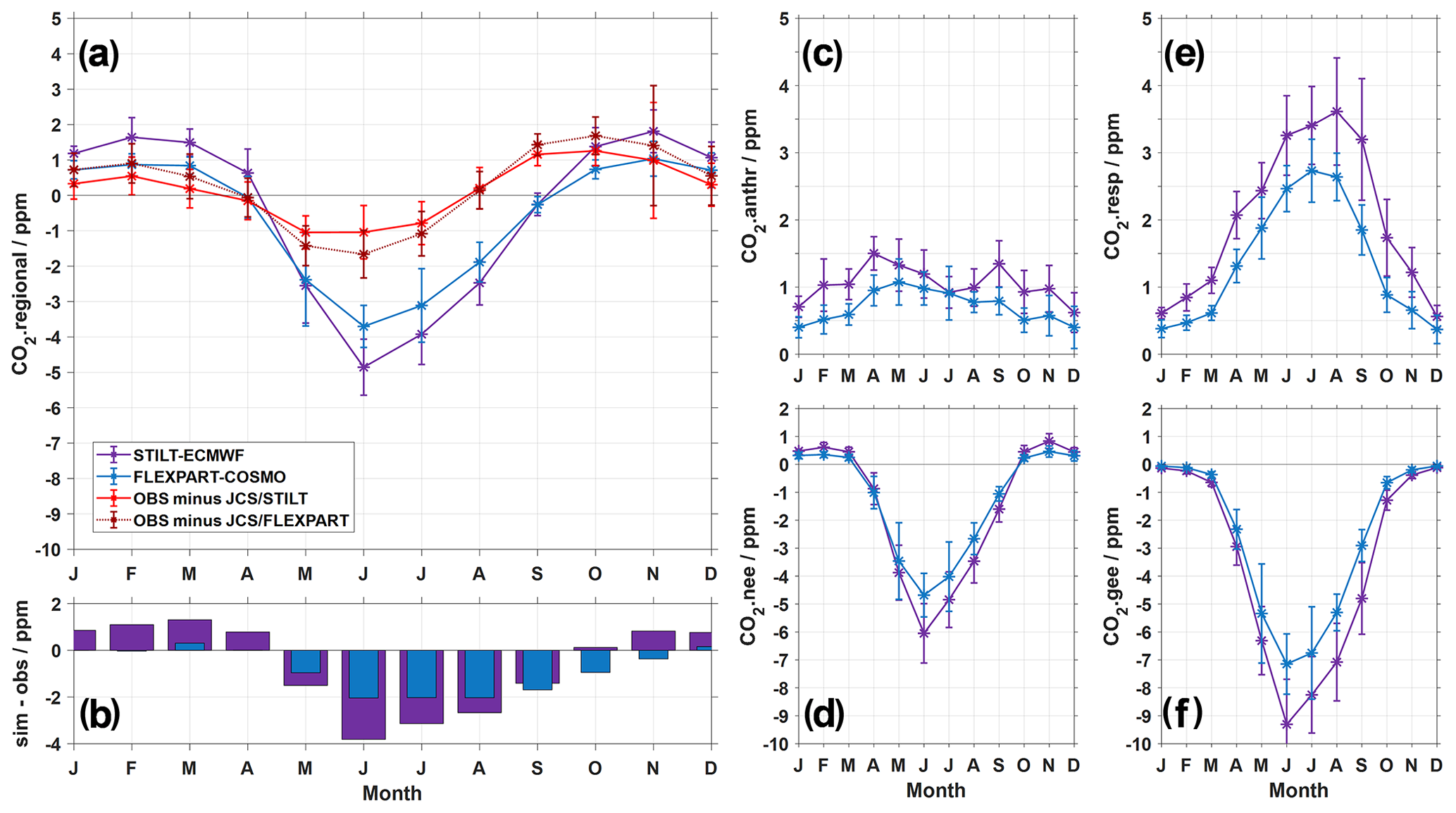
Figure 1 Multi-annual monthly means of 3-hourly regional CO₂ simulations compared to observations (2009–2017). CO₂.regional (a), its components CO₂.anthr (c), and net ecosystem exchange (CO₂.nee) (d). The difference between simulations (sim) and observations (obs) is presented in (b). CO₂.nee is composed of (e) gross ecosystem respiration (CO₂.resp) and (f) gross ecosystem exchange (CO₂.gee), i.e. gross uptake. Error bars represent 1 SD of the multi-annual means and reflect the year-to-year variability for 2009–2017.

b. Regional CO₂ concentration observations and simulations

Simulated CO₂.regional for 2009–2017 is compared with the respective regional CO₂ concentration observations in Fig. 1 (multi-annual monthly means). The CO₂.regional observations show a minimum in June and a maximum in October and November, both with an amplitude of about 1.8 ppm. Smaller panels present the corresponding simulated anthropogenic (CO₂.anthr) and ecosystem components (CO₂.nee, CO₂.gee, CO₂.resp).

While CO₂.anthr and CO₂.nee together constitute CO₂.regional, the sum of ecosystem components CO₂.gee and CO₂.resp results in CO₂.nee. The minimum in June as observed in the measurements is well represented by the models, though the amplitude is overestimated. The October–November maximum is delayed in both models by about 1 month. A local minimum in December–January is seen in observations and models. The winter minimum in the regional signal reflects the limited influence of PBL air masses at JFJ during this period of the year and coincides with a minimum in CO₂.anthr (Fig. 1c) and ecosystem CO₂ (Fig. 1d–f). The models thus appear to represent the processes contributing to the seasonal variability of the regional CO₂ signal at JFJ quite realistically. It is noteworthy that the seasonal trends of the regional signal, in particular the local winter minimum, differ from those in the large-scale CO₂ background concentrations, which show a minimum in August, 2 months later than the regional signal, and only one maximum in March–April, as shown by Sturm et al. (2013).

Regarding CO₂.anthr (Fig. 1c), we conclude that the reduced transport of PBL air to JFJ during December–January outweighs a maximum in anthropogenic surface emission fluxes related to enhanced fuel use for heating during the cold season. Instead, CO₂.anthr simulations reach a maximum at JFJ in spring (April–May) in both models, resulting from still relatively large anthropogenic surface emissions and generally more unstable atmospheric conditions due to rising surface temperatures and sustained colder temperatures aloft. The STILT-ECMWF simulations comprise a second CO₂.anthr maximum in autumn (September), which is in line with the simulated PBL influence (Appendix A1).

Given that ecosystem contributions quantitatively dominate the regional contributions to CO₂ concentrations during summer, we reiterate that the CO₂.nee simulations depend on the parameterization of ecosystem respiration and uptake fluxes in VPRM. The parameterization accounts for environmental factors such as temperature, radiation, and, through MODIS-derived enhanced vegetation index (EVI) and land surface water index (LSWI), also for soil moisture (Mahadevan et al., 2008). Warmer temperatures generally lead to enhanced gross ecosystem fluxes (CO₂.resp and CO₂.gee) in summer compared to winter. These trends are indeed reflected in the simulations for JFJ (Fig. 1d–f). The strong negative regional CO₂.nee from March to October is a result of only partial compensation of uptake (CO₂.gee) by respiration (CO₂.resp). The CO₂.gee minimum in June does not coincide with the CO₂.resp maximum in July–August. This may be explained by the fact that respiration is strongly dependent on temperature, and July and August typically show the highest average temperatures in the relevant footprint region. Ecosystem uptake, on the other hand, has a more complex relationship with temperature (drops off when too hot), radiation (actually largest in June), water availability (usually decreasing during the summer), and plant phenology (e.g. Bonan, 2015; Mahadevan et al., 2008).

The simulations qualitatively satisfy our expectations. However, the overestimation of the amplitude in summer and early autumn by the two models merits further discussion of potential contributions to this mismatch, which includes uncertainties in the transport model or in the spatio-temporal flux distribution. A quantitative assessment is available in Sect. 3.2.2c.

• 1.

  Transport dynamics. The fluxes computed by VPRM together with the air mass transport dynamics determine the final seasonality of the ecosystem-related CO₂ contributions at JFJ.

  • a.

    It has been reported by Denning et al. (1999) that the signal from respiration CO₂ is amplified over flat terrain because respiration dominates at night when the boundary layer is shallow. This observation is referred to as the rectifier effect. At JFJ, we likely observe the inverse situation, a fair-weather effect, as warm and sunny afternoons favour PBL influence at JFJ, while low-irradiation periods (nighttime, winter) limit the PBL influence. Vertical atmospheric transport and photosynthetic activity (uptake) covary and are both largest on sunny days. In contrast, ecosystem respiration is active independently of light condition (day–night) and, to a smaller degree, during colder periods, when PBL influence is limited at JFJ. Such fair-weather effects may be inadequately captured in the models, as the vertical export of PBL air in these situations is driven by thermally induced flow systems in complex terrain (up-slope, up-valley; see Rotach et al., 2014) that cannot be adequately resolved at the present model horizontal resolution.

  • b.

    The simulations for JFJ indicate that a considerable fraction of ecosystem CO₂ originated from fluxes within the last few hours before arrival at JFJ and at distances shorter than 100 km from the site (predominantly north of JFJ). We find that this “nearby” contribution is particularly pronounced in summer, whereas cold season sampled air masses are rather associated with a much wider concentration footprint and are less dominated by nearby vegetation fluxes. In addition, the nearby vegetation fluxes seem artificially enhanced by the limited spatial resolution of the vegetation maps.

• 2.

  VPRM. An overestimation of the CO₂.gee or an underestimation of CO₂.resp may be associated with harvesting activities and drought stress, which are not well reflected in the current parameterization of VPRM, as well as the spatial representation of vegetation maps and temperature profiles.

  • a.

    Harvesting usually results in a change in the enhanced vegetation index (EVI) derived from the MODIS observations. While the reduced ecosystem uptake due to harvesting is thus in principle already represented in VPRM, the agricultural biomass left behind after the harvest may lead to increased respiration. VPRM is unlikely to capture this latter process with its simple linear dependence of respiration on temperature.

  • b.

    Water stress (drought) can lead to altered respiration and uptake fluxes (e.g. Ramonet et al., 2020, or Gharun et al., 2020), but it is not explicitly included in VPRM.

  • c.

    Owing to the smoothed topography and vegetation maps in the models, the effective temperatures in Alpine vegetation are likely not well represented, and, moreover, the temperature parameterizations in VPRM are not optimized for Alpine vegetation. No systematic bias net ecosystem exchange is apparent for ecosystem simulations with STILT-ECMWF for other observational sites in Europe (data available at the ICOS Carbon Portal, 2022), suggesting that the discrepancy is predominantly linked to JFJ's location in complex terrain. Indeed, summer discrepancies appear to be comparatively large at JFJ (3580 m a.s.l.) even when considering other mountain stations, such as Monte Cimone (∼ 2000 m a.s.l., Italy) or Puy de Dôme (∼ 1500 m a.s.l., France), which are characterized by lower altitude and less complex topography compared to JFJ.

  Uncertainties in daily ecosystem fluxes are estimated in Kountouris et al. (2015), based on a comparison with eddy covariance flux observations, to be 2.5 µmol m⁻² s⁻¹ for VPRM, with typical spatial error correlation of around 100 km and a temporal correlation of 30 d. To estimate the impact of this uncertainty between eddy covariance data and simulations using VPRM on the simulated CO₂, however, full propagation of the error would be required, including spatial and temporal correlation. As VPRM is used in many inversion studies, the corresponding error in simulated CO₂ can alternatively be assessed based on the change from prior to posterior model–data mismatch. Based on Table 3 in the Technical Note of Kountouris et al. (2018b), typical numbers for mountain sites such as JFJ are around 4 ppm (prior), which drop to about 1.5 ppm for posterior fluxes (the assumed model–data mismatch error).

• 3.

  EDGAR. A mismatch between CO₂.regional simulations and observations may also result from biases in the CO₂.anthr signal. However, as quantified in Sect. 3.2.2c, an increase in CO₂.anthr by a factor of 3 to 4 would be required in order to compensate for the summer mismatch. Further, the discrepancy during summer is much larger than that during winter when CO₂.anthr contributes the largest share, and we consider it thus unlikely that CO₂.anthr is the main driver of the summer mismatch. As JFJ is also a popular destination for touristic day trips, local emissions from tourists and the JFJ infrastructure itself cannot be excluded. The recent study by Affolter et al. (2021), however, showed that this effect is expected to be well below the discrepancy between observations and simulations found here.

c. Composition of simulated anthropogenic and ecosystem CO₂

Ecosystem contributions to CO₂ concentrations outweigh the anthropogenic ones at JFJ most of the year if we consider the multi-annual monthly means (Fig. 1). For instance, gross respiration contributions to CO₂ concentrations are at their maximum 3–4-fold the anthropogenic ones during summer. However, gross respiration is overcompensated for by an up to 2-fold gross uptake in summer. During the colder period, gross respiration dominates the net ecosystem exchange and equals roughly the amounts of anthropogenic CO₂. While on a global scale monthly ecosystem fluxes indeed outweigh anthropogenic CO₂, this is not the case for urban areas. For instance, Vardag et al. (2016) suggest that on cold winter days, the CO₂ share in an urban environment in Germany (Heidelberg) is 90 %–95 % fuel-related, which is 2-fold the CO₂.anthr fraction compared to JFJ. Nevertheless, also in Heidelberg ecosystem contributions can make up 80 % in summer, similar to our simulations for JFJ.

In Fig. 2a and b we present the ecosystem contributions at JFJ split for the considered vegetation types (multi-annual monthly means for 2009–2017, available for STILT-ECMWF only). For summer, the largest fractions of simulated CO₂.resp are related to cropland (∼ 50 %), followed by forest (∼ 30 %) and grassland (∼ 10 %). During winter, the cropland share increases, while the mixed forest share decreases. This may be a result of the above-discussed change of footprint area from regional (cropland) in winter to more local (mixed forests) in summer. For CO₂.gee, it is important to consider that absolute quantities approach zero during the cold season and relative fractions are most meaningful in summer. The CO₂.gee generally displays a larger forest share in comparison to the one of CO₂.resp, possibly as air masses travel through forest-rich vegetated areas during the last few hours before reaching JFJ (which corresponds to daytime, when uptake is active). Furthermore, we observe a shift in the relative CO₂.gee share from cropland to forest from April to September, which is likely the result of vegetation dynamics, considering that crops mature earlier in the year, and forests absorb carbon much longer during the growing season.

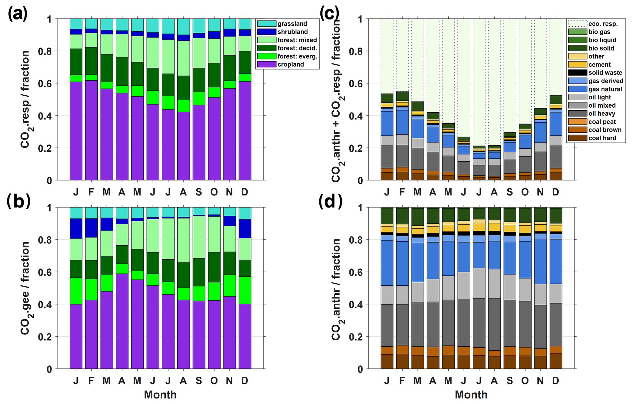
Figure 2 Simulated regional contributions to the CO₂ concentrations at JFJ (multi-annual monthly means of 3-hourly simulations, 2009–2017, STILT-ECMWF). (a) Gross ecosystem respiration per vegetation type (CO₂.resp), (b) gross ecosystem exchange (uptake) per vegetation type (CO₂.gee), (c) CO₂.anthr and CO₂.resp, (d) CO₂.anthr per fuel-type. Maps of anthropogenic fluxes and vegetation distribution are provided in Figs. S1 and S2.

In Fig. 2c and d we present the relative fractions of CO₂.anthr. The contributions associated with fossil sources sum up to 90 % of CO₂.anthr. The CO₂.anthr is dominated by CO₂ from liquid fuel use, in particular light and heavy oil used for on- and off-road transport as well as domestic heating (∼ 50 %). A further 25 % of CO₂.anthr is related to natural gas, and only 10 % is attributed to solid fossil fuels, including a larger fraction of hard coal and a smaller fraction of brown coal. Solid biomass, such as residential wood burning for domestic heating, contributes 10 % to CO₂.anthr. Non-combustion CO₂ from cement and other industry production amounts to 5 % of CO₂.anthr at JFJ. Seasonal shifts are observed in the contribution of solid biomass (higher in winter, lower in summer) as well as in relative fractions of light oil (higher in summer) and natural gas (lower in summer). The relative contributions of FLEXPART–COSMO (not shown here) are very similar to the ones of STILT-ECMWF despite the differences in the absolute quantities of CO₂.anthr between the two models (Fig. 1), which, as discussed above, are primarily driven by the model's implementation of transport dynamics.

3.1.2 Regression analysis of hourly-scale CO₂ simulations vs. observations

The model performance was further evaluated by comparing the 3-hourly simulated CO₂ concentration time series with observations. In Fig. 3 we present CO₂.total, which includes background (f_b) and regional contributions (CO₂.regional, i.e. the sum of f_s,i). In order to derive CO₂.total, the simulation-specific background (i.e. either FLEXPART–COSMO or STILT-ECMWF) was added to the respective CO₂.regional data. Overall, the simulations capture the intensity and timing of individual regional short-term events at the models' 3-hourly time resolution to a high degree, in addition to the good representation of annual and seasonal trends.

Figure 3 Time series of CO₂.total simulations with (a, c) FLEXPART–COSMO and (b, d) STILT-ECMWF compared to hourly observations. (a, b) 2009–2017 (tick marks indicate January of each year), (c, d) 2013 (JCS-based background is detailed in Fig. S3a).

We assess the performance separately for the four seasons winter (December–February, or DJF), spring (March–May, or MAM), summer (June–August, or JJA), and autumn (September–November, or SON) for the CO₂.regional signal, as summarized in Fig. 4, and show a 4-year subset for 2012–2015 in addition to the full 9-year observation period (2009–2017). The subset is of interest as it comprises a higher frequency and intensity of regional CO₂ at JFJ, in particular considering the winter of 2012/2013, and in addition, measurements by QCLAS had the best performance during 2012–2015. We primarily consider the coefficient of determination, r², regression slope, and bias-corrected root mean square error (BRMS) in the assessment of the short-term variability.

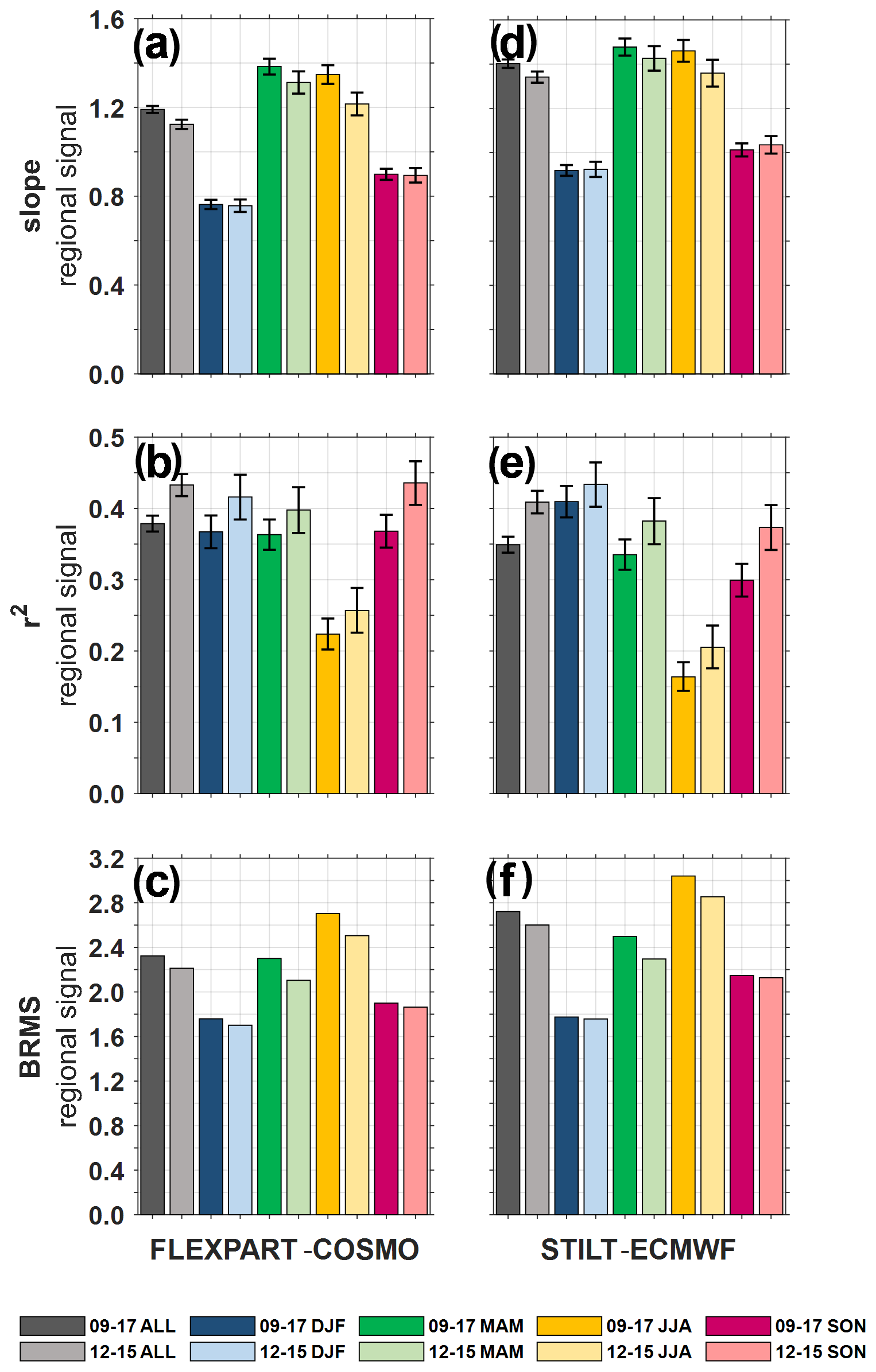
Figure 4 Summary of the regression analysis of CO₂.regional simulations vs. observation (data are based on 3-hourly time resolution; error bars show the 95 % confidence interval). The parameters (slope, r² and bias-corrected RMSE, i.e. BRMS) are presented for FLEXPART–COSMO (a–c) and STILT-ECMWF (d–f), including the full observation period, 2009–2017, and a 4-year subset (2012–2015).

The mean bias (labelled Y–X) provided in Fig. 5 is usually smaller than 1 ppm with the exception of summer, when the models exhibit a negative bias of up to 2.5 ppm. Removing this bias before calculating the root mean square error (RMSE) focuses on the short-term variability. The BRMS ranges from 1.8 to 3.1 ppm CO₂, with the lowest errors observed during winter and autumn and the highest errors in summer. For the 3-hourly data, both models reproduce the regional signal with similar quality. The r² is 0.44 for FLEXPART–COSMO and 0.41 for STILT-ECMWF, meaning that the models explain about 40 % of the observed regional CO₂ variability at JFJ. Considering the complex topography and small amplitude of the regional signal, this is a very satisfactory result and is in line with comparable simulations by Henne et al. (2016), which were able to explain a similar fraction of variability in regional CH₄ at JFJ for the year 2012 after simulation optimization with respect to CH₄ emissions.

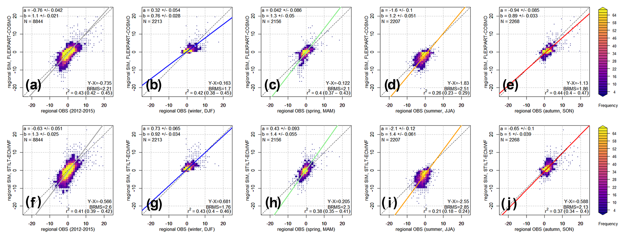
Figure 5 Heat maps for CO₂.regional simulations (SIM) using FLEXPART–COSMO (a–e) and STILT-ECMWF (f–j) in comparison to regional components of observations (OBS) for 2012–2015 (full year and per season) at 3-hourly time resolution. The STILT-ECMWF-based JCS background is subtracted from the observations to derive the regional component. The weighted least squares regression takes into account uncertainties in both data sets (the full-page version of this figure is available in the Supplement).

When analysing individual seasons, we find that the summer period is characterized by significantly lower r² for the 3-hourly data compared to the other seasons, although, aside from the above-mentioned negative bias, diurnal profiles in the observations during summer are well represented by the simulations. The slightly better performance for FLEXPART–COSMO compared to STILT-ECMWF in terms of mean bias and r² for 3-hourly data may be partly attributed to the higher spatial resolution that potentially allows for a better representation of thermally driven atmospheric transport in mountainous terrain during summer. Note that when adding model-specific JCS background values to the regional simulations, r² values are substantially higher (∼ 0.6–0.9, not shown) because a considerable part of variability in CO₂.total derives from seasonal variability and long-term trends.

The regression slopes represent the factors by which simulation and observation intensities agree with each other. For CO₂.regional, the intensity agreement (slope, ∼ 0.9–1.5) varies as a function of season and model. Slopes are closest to 1 in autumn–winter, and, as for other regression parameters, larger discrepancies occur in spring–summer. The spring–summer discrepancies are driven by negative excursions from the baseline in analogy to the larger warm season mismatch (discussed in Sect. 3.1.1) and higher mean bias. Again, note that we find the slopes for CO₂.total to be closer to 1 (∼ 0.9–1.3, not shown) than those for the CO₂.regional, confirming the appropriate assumptions for the background CO₂ concentrations.

3.2 Atmospheric δ¹³C–CO₂

Simulating regional signals at a high Alpine background site like JFJ is challenging, yet JFJ is one of very few stations that offer continuous high-frequency δ¹³C–CO₂ observations over multiple years. Thus, JFJ uniquely allows for combining model-based estimates of atmospheric δ¹³C–CO₂ and mixed source signatures (δ¹³C_m) with atmospheric δ¹³C–CO₂ observations and (“observation-based”) δ¹³C_m values derived thereof using a moving Keeling-plot approach.

3.2.1 Atmospheric δ¹³C–CO₂ estimates vs. observations

We evaluated the atmospheric δ¹³C–CO₂ isotope ratio estimates (δ¹³C_a), which are derived following Eq. (2) on a 3-hourly basis, through comparison with the QCLAS observations during the period 2012–2015 (Fig. 6, Table 4). Multi-annual monthly means for 2012–2015 are presented in Fig. 7.

Table 4 Summary of statistics on atmospheric δ¹³C–CO₂ estimates and observations for the period 2012–2015. Values for min, max, median (P₅₀), 25th and 75th percentiles (P₂₅ and P₇₅), mean (avg), and 1 SD are provided (hourly data) (see also Fig. S6).

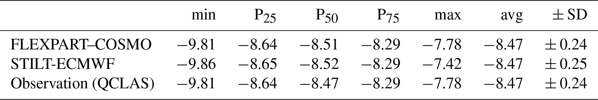
Figure 6 Time series of model-based and observed atmospheric δ¹³C–CO₂ for the years 2012–2015 (hourly observations). (a) FLEXPART–COSMO, (b) STILT-ECMWF; tick marks indicate January of each year. The background, δ¹³C_b, is presented in further detail in the Supplement (Fig. S3b). Data are presented at hourly time resolution (zoomed versions of this figure for 2012, 2013, 2014, and 2015 are provided in the Supplement; see Figs. S7–S9).

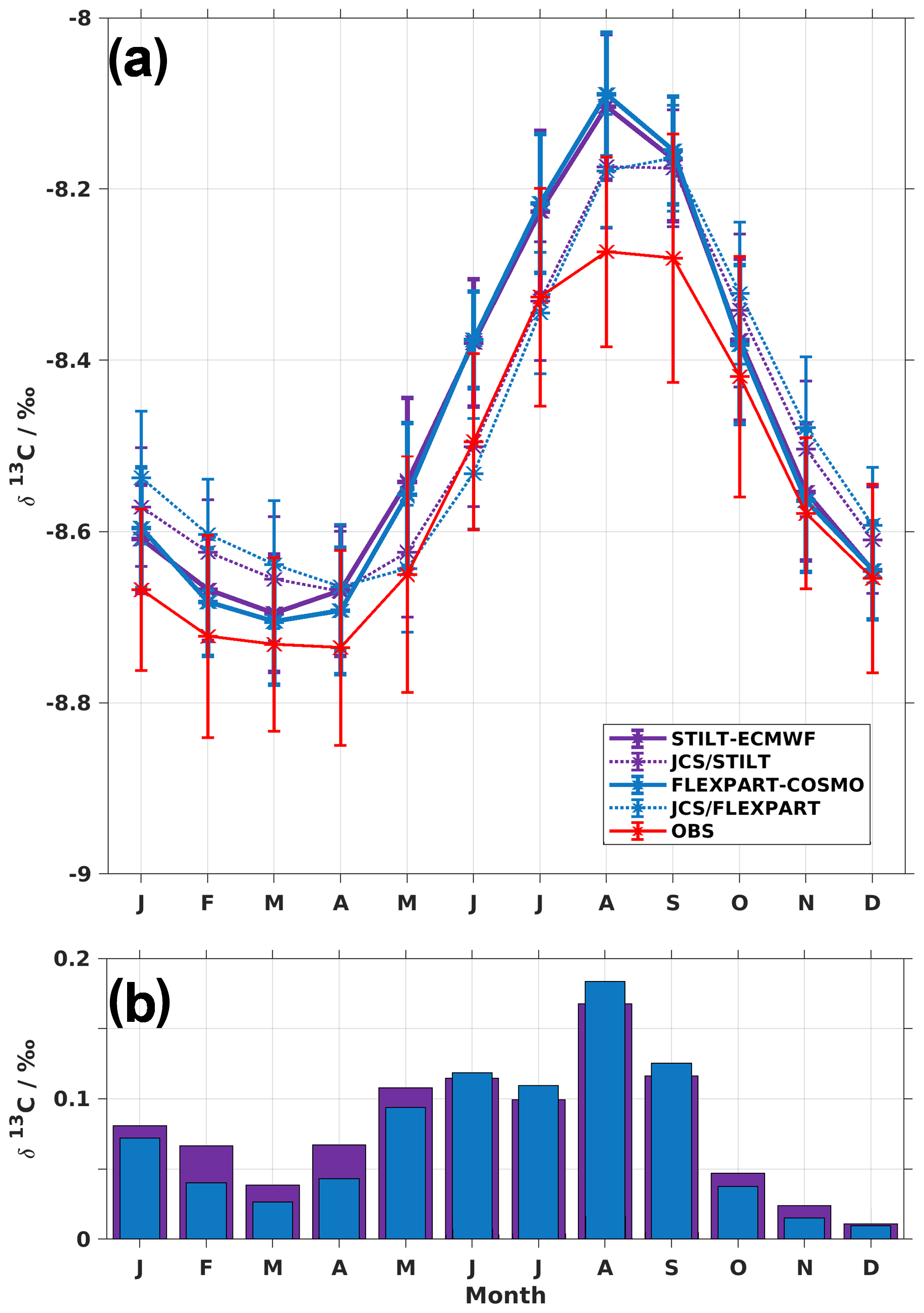
Figure 7 (a) Multi-annual monthly means of 3-hourly model-based and observed atmospheric δ¹³C–CO₂ for the years 2012–2015. Error bars represent 1 SD of the multi-annual means and reflect the year-to-year variability for 2012–2015. (b) Difference between simulations (sim) and observations (obs).

The simulated δ¹³C_a time series capture the observed variability in δ¹³C–CO₂ at JFJ well, in particular during the transition periods in spring and autumn. For most of the summer, however, the δ¹³C–CO₂ simulations are isotopically heavier than the observations; i.e. they appear more enriched in ¹³C. Despite an offset of ∼ 0.15 ‰, which appears to be related to the background (δ¹³C_b) assumptions, the diurnal profiles in the observations during summer are well represented by the simulations. Generally, the discrepancy in δ¹³C appears to be larger for STILT-ECMWF compared to FLEXPART–COSMO, and thus the discrepancy in CO₂ concentrations itself likely contributes to the mismatch in δ¹³C–CO₂, as further assessed in Sect. 3.2.2c–d, aside from uncertainties associated with assumptions for δ¹³C_s (discussed in Sect. 3.2.2a) and δ¹³C_b (Sect. 3.2.2b).

3.2.2 Sensitivity of δ¹³C–CO₂ estimates to different model assumptions

a. δ¹³C_s assumptions

The mixed source signature estimates (δ¹³C_m) as derived in Eq. (1) are presented in Fig. 8 on a 3-hourly timescale (monthly data are provided in Fig. S5). The estimated average δ¹³C_m is around − 24 ‰ and varies seasonally between around − 22 ‰ in summer and − 28 ‰ in winter for both FLEXPART–COSMO and STILT-ECMWF. Extreme values during particular events at 3-hourly time resolution reach − 35 ‰ when they are heavily impacted by anthropogenic fuel emissions, including a larger fraction of natural gas (∼ 50 % of regional CO₂), and values between − 17 ‰ and − 12 ‰ when impacted by cement production (∼ 30%). The δ¹³C_s from cement production originates from carbonates, which are characterized by a similar isotope composition as the carbonaceous VPDB reference material itself. Consequently, the δ¹³C_s for cement-related CO₂ is 0 ‰. Although cement-related CO₂ contributions to CO₂.regional at JFJ are about 1 order of magnitude smaller than from fuel burning or ecosystem processes, the influence of cement on δ¹³C_m is clearly visible in the model-based data in Fig. 8. These cement-related peaks in δ¹³C_m are, however, absent in δ¹³C_a (Fig. 6), simply because even the most intense cement signals at around 1–2 ppm are much smaller than other CO₂ contributions. Thus, when mixed with the background, the signal is diluted.

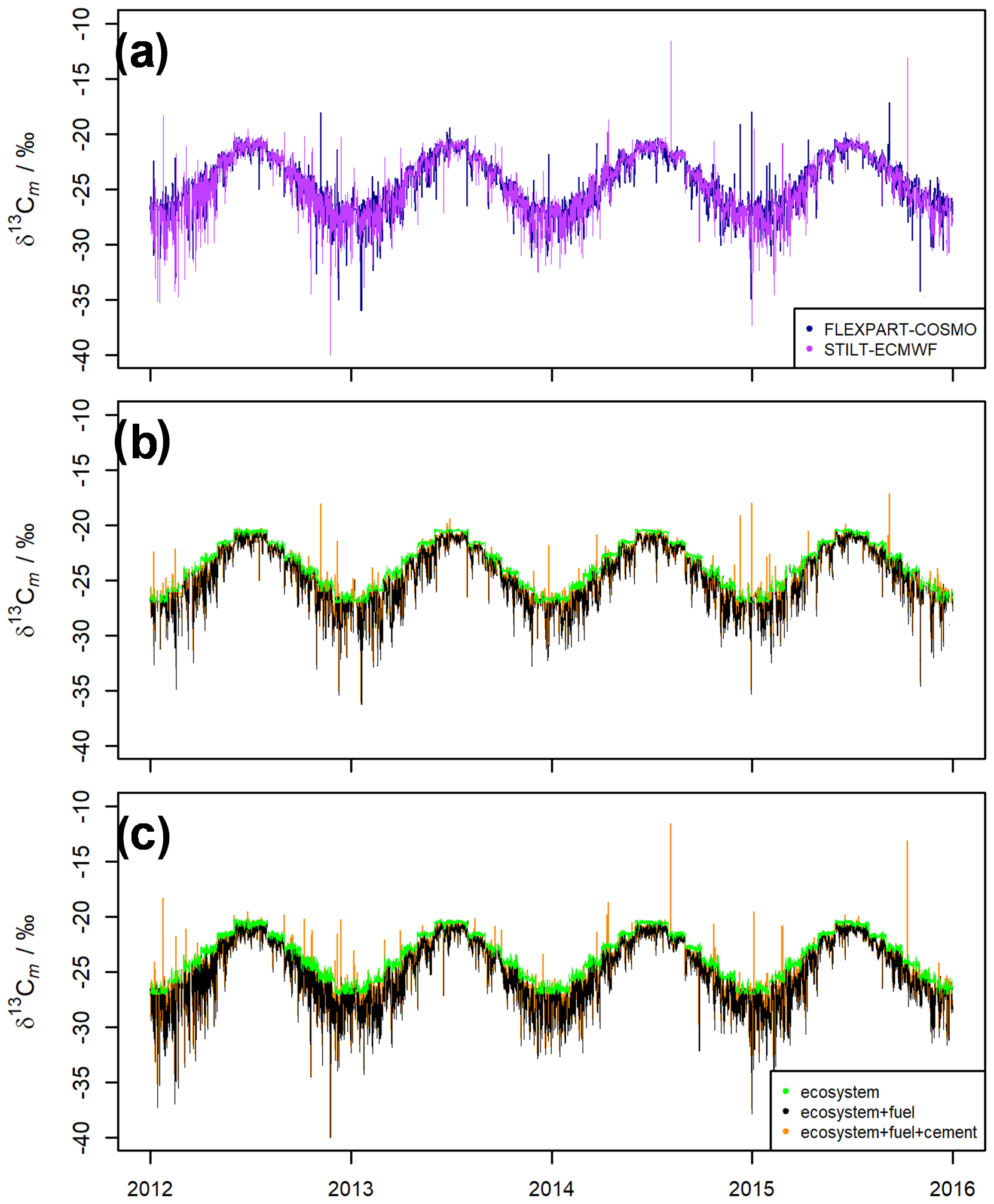
Figure 8 Time series of (a) model-based δ¹³C_m (Eq. 1) and (b–c) model-based δ¹³C_m for ecosystem-, fuel-, and cement-related CO₂: (b) FLEXPART–COSMO, (c) STILT-ECMWF; hourly data are used; tick marks indicate January of each year (see also Fig. S5).

The δ¹³C_s values, which are underlying the δ¹³C_m, represent the best available information in the scientific literature. However, while we use static assumptions, these values may vary in reality with air mass source region (footprint) and over time. Further uncertainties may arise from assumed ecosystem δ¹³C_s. For instance, C₄ plants are not explicitly represented in our model as a dedicated vegetation type with known spatial distribution. Yet, their contribution to average ecosystem δ¹³C_s is captured in the data of Ballantyne et al. (2010, 2011), which are underlying the assumptions in Table 3, as these are derived from ambient measurements in mixed C₃–C₄ ecosystems representative for the Northern Hemisphere. In the footprint region of JFJ, C₄ plants are mainly present in cropland due to maize production. For the year 2017, EUROSTAT reports that grain maize production made up around 21 % of the overall grain and cereal production by weight within the EU-28. Of all cropland, roughly 35 % on a land surface basis is assigned to grain and cereals. Applying a simple “back-of-the-envelope” calculation, this equates to ∼ 7 % of C₄-related CO₂ fluxes within the European Union as a yearly average. Because maize production is primarily relevant during the spring and summer, the fraction would be enhanced for this period of the year. Replacing 7 % of the C₃-related CO₂ with C₄-related CO₂ would marginally change the source signature of crops (< 1 ‰, and that of the overall ecosystem signal by even less); however, generally δ¹³C_m would become more enriched and thus the discrepancy between models and observations larger. Reducing a potential C₄-related CO₂ fraction instead would make δ¹³C_m less enriched and thus bring the simulation data into slightly better agreement with observations at JFJ. Indeed, the ecosystem assumptions for the Northern Hemisphere are based on data collected in the USA and might be characterized by a higher C₄ fraction than the footprint region for JFJ.

Vardag et al. (2016) report a measurement-based mean source signature (δ¹³C_m) of − 26 ‰ in summer and about − 32 ‰ in winter for Heidelberg, which is isotopically lighter when compared to the simulated δ¹³C_m for JFJ (− 22 ‰ in summer, − 28 ‰ in winter). The winter differences between Heidelberg and JFJ are reasonable as they may derive from larger ecosystem contributions at JFJ (50 %) compared to Heidelberg (5 %). The summer differences, however, may, aside from summer overestimations of CO₂.regional at JFJ, result from uncertainties in the assumption for the ecosystem δ¹³C_s including the uncertainty of the C₄-related CO₂ fraction. Indeed, Vardag et al. (2016) also suggest that the assumption of δ¹³C${}_s=-$ 23 ‰ for ecosystem CO₂ by Ballantyne et al. (2011) is too enriched for August and September in Heidelberg, and a more depleted assumption (through adjusting the seasonality in δ¹³C_s) would result in improved agreement between model-based δ¹³C–CO₂ and observations at JFJ.

b. δ¹³C_b assumptions

The background (δ¹³C_b; see Figs. 6, 7, and the Supplement), as estimated by the baseline CO₂ taken from the JCS assimilation system and the empirical δ¹³C–CO₂ relationship based on yearly linear regression fits (method A), closely tracks the evolution of the observed δ¹³C–CO₂ values outside the peaks and varies seasonally. Yet, inconsistencies are apparent from the use of the yearly regression fits. Assuming a more depleted δ¹³C_b during the second half of the year, for instance by − 0.15 ‰ during late summer (August) and early autumn (September), and assuming a more enriched δ¹³C_b during the first half of the year, for instance by +0.05 ‰ to +0.10 ‰ from January to March, would reduce the discrepancies between observations and simulations. Indeed, the moving fit (method B, see Fig. S4b) improves the transitioning between years. However, the use of multi-annual monthly ratios in method C introduces discontinuities when transitioning between months, and the daily ratios (method D) introduce higher scatter and data gaps (see Fig. S4c–d).

c. Sensitivity to CO₂ concentrations

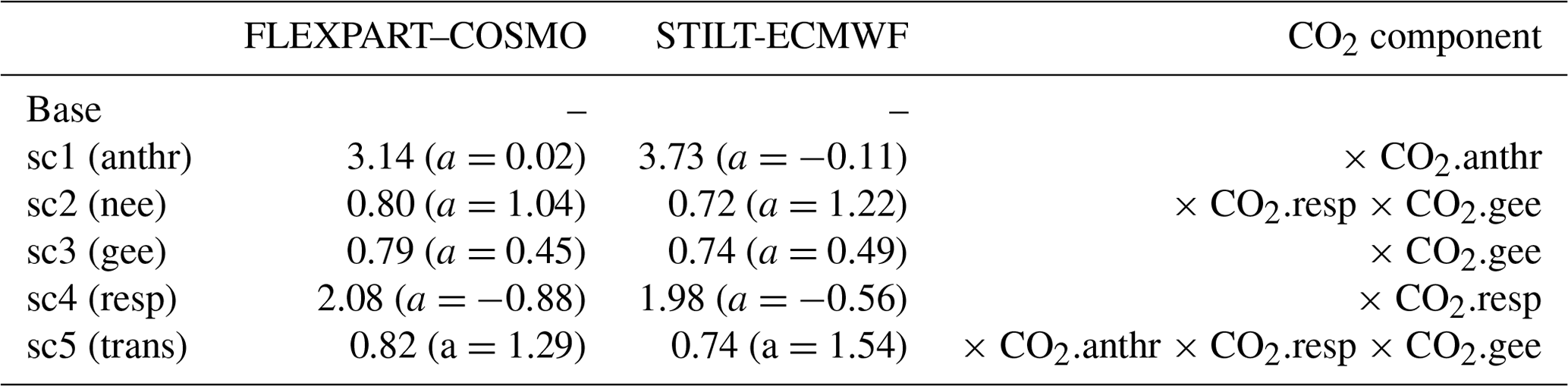
Based on the discussion in Sect. 3.1.1 we defined five scenarios, which aim to bring the simulated summertime CO₂.regional concentrations into better agreement with the observations. In each scenario, we adjust one or a combination of CO₂ sources and sinks by a single scaling factor for the whole summer period (JJA) for the years 2012–2015, thereby removing the model bias.

• Scenario 1 (sc1): through increasing CO₂.anthr we simulate a bias in the anthropogenic emission fluxes or a wrong seasonal factor for CO₂.anthr during summer.

• Scenario 2 (sc2): through reducing both CO₂.resp and CO₂.gee we attempt to represent a general VPRM parameterization or vegetation map representation issue.

• Scenario 3 (sc3): through reducing CO₂.gee we consider its potential overestimation by general VPRM parameterization or vegetation map representation issue in analogy to sc2; this is specific only to CO₂.gee.

• Scenario 4 (sc4): through increasing CO₂.resp we consider its potential overestimation by general VPRM parameterization or vegetation map representation issue in analogy to sc2; this is specific only to CO₂.resp.

• Scenario 5 (sc5): through modifying all signals at equal amounts (CO₂.anthr, CO₂.resp, CO₂.gee) we attempt to represent a pure transport issue (i.e. overrepresentation of PBL influence).

Scaling factors for each scenario were derived by weighted least squares regression and are presented in Table 5. The largest scaling factors of ∼ 3–4 are found for CO₂.anthr, followed by CO₂.resp (∼ 2), indicating that CO₂.anthr or CO₂.resp would need to be substantially increased in order to reduce the bias between models and observations. Instead, a reduction (scaling factor ∼ 0.7–0.8) would be required if only CO₂.gee was considered, and likewise a reduction in both CO₂.resp and CO₂.gee (scaling factor ∼ 0.7–0.8) in order to achieve a reduced CO₂.nee would lead to a reduced bias between the model and observations.

Table 5 Scaling factors based on the weighted least squares regression fitting slope b and intercept a (in parenthesis) used to minimize the CO₂ model bias for JJA (2012–2015).

d. Regression analysis for hourly δ¹³C–CO₂

We further evaluate the effect of CO₂ adjustments (Table 5) on the estimated regional δ¹³C–CO₂ at JFJ in comparison to the observations. First, however, we discuss the regression analysis for the base scenario. To obtain an estimate for regional δ¹³C–CO₂ a δ¹³C–CO₂ background needs to be subtracted from the total signal. Here, we used background method A, following the strategy used previously by Vardag et al. (2016). A higher short-term variability was observed for the δ¹³C_b from FLEXPART–COSMO compared to STILT-ECMWF (Fig. S3b). Consequently we used only the STILT-ECMWF-based δ¹³C_b for further calculations of regional components (i.e. for the subtraction of background values from the total signal).

Based on this particular δ¹³C_b assumption, the regional estimates agree with the regional observation intensity within a factor of 0.7–1, depending on season. The BRMS is between 0.12 ‰ and 0.14 ‰. Similar to CO₂, for spring, autumn, and winter the models capture the short-term variability in δ¹³C–CO₂ better than in summer. Overall, the r² values are lower than for CO₂ (max r²= 0.35 for FLEXPART–COSMO and 0.28 for STILT-ECMWF compared to about 0.4 for CO₂), which is not surprising given the uncertainties in the measurements as well as in the simulations, wherein, for instance, fixed source signatures were assumed. Despite the fact that model-based δ¹³C–CO₂ includes uncertainties of CO₂ simulation (used to construct δ¹³C_m), δ¹³C_s, and δ¹³C_b, the relative performance decreased by only 20 %–30 %. These results at JFJ were achieved with very low regional CO₂ signals, which, compared to the background (ΔCO₂), reached at maximum 30 ppm. Instead, the previously conducted urban studies benefitted from much more pronounced ΔCO₂ reaching up to ∼ 150 ppm for both Heidelberg (Vardag et al., 2016) and Downsview (Pugliese-Domenikos et al., 2019). However, they were limited regarding the length of the observation period (a few months in Downsview) and/or the stringent data filtering (e.g. Vardag et al., 2016, discarded 85 % of the data and biased the urban data sets towards nighttime observations, and Pugliese-Domenikos et al., 2019, discarded 80 % of the data for their isotopic mass balance approach). In contrast, the tall-tower study in rural England was challenged by a low signal-to-background ratio (ΔCO₂ reaching around 20 ppm), and isotope measurements were performed at low (weekly) time resolution, although simulations are provided on an hourly scale (Wenger et al., 2019). In comparison to the results from JFJ, Pugliese-Domenikos et al. (2019) reported an r=0.58 (r²=0.3), a root mean square error (RMSE) of 1.05 ‰, and a mean bias of 0.04 ‰ for a single month (January) for δ¹³C–CO₂. Wenger et al. (2019) do not provide any regression parameters for their model–observation comparisons; however, they observed large uncertainties in the δ¹³C–CO₂ estimation using a Monte Carlo approach. They related a part of their uncertainty for the δ¹³C–CO₂ estimates to the influence of ecosystem processes and the dominance of ecosystem fluxes in the regional CO₂ observations and simulations at the rural tall-tower site. Overall, the JFJ results are very well in line with previous findings despite the more remote location and correspondingly smaller magnitudes of regional signals at JFJ.

A representative set of results of the regression analysis for further scenarios as defined in Sect. 3.2.2c is summarized in the Supplement in Table S4. Overall, we find that modifications in sc 1 (CO₂.anthr) do not lead to improvement in the agreement between regional δ¹³C–CO₂ observations and simulations at 3-hourly resolution. Sc 5 (transport) results only in small improvements with regards to the BRMS. While the other scenarios do not result in major adjustments, for sc 3 (CO₂.gee) and sc 4 (CO₂.resp) we observe small model improvements with slightly increased r², slightly reduced BRMS, and a smaller bias (Y–X). Note that the remaining bias depends on the fitting intercept assumptions of the scaling factor. These results indicate that the δ¹³C simulation can be influenced through reasonable modification of CO₂ contributions. Discrepancies between observed and simulated δ¹³C–CO₂ are thus not exclusively related to uncertainties in source signature (δ¹³C_s) or background (δ¹³C_b) assumptions. However, an optimization of δ¹³C_b mentioned in Sect. 3.2.2b might result in improved agreement between δ¹³C simulations and observations for the base scenario itself, as we found indications for improved performance in the regression analysis when using δ¹³C_b derived using moving linear fits (background method B) compared to yearly fits (method A).

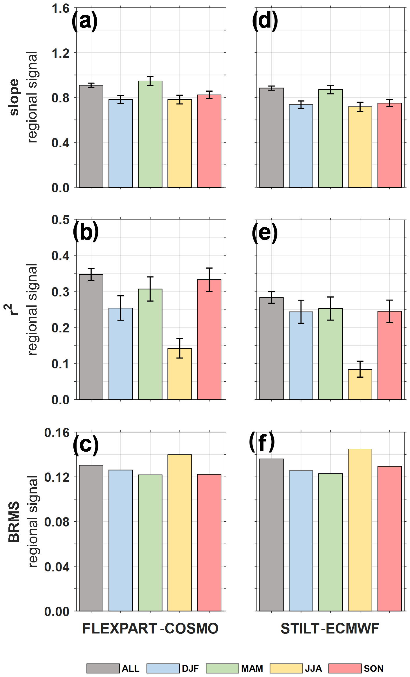
Figure 9 Summary of the regression analysis of δ¹³C–CO₂ estimation vs. observation (data are based on 3-hourly time resolution; error bars show the 95 % confidence interval). Performance parameters (slope, r² and bias-corrected RMSE – i.e. BRMS) are presented for the 4-year subset of the observation period (2012–2015) for FLEXPART–COSMO (a–c) and STILT-ECMWF (d–f) across all years (ALL) and per season (DJF, MAM, JJA, SON).

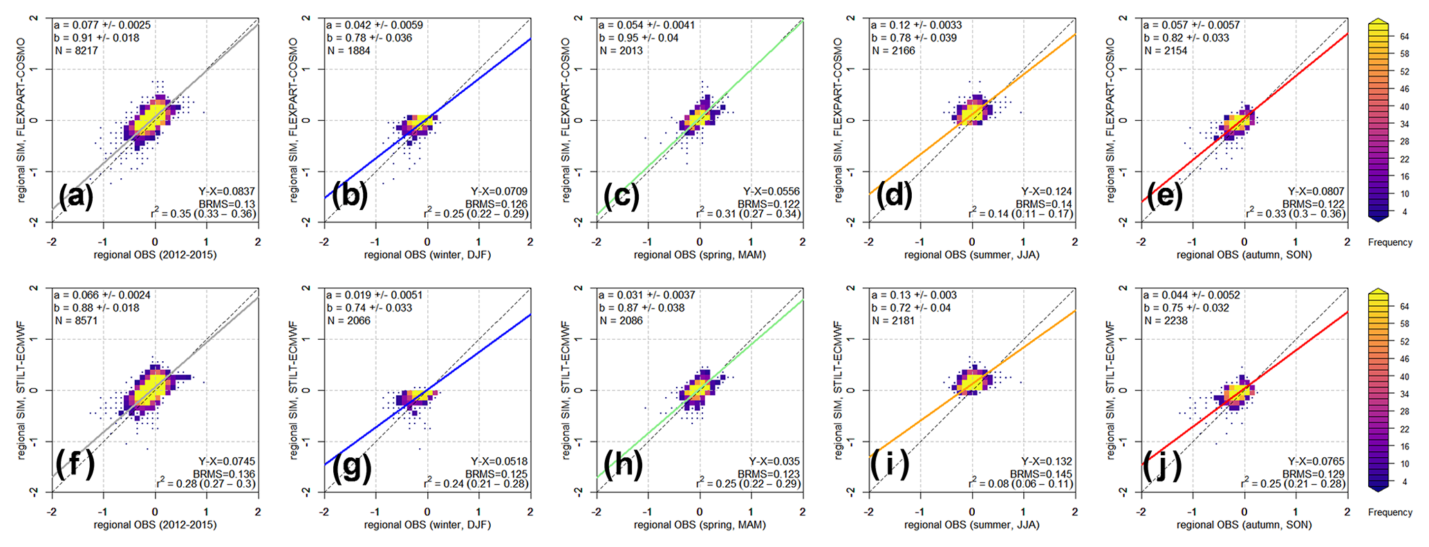
Figure 10 Heat maps of model-based regional δ¹³C–CO₂ (SIM) vs. observation (OBS) (3-hourly data) for FLEXPART–COSMO (a–e) and STILT-ECMWF (f–j) during 2012–2015, for the full year (grey), and per season (DJF – blue, MAM – green, JJA – orange, SON – red). Uncertainties in the x and y axes are taken into account in the weighted least squares regression applied here (a full-page version of this figure is available in the Supplement).

3.2.3 Observation-based source signature estimates

Observation-based δ¹³C_m values are accessible independently from simulations through a Keeling- or Miller–Tans-plot approach. However, this approach can be applied only after strict pre-selection of conditions under which the underlying hypotheses are fulfilled. Detailed descriptions of pre-requisites and limitations of this method are available in detail elsewhere (Keeling, 1958, 1961; Miller and Tans, 2003; Pataki et al., 2003; Zobitz et al., 2006; Ballantyne et al., 2011; Vardag et al., 2016). In brief, previous δ¹³C_s studies have been successful in deriving observation-based δ¹³C_m primarily under the following conditions: first, when measurements were taken close to a well-defined source location and using instrumentation with high precision (e.g., Pugliese et al., 2017) and second, when a pronounced regional signal (referred to as ΔCO₂ and computed as the difference between the CO₂ concentration at the site and background) with stable source composition was observed during stable background conditions and the regional ecosystem contribution to the observed ΔCO₂ was comparatively low (e.g., Vardag et al., 2016). Such constraints substantially limit the number of regional events that can be effectively characterized at a given location. Intensities below ΔCO₂ = 5 ppm, even at high precisions of 0.03 ‰ for δ¹³C–CO₂ and low CO₂ errors of 0.1 ppm, lead to significant fitting errors as assessed by Zobitz et al. (2006). Intensity-based filtering criteria have therefore been applied in previous studies (e.g. ΔCO₂≥ 5 ppm by Vardag et al., 2016, ΔCO₂≥ 20 ppm by Smale et al., 2020, ΔCO₂≥ 30 ppm by Pugliese-Domenikos et al., 2019, or ΔCO₂≥ 75 ppm by Pataki et al., 2003), while at JFJ ΔCO₂ reaches 30 ppm only during the most intense events. Most studies also focus on periods when photosynthetic uptake does not disturb the analysis, consequently biasing the data set to nighttime. Since a classical day–night splitting to filter ecosystem uptake is not applicable at JFJ as the received air masses are composed of integrated fluxes over day and night, such observation-based approaches are expected to be valid mainly during the cold period. However, the PBL influence at JFJ is at a minimum during the cold season. For instance, regional CO₂ intensities at JFJ are at maximum 30 ppm above the background for the 10 min averaged QCLAS data and on average occur with an intensity of ≥ 5 ppm on 35 d per year during the cold period (range: 20–50 times). This includes events reaching ≥ 10 ppm on 10 d per year (range: 2–20) and events reaching ≥ 15 ppm on only 1–6 d per year. Intensities and frequencies, however, are even lower when hourly averaged data are considered. These conditions make Keeling and Miller–Tans methods to derive observation-based δ¹³C_m particularly challenging at JFJ.

The high precision of the δ¹³C–CO₂ measurements and the high time resolution available from the QCLAS instrument allow compensating for the low ΔCO₂ and limiting fitting uncertainties to some extent. This enables us to create a moving Keeling plot in analogy to Vardag et al. (2016). We used a 5 h window to conduct the fit on hourly averaged δ¹³C–CO₂ observations. Only fits with five data points were considered (i.e. no data gaps were allowed). In addition, we tested splitting the data set into warm (April–September) and cold season (October–March), as well as demanding a minimum change in ΔCO₂ of 3 ppm within the 5 h window (with and without requiring a monotonous increase, or m.i., in concentration with time, threshold: 0.1 ppm). Finally, we filtered the resulting observation-based intercept value (δ¹³C_m) by the fitting error (4 ‰, 3 ‰, 2 ‰, and 1 ‰).

Figure 11a shows observation-based estimates from two settings: (i) results obtained without considering any predefined change in ΔCO₂ and without filtering by the intercept error (referred to as “all”) and (ii) results obtained under more stringent criteria (minimum ΔCO₂ change within a 5 h window of 3 ppm, maximum intercept error of 2 ‰ or 1 ‰). Keeling fit intercepts (δ¹³C_m) obtained without predefined criteria and without error-based filtering clearly do not provide meaningful data, as δ¹³C_m is physically meaningful only between 0 ‰, corresponding to pure cement production plumes, and − 44 ‰ corresponding to pure gaseous fuel-burning plumes (in a peculiar event, gaseous fuel-burning CO₂ may reach − 85 ‰). Most values are expected to be between − 12 ‰ and − 35 ‰ based on the simulated CO₂ composition. Indeed, using predefined fit criteria and error-based filtering yields physically meaningful δ¹³C_m from the observations at JFJ, in line with previous findings by Vardag et al. (2016) and Pugliese-Domenikos et al. (2019). Overall, the observation-based δ¹³C_m value derived with a more stringent fitting approach are in good agreement with the trends found in the independently calculated model-based data, which are also shown in Fig. 11a and Table 6. Because different combinations of predefined criteria (minimum ΔCO₂ or season-based restrictions) and filtering (based on the intercept error) may be used when deriving observation-based δ¹³C_m, we display three scenarios in Fig. 11b–d. Figure 11b highlights the effect of only filtering by intercept errors of 4 ‰, 3 ‰, 2 ‰, and 1 ‰. Instead, Fig. 11c shows the combined effect of requiring a change in ΔCO₂ > 3 ppm and filtering by intercept errors, and Fig. 11d presents data only for the cold period (October–March), limiting the disturbance of photosynthetic uptake, in addition to requiring a monotonous increase in ΔCO₂ within the 5 h window (i.e. the most stringent criteria). We may generally conclude that either more stringent intercept error thresholds (such as 1 ‰ for the settings in Fig. 11b) or, alternatively, limiting photosynthetic uptake (through demanding monotonous increase, and/or filtering for cold season or nighttime) in combination with less stringent intercept errors (e.g. 2 ‰–3 ‰ in Fig. 11d) appear to yield equally good results at JFJ, as all δ¹³C_m values are ≤ 0 ‰ and ≥ − 85 ‰ (and thus physically meaningful). The latter approach, however, discards more data. The same conclusion holds true when using 10 min averages instead of hourly data. Note that we do not expect that model-based δ¹³C_m and observation-based δ¹³C_m can be compared directly with each other, as model-based δ¹³C_m is calculated for 3-hourly resolution and, most importantly, not restricted to situations when the underlying CO₂ simulations match the CO₂ observations.

Table 6 Summary statistics of δ¹³C_m (‰, 2012–2015).

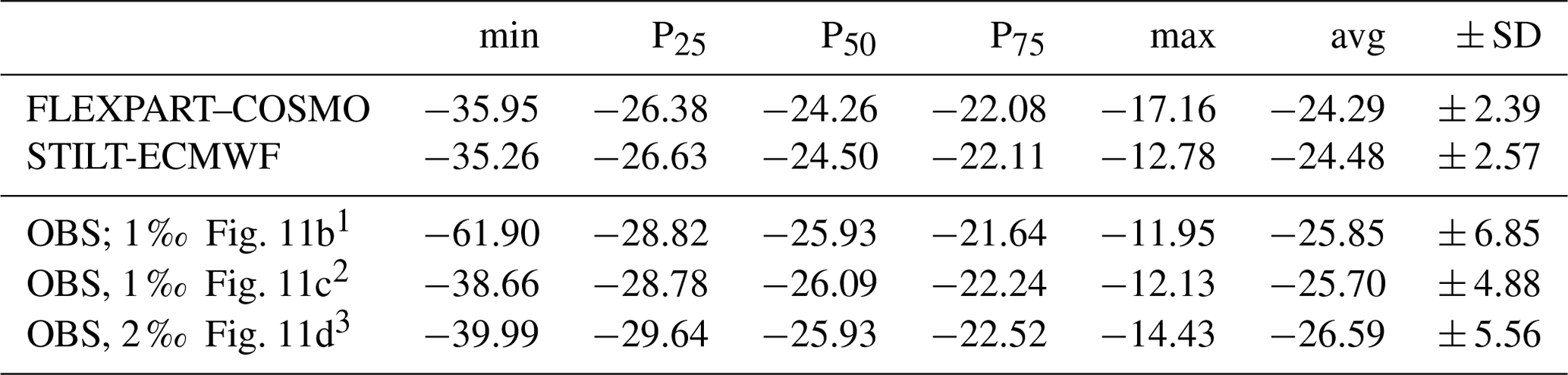
¹ Figure 11b (err < 1 ‰, w/o ΔCO₂ prerequisite, w/o seasonal filtering). ² Figure 11c (err < 1 ‰, ΔCO₂ > 3 ppm, w/o seasonal filtering). ³ Figure 11d (err < 2 ‰, ΔCO₂ > 3 ppm (m.i.), October–March).

Figure 11 Observation-based mixed source signatures, δ¹³C_m, derived from a moving Keeling approach (OBS) in comparison to model-based estimates (SIM, FLEXPART–COSMO, and STILT-ECMWF). (a) Time series of δ¹³C_m (tick marks indicate January of each year). “All” indicates that a minimum change in ΔCO₂ was not required, nor was any filtering applied. Results when requiring a minimum change of 3 ppm in ΔCO₂ within the 5 h window and a fit intercept error (err) < 2 ‰ and < 1 ‰ are provided as green and black markers (open circles represent October–March, crosses represent April–September). (b–d) δ¹³C_m hourly moving Keeling as a function of ΔCO₂ for various criteria: (b) filtering by intercept err < 4 ‰, 3 ‰, 2 ‰, and 1 ‰, (c) demanding a minimum change in CO₂ of 3 ppm and filtering by intercept err < 4 ‰, 3 ‰, 2 ‰, and 1 ‰, (d) demanding a monotonous increase in ΔCO₂ of 3 ppm within the 5 h window and filtering by intercept err < 4 ‰, 3 ‰, 2 ‰, and 1 ‰.

4 Conclusions

Greenhouse gas emission source and sink identification and quantification at remote, high-altitude sites is particularly challenging for broadly distributed, multi-source, and multi-sink compounds such as CO₂. In addition, atmospheric transport simulations are highly challenged by complex topography. Despite these difficulties, the CO₂ simulations performed on a 3-hourly basis for JFJ agree well with the observations during the multi-year period 2009–2017. Using Lagrangian particle dispersion models (LPDMs), we were able to capture 40 % of the observed regional CO₂ variability. The results from the model configurations using two different LPDMs driven by output from two different numerical weather prediction systems, FLEXPART–COSMO and STILT-ECMWF, appear to differ primarily as a function of meteorological inputs and their spatial resolution (COSMO vs. ECMWF), aside from additional variations related to the domain size and backward integration time. The LPDM implementation (FLEXPART or STILT) itself contributes comparatively small differences.

The regional CO₂ simulations suggest that JFJ's high-altitude location predominantly experiences influences from the rather nearby (within 100 km) ecosystem. This is owing to the enhanced PBL influence in summer, which overlaps with high ecosystem activity. Instead, the peak in anthropogenic fluxes during winter overlaps with substantially suppressed PBL influence and a larger (regional) footprint. Therefore, through most of the year, the ecosystem CO₂ contributions, which are composed mainly of cropland and mixed forest respiration and uptake, outweigh the anthropogenic ones composed of 90 % fossil emissions and dominated by heavy and light oil as well as natural gas. While the simulated composition resembles our hypothesis for JFJ, the extent to which ecosystem contributions outweigh anthropogenic ones is surprisingly large. Indeed, quantitatively, the models perform the CO₂ simulations best during winter and transition periods (spring–autumn). For the summer, the CO₂ simulations poorly reproduce the quantities despite the good qualitative agreement. The atmospheric transport models employed apparently suffer from their relatively coarse spatial resolution, which deteriorates model performance in summer and/or fair-weather situations, when topography-induced convection is not captured very quantitatively during daytime. Increased model resolution and improved representation of the Alpine boundary layer in both the LPDMs and the driving numerical weather prediction models will be necessary to overcome this shortcoming and to allow for more quantitative conclusions when interpreting observations during the above-mentioned conditions. However, the net ecosystem exchange fluxes themselves are also a likely source of error through inaccurate spatial distribution and VPRM parameterization of respiration and/or uptake fluxes for the (Alpine) vegetation following limited spatial resolutions of vegetation maps and possibly temperature profiles.

The simulations of regional CO₂ concentrations allow retrieving model-based mixed source signatures (δ¹³C_m) and atmospheric δ¹³C–CO₂ at JFJ. The latter agree well with the high-frequency observations. The overall δ¹³C–CO₂ correlation (28 %–35 % of variance explained) remains only slightly lower than for CO₂ (41 %–44 %). In analogy to the findings for CO₂, δ¹³C–CO₂ also shows the lowest agreement between observations and simulations during the summer. We relate this primarily to the poorly reproduced CO₂ quantities in summer, although the assumption of source signatures (δ¹³C_s) and the estimate of the background (δ¹³C_b) provide additional uncertainties. For instance, our δ¹³C_s estimates do not consider geographic variations in fuel-specific δ¹³C_s and ecosystem values are not specific to photosynthetic pathways. Dedicated maps that allow separating C₃ and C₄ vegetation in the VPRM would allow for even better representing the forward δ¹³C_m of CO₂. In addition, the simulations would benefit from further optimizations in deriving the background δ¹³C_b.

Observation-based assessments of δ¹³C_m are challenging at JFJ owing to the low signal-to-background ratios and the integration of fluxes over day and night, which substantially limited the data set. Yet, physically meaningful values were obtained. A further disaggregation of observation-based δ¹³C_m using mass balance approaches and assumptions for the endmembers in order to learn more about the CO₂ regional composition for any further comparison to the simulated CO₂ regional composition was not attempted here, given the small number of observation-based δ¹³C_m values obtained. This may be the focus in future studies. However, we expect that it will remain challenging to disentangle fuel and ecosystem respiration signals from observation-based δ¹³C_m alone, considering that the simulated regional CO₂ fractions at JFJ indicate approximately equal amounts even during the winter and that solid and liquid fuel emission δ¹³C_s endmember assumptions overlap with C₃ plant respiration signatures. Thus, while δ¹³C_s source apportionment approaches prove meaningful among either the anthropogenic or the ecosystem carbon pool, they are of more limited use as a singular tracer when the carbon pools are mixed.

The simulated regional CO₂ composition at JFJ suggests that further analyses would benefit from a multi-tracer approach, in combination with the continuous CO₂ and δ¹³C observations presented herein. Additional parameters may include CO, atmospheric potential oxygen (APO), and ¹⁴C as a combustion or fossil fuel tracer, as well as carbonyl sulfide (COS) and δ¹⁸O–CO₂ as ecosystem tracers. Indeed, CO, APO, COS, and δ¹⁸O–CO₂ observations are available at high time resolution at JFJ and may be investigated in future, although determining their regional and background contributions will still be challenged by the low signal-to-background ratios. The biweekly integrated ¹⁴CO₂ data currently available for JFJ do not allow distinguishing regional from background contributions. Highly time-resolved ¹⁴CO₂ measurements or grab sampling during periods with intense regional CO₂ influences would be highly valuable and are foreseen to be implemented at JFJ as part of the European-wide flask sampling strategy of the ICOS Research Infrastructure. Moreover, specific episodes at JFJ that represent air masses of particular regional CO₂ composition may (also) be identified based on continuous δ¹³C observations in a multi-tracer manner in future studies.

Appendix A: Transport dynamics analysis for JFJ

We performed a dedicated set of simulations to characterize the atmospheric transport in backward LPDM simulations for JFJ as represented by different models in different configurations for 2009–2017. In order to analyse source sensitivity dependencies on domain size (western Europe – “small” vs. Europe – “large”), LPDM implementation (FLEXPART vs. STILT), and meteorological input fields and associated spatial resolution (COSMO vs. ECMWF), we used four different combinations of these three parameters (Table A1). The simulations are based on one assumed input field of idealized, positive CO₂ fluxes, which were kept constant in time and space for seven VTs based on the maps underlying the VPRM. This analysis is designed to study atmospheric transport of chemically passive tracers released rather uniformly over the European continent to the high Alpine site, and the obtained signals serve as a measure of PBL influence of JFJ. It includes the total of the synthetic CO₂ concentration time series from all seven VTs, alongside sub-groups comprising (a) cropland, (b) mixed forest, and (c) the total of the remaining five VTs. Studying the VT sub-groups gives insight into the influence of spatial distributions of the sources within the domains under the given assumptions of uniform fluxes. This transport dynamics analysis supports the interpretation of the results presented in Fig. 1.

Figure A1 provides the multi-annual monthly means of the 3-hourly tracer concentrations at JFJ and highlights the sensitivity to domain size (E1 vs. E2), meteorological input fields and spatial resolution (E2 vs. E3), LPDM implementation (E1 vs. E4), and combinations of these (E3 vs. E4). Overall, we find that the synthetic CO₂ concentrations simulated at JFJ vary between the different models and configurations, as well as with seasonality and diurnal cycle. The analyses indicate a significant seasonality in the PBL influence for all four configurations. Higher tracer concentrations are observed during the warm period (April–September) and relatively lower tracer concentrations during the colder period (October–March). This confirms the generally stronger vertical transport during warm (and possibly sunny) days. Further, meteorological input fields and related spatial resolution (ECMWF vs. COSMO, i.e. E2 vs. E3) appear to have a larger influence compared to the LPDM implementation itself (FLEXPART vs. STILT, i.e. E1 vs. E4), and intensity discrepancies between the models used in the main text (E3, E4) are largest in winter, followed by summer, and smallest during transition periods. Concerning the domain size, we find differences between different VT classes, which is owing to their heterogeneous spatial distribution as some VT classes are present predominantly inside (e.g. mixed forest) or outside (e.g. deciduous forests) the smaller domain boundaries; compare Figure S2. The smallest discrepancy was thus found for mixed forest (essentially 0 %), and a larger discrepancy (on average −15 %) was found for cropland at the artificially assumed spatially and temporally constant fluxes. The influence of the LPDM implementation itself (FLEXPART vs. STILT, i.e. E1 vs. E4) appears to be smaller than that of the meteorological fields and spatial resolution, generating differences mainly during winter periods, when FLEXPART-ECMWF yields a higher relative signal compared to STILT-ECMWF. In Fig. A2, we present the PBL influence on diurnal timescales, with up to 1.4 times higher synthetic CO₂ concentrations at JFJ during the afternoon and evening (maximum around 16:00–20:00, UTC + 1) compared to the morning (minimum around 10:00, UTC + 1). This is observed for FLEXPART–COSMO (E3) as well as STILT-ECMWF (E4), and it is particularly pronounced during summer (June–August).

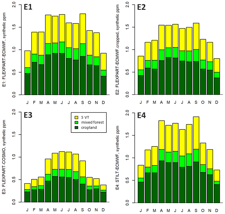
Figure A1 Mean monthly PBL sensitivity (JFJ, 2009–2017) towards (i) domain size (E1 vs. E2), (ii) meteorological input fields and spatial resolution (E2 vs. E3), (iii) LPDM implementation (E1 vs. E4), and (iv) combinations (E3 vs. E4).

Table A1 Model combinations for transport dynamics analysis. E3 and E4 are the model configurations as used for the CO₂ concentration simulation in the main text.

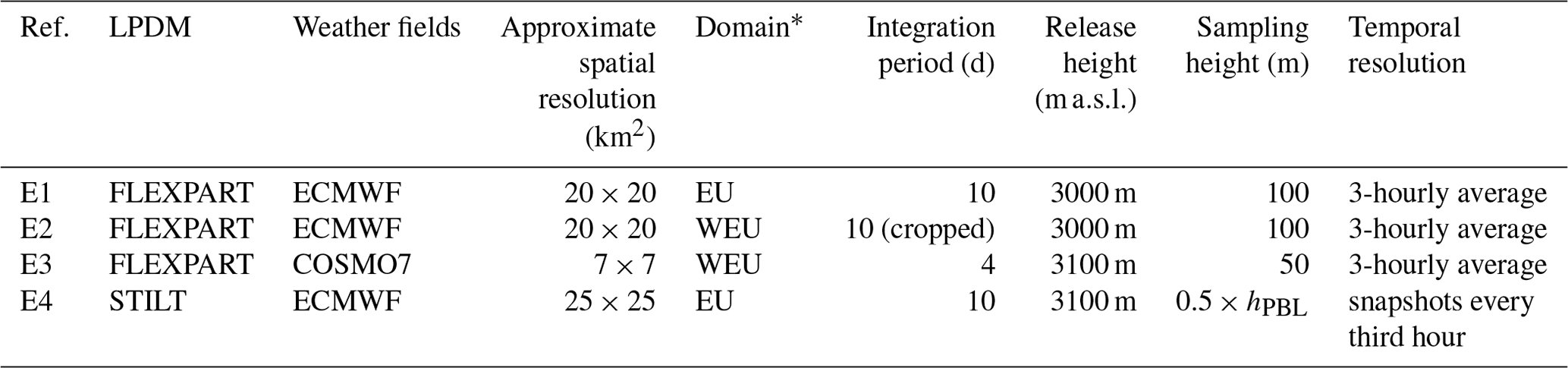
^* EU and WEU refer to 33^∘ N–73^∘ N, −15–35^∘ E and 36.06–57.42^∘ N, −11.92–21.04^∘ E, respectively.

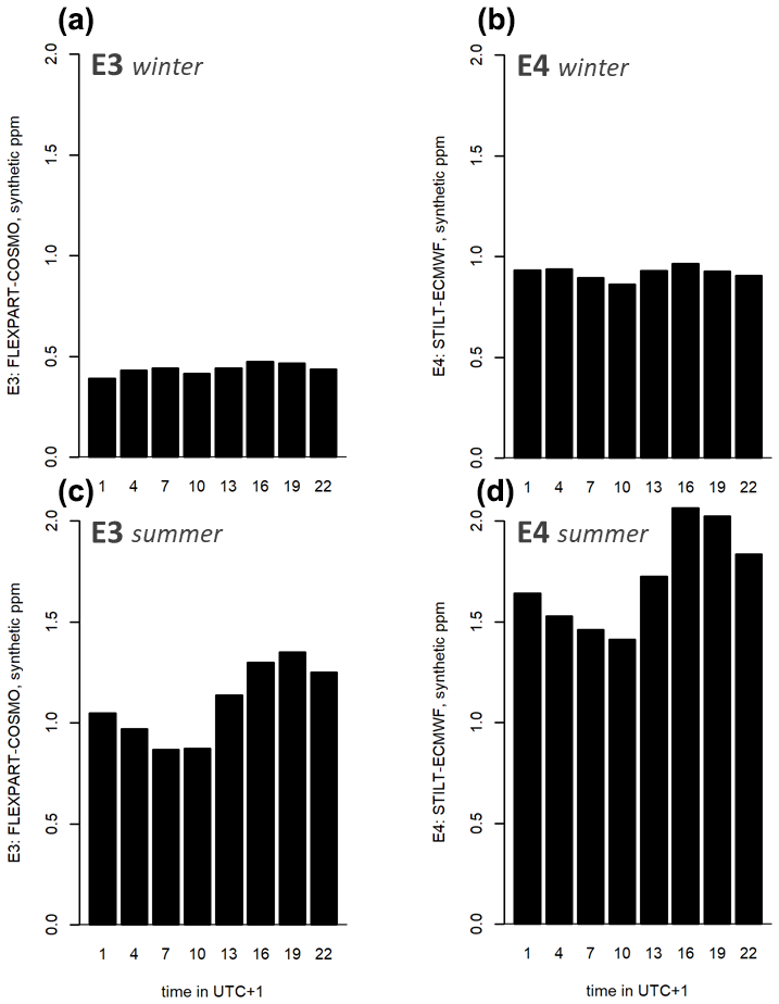
Figure A2 Mean diurnal PBL sensitivity (JFJ; winter, DJF, a, b and summer, JJA, c, d) for the period 2009–2017 for (a) FLEXPART–COSMO (E3) and (b) STILT-ECMWF (E4).

Appendix B: Abbreviations and definitions

fb	CO2 concentration in the background, expressed in ppm
fs	Regional contribution to the CO2 concentration per category, expressed in ppm
CO2.regional	Sum of all regional contributions to the CO2 concentrations (fs)
CO2.total	Sum of CO2.regional and JCS-based CO2 background (fb)
CO2.anthr	CO2 concentration associated with all anthropogenic (anthr) categories
CO2.cement	CO2 concentration associated with cement production
CO2.fuel	CO2 concentration associated with all fuel categories
CO2.gee	CO2 concentration associated with gross ecosystem exchange (i.e. ecosystem uptake) (gee)
CO2.nee	CO2 concentration associated with net ecosystem exchange (nee)
CO2.resp	CO2 concentration associated with gross ecosystem respiration (resp)
δ13Ca	δ13C–CO2 estimate for atmospheric CO2 at JFJ ‰
δ13Cb	δ13C–CO2 estimate for the background CO2, ‰
δ13Cm	δ13C–CO2 mixed source signature for all δ13Cs weighted with the CO2 concentration (fs), ‰
δ13Cs	δ13C–CO2 source signature, ‰
COSMO	Consortium for Small Scale Modelling
ECMWF	European Centre for Medium-Range Weather Forecasts
EDGAR	Emissions Database for Global Atmospheric Research
FLEXPART	Flexible Particle Model
JCS	Jena-CarboScope-based background estimate
LPDM	Lagrangian particle dispersion model
MACC-TNO	Monitoring Atmospheric Composition and Climate (provided by TNO)
QCLAS	Quantum cascade laser absorption spectrometer
STILT	Stochastic Time-Inverted Lagrangian Transport
VPRM	Vegetation and Photosynthesis Respiration Model