the Creative Commons Attribution 4.0 License.
the Creative Commons Attribution 4.0 License.
 | 21 Jan 2022
A case study on the impact of severe convective storms on the water vapor mixing ratio in the lower mid-latitude stratosphere observed in 2019 over Europe
Dina Khordakova
Jens-Uwe Grooß
Rolf Müller
Paul Konopka
Andreas Wieser
Martina Krämer
Martin Riese
Extreme convective events in the troposphere not only have immediate impacts on the surface, but they can also influence the dynamics and composition of the lower stratosphere (LS). One major impact is the moistening of the LS by overshooting convection. This effect plays a crucial role in climate feedback, as small changes of water vapor in the upper troposphere and lower stratosphere (UTLS) have a large impact on the radiative budget of the atmosphere. In this case study, we investigate water vapor injections into the LS by two consecutive convective events in the European mid-latitudes within the framework of the MOSES (Modular Observation Solutions for Earth Systems) measurement campaign during the early summer of 2019. Using balloon-borne instruments, measurements of convective water vapor injection into the stratosphere were performed. Such measurements with a high vertical resolution are rare. The magnitude of the stratospheric water vapor reached up to 12.1 ppmv (parts per million by volume), with an estimated background value of 5 ppmv. Hence, the water vapor enhancement reported here is of the same order of magnitude as earlier reports of water vapor injection by convective overshooting over North America. However, the overshooting took place in the extratropical stratosphere over Europe and has a stronger impact on long-term water vapor mixing ratios in the stratosphere compared to the monsoon-influenced region in North America. At the altitude of the measured injection, a sharp drop in a local ozone enhancement peak makes the observed composition of air very unique with high ozone up to 650 ppbv (parts per billion by volume) and high water vapor up to 12.1 ppmv. ERA-Interim does not show any signal of the convective overshoot, the water vapor values measured by the Microwave Limb Sounder (MLS) in the LS are lower than the in situ observations, and the ERA5 overestimated water vapor mixing ratios. Backward trajectories of the measured injected air masses reveal that the moistening of the LS took place several hours before the balloon launch. This is in good agreement with the reanalyses, which shows a strong change in the structure of isotherms and a sudden and short-lived increase in potential vorticity at the altitude and location of the trajectory. Similarly, satellite data show low cloud-top brightness temperatures during the overshooting event, which indicates an elevated cloud top height.
- Article
(8726 KB) - Full-text XML
- BibTeX
- EndNote


Extreme weather events tend to not only have immediate consequences on nature and the built environment but also greater long-term impacts on climate and ecosystems. Such extreme events include long-lasting drought phases, extreme precipitation, heat and cold waves (periods of extremely warm or extremely cold air or sea surface temperature), as well as unusually strong hurricanes and storms. Events that have previously been considered extreme and rare are becoming increasingly frequent and have the tendency to become the new routine (Walsh et al., 2020). Extreme convective events in the troposphere also have an influence on the lower stratosphere (LS). One of the impacts on the LS is the in-mixing of tropospheric air masses by overshooting convection and the coherent transport of moisture into the dry lower stratosphere. Stratospheric water vapor is determined by the entry mixing ratio of H2O at the tropopause and a chemical contribution by the oxidation of CH4 to H2O (Randel et al., 1998; Rohs et al., 2006). Through the analysis of multiple data sets, the water vapor background value in the LS is found to be ≈ 5 ppmv (parts per million by volume; Pan et al., 2000; Hegglin et al., 2009); any stronger enhancements of water vapor in the LS are likely caused by the in-mixing of tropospheric air masses (Smith et al., 2017; Wang, 2003). Stratospheric water vapor influences the climate and the chemistry of the atmosphere and plays a significant role in the positive feedback of global climate warming (Smith et al., 2017; Dessler et al., 2013). The feedback effect of water vapor in the stratosphere is about 0.24 W m−2 for each 1 ppmv increase, assuming an equal distribution globally (Solomon et al., 2010; Forster and Shine, 1999). Even small changes in the water vapor mixing ratio in the upper troposphere and lower stratosphere (UTLS) result in large radiative effects (Solomon et al., 2010; Riese et al., 2012). However, the magnitude of the impact of stratospheric water vapor, when a coupled global model is used, is still under discussion. Huang et al. (2020) and Wang and Huang (2020) show that the radiative effect of stratospheric water vapor is balanced by a decrease in high clouds and an increase in the upper tropospheric temperature. A moistening of the lowermost stratosphere also has an impact on the chemistry of this region. Stratospheric water vapor is a source of HOx radicals which catalytically destroy ozone and enhance the reactivity of stratospheric sulfate aerosol particles. Anderson et al. (2012) have hypothesized that the moistening of the lowermost stratosphere by convective overshooting can lead to severe ozone depletion in summer in the mid-latitudes through heterogeneous chlorine activation. However, in a detailed analysis of the relevant chemical processes, Robrecht et al. (2019, 2021) conclude that convective moistening only has a minor impact on stratospheric ozone and the mid-latitude ozone column. The contribution of overshooting convection to the moisture budget of the lower stratosphere and a potential increase of overshooting convection with global warming is still under discussion (Jensen et al., 2020).
It was shown in a previous work that deep convective events can penetrate the tropopause and have a significant impact on the water vapor concentration in the lower stratosphere (Smith et al., 2017). Jensen et al. (2020) showed that the primary region for direct convective hydration of the extratropics is located over North America. These direct injections over the North American continent (NA) have been evaluated in several case studies (Weinstock et al., 2007; Homeyer and Kumjian, 2015; Homeyer et al., 2017; Smith et al., 2017), and the long-term behavior was analyzed. Phoenix and Homeyer (2021) simulated two kinds of convection, namely one representing springtime convective events and one representing convective events typical for summertime. The study shows that simulations representing the springtime convective event lead to an increase of about 20 % in the average water vapor mixing ratio in the UTLS, while the summertime simulation lead to lower increase. Fischer et al. (2003) show data displaying the troposphere to stratosphere transport of tropospheric tracers caused by convective storms over Italy, and Hegglin et al. (2004) analyze a case study of the injection of tropospheric air into the LS by a large convective system over the Mediterranean area.
In our case study, we investigate the transport of water vapor into the extratropical lower stratosphere injected by deep convective events over Europe, using observations within the MOSES (Modular Observations Solutions of Earth Systems) measurement campaign. MOSES aims to investigate extreme weather events across the Earth compartments in order to understand the short- and long-term influences of such events (Weber and Schuetze, 2019). In situ measurements were made during early summer in 2019 at a mid-latitude site in the eastern part of Germany. Balloon-borne light-weight instruments recorded water vapor, ozone, temperature, and pressure immediately before and after a thunderstorm with strong convection that passed the measurement site. Such observations can be rarely made due to the short-term forecast of convective events. In total, two cases of overshooting convection on 2 consecutive days (10 and 11 June 2019) are discussed in this study. Both cases show that significant amounts of water vapor can be transported into the lower stratosphere by deep convective events over Central Europe and not just in the North American and Asian monsoon regions. We show that water vapor mixing ratios of the same order of magnitude as the data recorded over NA can also be found deep in the extratropics over Central Europe. Using back trajectories together with ERA5 reanalysis and Microwave Limb Sounder (MLS) data, we analyze the entry point of the tropospheric air masses transported into the stratosphere.
Section 2 introduces the instruments and methods used, while Sect. 3.1, 3.2, and 3.3 describe the two events and the results of the balloon profile measurements. In Sect. 3.4, the data are compared to ERA5 reanalysis, while in Sect. 3.5, using backward trajectories and satellite data, the time and location of the origin is discussed. In Sect. 4, the results are discussed, while Sect. 5 concludes the outcome of the study.
2.1 Balloon measurements within MOSES
In this study, we analyze data collected during a MOSES measurement campaign in 2019. The campaign took place from the middle of May to the end of July as part of a collaboration of eight Helmholtz Association research centers. The objective of the measurement campaign was to capture extreme hydrological events throughout the following different Earth compartments: atmosphere, ground, and running waters. In the Eastern Ore Mountains in Germany, close to the city of Dresden, a 3-month measurement campaign, with intense operational phases (IOPs), was performed. During these IOPs, the teams operated on demand to capture the development and cycle of convective events. Our main measurement site was located adjacent to the village of Börnchen in the low mountain range at 50.80∘ N and 13.80∘ E. The team from Forschungzentrum Jülich (FZJ) focused on small-scale deep convective events and their impact on the stratosphere. During the campaign period, two of these events occurred and were observed with balloon-borne measurements. Figure 1 schematically shows the measurement procedure. As a convective cell was approaching the measurement site, two weather balloons were launched to measure the state of the atmosphere. The first balloon was launched just before the convective cell reached the measurement site; the second balloon was launched immediately after the storm cell passed the measurement site and as soon as the rain stopped.

Figure 1Schematic of the measurement strategy. A balloon is launched right before and immediately after a deep convective event has passed the measurement site. On the right-hand side, the approximate ozone (blue) and temperature (yellow) climatological profiles are shown. The amount of water vapor transported into the stratosphere is investigated by the difference between the two profiles above the lapse rate tropopause, according to the WMO (World Meteorological Organization) definition.
There were two kinds of measurement balloons used. The first version is a 200 g latex balloon equipped with a Vaisala radiosonde RS41-SGP, which recorded the location of the balloon and the altitude, pressure, temperature, and moisture of the atmosphere and transmitted the data to the ground station at the measurement site. The temperature sensor of the radiosonde has an uncertainty of 0.3 K below 16 km and 0.4 K above. The uncertainty of the humidity sensor is given as 3 %, and the pressure sensor has an uncertainty of 1.0 hPa at ambient pressure above 100 hPa, 0.3 hPa between 10 and 100 hPa, and 0.04 hPa below 10 hPa. Survo et al. (2014) report a temperature dependency of the humidity sensor uncertainty which does not exceed 3 % RH at temperatures below −80 ∘C and RH below 30 %. The second version is a 1500 g balloon also equipped with a payload carrying multiple in situ instruments. An ECC (electrochemical concentration cell) instrument (Smit et al., 2007) was used to measure ozone mixing ratios with an uncertainty of ≈ 5 % below 20 km (Smit et al., 2007; Thompson et al., 2019; Tarasick et al., 2021), and a CFH (cryogenic frost point hygrometer; Vömel et al., 2007) was used to measure the low water vapor concentration prevailing in the tropopause region and in the stratosphere. The uncertainty of the CFH instrument is given as 4 % in the troposphere and below 10 % in the stratosphere. The payload also contained a Compact Optical Backscatter Aerosol Detector (COBALD) to measure backscatter from different types of particles during nighttime (Brabec et al., 2012). This is referred to as a large payload in the following. However, the measurements taken by the COBALD instrument were not used for the analysis presented here. A picture of the entire payload with the radiosonde, ECC, CFH, and COBALD is shown in Fig. A1. The payload is adapted from the setup used by the GRUAN (Global Climate Observing System (GCOS) Reference Upper-Air Network) setup (Dirksen et al., 2014). A more detailed description of the instruments can be found in Appendix A.
Figure 2 displays all available water vapor profiles (18 profiles available) measured in the mid-latitudes by the authors with the RS41 and the CFH as a reference instrument between 2018 and 2020 (see Appendix A2). When considering data up to 20 km, the correlation of the RS41 and CFH data is 0.975, and no general bias is visible. However, the data spread around the 1-to-1 line in Fig. 2 reveals some time differences of up to around 100 % in the altitude range of the UTLS (<20 km), mainly due to the slower time response under cold conditions. But, for the purposes of this analysis, the absolute accuracy of the RS41 sensor is less important than its sensitivity to detecting abrupt changes with a magnitude far greater than its measurement uncertainty. The deviation between both instruments increases above ≈ 20 km, and the correlation of the data is reduced to 0.45 for data points measured between 20 and 30 km. In the mid-stratosphere, the low humidity in combination with low pressure does not allow reliable measurements to be conducted with the RS41. Therefore, these astonishingly good results offer reliability when using accurate RS41 humidity measurements up to a height of 20 km, and these are used in this study in the case of flights that were performed without the CFH instrument.
During the first event, on 10 June 2019, we launched one radiosonde and one large payload, while only five radiosondes were used during the second event, on 11 June 2019, due to logistical reasons. In most cases, the balloons reached far into the stratosphere, reaching altitudes of up to 22 km with radiosondes only and up to 35 km with larger balloons, which were equipped with the abovementioned instruments and captured the entire UTLS region during ascent and descent. During the first balloon launch of the first convective event, the connection to the radiosonde was lost for about 20 min, and the data between 11 and 18 km altitude were lost during the ascent, but all other sounding data were complete.
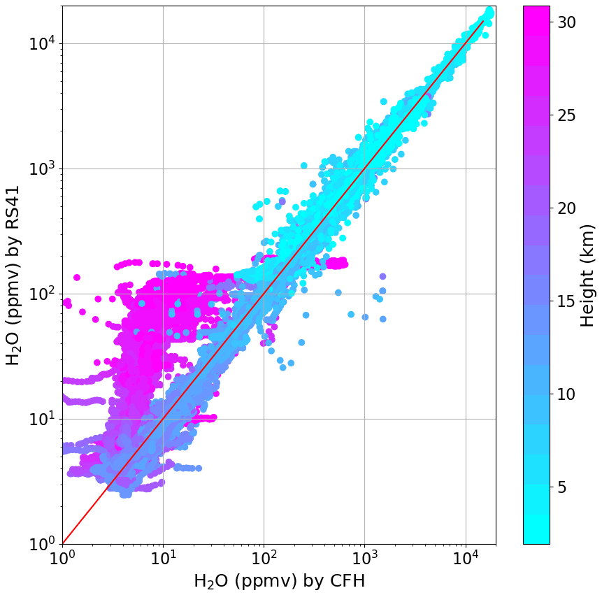
Figure 2Correlation of water vapor mixing ratios measured simultaneously by RS41 and the CFH. The color code represents the altitude of the measurement. All data measured by the authors between 2018 and 2020 are used.
2.2 Aura Microwave Limb Sounder (MLS)
The Microwave Limb Sounder is an instrument operating on board the Aura satellite. The Sun-synchronous polar orbit satellite has an inclination of 98∘ and an Equator crossing time of 13:45 UTC ±15 min. It was launched on 15 July 2004 and has been operating ever since. The measurements are in limb-viewing geometry on the A-train orbit and are in the spectral range of thermal emission; thus, day- and nighttime measurements are available. Temperature and pressure are retrieved from the 118 GHz band, water vapor from the 190 GHz band, and ozone and CO from the 240 GHz band (Schoeberl et al., 2006; Waters et al., 2006). In this work, data from the version 4 retrieval algorithm were used to obtain the data presented. In this study, we show ozone, water vapor, and CO mixing ratios. MLS version 4 data are provided on 36 different pressure levels, ranging from 316 to 0.002 hPa, as described in Livesey et al. (2017), and the data quality is described in Pumphrey et al. (2011). One of the main improvements of version 4 is the improved cloud detection, which excluding cloudy radiances causing corrupted profiles. This improvement increases the quality of our data set, as our area of interest is covered with clouds.
2.3 ECMWF ERA5
The European Centre for Medium-Range Weather Forecasts (ECMWF) produces numerical weather forecasts and provides a meteorological data archive. In this study, we use ERA5, which is a global reanalysis, covering the period from 1979 until present (Hersbach et al., 2020). The spatial resolution is about 30 km and contains 137 vertical levels from the surface to an altitude of 80 km. In this work, ERA5 reanalysis data from May to June 2019 were used with an hourly temporal resolution. The reanalysis data set was interpolated to isentropic levels and potential vorticity (PV) was added to the individual isentropic levels (Ertel, 1942). In the Northern Hemisphere, PV values above 2 PVU are typical for the stratosphere, while values below 2 PVU are typical for the troposphere, where 1 PVU = km2 kg−1 s−1 (Kunz et al., 2011). Additionally, we calculated the vertical gradient of potential temperature, which is part of the PV definition, and defined as follows:
where g is the gravitational acceleration, ζ is the relative isentropic vorticity, f is the Coriolis parameter, θ is the potential temperature, and p is the pressure. The vertical gradient of potential temperature is and is hereafter referred to as dTheta. dTheta is negative by definition, as with decreasing pressure, the potential temperature increases in a stable atmosphere. In the troposphere, potential temperature shows only a slight increase and can, thus, be considered as a constant relative to the steep increase that occurs above the tropopause.
2.4 Trajectory calculation
In order to calculate backward and forward trajectories of the measured air masses the trajectory module of the three-dimensional chemistry transport model CLaMS (Chemical Lagrangian Model of the Stratosphere; McKenna et al., 2002) was used. The trajectories were initialized at pressure levels between 135 and 175 hPa in steps of 5 hPa, which encompasses the pressure level of the maximum water vapor enhancement measured for both cases using the same method as described in Rolf et al. (2018). Each trajectory was calculated for both 100 h backward and 100 h forward in time. The trajectory calculation with CLaMS is based on the ERA5 horizontal wind fields and diabatic heating rates with an hourly output. In addition, temperature, pressure, PV, water vapor, and ozone mixing ratios, as well as convective available potential energy (CAPE), are interpolated from ERA5 onto the coordinate of the trajectories.
3.1 Meteorological situation at the time of the case study
From 10 to 12 June 2019, multiple severe convective storms developed over Germany. During these events, hail with a diameter of up to 6 cm was observed, and heavy rain with a daily amount of 100 mm was measured. Wilhelm et al. (2020) describe this series of convective storms in detail. In our study, we define the events that precede the measurements taken on the evening of 10 June 2019 as case 1 and the ones preceding the measurements taken in the evening of 11 June 2019 as case 2. The storm of case 1 passed the measurement site at approximately 20:00 UTC on 10 June 2019. On the previous day, a low pressure system with warm and humid air was brought to Central Europe, while a strong wind shear caused by a lee depression was located over the Czech Republic. A first convective storm developed in the northeastern part of Italy and progressed westwards until it started dissipating at around 08:00 UTC over the northwestern part of Italy. Later in the day, in combination with strong solar radiation, these storm precursors caused the first significant convective cell over Memmingen (southern Germany) at around 16:00 UTC. This cell developed into a supercell and caused severe damage in northern Munich at around 17:45 UTC. Multiple supercells subsequently formed, combined over eastern Germany, and later moved towards Poland and the Baltic Sea. The formation of supercells passed the measurement site in the Eastern Ore Mountains, and balloon profiles were taken before and after the storm cell passed. The first balloon was launched at approximately 18:00 UTC (hereinafter referred to as “profile before”) and equipped only with a radiosonde. The second balloon launch, with a large balloon payload, took place at 01:00 UTC on the next day, shortly after the thunderstorm passed.
On 11 June 2019, the already warm and humid air mass was heated up to 33 ∘C at ground level in the afternoon. At 12:00 UTC, a first convective cell developed over the Slovenian–Austrian border and further developed over the next 7 h to a mesoscale convective system (MCS) covering almost all of Austria and Slovenia. With an offset of approximately 1 h, another convective cell emerged over the center of northern Italy, and multiple smaller cells developed over the German–Czech border, starting at around 15:00 UTC. All of these convective cells increased spatially throughout the day and unified to an MCS covering the entirety of eastern Germany. At around 17:39 UTC, a first cell developed between Dresden and Bautzen. Hail with particles reaching a diameter of up to 4 cm was observed. This event, subsequently referred to as case 2, was captured only with radiosondes that were launched every 3 h, starting from 13:00 UTC, until midnight when the last radiosonde was launched after the storm had passed the measurement site.
3.2 Water vapor injection captured by balloon profiles
The measurement results of cases 1 and 2 can be seen in Figs. 3 and 4. The measurements before and after the respective extreme convective event (hereinafter referred to as “the event”) are displayed with ascending and descending profiles, where available. The UTLS intercept is shown with pressure levels between 240 and 90 hPa and potential temperatures ranging between 320 and 420 K. A sharp transition from the characteristics of tropospheric to stratospheric air masses is clearly discernible in all figures. The lapse rate tropopause (LRT), as defined by the World Meteorological Organization (WMO), is at a pressure level of 203 hPa before and at 196 hPa after the convective event for case 1 (see Fig. 3) and at 194 hPa before and at 200 hPa pressure level after the event for case 2 (see Fig. 4). In all cases, the cold point tropopause (CPT) is slightly (4–20 hPa) above the LRT. For case 1, the sharp transition from the troposphere to the stratosphere is discernible by a distinct change in the course of the temperature. Additionally, an abrupt increase in ozone and a decrease in the water vapor mixing ratio towards the stratospheric background level below 5 ppmv show the difference between the two regimes. Between pressure levels of 180 and 162.5 hPa, which correspond to potential temperature levels of 345 and 357.5 K, the water vapor mixing ratio fluctuates between 5 and 7.4 ppmv and between 6 ppmv and 14.5 ppmv, as measured by the radiosonde and the CFH, respectively, before it attains the stratospheric background value of ≈ 4–5 ppmv, which is reached within all case 1 profiles below the 160 hPa or 360 K level. A background value of ≈ 5 ppmv agrees well with results of previous studies (Pan et al., 2000). The ascent profile measured after the event shows a strong increase in water vapor measured by the radiosonde and by the CFH above the level of 155 hPa or 365 K. The maximum value measured by the RS41 is 7.0 (± 10 %) ppmv, and the maximum value measured by the CFH is 8.6 (± 6 %) ppmv. The lagging response time of the RS41 may explain most of the difference between the CFH and the radiosonde observations as described in Appendix A3. Above the water vapor enhancement, at 143 hPa or 375 K, the mixing ratio decreases rapidly again to the background value below 5 ppmv. This peak is only apparent in the ascending profile of the measurement. The descending profile shows no peak signatures in either the CFH or in the RS41 water vapor measurements. As the horizontal distance between the location during ascent and descent at this altitude is only 60 km and about 2 h (00:59/02:49 UTC) time difference, the enhancement in the water vapor mixing ratio is a localized feature. In Fig. 3a and b, the vertical extent of the discussed water vapor peak is framed with a gray background.
A striking peak in the ozone profile is evident at a similar level to the peak in water vapor. With a lower edge at 162 hPa or 359 K and an upper edge at 145 hPa or 373 K, the ozone peak starts at a lower level compared to the water vapor enhancement but is limited by the same upper edge. This ozone peak is not associated with the overshooting event, and the cause is discussed in Sect. 3.3. Within this peak, a steep decrease in the ozone mixing ratio occurs very sharply at the same potential temperature level as the sudden appearance of the water vapor peak, which becomes especially evident in Fig. 4b. This is a major indicator of the in-mixing of tropospheric air into this level, which has a low concentration of ozone and a high amount of water vapor. Figure 3b clearly demonstrates that the air mass with increased water vapor also has diluted mixing ratios of ozone as the ozone mixing ratio decreases sharply at the same level at which the strong increase in water vapor appears. Further evidence of the tropospheric origin of the air mass can be seen when considering the temperature profile. The temperatures typically increase with altitude throughout the stratosphere. In the measured ascent profile, after the temperature dropped to 207.9 K at the CPT, it increases until it reaches 220.4 K at a potential temperature level of 365 K, where it declines sharply to 218.63 K. In Fig. 3b, it becomes evident that the larger temperature dip of ≈ 2 K occurs suddenly at 365 K, which is the same level as the strong decrease within the ozone peak. The temperature drop within the water vapor enhancement might be a result of mixing with the strongly adiabatic cooled tropospheric air within the overshooting top and the warmer stratospheric air masses in the surrounding. In addition, the evaporation or sublimation of cloud particles in this warmer and drier mixing area around the overshooting top can also lead to further cooling.
Case 2 presents a slightly different background atmosphere than case 1. The transition from the tropospheric to the stratospheric regime proceeds less abruptly, as depicted in Fig. 4a and b (the water vapor mixing ratios of the flight launched at 13:14 UTC, with the RS41 corrected for an offset bias). The CPT is further above the LRT, and the CPT temperature minimum is less distinct. For case 2, multiple background profiles exist, launched throughout the day, before the occurrence of the convective event in the night. To simplify the figure, only the tropopause of the last profile before the event is shown in Fig. 4a and b. The water vapor profile shows a similar feature as case 1. As the water vapor mixing ratio converges to the background value, it is first disrupted by a peak reaching a value of 6.5 ppmv and returning to the background value at a pressure or potential temperature level of 153 hPa or 365 K, respectively. At this elevation, a second peak is discernible with water vapor mixing ratios of 12.1 ppmv (± 10 %) at 143 hPa or 371 K. As multiple balloon launches were performed throughout the day, an increase in background water vapor mixing ratios with progressing launch time is evident. Balloon profiles launched at 19:00 and 22:00 UTC show a slight water vapor enhancement up to 5.5 ppmv (± 10 %), which is at the same level as the main peak measured in the ascending profile after the event. The descending profile also shows an increase in the water vapor mixing ratio at the same pressure altitude as the ascending profile. However, this peak is wider and only about half the amplitude. Similar to case 1, the temperature measured during ascent shows a sharp decrease of 2 K at the potential temperature level of the highest water vapor mixing ratio value of the peak. In case 2, the water vapor peak is more spiked compared to the rectangular profile visible in case 1 (shown in Fig. 3a and b). It is of further interest that all temperature profiles measured on 11 June 2019 clearly show a second tropopause at about 110 hPa, while the temperature profiles of case 1, measured only a couple of hours before, do not show such a structure.
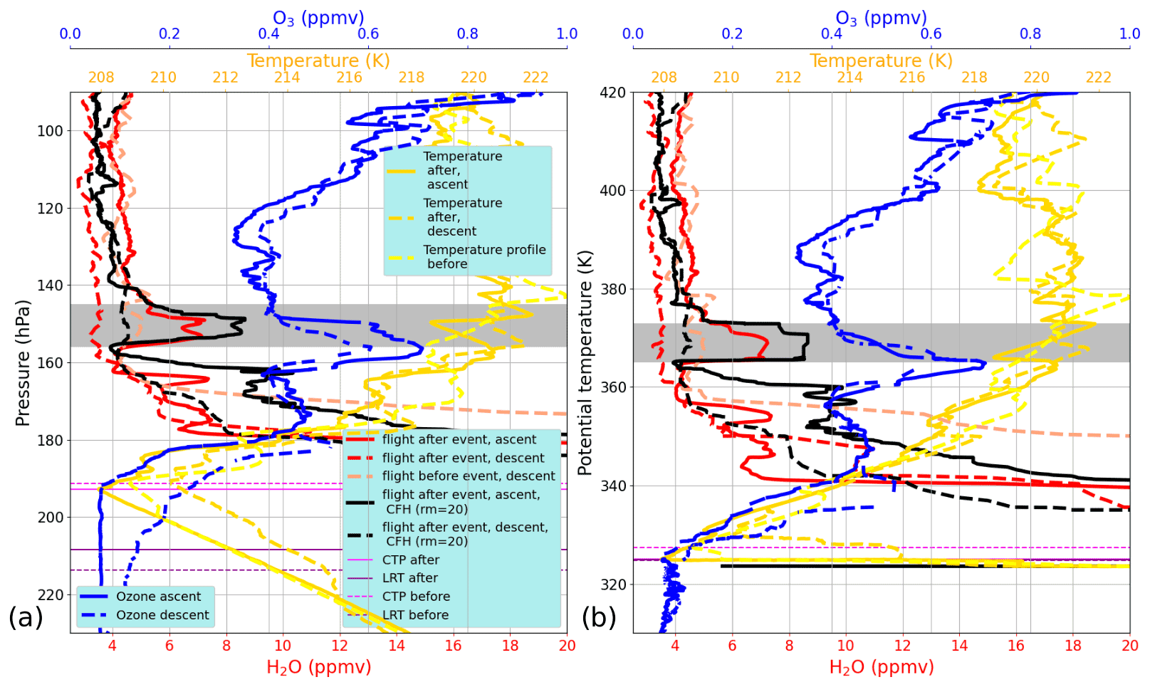
Figure 3Profiles measured immediately before and after the convective event (case 1) at 18:00 UTC, on 10 June 2019, and at 00:00 UTC, on 11 June 2019, in the UTLS region. The water vapor measurements are shown in reddish colors for the RS41 and in black for the CFH instrument. Ozone measurements are depicted in blue. Temperature is shown in yellowish colors. (a) Pressure is used as a vertical coordinate. (b) Potential temperature is used as a vertical coordinate. The different tropopauses (LRT and CPT) are shown as horizontal lines. The gray regions mark the level between 145 and 165 hPa in panel (a) and between 365 and 370 K in panel (b) at which the water vapor enhancement is observed.
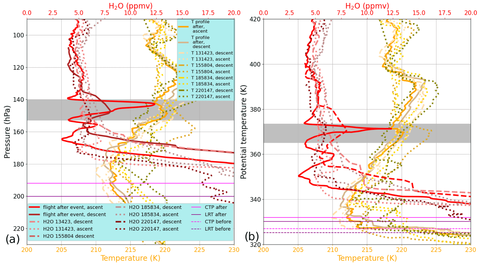
Figure 4Same as Fig. 3 but for profiles measured immediately before and after the convective event on 11 June 2019 (case 2) that passed the measurement site in the UTLS region. The water vapor mixing ratios are shown in red and were measured by the radiosonde before and after the event. (a) Pressure is used as a vertical coordinate. (b) Potential temperature is used as a vertical coordinate.
3.3 Source of the ozone peak at 150 hPa
Figure 3a shows the profile measured after the event of case 1. A strong ozone peak with values of up to 696 ppbv (parts per billion by volume) can be seen starting somewhat below the water vapor peak at a pressure level of 150 hPa. Usually, it is expected to find a negative correlation between water vapor and ozone when tropospheric air masses are injected by overshooting convection into the stratosphere. It is, therefore, unexpected to find such a strong increase (about 300 ppbv) in ozone at the same level as the water vapor injection. Figure 3b shows a steep decrease in ozone mixing ratios at potential temperature levels between 365 and 375 K. This indicates a dilution of the ozone-rich stratospheric air with ozone-poor tropospheric air. However, the origin of the ozone peak between the 160 and 375 K potential temperature level has to be clarified. Multiple possible explanations might be considered. One suggestion linked a strong increase in ozone to the injection of increased NOx produced by severe lightning (Seinfeld and Pandis, 2016; Bond et al., 2001; Cooray et al., 2009). NOx is controlling the O3 concentration in the troposphere and is mainly responsible for the development of photochemical smog in the troposphere. However, the increase of ≈ 300 ppbv cannot be explained by that because model simulations show that the potential increase due to NOx would be of the order of 10 ppbv (DeCaria et al., 2005).
Another ozone source can be direct corona discharge during lightning, leading to ozone formation (Minschwaner et al., 2008; Bozem et al., 2014; Kotsakis et al., 2017). However, the enhancement of ozone due to this process is reported to be of the order of about 50 ppbv and, thus, cannot explain the increase in the observed range. Figure 5a shows the ozone profile measured after the event during case 1 in comparison to the mean of all ozone profiles (eight available profiles) with multiple balloon measurements in Germany during spring- and summertime measurements between 2018 and 2020. It is evident that, although the profile of case 1 clearly exceeds the mean ozone profile at this altitude, it is not out of our observed range analyzed here. Figure 5b displays the H2O–O3 distribution of the same data as in Fig. 5a. Here, the data from case 1 (red dots), with the high amount of ozone and water vapor, diverge prominently from the typical L-shaped data set (gray dotted data) which marks the tropospheric and stratospheric regimes. It is not unusual that vertically thin filaments of ozone-rich stratospheric air masses are transported horizontally, causing local ozone enhancements in vertical profiles. A model run with CLaMS, using two different ECMWF reanalysis sets as input, shows an enhancement of ozone between 100 and 200 hPa (not shown). This indicates the horizontal transport of ozone-rich stratospheric air, as the CLaMS model does not account for overshooting events. Figure 6 presents the ERA5 reanalysis at the time and approximate altitude of the observed ozone peak. A narrow ozone-rich filament extends eastward from air masses with stratospheric origin towards the measurement location. Hence, there is strong evidence that the ozone-rich stratospheric filament was transported horizontally to the location where water vapor was injected by overshooting convection into the lowermost stratosphere. The location and development of the overshooting convection is discussed in Sect. 3.4 and 3.5.
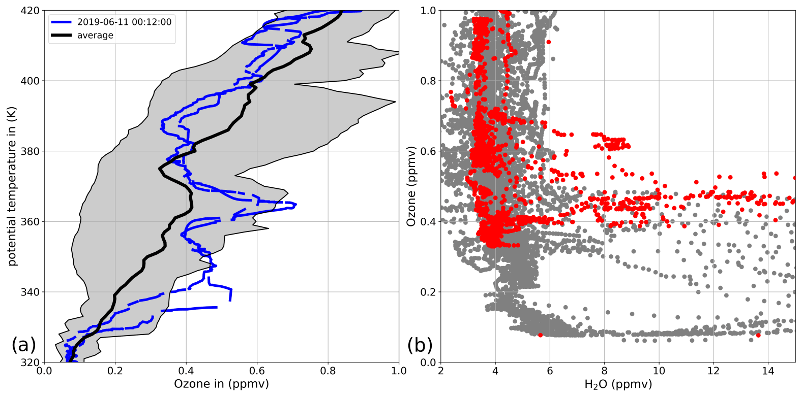
Figure 5Climatology of eight ozone profiles measured during spring and summer 2018–2020. (a) Ozone profiles, within the UTLS altitude range from 2018 to 2020, launched in the mid-latitudes in potential temperature coordinates. The shaded area marks the measured range of the ozone mixing ratios. The blue line shows ascent and descent data from the from case 1. (b) Tracer–tracer correlation of water vapor and ozone mixing ratios within the UTLS altitude range for the data obtained from 2018 to 2020 in the mid-latitudes. The red dots show the data from the ascent and descent from case 1.
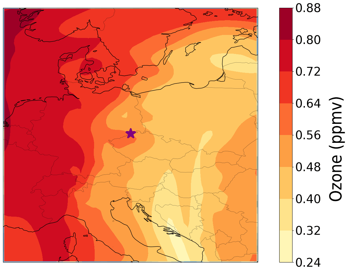
Figure 6Horizontal map of ERA5 ozone mixing ratio at a pressure level of 148 hPa on 11 June 2019 at 01:00 UTC (case 1). The measurement site is indicated by a purple star.
3.4 Comparison to the ERA5 reanalysis
ERA5 is used to place the measured data in a wider context and to evaluate the events. While ERA-Interim does not show any local signatures of the measured convection, the ERA5 reanalysis reveals the signature of a convective overshooting with multiple parameters. Here we consider CAPE, PV, potential temperature, and the water vapor mixing ratio, starting at midnight on 10 June 2019 until midnight on 14 June 2019. CAPE is the integrated amount of energy that the upward buoyancy force would act on a air parcel if it moves vertically. High CAPE values above 1000 J kg−1 show an increased probability of strong convective storm development in the case that convection is initiated. Figures 7a–c and 8a–c display the distribution of CAPE at three chosen points in time across Central Europe for cases 1 and 2 respectively. The white line marks the backward and forward trajectories which were initiated at the time and location of the measured water vapor peak for case 1 (discussed in Sect. 3.5), and the black dot marks the location of the sampled air mass at the given time point, according to the calculated trajectories. Very high CAPE values at the coast of Slovenia and Croatia as well, as the east coast of Italy and northern Italy, are evident in all chosen time frames.
Figure 7a–b show that the air mass measured after the event of case 1 is located just above a strong maximum in CAPE over north Italy on the morning of 10 June 2019. Throughout the day, the air parcel moves close into regions of enhanced CAPE on multiple occasions along the way to the measurement site, and finally reaching the center of a region with high CAPE close to the measurement site (Fig. 7c). Figure 8a–c depict the same scenario for case 2. Here, the air masses crosses a location with high CAPE for the first time at 06:00 UTC on 11 June 2019 over Slovenia. It remains within the region of high CAPE until 13:00 UTC before it crosses the measurement site at midnight.
In contrast to the persistent and wide-ranged horizontal distribution of elevated CAPE values, a different structural evolution is observed in the PV (not shown) and dTheta. When considering dTheta at the altitude of the measured air parcel with enhanced water vapor, a strong minimum can be seen, which coincides with the signature of PV for cases 1 and 2. For case 1, on the day before the measured event, no profound signature in the dTheta structure is seen until 09:00 UTC on the morning of 10 June 2019 (Fig. 7d). However, at 10:00 UTC (Fig. 7e), a spot signature in dTheta is apparent, leading to PV values of up to 25 PVU in the region of high CAPE values over northern Italy. This is more than twice as high as the surrounding PV values. The air mass later sampled is located at the edge of the strong dTheta enhancement with still strong values remaining throughout the next 10 h. This signature subsequently weakens (Fig. 7e) but reappears with increased intensity (Fig. 7f) and moves northwards until it dissolves at midnight. The trajectory of the air parcel moves only slightly westward of this structure but remains inside the enhancement of PV over the entire time, although never in the center.
A similar course of events can be observed for case 2, as shown in Fig. 8. In comparison to case 1, the trajectory of the air mass measured in case 2 approaches further from the south. In the early morning hours of 11 June 2019, no significant structure or signal can be seen in the area of interest (Fig. 8d). At 10:00 UTC a dipole structure in dTheta appears, leading to PV values of up to 30 PVU (Fig. 8e). Similar to case 1, the signal neither develops gradually nor is it transported horizontally into the considered area and instead emerges on a very short timescale. The anomaly appears over Austria, northern Italy, and over the Czech Republic and, therefore, has three central points. The enhancement over the Czech Republic dissolves in the following hour, while the other two increase in strength over the next few hours. However, all three centers dissolve until midnight when the air parcel reaches the measurement site. In case 2, the air parcel is also constantly in the vicinity of at least one of the peaks in dTheta but never enters areas of the extraordinary high values.
This signature in dTheta can be explained with the displacement of the isentropes upward by strong updraft winds and local diabatic heating, which cause an increase in the gradient of potential temperature, as has been shown by Qu et al. (2020). In both cases considered here, the map of the dTheta is homogeneous before convection appears until 09:00 UTC (Fig. 7g–i). However, only 1 h later, a spot signal with values of up to −2.7 K hPa−1 appears, which is more than 3 times higher than the surrounding values. In both cases, the peak in dTheta moves along the PV enhancement and also dissolves at the same time.
Furthermore, the specific humidity in ERA5 was analyzed. Figure 7g–i show the specific humidity of ERA5 for case 1. Figure 7g shows the hour before the first appearance of the signature of the convective storm for case 1 at 09:00 UTC on 10 June 2019. In total, two peaks can be seen on the map but not close to the path of the air mass. Then, 1 h later, at 10:00 UTC, a water vapor peak emerges in the vicinity of the air mass (Fig. 7h) at the same location as the enhancement in PV and dTheta. For case 2, a similar picture is seen. While no local enhancements in water vapor mixing ratios can be seen in the considered area at 09:00 UTC, only 1 h later, at 10:00 UTC, a strong enhancement in water vapor is evident in the vicinity of the considered air mass. This signature of the local enhancement is almost twice as high as the peak seen for case 1. Similar to case 1, the enhancement is transported towards the measurement site throughout the day and remains close to the measured air mass.
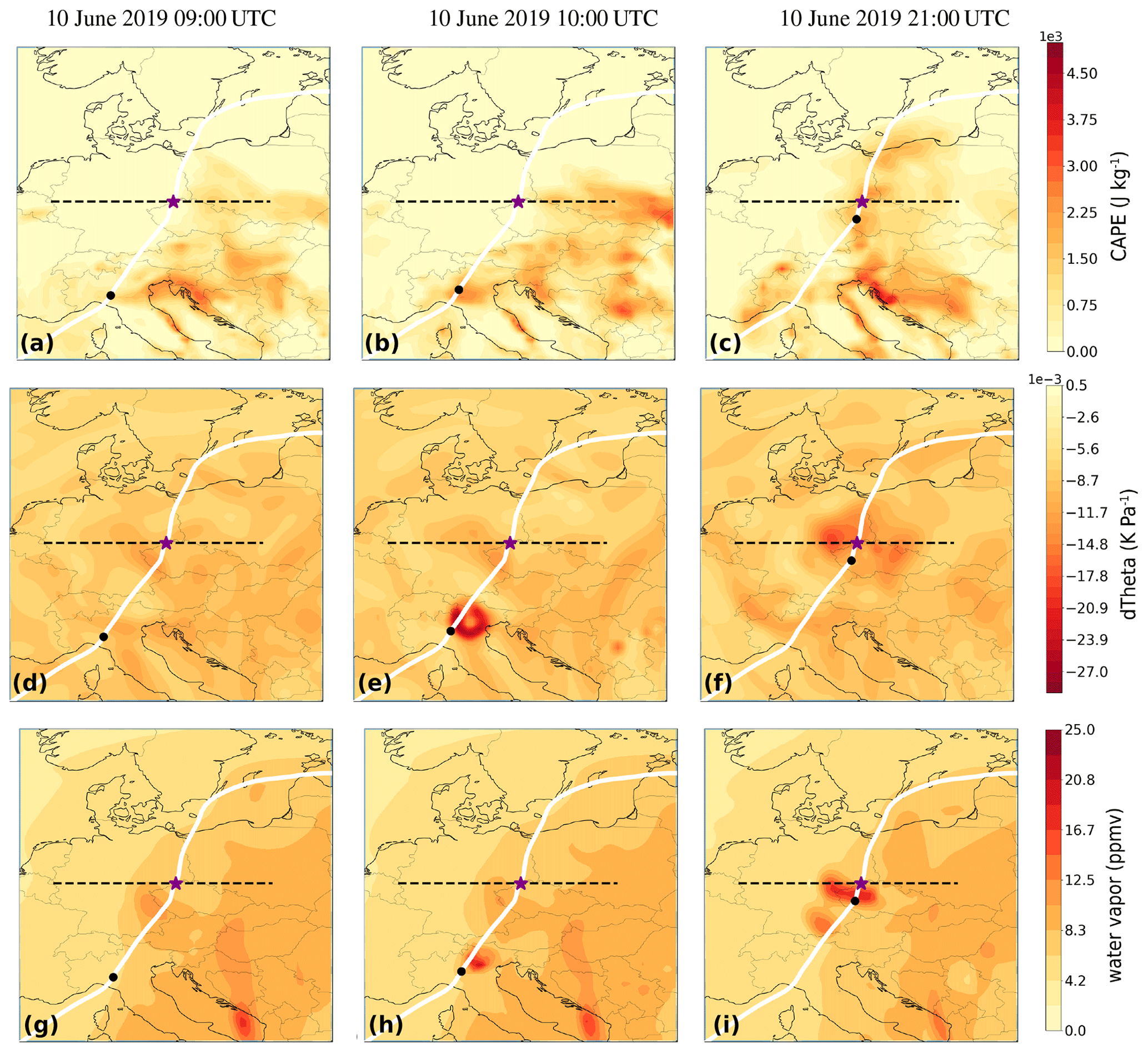
Figure 7CAPE from ERA5 (a–c) vertical gradient of potential temperature (dTheta; d–f), and specific humidity (g–i) at three chosen time points for case 1 (09:00, 10:00, and 21:00 UTC on 10 June 2019). dTheta and specific humidity are displayed at a pressure level of 148 hPa. The horizontal black dashed line denotes the latitude of the measurement site, and the purple star indicates the exact measurement location. The white line shows the trajectory of the measured air parcel, as described in Sect. 2.4. The black dot on the trajectory line represents the calculated location of the air mass at the given point in time.

Figure 8The same as in Fig. 7 but for case 2 with three chosen points in time (09:00, 10:00, and 18:00 UTC on 11 June 2019).
3.5 Origin and evolution of the water vapor enhancement along the CLaMS trajectories
In order to determine the origin and evolution of the measured air masses containing the water vapor enhancement, 100 h backward and 100 h forward trajectories were calculated for both cases, as described in Sect. 2.4. The backward trajectories are not shown before 06:00 UTC on 9 June 2019, as the points do not contain any relevant information related to the measurements. Figure 9a displays the water vapor mixing ratios along the trajectory and the data points measured by MLS within 5∘ of latitude and longitude and an hour before or after the trajectory point (star symbols). The ERA5 water vapor mixing ratio shows a sharp increase along the trajectory, from values around 7 ppmv to values up to 15 ppmv, ≈ 10 h before the balloon measurement took place. Figure 9b shows the mixing ratios of ozone and water vapor, as well as PV and CAPE values from ERA5, along the trajectory. The trajectory encounters high CAPE values shortly before a steep increase in water vapor and PV appears on 10 June 2019 at around 10:00 UTC. The peak in CAPE is followed by a peak in PV almost doubling the preceding values of around 8 PVU. This peak is in good agreement with an increase in water vapor mixing ratios by 10 ppmv, which remains at the level between 12.3 and 17.5 ppmv throughout the following 4 d of the trajectory (in contrast to the PV enhancement which decreases shortly before the balloon observations to a background value of 8 PVU). With a water vapor mixing ratio of 10 ppmv measured by the CFH at the peak, the values obtained with the balloon payload are lower than the ERA5 values. The ozone mixing ratios do not show an impact by the convective event but steadily decrease throughout the trajectory. Figure 9c shows MLS water vapor, ozone, and CO mean mixing ratios for the nearest MLS point for each time step within 300 km along the trajectory. Only seven measurement points were found to match the criteria. Although multiple MLS data points were available, a clear increase in water vapor cannot be seen in the available data. Overall, the values measured by MLS are much lower compared to the ERA5 water vapor values, which range from 2 to 6 ppmv along the calculated trajectory, while the ERA5 values vary between 5 and 18 ppmv. CO and water vapor act as a tropospheric tracer, with sources at the surface and background values in the stratosphere (Ricaud et al., 2007), and were considered here as a potential additional tracer for convective overshooting. The nearest values of the individual data sets do not show any increase in relation to the proposed convective event. This emphasizes the small scale of the overshooting event and the local scale of the water vapor enhancement, as MLS only has a very coarse spatial resolution in the LS. While the vertical extent of the water vapor peak is 800 m (600 m for case 2), the vertical resolution of MLS H2O measurement is 1.5 km.

Figure 9Trajectory of the measured air mass for case 1, with MLS data taken within 5∘ of latitude and longitude of the trajectory. Panel (a) shows the trajectory on a map, with the color-coded water vapor mixing ratios along the trajectory. Additionally, all MLS data points within a longitude and latitude of 5∘, as well as within 1 h before and after the individual trajectory points, are shown as star symbols. In panel (b), the water vapor from ERA5 along the trajectory is displayed in red, ozone in blue, PV in black, and CAPE in orange. The time of the measurement and the observed maximum water vapor mixing ratio from CFH and RS41 within the pressure levels of 145 and 165 hPa are shown at the vertical blue line and with blue and red symbols, respectively. Panel (c) displays the same time frame, with the nearest MLS measurements of ozone in blue, water vapor in red, and CO in purple, within a radius of 300 km of each trajectory point and 1 h before or after the trajectory point.
A similar picture appears for case 2, as shown in Fig. 10. It must be noted that the scales differ in comparison to Fig. 9. In case 2, at midday on 10 June 2019, a series of peaks in CAPE emerge and persist throughout the next 4 d. Shortly before the start of these variations in CAPE, a slight increase in PV is evident, and PV values subsequently show enhanced values, although not exceeding 9.5 PVU at a background of 7.5 PVU. Water vapor along the trajectory remains constant until midday on 11 June 2019, when it is slightly enhanced from approximately 6 to 10 ppmv shortly after CAPE and PV reach maximum values ≈ 11 h before the measurement took place. Similar to case 1, the water vapor continuously remained at the elevated mixing ratios throughout the end of the trajectory. For case 2, only four MLS measurement points were found within 300 km of the trajectory. A slight enhancement of 1 ppmv in the water vapor mixing ratio in the MLS data after the overshooting convection and a 30 ppmv increase in CO, which remains enhanced between 55 and 65 ppmv, together with a slight decrease in ozone mixing ratio by 20 ppbv can be seen. Here it is emphasized that the overshooting event of case 2 likely has a wider horizontal extent, which makes it more suitable for detection by the MLS instrument. This is supported by the fact that, in contrast to case 1, both the ascending and descending profiles show enhancements of tropospheric air in the lower stratosphere. The trajectories for the two cases show an increase in the water vapor before the air parcel arrived at the measurement site. The increase in water vapor is accompanied by an increase in PV and high CAPE values. While in case 1 the steadily decreasing ozone values along the trajectory seem to be unrelated to the changes in the other trace gases, in case 2, an increase in ozone mixing ratios by 150 ppbv occurs at the same time as the increase in the PV values. In contrast to case 1, where the peak in PV initially decreases shortly before reaching the measurement site and returns to background values 1 d later, in case 2 the PV values keep increasing but never reach the high values of case 1. In both cases, the water vapor mixing ratios remain enhanced after the overshooting convection in the model and shortly before reaching the measurement site. However, case 2 shows lower values at around 10 ppmv in comparison to 15 ppmv for case 1. With these values, the ERA5 water vapor value is greater than the measured value in case 1 but is slightly below the values measured in case 2.
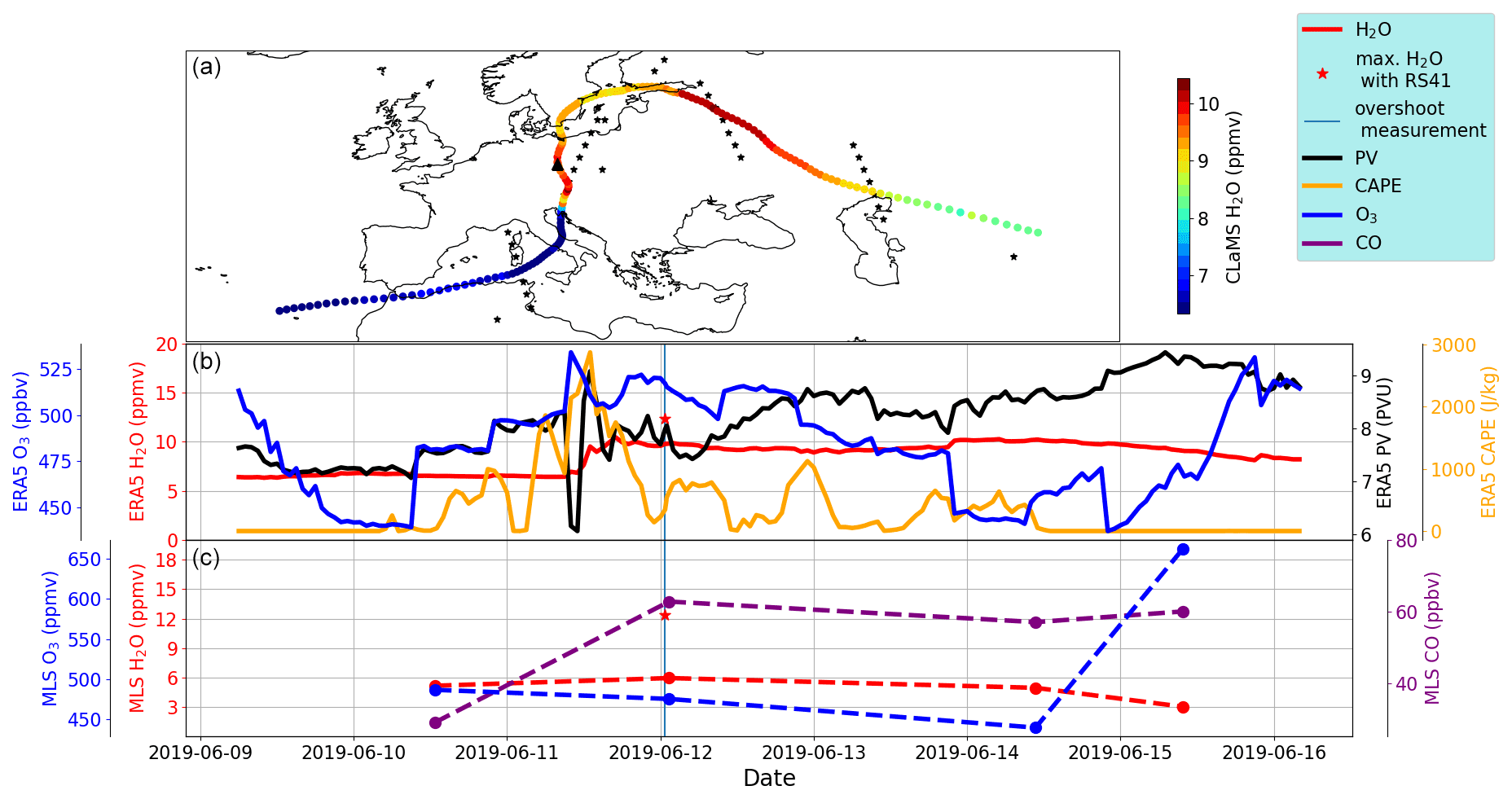
Figure 10Same as in Fig. 9 but for case 2. The time of the measurement is marked with a vertical blue line, and the observed maximum water vapor mixing ratio from RS41, within the pressure levels of 139 and 155 hPa, is shown with red star in each panel.
3.6 Overshooting events in satellite data
The satellite measurements of brightness temperature (BT) from geostationary Meteosat-10 rapid scan data support the above-indicated tropospheric origin of the measured water vapor enhancement in the lower stratosphere. Figure 11a–d show Meteosat-10 BT data for two chosen times in case 1. Figure 11a shows the data at 05:29 UTC on 10 June 2019. A cloud structure reaching a BT as low as 205 K surrounds the air mass along the trajectory at this time. For case 1, a CPT of 208 K was measured and confirmed by the surrounding cloud-top BT between 210 and 216 K. It is, therefore, most likely that areas with a BT below 205 K resemble areas of overshooting tops. These areas are circled in pink in Fig. 11. In addition to the trajectories discussed in Sect. 3.5, further trajectories were calculated starting at the same location but at lower pressure levels, as both balloon profiles not only exhibited a main peak at a pressure level of 149 or 144 hPa but also covered an underlying water vapor enhancement at 165 or 155 hPa, respectively, for cases 1 and 2 (Figs. 3 and 4). Trajectories initialized at 149, 155, and 165 hPa and at 144, 153, and 155 hPa, respectively, for case 1 and case 2 were calculated and added to the satellite image. The air mass on the trajectory starting at 149 hPa is located closest (only 50 km northeast) to the coldest and, therefore, highest point of the convective cloud, as can be seen in detail in Fig. 11a. Considering the slight uncertainties in the trajectory calculation and in the meteorological fields, this point in time is most likely responsible for the water vapor enhancement detected later. However, the satellite images display the coinciding of the air mass and the convective event 4 h earlier compared to ERA5 and, therefore, further southwest. Later in the day, the air mass location coincides with another overshooting cloud at around 21:09 UTC (see Fig. 11b). Multiple areas exceed the tropopause height in the convective clouds but none of the air masses on the trajectories seem to be very close to these areas.
The trajectories for case 2 pass by near to the convective events as well; however, these are at a greater distance from the overshooting tops (Fig. 12a and b). For case 2, Fig. 4b shows a temperature of 214 K at the tropopause height. Trajectories initialized at pressure levels of 145, 150, and 155 hPa can be seen in Fig. 12 and encounter the cloud-top height with temperatures 6 K below the tropopause temperature. Similar to case 1, in case 2, an additional convective storm develops over eastern Germany with overshooting tops. However, the air masses along the trajectories do not encounter this convective cloud (see Fig. 12a and b). Thus, it is very likely that the observed water vapor enhancement resulted from the overshooting event that occurred over Austria on 11 June 2019 at around 14:24 or 15:49 UTC.

Figure 11Brightness temperatures from geostationary Meteosat-10 satellite using the IR 10.8 µm channel along trajectories for case 1 during two different times (a at 05:59 UTC and b at 21:09 UTC on 10 June 2019). Air mass trajectories initiated at different pressure levels (149, 155, and 165 hPa) are shown with gray to black lines. Air masses with BT < 205 K are depicted with pink contours.
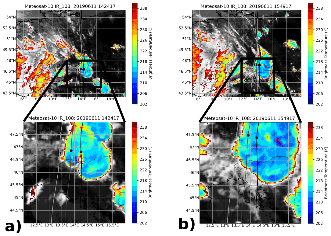
Figure 12Same as Fig. 11 but for case 2. Air mass trajectories initiated at different pressure levels (144, 153, and 155 hPa) are shown with gray to black lines. Air masses with BT < 209 K are denoted with pink contours. Panel (a) shows the satellite image at 14:24 UTC and panel (b) at 15:49 UTC on 11 June 2019.
The measurements presented here show a strong enhancement in water vapor above the tropopause on 2 consecutive days, i.e., 10 and 11 June 2019. Both cases originate from gravity waves breaking behind the overshooting top, leading to in-mixing of tropospheric air into the lower stratosphere several hours before the balloon launch.
The water vapor mixing ratio enhancement measured in case 1 is located 40 K above the thermal tropopause when using potential temperature as a vertical coordinate. This is comparable to a study by Smith et al. (2017), where water vapor mixing ratio enhancements were measured during multiple airborne missions above the North American continent. Smith et al. (2017) use 370 K as a typical tropopause altitude and discuss water vapor enhancements at a level between 400 and 410 K, with values up to 6 ppmv above the background values. Similarly, the water vapor values measured in case 2 are of the same order of magnitude. The maximum of the peak is approximately 40 K above the tropopause potential temperature and reaches 7.5 ppmv above the background value. The same order of magnitude was observed during the SEAC4RS aircraft measurement campaign, with elevated water vapor mixing ratios of up to 10.6 ppmv in the lowermost stratosphere at ≈ 100 hPa (Robrecht et al., 2019).
The local injection of water vapor was detected within a larger-scale peak in ozone for case 1. This peak results from a horizontal transport of stratospheric air masses with a strong stratospheric signature from west to east. An edge of a filament from a front with high ozone values is stretched over the measurement location. A map of ERA5 ozone at 145 hPa, as given in Fig. 6, shows that the balloon measurement was at the edge of a front with higher ozone mixing ratios. This explains the lower ozone values at the same pressure or potential temperature level in the descending profile which was located further north. This is also supported by the sparse data from MLS, which show higher ozone mixing ratio values westward of the measurement site and lower values of about 200 ppbv east of the measurement site (see Fig. 9). The ERA5 ozone values along the calculated trajectory of the measured air mass further support this assessment. The moistening of the ozone-rich air mass lead to an unusual feature in the tracer–tracer correlation, as shown in Fig. 5b.
Case 1 not only shows a strong enhancement of water vapor mixing ratios in the ascending profile of the balloon-borne measurement, but further expected indications of a tropospheric air injection were also recorded. A sharp decrease in ozone mixing ratios occurs at the same potential temperature level as the rise in water vapor. The drop in temperature is equally sharp and aligned with the change in water vapor and ozone, albeit less prominent. The elevated water vapor, decrease in ozone mixing ratios, and lower temperatures all indicate the tropospheric origin of the measured air mass between the potential temperature levels of 365 and 375 K. The air mass is clearly different from the air masses above and below to a degree that the profile of the water vapor peak appears to be square shaped (see Fig. 3b). The fresh in-mixing and the tropospheric origin of the air masses is also underlined by the small spatial extent of the enhancement. This is derived from the following two observations: first, the balloon measurement does not show any enhancement of water vapor in the descending profile, and second, no clear trace of the event can be found in the MLS measurements due to the low vertical and horizontal (cross-track) resolution at the limb tangent point of 1.5 and 3 km, respectively. The tropospheric source of the water vapor injection for case 1 is supported by satellite BT measurements of overshooting tops and by ERA5 displaying a local disturbance in PV and dTheta along the trajectory of the discussed air mass. The dTheta anomaly is in good agreement with the local enhanced water vapor mixing ratio in ERA5 (Fig. 7d–f). The BT satellite data suggest that this coinciding of the measured air mass and the convective overshooting event occurs ≈ 4 h earlier at 05:29:18 UTC further southwest, but otherwise both the reanalysis and the observational data show a convective storm moving northwards, with high-reaching cloud tops and BTs reaching as low as 205 K. Until this convective event dissolves after 22:00 UTC, the measured air parcel remains close to its center. The air mass along the trajectory starting at 149 hPa encounters a second, stronger, and more spatially distributed convective event over the northeast of Munich (southeastern Germany), in the evening at 18:19 and 19:39 UTC, where it also passes close to a cloud-top height reaching 202 K BT (see Fig. A2). The air masses continue to remain in this growing convective cloud, which eventually covers the entirety of eastern Germany, until the measurement site is reached. As described in Smith et al. (2017), Qu et al. (2020), and Dauhut et al. (2018), the in-mixing of tropospheric air masses is caused by gravity waves breaking closely behind an overshooting top into the surrounding stratospheric air, which has a lower water vapor mixing ratio and a higher potential temperature. The hydrometeors from the injection sublimate and are mixed into the stratospheric air mass on very small timescales under these strongly subsaturated conditions. It is, therefore, consistent that the additional COBALD measurement (not shown) did not detect any cloud particles in the measured profile. Additionally, the sublimating hydrometeors cool the air mass. It is very likely that the air mass descended slightly due to the decreased potential temperature after the mixing of tropospheric and stratospheric air and, therefore, reached neutral buoyancy at a lower level than was later found in the balloon profiles. This process would not be evident in the calculated trajectories and, thus, slightly increases the inaccuracy of the presented trajectories. However, the descent of the air mass due to the adjustment of potential temperature is expected to be rather low due to the very humid conditions of the LS mixed-in tropospheric air mass. Furthermore, the existence of sublimated hydrometeors in the entrained air masses result in a relatively low amount of air that is ultimately irreversibly mixed within the LS.
Case 2 shows a similar signature but differs in several aspects. First, the balloon profile measurements in Fig. 4a and b show that the water vapor enhancement is stronger and is located at a lower pressure level (although the level of potential temperature remains almost the same). In contrast to case 1, only radiosonde measurements are available for case 2, and thus, only water vapor data measured by the radiosondes can be compared for both cases. While in case 1 the peak value is 7.0 ppmv, in case 2 the maximum peak value reaches up to 12.1 ppmv. In addition, balloon measurements for case 2 potentially indicate not only a stronger but also a spatially larger event, as the descending profile reveals a peak in water vapor that still reaches more than 7.5 ppmv but with a wider vertical spread. This indication is supported by the MLS measurements. For case 2, a slight increase in MLS water vapor mixing ratios (≈ 1 ppmv) is visible after the balloon observation compared to the MLS data point that was taken before the suggested convective event (see Fig. 10). The development of the water vapor peak does not form a square shape when using potential temperature as a vertical coordinate and instead forms a sharp tip after a steep water vapor increase. Slightly below this tip, a drop in temperature can be seen (Fig. 4b), with a similar decrease (by about 2 K) to that of case 1. A further difference between the cases is the tropopause. While case 1 shows a very sharp tropopause, case 2 has a rather flat tropopause with an inversion layer at 125 hPa. In the temperature profile obtained 2 h prior to the profile with enhanced water vapor (displayed in Fig. 4a and b), a second tropopause is detected. Throughout the day of case 2 (launched at 13:11 and 22:00 UTC on 11 June 2019), two profiles with double tropopause were measured, which indicates a less stable atmospheric profile and possibly supports the findings of Solomon et al. (2016), who found that the overshooting convection is more likely in cases of a present double tropopause.
ERA5 also shows a difference between the two cases. Case 2 shows a higher and wider spread of CAPE values before the overshooting event throughout the day when compared to case 1. The PV anomaly discussed in Sect. 3.4 shows a cluster of individual anomalies around the calculated trajectory instead of a single event, as in case 1. According to the satellite data, the air mass measured in case 2 encounters a convective event once in the afternoon over Austria (see Sect. 3.6) but does not encounter a second event later, which is in contrast to case 1. While ERA5 shows a likely overshooting event for case 1 4 h before, and slightly northwest of the event observed by satellites, the convective event in ERA5 for case 2 is 4 h later than the satellite observation.
Overall, the ERA5 data indicates that the measured air parcels of both cases were moistened by the occurrence of an overshooting convective storm, which caused a local nonconservative PV anomaly to appear at the level of the measured air parcel. This PV signal was most likely caused by the upward displacement and narrowing of the isentropes in combination with diabatic processes and related small-scale mixing (Qu et al., 2020). The overshooting convection which moistened the measured air parcel in the lower stratosphere occurred in the north of Italy several hours before the convective event arrived at the measurement site, as implied by satellite data and ERA5. However, the moistened air parcels took a similar pathway in the lower stratosphere to the convection in the troposphere before both arrived at the measurement site in eastern Germany. It is not clear from the data whether the air parcel was moistened once during the first appearance of the convective storm in the northern part of Italy or if it was moistened multiple times along the trajectory, as indicated by the satellite images over Bavaria to the south of the measurement site. In addition, the question as to when exactly water vapor was injected into the lower stratosphere remains unanswered. However, it is evident that the water vapor was injected into the lower stratosphere by convective overshooting and is not caused by another mechanism, such as, for example, the horizontal transport and the in-mixing of tropical air masses at the subtropical jet.
Overshooting convective events are known to inject water vapor into the lower stratosphere. However, their quantitative impact on the variability in water vapor mixing ratios in the mid-latitudes requires further investigation. A number of case studies of overshooting tops and their vertical transport of water vapor were performed above the North American continent. However, in situ measurements over Europe are still sparse. In this study, two cases of water vapor injection into the lower stratosphere over the German–Czech border are presented. The balloon-borne in situ measurements show water vapor enhancements in excess of the background value of 5 by 3.65 ppmv for case 1 and 7.1 ppmv for case 2. Both cases show clear evidence for overshooting convection and have a comparable scale to overshooting events measured in previous studies over the North American continent. The findings of the in situ balloon-borne measurements are supported by ERA5 and by satellite data. We emphasize here that ERA5 includes the overshooting convection and moistening of the LS in both cases, which is in contrast to ERA-Interim reanalysis. The location and timing of the observation was not precisely matched by ERA5 but was, nevertheless, relatively close to the event observed in the satellite data. It is shown that the measured enhancements of water vapor at a pressure level of 149 and 144 hPa, respectively, for cases 1 and 2 were injected into the lower stratosphere several hours before the measurement took place and were horizontally transported to the measurement site. Stratospheric moistening through overshooting convection over the North American continent has already been reported (Smith et al., 2017). Here we report evidence demonstrating that stratospheric moistening also occurs by overshooting convection over Europe. The strength of the measured water vapor enhancement shows that the role of overshooting convection over Europe and in mid-latitudes in general, as a contributor to the lower stratospheric water vapor budget, might be underestimated due to the sparse in situ data. As it is expected that the frequency and strength of extreme convective events will increase with advancing global climate change, it is crucial to thoroughly understand and quantify the impact of these events. MLS satellite measurements are not always suitable for detecting these small-scale water vapor enhancements, as shown especially in one of the two cases. Thus, studies estimating the relevance of overshooting convection on the extratropical water vapor distribution using satellite data might underestimate their effect in general and not only over Europe. Therefore, because of the low resolution of satellite data, in situ measurements and future satellite missions with very high vertical resolution in the UTLS are therefore required to understand the impact of such small-scale events like overshooting convection.
A1 Electrochemical concentration cell (ECC)
Electrochemical concentration cells (ECCs) are lightweight in situ ozonesondes that have been used for multiple decades on weather balloons to investigate ozone mixing ratio profiles and to monitor long-term ozone trends, e.g., in the Southern Hemisphere within the SHADOZ network (Southern Hemisphere ADditional OZonesondes; Thompson et al., 2019). The ambient air is pumped through a Teflon tube into the reaction cell at a speed of about 29 s/100 mL at ground conditions. In the reaction cell of the device, a chemical reaction of the ambient ozone with potassium iodide produces two electrons for each ozone molecule. The resulting current is, thus, proportional to the partial pressure of ozone in the sampled air. Komhyr et al. (1995) describe the ECC in detail. In order to gain high-quality data, the exact composition of the potassium iodide solution is crucial. Johnson et al. (2002) present an extended study of different solution variations and their effect on the background current. In this study, we use a solution composition of 1 % and (one-tenth) buffer suggested by Johnson et al. (2002) for the most accurate ozone data, which is in contrast to the long-term measurement series that consistently uses one solution combination suggested by Komhyr et al. (1995) and Smit et al. (2007). For the analysis of the data, the methods, i.e., time lag correction and background current correction, described by Vömel et al. (2020) are used.
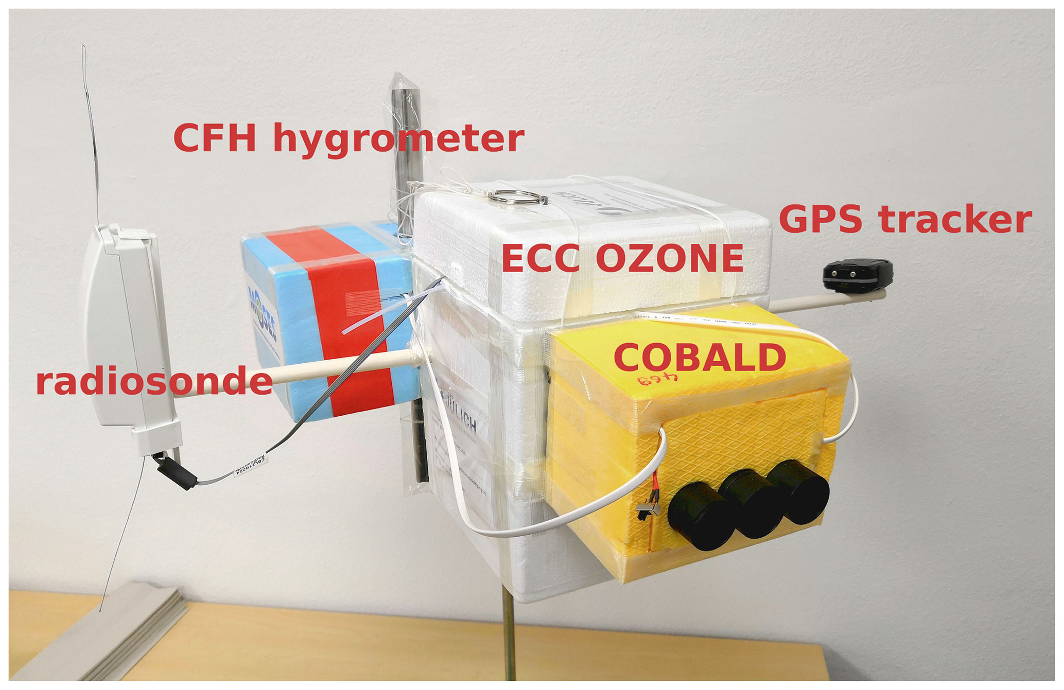
Figure A1Combined full balloon payload. The ECC is located in the white styrofoam box, the COBALD is in the yellow box, and the CFH is embedded in the light blue box. A white wooden stick goes through the ozone box and has the radiosonde attached on one side, while an independent GPS tracker is attached on the other to locate the payload after the landing. In total, the payload has a mass of 2.6 kg. The payload is attached to an unwinder, which ensures that the balloon launch takes place smoothly despite the 60 m of string between the balloon and payload. The unwinder is connected to a parachute to reduce the falling speed of the payload after the balloon bursts and assures a safe landing. The parachute is connected to the 1500 g balloon.
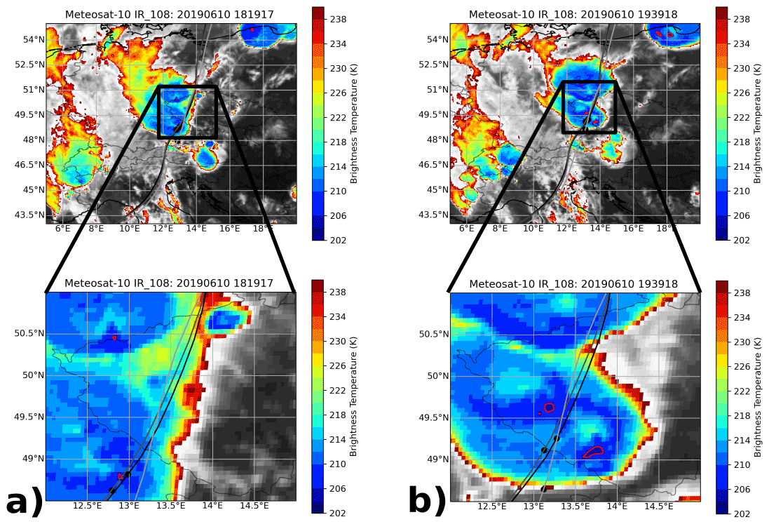
Figure A2Same as Fig. 11 but for a different point in time. Air mass trajectories initiated at different pressure levels (144, 153, and 155 hPa) are shown with gray to black lines. Air masses with BT < 209 K are marked with pink contours. Panels (a) and (c) show the satellite image at 18:19 UTC and panels (b) and (d) at 19:39 UTC on 10 June 2019.
A2 Cryogenic frost point hygrometer (CFH)
The cryogenic frost point hygrometer (CFH) is a balloon-borne instrument based on the cold mirror principle, which regulates the temperature of a mirror to the frost point temperature of the ambient air (Vömel et al., 2007). The mirror is constantly cooled with a cooling agent, R-23 (trifluoromethane), and a feedback loop regulates the temperature of the mirror to be constantly coated with a thin layer of ice. Prior to the flight, the cooling agent is pre-cooled to liquid state at −86 ∘C and poured into the instrument. With decreasing ambient pressure during the flight, the temperature of the liquid decreases to −120 ∘C at tropopause level. When the mirror is covered with a thin layer of ice and is in a steady state, the mirror temperature is equal to the frost point temperature of the measured air mass. The thickness of the ice layer is controlled by the reflectivity of the mirror, which is measured by a light beam and a detector. As soon as the ice layer on the mirror becomes thicker, a smaller proportion of the light beam is reflected by the mirror. The detector then sends a signal to a heater to regulate the temperature of the mirror. This regulating cycle is constantly maintained, leading to a thermodynamical equilibrium between the ice layer and ambient air and resulting in a relatively low uncertainty of the instrument. The uncertainty of the instrument is defined by the stability of the feedback controller and is defined as 0.5 ∘C, which leads to a relative uncertainty below 4 % in the troposphere and below 10 % in the stratosphere (Vömel and Diaz, 2010; Vömel et al., 2016). Klanner et al. (2021) used the CFH in comparison with the water vapor lidar system and found a very good agreement within their respective uncertainties throughout the entire atmospheric profile. A potential failure of the instrument can be caused by liquid droplets on the detector, the mirror, or the light source. It is, therefore, recommended that the CFH is not launched during rain.
A3 Vaisala Radiosonde RS41
The Vaisala Radiosonde RS41 was introduced in 2014 and completely replaced the RS91 precursor model in 2017. The temperature sensor is based on resistive platinum technology. The manufacturer states that there is a combined uncertainty of 0.3 K below 16 km and of 0.4 K above. The response time of the temperature sensor is < 1 s and, thus, does not need to be considered in the following. The temperature range is given as −95 to 60 ∘C, and the resolution is 0.01 ∘C (Jauhiainen et al., 2014; Vaisala, 2020). The humidity sensor is a thin film capacitor. The combined uncertainty for the humidity sensor is given as 3 %, and the resolution is given as 0.1 % relative humidity. Similar to the temperature sensor, the response time of the humidity sensor is < 0.3 s at 20 ∘C and < 10 s at −40 ∘C. The pressure sensor is a silicon capacitor and is defined for a pressure range between surface pressure and 3 hPa, while the resolution is given as 0.01 hPa.
Dirksen et al. (2020) found in experimental work that the humidity sensor of the RS41 has an uncertainty of <1.5 % and a temperature uncertainty of <0.2 %. Survo et al. (2014) validated the uncertainty of the RS41 temperature and humidity data. No systematic drifts due to storage were found in either temperature or in humidity measurements. However, an increase in temperature uncertainty was found from 0.13 ∘C in the troposphere up to 0.3 ∘C at 30 km. An uncertainty below 1 % relative humidity was found in the stratosphere.
Balloon-borne data are available from http://www.tereno.net/geonetwork (Forschungszentrum Jülich IBG-3, 2022). MLS data can be downloaded at https://earthdata.nasa.gov/earth-observation-data/near-real-time/download-nrt-data/mls-nrt (for water vapour, see https://doi.org/10.5067/Aura/MLS/DATA2009, Lambert et al., 2015; for ozone, see https://doi.org/10.5067/Aura/MLS/DATA2017, Schwartz et al., 2015b; for CO, see https://doi.org/10.5067/Aura/MLS/DATA2005, Schwartz et al., 2015b). ECMWF ERA5 data are available at https://cds.climate.copernicus.eu/cdsapp#!/home (Copernicus Climate Change Service, 2017).
CR, DK, and AW performed the balloon-borne measurements and wrote the draft. CR and DK performed the data analysis from the balloon-borne data, the MLS data, and ERA5 reanalysis. CR performed the Meteosat-10 data analysis. Data interpretation of the ERA5 was performed by JUG, RM, PK, CR, and DK. All authors contributed to the data interpretation with scientific discussions and read and agreed to the published version of the paper.
At least one of the (co-)authors is a member of the editorial board of Atmospheric Chemistry and Physics. The peer-review process was guided by an independent editor, and the authors also have no other competing interests to declare.
Publisher’s note: Copernicus Publications remains neutral with regard to jurisdictional claims in published maps and institutional affiliations.
We would like to thank NASA and the MLS team, for providing the water vapor data from the Microwave Limb Sounder (MLS) on the Aura satellite. We would also like to thank EUMETSAT, for the Metop10 brightness temperature data. In addition, we are grateful to the ECMWF, for their meteorological reanalysis data support. A special thanks goes to the Karlsruhe KITcube Team, who always supported us during the MOSES measurement campaign.
The balloon activities were funded by the Helmholtz Association within the framework of MOSES (Modular Observation Solutions for Earth Systems).
The article processing charges for this open-access
publication were covered by the Forschungszentrum Jülich.
This paper was edited by Farahnaz Khosrawi and reviewed by Zhipeng Qu and one anonymous referee.
Anderson, J., Wilmouth, D., Smith, J., and Sayers, D.: UV Dosage levels in summer: increased risk of Ozone loss from convectivly injected water vapour, Science, 337, 835–839, https://doi.org/10.1126/science.1222978, 2012. a
Bond, D., Orville, E., and Boccippio, J.: NOx production by lightning over the continental data from are in accordance assuming a NO production rate molecules for each CG and produce than despite study, J. Geophys. Res., 106, 27701–27710, 2001. a
Bozem, H., Fischer, H., Gurk, C., Schiller, C. L., Parchatka, U., Koenigstedt, R., Stickler, A., Martinez, M., Harder, H., Kubistin, D., Williams, J., Eerdekens, G., and Lelieveld, J.: Influence of corona discharge on the ozone budget in the tropical free troposphere: a case study of deep convection during GABRIEL, Atmos. Chem. Phys., 14, 8917–8931, https://doi.org/10.5194/acp-14-8917-2014, 2014. a
Brabec, M., Wienhold, F. G., Luo, B. P., Vömel, H., Immler, F., Steiner, P., Hausammann, E., Weers, U., and Peter, T.: Particle backscatter and relative humidity measured across cirrus clouds and comparison with microphysical cirrus modelling, Atmos. Chem. Phys., 12, 9135–9148, https://doi.org/10.5194/acp-12-9135-2012, 2012. a
Cooray, V., Rahman, M., and Rakov, V.: On the NOx production by laboratory electrical discharges and lightning, J. Atmos. Sol.-Terr. Phy., 71, 1877–1889, https://doi.org/10.1016/j.jastp.2009.07.009, 2009. a
Copernicus Climate Change Service (C3S): ERA5: Fifth generation of ECMWF atmospheric reanalyses of the global climate, Copernicus Climate Change Service Climate Data Store (CDS) [data set], available at: https://cds.climate.copernicus.eu/cdsapp#!/home (last access: 10 January 2022), 2017. a
Dauhut, T., Chaboureau, J. P., Haynes, P. H., and Lane, T. P.: The mechanisms leading to a stratospheric hydration by overshooting convection, J. Atmos. Sci., 75, 4383–4398, https://doi.org/10.1175/JAS-D-18-0176.1, 2018. a
DeCaria, A. J., Pickering, K. E., Stenchikov, G. L., and Ott, L. E.: Lightning-generated NOx and its impact on tropospheric ozone production: A three-dimensional modeling study of a Stratosphere-Troposphere Experiment: Radiation, Aerosols and Ozone (STERAO-A) thunderstorm, J. Geophys. Res.-Atmos., 110, 1–13, https://doi.org/10.1029/2004JD005556, 2005. a
Dessler, A. E., Schoeberl, M. R., Wang, T., Davis, S. M., and Rosenlof, K. H.: Stratospheric water vapor feedback, P. Natl. Acad. Sci. USA, 110, 18087–18091, https://doi.org/10.1073/pnas.1310344110, 2013. a
Dirksen, R. J., Sommer, M., Immler, F. J., Hurst, D. F., Kivi, R., and Vömel, H.: Reference quality upper-air measurements: GRUAN data processing for the Vaisala RS92 radiosonde, Atmos. Meas. Tech., 7, 4463–4490, https://doi.org/10.5194/amt-7-4463-2014, 2014. a
Dirksen, R. J., Bodeker, G. E., Thorne, P. W., Merlone, A., Reale, T., Wang, J., Hurst, D. F., Demoz, B. B., Gardiner, T. D., Ingleby, B., Sommer, M., von Rohden, C., and Leblanc, T.: Managing the transition from Vaisala RS92 to RS41 radiosondes within the Global Climate Observing System Reference Upper-Air Network (GRUAN): a progress report, Geosci. Instrum. Method. Data Syst., 9, 337–355, https://doi.org/10.5194/gi-9-337-2020, 2020. a
Ertel, H.: Ein neuer hydrodynamischer Erhaltungssatz, Naturwissenschaften, 30, 543–544, https://doi.org/10.1007/BF01475602, 1942. a
Fischer, H., de Reus, M., Traub, M., Williams, J., Lelieveld, J., de Gouw, J., Warneke, C., Schlager, H., Minikin, A., Scheele, R., and Siegmund, P.: Deep convective injection of boundary layer air into the lowermost stratosphere at midlatitudes, Atmos. Chem. Phys., 3, 739–745, https://doi.org/10.5194/acp-3-739-2003, 2003. a
Forschungszentrum Jülich IBG-3: Tereno: terrestial environmental Obervatories, available at: http://www.tereno.net/geonetwork, last access: 10 January 2022. a
Forster, P. M. F. and Shine, K. P.: Stratospheric water vapour changes as a possible contributor to observed stratospheric cooling, Geophys. Res. Lett., 26, 3309–3312, https://doi.org/10.1029/1999GL010487, 1999. a
Hegglin, M. I., Brunner, D., Wernli, H., Schwierz, C., Martius, O., Hoor, P., Fischer, H., Parchatka, U., Spelten, N., Schiller, C., Krebsbach, M., Weers, U., Staehelin, J., and Peter, Th.: Tracing troposphere-to-stratosphere transport above a mid-latitude deep convective system, Atmos. Chem. Phys., 4, 741–756, https://doi.org/10.5194/acp-4-741-2004, 2004. a
Hegglin, M. I., Boone, C. D., Manney, G. L., and Walker, K. A.: A global view of the extratropical tropopause transition layer from Atmospheric Chemistry Experiment Fourier Transform Spectrometer O3, H2O, and CO, J. Geophys. Res.-Atmos., 114, 1–18, https://doi.org/10.1029/2008JD009984, 2009. a
Hersbach, H., Bell, B., Berrisford, P., Hirahara, S., Horányi, A., Muñoz-Sabater, J., Nicolas, J., Peubey, C., Radu, R., Schepers, D., Simmons, A., Soci, C., Abdalla, S., Abellan, X., Balsamo, G., Bechtold, P., Biavati, G., Bidlot, J., Bonavita, M., De Chiara, G., Dahlgren, P., Dee, D., Diamantakis, M., Dragani, R., Flemming, J., Forbes, R., Fuentes, M., Geer, A., Haimberger, L., Healy, S., Hogan, R. J., Hólm, E., Janisková, M., Keeley, S., Laloyaux, P., Lopez, P., Lupu, C., Radnoti, G., de Rosnay, P., Rozum, I., Vamborg, F., Villaume, S., and Thépaut, J. N.: The ERA5 global reanalysis, Quarterly Journal of the Royal Meteorological Society, 146, 1999–2049, https://doi.org/10.1002/qj.3803, 2020. a
Homeyer, C. R. and Kumjian, M. R.: Microphysical characteristics of overshooting convection from polarimetric radar observations, J. Atmos. Sci., 72, 870–891, https://doi.org/10.1175/JAS-D-13-0388.1, 2015. a
Homeyer, C. R., McAuliffe, J. D., and Bedka, K. M.: On the development of above-anvil cirrus plumes in extratropical convection, J. Atmos. Sci., 74, 1617–1633, https://doi.org/10.1175/JAS-D-16-0269.1, 2017. a
Huang, Y., Wang, Y., and Huang, H.: Stratospheric Water Vapor Feedback Disclosed by a Locking Experiment, Geophys. Res. Lett., 47, 1–8, https://doi.org/10.1029/2020GL087987, 2020. a
Jauhiainen, H., Survo, P., Lehtinen, R., and Lentonen, J.: Vaisala Conference Paper – Radiosonde RS41 and RS92 key differences and comparison test results in different locations and climates, in: TECO 2014, 2–6, 2014. a
Jensen, E. J., Pan, L. L., Honomichl, S., Diskin, G. S., Krämer, M., Spelten, N., Günther, G., Hurst, D. F., Fujiwara, M., Vömel, H., Selkirk, H. B., Suzuki, J., Schwartz, M. J., and Smith, J. B.: Assessment of Observational Evidence for Direct Convective Hydration of the Lower Stratosphere, J. Geophys. Res.-Atmos., 125, 1–12, https://doi.org/10.1029/2020JD032793, 2020. a, b
Johnson, B. J., Oltmans, S. J., Vömel, H., Smit, H. G. J., Deshler, T., and Kröger, C.: Electrochemical concentration cell (ECC) ozonesonde pump efficiency measurements and tests on the sensitivity to ozone of buffered and unbuffered ECC sensor cathode solutions, J. Geophys. Res.-Atmos., 107, ACH 8-1–ACH 8-18, https://doi.org/10.1029/2001JD000557, 2002. a, b
Klanner, L., Höveler, K., Khordakova, D., Perfahl, M., Rolf, C., Trickl, T., and Vogelmann, H.: A powerful lidar system capable of 1 h measurements of water vapour in the troposphere and the lower stratosphere as well as the temperature in the upper stratosphere and mesosphere, Atmos. Meas. Tech., 14, 531–555, https://doi.org/10.5194/amt-14-531-2021, 2021. a
Komhyr, W. D., Barnes, R. A., Brothers, G. B., Lathrop, J. A., and Opperman, D. P.: Electrochemical concentration cell ozonesonde performance evaluation during STOIC 1989, J. Geophys. Res., 100, 9231–9244, https://doi.org/10.1029/94JD02175, 1995. a, b
Kotsakis, A., Morris, G. A., Lefer, B., Jeon, W., Roy, A., Minschwaner, K., Thompson, A. M., and Choi, Y.: Ozone production by corona discharges during a convective event in DISCOVER-AQ Houston, Atmos. Environ., 161, 13–17, https://doi.org/10.1016/j.atmosenv.2017.04.018, 2017. a
Kunz, A., Konopka, P., Müller, R., and Pan, L. L.: Dynamical tropopause based on isentropic potential vorticity gradients, J. Geophys. Res.-Atmos., 116, 1–13, https://doi.org/10.1029/2010JD014343, 2011. a
Lambert, A., Read, W., and Livesey, N.: MLS/Aura Level 2 Water Vapor (H2O) Mixing Ratio V004, Greenbelt, MD, USA, Goddard Earth Sciences Data and Information Services Center (GES DISC) [data set], https://doi.org/10.5067/Aura/MLS/DATA2009, 2015. a
Livesey, N. J., Read, W. G., A.Wagner, P., Froidevaux, L., Lambert, A., L.Manney, G., Valle, L. F., Pumphrey, H. C., Santee, M. L., Schwartz, M. J., Wang, S., Fuller, R. A., Jarnot, R. F., Knosp, B., and Martinez, E.: Version 4.2x Level data quality and description document, Tech. rep., available at: http://disc.gsfc.nasa.gov/ (last access: 20 August 2021), 2017. a
McKenna, D. S., Grooß, J. U., Günther, G., Konopka, P., Müller, R., Carver, G., and Sasano, Y.: A new Chemical Lagrangian Model of the Stratosphere (CLaMS) 2. Formulation of chemistry scheme and initialization, J. Geophys. Res.-Atmos., 107, ACH 4-1–ACH 4-14, https://doi.org/10.1029/2000JD000113, 2002. a
Minschwaner, K., Kalnajs, L. E., Dubey, M. K., Avallone, L. M., Sawaengphokai, P. C., Edens, H. E., and Winn, W. P.: Observation of enhanced ozone in an electrically active storm over Socorro, NM: Implications for ozone production from corona discharges, J. Geophys. Res.-Atmos., 113, 1–7, https://doi.org/10.1029/2007JD009500, 2008. a
Pan, L. L., Hintsa, E. J., Stone, M., Weinstock, E. M., and Randel, W. J.: The seasonal cycle of water vapor and saturation vapor mixing ratio in the extratropical lowermost stratosphere, J. Geophys. Res., 105, 26519–26530, 2000. a, b
Phoenix, D. B. and Homeyer, C. R.: Simulated Impacts of Tropopause‐Overshooting Convection on the Chemical Composition of the Upper Troposphere and Lower Stratosphere, J. Geophys. Res.-Atmos., 126, e2021JD034568, https://doi.org/10.1029/2021jd034568, 2021. a
Pumphrey, H. C., Santee, M. L., Livesey, N. J., Schwartz, M. J., and Read, W. G.: Microwave Limb Sounder observations of biomass-burning products from the Australian bush fires of February 2009, Atmos. Chem. Phys., 11, 6285–6296, https://doi.org/10.5194/acp-11-6285-2011, 2011. a
Qu, Z., Huang, Y., Vaillancourt, P. A., Cole, J. N. S., Milbrandt, J. A., Yau, M.-K., Walker, K., and de Grandpré, J.: Simulation of convective moistening of the extratropical lower stratosphere using a numerical weather prediction model, Atmos. Chem. Phys., 20, 2143–2159, https://doi.org/10.5194/acp-20-2143-2020, 2020. a, b, c
Randel, W. J., Wu, F., Russell, J. M., Roche, A., and Waters, J. W.: Seasonal cycles and QBO variations in stratospheric CH4 and H2O observed in UARS HALOE data, J. Atmos. Sci., 55, 163–185, https://doi.org/10.1175/1520-0469(1998)055<0163:SCAQVI>2.0.CO;2, 1998. a
Ricaud, P., Barret, B., Attié, J.-L., Motte, E., Le Flochmoën, E., Teyssèdre, H., Peuch, V.-H., Livesey, N., Lambert, A., and Pommereau, J.-P.: Impact of land convection on troposphere-stratosphere exchange in the tropics, Atmos. Chem. Phys., 7, 5639–5657, https://doi.org/10.5194/acp-7-5639-2007, 2007. a
Riese, M., Ploeger, F., Rap, A., Vogel, B., Konopka, P., Dameris, M., and Forster, P.: Impact of uncertainties in atmospheric mixing on simulated UTLS composition and related radiative effects, J. Geophys. Res.-Atmos., 117, D16305, https://doi.org/10.1029/2012JD017751, 2012. a
Robrecht, S., Vogel, B., Grooß, J.-U., Rosenlof, K., Thornberry, T., Rollins, A., Krämer, M., Christensen, L., and Müller, R.: Mechanism of ozone loss under enhanced water vapour conditions in the mid-latitude lower stratosphere in summer, Atmos. Chem. Phys., 19, 5805–5833, https://doi.org/10.5194/acp-19-5805-2019, 2019. a, b
Robrecht, S., Vogel, B., Tilmes, S., and Müller, R.: Potential of future stratospheric ozone loss in the midlatitudes under global warming and sulfate geoengineering, Atmos. Chem. Phys., 21, 2427–2455, https://doi.org/10.5194/acp-21-2427-2021, 2021. a
Rohs, S., Schiller, C., Riese, M., Engel, A., Schmidt, U., Wetter, T., Levin, I., Nakazawa, T., and Aoki, S.: Long-term changes of methane and hydrogen in the stratosphere in the period 1978-2003 and their impact on the abundance of stratospheric water vapor, J. Geophys. Res.-Atmos., 111, 1–12, https://doi.org/10.1029/2005JD006877, 2006. a
Rolf, C., Vogel, B., Hoor, P., Afchine, A., Günther, G., Krämer, M., Müller, R., Müller, S., Spelten, N., and Riese, M.: Water vapor increase in the lower stratosphere of the Northern Hemisphere due to the Asian monsoon anticyclone observed during the TACTS/ESMVal campaigns, Atmos. Chem. Phys., 18, 2973–2983, https://doi.org/10.5194/acp-18-2973-2018, 2018. a
Schoeberl, M. R., Douglass, A. R., Hilsenrath, E., Bhartia, P. K., Beer, R., Waters, J. W., Gunson, M. R., Froidevaux, L., Gille, J. C., Barnett, J. J., Levelt, P. F., and DeCola, P.: Overview of the EOS aura mission, IEEE T. Geosci. Remote Sens., 44, 1066–1072, https://doi.org/10.1109/TGRS.2005.861950, 2006. a
Schwartz, M., Froidevaux, L., Livesey, N., and Read, W.: MLS/Aura Level 2 Ozone (O3) Mixing Ratio V004, Greenbelt, MD, USA, Goddard Earth Sciences Data and Information Services Center (GES DISC) [data set], https://doi.org/10.5067/Aura/MLS/DATA2017, 2015a. a
Schwartz, M., Pumphrey, H., Livesey, N., and Read, W.: MLS/Aura Level 2 Carbon Monoxide (CO) Mixing Ratio V004, Greenbelt, MD, USA, Goddard Earth Sciences Data and Information Services Center (GES DISC) [data set], https://doi.org/10.5067/Aura/MLS/DATA2005, 2015b. a
Seinfeld, J. and Pandis, S.: Atmospheric Chemistry and Physics From Air Pollution to Climate Change, 3rd Edn., John Wiley & Sons, Hoboken, 2016. a
Smit, H. G. J., Straeter, W., Johnson, B. J., Oltmans, S. J., Davies, J., Tarasick, D. W., Hoegger, B., Stubi, R., Schmidlin, F. J., Northam, T., Thompson, A. M., Witte, J. C., Boyd, I., and Posny, F.: Assessment of the performance of ECC-ozonesondes under quasi-flight conditions in the environmental simulation chamber: Insights from the Juelich Ozone Sonde Intercomparison Experiment (JOSIE), J. Geophys. Res.-Atmos., 112, D19306, https://doi.org/10.1029/2006JD007308, 2007. a, b, c
Smith, J. B., Wilmouth, D. M., Bedka, K. M., Bowman, K. P., Homeyer, C. R., Dykema, J. A., Sargent, M. R., Clapp, C. E., Leroy, S. S., Sayres, D. S., Dean-Day, J. M., Paul Bui, T., and Anderson, J. G.: A case study of convectively sourced water vapor observed in the overworld stratosphere over the United States, J. Geophys. Res.-Atmos., 122, 9529–9554, https://doi.org/10.1002/2017JD026831, 2017. a, b, c, d, e, f, g, h
Solomon, D. L., Bowman, K. P., and Homeyer, C. R.: Tropopause-penetrating convection from three-dimensional gridded NEXRAD data, J. Appl. Meteorol. Clim., 55, 465–478, https://doi.org/10.1175/JAMC-D-15-0190.1, 2016. a
Solomon, S., Rosenlof, K. H., Portmann, R. W., Daniel, J. S., Davis, S. M., Sanford, T. J., and Plattner, G.-K.: Contributions of stratospheric water vapor to decadal changes in the rate of global warming, Science, 327, 1219–1223, https://doi.org/10.1126/science.1182488, 2010. a, b
Survo, P., Lehtinen, R., and Kauranen, J.: SI taceability of Vaisala radiosonde RS41 sounding data-calibration and uncertainty analysis, 6–9, TECO, 2014. a, b
Tarasick, D. W., Smit, H. G. J., Thompson, A. M., Morris, G. A., Witte, J. C., Davies, J., Nakano, T., Van Malderen, R., Stauffer, R. M., Johnson, B. J., Stübi, R., Oltmans, S. J., and Vömel, H.: Improving ECC Ozonesonde Data Quality: Assessment of Current Methods and Outstanding Issues, Earth Space Sci., 8, 1–27, https://doi.org/10.1029/2019ea000914, 2021. a
Thompson, A. M., Smit, H. G., Witte, J. C., Stauffer, R. M., Johnson, B. J., Morris, G., Von Der Gathen, P., Van Malderen, R., Davies, J., Piters, A., Allaart, M., Posny, F., Kivi, R., Cullis, P., Anh, N. T. H., Corrales, E., Machinini, T., DaSilva, F. R., Paiman, G., Thiong'o, K., Zainal, Z., Brothers, G. B., Wolff, K. R., Nakano, T., Stübi, R., Romanens, G., Coetzee, G. J., Diaz, J. A., Mitro, S., Mohamad, M., and Ogino, S. Y.: Ozonesonde quality assurancethe josie-shadoz (2017) experience, B. Am. Meteorol. Soc., 100, 155–171, https://doi.org/10.1175/BAMS-D-17-0311.1, 2019. a, b
Vaisala: Radiosonde RS41-D, Tech. rep., B211444EN-H, 2020. a
Vömel, H. and Diaz, K.: Ozone sonde cell current measurements and implications for observations of near-zero ozone concentrations in the tropical upper troposphere, Atmos. Meas. Tech., 3, 495–505, https://doi.org/10.5194/amt-3-495-2010, 2010. a
Vömel, H., David, D. E., and Smith, K.: Accuracy of tropospheric and stratospheric water vapor measurements by the cryogenic frost point hygrometer: Instrumental details and observations, J. Geophys. Res., 112, D08305, https://doi.org/10.1029/2006JD007224, 2007. a, b
Vömel, H., Naebert, T., Dirksen, R., and Sommer, M.: An update on the uncertainties of water vapor measurements using cryogenic frost point hygrometers, Atmos. Meas. Tech., 9, 3755–3768, https://doi.org/10.5194/amt-9-3755-2016, 2016. a
Vömel, H., Smit, H. G. J., Tarasick, D., Johnson, B., Oltmans, S. J., Selkirk, H., Thompson, A. M., Stauffer, R. M., Witte, J. C., Davies, J., van Malderen, R., Morris, G. A., Nakano, T., and Stübi, R.: A new method to correct the electrochemical concentration cell (ECC) ozonesonde time response and its implications for “background current” and pump efficiency, Atmos. Meas. Tech., 13, 5667–5680, https://doi.org/10.5194/amt-13-5667-2020, 2020. a
Walsh, J. E., Ballinger, T. J., Euskirchen, E. S., Hanna, E., Mård, J., Overland, J. E., Tangen, H., and Vihma, T.: Extreme weather and climate events in northern areas: A review, Earth-Sci. Rev., 209, 103324, https://doi.org/10.1016/j.earscirev.2020.103324, 2020. a
Wang, P. K.: Moisture plumes above thunderstorm anvils and their contributions to cross-tropopause transport of water vapor in midlatitudes, J. Geophys. Res.-Atmos., 108, 1–15, https://doi.org/10.1029/2002jd002581, 2003. a
Wang, Y. and Huang, Y.: The Surface Warming Attributable to Stratospheric Water Vapor in CO2-Caused Global Warming, J. Geophys. Res.-Atmos., 125, 1–13, https://doi.org/10.1029/2020JD032752, 2020. a
Waters, J. W., Froidevaux, L., Harwood, R. S., Jarnot, R. F., Pickett, H. M., Read, W. G., Siegel, P. H., Cofield, R. E., Filipiak, M. J., Flower, D. A., Holden, J. R., Lau, G. K., Livesey, N. J., Manney, G. L., Pumphrey, H. C., Santee, M. L., Wu, D. L., Cuddy, D. T., Lay, R. R., Loo, M. S., Perun, V. S., Schwartz, M. J., Stek, P. C., Thurstans, R. P., Boyles, M. A., Chandra, K. M., Chavez, M. C., Chen, G. S., Chudasama, B. V., Dodge, R., Fuller, R. A., Girard, M. A., Jiang, J. H., Jiang, Y., Knosp, B. W., Labelle, R. C., Lam, J. C., Lee, K. A., Miller, D., Oswald, J. E., Patel, N. C., Pukala, D. M., Quintero, O., Scaff, D. M., Van Snyder, W., Tope, M. C., Wagner, P. A., and Walch, M. J.: The Earth Observing System Microwave Limb Sounder (EOS MLS) on the aura satellite, IEEE T. Geosci. Remote Sens., 44, 1075–1092, https://doi.org/10.1109/TGRS.2006.873771, 2006. a
Weber, U. and Schuetze, C.: MOSES: A novel observing system for highly dynamic events, Geophys. Res. Abstr., EGU2019-13650, EGU General Assembly 2019, Vienna, Austria, 2019. a
Weinstock, E. M., Pittman, J. V., Sayres, D. S., Smith, J. B., Anderson, J. G., Wofsy, S. C., Xueref, I., Gerbig, C., Daube, B. C., Pfister, L., Richard, E. C., Ridley, B. A., Weinheimer, A. J., Jost, H. J., Lopez, J. P., Loewenstein, M., and Thompson, T. L.: Quantifying the impact of the North American monsoon and deep midlatitude convection on the subtropical lowermost stratosphere using in situ measurements, J. Geophys. Res.-Atmos., 112, 1–16, https://doi.org/10.1029/2007JD008554, 2007. a
Wilhelm, J., Mohr, S., Punge, H. J., Mühr, B., Schmidberger, M., Daniell, J. E., Bedka, K. M., and Kunz, M.: Severe thunderstorms with large hail across Germany in June 2019, Weather, 76, 228–237, https://doi.org/10.1002/wea.3886, 2020. a