Modeled and observed properties related to the direct aerosol radiative effect of biomass burning aerosol over the southeastern Atlantic

Biomass burning smoke is advected over the southeastern Atlantic Ocean between July and October of each year. This smoke plume overlies and mixes into a region of persistent low marine clouds. Model calculations of climate forcing by this plume vary significantly in both magnitude and sign. NASA EVS-2 (Earth Venture Suborbital-2) ORACLES (ObseRvations of Aerosols above CLouds and their intEractionS) had deployments for field campaigns off the west coast of Africa in 3 consecutive years (September 2016, August 2017, and October 2018) with the goal of better characterizing this plume as a function of the monthly evolution by measuring the parameters necessary to calculate the direct aerosol radiative effect. Here, this dataset and satellite retrievals of cloud properties are used to test the representation of the smoke plume and the underlying cloud layer in two regional models (WRF-CAM5 and CNRM-ALADIN) and two global models (GEOS and UM-UKCA). The focus is on the comparisons of those aerosol and cloud properties that are the primary determinants of the direct aerosol radiative effect and on the vertical distribution of the plume and its properties. The representativeness of the observations to monthly averages are tested for each field campaign, with the sampled mean aerosol light extinction generally found to be within 20 % of the monthly mean at plume altitudes. When compared to the observations, in all models, the simulated plume is too vertically diffuse and has smaller vertical gradients, and in two of the models (GEOS and UM-UKCA), the plume core is displaced lower than in the observations. Plume carbon monoxide, black carbon, and organic aerosol masses indicate underestimates in modeled plume concentrations, leading, in general, to underestimates in mid-visible aerosol extinction and optical depth. Biases in mid-visible single scatter albedo are both positive and negative across the models. Observed vertical gradients in single scatter albedo are not captured by the models, but the models do capture the coarse temporal evolution, correctly simulating higher values in October (2018) than in August (2017) and September (2016). Uncertainties in the measured absorption Ångstrom exponent were large but propagate into a negligible (<4 %) uncertainty in integrated solar absorption by the aerosol and, therefore, in the aerosol direct radiative effect. Model biases in cloud fraction, and, therefore, the scene albedo below the plume, vary significantly across the four models. The optical thickness of clouds is, on average, well simulated in the WRF-CAM5 and ALADIN models in the stratocumulus region and is underestimated in the GEOS model; UM-UKCA simulates cloud optical thickness that is significantly too high. Overall, the study demonstrates the utility of repeated, semi-random sampling across multiple years that can give insights into model biases and how these biases affect modeled climate forcing. The combined impact of these aerosol and cloud biases on the direct aerosol radiative effect (DARE) is estimated using a first-order approximation for a subset of five comparison grid boxes. A significant finding is that the observed grid box average aerosol and cloud properties yield a positive (warming) aerosol direct radiative effect for all five grid boxes, whereas DARE using the grid-box-averaged modeled properties ranges from much larger positive values to small, negative values. It is shown quantitatively how model biases can offset each other, so that model improvements that reduce biases in only one property (e.g., single scatter albedo but not cloud fraction) would lead to even greater biases in DARE. Across the models, biases in aerosol extinction and in cloud fraction and optical depth contribute the largest biases in DARE, with aerosol single scatter albedo also making a significant contribution.

1 Introduction

Climate forcing by both direct aerosol–radiation interactions and aerosol–cloud interactions offsets about a third of greenhouse gas forcing and also contributes the largest uncertainty to total anthropogenic forcing (Forster et al., 2021). Forcing by aerosols is, in general, dependent on the vertical location of the aerosol relative to clouds and especially so for absorbing aerosol (e.g., Samset et al., 2013). In the southeastern Atlantic region, this is particularly true. From August through October there is a spatially broad, high-concentration smoke plume that overlies, and in places and times mixes with, a persistent boundary layer cloud deck. As such, direct radiative forcing in the region is a strong function not only of smoke concentration, composition, and vertical distribution but also of the albedo below the plume. Over the SE Atlantic, this albedo is arguably driven primarily by cloud fraction and liquid water path, as well as by the cloud droplet number concentration, with the latter controlled by aerosol–cloud microphysical interaction. Large-scale models have been shown to have large uncertainties and biases in their simulations of both aerosol absorption (e.g., Sand et al., 2021; Brown et al., 2021) and low marine clouds (e.g., Noda and Sato, 2014; Kawai and Shige, 2020) in this region.

Modeled direct radiative forcing across the SE Atlantic has ranged from strongly negative to strongly positive, with much of this range determined by modeled cloud fraction (e.g., see Fig. 2 of Zuidema et al., 2016; Stier et al., 2013). In one study, the direct aerosol radiative effect in the region changed from negative to positive as cloud fraction increased above 40 % (Chand et al., 2009), assuming a mid-visible aerosol single scatter albedo (SSA) of 0.85 and for cloud optical depths averaging 7.8 (or cloud albedo of 0.5). For aerosol with lower SSA or for higher cloud albedo, this transition would occur at a lower cloud fraction (Mallet et al., 2020). The sign and magnitude of the responses to this forcing (i.e., cloud adjustments formerly referred to as the semi-direct effect) also depend strongly on the underlying cloud properties and the relative vertical locations of the aerosol and cloud (e.g., Penner et al., 2003; Johnson et al., 2004; Sakaeda et al., 2011; Bond et al., 2013; Matus et al., 2015). Absorbing aerosol aloft has been linked to increased lower tropospheric stability and enhanced cloud cover and thickness compared to cleaner environmental conditions. This has been attributed to the heating of the air aloft, limiting the entrainment of dry air from the free troposphere into the marine boundary layer (Wilcox, 2010; Gordon et al., 2018), in turn enhancing the low cloud cover (e.g., Johnson et al., 2004; Wilcox, 2010), with Herbert et al. (2020) indicating a dependence on the cloud–aerosol layer distance. However, if the aerosol mixes into the clouds, the atmospheric heating there may reduce cloud cover (Koch and Del Genio, 2010; Zhang and Zuidema, 2019).

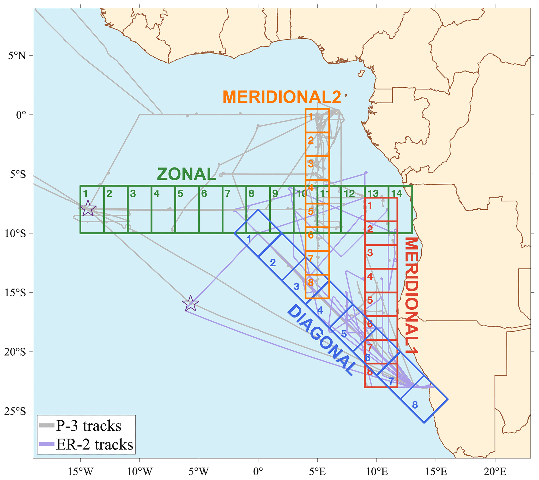
Figure 1 The four transects used in the model–observation comparison are shown along with the P-3 (2016, 2017, and 2018) and ER-2 (2016) aircraft flight tracks. Grid boxes within each transect are numbered from north–west to south–east. See Table S1 in the Supplement for the grid box coordinates. The locations of Ascension Island (8^∘ S, 14^∘ W) and St. Helena island (16^∘ S, 6^∘ W) are indicated with stars.

Figure 2 The number of minutes the P-3 aircraft spent in each grid box and 500 m altitude bin for the comparison transects shown in Fig. 1. The 2016 diagonal and 2017 and 2018 meridional 2 transects cover the routine flight tracks, which targeted semi-random sampling. Not all in situ measurements have data available for all times, so the number of minutes of available data may be less than the number of minutes the P-3 was present in a given grid box and altitude bin.

The large uncertainty in aerosol climate forcing in the SE Atlantic was the impetus for the NASA ORACLES (ObseRvations of Aerosols above CLouds and their intEractionS) project, funded through the NASA Earth Venture Suborbital (EVS-2) program (Redemann et al., 2021), as well as complementary campaigns (Zuidema et al., 2016; Formenti et al., 2019; Haywood et al., 2021). The ORACLES project explicitly measured aerosol properties necessary to calculate the direct aerosol radiative effect (DARE). The campaign included deployments of the NASA P-3 research aircraft to the SE Atlantic region based out of Walvis Bay, Namibia (27 August–27 September 2016), and São Tomé, São Tomé and Príncipe (9 August–2 September 2017 and 24 September–25 October 2018). The NASA ER-2 aircraft also deployed to Walvis Bay on 26 August–29 September 2016. The P-3 carried a suite of instruments to measure in situ gas concentrations and aerosol microphysical, optical, and chemical properties, to measure cloud microphysical properties, and to remotely sense both aerosols and clouds. It generally flew between 100 m and 6 km above the sea surface, capturing in situ data in ramped or spiral profiles, horizontal variations in level legs, and aerosol and trace gas columnar properties (e.g., aerosol optical depth – AOD) when flying below aerosol layers. The ER-2 flew at a high altitude (19 km) and carried remote sensing instruments only, observing both aerosols and clouds (see Redemann et al., 2021, for a more complete overview of the ORACLES campaigns).

Here, aerosol and cloud properties observed during the three ORACLES deployment periods are compared to two regional models, namely the Weather Research and Forecasting model coupled with the physics package of Community Atmosphere Model (WRF-CAM5) and the Centre National de Recherches Aire Limitée Adaptation dynamique Développement InterNational model (CNRM-ALADIN; hereafter simply ALADIN), and two global models, namely the Goddard Earth Observing System model (GEOS) and the United Kingdom Chemistry and Aerosols Unified Model (UM-UKCA). Descriptions of each model are given below. The WRF-CAM5 and GEOS models are included because they were used for aerosol and meteorological forecasting during the ORACLES campaign. Similarly, the UM-UKCA modeling team participated in the UK CLARIFY (Cloud–Aerosol–Radiation Interactions and Forcing) campaign, which deployed out of Ascension Island (Fig. 1) in 2017 (Haywood et al., 2021). In 2016, both ORACLES and the French AEROCLO-SA (AERosol, radiatiOn, and CLOuds in Southern Africa; Formenti et al., 2019) campaign deployed out of Walvis Bay, Namibia, with the latter focusing on near-coast aerosols. The ALADIN regional model version 6 used here (Mallet al., 2019, 2020; Nabat et al., 2020) simulated aerosol and clouds over the SE Atlantic as part of the AEROCLO-SA campaign.

The properties included here (Sect. 2.1) allow for a first-order calculation of DARE (Sect. 5). Forcing through aerosol–cloud interactions is driven by a more complex set of processes, including the time history of aerosols and clouds (Diamond et al., 2018), aerosol physical and chemical properties (e.g., McFiggans et al., 2006; Kacarab et al., 2020), the micro- and macro-physical properties of the clouds (e.g., Stevens and Feingold, 2009; Koren et al., 2014; Gupta et al., 2021), and the thermodynamic state of the atmosphere. There is limited treatment herein of this broader set of variables, though testing model accuracy in representing cloud fraction does provide a critical zero-order step toward determining whether models might be capturing processes key to quantifying forcing through aerosol–cloud interactions.

This study builds on the work of Shinozuka et al. (2020), which compared modeled and observed column aerosol properties for the September 2016 ORACLES deployment only. There, comparisons were presented as box-and-whisker plots of two-dimensional (2D; i.e., column) and three-dimensional (3D) variables. For 3D variables, values were binned into three discrete layers, i.e., the marine boundary layer, the free troposphere below 3 km, and 3–6 km altitude. The Shinozuka et al. (2020) study focused on comparisons of layer-averaged carbon monoxide (CO) and aerosol properties, as well as the smoke layer bottom and top altitudes. Comparisons were made to six models; in addition to the four included herein, the EAM-E3SM and GEOS-Chem models provided statistics for the variables analyzed in Shinozuka et al. (2020).

2 Comparison overview

The comparisons presented here focus on vertically resolved aerosol properties, where data are averaged into 500 m altitude bins from the surface up to 6 km and on the clouds below the biomass burning smoke plume. The observed and modeled aerosol and cloud properties are compared for multiple transects across the SE Atlantic (Fig. 1). Observed values of the aerosol properties are from the ORACLES research flights, while observed cloud properties are from satellite retrievals, since the calculation of cloud fraction and optical depth from observations made from the aircraft are too limited to be of use in the statistical comparison presented here.

2.1 Comparison variables

The focus is on variables that are strongly related to the direct aerosol radiative effect of biomass burning aerosol. Vertically resolved comparisons are made to variables measured in situ from the NASA P-3 and measured with the NASA High Spectral Resolution Lidar, HSRL-2 (σ_ep only), which deployed on the ER-2 in 2016 and the P-3 in 2017 and 2018. The compared variables are as follows:

• carbon monoxide (CO) mixing ratio

• black carbon (BC) concentration

• organic aerosol (OA) concentration

• light extinction (σ_ep; 530 nm from the in situ observations; 532 nm from the HSRL-2; 550 nm from the models)

• single scatter albedo (SSA; 530 nm from the observations; 550 nm from the models)

• aerosol absorption Ångström exponent (AAE; 440–670 nm for the observations; 400–600 nm for the WRF-CAM5, GEOS, and ALADIN models; 380–550 nm for UM-UKCA)

• aerosol scattering Ångström exponent (SAE; 440–670 nm for the observations; 400–600 nm for the WRF-CAM5, GEOS, and ALADIN models; 380–550 nm for UM-UKCA)

• relative humidity (RH).

The aerosol optical properties σ_ep, SSA, AAE, and SAE are measured in situ at low RH. The values of σ_ep retrieved from HSRL-2 and simulated by all four models are reported at ambient RH; the UM-UKCA model additionally reports dry σ_ep.

The properties most critical to the underlying cloud albedo – the cloud fraction and cloud optical thickness – are evaluated by comparing the following 2D cloud variables:

• mean warm cloud fraction (CF_warm)

• geometric mean warm cloud optical thickness (COT_warm).

These properties from the models are compared with those retrieved from the polar-orbiting Moderate Resolution Imaging Spectroradiometer (MODIS; CF_warm and COT_warm) and geostationary Spinning Enhanced Visible and InfraRed Imager (SEVIRI; CF_warm only).

2.2 Comparison transects, altitude bins, and statistics

Comparisons are made along several transects of grid boxes (Fig. 1; Table S1 in the Supplement). The locations of the transects are dictated by frequent research flight paths, which varied across the 3 years of the project. A decided focus of the ORACLES field campaigns was to devote about half of the P-3 flight hours in each year to sampling along routine flight tracks (Redemann et al., 2021). The explicit goal was to sample the transect across a set of randomly distributed days throughout the field deployment in order to build a dataset representative of the deployment month.

During ORACLES 2016, the routine flights followed a diagonal latitude/longitude transect (diagonal transect, shown in Fig. 1, terminating near Namibia). With deployment based out of São Tomé in 2017 and 2018, the routine flights were along a north–south-oriented track centered on 5E (meridional 2; see Fig. 1). The routine flight pattern usually consisted of a series of in-transit profiles and horizontal legs in the aerosol layer and in the boundary layer clouds. In 2017 and 2018, with the HSRL-2 lidar on board the P-3, the south-bound leg on routine flights was usually flown at an aircraft maximum altitude (approximately 5–6 km) to survey the aerosol and cloud layers below. The north-bound run was then a combination of vertical profiling, horizontal legs, and sawtooth legs (for clouds). Each routine flight included a different combination of legs and profiles, so only the latitude/longitude line of the flights (not their altitudes) were common to all. In 2016, on most routine flight days, the NASA ER-2 would also fly along the routine track and, in some cases, overfly the P-3.

In addition to the dedicated routine track in 2016, a significant number of P-3 target of opportunity flights (Redemann et al., 2021) were flown along a north–south transect near the southern African coast. As such, the meridional 1 (Fig. 1) set of comparison grid boxes is also selected. Finally, for all 3 years a zonal transect is established, running from Ascension Island to the west African coast. The zonal transect is located approximately at the latitudinal center of the southern African biomass burning plume, along the northern edge of the main stratocumulus deck. Free troposphere transport in this region is driven by the southern African easterly jet, which is centered around 8^∘ S (Adebiyi and Zuidema, 2016); as such, in the free troposphere, the zonal transect, to first order, covers a gradient in age from east (younger) to west (more aged).

The zonal transect is located significantly farther from the deployment bases than the other comparison transects, so most grid boxes in this transect have little P-3 data. In 2016, only the ER-2 had sufficient sampling for meaningful comparisons with models along this transect. In 2017, when the P-3 did a suitcase flight to Ascension Island (Redemann et al., 2021), there was some coverage of the westernmost zonal grid boxes. For the zonal transect, the only aerosol observations included in the comparison are profiles of σ_ep from the HSRL-2 on board the ER-2 in 2016. In all 3 years, comparisons of CF_warm and COT_warm are included along the zonal transect, since these observations are from satellites and thus have good statistics in all 3 years.

In the discussions below, grid boxes are numbered from northwest to southeast for the diagonal transect, north to south for the two meridional transects, and west to east for the zonal transect (Fig. 1). Averages within each deployment year cover the following dates:

• 30 August through 27 September 2016,

• 9 August through 2 September 2017, and

• 24 September through 25 October 2018.

These include the transit flights from Namibia (2016) and to and from São Tomé (2017 and 2018). For ease of reference, we refer to these as the September 2016, August 2017, and October 2018 monthly averages.

Observed and modeled statistics are calculated for 500 m deep altitude bins from the surface to 6 km, with two exceptions. Relative humidity is aggregated into 250 m deep bins to more clearly show the transition from the boundary layer to the free troposphere. Light extinction from the HSRL-2 has a 315 m vertical resolution, and this resolution is retained. Mean biases are calculated as the averages of the ratios in 1 km altitude bins for more robust statistics. For the in situ observations, data are included in statistics whether made on level legs or during profiles, so the number of data points included in statistics can vary significantly with altitude within a given grid box (Fig. 2).

The aerosol properties compared here were measured from the aircraft, and so are available on specific days and for specific locations on each flight. In the aerosol comparisons, the model statistics used are calculated for only those dates and locations where the aircraft was present. In contrast, the observed CF_warm and COT_warm statistics are from satellite-based measurements (Sect. 3.2) and thus are available for every day of each year's deployment. In this case, both observed and model statistics are calculated for every day of the deployment period across every comparison grid box.

To test for the representativeness of the observed aerosol properties, for some variables two sets of modeled statistics are calculated for each grid box and altitude layer, i.e., first for only those locations and times when the aircraft was present and second for all daylight hours (defined here as 06:00–18:00 UTC – universal coordinated time) across the duration of that year's deployment. Comparison of the two allows for testing the representativeness of the observations for assessing monthly averages, assuming that the model realistically captures aerosol variability. To test this, we calculated the fractional variability in σ_ep in the 2–5 km altitude range within the comparison grid boxes in the WRF-CAM5 and GEOS models and in the observations. We found that the three are similar for the 2016 diagonal and meridional 1 transect grid boxes, with the models alternately having lower and higher fractional variability than was observed. Along the 2017 meridional 2 transect, WRF-CAM5 and the observed variability were similar, but the GEOS variability was 10 %–30 % higher. Along the 2018 meridional 2 transect, the converse was true; the relative variability in σ_ep was similar for GEOS and the observations but was about 20 % lower for WRF-CAM5.

Shinozuka et al. (2020) also tested the representativeness of observed column properties (aerosol optical depth) for the September 2016 campaign only. The vertically resolved data provide additional, more detailed information on representativeness, which is something columnar passive satellite observations cannot provide. In addition, here representativeness is tested for all 3 campaign years.

3 Dataset descriptions

3.1 Observed aerosol properties, CO concentrations, and relative humidity

Detailed descriptions of the instruments used to measure aerosols and gases are given in Appendix 9.1 of Shinozuka et al. (2020). Here, the characteristics of each measurement most relevant to the presented comparison are discussed. All in situ observations are derived from the 1 s resolution data collected on the P-3, which are available from the NASA public data archive (see the Data Availability at the end of the paper). Several of the measurements used here (e.g., absorption; see below) are very noisy at this resolution. To reduce noise, the 1 s resolution data are smoothed using a weighted average, calculated with a Gaussian weighting function covering ±30 s on either side of each 1 s resolution data point. The weighting function has 61 values, with the peak at value 31. The standard deviation was set to 12; this produces a weighting function such that the data points at time t−30 and t+30 s are weighted at 4.4 % of the value at time t. A much larger standard deviation would have weighted values more than 30 s from the time of interest too heavily (e.g., by 17 % for a value of 16), and a much smaller standard deviation would have produced a weighting function that approached zero in less than 30 s. Values of in situ σ_ep, SSA, SAE, and AAE are derived after this smoothing function is applied to the scattering and absorption data. In all cases, statistics for a given altitude bin and comparison grid box are included for the in situ observations only if at least 10 min of data in total are available.

Aerosol optical properties were measured in situ at low (<40 %) RH via an aerosol inlet with a 50 % cutoff diameter of approximately 5 µm (McNaughton et al., 2007). Above the boundary layer, the aerosol during ORACLES was dominated by accumulation mode biomass burning smoke, with a volumetric mean diameter of <0.4 µm (e.g., see Fig. 8 of Shinozuka et al., 2020), so it is expected that the in situ instruments capture the properties of the vast majority of aerosol contributing to column radiative impacts and all of the biomass aerosol.

Carbon monoxide was measured with an ABB (Los Gatos Research) $\mathrm{CO}/{\mathrm{CO}}_{\mathrm{2}}/{\mathrm{H}}_{\mathrm{2}}\mathrm{O}$ analyzer modified for flight operations, with a precision of 0.5 ppbv (parts per billion by volume) for 10 s averages (Liu et al., 2017; Provencal et al., 2005). Black carbon was measured as refractory BC (rBC) using a single particle soot photometer (SP2; Schwarz et al., 2006; Stephens et al., 2003) calibrated with Fullerene soot. The SP2 measurement of rBC mass is estimated to have an uncertainty of 25 % at the provided 1 s resolution. A high-resolution time-of-flight aerosol mass spectrometer (HR-ToF-AMS; Aerodyne Research Inc.), operated in high-sensitivity V mode, was used to measure organic aerosol (OA) mass with an estimated accuracy of 50 % at 1 s time resolution.

Aerosol light scattering (σ_sp) at 450, 550, and 700 nm was measured on board the P-3 at low (<40 %) RH with a TSI (model 3563) nephelometer, with the corrections of Anderson and Ogren (1998) applied. In 2018, two TSI nephelometers were operated, with one periodically measuring the submicron aerosol only. When both were measuring the total aerosol, reported σ_sp is the average of the two. In 2018, the 450 nm channel on the nephelometer was not working, so SAE data are not available for that year.

As discussed below, most models report aerosol optical properties at ambient RH. Relative humidity profiles and aerosol hygroscopic growth factors inform whether this could be a significant source of differences between the modeled and observed aerosol optical properties and so are shown here. The observed ambient RH was calculated based on dew point measured using an Edgetech 137 Vigilant hygrometer. Hygroscopic growth factors for 530 nm light scattering were quantified during ORACLES, using a pair of Radiance Research nephelometers, run at low (<40 %) RH and approximately 85 % RH, respectively. However, there were instrumental issues that resulted in significant data gaps in 2016 and 2018 and instrumental problems across the full 2017 campaign. This complicates correcting to humidified scattering values for the statistical comparisons with the models. As such, here we use these data only to estimate the effect of humidification on scattering, based on aerosol characteristics aggregated across all observations (not just those in the comparison transects) within each field season.

Dry aerosol light absorption (σ_ap) at 470, 530, and 660 nm was calculated using measurements from one (2017 and 2018) or two (2016) three-wavelength Radiance Research particle soot absorption photometers (PSAPs). For 2016, the values from the two PSAPs are averaged; for 2017 and 2018 only one of the PSAPs consistently measured the total ambient aerosol absorption, so only data from that PSAP was used. Filter-based absorption measurements, such as the PSAP, are known to have loading-based artifacts that produce a positive bias that requires correction (e.g., Bond et al., 1999; Virkkula, 2010). Early versions of the PSAP instrument measured σ_ap at only one wavelength (530 nm), so correction factors at this wavelength are better understood than at 470 and 660 nm, where they are untested for accuracy. Here, two sets of correction factors have been applied to the PSAP dat, namely the wavelength-averaged and the wavelength-specific corrections, which are both described in Virkkula (2010). These correction factors are very similar at 530 nm but yield different values of σ_ap at 470 and 660 nm. They, therefore, yield different values of derived absorption Ångström exponent but nearly identical 530 nm SSA.

Scattering at the 450, 550, and 700 nm wavelengths (λ) is used to calculate a linear fit to log(σ_sp) versus log(λ), yielding the scattering Ångström exponent (SAE). The absorption Ångström exponent (AAE) is analogously calculated from σ_ap at 470, 530, and 660 nm for, as noted above, σ_ap derived using the two sets of Virkkula (2010) correction factors. The observed values of σ_ep and SSA included here are at 530 nm for low RH aerosol. They are calculated by adjusting the measured low RH 550 nm σ_sp with the above-calculated SAE. This adjusted σ_sp is then summed with the 530 nm σ_ap to obtain σ_ep, and SSA is calculated as the ratio of 530 nm σ_sp to 530 nm σ_ep. SAE and SSA are calculated only when σ_ep is greater than 10 Mm⁻¹, and AAE is only calculated when σ_ap is greater than 5 Mm⁻¹ in order to avoid including data dominated by noise.

All of the above measurements were made from the P-3 aircraft. Data from the airborne second-generation High Spectral Resolution Lidar version 2 (HSRL-2) that was flown on the ER-2 aircraft in 2016 and the P-3 in 2017 and 2018 are also included in the comparison. The HSRL-2 is a remote sensing instrument, so retrieved values of σ_ep are at ambient RH and, therefore, are more directly comparable to the modeled values. The HSRL-2 independently detects backscatter from aerosols and molecules using the spectral distribution of the returned signal, thereby retrieving σ_ep without having to make assumptions about the backscatter-to-extinction ratio of the aerosol (Shipley et al., 1983; Hair et al., 2008; Burton et al., 2018). The HSRL-2 retrieves σ_ep at 355 and 532 nm with 315 m vertical resolution; here, we use the 532 nm data only for comparison to modeled 550 nm σ_ep.

3.2 Observed cloud properties

From the standpoint of aerosol forcing, the clouds of most interest in the SE Atlantic are stratocumulus and cumulus (warm and low) clouds in the boundary layer, as these clouds are most prevalent in the region and underlie the aerosol plume, so they are a strong controlling factor on the direct aerosol radiative effect sign and magnitude. As such, here we compare the warm, low cloud (< 2.5 km, T>273 K) fraction (CF_warm) from models to that retrieved in several satellite products.

Cloud optical thickness for these clouds (COT_warm) is approximately log-normally distributed (e.g., Fig. S1 in the Supplement), so for COT_warm we compare the geometric mean of all values within the comparison grid boxes. This statistic was selected as being the most physically meaningful, since it more closely represents the cloud optical thickness and, therefore, cloud impact on scene albedo for heterogeneous scenes.

CF_warm and COT_warm are derived for several retrieval products and are compared to each other and to the observations. As described later (Sect. 4.4), the SEVIRI-LaRC (Langley Research Center) values of CF_warm (Sect. 3.2.3) and the MODIS-ACAERO (above-cloud aerosol) values of COT_warm (Sect. 3.2.2) are used as the benchmark for the comparison to the modeled values.

3.2.1 MODIS standard cloud products

The Collection 6 MODIS Level 3 (L3) daily cloud products (Platnick et al., 2015a) from both the Aqua (MYD08) and Terra (MOD08) satellites are used to calculate average warm cloud fractions (CF_warm). These L3 products are statistical aggregations at 1^∘ × 1^∘ resolution (latitude × longitude) of the MODIS Level 2 (L2) pixel-level cloud retrievals (Platnick et al., 2015b, 2017). Since Aqua and Terra are polar-orbiting satellites, their cloud retrieval statistics from the ORACLES comparison grid boxes are from, on average, 10:20 LT (local time; Terra) and 13:40 LT (Aqua). Herein we refer to these as the MODIS standard retrieved cloud properties.

The L3 MODIS variables used for CF_warm are Cloud_Retrieval_Fraction_Liquid and Cloud_Retrieval_Fraction_PCL_Liquid, with the latter allowing for inclusion of partly cloudy pixels. Data are excluded from statistics if the retrieved cloud top height is greater than 2.5 km in order to include only low warm clouds. These variables only include the Level 2 pixel population that is identified as liquid phase or overcast and that has successful cloud optical property retrievals, allowing classification as liquid clouds. As such, CF_warm may be smaller than the actual warm cloud fraction, depending on the rate of cloud optical property retrieval failure (see, e.g., Cho et al., 2015) and the prevalence of broken clouds and cloud edges in a retrieval pixel. For the selected comparison transects – and for this region in general – the fraction of mid-level and high clouds is low. For example, in 2016, warm, low clouds comprise, on average, 93 % or more of the clouds in the diagonal and meridional 1 transect grid boxes and the four easternmost zonal transect grid boxes. In the seven westernmost zonal grid boxes, > 99 % of the clouds are warm clouds. An exception is the grid boxes closer to the African coastline, where mid-level clouds, in particular, can be more frequent. This is consistent with the fact that most mid-level and high clouds in the region originate over the continent (Adebiyi et al., 2020), a phenomenon we observed directly during the field campaigns.

3.2.2 MODIS-ACAERO cloud products

Retrievals of cloud properties from satellite-imager-based observations can be affected by the presence of aerosol above the clouds, particularly when that aerosol is light-absorbing (Haywood et al., 2004; Coddington et al., 2010; Meyer et al., 2013). While retrieved CF is not significantly impacted, the retrieved COT will be. If not accounted for, the attenuation of cloud-reflected solar radiation due to aerosol absorption can be interpreted by satellite imager cloud retrieval algorithms as higher effective radii and as a lower COT. Therefore, in addition to the MODIS standard cloud retrievals, we calculate cloud statistics using the L2 (1 km resolution) MOD06/MYD06 ACAERO retrievals from MODIS that use the Meyer et al. (2015) approach, which accounts for the effects of the absorbing aerosol layer above low clouds and has been shown to produce COT values that compare better to aircraft-based observations than the MODIS standard product (Chang et al., 2021). These retrievals, referred to here as MODIS-ACAERO, simultaneously retrieve the above-cloud aerosol optical properties and the unbiased cloud optical properties and are used as the reference for observed COT_warm. (Specifically, the Cloud_Optical_Thickness_ModAbsAero parameter is used). The MODIS-ACAERO-retrieved CF_warm is also included, which differs from the MODIS standard definition in its use of cloud-top height (CTH) as an additional filter (specifically, CTH < 4 km; thus mid-level clouds are excluded). Otherwise, as with the MODIS standard retrievals, these are averages from the MODIS instruments on the Terra and Aqua satellites.

3.2.3 SEVIRI-LaRC cloud products

Warm clouds over the SE Atlantic have a significant diurnal cycle, particularly in cloud fraction (Rozendaal et al., 1995; Wood et al., 2002; Painemal et al., 2015). A question arises as to whether the MODIS retrievals, which make observations only twice daily, are representative of the daytime averages. The Spinning Enhanced Visible and Infrared Imager (SEVIRI) on the geostationary satellite Meteosat-10 views the SE Atlantic region at all times of the day. We use the cloud fraction retrieved from SEVIRI for three purposes. First, we calculate the average daytime CF_warm in each comparison grid box to test the modeled average daytime CF_warm. Second, we calculate the difference in the average daytime CF_warm and the average of CF_warm at 10:30 and 13:30 UTC only, as an estimate for how different CF_warm from the MODIS Terra and Aqua retrievals might be from an actually full daytime average of CF_warm. Third, as described below, we use the diurnal cycle in CF_warm to infer the diurnal cycle in COT_warm and, therefore, the representativeness of the MODIS-ACAERO Terra and Aqua COT_warm to the daytime average.

Here, the SEVIRI retrievals described by Minnis et al. (2008, 2011a, b) and Painemal et al. (2015) are used and are referred to as the SEVIRI NASA Langley Research Center (LaRC) retrievals. Warm cloud fractions are derived at 0.25^∘ grid resolution from pixel-level (3 km) retrievals by counting pixels with a liquid cloud phase and the effective cloud-top temperature T_cldtop> 273.2 K. Retrievals are provided every 30 min. We limit our analysis to daytime samples with solar zenith angles (SZAs) of less than 75^∘ to minimize retrieval uncertainties in the day–night transition.

In this region, cloud cover tends to be at a maximum in the early morning, then either decreases throughout the day or decreases until mid- to late afternoon, and then increases again (Fig. S2; Painemal et al., 2015). The average of CF_warm at 10:30 and 13:30 UTC is generally lower than, but within, 5 % of the daytime average (Table S2). The exception is at the northern end of the meridional 1 and meridional 2 transects, when the 10:30 and 13:30 UTC average is up to 14 % below the daytime average. While the 10:30 and 13:30 UTC average CF_warm is lower than the daytime average, it does represent CF_warm midday well, when solar flux (and, therefore, radiative forcing) is at a maximum.

An additional question is whether the COT_warm values from the 10:30 and 13:30 UTC MODIS-ACAERO retrievals are representative of the daytime average. The SEVIRI-LaRC retrievals do not simultaneously provide aerosol optical depth and cloud products, and inferred COT_warm could be biased if there is a high AOD layer above the clouds. To approximate the diurnal cycle in COT_warm, an empirical fit to COT_warm versus CF_warm from the MODIS-ACAERO dataset from all 3 field campaign years and comparison transects was used to approximate the difference between the 10:30 and 13:30 UTC average COT_warm and the average of COT_warm across the full daytime. The resulting fit (Fig. S3) is as follows:

$$\begin{array}{}\text{(1)}& {\mathrm{COT}}_{\mathrm{warm},\mathrm{fit}}=\mathrm{1.663}\times e^{\mathrm{1.982}\cdot {\mathrm{CF}}_{\mathrm{warm}}}.\end{array}$$

COT_warm, like CF_warm, is slightly lower – typically by less than 0.5 – for the 10:30 and 13:30 UTC average than for the full daytime average when calculated using the approximation in Eq. (1) (Table S3). At the northern end of the 2016 meridional 1 and 2017 meridional 2 transects, the difference is closer to 1.0. For a SZA of 30^∘, a decrease in COT_warm from 10.0, which is typical of clouds in this region (see Sect. 4.4), to 9.0 reduces cloud albedo by only 0.02, from 0.46 to 0.44 (see Sect. 5). The influence on scene albedo, which is the variable of interest for DARE, will be even smaller any time when CF_warm is less than 1.0. As such, the COT_warm values from MODIS appear to represent the daytime average, within the context of their role in determining aerosol direct radiative effects, very well.

3.3 Modeled aerosol and cloud fields

Data for all 3 ORACLES years are available for the WRF-CAM5 and GEOS models; UM-UKCA and ALADIN provided comparison data for the 2016 and 2017 ORACLES field campaign periods only. Statistics for all variables listed in Sect. 2.1 are provided for the WRF-CAM5 model. Statistics are not provided for RH from GEOS, for CO from UM-UKCA, or for CO, RH, and AAE for ALADIN.

All models report aerosol optical properties at ambient RH, in contrast to the observed optical properties which are at low RH. The UM-UKCA model also reports dry aerosol optical properties. In addition, all models report extinction and SSA at 550 nm, whereas the observed values are at 530 nm. Finally, the modeled AAE and SAE are calculated from 400 to 600 nm, whereas the observed AAE is calculated using σ_ap at the three wavelengths of 470, 530, and 660 nm and the SAE using σ_sp at 450, 550, and 700 nm.

The reported model CF_warm values are the mean of the grid box 2D warm, low cloud fractions, i.e., the fraction of the grid box covered by cloud as viewed from above, and not the fraction of the 3D grid box filled by cloud. Modeled CF_warm values exclude mid- and high-altitude clouds and include all low-lying warm clouds. This 2D CF is roughly equivalent to what would be observed via satellite and is the relevant quantity when interested in short-wave radiative forcing. For all models, 3D cloud fractions are converted to 2D warm, low cloud fractions (CF_warm) by assuming a maximum horizontal overlap in clouds at different altitudes within the same model column. As with the observed mean COT_warm values, the model mean COT_warm for each grid box is the geometric mean (Sect. 3.2), with one exception, namely for the ALADIN model, where the geometric mean COT_warm statistic was not calculated, so the median COT_warm is used instead.

Details on each model are given in Sect. 9.2 of Shinozuka et al. (2020), with brief descriptions given here. WRF-CAM5 is the regional Weather Research and Forecasting model with chemistry (WRF-Chem) coupled with the Community Atmosphere Model v.5 (CAM5) physics (Ma et al., 2014) with updated aerosol activation parameterizations (Zhang et al., 2015a, b). Here, the model is run at 36 km horizontal resolution and with 74 vertical layers varying in resolution from 10 to 500 m, with a higher resolution at lower altitudes. Aerosol mass and number are tracked, and aerosol optical properties are calculated with Mie code, assuming an internally mixed aerosol with three aerosol modes (Aitken, accumulation, and coarse). Cloud formation is driven by the shallow convection scheme of Bretherton and Park (2009) and deep convection by the Zhang and McFarlane (1995) scheme with interactive aerosols. Smoke emissions are initialized daily from the Quick Fire Emissions Dataset version 2 (QFED2; Darmenov and Da Silva, 2015), which provides emissions on a daily basis. Smoke is emitted directly into the boundary layer without using any plume injection parameterization. The model is initialized every 5 d using the National Centers for Environmental Prediction National Centers for Environmental Prediction Final Operational Global Analysis (NCEP FNL) and CAMS reanalysis and runs for 7 d, with the first 2 d of the run used for spin-up. Data are output at a 3 h time resolution and aggregated for statistics.

The GEOS (Goddard Earth Observing System v. 5) global model (Molod et al., 2015; Rienecker et al., 2008), often referenced as GEOS-FP (GEOS forward processing), is the forecast system of NASA's Global Modeling and Assimilation Office. It is run in near-real time at approx. 25 km horizontal resolution (0.25^∘ in latitude, 0.3125^∘ in longitude) and 72 vertical layers (of which 25 layers are between the surface and 400 hPa). The model is initialized every 12 h, with aerosol fields saved every 3 h and cloud fields hourly. The model is initialized using the Modern-Era Retrospective analysis for Research and Applications, version 2 (MERRA-2), reanalysis product, so it includes an assimilation of observed AOD data. This nudging towards observed AOD should improve this model's simulated σ_ep values relative to a free-running model. Like WRF-CAM5, GEOS also uses QFED2 biomass burning emissions and injects the emissions at the surface. It prognostically predicts CO, aerosol component masses, and ambient RH aerosol optical properties using GOCART (Goddard Chemistry Aerosol Radiation and Transport; Chin et al., 2002; Colarco et al., 2010). It assumes that aerosols are externally mixed in modes of fixed mean diameter and standard deviation. Optical properties are computed for each aerosol species included in GOCART and as a function of RH (Randles et al., 2017; Colarco et al., 2014). GEOS assimilates AOD observations from remote sensing every 3 h (Albayrak et al., 2013). Organic aerosol (OA) concentration is not provided explicitly by GEOS but organic carbon (OC) is. The ratio $\mathrm{OA}/\mathrm{OC}$ =1.4 is used to obtain the reported OA concentrations. Both hydrophilic and hydrophobic BC and OC are simulated; the masses reported here are from the sum of the hydrophilic and hydrophobic components. Clouds are simulated by the convective parameterization.

The UM-UKCA is a global model that forecasts aerosols and clouds and is run here with a configuration modified from that used in Gordon et al. (2018), which also focused on the SE Atlantic. The model resolution varies with latitude (N216 resolution), with approximately 60 km ×90 km resolution at the Equator. It has 70 vertical levels between the surface and 80 km altitude, with a decreasing vertical resolution such that the grid spacing at 1.5 km altitude is approximately 200 m. It is nudged to horizontal wind fields (not to temperature) from ERA-Interim reanalyses, with nudging starting at 1700 m above the surface and ramping up to its full strength at 2150 m altitude. The reanalysis files are read every 6 h, which is also the relaxation time for the nudging. The model is run continuously forward from the initialization used by Gordon et al. (2018). In contrast to WRF-CAM5 and GEOS, biomass burning emissions are updated daily using the FEER (Fire Energetics and Emissions Research) inventory (Ichoku and Ellison, 2014). Smoke aerosol is emitted into and distributed through the boundary layer, such that concentrations are highest at the surface and then taper down to zero at 3 km above the surface (Gordon et al., 2018). The emitted smoke has an initial log-normal size distribution, with a mode centered on 120 nm diameter. Sea salt emissions are based on winds, no dust emissions are included, and all other emissions are from the CMIP5 inventories. Aerosols in the model are represented in five sized modes of internally mixed aerosol. Both dry and ambient RH aerosol properties are tracked, with hygroscopicity based on Petters and Kreidenweis (2007). Convection is represented using the pc2 subgrid cloud scheme of Wilson et al. (2008) or is parameterized where it cannot be resolved.

The ALADIN model is a regional climate model developed at Météo-France/Centre National de Recherches Météorologiques (CNRM). The version (v.6) used here has a more detailed treatment specifically of biomass burning aerosols than previous versions (Mallet et al., 2019, 2020). The model has 12 km horizontal resolution and 91 vertical levels, with 28 located between the surface and 6 km altitude. Lateral boundary conditions and the initial state for the modeled region come from the ERA-Interim reanalysis (Dee et al., 2011). The model includes TACTIC (Tropospheric Aerosols for Climate In CNRM; Nabat et al., 2020) which includes sea salt, desert dust, sulfates, and black and organic carbon separated in 12 aerosol size bins. All emissions come from the CMIP6 emissions inventory (van Marle et al., 2017), which uses the Global Fire Emissions Database (GFED) for biomass burning emissions. This inventory has realistic biomass burning emissions only through 2014, so these runs were done using constant year 2014 emissions. Furthermore, while the BC emissions from GFED are used, ALADIN uses a fixed particulate organic matter (POM) to organic carbon (OC) ratio, based on Formenti et al. (2003), so secondary organic aerosol formation is not accounted for. The radiative properties of liquid clouds are calculated in the short wave using the Slingo and Schrecker (1982) parameterizations. The atmospheric physics has recently been revisited, as described in detail in Roehrig et al. (2020). For the model runs used here, the first indirect effect was not simulated, and the cloud droplet effective radius was held fixed at 10 µm.

4 Results

The representativeness of the sampled aerosol properties to that of the entire field campaign period within each deployment year are discussed in Sect. 4.1. Biases in modeled extensive properties (CO, BC, and OA concentrations and σ_ep) are then discussed in Sect. 4.2, in aerosol intensive properties (SSA, SAE, and AAE) in Sect. 4.3, and in clouds (CF_warm and COT_warm) in Sect. 4.4.

4.1 Representativeness of observations

As discussed above, a goal of flying along the routine track was to acquire data representative of the observation period rather than, e.g., targeting high-concentration plumes. With limited flight hours and in situ sampling from the P-3 at specific altitudes on each flight track, the number of minutes spent in many of the grid boxes and altitude bins was of the order of 1–2 h in total over the approximately month-long campaign in each year; for some grid boxes and altitudes, it was <20 min (Fig. 2). The amount of data collected is particularly limited at the far reach of the comparison transects, i.e., the northwesternmost and northernmost grid boxes in the 2016 diagonal and meridional 1 transects and the southernmost grid boxes in the 2017 and 2018 meridional 2 transect. For the zonal transect, in situ sampling was extremely limited, with significant sampling only in 2017 in the westernmost zonal grid boxes 1 and 2 (from the suitcase flights to Ascension Island; Redemann et al., 2021) and in grid box 11, which intersects with the meridional 2 routine track.

Figures 3 and 4 show the ratios of the average of σ_ep in the model for those times when the aircraft was present for sampling (in situ for the P-3 and of the full column below the aircraft for the HSRL-2 on the ER-2 aircraft; i.e., sampled) to the daytime average for the full duration of the field deployment that year (climatology). Shinozuka et al. (2020) tested the representativeness of the observed column properties to the full month of the 2016 campaign period using as a metric the mean bias (MB) and the root mean squared deviation (RMSD) of CO and aerosol properties, along with their ratio (percent) to the monthly mean. They calculated MB and RMSD across grid boxes for data within broad altitude ranges, including the range of 3–6 km. Here we test for representativeness through the ratio of the means in 1 km deep altitude bins for each grid box (colored dots in Figs. 3 and 4). This metric is the same as MB(%) $/$ 100+1. This selection was made because the RMSD gives greater weight to individual large deviations, and the focus of this paper is on the average bias in observed values, which will most directly scale with a mean bias in DARE. In addition to calculating the mean bias for each grid box, the transect mean bias is calculated across all grid boxes in a given comparison transect and altitude bin (open circles in Figs. 3 and 4).

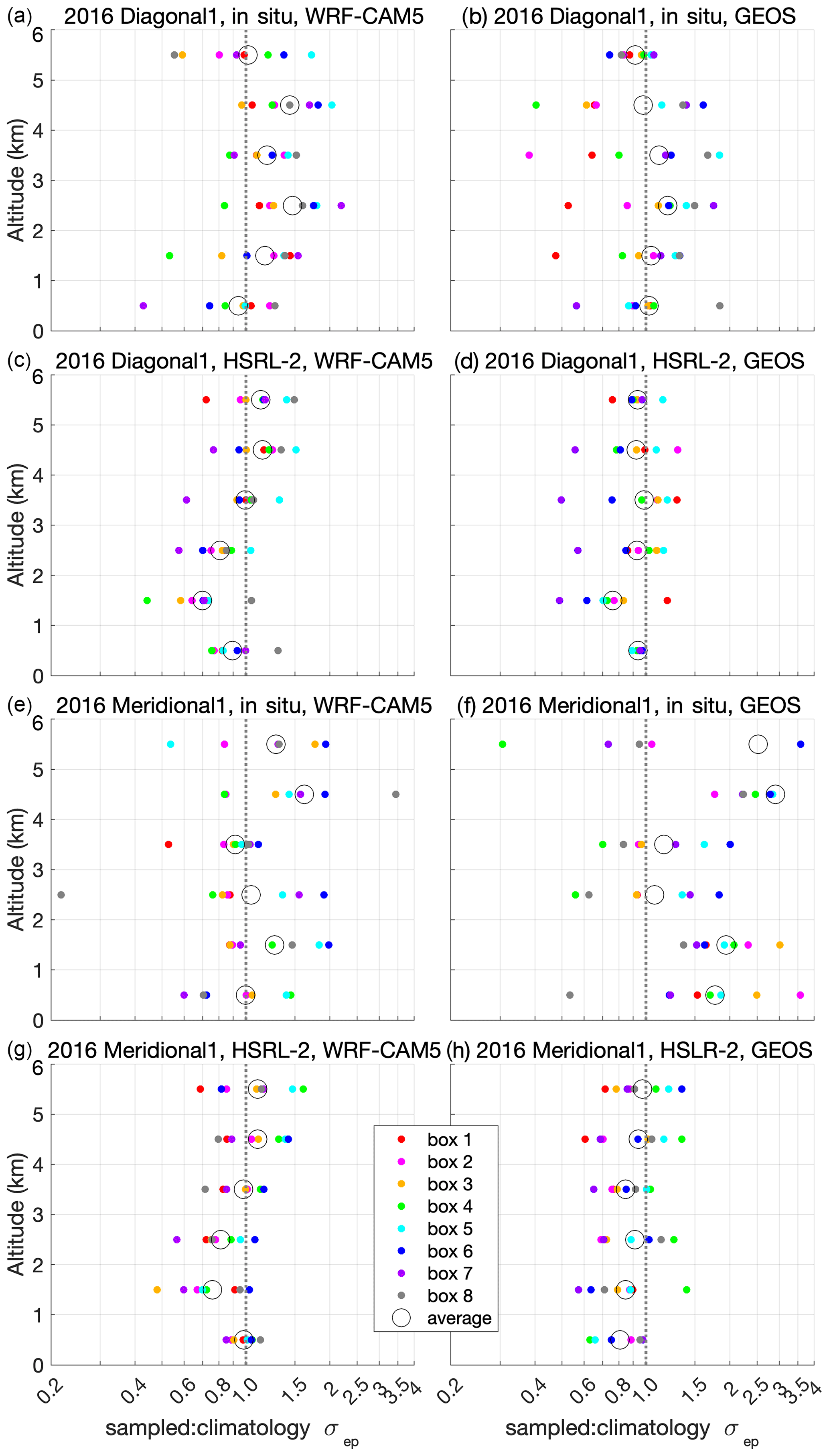
Figure 3 The ratio in the mean of σ_ep modeled by WRF-CAM5 (a, c, e, g) and GEOS (b, d, f, h) for only those times when observed values are available (sampled) to the mean of σ_ep across the entire field campaign time period (climatology) in the (a–d) diagonal transect in September 2016 and the (e–h) meridional 1 transect in September 2016. The representativeness of both the in situ (a, b, e, f) and HSRL-2 (c, d, g, h) observations of σ_ep are shown. The color dots show the means within individual comparison grid boxes; open circles are the mean across all grid boxes in that transect. Note that, in panel (f), there is a single grid box data point that is off scale (sampled : climatology σ_ep>4).

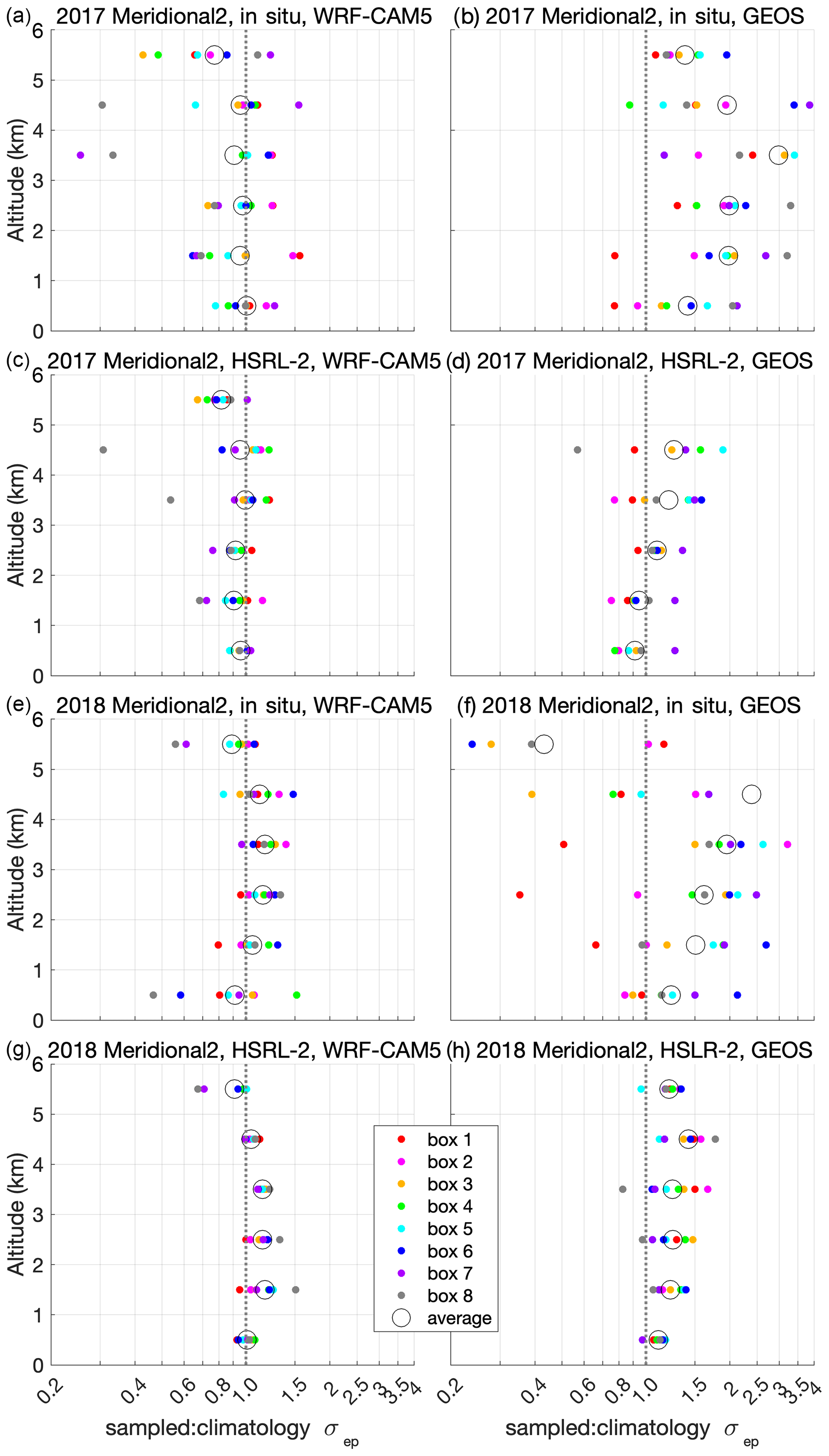
Figure 4 As in Fig. 3 but showing the representativeness of sampled σ_ep values to the month-long average of σ_ep across the 2017 meridional 2 and 2018 meridional 2 transects.

Both WRF-CAM5 and GEOS indicate that σ_ep at plume altitudes (2–5 km) along the 2016 diagonal transect is, on average, somewhat higher during the times sampled by the P-3 than it is for the monthly average (Fig. 3a, b), consistent with the findings of Shinozuka et al. (2020) in their AOD comparisons. The transect mean ratio is up to a factor of 1.5, depending on the altitude and model, with WRF-CAM5 showing larger and less variable differences than GEOS. Values of σ_ep at the times measured by the HSRL-2 from the ER-2 better represented the month-long average (Fig. 3c, d), with mostly moderate differences (ratios of 0.8–1.2) according to GEOS. In WRF-CAM5, the ratio of the sampled σ_ep to the month-long climatology increases with altitude from 2 to 6 km, indicating that the sampled plume may have been centered at higher altitudes than was typical for that month.

The 2016 meridional 1 transect is not a routine flight track, so sampling was on flights targeting the smoke plume and/or specific cloud fields and includes fewer observations than the diagonal transect (Fig. 2). As such, it was not expected to be as representative of the monthly average. Despite this, in the heart of the plume (2–4 km altitude), sampled values of σ_ep were generally within 0.9–1.2 of the month-long climatology in both models (Fig. 3e, f). Both models also indicate that smoke concentrations sampled by the P-3 at higher altitudes (4–6 km) are much higher than was typical. Values of σ_ep from times when the HSRL-2 could make observations from the ER-2 are more consistently representative of the month-long average, with transect mean ratios in most altitude bins above 2 km and between 0.8 and 1.2 (Fig. 3g, h). As for the 2016 diagonal transect, the WRF-CAM5 simulations indicate that the sampled plumes were centered at a higher altitude than is typical for this month.

The two models give very different results regarding the representativeness of both the in situ and HSRL-2 values of σ_ep to the month-long climatologies along the meridional 2 transect in both 2017 and 2018. The WRF-CAM5 model indicates that σ_ep in the 2–6 km altitude range for both in situ and HSRL-2 sampling was generally 0.8–1.2 times that of the month-long climatology and was almost always within a factor of 2 for individual grid boxes in the 2–5 km altitude range (Fig. 4a, c, e, g). GEOS simulations, however, show significantly higher values of σ_ep in the P-3 sampling average than in the month-long climatology for almost all grid boxes and altitudes. It also shows much greater variability across the different grid boxes in the sampling bias. As noted in Sect. 2.2, σ_ep in GEOS had a higher relative variability than observed along the 2017 meridional 2 transect, whereas WRF-CAM5 had similar variability to that observed and, therefore, may present a better test of the representativeness of the observations.

Overall, the values of HSRL-2 σ_ep sampled by the HSRL-2 are more representative of the climatology than the in situ values, likely because there simply were more samples gathered by the HSRL-2. Typically, the HSRL-2 retrievals are available in full curtains from just below the aircraft flight level to either the surface or cloud top from the southbound leg. In 2016, the HSRL-2 was on the ER-2, which always flew fully above the plume, so it captured the full vertical extent of the plume. In 2017 and 2018, when it was on board the P-3, the HSRL-2 generally could capture most of the plume vertical extent during the outbound leg of routine flights along the meridional 2 transect, since they were flown at high altitude. A combination of in situ measurements and HSRL-2 measurements would then be collected on the return, the northbound leg, which was flown at a variety of altitudes. As such, there are more data from the HSRL-2 than from the in situ measurements to contribute to comparison statistics.

In 2016, the ER-2 flew along the zonal transect on several flights (Fig. 1). WRF-CAM5 and GEOS both simulate average σ_ep from HSRL-2 sampling times that are, on average, within 0.8–1.2 of the month-long average in the 2–5 km altitude range (Fig. 5). This ratio is both more positive and more variable across grid boxes for 4–5 km than for 2–4 km or 5–6 km. This likely reflects the sampling coincidence with individual elevated plumes during the ER-2 flights.

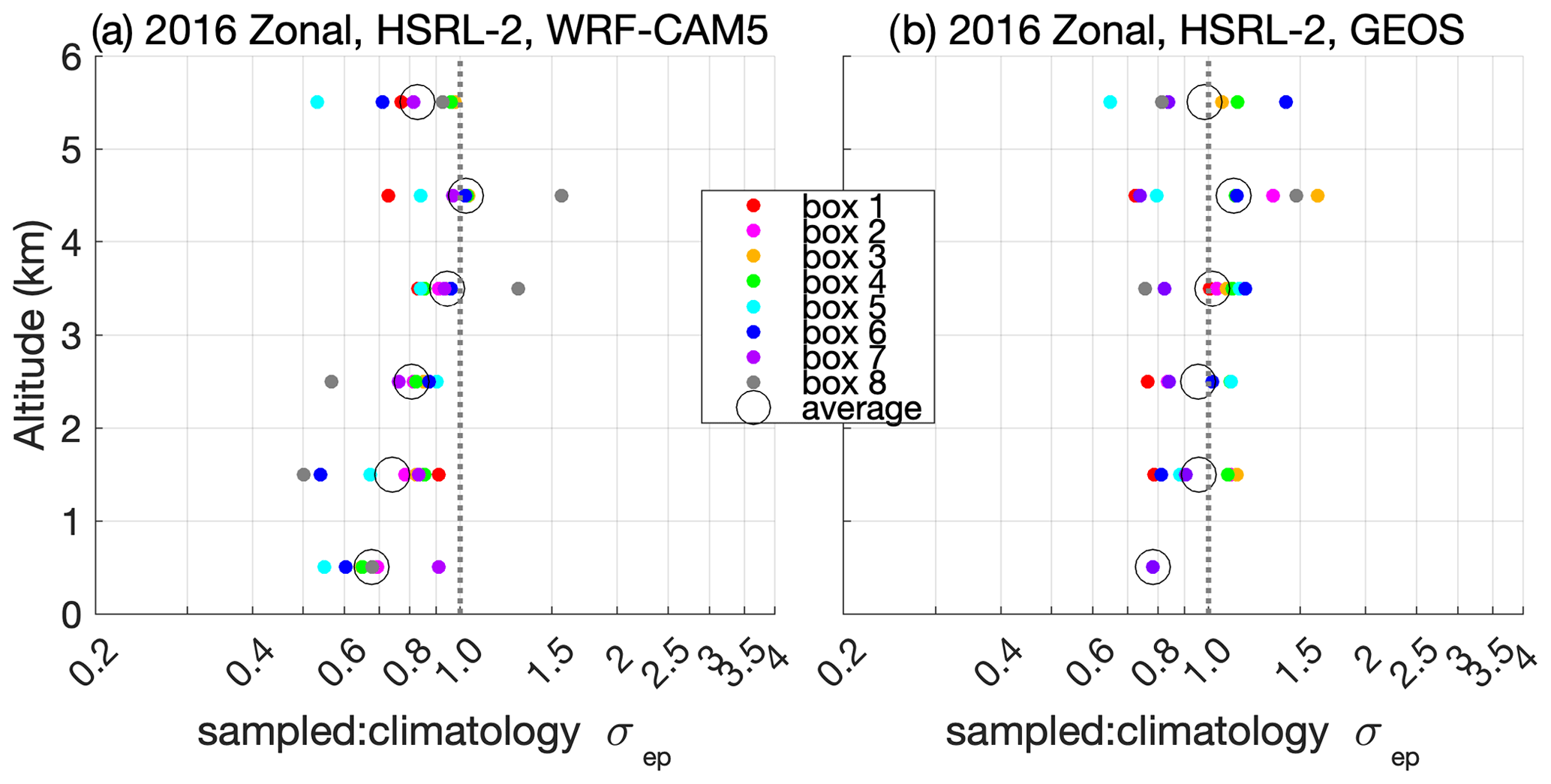
Figure 5 As in Fig. 3 but for the 2016 zonal transect and for the HSRL-2 retrievals of σ_ep only.

In 2017, σ_ep from both the in situ and HSRL-2 sampling times poorly represent the August average for most grid boxes and altitudes (Fig. S4), and in 2018 the P-3 did not fly along the zonal transect. For this reason, comparisons are not made of modeled and measured aerosols along the zonal transect. Clouds (CF_warm and COT_warm) were measured by satellite on all field campaign days, so comparisons of these fields along the zonal transect are included for all 3 years.

Tests of the representativeness of σ_ep measured from the aircraft addresses sampling biases in the concentration of the aerosol. In the context of DARE calculations, an additional question is whether the optical properties of the sampled aerosol are representative. Aerosol SSA in particular is a strong controlling factor for the sign and magnitude of DARE. In the WRF-CAM5 model, SSA of the aerosol in the 2–6 km altitude range at the times when there are in situ measurements from the P-3 are generally within 0.01 of the month-long average for that campaign year (not shown). SSA deviations from the average were a bit larger in the GEOS model in some grid boxes at these altitudes. In particular, in the meridional 2 transect, the aerosol measured in the two southernmost grid boxes in 2017 has an anomalously low SSA (by about 0.03–0.04), and in 2018, the SSA for 4–5 km is similarly anomalously high. These two grid boxes were the most undersampled in the meridional 2 transect, since they were the farthest from the deployment base. As will be seen below, the observed SSA varied more than the WRF-CAM5-modeled SSA, but less than the GEOS-modeled SSA, so the apparent representativeness of the sampled aerosol SSA may be a reflection of an inherent invariance in SSA in the models rather than an indication of the actual representativeness of the sampled aerosol optical properties.

4.2 Biases in plume extensive properties

Biomass burning smoke from the African continent is advected over the SE Atlantic largely in the free troposphere, and this is reflected in the observed profiles of σ_ep across the comparison transects (Figs. 6–9). This continental air mass carries water vapor with it (Pistone et al., 2021), though RH in the plume is still generally less than 60 % in September 2016 and August 2017 and less than 70 % in October 2018, except in the two northernmost grid boxes of the meridional 2 transect in 2018 (Figs. 10 and 11). The impact of humidification on σ_ep and on this comparison is discussed in Sect. 4.2.3.

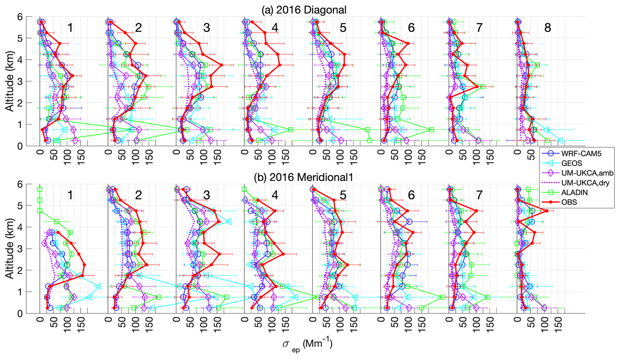
Figure 6 Profiles of σ_ep, as observed in situ from the P-3 aircraft (low RH; 530 nm), and modeled (ambient RH and, for UM-UKCA only, dry; 550 nm) for (a) the 2016 diagonal transect and (b) 2016 meridional 1 transect. All values are means and standard deviations calculated across only those times and locations when in situ measurements were made. Grid boxes are numbered as in Fig. 1.

Figure 7 As in Fig. 4 but for the (a) 2017 and (b) 2018 meridional 2 transect.

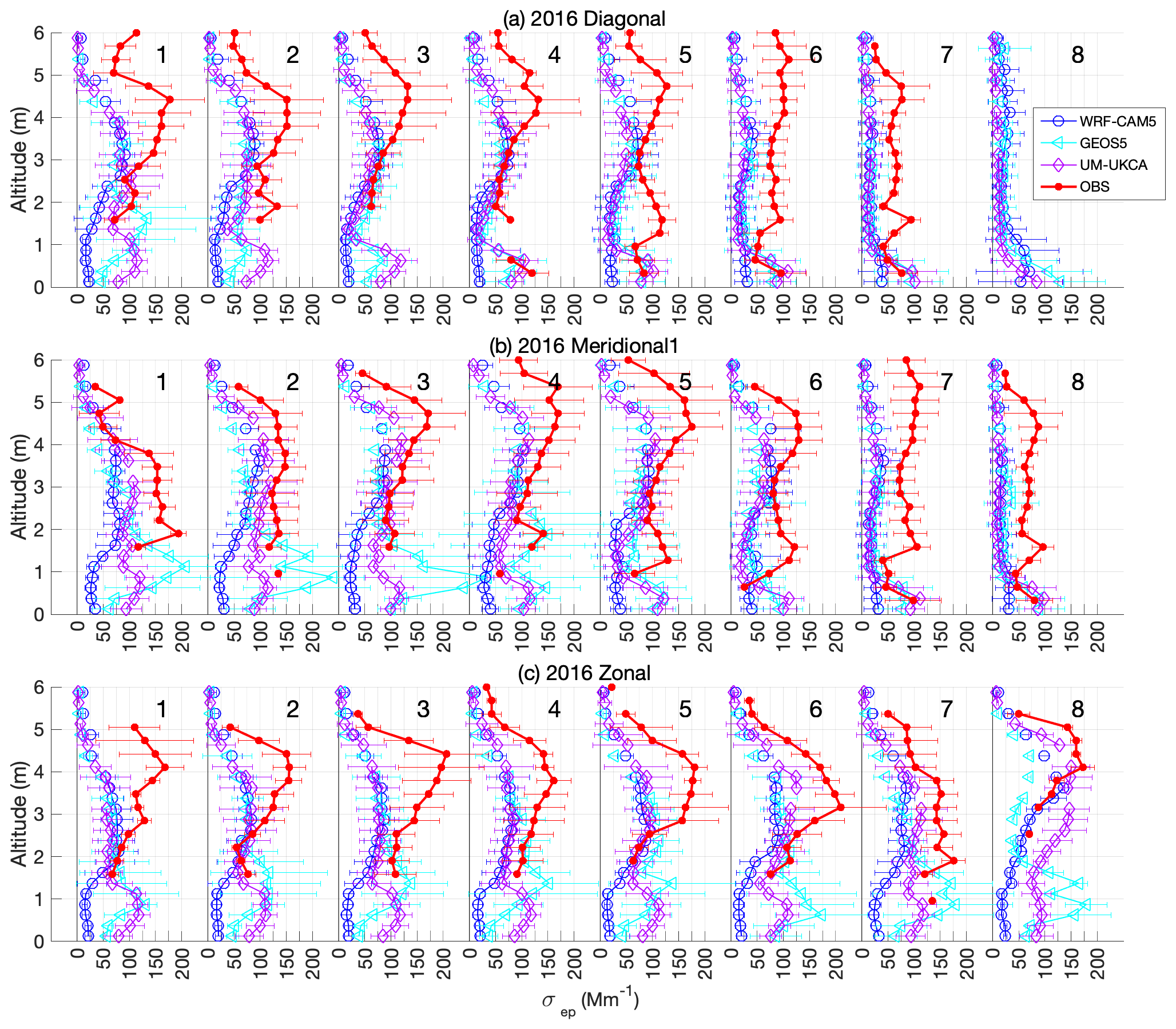
Figure 8 As in Fig. 6 but for the HSRL-2 retrievals of σ_ep from the ER2 aircraft in 2016. Here, all values are at ambient RH.

Figure 9 As in Fig. 8 but for the HSRL-2 retrievals of σ_ep from the P-3 aircraft along the (a) 2017 and (b) 2018 meridional 2 transect.

Figure 10 As in Fig. 6 but for RH and at 250 m vertical resolution rather than 500 m vertical resolution.

Figure 11 As in Fig. 10 but for RH along the (a) 2017 and (b) 2018 meridional 2 transect.

Analogous figures showing profiles of the other extensive variables can be found in the Supplement (see Figs. S5 for CO, S6 for BC, and S7 for OA). In the sections below, the modeled-to-observed ratios of these parameters are discussed; these should be viewed in the context of the smoke plume distribution (Figs. 6–9), since large biases in the core of the smoke plume have much greater impact than large biases where concentrations are low.

4.2.1 Carbon monoxide (CO)

Carbon monoxide does not lead to climate forcing, but it is an excellent and relatively inert tracer of biomass burning emissions and so is discussed here. WRF-CAM5-modeled CO at plume altitudes (2–5 km) is typically around 70 % to 80 % of that observed, with a slightly greater low bias in 2018 (Table 1 and Fig. S5). GEOS also has a low bias in CO at plume altitudes, but the biases are somewhat smaller and were more variable than for WRF-CAM5. In 2016 and 2017, the GEOS CO concentrations are increasingly biased low going from 2 km to 5 km altitude. In 2018, the GEOS biases are more consistent (0.6–0.8; Table 1) across almost all altitudes and grid boxes. The GEOS-modeled plume extends to lower altitudes than observed (Fig. S5), so that, for the 1–2 km altitude bin, the overall low bias in modeled CO is effectively offset by the contribution of the lower part of the modeled plume. Near the surface (0–1 km), CO in both WRF-CAM5 and GEOS is biased as low. CO was not reported for the UM-UKCA and ALADIN models. The biases in WRF-CAM5 and GEOS suggest underestimates in CO emissions, or possibly in the efficiency of transport of the biomass burning plume over the SE Atlantic from the burning source regions, since CO is not affected by scavenging processes. An earlier evaluation, by Das et al. (2017), of GEOS simulations of the SE Atlantic biomass burning plume compared to Cloud–Aerosol Lidar with Orthogonal Polarization (CALIOP) lidar profiles indicated that, for that model, transport biases are the more likely explanation.

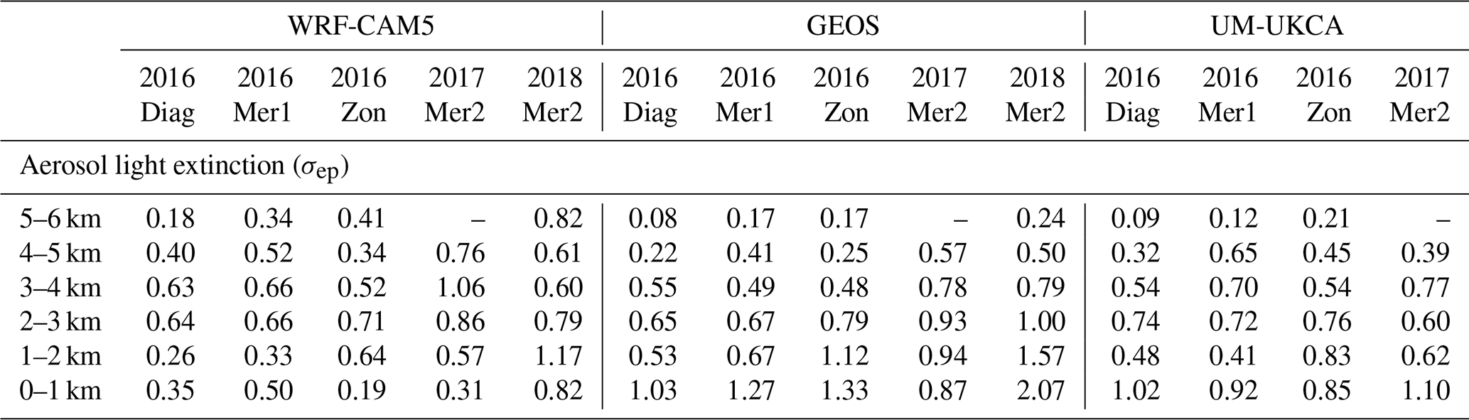
Table 1 Median across each comparison transect of modeled-to-observed ratios for extensive parameters averaged within 1 km deep altitude bins. Shown are median biases for CO concentrations, BC mass, OA mass, and σ_ep as measured in situ from the P-3 aircraft. Observed values of σ_ep are at 530 nm and for low RH (<40 %) aerosol, whereas modeled values are at 550 nm and ambient RH, except for UM-UKCA, which reports σ_ep for both the dry and ambient RH aerosol.

4.2.2 Aerosol BC and OA masses

During ORACLES, the aerosol components BC and OA were measured in situ and were reported for the WRF-CAM5, GEOS, and UM-UKCA models. In addition to emissions and transport processes, accurate simulation of aerosol concentrations requires simulating loss processes, including dry and wet deposition and any in-atmosphere production or loss. During the biomass burning season (July–October), south of ∼ 2–3^∘ S latitude in the SE Atlantic, there are few clouds with tops above 2 km, with small drop sizes further discouraging the wet scavenging of aerosols from the free troposphere (Adebiyi et al., 2020). For the 2016 diagonal comparison grid boxes, and for all but the northernmost two to three meridional 2 grid boxes in 2017 and 2018, almost all wet scavenging occurs in moist convection over the central African continent (Ryoo et al., 2021). Once over the ocean, wet deposition likely plays essentially no role in driving aerosol gradients in latitude and longitude above the marine boundary layer across our comparison transects, except possibly in meridional 2 grid boxes 1–3 (located between 0.5^∘ N and 5.5^∘ S). Fall speeds for accumulation-mode aerosols are, at most, a few meters per week; given that the biomass burning smoke is largely advected over the ocean at altitudes >2 km, dry scavenging rates will also be negligible. The vertical position of the plume and how it changes with transport is, therefore, dominated by the overall atmospheric convection and subsidence.

BC and OA are the primary constituents of biomass burning aerosol, so their distribution is a direct measure of the smoke plume intensity and location. On average, the observed core of the plume is centered at higher altitudes moving towards the edges of the plume (i.e., the southern end of the meridional 1 transect and the southeastern end of the diagonal transect in 2016 and the northern end of the meridional 2 transect in 2017 and 2018), and it covers a broader vertical extent towards the geographic center of the plume (Figs. 6–9, S6, and S7). In 2016 in particular, this tendency is not captured by any of the models, which have a vertically broader plume across all grid boxes and, in the case of GEOS and UM-UKCA especially, place the plume core at too low an altitude, though the plume top height is nonetheless captured properly in some cases (Shinozuka et al., 2020).

This overly vertical diffuse plume in WRF-CAM5 is consistent with underestimates in BC concentrations in the core of the plume (3–4 km altitude in 2016 and 2018; 3.5–5 km in 2017; Figs. 12 and 13), overestimates above this, and smaller biases for the 2–3 km altitude bin. The pattern of bias is similar for GEOS, except that it does a better job of reproducing BC concentrations aloft at the southern end of the 2016 meridional 1 transect (Fig. 12) and has greater high biases at the bottom of the plume (2–3 km altitude bin). UM-UKCA BC in the 2016 diagonal transect in the 3–5 km altitude range is about half that measured; in the 2016 meridional 1 and 2017 meridional 2 transects, biases in modeled BC are smaller (generally 0.70–0.85 at plume altitudes; Figs. 12 and 13; Table 1). In 2016, as with GEOS, the fact that the plume is too low in altitude results in large negative biases at the highest altitude, but there is a low bias below this that decreases from 5 to 2 km altitude. Both GEOS and UM-UKCA overestimate the amount of BC (i.e., biomass smoke) that mixes into the marine boundary layer, with consequences for derived forcing through aerosol–cloud interactions.

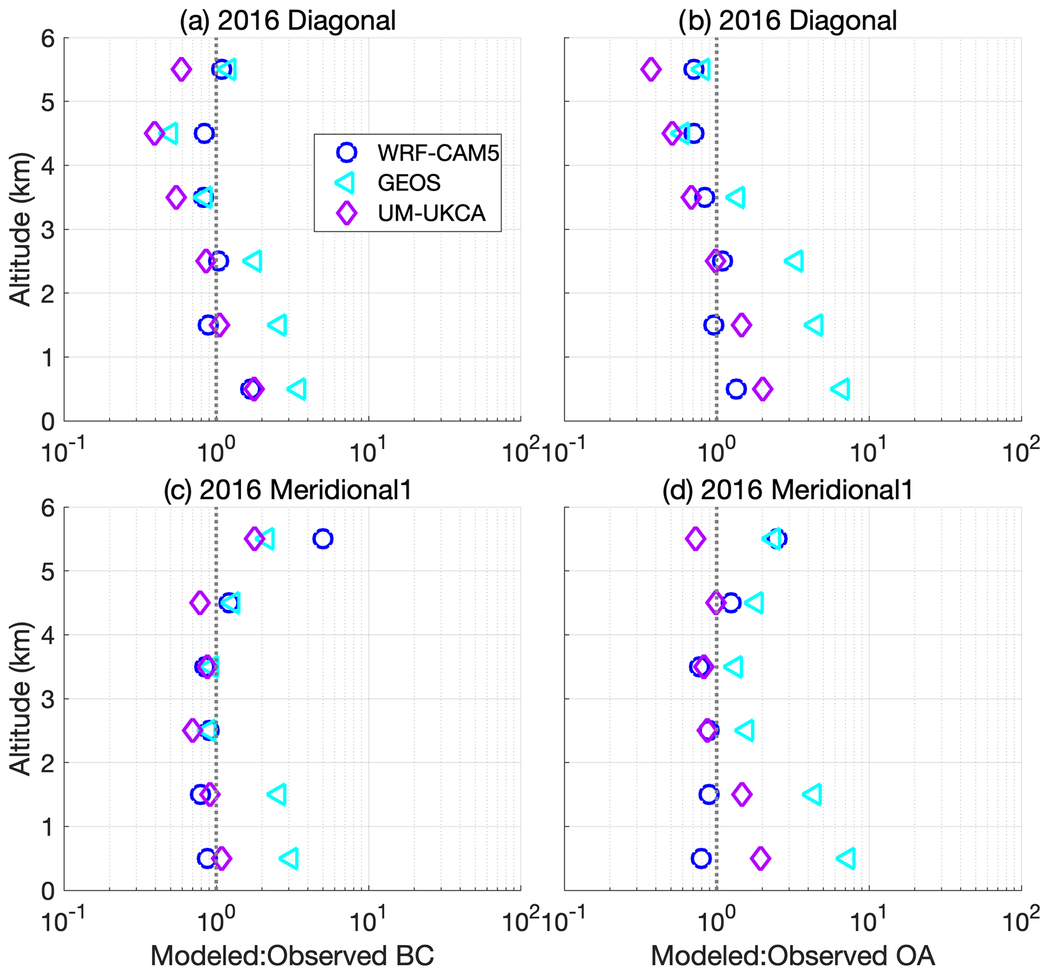
Figure 12 Mean ratio of modeled-to-observed BC mass (a, c) and OA mass (b, d) across all eight grid boxes along the 2016 diagonal (a, b) and meridional 1 (c, d) comparison transects. The ratios for individual grid boxes, along with these means, can be seen in the Supplement (Fig. S8 for WRF-CAM5, Fig. S10 for GEOS, and Fig. S12 for UM-UKCA).

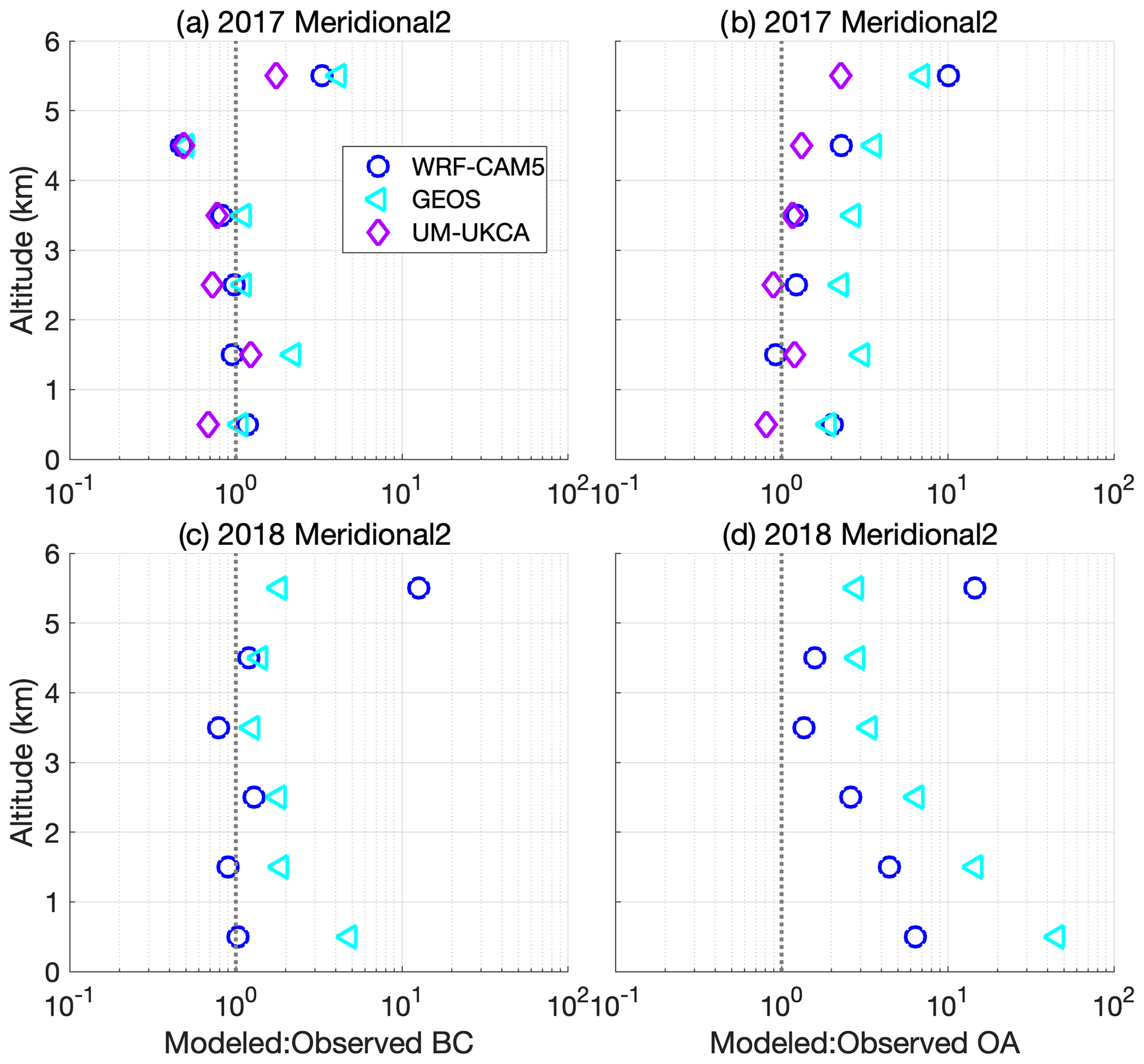
Figure 13 As in Fig. 12 but for the 2017 and 2018 meridional 2 comparison transect. The ratios for individual grid boxes, along with these means, are given in the Supplement (Fig. S9 for WRF-CAM5, Fig. S11 for GEOS, and Fig. S13 for UM-UKCA).

In several of the transects, above 5 km the observed BC and OA concentrations effectively go to zero (Figs. S6 and S7), whereas, for all models, the aerosol concentrations taper off more slowly, possibly due to coarse vertical resolution at these heights (e.g., WRF-CAM5 resolution is ∼ 500 m at 6 km). This produces very high modeled-to-observed ratios for the 5–6 km altitude bin. However, this bias will have little effect on column aerosol mass and, therefore, aerosol forcing because concentrations are so low. More consequential is the high bias in modeled BC and OA in the 2–3 km altitude bin. This high bias is particularly pronounced for GEOS for the 2016 comparison transects. The tendency of GEOS to place aerosol too low in altitude can also be seen in the large high bias in boundary layer (∼ 0–2 km) BC and OA concentrations (Figs. 12 and 13), as reported for the 2016 campaign by Shinozuka et al. (2016); as in UM-UKCA, this would lead to an overestimate in modeled forcing through aerosol–cloud interactions.

The marine environment can be a source of OA, but is only a small component of accumulation mode aerosol in the subtropics (Heald et al., 2008; Shank et al., 2012; Twohy et al., 2013), and in the models included here the ocean is not a source of OA. Additionally, there is no marine source for BC. Thus, the high bias in OA and BC concentrations below 2 km in the UM-UKCA and GEOS simulations is a clear indication the model is mixing too much biomass burning smoke into the boundary layer and, therefore, into low marine clouds.

4.2.3 Light extinction

The comparison between modeled and observed σ_ep is complicated by the fact that σ_ep from the in situ measurements is at low RH (typically <40 %), whereas the models report σ_ep at ambient RH. An exception is the UM-UKCA model, which provides both dry and ambient RH σ_ep. The disparity between low RH and ambient RH σ_ep is expected to be large in the boundary layer, where RH is generally above 75 %–80 %. Sea salt can be a significant component of boundary layer aerosol and, in addition to being very hygroscopic (Tang et al., 1997; Niedermeier et al., 2008), much of it is in the aerosol coarse mode, which would have been undersampled by the P-3 aircraft aerosol inlet. Given these issues, the fact that the smoke resides largely above the boundary layer (e.g., Das et al., 2017), and that the focus of this analysis is on comparisons relevant to the direct aerosol radiative effect by biomass burning aerosol, our discussion will focus on the comparison of σ_ep at altitudes above 2 km.

The effect of humidification on the biomass burning aerosol light scattering is estimated using in situ measurements of low (<40 %) and high (∼85 %) RH 530 nm light scattering made on the P-3 aircraft in 2016 and 2018. Instrumental problems in 2017 preclude estimates for that year. The growth of light scattering is parameterized by fitting an exponential function to the measured low and high RH values of σ_sp versus the RH of the measurements, using the exponent gamma (γ) as the metric for hygroscopicity (e.g., Kasten, 1969; Burgos et al., 2019). Using all data within a given campaign year, γ in the plume averages 0.62±0.05 in 2016 and 0.68±0.05 in 2018. This is quite a bit higher than γ for biomass burning smoke from previous measurements (e.g., Kotchenruther and Hobbs, 1998; Titos et al., 2016). Evaluating the hygroscopicity measurements is beyond the scope of this paper, but the estimates presented here should be viewed with this in mind. The derived values of γ are used directly to calculate the approximate scale factor, f(RH), to convert the low RH measured values of σ_sp to ambient RH σ_sp. Values of f(RH) are calculated for the mean ±1σ observed ambient RH in each comparison transect grid box within 250 m resolution altitude bins from 2 to 6 km (Fig. S14). For 2017, the value of γ from 2018 (0.68) is used in this calculation since the comparisons in these 2 years both cover the same meridional 2 transect.

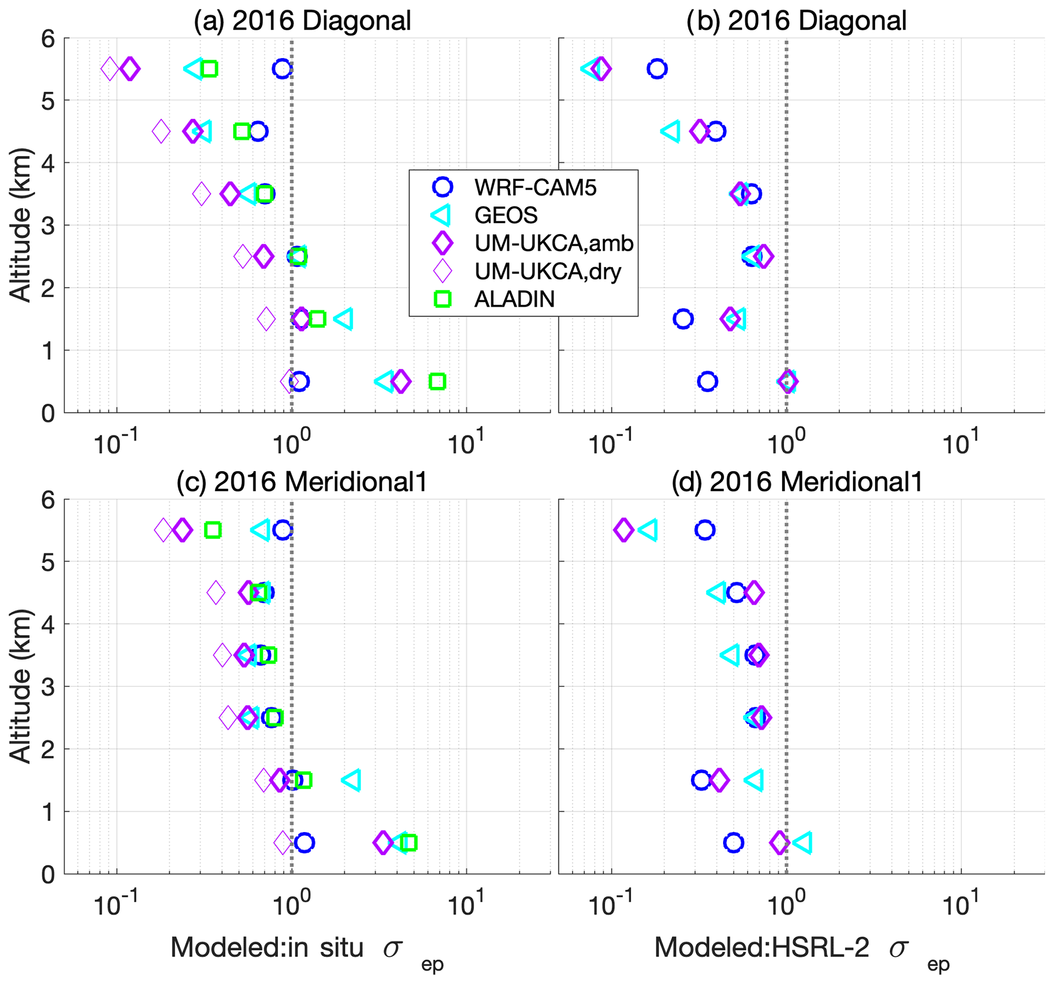
Figure 14 Mean ratio of modeled-to-in-situ low RH (a, c) and HSRL-2 ambient RH (b, d) mid-visible σ_ep across all grid boxes for the 2016 diagonal (a, b) and meridional 1 (c, d) comparison transects. Comparisons to both dry and ambient RH σ_ep are shown for the UM-UKCA model; for all other models, the comparison is to ambient RH σ_ep. The ratios for individual grid boxes, along with these means, are given in the Supplement (Fig. S15 for WRF-CAM5, Fig. S17 for GEOS, Fig. S19 for UM-UKCA, and Fig. S21 for ALADIN).

Shinozuka et al. (2020) estimated that, for September 2016, f(RH) was less than 1.2 for 90 % of the free troposphere aerosol measurements across the campaign. Estimates for the comparison grid boxes included here are consistent with this (Fig. S14) but also show that f(RH) for the 2016 diagonal grid boxes 3–6 in the 4–5.5 km altitude range were often higher, with means of 1.30±0.14, 1.46±0.19, 1.30±0.10, and 1.26±0.21 for grid boxes 3, 4, 5, and 6, respectively. Grid boxes farther north in the 2016 meridional 1 transect were also more humid, with f(RH) for grid boxes 1, 2, and 3 of 1.36±0.14, 1.39±0.14, and 1.44±0.51, respectively, in the 2–5 km altitude range. If γ is actually lower than derived here – e.g., closer to a value of ∼ 0.3, as measured in the year 2000 SAFARI campaign in southwestern Africa (Titos et al., 2016) – then the f(RH) values applied here would be about 30 % too large (∼ 1.5 vs. ∼ 1.2 for γ of 0.65 vs. 0.3 for an ambient RH of 60 %).

In both 2016 and 2017, RH at plume altitudes was generally <60 % (Figs. 10 and 11). In 2017, RH in the plume tended to decrease from the north (grid box 1) to the south (grid box 8) across the meridional 2 transect. The humidification factor f(RH) is accordingly estimated to decrease from typical values of 1.3–1.5 towards the northern end of the transect to 1.0–1.2 at the southern end (Fig. S14). In 2017, f(RH) is again slightly higher at 4–5 km altitude, and the humidity and f(RH) more variable than in the lower part of the plume. This is consistent with the fact that mid-level clouds were intermittently observed within and upwind of this transect.

In October 2018, the RH in the plume was greater than in September 2016 or August 2017 (Fig. 11 vs. Fig. 10) because convection was shifted further south and was carried over the SE Atlantic by the southern African easterly jet (Ryoo et al., 2021). It was still generally 60 % or lower in meridional 2 grid boxes 6–8, with f(RH) usually <1.3. North of this, in grid boxes 3–5, RH at 2–4 km was closer to 60 %, so f(RH) is more typically 1.3–1.5. In grid boxes 1 and 2, RH was closer to 80 % in the free troposphere. For these grid boxes, f(RH) was almost always greater than 1.5 and could exceed a factor of 2 (Fig. S14).

This analysis estimates the effect of humidification on light scattering only and not on light absorption. Since scattering dominates extinction, f(RH) for σ_sp nonetheless provides a good estimate of the impact of humidification on σ_ep. Based on this analysis, the in situ, low RH values of σ_ep are expected to typically be 20 %–50 % lower than the modeled and HSRL-2-measured ambient RH values of σ_ep, with everything else being equal. Instead, the modeled values of ambient RH σ_ep in the plume are generally lower than both the dry in situ values and the ambient RH HSRL-2 values.

WRF-CAM5

As for OA and BC, the observed σ_ep profiles are at a higher altitude and less vertically diffuse than in the models (Figs. 6–9). This produces a similar pattern to the biases in BC, OA, and σ_ep. The in situ measurements of σ_ep, in particular, increase more rapidly with altitude at the bottom of the plume and decrease more rapidly with altitude at the top of the plume than does the WRF-CAM5-modeled extinction. This is most pronounced in the grid boxes with higher concentration and/or more well-defined plumes (e.g., Fig. 6a). In addition, the observed plume is centered at a higher altitude than in the models. This leads to underestimates in modeled σ_ep in WRF-CAM5, relative to in situ values, in the core of the plume (3–4 km altitude) of about 30 %–35 % in 2016, 10 % in 2017, and 15 % in 2018 (Table 1; Figs. 14 and 15). Below and above the core of the plume (the 2–3 km and 4–5 km bins), the modeled-to-in situ-observed ratio in σ_ep is closer to 1.0. In 2017 and 2018, WRF-CAM5-modeled extinction at 5–6 km is more than 4 times (2017) and 9 times (2018) greater than that observed in situ (Fig. 15), but this is because σ_ep is measured to be near zero above 5 km in most grid boxes.

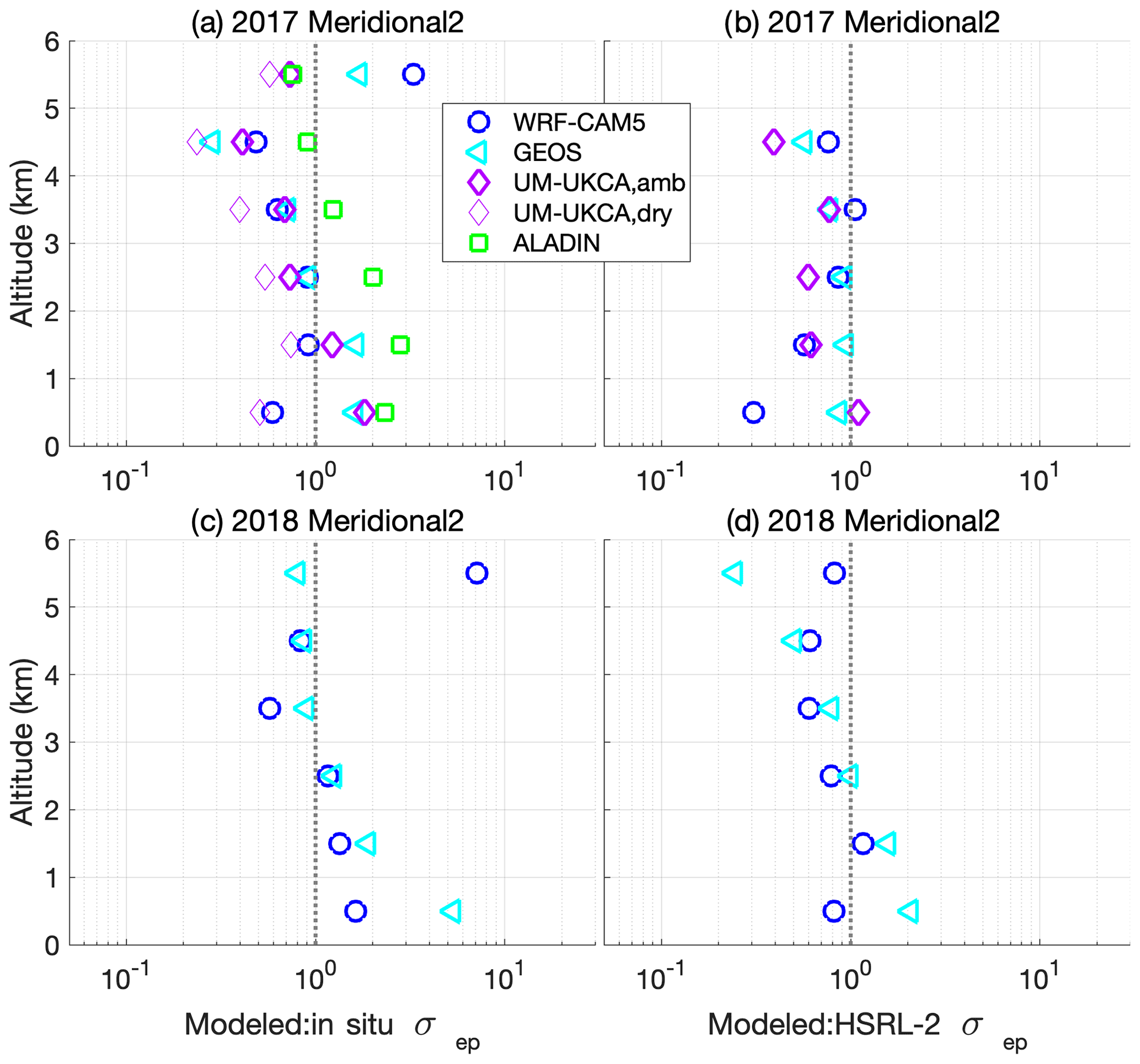
Figure 15 As in Fig. 14 but for the (a, b) 2017 and (c, d) 2018 meridional 2 comparison transects. The ratios for individual grid boxes, along with these means, are given in the Supplement (Fig. S16 for WRF-CAM5, Fig. S18 for GEOS, Fig. S20 for UM-UKCA, and Fig. S21 for ALADIN).

Biases in the model, when compared to σ_ep from HSRL-2, follow a similar but less consistent pattern (Figs. 14 and 15; Table 2). Again, the measurements show a plume core that is centered at a higher altitude and is less vertically diffuse than in the models, especially in 2016 (Fig. 8). The model mean low bias referenced to the HSRL-2 measurements is generally greater than the mean low bias compared to in situ observed σ_ep (compare Tables 1 and 2), consistent with the former being at ambient RH and the latter dry σ_ep. Except in the 2018 meridional 2 transect, WRF-CAM5 σ_ep is generally 30 %–40 % lower than measured by HSRL-2 (Table 2).

Table 2 As in Table 1 but for retrieved values of σ_ep only from the HSRL-2 lidar on board the ER-2 aircraft in 2016 and the P-3 aircraft in 2017 and 2018. Both modeled and observed values are at ambient RH. The modeled values are 550 nm, and the HSRL-2 values are at 532 nm.

Notable in comparing Figs. 6 and 8 is that, in 2016, when the HSRL-2 was on board the ER2 and so had retrievals to >6 km altitude, the top of the plume extends to higher altitudes than covered by the in situ measurements. In the latter, σ_ep drops to near zero above 6 km in most comparison grid boxes; in the HSRL-2 retrievals, σ_ep above 5.5 km is usually still >50 Mm⁻¹. The in situ and HSRL-2 measurements were not coincident, so this difference could simply reflect different sampling, but the consistency of this feature across multiple comparison transects makes this seem unlikely. Relative humidity often increased above about 4 km (Fig. 6), with humidification often amplifying σ_ep by a factor of 1.5 or more (Fig. S14). While this cannot fully account for the very large difference in σ_ep in the models versus that observed in situ, or all of the difference between the plume-top behavior between the in situ and HSRL-2 measurements, humidification differences could be contributing.

The net effect of these altitude-dependent biases in σ_ep is that WRF-CAM5 underestimates plume AOD, with Shinozuka et al. (2020) calculating a low bias of 10 %–30 % in AOD for the 2016 campaign. Here, the modeled ambient RH σ_ep is typically 70 %–80 % of the in-situ-measured dry σ_ep (with considerable variability). Accounting for the difference in humidity of the in situ measurements (i.e., scaling in situ σ_ep by 1.2–1.5) would make the WRF-CAM5 σ_ep in the plume to only about 50 %–70 % of the observed average. This is not far from the observed ratios of WRF-CAM5 to HSRL-2 observed ambient RH σ_ep (Table 2).

GEOS

Biases in GEOS-modeled σ_ep profiles have a strong vertical gradient in most comparison transects, with generally positive biases below about 2 km; above this, the model has a low bias that becomes greater with altitude (Figs. 14 and 15; Table 1). The low bias in GEOS σ_ep is smaller for August 2017 than for September 2016 and smaller again for October 2018. (Tables 1 and 2). In 2017, the bias also has a less consistent dependence on altitude (Fig. 15). In 2018, the higher ambient RH (Fig. 11) could be compensating for some of the low bias in dry aerosol σ_ep.

Overall, it is clear that GEOS underestimates σ_ep in the plume and centers the plume at too low an altitude (Figs. 6–9), with a net impact of underestimating the above-cloud AOD. This is consistent with the finding of a greater low bias in AOD from GEOS (30 %–50 %) than from WRF-CAM5 (10 %–30%) in Shinozuka et al. (2020). As for WRF-CAM5, accounting for humidification in the in situ observations would increase the estimated bias in GEOS to greater than a factor of 2. This is somewhat surprising, given that GEOS assimilates satellite-retrieved AOD every 3 h (Albayrak et al., 2013).

ALADIN

Statistics from the ALADIN model are not available for comparison to the HSRL-2-retrieved σ_ep, so comparisons are made to in situ σ_ep only. For both 2016 transects, ALADIN-modeled σ_ep is underestimated at the core of the plume, and the modeled plume is too vertically diffuse (Fig. 6). Also apparent is that the model increasingly places the plume at too low an altitude (Figs. 14 and 15), with the plume notably too low at the northwestern end of the diagonal transect (Fig. 6), consistent with too much subsidence in the model with aerosol transport (Das et al., 2017). In the 2016 diagonal transect, this produces a low bias in modeled σ_ep that increases with altitude from 3 to 5 km and high biases below 3 km (Fig. 14a; Table 1), which is much the same as for the GEOS model.

In 2017, biases in ALADIN-simulated σ_ep along the meridional 2 transect again have an altitude dependence, indicating a plume that is displaced too low in altitude, but in this case producing high biases below 4 km altitude (Fig. 15a). There is, in particular, a tendency for the model to overestimate σ_ep at the northern end of this transect and underestimate it at the southern end (Fig. S21), very possibly due to humidification amplifying σ_ep by about a factor of 2 for the northern grid boxes but only by a factor of ∼1.1–1.4 at the southern end (Fig. S14).

Notably, the ALADIN simulations were run using fixed 2014 GFED emissions. Central and southern African biomass burning emissions in 2014 were not particularly different from the 2001–2013 climatological average (Kaiser and Van der Werf, 2015). While not a direct measure of emissions, AOD over the SE Atlantic was lower in both September 2016 and August 2017 than the 2003–2018 average (Redemann et al., 2021), consistent with lower emissions in these months and years than on average. If the ALADIN simulations had used the emissions for the observed months, modeled σ_ep may have been smaller, with greater low biases in 2016 and greater high biases (below 4 km) in comparison to the observations.

UM-UKCA

For the UM-UKCA model, dry as well as ambient RH σ_ep values were reported, allowing for a more robust comparison to the measured low RH σ_ep and a rough comparison of observed versus modeled humidification factors. At all altitudes above 2 km, the model underpredicts dry aerosol σ_ep significantly across all comparison transects in 2016 and 2017 (Figs. 14 and 15; Table 1). This low bias increases systematically with altitude from 2 to 5 km. The grid box mean dry σ_ep is typically a factor of 2 to 3 lower in the model in the 3–4 and 4–5 km altitude bins than observed in situ. The altitude dependence of the model biases again results from the modeled plume being too vertically diffuse and the plume core too low in altitude.

Even with humidification added, the UM-UKCA-modeled extinction is lower than the observed dry σ_ep, despite the fact that the model aerosol appears to be too hygroscopic. In 2016, modeled σ_ep in the 2–5 km altitude range is a factor of 1.4 higher at ambient RH than for the dry aerosol; for 2017, it is a factor of 1.5 higher. These humidification factors are somewhat higher than expected from our analysis from the in situ observations, where f(RH) at these altitudes averaged 1.2 in both 2016 and 2017 (Fig. S14). The significant contribution of humidification to σ_ep also manifests in the fact that the modeled ambient RH σ_ep is typically 0.55–0.75 of that observed from the HSRL-2, and the simulated dry values of σ_ep are typically 0.2–0.5 of that observed in situ (Figs. 14 and 15; Tables 1 and 2).

The UM-UKCA low biases in dry σ_ep are much greater than the model low biases in OA and BC, indicating that the model has a low bias in biomass burning aerosol mass extinction efficiency and mass. There could also be simply less total aerosol mass (e.g., of components other than OA and BC, such as sulfate) in the UM-UKCA model than in reality.

4.3 Biases in aerosol intensive optical properties

Model biases in aerosol constituent component masses (BC and OA) and σ_ep can arise from a combination of biases in the emissions, transport, deposition, and (for OA) in-atmosphere production and loss from the aerosol phase of the biomass plume aerosol, which will clearly affect the magnitude of the calculated direct aerosol radiative effect. As noted earlier, the aerosol intensive optical properties, in particular the SSA, will also affect the sign of the aerosol DARE. The SAE connects the aerosol mass and extinction through the aerosol size, which is directly related to its aerosol mass scattering efficiency. The SAE and AAE, combined with mid-visible σ_ep, give the wavelength-dependence of SSA (Russell et al., 2010).

4.3.1 Single scatter albedo (SSA)

Observed and modeled SSAs differ in two respects, namely in their absolute value and in their variation with altitude. In September 2016, the observed SSA increases with altitude within the biomass burning plume along both the diagonal and meridional 1 transects (Fig. 16), generally increasing from 0.82–0.84 at the bottom of the plume to 0.86–0.88 at the plume top. In August 2017, SSA spanned a similar range as in 2016 (Fig. 17), but there is no significant gradient in SSA with altitude in the northern four meridional 2 grid boxes and only a slight indication of an increase in SSA with altitude towards the southern half of the plume. There is also no vertical gradient in SSA in the northernmost three meridional 2 grid boxes in October 2018, and SSA is overall higher than in September 2016 and August 2017.

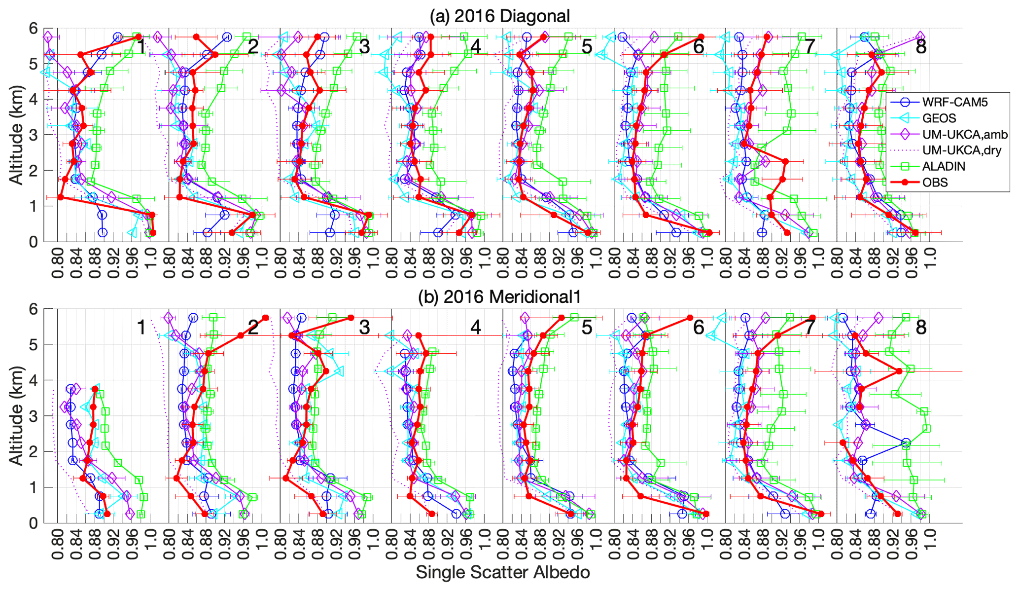
Figure 16 Profiles of SSA as observed (at low RH and 530 nm) and modeled (at ambient RH and also, for UM-UKCA, dry, at 550 nm) for the 2016 (a) diagonal and (b) meridional 1 transects.

A vertical gradient is apparent in the southern five meridional 2 grid boxes in 2018, where SSA increases from 0.86–0.89 at plume bottom to 0.90–0.92 at plume top. Notably, grid boxes 4–7 are located well within the biomass plume, whereas the northern end of this transect was often outside of or on the edges of the plume. The vertical gradient in SSA has been associated with a gradient in aerosol composition (Redemann et al., 2021). Accounting for this gradient is important in determining the direct aerosol radiative effect because it is the extinction-weighted column SSA, combined with below-plume albedo, which dictates the sign of the direct forcing.

WRF-CAM5 produces little to no associated gradient in SSA with altitude (Figs. 16 and 17), showing increases in SSA only at the very top of the plume in some comparison grid boxes. Within the plume, modeled SSA encompasses quite a small range, which is almost always 0.82–0.84 in the September 2016 transects and the August 2017 transect (Fig. 15). This difference in vertical gradient explains why Shinozuka et al. (2020) find greater low biases in the 3–6 km altitude column SSA than in the lower free troposphere column SSA. As in the observations, in October 2018 the WRF-CAM5 SSA is slightly higher than in the other years, generally 0.84–0.86. WRF-CAM5 does not consider OA and BC aging, and primary OA hygroscopicity is low (0.1), which is consistent with the small range in SSA.

Figure 17 As in Fig. 16 but for the (a) 2017 and (b) 2018 meridional 2 transects.

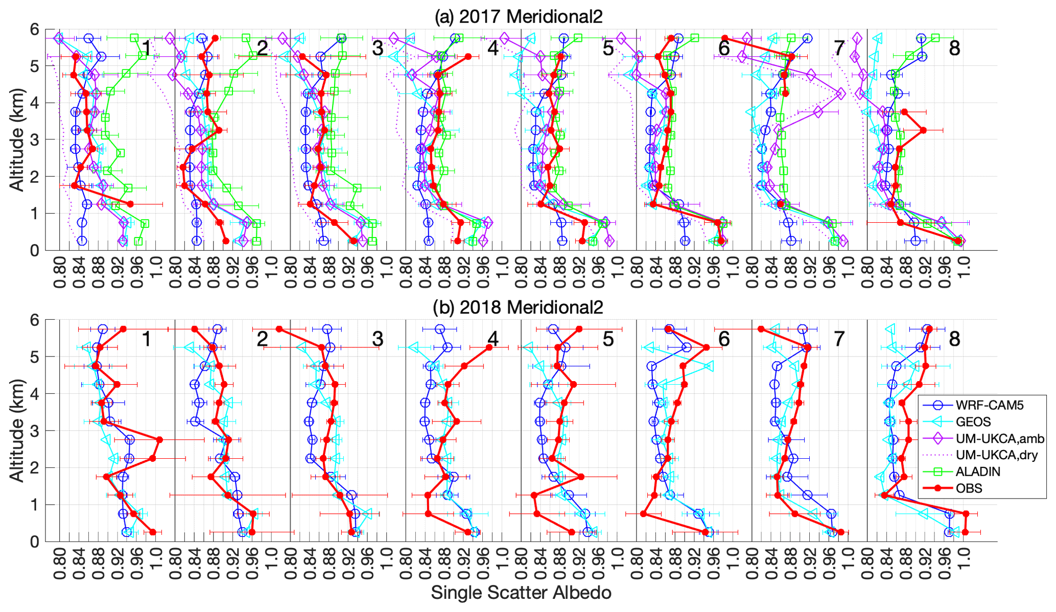
GEOS, similarly, has little gradient in SSA with altitude within the plume, and, where it does, the tendency is for SSA to decrease with altitude, particularly towards the plume top. Here it diverges from the observed, increasing dry aerosol SSA. Mean plume SSA values, on average, are similar in GEOS and WRF-CAM5, but SSA is about twice as variable in GEOS. This larger range in SSA does not show any apparent spatial pattern, other than having somewhat higher SSA in the northernmost meridional 2 grid box in both 2017 and 2018. This grid box tended to be either on the northern edge or out of the main biomass burning plume. Aging of OC in GEOS could be creating more hygroscopic aerosol with time, which, in turn, would increase the variability in ambient SSA through differences in water uptake.

In the UM-UKCA simulations, SSA decreases significantly towards the top of the plume in some comparison grid boxes. In most cases this is true for both the dry and ambient RH aerosol SSA, so this appears to be driven by a change in aerosol composition or size but not by, e.g., a decrease in scattering due to a decrease in RH. The UM-UKCA ambient RH SSA values are within 0.02 of the values measured in situ at most altitudes in the plume (Fig. 14), but the dry aerosol SSA from UM-UKCA is significantly lower (typically 0.77–0.83) than both the modeled ambient RH values (typically 0.84–0.88) and the dry in situ values (Figs. 16 and 17). This difference between the SSA of the dry and ambient RH aerosol results from the significant increase in extinction with RH (Sect. 4.3.2).

ALADIN is the only model of the four where the SSA (which is at ambient RH) has a similar gradient with altitude in the plume to that observed. SSA in ALADIN includes a dependence on aerosol aging and RH (Mallet et al., 2019), and thus, it is not clear if this altitude dependence in SSA is a response to higher RH towards the top of the plume or if it would still be present under dry conditions. ALADIN-modeled SSA is also consistently higher than that observed.

The observed values of SSA are available only at low RH since σ_ap was measured only at low RH, and only the UM-UKCA model provided both dry and ambient RH values of SSA. This makes it difficult to determine how much humidification differences are contributing to the differences between the observed and modeled SSA. The models include the effect of humidification on SSA by accounting for the impact of water on the aerosol indices of refraction (WRF-CAM5, GEOS, and UM-UKCA) or by parameterizing the effect of RH on SSA (ALADIN; Mallet et al., 2017, 2019). In all four models, the result is an increase in SSA with humidification. In reality, it is likely that humidification affects both scattering and absorption. However, the former has been well quantified observationally, whereas the latter has not and is therefore highly uncertain (e.g., Bond et al., 2013; Zhou et al., 2020).

The modeled ambient RH SSA at plume altitudes is generally lower than the observed dry aerosol SSA in both the WRF-CAM5 and GEOS models (Fig. 18). Thus, the dry aerosol SSA in these models has an even greater low bias than indicated by Figs. 14–16; whether it is as large as the low bias in the UM-UKCA dry SSA depends on the relative effects of humidity on scattering and absorption in the models. Humidity in the plume was somewhat higher in August 2017, and, in particular, October 2018 than in September 2016 (Fig. 11 versus Fig. 10), thus increasing modeled SSA and moving the modeled (ambient RH) and observed (dry) SSA values in closer alignment on average. In contrast, for the two 2016 transects, the ALADIN ambient RH SSA is almost always higher than the observed dry SSA, with typical differences of 0.02–0.04. Adjustment of the ALADIN (ambient RH) values to low RH (as in the observations) should bring the two into better agreement, though perhaps not for all transects. The differences are smaller in the 2017 meridional 2 transect, particularly towards the south, despite the higher ambient RH.

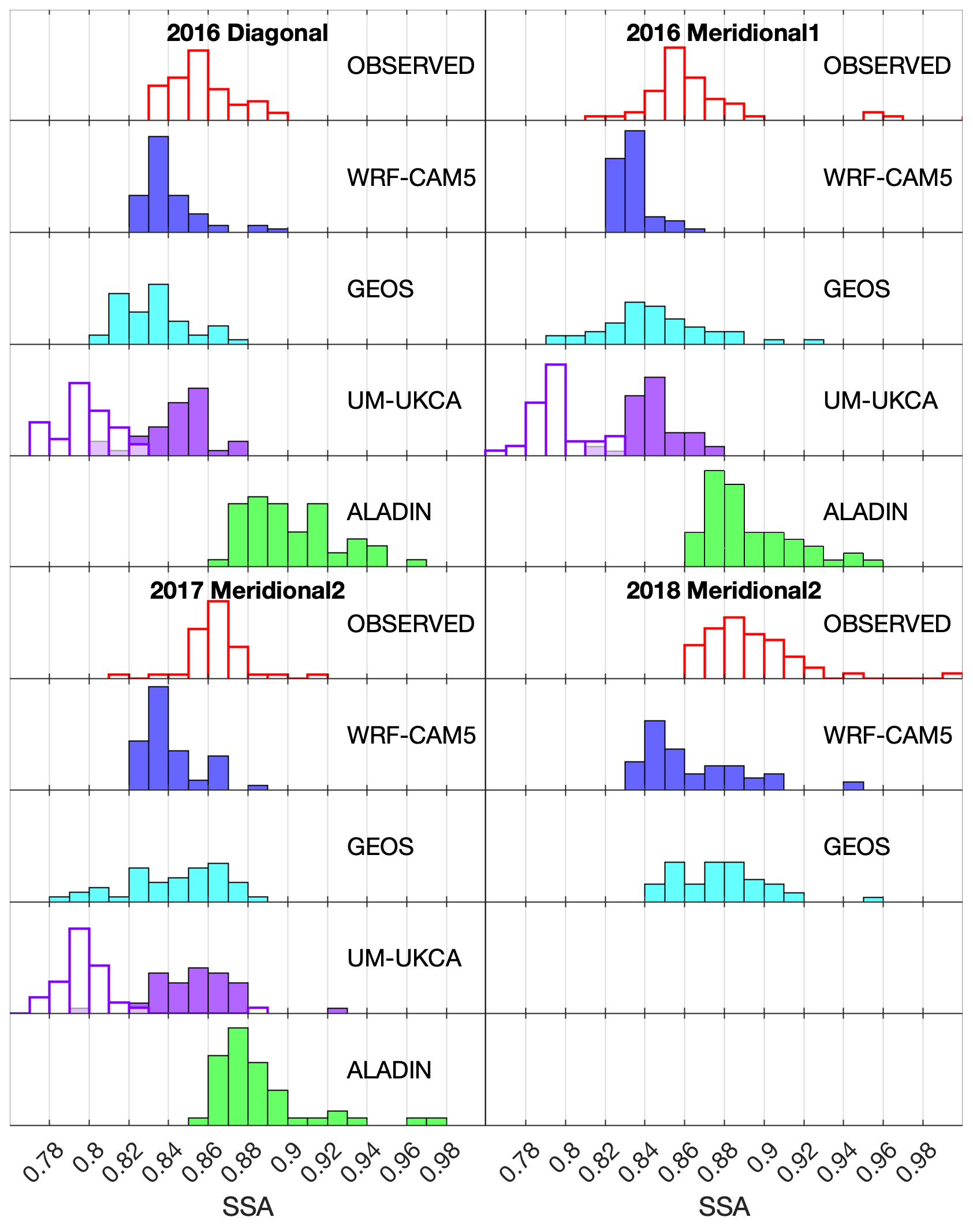
Figure 18 Histograms of SSA from the 2–5 km altitude range only, as measured in situ from the P-3 and as modeled using WRF-CAM5, GEOS-5, UM-UKCA, and ALADIN for all samples along the comparison transects. For the UM-UKCA model, values are shown for both ambient RH aerosol (filled bars) and dry aerosol (unfilled bars); the observed values are available only for the dry aerosol (unfilled bars).

Aerosol SSA is determined largely by aerosol composition which, for biomass burning aerosol, is dominated by organic aerosol (e.g., see Fig. 14 of Redemann et al., 2021). Black carbon is highly absorbing, so the mass fraction of BC in particular drives SSA. As discussed below (Sect. 6), the relative biases in OA and BC indicate that the models have a higher OA:BC ratio than observed. For given indices of refraction for these components, a higher OA:BC ratio would increase SSA in the models (since they do not include organic aerosol brown carbon absorption). Thus, the model OA:BC ratio does not explain the low bias in SSA in the WRF-CAM5 and GEOS models. Biases in model aerosol component indices of refraction, photochemical whitening (Carter et al., 2021), incorrect representation of the impacts of internal mixing on indices of refraction, and the influence of aerosol components other than BC and OA could all be contributing to the observed modeled biases in SSA.

An earlier study using data from the ORACLES 2016 field season compared SSA derived from the in situ measurements used here and from three remote sensing instruments (Pistone et al., 2019). These were a spectral radiometer (SSFR) in combination with Sun-photometer-derived AOD, a hyperspectral Sun photometer and sky radiometer (4STAR) in combination with SSFR-derived scene albedo, and an imaging polarimeter (Airborne Multi-angle Spectro Polarimetric Imager – AirMSPI). The SSFR and 4STAR instruments were deployed on the NASA P-3 aircraft along with the in situ instruments; the AirMSPI instrument was mounted on the NASA ER-2 high-altitude aircraft which overflew the P-3 at least once on coincident flight days (see Pistone et al., 2019, for more detail). The remote sensing instruments, like the models, all derive SSA at ambient RH. At 530 nm, the average distribution of SSA from the in situ instruments was higher than the 4STAR SSA by (on average) 0.01–0.02 (with 10–90 percentile ranges of 0.07 in each) but was generally lower than the AirMSPI SSA, with differences of 0.03, with less variability overall (0.03 in 10–90 percentiles) compared with the P-3 instruments. The spread in differences was likely in part due to the full campaign measurements not being coincident in either time or space due to the varying measurement techniques. Direct comparison to the SSFR was made in one case study only, and for that case, the SSFR 530 nm SSA was <0.01 lower than the in situ SSA (within the instrument uncertainty ranges). These results indicate it is unlikely that SSA from the in situ instruments is significantly biased high. It also supports the idea that humidification is not significantly influencing SSA over the SE Atlantic, since the in situ values are at low RH, and the remote sensing values are at ambient RH. They also imply that the impact of humidification on SSA in the UM-UKCA model (Fig. 18) is too large (consistent with f(RH) being too large; see the subsection on ALADIN), though it is difficult to make a robust conclusion based on this one observational comparison.

4.3.2 Scattering Ångström exponent (SAE)

Whereas SSA varies primarily with aerosol composition, SAE varies primarily with aerosol size. For aerosol smaller than approximately 1000 nm in dry diameter – i.e., as for aerosol in the SE Atlantic biomass burning plume (Shinozuka et al., 2020) – SAE becomes smaller as aerosol size increases (Schuster et al., 2006). The observed SAE is quite consistently 1.7–1.9 within the plume, with very little vertical variation or difference across the 2 campaign years (2016 and 2017) where observations are available (Figs. 19 and 20). WRF-CAM5-simulated SAE deviates the furthest from the observed values, with values in the plume generally 0.9–1.3, which is consistent with the larger aerosol size in WRF-CAM5 than in reality (see Fig. 4 in Shinozuka et al., 2020). GEOS and UM-UKCA both reproduce the observed SAE quite well, with the exception of a few grid boxes. The GEOS SAE values are typically 0.1–0.2 smaller than observed in the 2016 meridional 1 grid boxes 1–3 and above about 4 km at the northern end of the 2017 meridional 2 transect. Both the dry and ambient RH UM-UKCA values of SAE generally agree well with the observed SAE, which consistent with the UM-UKCA aerosol being only slightly larger than observed.

Figure 19 As in Fig. 16 but for the scattering Ångström exponent (SAE).

Figure 20 As in Fig. 17 but for the scattering Ångström exponent (SAE).

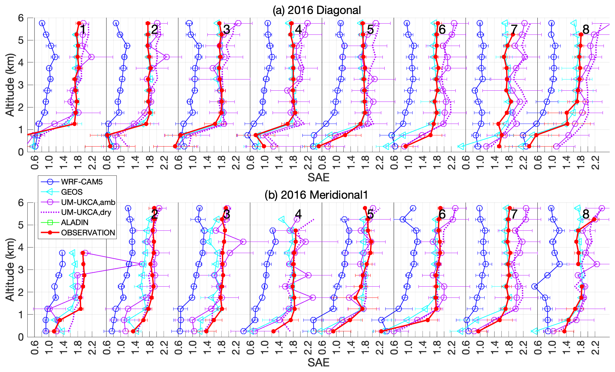
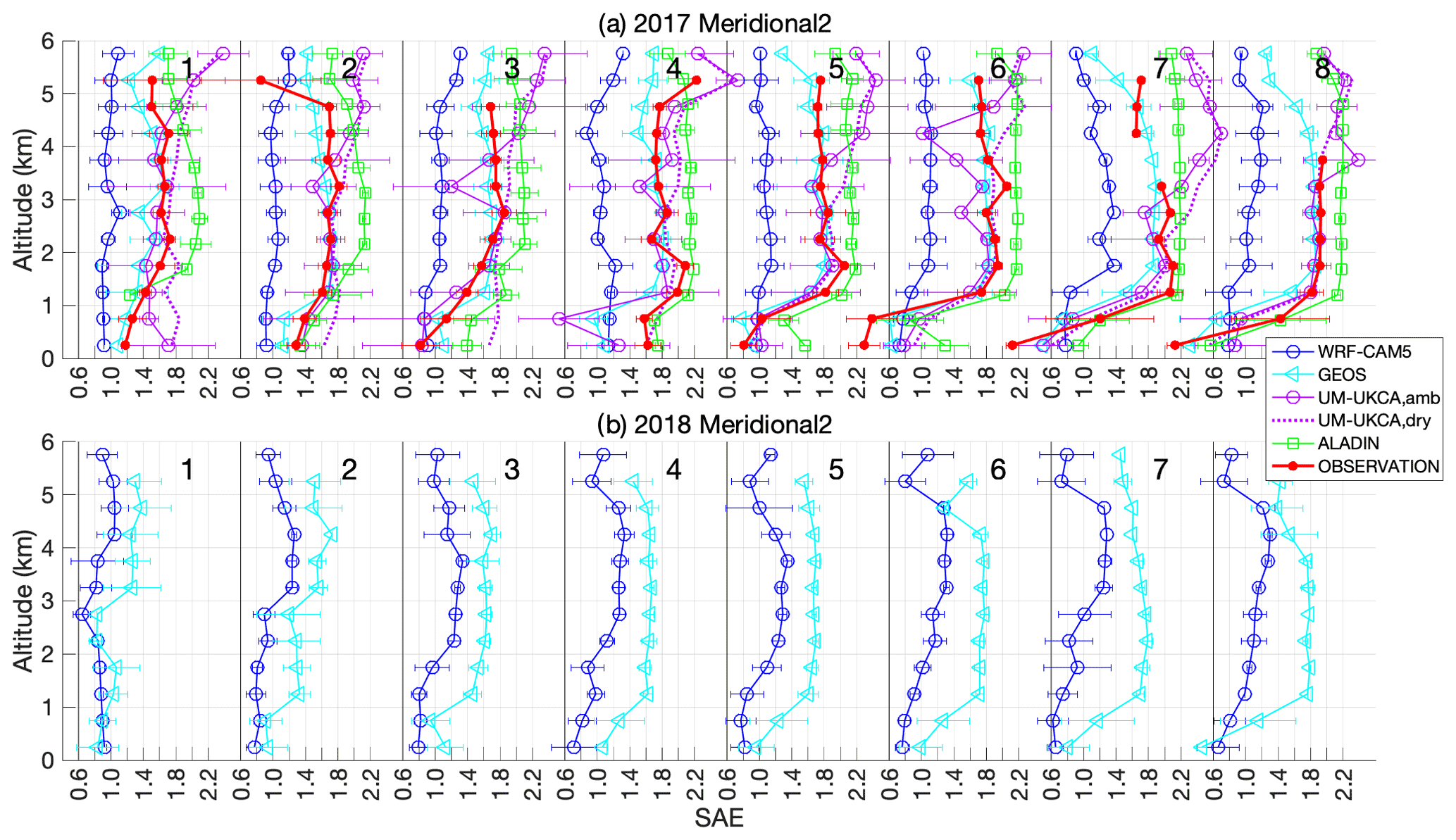
Both GEOS and UM-UKCA simulate vertical gradients – but of opposite sign – in SAE, and a gradient is not present in the observations. The ALADIN model also has a less-pronounced decrease in SAE towards the top of the plume, and it simulates SAE values that are typically 0.02–0.04 higher than what are observed in almost all grid boxes and plume altitudes. This is consistent with the aerosol in ALADIN being smaller than the observed aerosol, but the model uses a bulk bin scheme, so a mean aerosol size is not available for comparison. The GEOS and ALADIN models do include the effect of aging on aerosol hygroscopicity, possibly driving the modeled gradients in SAE.

The very small difference between the UM-UKCA simulated dry and ambient RH aerosol SAE values are surprising, given the large between difference dry and ambient RH-simulated σ_ep (see the subsection on UM-UKCA) and SSA (Figs. 16–18). The relative changes in σ_ep and SSA with humidification in this model are consistent with the change in SSA being driven by an increase in light scattering alone, e.g., an increase in σ_sp of a factor of 1.45 – which is the mean f(RH) for σ_ep in the UM-UKCA model in the 2016 transects (see the subsection of ALADIN) – would produce a change in SSA from 0.80 to 0.85, which is consistent with the increase in SSA with humidification in the model (Fig. 18). This implies significant aerosol growth with humidification, which should be reflected in the SAE. Resolving this apparent inconsistency would require work outside of the scope of this paper that considers more carefully the simulated size distribution and size-dependent composition of the aerosol.

4.3.3 Absorption Ångström exponent (AAE)

As noted above, the in situ PSAP measurements of σ_ap at 530, 460, and 660 nm are processed using two sets of correction factors, namely wavelength averaged and wavelength specific (Virkkula, 2010). The two are nearly identical at 530 nm but differ at 460 and 660 nm and so produce quite different values of the absorption Ångström exponent, both versions of which are shown in Figs. 21 and 22. In the 2–5.5 km altitude range, the wavelength-independent correction factors yield AAE values of 1.2±0.1 in 2016 and 1.1±0.2 in 2017 and 2018. AAE at these same altitudes calculated with the wavelength-specific correction factors are about 0.3–0.4 higher, with average values of 1.5±0.1 in 2016 and 1.5±0.2 in 2017 and 2018.

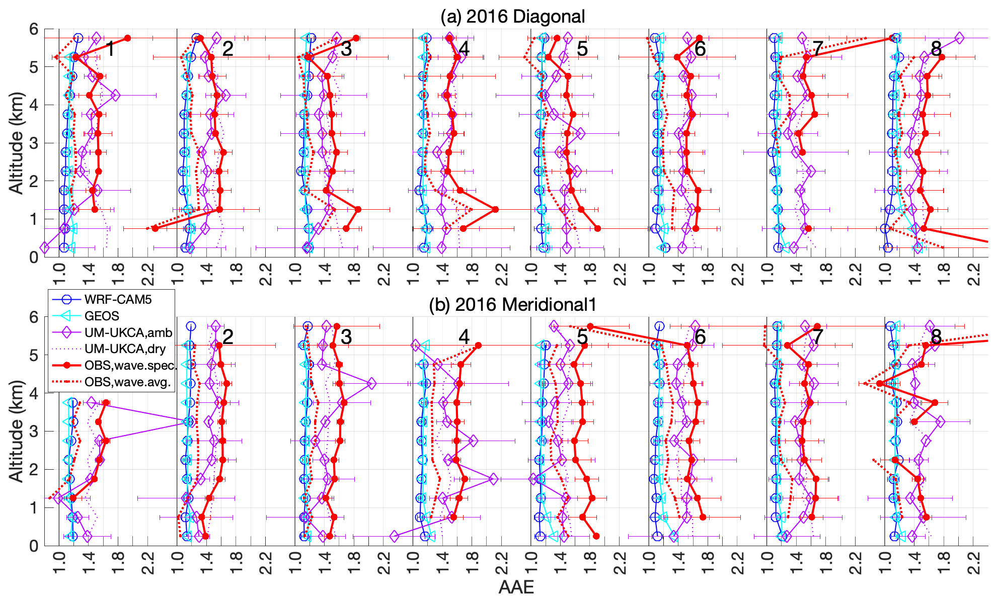
Figure 21 As in Fig. 16 but for the absorption Ångström exponent (AAE). Observed values of AAE are given for both the wavelength-specific and wavelength-averaged correction factors.

Figure 22 As in Fig. 17 but for the absorption Ångström exponent (AAE).

The Pistone et al. (2019) comparison of spectral SSA across different instruments during ORACLES 2016 used SSA calculated from σ_ap using the wavelength-averaged correction factor. Using the wavelength-specific correction factors produces higher 470 nm absorption, with the result that SSA is lower at both 470 and 660 nm than at 530 nm (Pistone et al., 2019). In contrast, SSA derived from absorption using the wavelength-averaged correction factors decreases with wavelength. The latter agrees better with the shape of the spectral SSA from the remote sensing instruments, indicating the lower values of AAE (derived from σ_ap values using the wavelength-averaged correction) are more likely to be correct. Values of AAE close to 1 are consistent with the absorption being dominated by black carbon (Bergstrom et al., 2007; Bond et al., 2013), so if these lower values are correct, then there is likely little brown carbon absorption, as also indicated by other recent studies of biomass smoke in the SE Atlantic (Chylek et al., 2019; Denjean et al., 2020; Taylor et al., 2020). These four models simulate both black and organic carbon, but the organic carbon is not light-absorbing, so AAE values are expected to be near 1. They do include the impacts of the addition of water on the aerosol indices of refraction and aerosol size, which can drive variations in AAE from black carbon alone (i.e., of about 0.8–1.4; Liu et al., 2018).

AAE from the WRF-CAM5 and GEOS models are significantly lower than the in situ wavelength-specific values and are slightly, but not significantly, lower than the wavelength-independent values (Figs. 21 and 22). In both models, AAE in the 2–5.5 km altitude range is 1.1 in 2016 and 2017 and 1.2 in 2018, with standard deviations of <0.05. The UM-UKCA AAE values vary from the observed values but, on average, are in good agreement with the in situ AAE derived using the wavelength-specific correction factors.

4.4 Biases in cloud fraction and cloud optical thickness

Observed cloud properties are retrieved from satellite observations and are available from every day of the three field campaign periods and for the zonal transect as well as for the diagonal, meridional 1, and meridional 2 transects. Mean CF_warm and geometric mean COT_warm from the satellite retrievals are compared to model averages across all daytime hours (Figs. 23–25). We treat the SEVIRI-LaRC retrievals as the benchmark for CF_warm, since these measurements cover the daytime hours, and the MODIS-ACAERO retrievals are treated as our benchmark for COT_warm, since they account for the effects of absorbing aerosol above the clouds, while acknowledging that any satellite retrievals of clouds may be subject to systematic biases. In cumulus cloud regions in particular, 3D radiative effects and subpixel clear-sky contamination may bias the retrieved values of COT_warm to be low (e.g., Marshak et al., 2006; Kato et al., 2006; Painemal et al., 2013), whereas the coarse pixel resolution relative to the cloud size could yield an overestimation of CF_warm (e.g., Zhao and Di Girolamo, 2006).

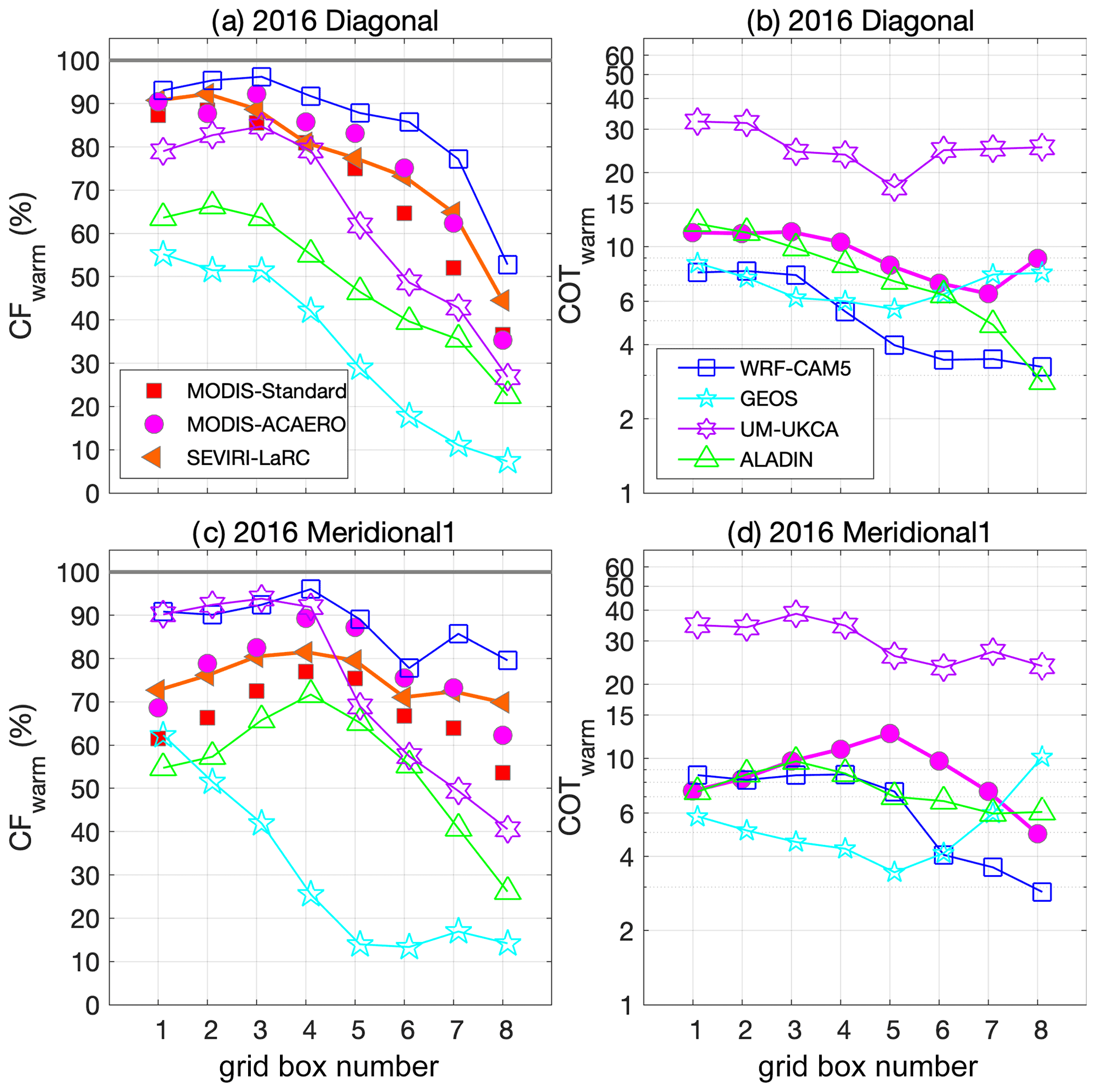
Figure 23 Average daytime mean CF_warm (a, c) and COT_warm (b, d) from satellite retrievals and from the models for the comparison grid boxes in the 2016 diagonal (a, b) and meridional 1 (c, d) transect. COT_warm is the geometric mean, except for the ALADIN model, which shows the median. The SEVIRI-LaRC dataset is used as the reference for observed CF_warm, and the MODIS-ACAERO dataset is used as the reference for observed COT_warm in the comparison to models.

Figure 24 As in Fig. 23 but for the 2017 (a, b) and 2018 (c, d) meridional 2 transects.

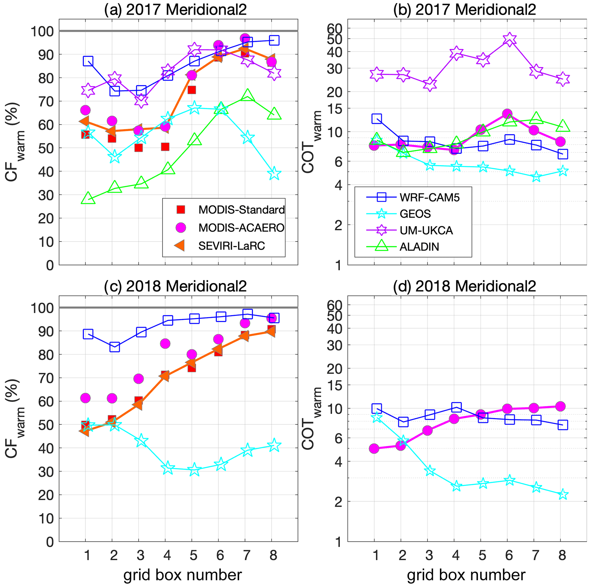
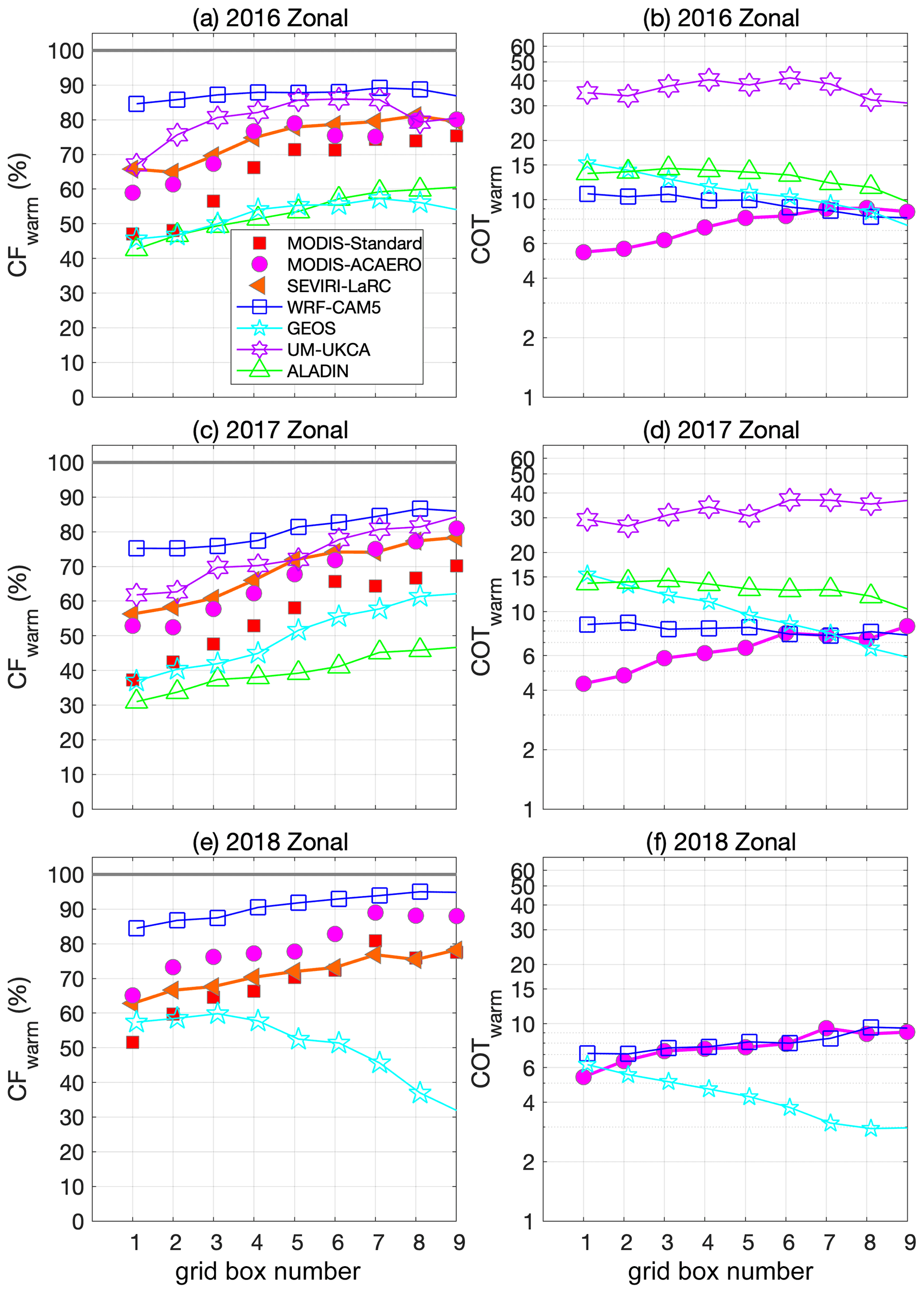
Figure 25 As in Fig. 23 but for the zonal transects in 2016 (a, b), 2017 (c, d), and 2018 (e, f).

The observed CF_warm from all three satellite data products is quite high (> 60 %–70 %) across almost all comparison transect grid boxes, except at the southeastern end of the diagonal transect in 2016 (Fig. 23). Differences in the observation times of the MODIS and SEVIRI instruments are expected, on average, to lead to CF_warm values that are about 1 %–10 % lower for the two MODIS products (Sect. 3.2.3 and Table S2), but in our statistics, CF_warm from MODIS standard and MODIS-ACAERO are not always lower than from SEVIRI-LaRC (Figs. 23–25). Differences in the spatial resolution (3 km for SEVIRI; 1 km for MODIS), in the algorithms used for identifying warm clouds, and in the aggregation of statistics (e.g., the L2 datasets for MODIS-ACAERO versus the L3 dataset for MODIS standard) could also be producing differences in derived CF_warm. Notably, the uncertainty in the true CF_warm, as expressed through the differences between the satellite products, is much lower than the differences between CF_warm from the observational datasets and the models.

CF_warm in WRF-CAM5 is higher than in all three observational datasets (Figs. 23–25). This is particularly the case in regions of low cloud fraction, so the gradients in cloud fraction across the transects follow the tendency of the observed gradients but are much smaller in magnitude. In contrast, the GEOS and ALADIN models both significantly underestimate CF_warm in all transects and almost all grid boxes. CF_warm gradients in the ALADIN model also track the observed gradients well but at a much lower cloud fraction. The GEOS model, in addition to significantly underestimating CF_warm, fails to capture the correct gradient in cloud fraction. In particular, the latitudinal gradient in the cloud fraction along the meridional 2 transect in both 2017 and 2018 is the inverse of that observed. The UM-UKCA model comes closest to the observed cloud fractions, with variable biases depending on the transect and grid box. Like WRF-CAM5, UM-UKCA biases in cloud fraction are largest where it fails to capture spatial gradients in cloud fraction, e.g., along the meridional 1 transect, at the northern end of the meridional 2 transect, and at the eastern end of the zonal transect.

In the SE Atlantic, the large-scale gradients in day-to-day cloud fraction are controlled by a number of different intertwined factors, including gradients in sea surface temperature (SST) from the Benguela current off the Namibian–Angolan coast and by lower tropospheric stability (Wood, 2012). Increases in CF_warm in the SE Atlantic have been shown to be correlated with increases in lower tropospheric stability (LTS), surface wind speed, and RH at 950 hPa (Fuchs et al., 2018). Seasonally dependent factors can also affect the SE Atlantic low cloud fields. In September, the intrusion of mid-latitude disturbances to lower latitudes can significant perturb the low clouds, reducing CF_warm. Elevated humidity in the free troposphere in October 2018 would also help reduce cloud-top entrainment drying. In the models, failure to capture these features and the dynamics that drive one or more of these variables could be the cause of incorrect gradients in CF_warm.

Differences in the representation of small-scale turbulent mixing processes and microphysics have been shown to hamper model skill in representing stratocumulus properties, even when large-scale forcings are fixed (Zhu et al., 2005; Wyant et al., 2007). Accurate prediction of cloud cover is complicated because the relative roles of different large-scale forcings varies across the region (Fuchs et al., 2018). During the 3 years of the ORACLES campaign, the SSTs were warmer than the climatological average, though this does not appear to have resulted in a significant impact on cloud fraction in the month-long averages (Ryoo et al., 2021).

Disentangling the sources of model biases in COT_warm are even more difficult, especially since COT_warm may be affected not only by thermodynamic processes but is also very sensitive to cloud microphysical process representation (Wyant et al., 2007) and to aerosol–cloud interactions. As discussed above, the models tend to place the smoke plume at lower altitudes than observed and, therefore, to mix more of the plume into the boundary layer and low clouds than is observed. This would lead to higher aerosol loadings in the boundary layer, higher cloud droplet number concentrations, and possibly higher COT_warm (assuming cloud liquid water path is not significantly reduced in response; Twomey, 1977). An exception is for the ALADIN model COT_warm, as aerosol microphysical effects on clouds were not simulated. Diagnosing the possible magnitude of this effect on COT_warm in the other models is beyond the scope of this paper.

The observed (MODIS-ACAERO) geometric mean COT_warm covers a fairly small range, of 8.3±1.8, across all transects and years (Figs. 23–25). WRF-CAM5 COT_warm values (8.1±1.9) are very similar to the observed values on average but deviate from the observed values by not capturing spatial gradients. The result is that WRF-CAM5 sometimes overestimates and sometimes underestimates COT_warm. ALADIN generally reproduces the observed COT_warm well, except at the western end of the zonal transect where COT_warm is about twice that observed. GEOS COT_warm is both too small and more spatially variable than observed (6.6±3.2); like CF_warm, the model also does not capture the correct spatial gradients in COT_warm. UM-UKCA significantly overestimates COT_warm across all transects, averaging 32.6±6.4.

It has been noted that global models tend to have a “too few, too bright” bias for low-level marine clouds (Nam et al., 2012). Here, none of the four models fit this paradigm, including the two global models (GEOS and UM-UKCA). The regional WRF-CAM5 model has too many clouds, but the clouds are of about the right brightness, the regional ALADIN model has too few clouds that are generally not bright enough but are sometimes too bright, clouds in the global GEOS model are both too few and not bright enough, and the global UM-UKCA model has too many clouds that are much too bright.

In reality, it is expected that COT_warm will tend to increase with CF_warm, and this is seen in the MODIS-ACAERO retrievals (Eq. 1 and Fig. S3). In contrast, the WRF-CAM5, GEOS, and ALADIN simulations show no significant change in COT_warm with CF_warm, so as the cloud field develops to produce greater coverage, the clouds are not becoming optically thicker. The range in CF_warm covered by the models across the comparison transects included here is smaller than in the observations; a question is whether COT_warm would remain largely invariant for CF_warm of 0–1.0 in the models. If so, COT_warm at lower cloud fractions would be too high in WRF-CAM5 and too low in GEOS and ALADIN. In contrast, in the UM-UKCA simulations COT_warm does increase with CF_warm at approximately the same rate as in the MODIS-ACAERO observations, but COT_warm is systematically too high (Fig. S3).

5 Impact of aerosol and cloud biases in the direct aerosol radiative effect

In order to quantify the net effect of model biases on the direct aerosol radiative effect (DARE), a first-order DARE estimate is calculated using the grid box mean aerosol and cloud properties for five of the comparison grid boxes. The 2016 diagonal grid box 3 was selected for being closer to the center of the plume while (in contrast to grid boxes 1 and 2) having more robust sampling (Figs. 1 and 2); in 2016 meridional 1 grid box 2 and 2017 and 2018 meridional 2 grid box 5 were selected for being located closer to the center of the plume meridionally; and in 2017 meridional 2 grid box 2 was selected in order to have one grid box with lower cloud fraction (57 %) since the other four selected grid boxes all have an average CF_warm of >75 %.

Following Haywood and Shine (1995), DARE at the top of the atmosphere can be estimated as follows:

$$\begin{array}{}\text{(2)}& \begin{array}{rl}\mathrm{DARE}& \approx -D\cdot S_o\cdot T_{\mathrm{at}}^{\mathrm{2}}\cdot \left(\mathrm{1}-A_{\mathrm{c}}\right)\cdot \mathrm{SSA}\cdot \overline{\mathit{\beta }}\cdot \mathrm{AOD}\\ & \cdot \left({\left(\mathrm{1}-R_{\mathrm{s}}\right)}^{\mathrm{2}}-{\displaystyle \frac{\mathrm{2}{R}_{\mathrm{s}}}{\overline{\mathit{\beta }}}}\left({\displaystyle \frac{\mathrm{1}}{\mathrm{SSA}}}-\mathrm{1}\right)\right),\end{array}\end{array}$$

where D is the daylight fraction of the day, S_o is the solar constant, T_at is the atmospheric transmissivity (absent aerosol), A_c is cloud fraction, SSA is the single scatter albedo, R_s is the surface reflectance, $\overline{\mathit{\beta }}$ is the spectrally weighted aerosol hemispheric backscatter fraction, and AOD is the aerosol optical depth. This formulation assumes zero forcing in the presence of clouds (since for A_c=1, DARE is equal to 0). The goal here is to calculate the forcing for an aerosol plume that, when clouds are present, is fully above the cloud layer and, therefore, has non-zero forcing. Equation (2) is therefore modified to the following:

$$\begin{array}{}\text{(3)}& \begin{array}{rl}\mathrm{DARE}& \approx -D\cdot S_o\cdot T_{\mathrm{at}}^{\mathrm{2}}\cdot \mathrm{SSA}\cdot \overline{\mathit{\beta }}\cdot \mathrm{AOD}\\ & \cdot \left({\left(\mathrm{1}-{\mathit{\alpha }}_{\mathrm{s}}\right)}^{\mathrm{2}}-{\displaystyle \frac{\mathrm{2}{\mathit{\alpha }}_{\mathrm{s}}}{\overline{\mathit{\beta }}}}\left({\displaystyle \frac{\mathrm{1}}{\mathrm{SSA}}}-\mathrm{1}\right)\right),\end{array}\end{array}$$

where α_s is the scene albedo below the aerosol plume, and AOD is the above-cloud AOD. In this formulation, the impact of clouds on DARE is accounted for through their effect on α_s. This DARE estimate does not account for the fact that the cloud fields (and, therefore, α_s) might have been affected by rapid adjustments to the smoke plume direct forcing (the semi-direct effect). Depending on the amount and altitude of heating by aerosol absorption above the clouds, this could have increased or decreased α_s, thereby affecting the calculation of DARE using Eq. (3).

DARE is nonlinear with α_s (Eq. 3 and Cochrane et al., 2021), so here DARE is calculated separately for clear (DARE_clear) and cloudy (DARE_cloudy) skies. The grid-box-averaged DARE (DARE_avg) is the sum of the two, which are weighted by their average fractional contributions in each grid box as follows:

$$\begin{array}{}\text{(4)}& \begin{array}{rl}{\mathrm{DARE}}_{\mathrm{avg}}& ={\mathrm{DARE}}_{\mathrm{clear}}\left(\mathrm{1}-{\mathrm{CF}}_{\mathrm{warm}}\right)\\ & +{\mathrm{DARE}}_{\mathrm{cloudy}}{\mathrm{CF}}_{\mathrm{warm}}.\end{array}\end{array}$$

This assumes that the aerosol is not systematically different over clear skies than over cloudy skies, as demonstrated for this region by Kacenelenbogen et al. (2019). The observed values of CF_warm used in Eq. (4) are the grid box means from the SEVIRI-LaRC retrievals.

For clear skies, α_s in Eq. (3) is set to 0.07 (approximated from Li et al., 2006, for ocean reflectivity), and for cloudy skies, α_s is the grid-box-averaged cloud albedo. The two-stream approximation of Feingold et al. (2017) is used to calculate the visible cloud albedo α_c as follows:

$$\begin{array}{}\text{(5)}& {\mathit{\alpha }}_{\mathrm{c}}={\displaystyle \frac{\frac{(\mathrm{1}-g)}{\cos {\mathit{\theta }}_o}{\mathit{\tau }}_{\mathrm{c}}}{\mathrm{2}+\frac{(\mathrm{1}-g)}{\cos {\mathit{\theta }}_o}{\mathit{\tau }}_{\mathrm{c}}}},\end{array}$$

where the asymmetry factor, g, is set to 0.85 (Bohren, 1980), the solar zenith angle, θ_o, is fixed at 30^∘, and cloud optical thickness, τ_c, is set to the grid box log-mean value of COT_warm from the MODIS-ACAERO retrievals.

In Eq. (3), D is fixed at 0.5 (which is correct to within 0.02 for this latitude range in all 3 months), S_o is set to 1361 Wm⁻² (Kratz et al., 2020), and T_at is set to 0.79, based on Fig. 1 of Wild et al. (2019). The value $\overline{\mathit{\beta }}$ is calculated using Eq. (11b) of Reid et al. (1999), which parameterizes $\overline{\mathit{\beta }}$ as a function of σ_ep at 550 nm and the extinction Ångström exponent (EAE) across 437–669 nm (close to our wavelength span of 470–660 nm) for biomass burning smoke. For the grid boxes included in this analysis, modeled $\overline{\mathit{\beta }}$ values varied from a low of 0.094 (in WRF-CAM5) to a high of 0.159 (in ALADIN), with observed values in the range 0.11–0.13 (Table 3). EAE, used in deriving $\overline{\mathit{\beta }}$, is calculated as follows:

$$\begin{array}{}\text{(6)}& \mathrm{EAE}=\mathrm{SSA}\cdot \mathrm{SAE}+\left(\mathrm{1}-\mathrm{SSA}\right)\cdot \mathrm{AAE}.\end{array}$$

The values of SSA, AAE, and SAE used in Eqs. (3) and (6) are extinction-weighted column values, and AOD is the integral of σ_ep, all calculated across 1.5–5.5 km altitude, since this altitude range captures the vast majority of the above-cloud smoke plume in both the observations and the models.

Table 3 TOA DARE_avg (in watts per square meter) calculated using Eq. (4) and the grid box mean observed and modeled aerosol and cloud properties used in the calculation for select comparison grid boxes. Also given in parentheses after each modeled variable is the ratio of DARE_avg calculated using that model's value for the given variable only and the observed values for all other variables to DARE_avg calculated using the observed variables. The values of $\overline{\mathit{\beta }}$, α_c, and α_s are shown in italics because they are derived from the observed and modeled parameters (see the text). In the table below, ${\mathit{\alpha }}_{\mathrm{s}}=\mathrm{0.07}\left(\mathrm{1}-{\mathrm{CF}}_{\mathrm{warm}}\right)+{\mathit{\alpha }}_{\mathrm{c}}{\mathrm{CF}}_{\mathrm{warm}}$ is given as a metric for the combined effect of CF_warm and COT_warm on DARE. As noted in the text, DARE is actually calculated separately for clear and cloudy skies using Eq. (3), then DARE_avg is calculated using Eq. (4).

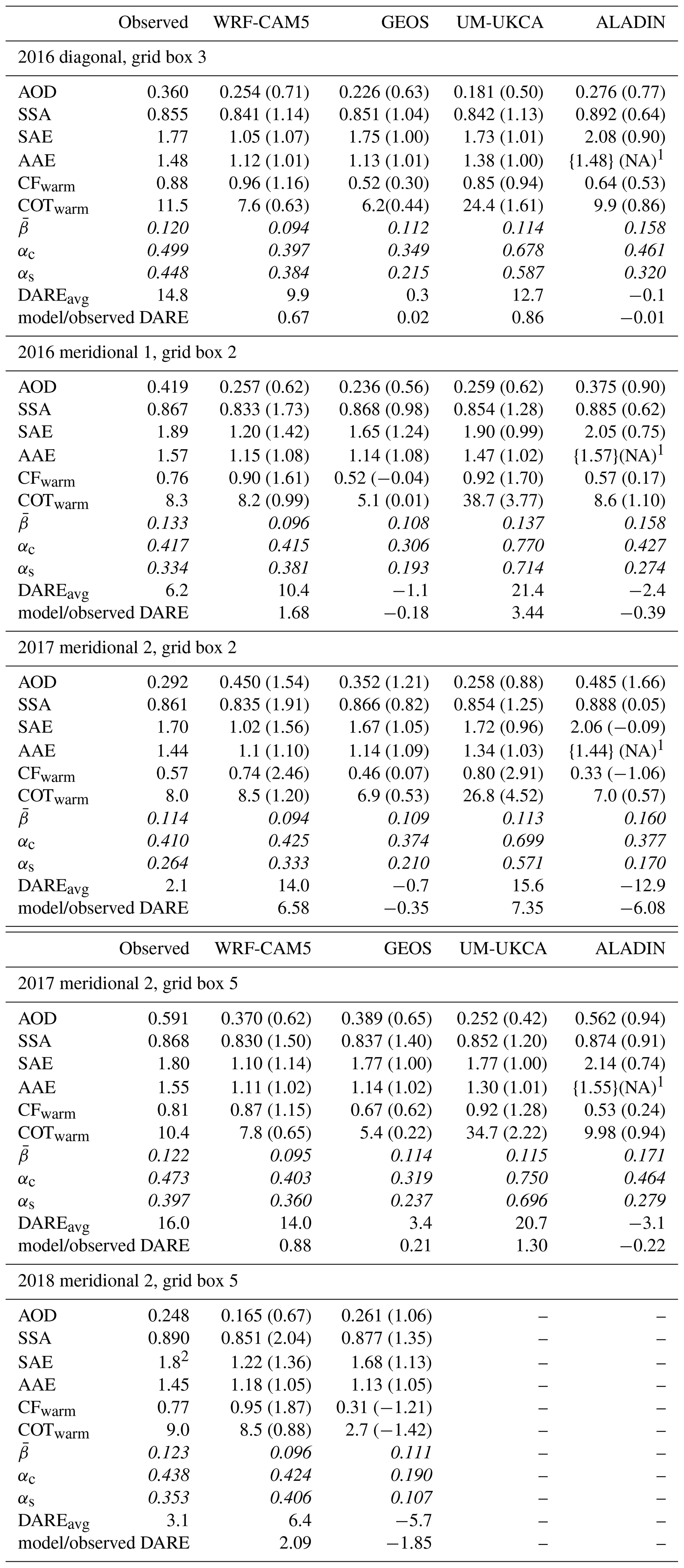
¹ AAE was not reported for the ALADIN model, so the observed value is used in the calculation of DARE. ² SAE measurements are not available for 2018, so the average value of 1.8 from 2017 is used here. Please note that “NA” stands for not available.

AAE was not reported for the ALADIN model, so the observed value is used in the calculation of DARE (Table 3). In addition, in 2018 there were problems with the measurement of SAE, so the observed value in that year is set to 1.8, since SAE in 2016 and 2017 was typically 1.7–1.9 at plume altitudes across most comparison grid boxes. Aerosol properties for the UM-UKCA model are the ambient RH values.

Equations (3) and (4) provide a valuable tool to represent the functional dependency of DARE on aerosol and cloud properties and surface albedo. However, the resulting values (Table 3) are an approximation that does not fully account for all of the factors that influence DARE. For example, a fixed solar zenith angle (30^∘) is used in calculating cloud albedo, the aerosol backscatter (rather than upscatter) fraction is used in the calculation, and this formulation does not account for the effects of Sun angle on atmospheric gaseous transmission (T_a) and on aerosol scattering; spectral variations in aerosol and radiative properties are not included either. The amount of sunlight that interacts with the aerosol at a given altitude also depends on extinction by aerosol at higher altitudes, and this is not accounted for by using a fixed atmospheric transmission factor. In addition, the calculation uses month-long grid box averages for aerosol and cloud properties. DARE does not scale linearly with SSA or the subplume albedo and, therefore, with CF_warm and COT_warm, so the mean DARE values presented here will differ from a mean of instantaneous DARE values.

To explore the limitations of Eq. (3), we perform full radiative transfer calculations for spectrally resolved upward and downward broadband fluxes (100 nm bandwidth in the visible spectrum and 500 nm beyond) for cloudy and clear skies, with and without aerosol, using libRadtran (Mayer and Kylling, 2005). From these fluxes, we calculate the instantaneous DARE in cloudy and clear skies. Finally, DARE_avg is calculated from the cloud fraction weighted DARE of both cloudy and clear skies, as in Eq. (4). To compare with the parameterized DARE_avg, the instantaneous DARE_avg are integrated over 24 h to obtain the diurnally averaged DARE. Our simulations use a mid-latitude winter gas profile and correlated k parameterization from Kato et al. (1999) for spectrally resolved results prior to spectral integration. The dark ocean in the simulation is treated as a Lambertian surface with a prescribed wavelength-dependent albedo. A slab aerosol layer is assumed for 2–5 km altitude, and the cloud layer is located at 0.7–1 km. Spectral AOD and SSA are calculated using the EAE and AAE in Table 3.

The comparison of parameterized DARE_avg with the full radiative transfer calculations are shown in Fig. S22. We find a high correlation coefficient (R²=0.95) with relatively few outliers which are mostly confined to the DARE_avg estimates for 2017 meridional 2 grid box 2. We conclude that the parameterized DARE_avg estimates in Table 3 are useful for providing a first-order estimate of how biases in key aerosol and cloud properties translate to biases in DARE in this region, and we proceed by using the parameterized DARE_avg expressions to assess the contribution of each of the variables in Table 3 to a bias in derived DARE_avg. These contributions are indicated in parentheses following the mean value of that variable; they are the ratio of DARE_avg calculated using that model's value for the given variable only and the observed values for all other variables, to DARE_avg calculated using the observed variables. For example, for the 2016 diagonal grid box 3, the WRF-CAM5 low bias in SSA alone drives a 14 % high bias in DARE_avg.

Notably, DARE_avg is positive (>0) across all five grid boxes when calculated using the observed aerosol and cloud properties and the properties from the WRF-CAM5 and UM-UKCA models. In contrast, it is negative in all five grid boxes using the properties simulated with ALADIN and negative for three of the five grid boxes for GEOS (Table 3). The modeled ambient RH 1.5–5.5 km AOD is lower than the observed low RH values for almost all grid boxes and models, but this does not translate directly to lower DARE. Even in those grid boxes where observed AOD is higher (see meridional 2 in both 2017 and 2018 in Table 3), DARE_avg calculated from the model properties can be either larger and more positive or smaller and of the opposite sign to DARE_avg calculated from the observed properties. This is because biases in different variables often counteract each other.

This can be seen in the calculations for grid box 2 in the 2017 meridional 2 transect. This example stands out in that the modeled AOD is larger than observed in three of the four models (WRF-CAM5, GEOS, and ALADIN). CF_warm in this grid box is also lower than in the other four grid boxes (0.57 versus >0.75). In the WRF-CAM5 model, this high AOD bias combines with, in particular, a high bias in modeled CF_warm, and a low bias in SSA to produce DARE_avg that is a factor of 6.6 larger than when calculated using the observed properties. In contrast, in ALADIN an AOD high bias of a similar magnitude combines with a significant low bias in CF_warm and a high bias in SSA to produce a DARE_avg that is 6.1 times larger than that using observed properties – but it is of the opposite sign.

Across the five grid boxes, biases in σ_ep (AOD) and CF_warm and COT_warm (through their role in determining α_s) alternately make the largest contributions to biases in DARE_avg in many of the models/grid boxes. Biases in SSA are usually the source of somewhat smaller DARE_avg biases, but it is a still significant contributor across most models and grid boxes. Low biases in SAE in the WRF-CAM5 and GEOS-5 models and a high bias in SAE in the ALADIN model also can drive biases of the order of 30 %–40 % through its role in determining $\overline{\mathit{\beta }}$ (see Eq. 3).

DARE_avg derived from the WRF-CAM5 properties vary from being within about 30 % of DARE_avg calculated using the observed properties in two of the five grid boxes, to having significantly high biases in the other three (factors of 1.7, 6.6, and 2.1). In these latter three cases, the consistent low bias in SSA and high bias in CF_warm more than offsets a low bias in AOD in two of the grid boxes and adds to the high bias in AOD in the third. This is not the case in 2016 diagonal grid box 3, where SSA and CF_warm are still biased low and high, respectively, but when combined with a low bias in COT_warm, the resulting DARE_avg is much close to DARE_avg from the observed properties. The excellent agreement in 2017 meridional 2 grid box 5 in DARE using the observed and WRF-CAM5 properties also results from compensating biases. The simulated AOD and COT_warm produce a low bias in DARE_avg, and the simulated SSA and (to a lesser degree) SAE and CF_warm produce a high bias in DARE_avg, nearly exactly offsetting each other. This shows how qualitatively consistent biases in a given model's representation of aerosol and cloud properties key to DARE can combine to produce a large range of biases in modeled DARE.

In GEOS, the extinction-weighted SSA in the plume introduces small (<20 %) low biases in DARE_avg in three of the grid boxes and 35 %–40 % low biases in the other two. More significant for this model is larger low biases in AOD in three of the five grid boxes and systematic low biases in CF_warm, and COT_warm. These result in values of DARE_avg that are too small and, for three of the five cases, produce negative rather than positive values. As in WRF-CAM5, biases in different variables can offset each other. For example, correcting for AOD alone would produce even larger negative values of forcing for three of the five grid boxes, increasing the difference between DARE_avg from the modeled and observed properties.

In the UM-UKCA model, a high bias in CF_warm and a large high bias in COT_warm make the subplume scene albedo of the order of a factor of 2 too high, driving large high biases in DARE_avg. This, combined with a small (∼ 0.01–0.02) low bias in SSA, more than compensates for the low bias in AOD to produce values of DARE_avg that are too large in three of the four grid boxes tested and significantly so (by factors of 3.4 and 7.4) in two of the grid boxes. Correction to just the aerosol fields would produce DARE_avg that is universally too high; correction to just the cloud fields, conversely, would produce DARE_avg that is universally too low.

The ALADIN model consistently simulates too small CF_warm and too high SSA. These are sufficient to produce a negative direct aerosol radiative effect across all five grid boxes, which is in contrast with the positive DARE_avg calculated from the observed values. In the 2017 meridional 2 grid box 2, the CF_warm bias alone is sufficient to produce negative DARE. Small low biases in AOD and COT_warm and a high bias in SAE also combine to produce values of DARE_avg that are too small (AOD and SAE) and too negative (COT_warm).

These findings support those of earlier studies (e.g., Chand et al., 2009; Stier et al., 2013; Zuidema et al., 2016) that emphasize the importance of accurately simulating cloud fraction in order to obtain accurate estimates of direct forcing by biomass burning aerosol over the SE Atlantic. They also highlight the importance of quantifying the relative roles of the aerosol and cloud properties that control the direct aerosol radiative effect, since the magnitude, sign, and source(s) of DARE biases can vary with the aerosol and cloud properties themselves. The limited analysis presented here makes it clear that models can have compensating biases, such that model improvements that make one key parameter more accurate could actually lead to less accurate simulated values of DARE. This first-order analysis provides a framework for a future study that employs full radiative transfer calculations that use, for example, the full 2D profiles of observed and modeled cloud properties and account for diurnal effects, and that accounts for uncertainties and variability in observed and modeled fields.

6 Discussion and conclusions

The WRF-CAM5 and GEOS models were used to test for representativeness of the observations of the biomass burning plume along our comparison transects, using aerosol light extinction as the metric (Sect. 4.1). This approach assumes that the models accurately represent variability in σ_ep, even if there are biases in the mean values of σ_ep. A first-order test indicates this is a good assumption in 2016, but that the two models had different levels of variability from each other and from the observations in 2017 and 2018 (Sect. 2.2). This is reflected in the different results from the two models when testing for representativeness. The representativeness of a given set of samples within the models also varies between years, even for the same transect (meridional 2), indicating systematic differences between the models at interannual timescales and/or for different locations. In addition, model invariance in the biomass burning plume aerosol intensive properties (e.g., SSA) made the models not useful for testing the representativeness of sampled aerosol intensive optical properties.

With the exception of the WRF-CAM5 model in 2018, the models simulated either comparable or higher variability σ_ep within the comparison transects. As such, with that one exception, they likely present a conservative estimate of the representativeness of the observations. Though there were some exceptions, sampled values of σ_ep in the 2–5 km altitude range across the diagonal (2016), meridional 1 (2016), and meridional 2 (2017 and 2018) transects were generally within 20 % of the approximately month-long period of each year's campaign. This altitude range encompasses the core of the biomass burning plume in most comparison grid boxes and campaign years. The fact that the modeled plume concentrations (as measured by σ_ep) at the sampled times were this close to the month-long averages is surprising given that, even with about half the ORACLES flights dedicated to routine track sampling, data were collected for, at most, only 1–2 h of the full approximately month-long campaign period in each year for a given grid box and 500 m altitude bin (Fig. 2).

Biases in the plume altitude and concentration were tested through comparisons to observed CO concentration, σ_ep, and BC and OA concentrations across 3 campaign years covering different months (September 2016, August 2017, and October 2018) and, therefore, different parts of the African biomass burning season. Biases in CO for the two models that reported it (WRF-CAM5 and GEOS) suggest underestimates in emissions or possibly in the efficiency of transport of the biomass burning plume over the SE Atlantic from the burning source regions, since CO is not affected by scavenging processes. An earlier assessment of GEOS representation of the African biomass burning plume indicates that, for that model, transport biases are the more likely cause (Das et al., 2017). In both models, the low bias in CO was larger in October 2018, which is towards the end of the biomass burning season, than in August 2017 and September 2016. Notably, both of these models use QFED2 emissions.

In the core of the plume, low biases in BC in WRF-CAM5 and GEOS were somewhat smaller than the CO low biases. In other words, the CO:BC ratio was somewhat lower in the models than the observations, particularly in the October 2018 meridional 2 transect and more so in the GEOS model than in WRF-CAM5. The ratio of CO:BC in biomass burning primary emissions depends on the material being burned and the efficiency of burning (smoldering versus flaming; e.g., Reid et al., 2005), but this is set within the QFED emissions and so cannot explain these intermodel differences. Differences in anthropogenic sources could also be contributing (e.g., WRF-CAM5 uses EDGAR-HTAP while GEOS uses AeroCom Phase II), as could differences in the background CO concentrations. In October 2018, when differences between the models and the observations were largest, the biomass burning plume was less intense, so for that month the background and anthropogenic emissions could be more strongly influencing the CO and BC concentrations. For the biomass burning aerosol itself, given the common emissions dataset used by the two models, differences in the CO:BC ratio between the models must be due to differences in the in-atmosphere chemistry and processing, combined with dynamics, leading to different aerosol scavenging rates. Notably, WRF-CAM5 has more sophisticated aerosol chemistry than GEOS. Greater scavenging losses in reality than in the models in the first couple of days after emission, e.g., mostly over the land, could also be contributing to the lower CO:BC ratio in models than in the observations.

Model biases in BC versus in OA, and how these biases evolve along the aerosol transport pathway, also give some insight to model processes. This is because BC is a refractory, primary aerosol; it is not produced or destroyed in the atmosphere (Bond et al., 2013). OA, on the other hand, is emitted directly as an aerosol, is being formed in the atmosphere in secondary production from gas phase constituents, and is lost in the atmosphere through evaporation back to the gas phase, photo-chemical transformation, and/or heterogenous oxidation (e.g., Hallquist et al., 2009; O'Brien and Kroll, 2019).

In most grid boxes above the boundary layer, there is a smaller low bias (or in some locations a greater high bias) in OA than in BC, in the three models that report both parameters (WRF-CAM5, GEOS, and UM-UKCA). The higher OA:BC ratio in the models, as reflected in their respective relative biases, is more pronounced in 2017 and 2018 and in the GEOS model, and it tends to be lower at the core of the plume than at the plume edges. This could originate from a number of model biases, including primary emissions having too high a ratio of OA:BC, too much secondary organic aerosol (SOA) production, and/or insufficient loss of organics with aerosol aging. Again, WRF-CAM5 and GEOS both use the GFED emissions, so they should have the same OA:BC ratio in primary emissions. The UM-UKCA model, however, uses the FEER inventory, which may have a different OA:BC ratio in emissions from these fires. For OA, the in-atmosphere production and losses can be significant. Previous studies have shown that SOA can be produced rapidly – within minutes to hours – after emission (e.g., Jimenez et al., 2009; Bond et al., 2013). OA can also be produced and lost on timescales of days to >1 week after emission (Capes et al., 2008; Wagstrom et al., 2009; Cubison et al., 2011; Jolleys et al., 2015; Hodzic et al., 2015; Collier et al., 2016; Konovalov et al., 2019; Hodshire et al., 2019; Cappa et al., 2020).

Model-based age estimates indicate that the aerosol we sampled during ORACLES was almost always at least 2 d old, so our observations only inform us how the OA:BC ratio evolved starting several days after emission. Observations from ORACLES may ultimately not be able to discriminate the loss of OA through aging from differences in the OA mass in the source emissions. Regardless, processes that drive the in-atmosphere OA losses on these longer (multi-day) timescales are not implemented in any of the models included here, and this could lead to higher model OA:BC ratios for aged aerosol. However, we cannot rule out too high a ratio of OA:BC in emissions and too much secondary organic aerosol (SOA) production, although the latter is less likely as models tend to show low production of SOA compared to observations (Hodzic et al., 2016).

Biases in σ_ep stem from the combined biases in the aerosol component (e.g., BC and OA) masses and in the mass extinction efficiency. The latter depends in part on aerosol water content, especially above ∼ 40 %–50 % RH. Here, the in situ observed values of σ_ep were made at low (<40 %) RH, whereas the HSRL-2 measured and modeled values were at ambient RH. All four models significantly underestimate σ_ep, with low biases in σ_ep greater than for BC or OA. Consistent with this, Shinozuka et al. (2020) calculated a proxy for the mass extinction efficiency, ${\mathit{\sigma }}_{\mathrm{ep}}/$(OA+BC), from the observations and models, and found it was lower in the models than the observations, including for the 3–6 km altitude column. For spherical particles and mid-visible wavelengths, the mass scattering efficiency increases with aerosol diameter between about 100 and 450 nm diameter, then decreases above about 600 nm (e.g., Saide et al., 2020). The SAE provides a proxy for aerosol size; assuming a monomodal size distribution, typical SAE values indicate an aerosol effective diameter of approximately 380–400 nm for ALADIN (SAE of 2.0–2.2), 420 nm for the observations and GEOS (SAE of 1.8), 400–420 nm for UM-UKCA (SAE of 1.8–2.0), and 700 nm for WRF-CAM5 (SAE of 1.0) (Schuster et al., 2006). Because the mass extinction efficiency peaks at about 500 nm, aerosol size alone would drive it higher for the observations, GEOS, and UM-UKCA models than for ALADIN – but it should be comparable for the observations and WRF-CAM5 despite the SAE differences (see Fig. 10a of Saide et al., 2020). In this case, a more likely source of the apparent low bias in model mass extinction efficiency are the real indices of refraction used in the models for aerosol components, as the OA real refractive index used in WRF-CAM5 is 1.45, while the literature values for biomass burning are more often in the 1.52–1.55 range (Aldhaif et al., 2018).

The CO, BC, OA, and σ_ep comparisons all indicate that the models simulated plumes that are too vertically diffuse. Too much vertical diffusion in the models maybe responsible for, in particular, the plume top terminating at lower altitude in the in situ observations than in some of the simulations, often leading to low biases in modeled CO, BC, OA, and σ_ep in the 2–5 km altitude range and significant relative (but small absolute) high biases in the 5–6 km range in the comparisons. It is not fully clear, however, whether this is a robust result, given that the HSRL-2, like the models, measured extinction extending to higher altitudes than the in situ observations did (Sect. 4.2.3).

In the GEOS, UM-UKCA, and ALADIN models, it also appears that either the smoke is not lofted sufficiently high over the continent or that the subsidence is too strong in the models, particularly in 2016 but also in 2018 (for GEOS). In the WRF-CAM5 model, all biomass burning emissions are injected into the surface model layer; this smoke is lifted and mixes in the continental boundary layer, which grows to a depth of typically about 3.5–4.0 km (Labonne et al., 2007) but can reach 4.5–5.5 km (Ryoo et al., 2021). In the UM-UKCA model, emissions are added to the boundary layer such that concentrations taper from higher values at the surface to zero at 3 km above the surface. Burning progresses southward through the biomass burning season, with the land surface elevation where burning is occurring shifting from <500 m in the Congo Basin to >1500 m in the Namibian Kalahari dryland. This increase in elevation assists the lofting of the smoke (Ryoo et al., 2021). Notably, the models underestimate the smoke plume height during the later months of the burning season when fires are sourced at higher elevations, indicating possible issues with the model representation of boundary layer development over land. It is also possible that lifting of the plume driven by subgrid scale processes (Freitas et al., 2006) and/or by aerosol self-lifting through absorption and heating (Boers et al., 2010; de Laat et al., 2012) that is not fully accounted for in the models.

The tendency for the models to have too diffuse a bottom edge of the plume and a plume that is too low in altitude will lead to greater mixing of the aerosol into clouds and, therefore, aerosol–cloud interactions. The vertical distance between the cloud top and the biomass burning plume could also affect the semi-direct forcing in this region (Adebiyi and Zuidema, 2018). Based on the altitude dependence of the model bias in aerosol concentrations, the impact of these biases is more pronounced in September 2016 and August 2017 than in October 2018.

While the magnitude of aerosol scattering and absorption over this region is largely controlled by above-cloud AOD, or vertically integrated σ_ep, the sign of the direct effect is controlled by the aerosol SSA in the plume and by subplume albedo (here, largely controlled by CF_warm). In the observations, SSA increases with altitude in the plume in September 2016 and October 2018 but not in August 2017. These vertical variations were not captured by any of the models (Fig. 14). Both WRF-CAM5 and GEOS do, however, have overall higher SSA in August (2018) than in September and October (2016 and 2018), as do the observations.

Co-albedo (1-SSA) differences, weighted by σ_ep, translate directly to differences in absorbed energy. Ambient RH SSA is lower (and co-albedo higher) than the observed dry SSA in the WRF-CAM5, GEOS, and UM-UKCA models; in ALADIN, the SSA is both higher and more variable than observed. These biases vary with altitude, with some of the largest differences in modeled and observed SSA towards the top of the plume. Large SSA biases at altitudes with very little light extinction will, however, have little impact on DARE. At altitudes where the plume is largely concentrated (2.5–5 km), on average, the co-albedo in the model is biased high by ∼ 5 %–10 % in UM-UKCA, ∼15 % in GEOS-5, and 15 %–20 % in WRF-CAM5, relative to the dry observed values. ALADIN co-albedo is biased low by about 10 %–35 % on average. These biases combine with biases in σ_ep to affect the atmospheric absorption and, therefore, in addition to DARE, the marine low cloud responses to atmospheric absorption above the clouds.

All of the values above are for mid-visible (530 or 550 nm) SSA, but of course DARE operates over the full solar spectrum. Spectral SSA is, in turn, directly related to SAE and AAE. Thus, uncertainty in AAE translates into uncertainty in spectral SSA and, in the context of DARE, the amount of sunlight absorbed in the atmosphere. The observed values of σ_ap are well constrained at 530 nm, but they are very uncertain at shorter and longer wavelengths (470 and 660 nm) where the PSAP measurements have not been as robustly calibrated. For the ORACLES biomass aerosol, the two different Virkkula (2010) calibrations yield AAE values of about 1.2 (wavelength-averaged correction) and 1.5 (wavelength-specific correction), whereas the modeled values average 1.1–1.2, with little difference across the 3 field campaign years. Notably, the lower values agree well with AAE values measured near Ascension Island during the UK CLARIFY 2017 campaign, which used a photoacoustic spectrometer to measure absorption (Taylor et al., 2020).

A question is whether this uncertainty in AAE leads to a significant uncertainty in DARE. By definition, the AAE parameterization of absorption change versus wavelength is linear in the log space, so, for higher AAE, the increase in absorption at shorter wavelengths is stronger than the decrease towards longer wavelengths. However, the downwelling solar spectrum in the troposphere peaks at ∼ 450 nm and drops off more rapidly at shorter wavelengths than longer wavelengths. The impact on atmospheric absorption, and therefore DARE, of differing values of AAE results from the convolution of these spectral dependencies of aerosol absorption and the downwelling solar radiation.

To quantify this effect, we calculated the 300–750 nm integrated atmospheric absorption for aerosol with AAE of 1.0, 1.2, and 1.5, using a fixed 550 nm SSA of 0.86, a value of SAE equal to 1.8, and a clear-sky spectral downwelling solar radiation typical of mid-latitude fall. We find that integrated absorption for AAE equal to 1.5 is only 3 % greater than for AAE equal to 1.2 and only 4 % greater than for AAE equal to 1.0. The offsetting effects of the spectral dependencies of AAE and solar flux allow DARE to be fairly insensitive to uncertainties in AAE. Therefore, the observed model biases in AAE – relative to either of the possible observed AAE values – will not contribute significantly to biases in modeled DARE, consistent with the findings of de Graaf et al. (2014).

In the ORACLES study region, the subplume albedo is a function of CF_warm, cloud albedo (α_c), and the ocean surface albedo. Because of the large difference between the cloud albedo and ocean surface albedo, CF_warm is a strong controller of the subplume albedo, with higher CF_warm driving more positive DARE. Across our comparison transects, WRF-CAM5 tended to overestimate CF_warm and GEOS and ALADIN tended to underestimate CF_warm, with the UM-UKCA coming closest to reproducing the observations but still tending to be biased high (Fig. 18). GEOS and ALADIN, in particular, also had different gradients in CF_warm with latitude (meridional transects) and longitude (zonal transect) than was observed; the 2016 diagonal transect is the only comparison transect where all models largely captured the CF_warm gradient. The large difference in COT_warm between the observations, WRF-CAM5, GEOS, and ALADIN (range of 8–11) versus in UM-UKCA (range of 24–39) translates to a significantly high bias in α_c in the UM-UKCA model, ranging from 40 % (2016 diagonal grid box 3) to 85 % (2016 meridional grid box 2; Sect. 5 and Table 3). This will combine with any high biases in CF_warm in the UM-UKCA model to produce direct aerosol radiative effects that are too positive (warming) and is sufficient to more than compensate for any small low biases in CF_warm.

First-order calculations of DARE for select grid boxes in the comparison transects demonstrate how these translate into biases in aerosol radiative effects for the above-cloud aerosol (Sect. 5). Earlier studies have shown that different models simulate everything from large negative to large positive direct aerosol radiative forcing by the biomass burning aerosol over the SE Atlantic (Zuidema et al., 2016 and Stier et al., 2013). Consistent with this, DARE calculated using simulated aerosol and cloud properties for five of our comparison grid boxes spanned −12 to 20 Wm⁻² across the four models. In contrast, DARE calculated from the observed properties were all positive, ranging from 2 to 16 Wm⁻². Using this simplified calculation, we showed that, across these five grid boxes, biases in σ_ep (and therefore AOD) and in CF_warm and COT_warm (through their role in determining the albedo below the aerosol plume) alternately make the largest contributions to biases in DARE in many of the models/grid boxes. SSA is a source of smaller but still significant biases in some cases, as is, in one case, the simulated SAE through its impact on the aerosol hemispheric backscatter fraction.

Calculations of how DARE is affected by biases in each of the observed aerosol and cloud properties included in this comparison study reveal that biases in different properties often produce offsetting biases in DARE. As a result, improving the model representation of just one field (e.g., AOD for GEOS or just the cloud fields for UM-UKCA) would actually increase the bias in simulated DARE. This highlights the importance of testing for and correcting biases in all simulated properties that affect DARE, which in this region includes the representation of low marine clouds. It also provides motivation for a more thorough assessment of direct aerosol radiative forcing over the SE Atlantic that accounts for the model biases identified herein.