Ice multiplication from ice–ice collisions in the high Arctic: sensitivity to ice habit, rimed fraction, ice type and uncertainties in the numerical description of the process

Atmospheric models often fail to correctly reproduce the microphysical structure of Arctic mixed-phase clouds and underpredict ice water content even when the simulations are constrained by observed levels of ice nucleating particles. In this study we investigate whether ice multiplication from breakup upon ice–ice collisions, a process missing in most models, can account for the observed cloud ice in a stratocumulus cloud observed during the Arctic Summer Cloud Ocean Study (ASCOS) campaign. Our results indicate that the efficiency of this process in these conditions is weak; increases in fragment generation are compensated for by subsequent enhancement of precipitation and subcloud sublimation. Activation of collisional breakup improves the representation of cloud ice content, but cloud liquid remains overestimated. In most sensitivity simulations, variations in ice habit and prescribed rimed fraction have little effect on the results. A few simulations result in explosive multiplication and cloud dissipation; however, in most setups, the overall multiplication effects become substantially weaker if the precipitation sink is enhanced through cloud-ice-to-snow autoconversion. The largest uncertainty stems from the correction factor for ice enhancement due to sublimation included in the breakup parameterization; excluding this correction results in rapid glaciation, especially in simulations with plates. Our results indicate that the lack of a detailed treatment of ice habit and rimed fraction in most bulk microphysics schemes is not detrimental for the description of the collisional breakup process in the examined conditions as long as cloud-ice-to-snow autoconversion is considered.

1 Introduction

Cloud feedbacks play an important role in Arctic climate change (Cronin and Tziperman, 2015; Kay et al., 2016; Tan and Storelvmo, 2019) and sea-ice formation (Burt et al., 2015; Cao et al., 2017). However, despite their significant climatic impact, Arctic mixed-phase clouds remain a great source of uncertainty in climate models (Stocker et al., 2013; Taylor et al., 2019). To accurately predict the radiative effects of mixed-phase clouds in models, an adequate description of their microphysical structure, such as the amount and distribution of both liquid water and ice, is required (Korolev et al., 2017). Both ice nucleation and liquid drop formation require seed particles to be present which are known as ice nucleating particles (INPs) and cloud condensation nuclei (CCN), respectively. However, the observed ice crystal number concentrations (ICNCs) are often much higher than the observed INP concentrations in the Arctic (Fridlind et al., 2007, 2012; Gayet et al., 2009; Lloyd et al., 2015), where INPs are generally sparse (Wex et al., 2019). Moreover, model simulations constrained by INP measurements frequently underpredict the observed amount of ice (Fridlind and Ackerman, 2019).

Secondary ice processes (SIPs) have been suggested as the reason why ice crystal concentrations exceed INP levels (Field et al., 2017; Fridlind and Ackerman, 2019). SIPs involve the production of new ice crystals in the presence of pre-existing ice without requiring the presence of an INP. The most well-known mechanism is rime splintering (Hallet and Mossop, 1974), which refers to the ejection of ice splinters when ice particles collide with supercooled liquid drops. Rime splintering is active only in a limited temperature range, between −8 and −3 ^∘C, and requires the presence of liquid droplets both smaller than 13 µm and larger than 25 µm (Hallett and Mossop, 1974; Choularton et al., 1980). Moreover, recent studies have shown that rime splintering alone cannot explain the observed ICNCs in polar clouds even within the optimal temperature range (Young et al., 2019; Sotiropoulou et al., 2020, 2021). Ice fragments may also be generated when a relatively large drop freezes and shatters (Lauber et al., 2018; Phillips et al., 2018); drop shattering, however, has been found to be insignificant in polar conditions (Fu et al., 2019; Sotiropoulou et al., 2020). Finally, ice multiplication can occur from mechanical breakup due to ice–ice collisions (Vardiman et al., 1978; Takahashi et al., 1995). This process has been also identified in in situ measurements of Arctic clouds (Rangno and Hobbs, 2001; Schwarzenboeck et al., 2009).

Schwarzenboeck et al. (2009) found evidence of crystal fragmentation in 55 % of in situ observations of ice particles collected with a cloud particle imager during the ASTAR (Arctic Study of Aerosols, Clouds and Radiation) campaign. However, natural fragmentation could only be confirmed for 18 % of these cases, which was identified by either subsequent growth near the break area or/and a lack of a fresh breakup line (which indicates shattering on the probe). For the rest of their samples, artificial fragmentation could not be excluded. Moreover, their analysis included only crystals with stellar shape and sizes around 300 µm or roughly larger. This suggests that the frequency of collisional breakup in Arctic clouds is likely higher in reality compared to what is indicated in their study. Yet, despite the potential impact of this process in Arctic conditions, it has received little attention from the modeling community.

Fridlind et al. (2007) and Fu et al. (2019) investigated the contribution from ice–ice collisions in an autumnal cloud case observed during the Mixed-Phase Arctic Cloud Experiment (M-PACE) and found that the process could not account for the observed ice content at in-cloud temperatures between −8.5 and −15.5 ^∘C. The parameterization of the breakup process used in these studies was based on the laboratory data of Vardiman (1978). However, there are significant shortcomings in the available laboratory measurements. For example, in Vardiman (1978) the ice particles were collected in a mountainside below cloud base, and thus the collected samples were impacted by sublimation. Takahashi et al. (1995) also used an unrealistic setup: they performed collisions between centimeter-size hail balls, while one of the colliding hydrometeors was unrimed and fixed. These considerations preclude deriving an accurate parameterization for ice multiplication due to collisional breakup from this data alone.

Phillips et al. (2017a, b) developed a more advanced treatment of ice multiplication from ice–ice collisions, which is based on the above-mentioned laboratory results but further considers the impact of collisional kinetic energy, ice habit, ice type and rimed fraction. More specifically, their parameterization accounts for dendritic and non-dendritic planar ice shapes; the latter includes plates, columns and needles, thus all the ice habits for which there are no available observations of breakup. Moreover, to correct the effect of sublimation in the data of Vardiman (1978), they adjusted the fragile coefficient (term ψ in Appendix A) in their description. While these approximations are a source of uncertainty, their parameterization has been tested in polar clouds (Sotiropoulou et al., 2020, 2021) and resulted in ice enhancements that could explain the observed ICNCs. Sotiropoulou et al. (2020, 2021) focused on relatively warm polar clouds (−3 to −8 ^∘C), for which rime splintering is considered to be the dominant SIP mechanism; yet the efficiency of this process alone was found to be limited in these studies. In Sotiropoulou et al. (2020) the combination of both rime splintering and collisional breakup was essential to explain observed ICNCs, while in Sotiropoulou et al. (2021) rime splintering had hardly any impact. Zhao et al. (2021), however, found limited efficiency of this process in Arctic clouds with cloud-top temperatures between −10 and −15 ^∘C, while other formation processes (heterogeneous freezing and drop shattering) appeared to be more important.

In this study, we aim to investigate the role of ice–ice collisions in high-Arctic clouds with cloud-top temperatures of −9.5 to −12.5 ^∘C, a temperature range for which previous studies found limited efficiency in the process (Fridlind et al., 2007; Fu et al., 2019; Zhao et al., 2021). The Phillips parameterization is implemented in the MIT-MISU Cloud and Aerosol (MIMICA) large eddy simulation (LES) model to examine its performance for a stratocumulus case observed during the Arctic Summer Cloud Ocean Study (ASCOS) campaign in the high Arctic. To identify the optimal microphysical conditions for ice multiplication through collisional breakup, the sensitivity of the results to the assumed rimed fraction, ice habit and ice type (e.g., cloud ice or snow) of the colliding ice particles is examined.

2 Field observations

The ASCOS campaign was deployed on the Swedish icebreaker Oden between 2 August and 9 September 2008 in the Arctic Ocean, to improve our understanding of the formation and life-cycle of Arctic clouds. It included an extensive suite of in situ and remote sensing instruments, a description of which can be found in Tjernström et al. (2014). Here we only offer a brief description of the instruments and measurements utilized in the present study.

2.1 Instrumentation

Information on the vertical atmospheric structure was derived from Vaisala radiosondes released every 6 h with 0.15 ^∘C and 3 % uncertainty in temperature and relative humidity profiles, respectively. Cloud boundaries were derived from a vertically pointing 35 GHz Doppler millimeter cloud radar (MMCR; Moran et al., 1998) with a vertical resolution of 45 m and two laser ceilometers. CCN concentrations were measured by an in situ CCN counter (Roberts and Nenes, 2005), set at a constant supersaturation of 0.2 % (with an uncertainty of ±0.04 %; Moore et al., 2011) based on typical values used in other similar expeditions (Bigg and Leck, 2001; Leck et al., 2002). The total uncertainty in CCN concentration derived from counting statistics and fluctuations in pressure and flow rate is 7 %–16 % for CCN concentrations above 100 cm⁻³ (Moore et al., 2011). Vertically integrated liquid water path (LWP) was retrieved from a dual-channel microwave radiometer with an uncertainty of 25 g m⁻² (Westwater et al., 2001). Ice water content (IWC) was estimated from the radar reflectivity observed by the MMCR using a power-law relationship (e.g., Shupe et al., 2005) with a factor of 2 uncertainty. The ice water path (IWP) was integrated from the IWC estimates.

2.2 ASCOS case study

A detailed description of the conditions encountered during the ASCOS campaign is available in Tjernström et al. (2012). Our focus here is on a stratocumulus deck observed between 30 and 31 August when Oden was drifting with a 3 km×6 km ice floe at approximately 87^∘ N. During that time, relatively quiescent large-scale conditions prevailed, characterized by a high-pressure system and large-scale subsidence in the free troposphere and only weak frontal passages (Tjernström et al., 2012).

Our simulations are initialized with thermodynamic and cloud liquid profiles representing conditions observed on 31 August at 06:00 UTC (Fig. 1). These profiles display a cloud layer between 550 and 900 m above ground level (a.g.l.) at temperatures between −7 and −10 ^∘C capped by a temperature and humidity inversion of about 5 ^∘C and 0.5 g kg⁻¹, respectively. A weak secondary temperature inversion is also observed at about 370 m a.g.l., indicating that the cloud is decoupled from the surface; this type of vertical structure, with a decoupled surface and cloud layer, dominated during the whole ASCOS experiment (Sotiropoulou et al., 2014). More generally, this case study is representative of typical cloudy boundary layers over sea ice, where co-existing temperature and humidity inversions are frequently observed (Sedlar et al., 2012) and clouds are often decoupled from any surface sources of, for example, moisture (Sotiropoulou et al., 2014).

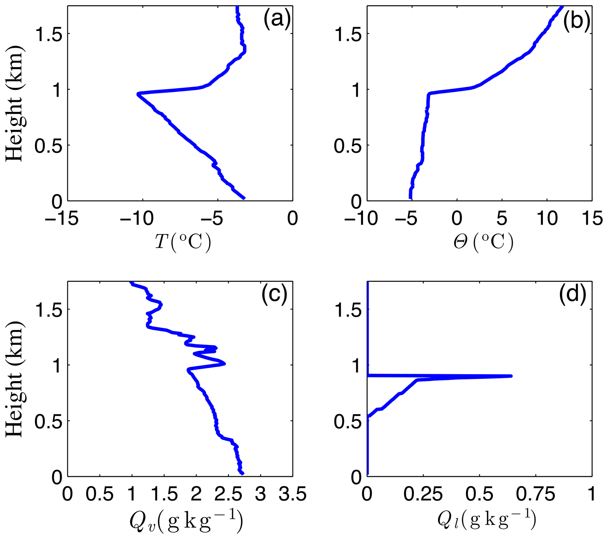
Figure 1 Radiosonde profiles of (a) temperature (T), (b) potential temperature (Θ) and (c) specific humidity (Q_v) used to initialize the LES. The profile of cloud liquid (Q_l) in (d) is integrated from radiometer measurements.

The observed cloud layer remained “stable” for about 12 h prior to the selected profile and began dissipating after 31 August at 09:00 UTC. A substantial reduction in the background aerosol concentration has been suggested as a possible cause for the sudden collapse of the cloud layer, which cannot be simulated by models without prognostic aerosol processes (Stevens et al., 2018). For this reason, we will use observational statistics from the period with the persistent stratocumulus conditions to evaluate our results, although simulations are allowed to run for 24 h in a quasi-equilibrium state.

3 Model and methods

3.1 LES setup

The MIMICA LES (Savre et al., 2014) solves a set of non-hydrostatic prognostic equations for the conservation of momentum, ice–liquid potential temperature and total water mixing ratio with an anelastic approximation. A fourth-order central finite-difference formulation determines momentum advection, and a second-order flux-limited version of the Lax–Wendroff scheme (Durran, 2010) is employed for scalar advection. Equations are integrated forward in time using a second-order leapfrog method and a modified Asselin filter (Williams, 2010). Subgrid-scale turbulence is parameterized using the Smagorinsky–Lilly eddy-diffusivity closure (Lilly, 1992), and surface fluxes are calculated according to Monin–Obukhov similarity theory.

MIMICA employs a bulk microphysics scheme with a two-moment approach for cloud droplets, rain and cloud ice, graupel, and snow particles. Mass mixing ratios and number concentrations are treated prognostically for these five hydrometeor classes, whereas their size distributions are defined by generalized Gamma functions. Cloud droplet and raindrop processes follow Seifert and Beheng (2001), while liquid–ice interactions are parameterized as in Wang and Chang (1993). Collisions between cloud ice larger than 150 µm and droplets larger than 15 µm, or raindrops, result in graupel formation; the efficiency of this conversion increases with increasing ice particle size. Graupel is also formed when snow and liquid particle collisions occur. These liquid particles can also be directly collected by graupel. Self-aggregation of cloud ice particles results in snow; this is the only snow formation mechanism in the default microphysics scheme. Self-aggregation is also allowed between snow particles, droplets larger than 15 µm and rain; aggregated snow particles and droplets are converted to graupel and raindrops, respectively. A simple parameterization for CCN activation is applied (Khvorostyanov and Curry, 2006), in which the number of cloud droplets formed is a function of the modeled supersaturation and a prescribed background aerosol concentration. A detailed radiation solver (Fu and Liou, 1992) is coupled to MIMICA to account for cloud radiative properties when calculating the radiative fluxes.

The model configuration adopted is based on Ickes et al. (2021), who simulated the same case to examine the performance of various primary ice nucleation schemes. All simulations are performed on a $\mathrm{96}\times \mathrm{96}\times \mathrm{128}$ grid with constant horizontal spacing $\mathrm{d}x=\mathrm{d}y=\mathrm{62.5}$ m. The simulated domain is 6 km×6 km horizontally and 1.7 km vertically. At the surface and in the cloud layer the vertical grid spacing is 7.5 m, while between the surface and the cloud base it changes sinusoidally, reaching a maximum spacing of 25 m. The integration time step is variable (∼ 1–3 s), calculated continuously to satisfy the Courant–Friedrichs–Lewy criterion for the leapfrog method. While this approach prevents numerical instabilities, its dynamic nature does not allow sensitivity simulations to be performed with exactly the same time step. Lateral boundary conditions are periodic, while a sponge layer in the top 400 m of the domain dampens vertically propagating gravity waves generated during the simulations. To accelerate the development of turbulent motions, the initial ice–liquid potential temperature profiles are randomly perturbed in the first 20 vertical grid levels with an amplitude less than $\mathrm{3}\times {\mathrm{10}}^{-\mathrm{4}}$ K.

Surface pressure and temperature are set to 1026.3 hPa and −3.2 ^∘C, respectively, constrained by surface sensors deployed on the ice pack. The surface moisture is set to the saturation value which reflects summer ice conditions. The surface albedo is assumed to be 0.85, which is representative of a multi-year ice pack. In MIMICA, subsidence is treated as a linear function of height: $w_{\mathrm{LS}}=-D_{\mathrm{LS}}\cdot z$, where D_LS is set to $\mathrm{1.5}\times {\mathrm{10}}^{-\mathrm{6}}$s ⁻¹ and z is the height in meters. Finally, the prescribed number of CCN is set to 30 cm⁻³ over the whole domain, which represents mean accumulation mode aerosol concentrations observed during the stratocumulus period (Igel et al., 2017). The duration of all simulations is 24 h, in which the first 4 h constitute the spin-up period.

3.2 Ice formation processes in MIMICA

3.2.1 Primary ice production

Ickes et al. (2021) recently implemented several primary ice production (PIP) schemes in MIMICA. Here, we utilize the empirical ice nucleation active site density parameterization for immersion freezing, which is based on Connolly et al. (2009) and was further developed by Niemand et al. (2012) for Saharan dust particles. This formulation was used by Ickes et al. (2017) to describe the freezing behavior of different dust particle types, including microline (Appendix A). Microcline is a feldspar type that is known to be an efficient INP (Atkison et al., 2013). As no aerosol composition (or INP) measurements are available for the ASCOS campaign, we will use this INP type as a proxy for an aerosol constituent that can produce primary ice at the relatively warm sub-zero temperatures (−7 to −10 ^∘C) of the initial observed cloud profile (Fig. 1a). At these temperatures it is reasonable to assume that most of the PIP occurs through immersion freezing (Andronache, 2017), i.e., that an aerosol must be both CCN active and contain ice-nucleating material to initiate ice production. Thus, we will simply assume that a specified fraction of the CCN population contains some efficient ice-nucleating material, here represented as feldspar, and match this fraction so that the model simulates reasonable values of LWP, IWP and ICNC (Appendix A; Sect. S1 in the Supplement). Based on this procedure, we infer that the CCN population contains 5 % microline, a value that results in realistic primary ICNCs (Wex et al., 2019) but in an underestimate of the IWP and an overestimate of the LWP (Sect. S1, Fig. S1). Note that even though we assume this relatively high fraction of ice-nucleating material (Sect. S1, Fig. S1), MIMICA still underestimates the IWP; we postulate that omitting the effects of secondary ice production may be the reason for this bias.

3.2.2 Ice multiplication from ice–ice collisions

The observed in-cloud temperatures are generally below the rime splintering temperature range except for the somewhat warmer temperatures near cloud base (Fig. 1a). Some studies indicate that drop shattering is ineffective in Arctic conditions (Fu et al., 2019; Sotiropoulou et al., 2020), while Zhao et al. (2021) have found a significant contribution from this process. Nevertheless, our simulations suggest inefficiency of both these mechanisms in the examined conditions as the concentration of large raindrops is too low (below 0.1 cm⁻³) to initiate them (Fig. S1c). Hence we focus solely on ice multiplication from ice–ice collisions.

We implement the parameterization developed by Phillips et al. (2017a) in MIMICA and allow for ice multiplication from cloud-ice–cloud-ice, cloud-ice–graupel, cloud-ice–snow, snow–graupel, snow–snow and graupel–graupel collisions (Appendix B). The generated fragments are considered “small ice” crystals and are added to the cloud ice category in the model. The Phillips parameterization explicitly considers the effect of ice type, ice habit and rimed fractions of the colliding particles on fragment generation (Appendix B). The sensitivity of the model performance to these parameters is examined through sensitivity simulations. Additional tests are also performed to quantify the sensitivity to other sources of uncertainty, such as the applied correction for the sublimation effects in the data of Vardiman (1978) (see Sect. 1) and the estimated number of fragments.

3.3 Sensitivity simulations

A detailed description of the sensitivity tests is provided in this section, while a summary is offered in Table 2.

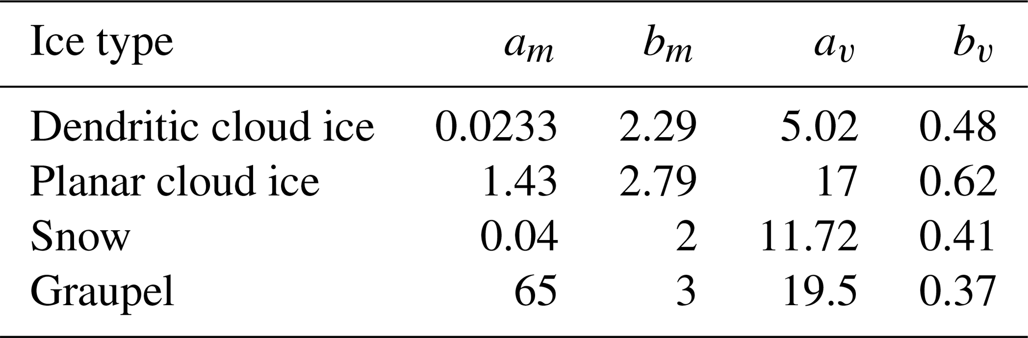
Table 1 Characteristic parameters in the mass–diameter ($m=a_m{D}^{b_m}$) and fall-speed–diameter ($v=a_v{D}^{b_v}$) relationships (see Sect. 3.3.1).

Table 2 List of sensitivity simulations (see Sect. 3.3).

3.3.1 The role of ice habit

Cloud ice observed within the examined temperature range can either be shaped as a dendrite or a plate depending on the supersaturation with respect to ice (Pruppacher and Klett, 1997). However, as the mean vapor density excess in the simulated cloud layer varies between 0.03 and 0.22 g m⁻³, it is not clear which shape should theoretically dominate (Pruppacher and Klett, 1997). Moreover, observations often indicate variable shapes within the same temperature conditions (Mioche et al., 2017). The formulation for ice multiplication due to breakup is substantially different for these two ice habits, with plates being included in the non-dendritic planar ice category (Appendix B).

MIMICA allows for variable treatment of the ice habit for the cloud ice category. These variations correspond to different characteristic parameters in the mass–diameter ($m=a_m{D}^{b_m}$) and fall-speed–diameter ($v=a_v{D}^{b_v}$) relationships (Table 1). To test the sensitivity of our results to the assumed cloud ice habit, the two simulations CNTRLDEN and CNTRLPLA are performed. “CNTRL” refers to simulations that account only for PIP, while the suffixes “DEN” and “PLA” indicate dendritic and non-dendritic planar cloud ice shape, respectively. Note that particle properties in CNTRLPLA simulations are adapted for plates (Pruppacher and Klett, 1997), while the non-dendritic planar category in the Phillips parameterization encompasses a larger range of shapes (columns, needles, etc.).

Characteristic parameters for graupel in the default MIMICA version are relatively large, with a_v being 1 order of magnitude larger than the values adapted in other stratocumulus schemes (e.g., Morrison et al., 2005). This difference has a weak impact on simulations that do not account for collisional breakup. However, if breakup is active, fragment generation is a function of collisional kinetic energy, and the results become more sensitive to the choice of these parameters. Since Arctic clouds are characterized by weak convective motions and the formation of large rimed particles is not favored, the characteristic parameters of graupel are adjusted following Morrison et al. (2005) (Table 1).

3.3.2 The role of rimed fraction

F_BR is parameterized as a function of the rimed fraction (Ψ) of the ice crystal or snowflake that undergoes breakup; fragment generation from breakup of graupel does not depend on Ψ (see Appendix B). This parameter is not explicitly predicted in most bulk microphysics schemes but can substantially affect the multiplication efficiency of the breakup process (Sotiropoulou et al., 2020). For this reason, we will consider values of Ψ for cloud ice and snow between 0.1 (lightly rimed) and 0.4 (heavily rimed) (Phillips et al., 2017a, b); graupel particles are considered to have Ψ≥0.5. Both Sotiropoulou et al. (2020) and (2021) found that ice multiplication in polar clouds at temperatures above −8 ^∘C is initiated only when a highly rimed fraction of cloud ice and snow is assumed. Their conclusions, however, may not be valid for our case as the temperature and microphysical conditions are substantially different.

The effect of varying Ψ is examined for the two ice habits that prevail in the observed temperature range (Sect. 3.2.2). The performed simulations are referred to as BRDEN0.1, BRDEN0.2, BRDEN0.4 and BRPLA0.1 for dendrites and BRPLA0.2 and BRPLA0.4 for plates (see Table 2). “BR” indicates that collisional breakup is active, while the number 0.1–0.4 corresponds to the assumed value of Ψ. Note that assuming a constant rimed fraction for cloud ice and snow is unrealistic; this variable depends both on size and temperature. Yet the performed test will reveal whether a more realistic treatment of Ψ is essential for the description of collisional breakup. This information is useful particularly for implementations in climate models, in which rimed fraction is not predicted and minimizing the computational cost of microphysical processes is important.

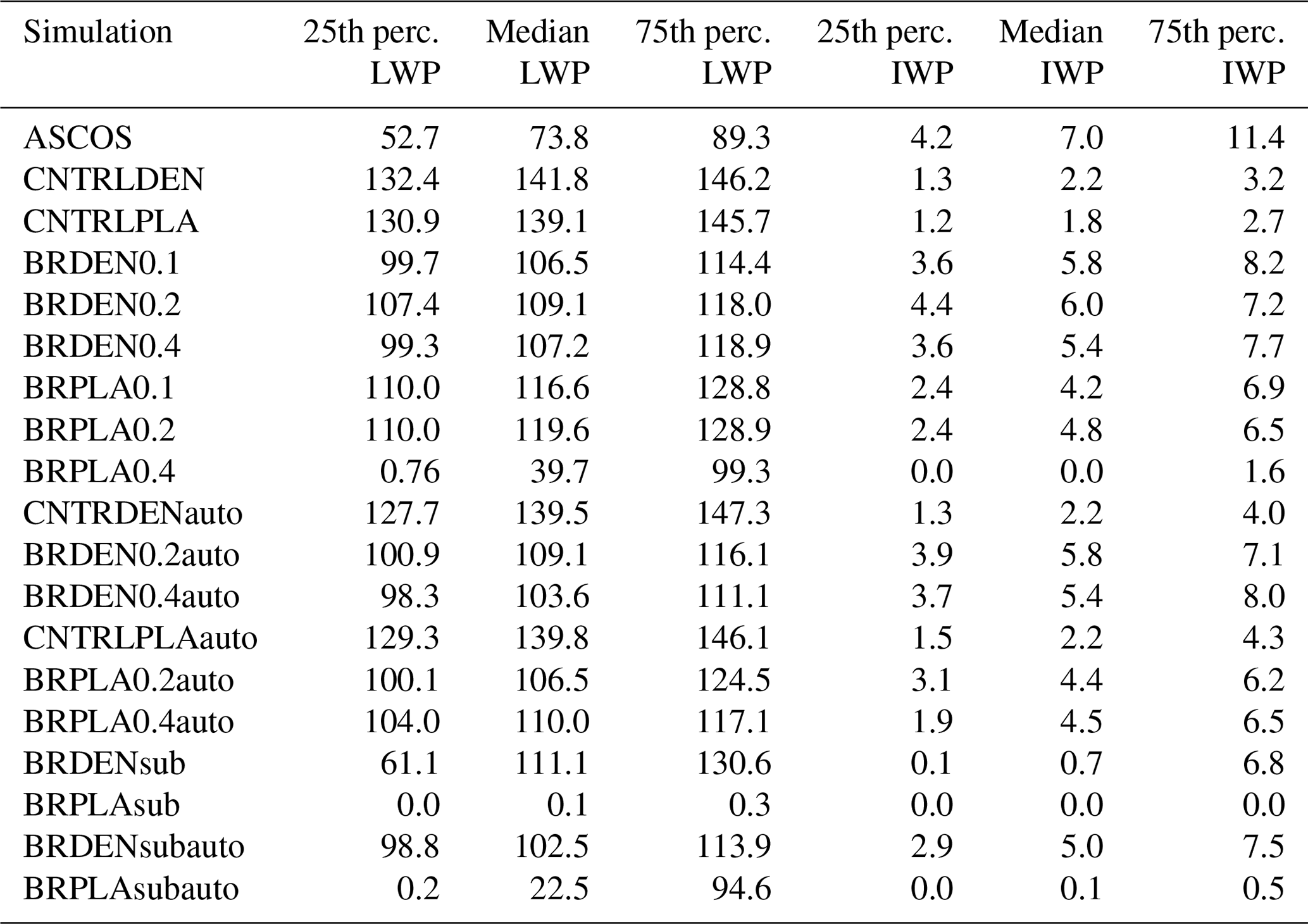
Table 3 The 25th, 50th (median) and 75th percentiles of LWP and IWP time series. All variables are in grams per square meter (g m⁻²).

3.3.3 The impact of the ice hydrometeor type

The MIMICA LES has previously been used to study ice–ice collisions in Sotiropoulou et al. (2020); however, they used a parcel-model-based parameterization of the process instead of implementing a breakup parameterization as a part of the MIMICA microphysics scheme. Sotiropoulou et al. (2020) argued that the efficiency of the process is likely underestimated in bulk microphysics schemes, in which the dynamics of the ice particle spectrum is poorly represented and fixed particle properties are assumed typically for three ice types (cloud ice, graupel, snow), which is rather unrealistic. Their argument might be particularly true for the studied case in which no snow is produced in the simulations with dendrites (Fig. S1d).

An interesting finding in Stevens et al. (2018), who compared the performance of several models that simulated the present case, was that the dominant ice particle type can be highly variable among the different models. For example, COSMO-LES and the Weather and Research Forecasting (WRF) model contain only a single ice particle category, which is cloud ice and snow, respectively. MIMICA simulates both graupel and cloud ice, with the former being substantially more abundant for the present case. COSMO-NWP (numerical weather prediction model) and UM-CASIM (the Met Office Unified Model with Cloud AeroSol Interacting Microphysics model) simulate snow and cloud ice. Cloud ice number concentrations were very limited in COSMO-NWP, while they were comparable to snow concentrations in UM-CASIM. These differences in ice particle properties result in very different ice water content (IWC) (see Fig. 11 in Stevens et al., 2018) and can likely affect the efficiency of the breakup process. Nevertheless, MIMICA is the model that predicts more realistic IWC values in the study by Stevens et al. (2018), while most models (except UM-CASIM) predict very little ice content.

The main reason why MIMICA favors graupel formation is because all cloud ice particles with sizes larger than 150 µm that collide with droplets are added to this category. This is not the same in other schemes; e.g., Morrison et al. (2005) consider that once cloud droplets are accreted on cloud ice, the rimed particle remains in the same ice category. However, adapting this approach in our model resulted in substantial enhancement of the cloud ice content and eventually to cloud glaciation (not showed). This indicates that different bulk microphysics schemes are tuned in very different ways. Another difference is that MIMICA allows for snow formation only through aggregation of cloud ice particles, while other microphysics schemes (Morrison et al., 2005; Morrison and Gettelman, 2008) also consider that cloud ice particles can grow to snowflakes through vapor deposition.

To test how differences in cloud ice content distribution among different hydrometeor types affect the multiplication efficiency of breakup, we further implemented a description for cloud-ice-to-snow autoconversion (Appendix C) assuming that ice crystals with diameters larger than 500 µm are converted to snow. These simulations are referred to as CNTRLDENauto, BRDEN0.2auto and BRDEN0.4auto for dendritic cloud ice and snow and CNTRLPLAauto, BRPLA0.2auto and BRPLA0.4auto when a non-dendritic planar ice habit is assumed. The number 0.2 or 0.4 indicates the prescribed rimed fraction. Tests with a lower separation diameter for cloud ice and snow showed little sensitivity to the choice of this parameter. In addition to the cloud-ice-to-snow autoconversion description given in Appendix C, we also tested a different parameterization following Ferrier (1994). In order to conserve the highest moments of the ice particle spectra, this parameterization assumes that the amount of cloud ice is approximately constant by converting a few large ice crystals into snow. Yet, activating this process had very little impact on the macrophysical properties in simulations with inactive and active BR. While the results of this set of simulations are not shown, the reasons for a variable sensitivity to different descriptions of the autoconversion process are discussed in the text.

3.3.4 The impact of sublimation correction factor

As already discussed in Sect. 1, the laboratory data used to develop the existing parameterization (Vardiman, 1978; Takahashi et al., 1995) for breakup do not represent realistic in-cloud conditions. Phillips et al. (2017a) have attempted to quantify the impact of the simplifications in the laboratory setups. However, there is still significant uncertainty in the developed parameterization. For example, the correction factor induced in the fragility coefficient to account for the effects of sublimation on data from Vardiman (1978) was derived by the measurements of Takahashi et al. (1995) which were performed in near-saturated conditions. This factor is thus highly uncertain and can substantially reduce the number of generated fragments (see Figs. 4–6 in Phillips et al., 2017a). To test the impact of this empirical correction, two simulations are performed in which this factor has been removed from the BR parameterization. These are referred to as BRDENsub and BRPLAsub in the text (see Table 2). Finally, this modification is tested in conditions with enhanced snow formation, which are imposed by activating the cloud-ice-to-snow autoconversion process (see Sect. 3.3.3): these additional tests are referred to as BRDENsubauto and BRPLAsubauto (Table 2). The rimed fraction in all these setups is set to 0.2.

4 Results

4.1 Sensitivity to ice habit and rimed fraction

The impact of the assumed ice habit and rimed fraction in the predicted liquid and ice water paths (LWP, IWP) is presented in Fig. 2, while the median and interquartile statistics are summarized in Table 3. To quantify breakup efficiency, fragment generation rates (P_BR) for the different collision types are shown in Fig. 3 (see Appendix B for detailed formulas). P_BR results are only presented for cloud-ice–graupel, graupel–snow and snow–snow collisions since we find negligible contributions from cloud-ice–cloud-ice, cloud-ice–snow and graupel–graupel collisions.

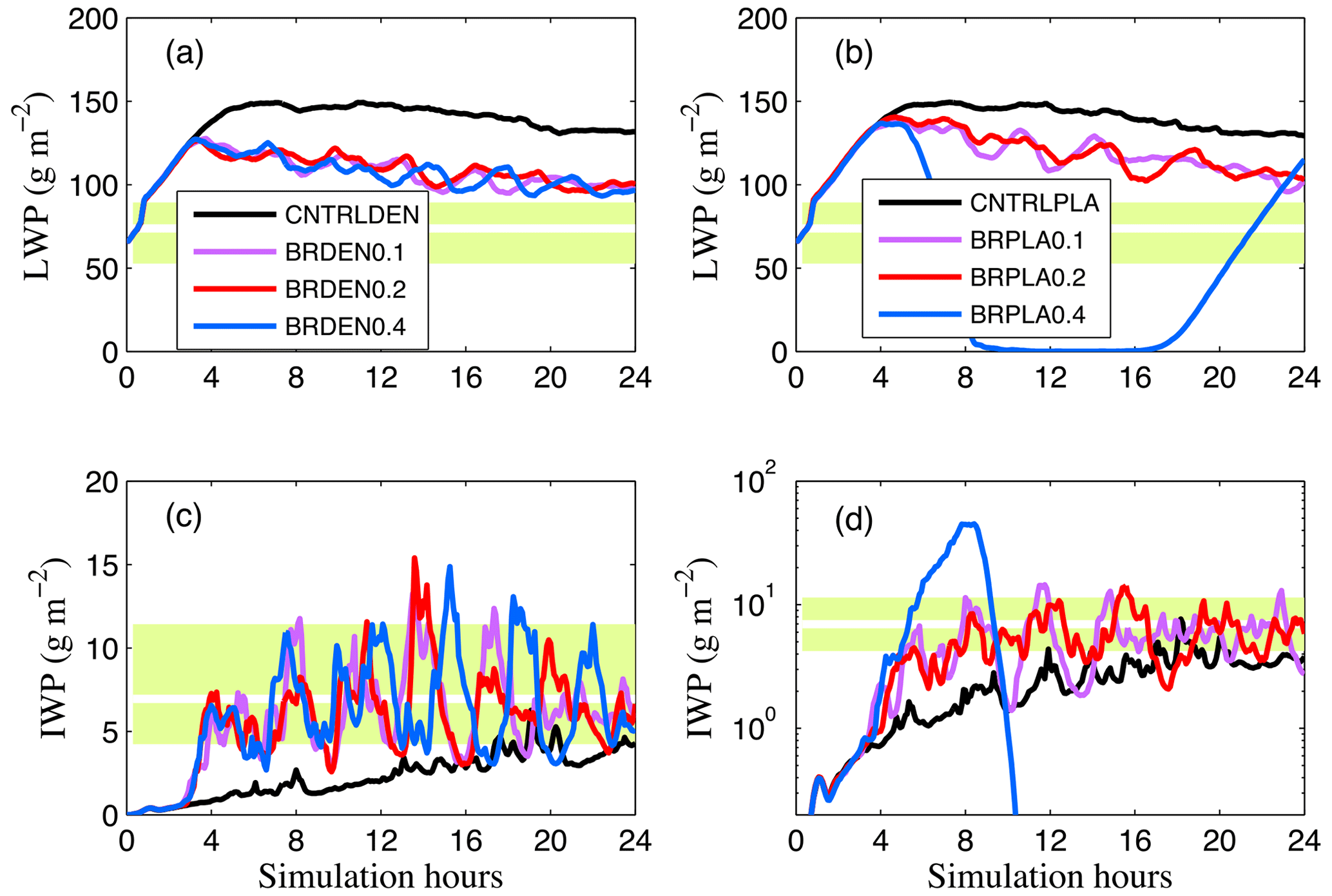
Figure 2 Time series of (a, b) LWP and (c, d) IWP for simulations with (a, c) dendrites and (b, d) plates. Light green shaded area indicates the interquartile range of observations, while the horizontal white line shows median observed values. Black lines represent simulations that account only for PIP. Purple, red and blue lines represent simulations with active breakup and a prescribed rimed fraction of 0.1, 0.2 and 0.4, respectively, for the cloud ice and snowflakes that undergo breakup. Note the logarithmic y scale in panel (d).

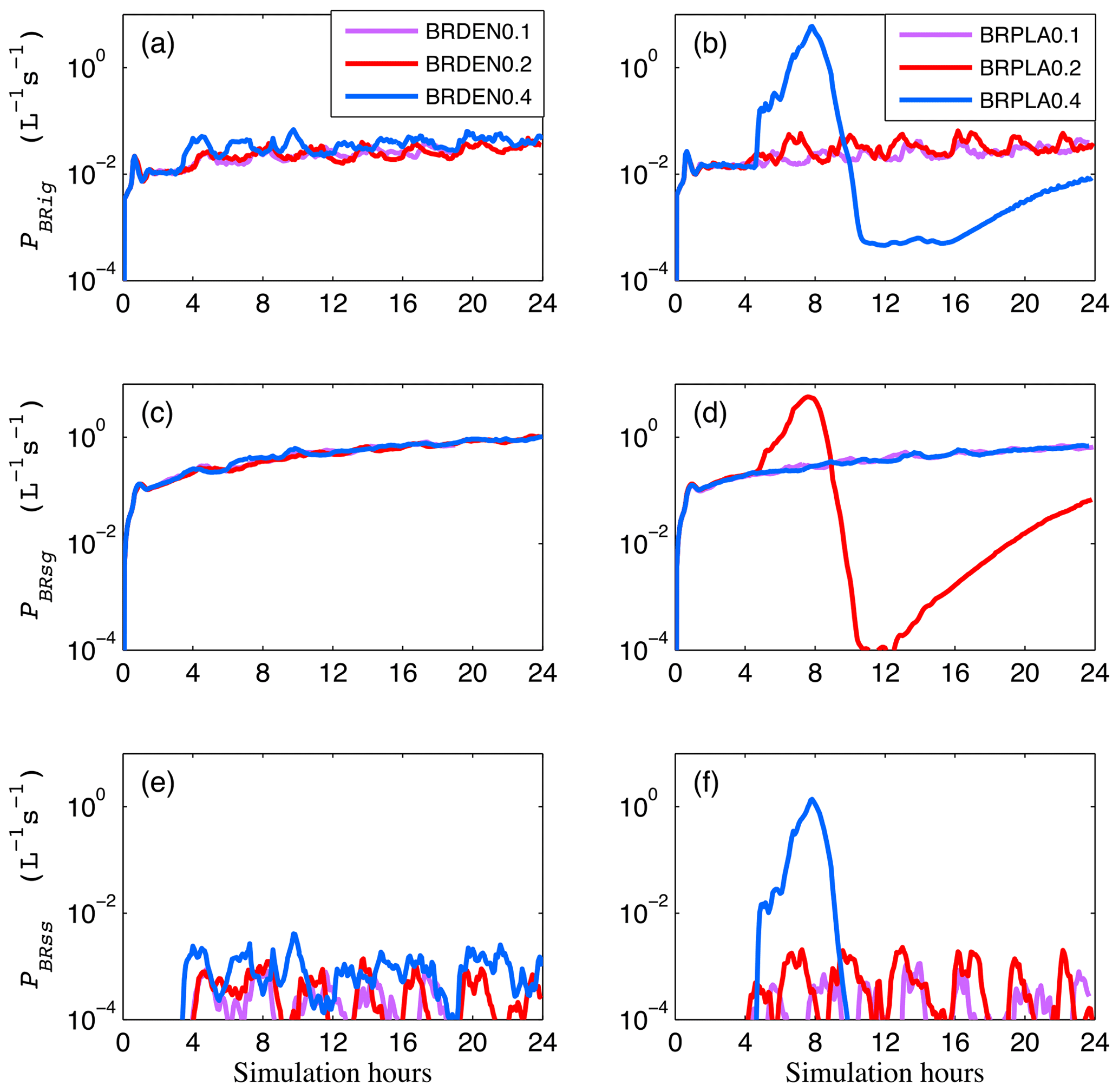
Figure 3 Time series of domain-averaged fragment generation rate (L⁻¹ s⁻¹) from (a, b) cloud-ice–graupel (P_BRig), (c, d) snow–graupel (P_BRsg) and (e, f) snow–snow (P_BRss) collisions for simulations with varying rimed fractions for cloud ice and snow: 0.1 (purple), 0.2 (magenta) and 0.4 (blue). Panels (a), (c) and (e) correspond to simulations with dendrites and (b), (d) and (f) with plates. Note the logarithmic y scale.

Small differences are observed in the integrated cloud water quantities between CNTRLDEN and CNTRLPLA as both produce median LWP values between 139–143 g m⁻² and median IWP values of 1.8–2.2 g m⁻². Hence, both simulations overestimate cloud liquid (Fig. 2a, b) and underestimate ice compared to observations (Fig. 2c, d). Specifically, the median observed LWP (73.8 g m⁻²) is overestimated by almost a factor of 2, while IWP (7 g m⁻²) is underestimated by about a factor of 3–3.5 (Table 3), which is larger than the uncertainty in the observations.

Activating breakup for dendrites results in improved simulated water properties: median LWP (IWP) decreases (increases) by 32–36 (2.2–3.8) g m⁻², with differences in the assumed rimed fraction having a weak impact on the results (Fig. 2a, c). The total fragment generation rates in Fig. 3 indicate that ice multiplication is dominated by snow–graupel collisions in these simulations. It is interesting that while snow is not formed in the CNTRLDEN simulation (Fig. S2), activation of breakup enhances cloud ice concentrations and thus the frequency of collisions between them, which promotes snow formation; breakup of snow eventually dominates the multiplication process (Fig. 3a, c, e). Generally, all total fragmentation rates in simulations with dendrites remain below 1.1 (L⁻¹ s⁻¹) with small differences for different assumptions in Ψ (Fig. 3a, c, d).

Simulations with plates and a rimed fraction ≤0.2 produce similar macrophysical properties (Fig. 2b, d); LWP (IWP) decreases (increases) by 20–25 (2.4–2.6) g m⁻², suggesting lower efficiency of breakup compared to simulations with dendrites. This is also indicated by the lower fragment generation rates, which reach a maximum value of 0.8 (L⁻¹ s⁻¹) at the end of BRPLA0.1 and BRPLA0.2 simulations (Fig. 3b, d, e). However, the cloud in BRPLA0.4 rapidly dissipates after 8 h owing to excessive multiplication, with the total P_BR reaching a maximum of 12.8 L⁻¹ s⁻¹ (Fig. 3b, d, f). Yet, a supercooled liquid cloud reforms after 15 h; LWP increases again to values larger than 100 g m⁻² by the end of the simulated period (Fig. 2b), while IWP remains close to zero (Fig. 2d). Our findings are in agreement with Loewe et al. (2018) who showed that a prescribed ICNC value of 10 L⁻¹ can lead to cloud dissipation for the specific case study.

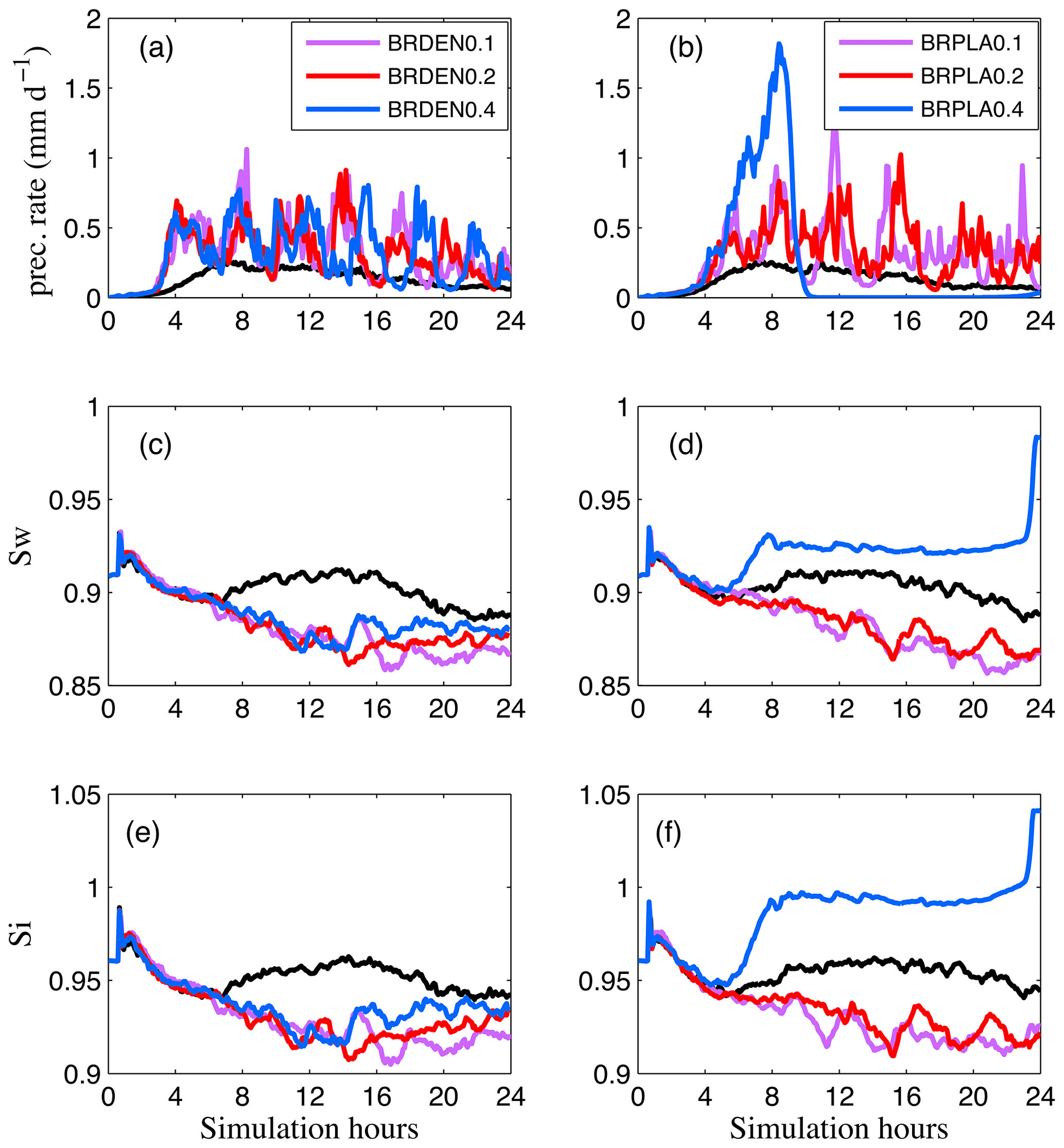
Figure 4 Time series of domain-averaged (a, b) surface precipitation rate (mm d⁻¹) and sub-cloud minimum saturation with respect to (c, d) water and (e, f) ice. The black line corresponds to the simulation without active breakup. In the rest of the simulations, rimed fraction is set to 0.1 (purple), 0.2 (magenta) and 0.4 (blue). Panels (a), (c) and (e) correspond to simulations with dendrites and (b), (d) and (f) with plates.

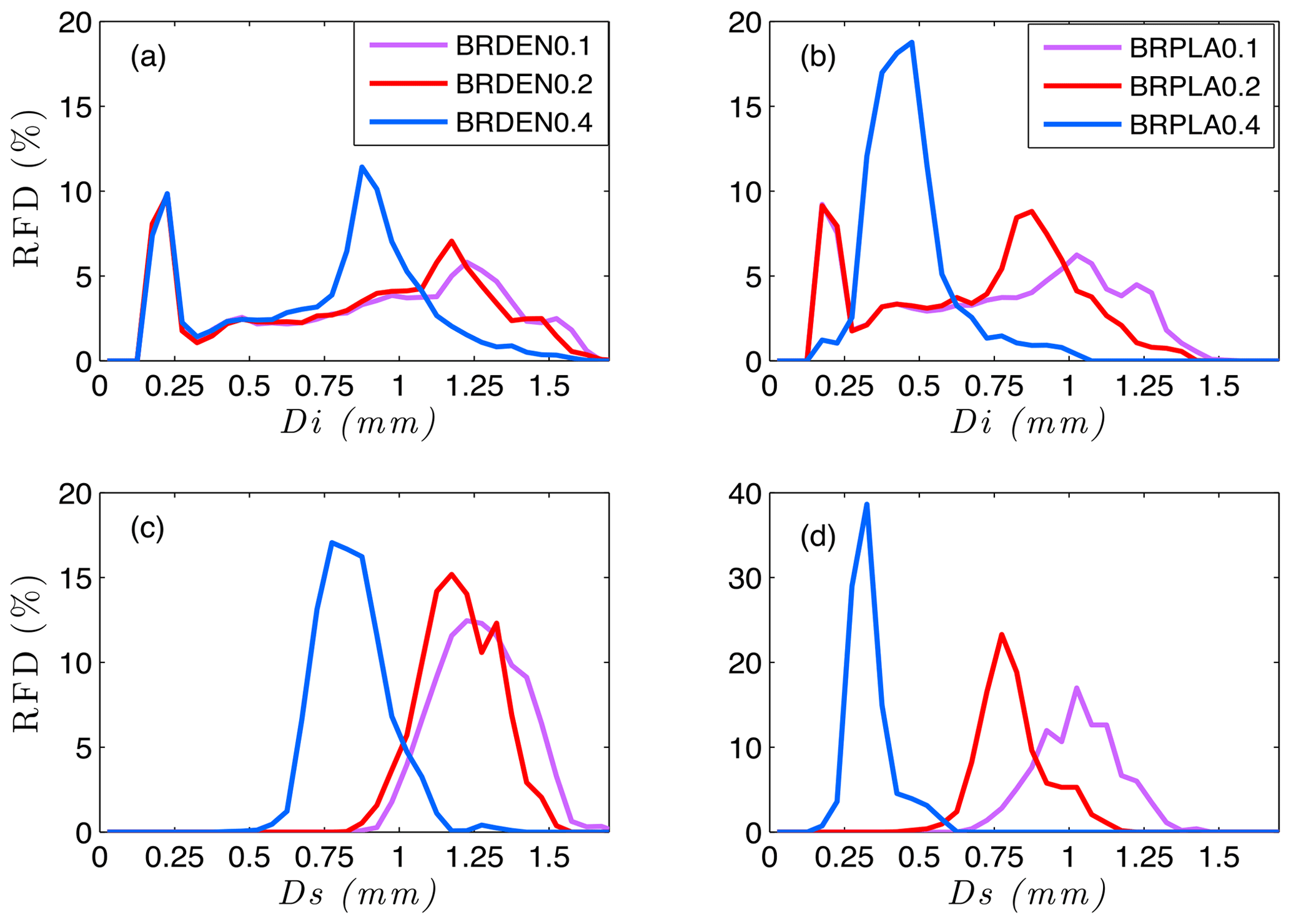
Figure 5 Relative frequency distribution (RFD) of the mean (a, b) cloud ice and (c, d) snow diameter for simulations with (a, c) dendrites and (b, d) plates. Purple, red and blue lines correspond to a prescribed rimed fraction of 0.1, 0.2 and 0.4 for the cloud ice and snow particles than undergo breakup. Calculations are performed offline based on the domain-averaged cloud ice and snow concentrations.

Analysis of the simulation results indicates strong feedbacks between fragment generation, precipitation and evaporation or sublimation within the subcloud layer. To facilitate the discussion of these feedbacks, time series of mean surface precipitation rates and minimum sub-cloud saturation values are presented in Fig. 4, while the relative frequency distributions (RFDs) of the characteristic diameters of cloud ice and snow particles are shown in Fig. 5. Precipitation rates increase when breakup is activated (Fig. 4a, b), resulting in an overall lower total condensate. Moreover, saturation with respect to both liquid (Fig. 4c, d) and ice (Fig. 4e, f) decreases in all these simulations, except in BRPLA0.4, as increasing precipitation depletes the available water vapor in the subcloud layer. This process further enhances the reduction of the total water path (LWP + IWP). An opposite behavior is only found in BRPLA0.4 (Fig. 5d, f); the continuous multiplication shifts ice particle distributions to substantially smaller sizes (Fig. 5b, d) that can sublimate more efficiently in the sub-cloud layer. The feedbacks between breakup efficiency and changes in the simulated particle size distributions are discussed in more detail below.

The RFDs of the cloud ice diameter exhibit a bimodal distribution for all simulations with dendrites (Fig. 5a). This is due to the fact that cloud-ice-to-snow autoconversion is not treated in the default MIMICA model, and ice crystals are allowed to grow to precipitation sizes without any size limits. Such precipitation-sized particles are represented by the second mode that corresponds to a size range similar to that for snow particles (Fig. 5c). The first mode of the cloud ice RFD does not play a significant role in the ice multiplication process due to the small sizes ∼ 200–250 µm; this is proven by the fact that the characteristics of this mode do not change among the different simulations. On the contrary, with increasing rime fraction and thus increasing fragment generation, the second mode (that undergoes breakup) shifts to smaller sizes. While the assumption of a constant Ψ for this rather broad RFD is unrealistic, the fact that only a certain size range of cloud ice undergoes breakup makes this simplification more reasonable. Also the comparable sizes of this cloud ice mode with snowflakes justify the adoption of the same Ψ for both ice types. Moreover, the increased fragment generation due to increasing Ψ is likely partly compensated for by the shift to smaller cloud ice and snow sizes, which are in turn expected to generate less fragments; this may explain the comparable fragmentation rates for all BRDEN setups (Fig. 3a, c, e).

The above conclusions also hold for simulations with plates and Ψ≤0.2. In BRPLA0.4 the fragment generation completely changes the RFD shape, resulting in a monomodal distribution with a substantially narrower range (Fig. 5b). Now all cloud particles can contribute to multiplication when they are not efficiently depleted by precipitation, resulting in explosive ice production. Thus for such large changes in the shape of the RFD, the assumption of a constant Ψ throughout the simulation cannot be held, and overestimations of this property can result in significant errors in cloud representation (Fig. 2b, d). While some atmospheric models explicitly predict rimed fraction (Morrison and Milbrandt, 2015), such a detailed treatment is unlikely to be adapted in coupled general circulation models (GCMs) for which minimizing computational costs is critical.

Generally, BR efficiency is found to be weak for the examined conditions as ICNC enhancement rarely exceeds a factor of 2 in most simulations (Fig. 6a, b). This is substantially lower than the 10–20 fold enhancement found in Sotiropoulou et al. (2020, 2021) for warmer mixed-phase clouds. However, note that an ICNC increase larger than a factor of 10, as in BRPLA0.4, would lead to cloud glaciation in the examined conditions (Fig. 6b). Yet this 1.5–2 fold ICNC enhancement (Fig. 6a, b) is qualitatively consistent with in situ Arctic cloud observations by Rangno and Hobbs (2001) who found that 35 % of the observed ice particles where likely produced by fragmentation upon ice particle collisions. It is interesting that a weak ICNC increase can enhance IWP by a factor of ∼5 and ∼3.3 in simulations with dendrites (Fig. 6c) and plates (Fig. 6d), respectively; this enhancement becomes gradually weaker after 12 h of simulation, stabilizing to a factor of 2. This is likely due to a feedback between BR efficiency and ICNC concentrations; as ICNCs increase with time, the size spectra is shifted to smaller sizes characterized by lower breakup efficiency. Overall, activation of breakup results in a realistic IWP, while small improvements are found in the liquid properties; LWP remains above the observed interquartile range (Fig. 2a, b). Stevens et al. (2018) showed that simulations with interactive aerosols produce less LWP for the examined case compared to simulations with a fixed background CCN concentration. Thus deviations between the simulated and observed LWPs could be attributed to the simplified aerosol treatment rather than to inadequacies in the representation of the breakup process.

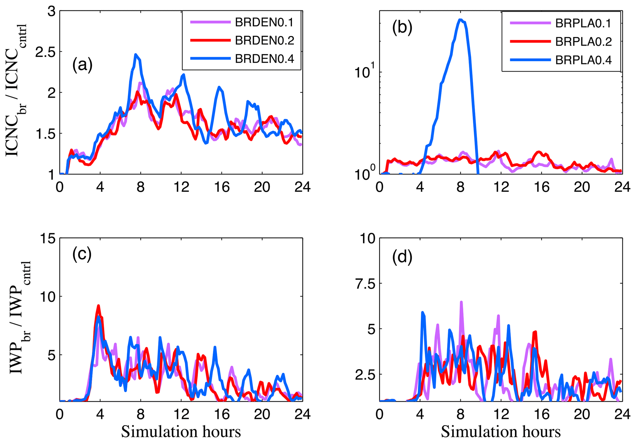
Figure 6 Time series of domain-averaged (a, b) ICNC and (c, d) IWP enhancement due to breakup. ICNC (IWP) enhancement is calculated by dividing the total ICNCs produced in each simulation with active ice multiplication with those produced by the control experiment that accounts only for PIP. The rimed fraction of cloud ice and snowflakes that undergo breakup is set to 0.1 (purple), 0.2 (magenta) and 0.4 (blue). Panels (a) and (c) correspond to simulations with dendrites and (b) and (d) with plates.

4.2 Sensitivity to snow formation

Ice multiplication generally shifts cloud ice size distributions to smaller values. In simulations with moderate fragment generation, precipitation processes can balance continuous fragment generation due to breakup (Fig. 2). However, in BRPLA0.4 the larger fragment generation cannot be counterbalanced by precipitation, resulting in continuous accumulation of cloud ice particles within the cloud layer until the cloud glaciates. This is indicated by the lack of the bimodal shape in the RFD for BRPLA0.4 presented in Fig. 5b. However, this behavior can largely be supported by the fact that cloud-ice-to-snow autoconversion is not treated in the default MIMICA version, which can enhance snow formation and thus precipitation.

Activation of autoconversion in simulation setups that do not account for breakup has hardly any impact on IWP and LWP properties (Fig. 7). LWP and IWP statistics are similar between CNTRLPLA–CNTRPLAauto and CNTRLDEN–CNTRDENauto. The same holds for simulations with dendrites and active breakup. BRPLA0.2auto produces somewhat improved LWP (reduced by ∼13 g m⁻² compared to BRPLA0.2; Table 3), while the improvements are substantially larger in BRPLA0.4auto. The hypothesis that the implementation of cloud-ice-to-snow autoconversion in the model can prevent the cloud glaciation occurring in BRPLA0.4 is confirmed in this simulation, and the LWP and IWP statistics produced are similar to BRPLA0.2auto. However, this behavior is not the same for all autoconversion schemes: application of the formulation described in Ferrier (1994) does not prevent cloud dissipation (not shown). This is because Ferrier (1994) assume that only very few large ice crystals are converted to snow and that the number concentration in the cloud ice category remains unaffected. To prevent explosive multiplication in this setup, a reduction in cloud ice number concentration is essential.

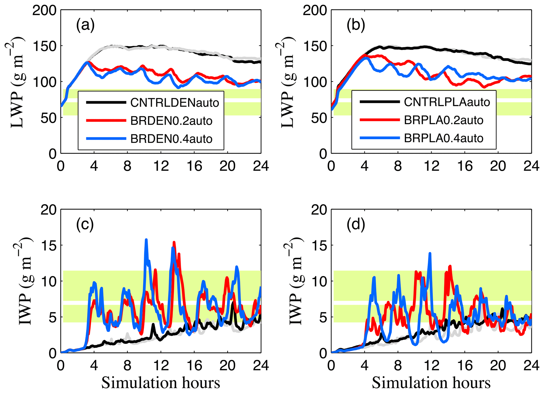
Figure 7 Same as Fig. 2 but for simulations with active cloud-ice-to-snow autoconversion. The cloud ice habit is set to (a, c) dendrites and (b, d) plates. Black lines represent simulations that account only for PIP. Red lines include the breakup process with a prescribed rimed fraction for cloud ice and snow set to 0.2. Blue lines are similar to red but with the prescribed fraction set to 0.4. Light grey lines represent baseline simulations that do not account for autoconversion: (a, c) CNTRLDEN and (b, d) CNTRLPLA (see Table 2).

Note that while with active breakup the model still does not reproduce liquid and ice partitioning correctly, there are significant improvements compared to the standard code. While CNTRLDENauto fails completely to reproduce the relationship between LWP and IWP (Fig. 8a, b), activation of breakup results in a partial agreement between modeled and observed LWP-IWP fields (Fig. 8a, c, d). Improvements of liquid–ice partitioning are also evident in BRPLA0.2auto and BRPLA0.4auto compared to CNTRLPLAauto (Fig. 9), with BRPLA0.2auto being in better agreement with ASCOS observations. However, there are still significant deviations particularly in the representation of the liquid condensate which can be linked either to an underestimate in the ice production or to the simplified treatment of aerosols that act as CCN (Stevens et al., 2018).

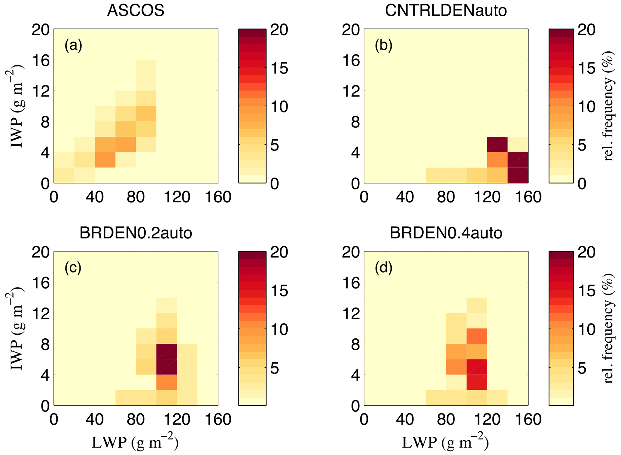
Figure 8 Relative frequency distribution of IWP (g m⁻²) as a function of LWP (g m⁻²) for (a) ASCOS, (b) CNTRLDENauto, (c) BRDEN0.2auto and (d) BRDEN0.4auto (see Table 2). Cloud-ice-to-snow autoconversion is active in all model simulations. Collisional breakup is included only in panels (c) and (d) with the cloud ice and snow rimed fraction set to (c) 0.2 and (d) 0.4. In all simulations a dendritic cloud ice habit is assumed.

4.3 Sensitivity to the sublimation correction factor

In Sect. 4.1, simulations with plates were found to be more sensitive to increases in fragment generation induced by changes in the prescribed Ψ. In particular, ICNC enhancements of a factor of 10 resulted in cloud glaciation (Fig. 6b). Here we further examine the sensitivity of the results to increased ice multiplication by removing the correction factor for sublimation effects adapted in the Phillips et al. (2017a) parameterization. For lightly rimed particles (Ψ=0.2), the reduction in fragment generation induced by this factor is largely variable depending on the collision type (see Figs. 4b and 5a in Phillips et al., 2017b).

Both BRDENsub and BRPLAsub simulations result in explosive ice multiplication and cloud dissipation (Fig. 10). In BRDENsub the cloud almost disappears after 6.5 h and reforms after 8.5 h (Fig. 10a). In BRPLAsub the cloud glaciates within 4 h, and cloud-free conditions prevail for the rest of the simulation time (Fig. 10b). Activation of cloud-ice-to-snow autoconversion for this setup prevents ice explosion and cloud dissipation in the simulation with dendrites but not with plates. In BRPLAsubauto, the autoconversion process only delays cloud glaciation by 3 h. Overall, the removal of the correction factor results in poorer agreement with observations (Table 3). This indicates that while the determination of the correction factor is highly uncertain, its inclusion in the breakup parameterization is essential when applied to polar stratocumulus clouds, particularly in the case of non-dendritic planar ice. The high sensitivity that simulations exhibit to this parameter suggests that possible errors in the estimation of the correction factor can have a large impact on the multiplication effect predicted by the parameterization of Phillips et al. (2017a), particularly in conditions that favor the formation of non-dendritic planar ice.

Figure 9 Relative frequency distribution of IWP (g m⁻²) as a function of LWP (g m⁻²) for (a) ASCOS, (b) CNTRLPLA, (c) BRPLA0.2auto and (d) BRPLA0.4auto (see Table 2). The setup in each panel is similar to Fig. 8 except that in all simulations a planar cloud ice habit is assumed.

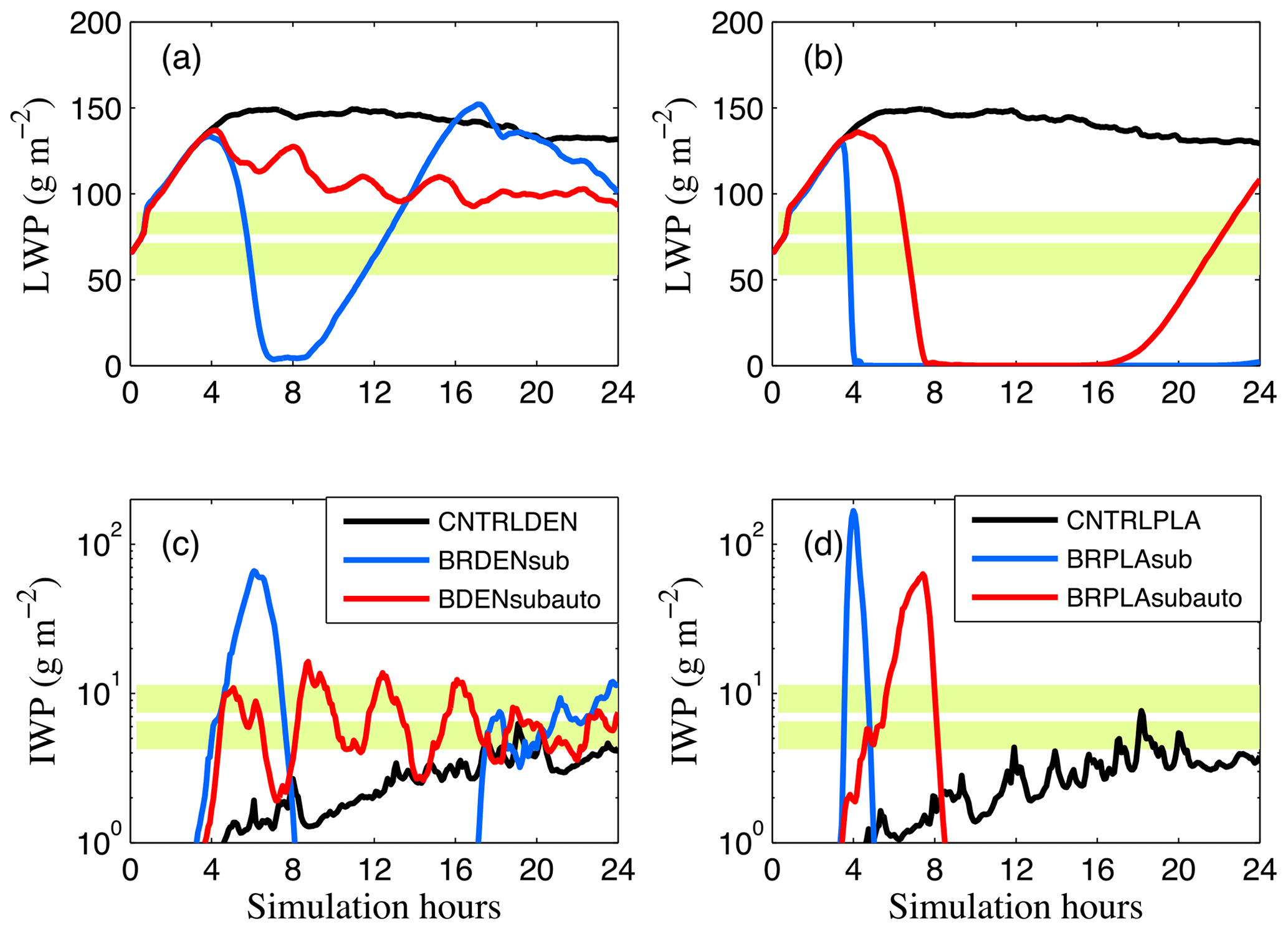
Figure 10 Similar to Fig. 2 but for simulations that do not include the sublimation correction factor in the breakup parameterization. Cloud-ice-to-snow autoconversion is active in BRDENsubauto and BRPLAsubauto simulations. Rimed fraction is set to 0.2.

5 Discussion

Ice formation processes in Arctic clouds are sources of great uncertainty in atmospheric models, often resulting in underestimation of the cloud ice content compared to observations. The poor representation of SIPs has been suggested as the main cause behind this underestimation (Fridlind and Ackerman, 2019) as rime splintering is usually the only multiplication mechanism described in models. In situ observations (Rangno and Hobbs, 1991; Schwarzenboeck et al., 2009) and recent modeling studies (Sotiropoulou et al., 2020, 2021) suggest that collisional breakup is likely critical in polar mixed-phase clouds. However, due to the limited availability of laboratory studies and the unrealistic setups utilized in them (Vardiman, 1978; Takahashi et al., 1995), the parameterization of this process is particularly challenging. Phillips et al. (2017a, b) have recently developed a physically based numerical description for collisional breakup, constrained with existing laboratory data. This scheme estimates the number of fragments as a function of collisional kinetic energy, environmental temperature, size and rimed fraction of the particle that undergoes breakup, while the influence of the different ice types and ice habits are also accounted for.

While being more advanced than any other description for collisional breakup (e.g., Sullivan et al., 2018), the details of this parameterization cannot be addressed in most bulk microphysics schemes. While microphysics schemes with explicit prediction of the ice habit (e.g., Jensen et al., 2017) or rimed fraction (e.g., Morrison and Milbradt, 2015) have been developed, such detailed treatments are not utilized in coupled climate models as computational cost must be minimized. Thus the representation of the breakup process in these models requires some simplifications. In this study we attempt to quantify the impact of ice multiplication through collisional breakup in summertime high-Arctic conditions and examine the sensitivity of the efficiency of this process to assumptions in the ice habit and rimed fraction of the colliding particles. We also examine how changes in ice type affect the multiplication process through the activation of cloud-ice-to-snow autoconversion, a process not represented in the default model.

Simulations with a dendritic ice habit produce a realistic IWP when breakup is activated. The results show little sensitivity to assumptions in rimed fraction, suggesting that the lack of a prognostic treatment of this parameter in most bulk microphysics schemes is not detrimental for the description of the breakup process. Note that increases in Ψ result in increased ice multiplication that shifts the ice particle size distribution towards smaller values. These smaller particles can generate fewer fragments, which compensate for the enhancing effects of the larger Ψ. LWP is also somewhat improved compared to the simulation that does not account for SIPs; however, it still remains higher than the observed interquartile range.

Ice multiplication also improves the macrophysical state of the cloud in simulations with plates as long as the cloud ice and snow particles that undergo breakup are assumed to be lightly rimed. These improvements are slightly smaller compared to the simulations with dendrites. However, prescribing a high rimed fraction for plates results in explosive multiplication if cloud-ice-to-snow autoconversion is not accounted for in the model. This is because the larger fragment generation rates are not balanced by precipitation processes and the freshly formed small fragments accumulate in the cloud ice category, continuously feeding the multiplication process until the cloud glaciates.

Since fragment generation in the parameterization by Phillips et al. (2017a, b) is constrained based on unrealistic laboratory setups, there is considerable uncertainty in the estimated number of fragments. The impact of the correction for sublimation effects in the data of Vardiman (1978) is examined by removing the relevant correction factor. This, however, resulted in cloud glaciation in both simulations with dendrites and plates, confirming that this correction is essential to avoid an unrealistic explosive multiplication. Enhanced precipitation through the activation of cloud-ice-to-snow autoconversion can prevent cloud dissipation in all sensitivity tests that result in explosive multiplication, except for the setup with non-dendritic planar ice that does not include the sublimation correction factor.

ICNC enhancement in the most realistic simulations rarely exceeds a factor of 2. Yano and Phillips (2011) developed a metric for multiplication efficiency, Ĉ =4c₀a t_ft_g, where c₀ is the primary ice generation rate, a is the breakup rate (which is the product of the sweep-out rate and the number of fragments generated per collision), and t_f and t_g are the timescale for fallout of large ice precipitation and timescale for conversion of small to large ice precipitation, respectively. Graupel formation occurs relatively fast in our model; thus our t_g is smaller compared to the numbers adapted in previous studies (Yano and Phillips, 2011; Phillips et al., 2017b; Sotiropoulou et al., 2020): 6.6 and 7.5 min for BRPLA0.2 and BRDEN0.2 simulations, respectively. Also the number of fragments generated per snow collision is found to be larger compared to warmer Arctic conditions: Sotiropoulou et al. (2020) found that a maximum of five fragments are generated per snow–graupel collision, while up to 13.7 (8.5) fragments are produced in the BRPLA0.2 (BRDEN0.2) simulations. While observations of Arctic clouds (Schwarzenboeck et al., 2009) also indicate that breakup of an ice particle usually produces less than five fragments, these estimates are only based on the examination of particles around 300 µm or roughly larger. In our simulations, millimeter particles mainly contribute to ice multiplication (Fig. 5), suggesting that the estimated fragmentation number is not unreasonable. Nevertheless, substituting these parameters in the above formula yields Ĉ =1.6 and Ĉ =2.2 for BRDEN0.2 and BRPLA0.2 simulations, which is 4.5–5.5 times lower than the estimated efficiency found in previous studies of mesoscale convective systems (Phillips et al., 2017b) and Arctic stratocumulus clouds (Sotiropoulou et al., 2020). While Ĉ >1 implies that explosive multiplication is possible (Yano and Phillips, 2011), the required time for this to happen is much longer than the time mixing scale of the studied cloud. For this reason, such low Ĉ are associated with generally weak ICNC enhancement.

Sotiropoulou et al. (2020) found a 10–20 fold enhancement in ICNCs due to breakup compared to the available INPs and estimated Ĉ =10 for Arctic clouds within the Hallet–Mossop temperature range. However, their case is characterized by lower INP concentrations that do not exceed 0.1 L⁻¹, while in sensitivity tests of primary ice nucleation they showed that increasing INPs result in decreasing secondary ice production. In the present study, relatively high INP conditions are adapted. Primary ICNCs increase with time as the cloud cools through radiative cooling, reaching a maximum of 1 L⁻¹ towards the end of the simulation. While primary ice formation in our setup is likely overestimated (Fridlind et al., 2007; Wex et al., 2019), our results support the conclusions of Sotiropoulou et al. (2020) and further suggest that as primary ice nucleation becomes more and more enhanced at colder temperatures, ice multiplication from ice–ice collisions will likely become less significant. It is interesting that while laboratory experiments from Takahashi et al. (1995), based on collisions of two hailstones, suggest increasing ice multiplication with decreasing temperature from −3 to −15 ^∘C, our findings indicate that this might not happen in the real atmosphere due to the increasing availability of INPs.

Finally, the possibility that ice multiplication is still underestimated in our simulations cannot be excluded since MIMICA predicts that only 10 %–12 % of the simulated ice particles in BRDEN0.2 and BRPLA0.2 simulations contribute to ice multiplication through breakup. Schwarzenboeck et al. (2009) found indications of fragmentation in 55 % of the examined ice particles, although natural fragmentation could only be confirmed for 18 %, while their sample was characterized by relatively small sizes. Moreover, while processes like rime splintering and drop shattering are clearly ineffective in the examined conditions, the contribution from other SIP mechanisms has not been investigated, e.g., blowing snow and fragmentation of sublimating particles (Field et al., 2017). Sublimation of cloud ice particles can occur if cloud conditions become subsaturated with respect to ice; however, a preliminary inspection of the domain-averaged supersaturation profiles did not reveal any such evidence. Furthermore, blowing snow is associated with relatively high wind speeds (Gossart et al., 2017), while during the examined ASCOS case the maximum wind speed never exceeded 5.2 m s⁻² in the boundary layer.

6 Conclusions

In this study, ice multiplication from ice–ice collisions is implemented in the MIMICA LES, following Phillips et al. (2017a, b), to investigate the role of this process for ice–liquid partitioning in a summertime Arctic low-level cloud deck observed during ASCOS. The sensitivity of the simulated results to the prescribed ice habit and rimed fraction is examined. The impact of changes in ice content distribution among the three ice categories is also investigated by accounting for cloud-ice-to-snow autoconversion and thus enhancing snow. The last set of sensitivity tests concerns the sublimation correction factor adapted in the parameterization, which is a highly uncertain parameter. Our findings can be summarized as follows:

• For the simulated temperature range (−12.5 to −7 ^∘C), ice multiplication from collisional breakup is generally weak, enhancing ICNCs by on average no more than a factor of 1.5–2 in the simulations that are most consistent with observations. Increases in ICNCs due to breakup are compensated for by increased precipitation and sublimation in the sub-cloud layer. Simulation setups that produce a 10-fold ICNC enhancement result in cloud dissipation.

• While activation of breakup can substantially improve the agreement between modeled and observed cloud ice content, the impact on cloud liquid is weaker. Ice multiplication can decrease the median LWP by 25–35 g m⁻², resulting in better agreement with observations. Yet cloud liquid content remains overestimated in the model.

• Ice multiplication from the breakup of dendrites is not very sensitive to assumptions regarding the rimed fraction. The breakup of lightly rimed non-dendritic planar ice also produces similar cloud water properties as in the simulations with dendrites. In contrast, the breakup of highly rimed plates can lead to cloud dissipation if cloud-ice-to-snow autoconversion is not accounted for in the microphysics scheme. Activating cloud-ice-to-snow autoconversion enhances the precipitation sink, which prevents accumulation of cloud ice particles, excessive multiplication and cloud dissipation.

• Removing the correction factor for sublimation effects from the Phillips et al. (2017a, b) parameterization results in cloud glaciation independent of the assumed ice habit. Activation of cloud-ice-to-snow autoconversion can prevent explosive multiplication in this setup only for simulations with dendrites. The large sensitivity of the results suggest that this factor is likely the most important source of uncertainty in the representation of breakup, especially for non-dendritic planar ice particles.

The generally low sensitivity of our results to assumptions regarding ice habit and rimed fraction indicate that the lack of an explicit prediction of these properties in climate models is not detrimental for the representation of ice multiplication effects due to breakup in Arctic clouds. The sensitivity, however, is in some setups influenced by the way snow formation is treated since snow precipitation can prevent continuous accumulation of ice particles within the cloud layer. Cloud-ice-to-snow autoconversion appears to be a key process to sustain the balance between ice sources and sinks, and this process is usually considered in most climate model bulk microphysics schemes (e.g., Murakami, 1990; Morrison and Gettelman, 2008). Finally, we acknowledge that the weak influence of the rimed fraction is likely limited for conditions characterized by weak multiplication efficiency (Ĉ ≈2) and thus weak ICNC enhancement, as those examined here. Future model development plans include the treatment of rimed fraction as a prognostic variable; this is likely important for the study of collisional breakup effects in more convective clouds.

Appendix A: Primary ice production

The immersion freezing parameterization is based on the concept of ice nucleation active site density. The formulation of Niemand et al. (2012) is used, adapted for microline dust particles (Ickes et al., 2017). It is utilized here as the only primary ice production mechanism. In this scheme, the number of nucleated ice particles (N_INP, m⁻³) is given as a function of N_CCN and temperature T (^∘C):

$$N_{\mathrm{INP}}=X{N}_{\mathrm{CCN}}\left(\mathrm{1}-e^{-\mathrm{4}\mathit{\pi }{r}^{\mathrm{2}}{n}_{\mathrm{s}}}\right),$$

where $n_{\mathrm{s}}=e^{-aT+b}$. X is the percentage of N_CCN (m⁻³) that acts as efficient INP, e.g., 50 %, 10 % and 5 % (see Sect. S1 in the Supplement), n_s (m⁻²) is the ice nucleation active site density of the INP species assumed (here microcline), and $r=\mathrm{46.5}\times {\mathrm{10}}^{-\mathrm{9}}$ m is the mean radius of the accumulation aerosol mode measured during the examined ASCOS case (Ickes et al., 2021). The temperature dependency is determined by the coefficients α=0.73 ^∘C⁻¹ and b=9.63.

Appendix B: Ice multiplication from ice–ice collisions

A bulk description of the collisional breakup process is applied, which is based on existing descriptions of the interactions between the three ice particle types (cloud ice, snow and graupel) and within the same category (Wang and Chang, 1993). Ice multiplication is allowed after cloud-ice–cloud-ice, cloud-ice–snow, cloud-ice–graupel, graupel–snow, snow–snow and graupel–graupel collisions. For collisions between different ice types, the rate of number ($P_{{\mathrm{n}}_{\mathrm{12}}}$) and mass ($P_{{\mathrm{q}}_{\mathrm{12}}}$) concentration of particle 1 that is collected by particle 2 is given as

$$\begin{array}{}\text{(B1)}& {\displaystyle }{P}_{{\mathrm{n}}_{\mathrm{12}}}={\displaystyle \frac{\mathit{\pi }}{\mathrm{4}}}\mathit{\rho }{E}_{\mathrm{col}}{N}_{\mathrm{1}}{N}_{\mathrm{2}},\text{(B2)}& {\displaystyle }{P}_{q_{\mathrm{12}}}={\displaystyle \frac{\mathit{\pi }}{\mathrm{4}}}\mathit{\rho }{E}_{\mathrm{12}}{Q}_{\mathrm{1}}{N}_{\mathrm{2}},\end{array}$$

where subscript “n” and “m” denote number- and mass- weighted parameters, respectively. N and Q refer to number and mass concentration of the particle. E_col is the collection efficiency, given as a function of temperature (K): $E_{\mathrm{col}=}\exp \left[\mathrm{0.09}\right(T-\mathrm{273.15}\left)\right]$. For self-collection, thus collisions between the same ice types, the above equations take the form

$$\begin{array}{}\text{(B3)}& {\displaystyle }{P}_{{\mathrm{n}}_{\mathrm{11}}}={\displaystyle \frac{\mathit{\pi }}{\mathrm{2}}}\mathit{\rho }{E}_{\mathrm{col}}{N}_{\mathrm{1}}{N}_{\mathrm{1}},\text{(B4)}& {\displaystyle }{P}_{q_{\mathrm{11}}}={\displaystyle \frac{\mathit{\pi }}{\mathrm{2}}}\mathit{\rho }{E}_{\mathrm{col}}{N}_{\mathrm{1}}{Q}_{\mathrm{1}}.\end{array}$$

The above equations are further used to determine collisions that result in ice multiplication by replacing the collection efficiency with the term $E^{*}=\mathrm{1}-E_{\mathrm{col}}$. This means that the collisions that do not result in aggregation are those that contribute to the SIP. Since aggregation after cloud-ice–graupel and graupel–graupel collisions does not occur, we assume that 100 % of these collisions result in multiplication: $E^{*}=\mathrm{1}$.

The Phillips et al. (2017a) parameterization allows for varying treatments of F_BR depending on the ice crystal type and habit:

$$\begin{array}{}\text{(B5)}& F_{\mathrm{BR}}=\mathit{\alpha }A\left(\mathrm{1}-\exp \left\{-{\left[{\displaystyle \frac{C{K}_o}{\mathit{\alpha }A}}\right]}^{\mathit{\gamma }}\right\}\right).\end{array}$$

$K_o=\frac{m_{\mathrm{1}}{m}_{\mathrm{2}}}{m_{\mathrm{1}}+m_{\mathrm{2}}}{\left(\mathrm{\Delta }{u}_{{\mathrm{n}}_{\mathrm{12}}}\right)}^{\mathrm{2}}$ represents collisional kinetic energy and a=πD², where D (in meters) is the size of the smaller ice particle which undergoes fracturing and α is its surface area. Both m₁ and m₂ are the masses of the colliding particles, and $\mathrm{\Delta }{u}_{{\mathrm{n}}_{\mathrm{12}}}$ is the difference in their terminal velocities. A correction is further applied in $\mathrm{\Delta }{u}_{{\mathrm{n}}_{\mathrm{12}}}$ to account for underestimates when $u_{{\mathrm{n}}_{\mathrm{1}}}\approx u_{{\mathrm{n}}_{\mathrm{2}}}$, following Mizuno et al. (1990) and Reisner et al. (1998):

$$\left|\mathrm{\Delta }{u}_{{\mathrm{n}}_{\mathrm{12}}}\right|={\left({\left(\mathrm{1.7}{u}_{{\mathrm{n}}_{\mathrm{1}}}-u_{{\mathrm{n}}_{\mathrm{2}}}\right)}^{\mathrm{2}}+\mathrm{0.3}{u}_{{\mathrm{n}}_{\mathrm{1}}}{u}_{{\mathrm{n}}_{\mathrm{2}}}\right)}^{\mathrm{1}/\mathrm{2}}.$$

A represents the number density of the breakable asperities in the region of contact. C is the asperity-fragility coefficient, which is a function of a correction term (ψ) for the effects of sublimation based on the field observations by Vardiman (1978). Exponent γ is a function of rimed fraction for collisions that include cloud ice and snow. Particularly, for non-dendritic planar ice or snow with rimed fraction Ψ<0.5 that undergoes fracturing after collisions with other ice particles,

$$\begin{array}{ll}\text{(B6)}& {\displaystyle }& {\displaystyle }A=\mathrm{1.58}\times {\mathrm{10}}^{\mathrm{7}}\left(\mathrm{1}+\mathrm{100}{\mathrm{\Psi }}^{\mathrm{2}}\right)\left(\mathrm{1}+{\displaystyle \frac{\mathrm{1.33}\times {\mathrm{10}}^{-\mathrm{4}}}{D^{\mathrm{1.5}}}}\right),{\displaystyle }& {\displaystyle }C=\mathrm{7.08}\times {\mathrm{10}}^{\mathrm{6}}\mathit{\psi },\\ {\displaystyle }& {\displaystyle }\mathit{\psi }=\mathrm{3.5}\times {\mathrm{10}}^{-\mathrm{3}},\\ {\displaystyle }& {\displaystyle }\mathit{\gamma }=\mathrm{0.5}-\mathrm{0.25}\mathrm{\Psi }.\end{array}$$

For fragmentation of dendrites, A and C are somewhat different:

$$\begin{array}{ll}\text{(B7)}& {\displaystyle }& {\displaystyle }A=\mathrm{1.41}\times {\mathrm{10}}^{\mathrm{6}}\left(\mathrm{1}+\mathrm{100}{\mathrm{\Psi }}^{\mathrm{2}}\right)\left(\mathrm{1}+{\displaystyle \frac{\mathrm{3.98}\times {\mathrm{10}}^{-\mathrm{5}}}{D^{\mathrm{1.5}}}}\right),{\displaystyle }& {\displaystyle }C=\mathrm{3.09}\times {\mathrm{10}}^{\mathrm{6}}\mathit{\psi },\\ {\displaystyle }& {\displaystyle }\mathit{\psi }=\mathrm{3.5}\times {\mathrm{10}}^{-\mathrm{3}},\\ {\displaystyle }& {\displaystyle }\mathit{\gamma }=\mathrm{0.5}-\mathrm{0.25}\mathrm{\Psi }.\end{array}$$

For graupel–graupel collisions, an explicit temperature dependency is included in the equation, while γ is constant:

$$\begin{array}{ll}\text{(B8)}& {\displaystyle }& {\displaystyle }A={\displaystyle \frac{a_o}{\mathrm{3}}}+\max \left({\displaystyle \frac{\mathrm{2}{a}_o}{\mathrm{3}}}-{\displaystyle \frac{a_o}{\mathrm{9}}}\left|T-\mathrm{258}\right|,\mathrm{0}\right),{\displaystyle }& {\displaystyle }{a}_o=\mathrm{3.78}\times {\mathrm{10}}^{\mathrm{4}}\times \left(\mathrm{1}+{\displaystyle \frac{\mathrm{0.0079}}{D^{\mathrm{1.5}}}}\right),\\ {\displaystyle }& {\displaystyle }C=\mathrm{6.3}\times {\mathrm{10}}^{\mathrm{6}},\\ {\displaystyle }& {\displaystyle }\mathit{\psi }=\mathrm{3.5}\times {\mathrm{10}}^{-\mathrm{3}},\\ {\displaystyle }& {\displaystyle }\mathit{\gamma }=\mathrm{0.3}.\end{array}$$

The parameterization was developed based on particles with diameters 500 µm <D<5 mm; however, Phillips et al. (2017a) suggest that it can be used for particle sizes outside the recommended range as long as the input variables to the scheme are set to the nearest limit of the range. Moreover, an upper limit for the number of fragments produced per collision is imposed, set to $F_{{\mathrm{BR}}_{\max }}=\mathrm{100}$ (Phillips et al., 2017a), for all collision types. The production rate of fragments is estimated using Eq. (B1) or Eq. (B3) and one of the proposed formulations for F_BR above, e.g., $P_{{\mathrm{n}}_{\mathrm{12}}}{F}_{\mathrm{BR}}$. Whenever mass transfer also occurs, for example, if we assume that fragments ejected from snow–graupel collisions are added to the cloud ice category, we assume that this is only 0.1 % of colliding mass (Eq. B2 or Eq. B4) that undergoes breakup (Phillips et al., 2017a).

Appendix C: Cloud-ice-to-snow autoconversion

For cloud-ice-to-snow autoconversion, we use the formula adapted in Wang and Chang (1993) for cloud-ice-to-graupel and graupel-to-hail autoconversions:

$$\begin{array}{c}{\displaystyle }{P}_{q_{\mathrm{auto}}}=Q_{\mathrm{i}}{e}^{D_{\mathrm{c}}\mathit{\lambda }}\left\{\mathrm{1}+D_{\mathrm{c}}\mathit{\lambda }\left[\mathrm{1}+D_{\mathrm{c}}\mathit{\lambda }\left(\mathrm{0.5}+{\displaystyle \frac{D_{\mathrm{c}}\mathit{\lambda }}{\mathrm{6}}}\right)\right]\right\},\\ {\displaystyle }{P}_{{\mathrm{n}}_{\mathrm{auto}}}=N_{\mathrm{i}}{e}^{D_{\mathrm{c}}\mathit{\lambda }}\left(\mathrm{1}+D_{\mathrm{c}}\mathit{\lambda }\right),\end{array}$$

where $\mathit{\lambda }={\left[\frac{A_{\mathrm{m}}\mathrm{\Gamma }\left(\mathit{\alpha }+b_{\mathrm{m}}+\mathrm{1}\right)N_{\mathrm{i}}}{\mathrm{\Gamma }\left(\mathit{\alpha }+\mathrm{1}\right)Q_{\mathrm{i}}}\right]}^{\mathrm{1}/b_{\mathrm{m}}}$ and D_c is the critical diameter that separates the two ice categories. N_i and Q_i are the number and mass cloud ice concentrations, respectively.