Investigations on the anthropogenic reversal of the natural ozone gradient between northern and southern midlatitudes

Our quantitative understanding of natural tropospheric ozone concentrations is limited by the paucity of reliable measurements before the 1980s. We utilize the existing measurements to compare the long-term ozone changes that occurred within the marine boundary layer at northern and southern midlatitudes. Since 1950 ozone concentrations have increased by a factor of 2.1 ± 0.2 in the Northern Hemisphere (NH) and are presently larger than in the Southern Hemisphere (SH), where only a much smaller increase has occurred. These changes are attributed to increased ozone production driven by anthropogenic emissions of photochemical ozone precursors that increased with industrial development. The greater ozone concentrations and increases in the NH are consistent with the predominant location of anthropogenic emission sources in that hemisphere. The available measurements indicate that this interhemispheric gradient was much smaller and was likely reversed in the pre-industrial troposphere with higher concentrations in the SH. Six Earth system model (ESM) simulations indicate similar total NH increases (1.9 with a standard deviation of 0.3), but they occurred more slowly over a longer time period, and the ESMs do not find higher pre-industrial ozone in the SH. Several uncertainties in the ESMs may cause these model–measurement disagreements: the assumed natural nitrogen oxide emissions may be too large, the relatively greater fraction of ozone injected by stratosphere–troposphere exchange to the NH may be overestimated, ozone surface deposition to ocean and land surfaces may not be accurately simulated, and model treatment of emissions of biogenic hydrocarbons and their photochemistry may not be adequate.

1 Introduction

Ozone (O₃) is a species of central importance to tropospheric chemistry. Foremost, it is the primary precursor of the hydroxyl radical (Levy, 1971), which drives much of tropospheric photochemistry. This photochemistry oxidizes many air pollutants (e.g., carbon monoxide, hydrocarbons, oxides of nitrogen and sulfur dioxide, among others) yielding less toxic (e.g., carbon dioxide and water) or more soluble species (e.g., nitric and sulfuric acids) that precipitation rapidly removes from the atmosphere. Thus, the hydroxyl radical, and thereby its ozone precursor, effectively cleans the atmosphere. However, tropospheric ozone also has harmful environmental impacts; it is an air pollutant that adversely affects human, crop and ecosystem health, and it acts as a greenhouse gas, thus contributing to climate change (Monks et al., 2015). A comprehensive understanding of the distribution of ozone concentrations and ozone sources and sinks, both in time and in space, is needed for formulating effective policies for regulating ozone concentrations.

Ozone has both natural and anthropogenic (i.e., photochemical air pollution) sources that are balanced by deposition and in situ chemical loss processes. The magnitude of these sources and sinks vary widely throughout the troposphere. In regions relatively isolated from photochemical precursor emissions, production and loss rates are slow compared to atmospheric transport. Thus, ozone concentrations are the product of local sources and sinks, modulated by transport of ozone-rich or ozone-poor air from other regions of the troposphere. Simulating these complex and interrelated photochemical, physical and transport processes is challenging, and significant shortcomings in global chemical transport model results have been identified, including in simulations of long-term changes (e.g., Staehelin et al., 2017, and references therein) and seasonal cycles (Parrish et al., 2016).

Published analyses of long-term changes in tropospheric ozone have a quantitative aspect that has not been widely discussed. Parrish et al. (2012, 2014) find that tropospheric ozone concentrations increased by about a factor of 2 between 1950 and 2000 at midlatitudes in the Northern Hemisphere (NH). However, comparisons of ozone concentrations between hemispheres (e.g., Fig. 1 of Cooper et al., 2014) indicate that ozone has changed little in the Southern Hemisphere (SH) and that present-day ozone is higher in the NH than in the SH, but by a factor of less than 2. For example, Derwent et al. (2016) report mean ozone mixing ratios of 38.9 ± 0.4 ppb (1989–2014) and 32.0 ± 0.7 ppb (1990–2010) at two NH marine boundary layer (MBL) sites and 25.0 ± 0.2 ppb (1982–2010) at a comparable SH site. A simple hypothesis can explain this issue – before the natural ozone distribution was perturbed by anthropogenic emissions of ozone precursors, the ozone gradient was reversed compared to that of today, with concentrations higher in the SH than the NH at midlatitudes. The primary goal of this paper is to test this hypothesis through comparison of measured long-term ozone changes at midlatitudes in the two hemispheres, thereby quantifying the pre-industrial and present-day interhemispheric ozone gradients.

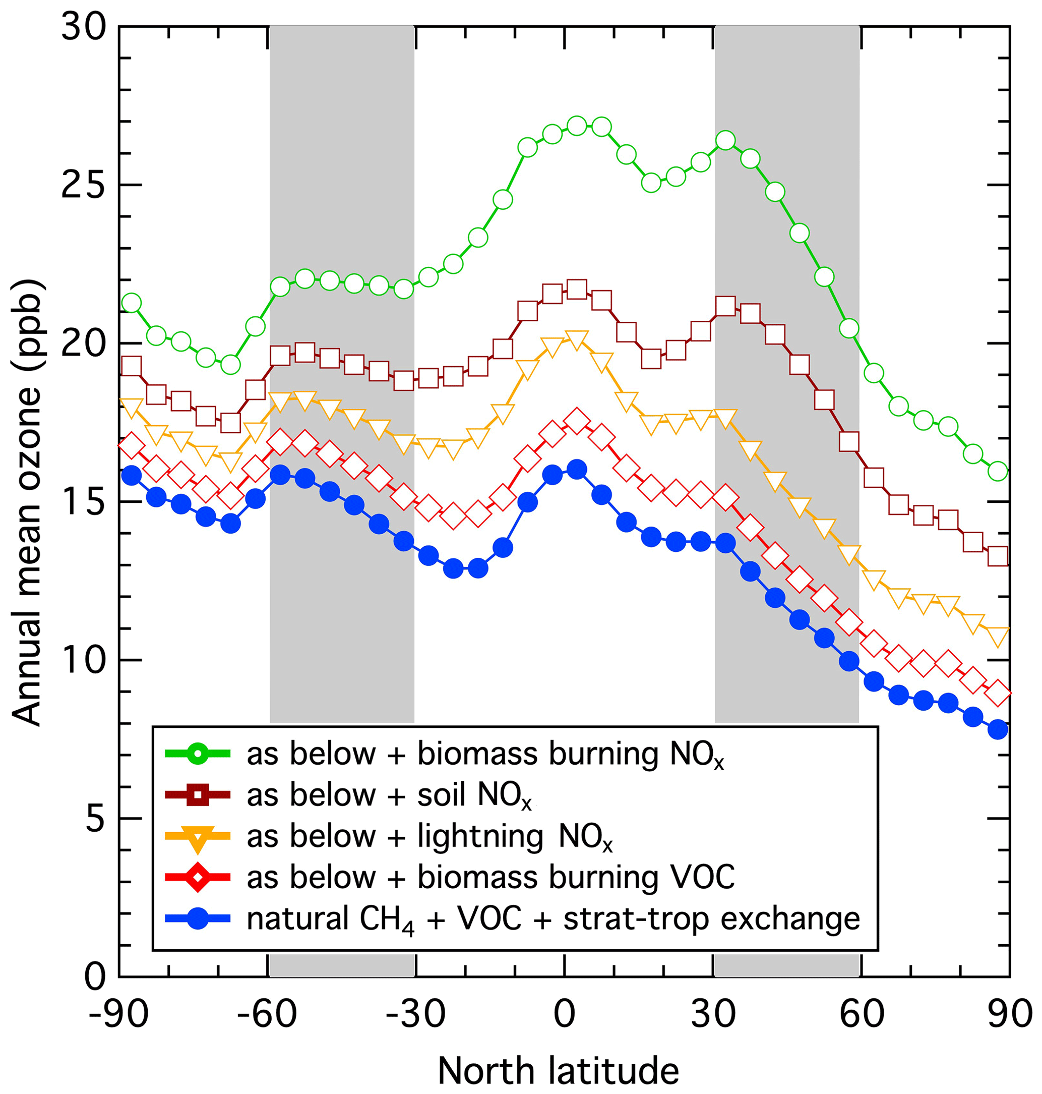
Figure 1 Pre-industrial latitude dependence of zonal surface annual mean ozone mixing ratios calculated by the STOCHEM-CRI for progressively larger assumed NO_x emission scenarios. The base case assumes a pre-industrial methane mixing ratio of 718 ppb, together with 506 Tg yr⁻¹ isoprene and 126 Tg yr⁻¹ terpene emissions. The shaded regions indicate midlatitudes. The assumed natural NO_x emissions are 0.6 Tg N yr⁻¹ for stratosphere–troposphere exchange, 5.0 Tg N yr⁻¹ for lightning, 5.6 Tg N yr⁻¹ for soils and 6.8 Tg N yr⁻¹ for biomass burning.

Global atmospheric chemistry model simulations indicate that a reversal of the interhemispheric ozone gradient is plausible. Wang and Jacob (1998) used a global three-dimensional model of tropospheric chemistry to investigate pre-industrial ozone levels and discussed uncertainties and potential difficulties. Of particular importance was the level of the pre-industrial NO_x emissions. Figure 1 examines the dependence of the interhemispheric ozone gradient upon the assumed magnitude of the natural NO_x emissions through five simulations of the global Lagrangian chemistry-transport model (STOCHEM-CRI). The base case assumes no NO_x emissions to the troposphere; under these conditions photochemical ozone production is small, with the required NO_x precursor provided only by formation from nitric acid entering the troposphere through stratosphere–troposphere exchange. A reversed ozone gradient arises from the faster surface deposition of ozone to land surfaces in the Northern Hemisphere. Biomass burning emissions in the second simulation contain a wide range of trace gases, but with NO_x emissions excluded, ozone levels increase somewhat but the reversed gradient is not significantly affected. As pre-industrial NO_x emissions (from lightning, soil emissions, and biomass burning) are added step-wise (third through fifth simulations), ozone levels rise and the reversed gradient is gradually eroded at midlatitudes.

Comparisons of observed ozone concentrations with simulations by modern global atmospheric chemistry models provide useful tests of the models and hopefully useful guidance for their improvement. One fruitful comparison arises from analysis of measurement records to establish, as accurately as possible, the long-term ozone changes that occurred in the background troposphere as industrial development proceeded, particularly at northern midlatitudes. Challenges for this analysis include the sparseness of the measurement record and uncertainty regarding the accuracy of measurements made by different researchers using a variety of techniques at different locations. The Task Force of Hemispheric Transport of Air Pollutants (HTAP, 2010; Parrish et al., 2012, 2014) quantified long-term ozone changes at northern midlatitude sites, predominately in Europe. As part of the Tropospheric Ozone Assessment Report (https://igacproject.org/activities/TOAR, last access: 28 February 2021), Tarasick et al. (2019) critically reviewed the record of historical ozone measurements throughout the global troposphere. Parrish et al. (2021a) have recently synthesized the HTAP and TOAR analyses. A second goal of this work is to compare these observational analyses with results from recent Earth system model (ESM) simulations.

In this work, the interhemispheric comparison of long-term tropospheric ozone changes is limited to the MBL, since the available measurements from the SH were all collected in the MBL; there are no higher elevation SH sites with extensive records. Nevertheless, long-term changes of ozone in the MBL do reflect the concurrent changes in the free troposphere, because entrainment of ozone from the free troposphere is the primary source of ozone to the MBL. Parrish et al. (2012, 2014, 2020) demonstrate that long-term ozone changes are similar from the surface to the mid-troposphere based upon comparisons of observed concentrations at baseline-representative sites in the MBL, at mountain top sites, and in the free troposphere from balloon-borne sondes and aircraft.

High-quality measurements from two MBL sites – Cape Grim, Australia, in the SH and Mace Head, Ireland, in the NH – provide the primary basis for our analysis. These measurements extend from the 1980s to the present and are representative of baseline conditions in the troposphere. By baseline conditions, we mean measurements collected during periods when air is transported to the measurement site from the marine environment, thereby avoiding confounding influences from nearby continental areas – see discussion in chap. 1 of HTAP (2010). Two different strategies are employed to extend each of these ozone records back to 1950. Before the 1970s, limited MBL measurements are also available from other sites in both hemispheres that provide support for the ozone changes derived for the 1950 to 1980 period. These measurements were conducted at coastal sites relatively isolated from nearby influences, so they are expected to be directly comparable to the two primary data sets. Post-1980 data from other MBL sites in both hemispheres provide comparisons for the more recent Cape Grim and Mace Head data.

2 Methods

The analysis in this paper is based on the results of published observational and model simulation studies that allow quantification of long-term ozone changes from 1950 to the present in the MBL at midlatitudes in both hemispheres. No continuous ozone measurement record covering the entire period from pre-industrialization to the present exists in either hemisphere; thus, we use less direct approaches to construct long-term ozone records from the available observations. Herein we discuss linear and polynomial fits to time series of ozone measurements; these fits with associated confidence limits are derived from standard least-squares fitting procedures, such as discussed in chap. 6 and 7 of Bevington and Robinson (2003). All fits were performed with the WaveMetrics IGOR Pro software package. Ozone concentrations are consistently expressed as mole fractions (i.e., mixing ratios) in units of nmol O₃/mole air (referred to as ppb). Quantitative results are given with indicated uncertainties, which are 95 % confidence limits unless stated otherwise.

The analysis presented here is based on MBL ozone observations that fall into two categories: recent (1982 to 2017) continuous measurements and older (1956 to 1984) measurements made over limited time periods. Table 1 gives the locations, elevation, and years of measurements for these data sets. The primary analysis is based on the continuous, recent measurements from Mace Head and Cape Grim. The Mace Head data are those selected as representative of the unpolluted NH MBL (i.e., baseline conditions) as discussed by Derwent et al. (2018a); Table 1 in Appendix A of their Supplementary Data gives the monthly means, which are considered here. The annual mean Cape Grim data were downloaded from the TOAR data archive (Schultz et al., 2017; https://join.fz-juelich.de/access/, last access: 20 April 2020); they were not selected for baseline conditions. Parrish et al. (2020) discuss a time series of baseline selected, seasonal mean ozone mixing ratios derived from measurements at sites in the Pacific MBL at the US west coast; these data provide a comparison for the Mace Head data. The US Pacific MBL monthly mean data are given in Table S1 of the Supplement. For the analysis here, annual means at Mace Head and the US Pacific MBL are derived from the tabulated monthly means for each year with all 12 months of data available. Data from all times of day are included for the Cape Grim, Mace Head and US Pacific MBL data sets.

Table 1 Ozone data sets and analyses utilized in this work.

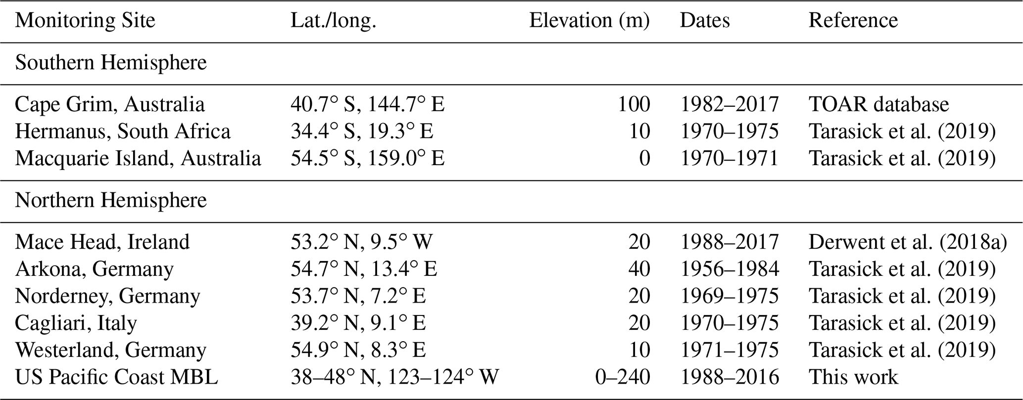
The older measurements are multi-year means taken from Tarasick et al. (2019). We utilize the results accepted into their record (their Tables 4 and 6) from midlatitude MBL sites (included in Table 1) in both hemispheres. In figures showing the results, the mean of the measurements made over multiple years are plotted at the center of the measurement period. Tarasick et al. (2019) conclude that some of these results are of questionable reliability, a conclusion that is considered in the discussion of these data. The TOAR effort did not attempt baseline filtering for these ozone records, so any impact of local or regional pollution-related influences remains unquantified.

The measurement programs providing the two primary data sets were initiated too late (1982 and 1988 at Cape Grim and Mace Head, respectively) to directly characterize ozone changes from 1950 to the present. Southern midlatitude long-term ozone changes have been small (e.g., Cooper et al., 2014; Tarasick et al., 2019), so a standard linear regression fit to the Cape Grim annual means extrapolated back to 1950 is a suitable method to derive an ozone trend over the entire period; Table 2 gives the parameters of this fit. Long-term ozone changes at northern midlatitudes have been much larger than in the SH (e.g., Cooper et al., 2014), so a simple extrapolation approach is not appropriate; here we quantify the long-term ozone change at Mace Head from the analysis developed during the HTAP study (HTAP, 2010; Parrish et al., 2012, 2014).

The HTAP analysis followed the suggestion of Crutzen (1988): “it would be very interesting to compare certified old data with modern data taken at the same sites as where the `ancient' data were taken.” The “ancient” data considered are the sparse record of early measurements made at baseline representative sites throughout Europe, which extend back to 1950, with two summer measurement periods from the 1930s. Tarasick et al. (2019) “certified” the “ancient data” to the extent possible by carefully evaluating the early measurements; these results were compared to modern data collected at those same sites. The long-term ozone change quantification is based on relative ozone changes, which are derived by dividing each time series of seasonal means at each measurement site by the year 2000 intercept of a fit to those means. Parrish et al. (2014) found that the relative long-term changes are the same within statistical confidence limits at all baseline-representative European sites, but with some seasonal differences. Later analysis (Parrish et al., 2020) showed that those seasonal differences are not significant and that the relative long-term ozone changes are the same, within statistical confidence limits, for all seasons. Figure 2a shows the 757 relative seasonal means available from all seasons at six baseline-representative European sites. Even though the relative ozone concentrations have substantial scatter, the large number of data allow precise polynomial fits to the overall time series. The fits included in Fig. 2a are a linear regression over 1950 to 2000, a cubic (i.e., third-order) polynomial over 1950 to 2010, and a fourth-order polynomial over 1934–2010. The three fits give similar changes over the 1950 to 2000 period: factors of 2.23, 2.16 and 2.08 for the linear, cubic and fourth-order polynomial fits respectively. Each of these three factors agrees with the 1950 to 2000 relative change of 2.1 ± 0.2 derived in a synthesis of the HTAP and TOAR analyses (Parrish et al., 2021a). Parrish et al. (2014) also show that simulations by three CMIP5 global chemistry climate models agree that relative means in all seasons at all European baseline-representative sites exhibit similar relative long-term changes; simulations from one model are shown in Fig. 2b and from the other two models in Fig. S1. Figures S1–S8 of Parrish et al. (2014) illustrate the normalization process and analysis for these same measurement and model results for separate seasons. Figure 2 indicates that to estimate the long-term ozone change at Mace Head (or any other baseline representative site in western Europe) over the 1950 to 2010 period for which measurements are available, one needs only to quantify the year 2000 mean ozone at the site and then calculate the product of that intercept with the polynomial fit.

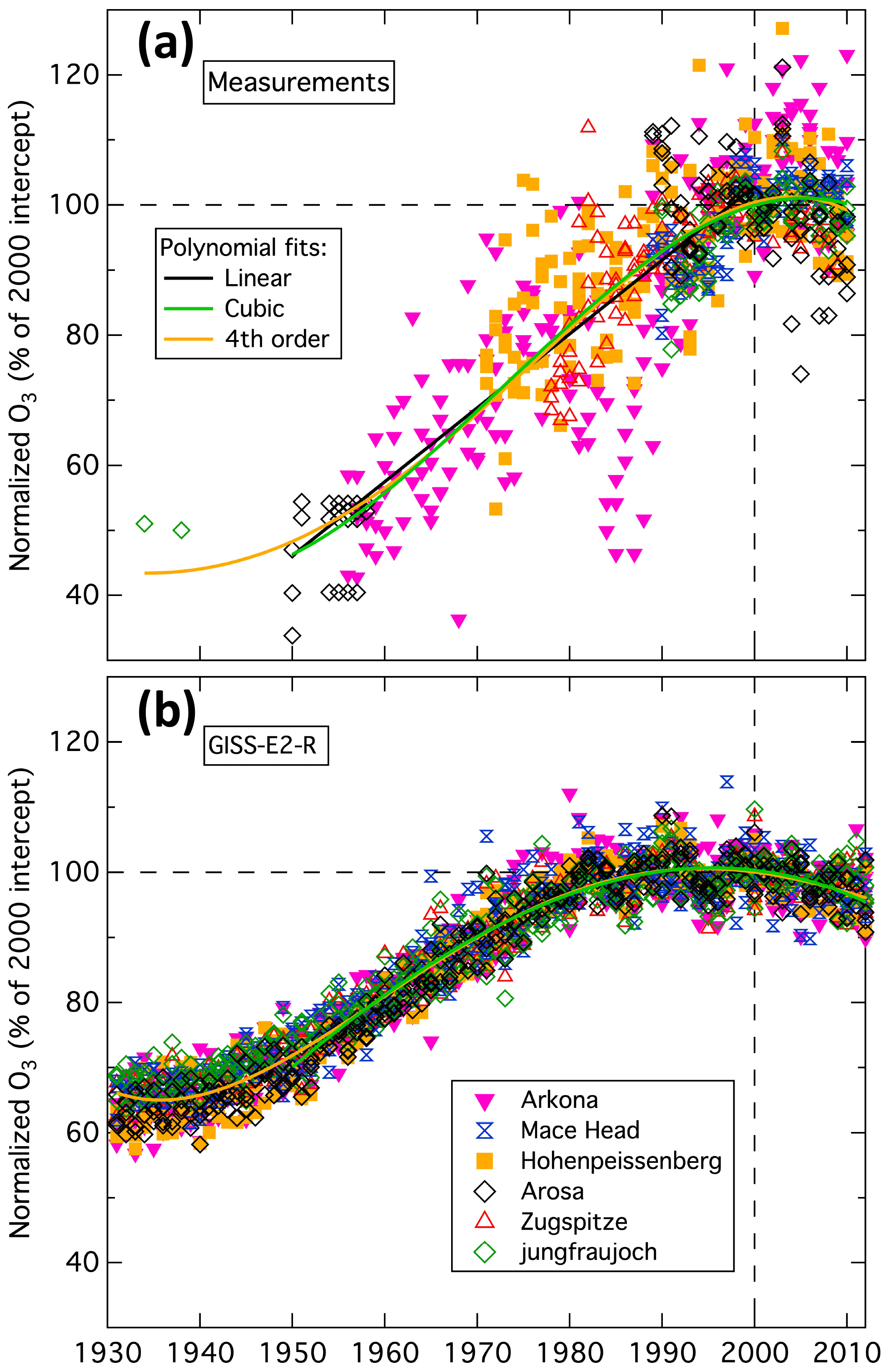
Figure 2 Normalized, seasonal mean ozone measured (a) and simulated (b) at the six baseline representative European sites considered by Parrish et al. (2014). The simulations are from the GISS-E2-R model. Each graph includes cubic (beginning in 1950 – green curve) and fourth-order polynomial (gold curve) fits to all seasonal means; (a) also includes a linear fit (1950–2000 – black line).

The HTAP-based analysis approach utilized here relies on the concept that baseline ozone concentrations followed the same relative long-term changes throughout northern midlatitudes. Simple transport and ozone lifetime considerations support this picture; in the free troposphere at northern midlatitudes the net lifetime of ozone is estimated as 100 d, which is considerably longer than either the circum-global transport time (∼ 30 d) or the vertical overturning timescale (∼ 20 d). Consequently, even though the many sources and sinks of ozone are heterogeneously distributed, and each can possibly change differently over long timescales, the relatively rapid mixing and transport ensure that those changes are all reflected in approximately constant average baseline ozone concentration changes throughout northern midlatitudes. In the presence of relatively rapid transport and mixing, there simply is no mechanism that can maintain heterogeneity in the long-term changes in the zonal baseline ozone concentrations. Parrish et al. (2020, 2021b) discuss these considerations in greater detail.

The European historical ozone data considered by Parrish et al. (2014) and included in Fig. 2a lacked quantified uncertainties. However, the accuracy of relative long-term ozone changes derived from these data is supported by the critical evaluation of Tarasick et al. (2019), which found no significant, systematic inaccuracy in the historical data analyzed by Parrish et al. (2012, 2014). Parrish et al. (2021a; their Fig. 1) show that the seasonal and annual mean long-term changes derived as described above provide good fits to all of the historical European data identified by Tarasick et al. (2019). The observations in Fig. 2a do show substantial scatter about the fits, with a root-mean-square deviation (RMSD) of 8.9 % of the year 2000 intercept for the cubic fit. To be representative of the historical data, this RMSD must be referenced to the smaller magnitude of the historical data; the corresponding RMSD is then ∼ 16 % when referenced to the year 1960 intercept. Tarasick et al. (2019) estimate a relative uncertainty of 0.7–1.2 at approximately 90 % confidence intervals for the methods employed to collect the historical data; this corresponds to a relative standard deviation of ∼ 15 %, assuming a normal distribution of measurement errors. Thus, the historical data included in Fig. 2a are judged to be as accurate and precise as can be expected from the historical measurement methods.

The model results that we compare to the measurements are from three sources: six ESMs (identified in Figs. S2 and S3) that took part in the CMIP6 exercise, three chemical-climate models (CCMs) (identified in Fig. S4) that took part in the CMIP5 exercise, and the STOCHEM-CRI model described by Derwent et al. (2018b). Table S2 references descriptions of the CMIP6 ESMs, and Parrish et al. (2014) give more details and references for the simulation results of the CMIP5 CCMs. Surface concentrations of ozone at Mace Head and Cape Grim were obtained from the six CMIP6 models that had made data available on the Earth System Grid Federation (ESGF) at the time of writing. Ozone concentrations were also obtained from these same models for the model level that included the site elevation for eight additional NH and two additional SH baseline sites. All ESM results are from the coupled historical simulations over the 1850 to 2014 period from all available ensemble members of each CMIP6 model. STOCHEM-CRI is a global Lagrangian chemistry-transport model with a detailed description of tropospheric chemistry which makes it suitable for studies of low NO_x and isoprene chemistry (Jenkin et al., 2019) and the pre-industrial atmosphere (Khan et al., 2015). STOCHEM-CRI is driven by meteorological fields from the UK Meteorological Office Unified Model taken from an archive for 1998, further details of which are given in Collins et al. (1997); ozone sources in this model are dominated by stratosphere–troposphere exchange, which was set to 745 Tg O₃ yr⁻¹. The Condensed Reactive Intermediates (CRI) mechanism is a condensed version of the highly detailed and explicit Master Chemical Mechanism (MCM) v3.3.1 (http://mcm.york.ac.uk/home.htt, last access: 23 June 2021). Both rely entirely on evaluated laboratory chemical kinetics studies for their rate coefficient and product yield data, which is important in the present context of the pre-industrial atmosphere because low NO_x conditions are not accessible in the smog chamber studies that have been an important source of mechanistic data for the chemistry of polluted atmospheres. Derwent et al. (2021) document the fidelity of the MCM and CRI mechanisms in a chemical mechanism intercomparison focused on the low NO_x conditions of the pre-industrial troposphere.

3 Results

The sparse records of available baseline ozone measurements made in the midlatitude MBL of both hemispheres are compared in Fig. 3. The symbols after 1980 are annual means of baseline-selected data from three representative long-term measurement records – Cape Grim in the SH and Mace Head and the US Pacific MBL in the NH. The seven symbols before 1980, two in the SH and five in the NH, represent relatively short (2 to 16 years), year-round records evaluated in TOAR (Tarasick et al., 2019). The map in Fig. 3 identifies the site locations, and Table 1 gives site and data record information. We quantify the MBL baseline ozone mixing ratios as accurately as these limited data allow, in order to compare long-term changes between the two hemispheres.

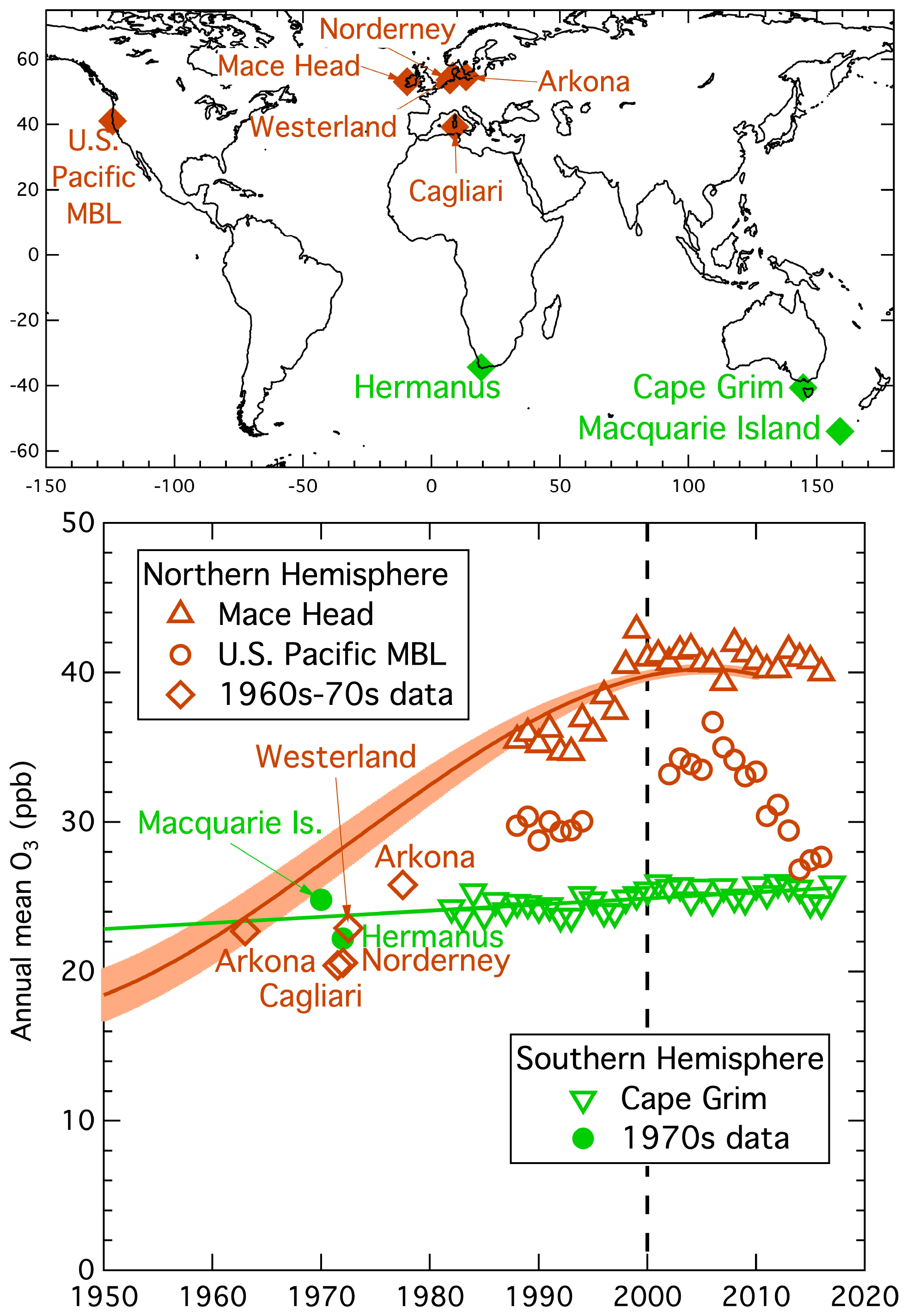
Figure 3 Long-term changes in annual mean baseline ozone mixing ratios measured at midlatitude, low-elevation coastal sites indicated on the map in the Northern Hemisphere (brown symbols) and Southern Hemisphere (green symbols). The symbols for the longer-term, more recent data sets (Mace Head and Cape Grim) represent individual annual means; the symbols for the data from the 1960s and 1970s (Tarasick et al., 2019) represent averages over the variable periods (see Table 1) of available data. The derivation of the brown solid curve is described in the text; the shaded area about the curve indicates estimated confidence limits for the curve. The green solid line is a standard linear regression to the Cape Grim data, with extrapolation back to 1950.

The year 2000 annual mean mixing ratios at Mace Head and the US Pacific MBL are 39.8 ± 0.6 and 32.9 ± 1.1 ppb, respectively (Parrish et al., 2020). The difference in these annual means represents significant zonal variation in MBL ozone concentrations between the eastern North Pacific and eastern North Atlantic oceans. Since the NH MBL data reported by Tarasick et al. (2019) are all from European measurements, we will primarily focus on the Mace Head data in this analysis. The Mace Head measurements agree closely with other North Atlantic MBL sites; year 2000 annual mean mixing ratios are 38.5 ± 0.5 and 37.3 ± 1.3 ppb at Storhofdi, Iceland, and Tudor Hill, Bermuda, respectively (Parrish et al., 2016). The long-term trends derived for the two representative NH sites before 2010 (i.e., beginning in 1988) are consistent with each other: 0.31 ± 0.10 ppb yr⁻¹ at Mace Head and 0.27 ± 0.08 ppb yr⁻¹ at the US Pacific MBL (Cooper et al., 2014).

Measurements at Cape Grim extend back to 1982. These data agree closely with those at two other southern midlatitude MBL sites – year 2000 annual mean mixing ratios of 25.0 ± 0.2 ppb at Cape Grim compared to 23.1 ± 0.4 and 23.7 ± 0.4 ppb at Cape Point, South Africa, and Ushuaia, Argentina, respectively; these three sites also have similar seasonal cycles (Parrish et al., 2016). These results from three continents demonstrate the zonal similarity of tropospheric ozone concentrations at southern midlatitudes. Thus, we take the Cape Grim data record to be representative of the entire southern midlatitude MBL. The solid green line in Fig. 2 indicates the linear fit over the entire data record, with a small, but statistically significant, long-term trend of 0.041 ± 0.019 ppb yr⁻¹, which is a factor of ∼ 7 smaller than at the two NH sites. To guide the discussion of changes that may have occurred before the beginning of these measurements, this linear fit is extrapolated back to 1950, giving an estimate of the mean concentration in that year of value. This extrapolation may overestimate the earlier changes, as it is not known when the increase began. However, this trend is small enough that this uncertainty has negligible impact on the following discussion.

As is apparent from Fig. 3, no single site measurement record covers the complete 1950 to 2010 period or includes annual means before 1950 at northern midlatitudes. However, the quantification of the common relative long-term ozone change over western Europe from all available baseline sites (Fig. 2) allows estimation of the long-term ozone change at Mace Head for that period; the cubic fit (green curve) illustrated in Fig. 2 multiplied by the Mace Head year 2000 mean ozone (given above) yields the brown polynomial curve in Fig. 3 (coefficient values given in Table 2). The long-term changes in ozone derived for Mace Head are given by that curve with the shading indicating the confidence limits derived from the propagation of the confidence limits of the Mace Head year 2000 mean and the overall relative increase of baseline ozone over Europe of a factor of 2.1 ± 0.2 (Parrish et al., 2021a). Notably, Tarasick et al. (2019) conclude that baseline ozone increased in the NH by a smaller amount (30 %–70 %, with large uncertainty) between the period of historic and present-day observations; however Parrish et al. (2021a) show that their comparison of historic data (collected at a set of primarily baseline representative sites at coastal and mountain locations) with modern data, collected at rural, low-elevation sites within the European continental boundary layer, introduced several biases into their comparison, all of which caused systematic underestimates in their derived differences between the historic and modern data. Parrish et al. (2021a) discuss these biases in detail and give estimates of their magnitudes, which are large enough to account for this apparent disagreement.

Table 2 Coefficients of polynomials ($a+bt+c{t}^{\mathrm{2}}+d{t}^{\mathrm{3}}$, where t= year − 2000) that define the long-term ozone changes given by the cubic polynomial fit in Fig. 2a and the solid curves in Figs. 3 and 4.

^* % unit indicates percentage of year 2000 intercept of annual means.

The means of the older (1960–1980) data included Fig. 3 do not differ significantly between the two hemispheres; they are 23.5 ± 1.8 and 22.5 ± 2.2 ppb (where standard deviations are indicated) for the two SH and five NH data sets, respectively. These limited data indicate that the large interhemispheric gradient apparent in today's measurements was not present in the 1960–1980 period. Figure 3 shows that the extrapolation of the Cape Grim data agrees closely with the SH data from Macquarie Island and Hermanus, in accord with the small trends and zonal similarity of tropospheric ozone concentrations at southern midlatitudes. The mean of the five NH points, all from European measurements, is smaller than the 27.2 ppb value of the brown curve in 1970, and this curve is above all of the pre-1980 MBL measurements as well as the more recent US Pacific MBL data; this indicates that this curve, derived for Mace Head, provides an upper limit for NH midlatitude baseline ozone in the MBL. It should be noted that Tarasick et al. (2019) judge four (Norderney, Cagliari, Westerland and Hermanus) of these seven earlier data sets to be of questionable reliability; however, exclusion of these data does not significantly change the overall agreement of the 1960–1980 data with the derived changes in either the NH or SH.

4 Discussion and conclusions

The ozone measurements illustrated in Fig. 3 lead to the conclusion that tropospheric ozone concentrations likely were higher in the SH than the NH before industrial development. Three lines of reasoning support this deduction. First, the sparse measurement record at baseline sites indicates that between 1950 and 2000 ozone concentrations increased by a factor of 2.1 ± 0.2 in the NH (Fig. 2 and Parrish et al., 2021a) and a factor of 1.09 ± 0.04 in the SH (Cape Grim fit in Fig. 3), which would imply an approximate doubling (factor of 1.93 ± 0.20); however present NH ozone concentrations are less than a factor of 2 greater than those in the SH (factor of 1.60 ± 0.03, based on year 2000 Mace Head to Cape Grim ratio), indicating that ozone concentrations likely were lower in the NH than the SH in 1950. Second, the brown and green curves in Fig. 3 intersect in about 1962, indicating that the NH ozone concentrations likely were lower than those in the SH in earlier years. Third, that curve intersection indicates that the MBL ozone concentrations were similar in both hemispheres in the 1960s, and the few available measurements from that period are all consistent with that similarity; however, multiple considerations indicate that anthropogenic precursor emissions had already substantially increased NH ozone concentrations by that time. By 1962 the brown curve in Fig. 3 had increased by ∼ 20 % from 1950 levels, and global model calculations (see discussion below) also find that NH ozone concentrations had increased significantly before the 1960s. Further, extremely elevated ozone concentrations (several 100 ppb) were observed in Los Angeles as early as the 1950s (Haagen-Smit, 1954). The emissions responsible for those urban ozone enhancements were primarily from on-road vehicles, which were common to all US urban areas. Those US emissions, and similar emissions in other countries at northern midlatitudes, are expected to have impacts throughout the NH midlatitude troposphere. Thus, although the measurement record is sparse, observations and the wider considerations discussed above are all consistent with the conclusion that in the pre-industrial troposphere, midlatitude ozone concentrations were higher in the SH than the NH. The cause of the greater increases in the NH and likely reversal of the natural interhemispheric ozone gradient is attributed to the increased emissions of ozone precursors that accompanied industrial development, and those increased emissions were predominantly located in the NH.

Differences in ozone sinks and/or sources between hemispheres can account for larger natural ozone concentrations in the SH compared to the NH. The loss rate of ozone to ocean surfaces is slow, but it is much faster over continents due to surface deposition to vegetation and to reaction with natural hydrocarbons emitted from forests. The fractional coverage of midlatitudes by land is ∼ 50 % in the NH, but only 6 % to 7 % in the SH, implying significantly slower ozone losses in that hemisphere. Molecular hydrogen may provide an analogy to ozone. Its average concentration is higher in the SH (Simmonds et al., 2000); this distribution is attributed to greater uptake by soils in the NH, despite there being active photochemical sources and sinks of hydrogen in both hemispheres and evidence for significant anthropogenic pollution sources concentrated in the NH. However, for hydrogen the greater NH pollution source is not large enough to reverse the natural interhemispheric gradient of hydrogen.

Comparisons between observations and global model simulations provide a basis to elucidate the causes of the changing interhemispheric ozone gradient, as well as to assess model performance. Figure 4 compares the observational-derived long-term changes from Fig. 3 with time series of annual mean surface ozone at Mace Head and Cape Grim simulated by six ESMs that participated in the sixth Coupled Model Intercomparison Project (CMIP6; Eyring et al., 2016). Figure S2 shows those same model simulations for the entire 1850–2014 simulation period with each of the six models identified. In Fig. 4 the simulated concentrations in recent years (after ∼ 1990) all agree within ∼ 5 ppb with the observations in both hemispheres. Section S1 of the Supplement gives further discussion of this agreement at 10 NH and 3 SH baseline sites, and includes comparisons with simulations by three CMIP5 models.

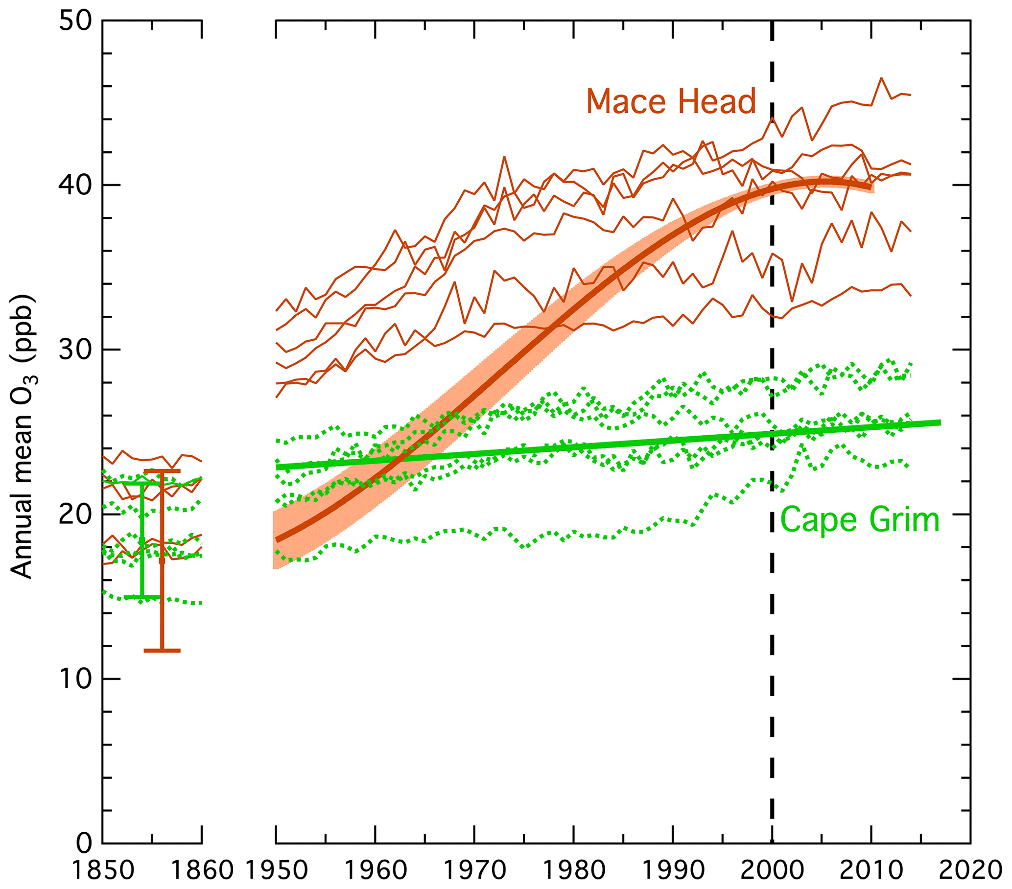
Figure 4 Comparison of modeled and measured long-term changes in annual mean ozone mixing ratios at Mace Head and Cape Grim from 1850–1860 (left) and after 1950 (right). The fits to the measurements (heavy solid line and curve on the right) are the same as those in Fig. 3. The thinner solid (for Mace Head) and dotted (for Cape Grim) curves are results from six ESMs that participated in the CMIP6 exercise. The two symbols on the left show the range of annual mean pre-industrial midlatitude (30^∘ to 60^∘) surface ozone calculated by the STOCHEM-CRI model for the five simulations discussed in the text.

The ESM simulations generally agree that long-term changes in SH ozone have been small, but they do not reproduce the rapid increase in ozone that occurred in the NH between 1950 and 2000. At Cape Grim the mean model trend over the 1982–2014 period of observations is 0.082 ppb yr⁻¹, with model results varying from 0 to 4 times the observed trend of 0.041 ± 0.019 ppb yr⁻¹. In a comparison of simulations by four of these same ESMs, Griffiths et al. (2021) found similarly good agreement at Cape Grim, as well as three other remote background sites, but did not compare those simulations with any northern midlatitude observations. The modeled 1950 to 2000 increases at northern midlatitudes correspond to a mean factor of 1.3 with a standard deviation of 0.1, while observations indicate a 2.1 ± 0.2 factor increase. It is notable that the overall modeled northern midlatitude ozone increase since pre-industrial times is a factor of 1.9 with a standard deviation of 0.3, as judged from the mean model ratio over the entire 1850 to 2000 period; this value agrees more closely with the observed 1950 to 2000 ratio of 2.1 ± 0.2, which we interpret as a good approximation for the factor of total ozone increase during northern midlatitude industrialization. This closer agreement is in accord with the analysis of Staehelin et al. (2017) that also found smaller model-simulated ozone increases at northern midlatitudes over the post-1950 period. They suggest that this discrepancy may be attributable to problems in quantifying changes in the historical emissions of ozone precursors from anthropogenic sources, and they discuss evidence for a significant impact from such problems.

The ESMs also do not simulate lower pre-industrial midlatitude ozone in the NH; the 1850 mean NH $/$ SH ratio is 1.13 with a standard deviation of 0.11, with only one of the six ESMs finding a ratio (slightly) less than unity. The full range of the five pre-industrial STOCHEM-CRI scenarios (with natural NO_x emissions between 0.5 and 18 Tg N yr⁻¹) from Fig. 1 is also indicated in Fig. 4; the scenarios that gave the largest ozone concentrations, i.e., those with the largest pre-industrial NO_x emissions, generally agree with the ESM simulations, but those with lower NO_x emissions give lower ozone concentrations with SH ozone higher than NH ozone. The absence of a reversed ozone gradient in the ESM simulations may indicate that the assumed natural NO_x emissions are too large. For reference, the natural NO_x emissions assumed in three of the six ESMs considered here are ∼ 11 to 14 Tg N yr⁻¹ (Fig. 1 of Griffiths et al., 2021), which are near the larger of the pre-industrial STOCHEM-CRI scenarios. If the natural NO_x emissions are too large, then the model-calculated radiative forcing of ozone is too small.

Other processes that affect ozone also differ significantly between hemispheres; thus, uncertainties in their parametrizations may also contribute to ESMs simulating higher pre-industrial ozone in the NH. Stratosphere–troposphere exchange (STE) is an important natural ozone source. A recent review of the tropospheric ozone budget (Archibald et al., 2020) suggests that the stronger Brewer–Dobson circulation in the NH produces a larger STE ozone flux in that hemisphere (∼ 57 % of total). However, Škerlak, et al. (2015) find that deep tropopause folds, which are most efficient for transporting stratospheric ozone into the lower troposphere, are more frequent in the SH. The absolute and relative magnitudes of ozone loss to land and ocean surfaces differ strongly between hemispheres. Luhar et al. (2018) give a new parameterization scheme that reduces deposition to oceanic surfaces by a factor of ∼ 3 compared to earlier work; incorporation of this new result into ESMs would raise SH ozone relative to the NH. The surface deposition of ozone to land surfaces occurs predominately in the NH, and its representation in current models is regarded as insufficient (Clifton et al., 2020). Another concern is the model treatment of the chemistry of natural hydrocarbons (e.g., isoprene and terpenes) emitted in large quantities from temperate forests that are predominately located in the NH. At the low NO_x concentrations believed to have dominated the pre-industrial continental boundary layer, this chemistry constitutes an important ozone sink, while at the higher modern-day NO_x concentrations, it is an ozone source. Understanding the NO_x concentration dependence of this complex natural hydrocarbon chemistry is still an active area of research (e.g., Jenkin et al., 2015). The magnitude of the pre-industrial emissions of these natural hydrocarbons is also quite uncertain (Mickley et al., 2001), and the CMIP6 models use a variety of estimation approaches.

In addition to the above-discussed model uncertainties that most directly affect the ozone gradient, Wild et al. (2020) identify key areas in model simulations that require improvement for accurate simulation of the tropospheric ozone distribution; these include the atmospheric water vapor distribution and the drivers of variability in global OH, which differ significantly between models. Derwent et al. (2021) identify key improvements required in the representation of the atmospheric chemistry of the pre-industrial troposphere in ESMs and other global chemistry-transport models. Additional improvements to the treatment of the atmospheric chemistry of natural and anthropogenic ozone precursors, especially NO_x, and of ozone loss processes are likely required to accurately treat the balance of ozone production and loss in both the present-day and pre-industrial troposphere, a requirement necessary to accurately model the interhemispheric ozone gradient and fully understand the radiative forcing of tropospheric ozone.