the Creative Commons Attribution 4.0 License.
the Creative Commons Attribution 4.0 License.
 | 28 Jun 2021
Identifying meteorological influences on marine low-cloud mesoscale morphology using satellite classifications
Robert Wood
Tianle Yuan
Ryan Eastman
Lazaros Oreopoulos
Marine low-cloud mesoscale morphology in the southeastern Pacific Ocean is analyzed using a large dataset of classifications spanning 3 years generated by machine learning methods. Meteorological variables and cloud properties are composited by the mesoscale cloud type of the classification, showing distinct meteorological regimes of marine low-cloud organization from the tropics to the midlatitudes. The presentation of mesoscale cellular convection, with respect to geographic distribution, boundary layer structure, and large-scale environmental conditions, agrees with prior knowledge. Two tropical and subtropical cumuliform boundary layer regimes, suppressed cumulus and clustered cumulus, are studied in detail. The patterns in precipitation, circulation, column water vapor, and cloudiness are consistent with the representation of marine shallow mesoscale convective self-aggregation by large eddy simulations of the boundary layer. Although they occur under similar large-scale conditions, the suppressed and clustered low-cloud types are found to be well separated by variables associated with low-level mesoscale circulation, with surface wind divergence being the clearest discriminator between them, regardless of whether reanalysis or satellite observations are used. Clustered regimes are associated with surface convergence, while suppressed regimes are associated with surface divergence.
- Article
(2474 KB) - Full-text XML
- BibTeX
- EndNote


Marine low clouds are radiatively important, with a strong cooling effect on the planet. They also display a wide range of morphologies, which have differing radiative properties (Chen et al., 2000). Classically, ship-based observations have classified marine low clouds using the familiar World Meteorological Organization (WMO) cloud types such as stratocumulus (Sc), cumulus (Cu), etc. (e.g., Warren et al., 1988). However, clouds also form larger mesoscale, morphologically distinct organizations that would not be apparent from the limited perspective of a surface-based observer. These mesoscale cloud patterns are of particular interest for several reasons. First, they have been shown to represent different underlying marine boundary layer (MBL) regimes (e.g., Wood and Hartmann, 2006; hereafter WH06), namely the influence of an additional environmental MBL property that covaries with cloud morphology. Second, prior work has shown that the mesoscale organization regulates the relationship between albedo and cloud fraction (CF; McCoy et al., 2017). Third, larger mesoscale patterns are clearly visible from current-generation satellite imagers, allowing for their classification using computer image recognition and subsequent generation of a potentially informative MBL cloud dataset on a near-global and highly temporally resolved scale for studying these clouds and their drivers.
In the midlatitude storm tracks and eastern ocean subtropical Sc decks, stratiform low-cloud types dominate (Hartmann et al., 1992). These high-cloud-fraction cloud types are particularly effective coolers, and as a result their organization and structure have been the subject of extensive investigation (Agee, 1987; Muhlbauer et al., 2014). In lower latitudes and away from the eastern subtropical ocean basins, Sc clouds are rarer, and instead we often find boundary layers (BLs) dominated by cumuliform cloud types, sometimes clustering into large convectively active regions and some other times in relatively isolated smaller Cu. Figure 1, adapted from an observation-based climatic cloud atlas (Hahn and Warren, 2007), shows the difference between the frequency of occurrence of Cu clouds and that of Sc clouds; the commonly occurring “Cu-under-Sc” case is classified as Sc for consistency with the view from above (Hahn et al., 2001). Red values indicate more Cu and show that boundary layer clouds over the ocean between 30∘ N and S are more often cumuliform. Although the average cloud radiative effect (CRE) of these clouds is lower, their ubiquity combined with a high mesoscale variability in cloud fraction makes them an important target of study.

Figure 1Difference in relative frequency of occurrence of cumulus and stratocumulus cloud types per Hahn et al. (2001) definitions from ship-based observations. Red areas highlight Cu-dominated MBLs, while blue regions have more Sc cloud.
Cumuliform MBLs have been observed to contain mesoscale aggregates of shallow convection in a number of different forms (LeMone and Meitin, 1984; Nicholls and Young, 2007). Bretherton and Blossey (2017) (hereafter BB17) demonstrated how mesoscale aggregation of warm shallow Cu presents in large eddy simulation (LES). In their conceptual model, the shallow convective self-aggregation is driven by convection–circulation–humidity feedbacks. These result in cloudy regions of aggregated convection with a positive mesoscale column water vapor and moisture anomaly as well as a strong low-level circulation with lower-boundary-layer convergence, acting to further concentrate moisture into the moist columns. The difference between this and the conceptual model for deep-convective self-aggregation (e.g., Emanuel et al., 2014) is that the latter relies on radiative feedbacks, which are not necessary to produce shallow mesoscale aggregation. BB17 demonstrated that the presentation of shallow aggregation agrees with this conceptual model and suggested that further observational validation is warranted.
When classifying stratocumulus and cumulus clouds, a common form of mesoscale variability is mesoscale cellular convection (MCC) (Agee, 1987). This can take the form of open-cellular or closed-cellular MCC. WH06 used a neural network to classify low-cloud scenes from satellite observations over the eastern subtropical Pacific Ocean into four categories, based on MCC type or absence thereof: open, closed, and cellular but disorganized MCCs and no MCC present. The utility of these classification-based approaches is evident in their ability to show the controls on cloud morphology in cold air outbreaks (McCoy et al., 2017), characterize properties and occurrences of the underlying regimes (Muhlbauer et al., 2014), or discern whether mesoscale morphology is more strongly driven by internal mechanisms or by large-scale meteorology (WH06). However, a limitation of the WH06 classification scheme is its inability to discriminate between cloud morphologies over the warmer regions of the tropical trades, where MCC is less dominant. Additionally, the power-spectra- and Fourier-transform-based feature vectors used for classification were very sensitive to the presence of high cloud, necessitating the strict exclusion of many otherwise visually identifiable scenes. More recent investigations of low-latitude marine low-cloud mesoscale variability, agnostic to previously identified forms of organization, have been successful in identifying distinct morphological regimes, using machine learning to classify a large dataset of cloud images (Stevens et al., 2020).
In this work we continue the exploration of marine low-cloud morphology drivers and characteristics with the new classification scheme introduced by Yuan et al. (2020) that expanded on WH06. The new scheme focuses on discrimination between different cumulus-dominated cloud types, particularly in the tropical trade wind regions. The machine learning approach adopted to create this new dataset uses convolutional neural networks (CNNs) to permit the inclusion of some scenes with thin or small amounts of high cloud. Two cumuliform low-cloud morphological types were added, clustered convection and suppressed convection, to capture more cloud morphological variability in the tropics and subtropics. Following a brief description of the new classification scheme and observational datasets (Sect. 2), we present the physical characteristics of the resulting cloud types in Sect. 3. Specifically, we validate in that section whether the presentation of the two cumuliform cloud types is consistent with the model for mesoscale aggregation of shallow cumulus convection described by BB17. We conclude with a discussion of the importance of these results (Sect. 4).
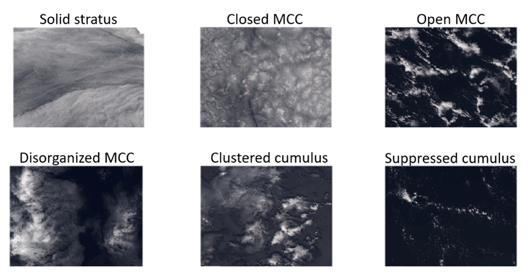
Figure 2Typical examples of scenes belonging to each of our classification categories. Image scale is roughly 100 km across. Images are captured using NASA Worldview.
We mainly perform composite analysis of various observational and model datasets by morphological cloud type. We first describe the cloud type classifications, then the datasets used, and finally the compositing methodology.
2.1 Cloud type classifications
The classification dataset used is derived from imagery by the Moderate-Resolution Imaging Spectrometer (MODIS), aboard the Aqua satellite. MODIS RGB visible imagery of 128 km×128 km (approximately ) cloudy scenes, filtered to remove scenes with >10 % coverage of high cloud, low cloud <5 %, and viewing angles >45∘, is manually classified as being comprised mostly of stratus cloud, closed-cellular marine cellular convective Sc (closed MCC), open-cellular Sc (open MCC), disorganized-cellular stratocumulus (disorganized MCC), clustered cumulus, or suppressed cumulus. These categories were chosen by examining the morphological climatologies in Muhlbauer et al. (2014), studying regions where there was little variability in morphology category (primarily the tropics, where disorganized MCC dominated), and identifying additional commonly occurring cloud morphologies. These (clustered and suppressed Cu) were then added to the pre-existing cloud categories, along with a homogeneous stratiform category initially used in Wood and Hartmann (2006). Examples of these types can be found in Fig. 2.
The scenes were then used to train a convolutional neural network (CNN) using as input the image of scene visible reflectance. A full description of the machine learning training and model evaluation can be found in Yuan et al. (2020). These authors found that average model precision evaluated on a test set was approximately 93 % across all categories. Open MCC had the lowest precision, most likely because it was the lowest-frequency category. The largest source of model confusion was between disorganized MCC and clustered Cu, which is unsurprising given the similar appearance of these categories. The primary difference between these two types is that disorganized MCC represents a regime with cellular convection at some characteristic scale, though not organized clearly into open- or closed-cell regimes, while clustered Cu represents aggregated convection at a variety of scales within a scene. When distinguishing between these two types during manual labeling, scene large-scale context proved helpful.
For this paper, most analysis is based on 3 years of CNN classifications from the southeast Pacific (SEP) region, (65∘ S–Equator, 140–40∘ W) which includes much of the Southern Ocean and a small portion of the southwest Atlantic, as well as classifications from summer 2015 in the northeast Pacific (NEP) region (Equator–60∘ N, 180–100∘ W) for co-location with aircraft data (see Sect. 3.5 below). The resulting tabular dataset contains location, time, and cloud scene classification as well as MODIS low-cloud fraction derived from the MODIS cloud product cloud top heights (MYD06; Platnick et al., 2017). Approximately 750 000 scenes were available for the SEP (averaging approximately 65 classifications per MODIS granule and 11 granules per day), while the NEP dataset is smaller, with ∼35 000 scenes. Relative distributions, normalized for each location, for the various cloud scene types are provided in Fig. 3. Due to geographical differences in cloud cover and satellite sampling, the number of viable scenes is not distributed evenly over the regions of interest, with approximately 5 times as many scenes in the subtropical Sc regions as in the midlatitudes.
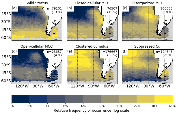
Figure 3Relative frequency of occurrence of each cloud type on a logarithmic scale. In the upper right corner of each panel, the total number of classifications over 3 years (2014–2016) as well as the total fraction of scenes of each type is shown. Gray areas are where fewer than 200 scenes are sampled.
2.2 Satellite-derived ancillary data
Surface wind divergence is derived from the Advanced SCATterometer (ASCAT) aboard MetOp-A, specifically the 0.25∘ gridded wind vectors (Ricciardulli and Wentz, 2016). For each classified scene, the co-located calculated ASCAT divergence values are extracted and averaged. Since the ASCAT swath width is much narrower than that of MODIS (even when filtering out high-viewing-angle scenes), many classified scenes (approximately 45 %) cannot be paired with wind data. Additionally, the overpass time of MetOp-A (∼ 09:30 LT – local time) does not coincide with Aqua (∼ 13:30 LT) so that any significant diurnal cycle in wind divergence could influence results. While this is a source of noise and a point of potential improvement for future work, the diurnal amplitude in surface divergence is likely much smaller than that of mesoscale variations (Wood et al., 2009), making the likelihood of significant biases small. This is confirmed by repeating the divergence analysis with the temporally better-matched reanalysis wind data (see below), which yields similar results.
Column water vapor (CWV) is provided by the Advanced Microwave Sounding Radiometer (AMSR-2) aboard the Global Change Observation Mission (GCOM-W1) satellite in the form of a 0.25∘ gridded daily product (Wentz et al., 2014). Being on the A-Train as Aqua, GCOM-W1 overpass times are nearly simultaneous with those of MODIS.
Rain rates come from a precipitation dataset based on AMSR-2 89 GHz brightness temperatures and CloudSat observations (Eastman et al., 2019). This particular dataset has the advantage of being calibrated specifically for warm rain from shallow marine clouds, with greater sensitivity to light rain than other passive microwave rain products (Eastman et al., 2019).
To assess the radiative impacts of our cloud types, we also analyze data from the Clouds and the Earth's Radiant Energy System (CERES), specifically SYN1deg hourly data, providing 1∘, top-of-atmosphere (TOA), all-sky and clear-sky, and longwave (LW) and shortwave (SW) fluxes (Doelling et al., 2013). These are also spatiotemporally co-located with the classified cloud scenes and used to calculate the LW, SW, and total cloud radiative effect (CRE) for each classified scene via clear- and all-sky upward fluxes F:
2.3 Reanalysis data
For the purpose of analyzing large-scale meteorology as well as comparing to satellite observations, we added data from the Modern-Era Retrospective analysis for Research and Application, Version 2 (MERRA-2; Gelaro et al., 2017), to our analysis. The data used have a 3-hourly resolution, and we selected the time nearest to the MODIS-Aqua overpass. In addition to available variables (sea surface temperature, near-surface winds), we derived the estimated inversion strength (EIS) following Wood and Bretherton (2006), a surface divergence estimated from the 10 m winds, and a large-scale divergence D estimate from the 700 hPa heights and vertical motion from
Note that this large-scale divergence is not the horizontal divergence at 700 hPa but rather the mean divergence from the surface to the 700 hPa level; this follows from the mass continuity equation by considering a column of air from the surface (where vertical motion is 0) to 700 hPa. Note that the terms large-scale divergence and 700 hPa subsidence are used interchangeably throughout; divergence is plotted instead of subsidence to allow for a more straightforward comparison with surface divergence. As surface pressure varies with time, the second equality is only approximate.
For all of the above variables (from either reanalysis or satellite) and for each MODIS scene for which we have a classification, we extract the variable in a box centered on the cloud scene to calculate a mesoscale average value and use the mean over a box for the synoptic mean value. These can then be used together to calculate a mesoscale perturbation, which is simply the difference between the and averages. We also calculate a climatological average by seasonal averaging.
2.4 Aircraft observations
To provide insight into the vertical structure of the boundary layer as well as in situ cloud observations, we use aircraft observations from the Cloud System Evolution in the Trades (CSET) field campaign (Albrecht et al., 2019), which took place in summer 2015. This campaign is particularly suitable for our purposes since it provides a large number of aircraft profiles and dropsondes throughout the depth of the marine boundary layer on a transect spanning from California to Hawaii and therefore sampling from the Sc-dominated near-coastal region (where organized MCC frequently is found) through the Sc–Cu transition to the cumuliform tropical MBL. All cloud types other than midlatitude Sc were therefore sampled. The campaign profiles allowed us to estimate the boundary layer depth and degree of decoupling following Mohrmann et al. (2019) and to composite by cloud morphological type.
2.5 Data compositing by cloud type
Many of the results that follow are summarized as in Fig. 4, which shows the composite net cloud radiative effect (CRE) for each cloud type (for the SEP region). For this figure, the ∼750 000 classifications are split by year and then further split by scene type. The mean net CRE for each year and type is then plotted. The large sample size makes the sampling uncertainty negligible (error bars representing the standard error of the mean are plotted throughout, though they are typically too small to be visible). This is true even after accounting for the high autocorrelation in the data. The data are nevertheless split by year to demonstrate the robustness indicated by (low) interannual variability.
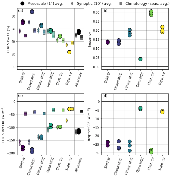
Figure 4Cloud radiative properties by cloud type: (a) CERES cloud fraction, (b) cloud frequency of occurrence, (c) average CERES net CRE per cloud type, (d) frequency-weighted net CRE. Each set of three symbols is for the 3 years (2014–2016) used. For panels (a) and (c), the mesoscale, synoptic, climatological averages are shown using circular, diamond, and square symbols, respectively (see Sect. 2e).
An issue with the compositing of observational data is that the cloud types do not all have the same geographic distribution. One approach would be to try to impose geographic parity by sampling the same number of points from some grid or else to control for every other variable by stratifying the data in many dimensions. The approach we adopted to identify the extent to which differences in potential driver variables reflect short-lived anomalies compared to geographic sampling bias was to calculate seasonal climatologies for each gridded dataset and then extract for each scene the climatological value of that field at that location. These were also composited by scene cloud type and compared to the composite of instantaneous values. This analysis is similar to the mesoscale vs. synoptic mean comparison described in the previous section but in this case using temporal deviations from local climatology. Figure 5a shows all three averages in the same panel for direct comparison. The black circles represent the mesoscale (i.e., average) sea surface temperature (SST) at that location and time, averaged over all classifications; the black diamonds are the same but averaged over a box, and the black squares correspond again to averages but with seasonal averages instead of daily values of SST.
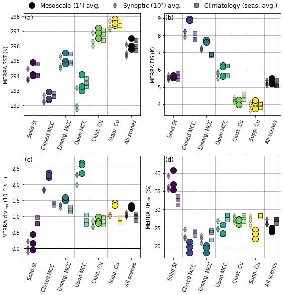
Figure 5Same as Fig. 4a but for (a) MERRA-2 sea surface temperature, (b) MERRA-2 estimated inversion strength (EIS), (c) MERRA-2 700 hPa divergence, and (d) MERRA-2 700 hPa relative humidity.
3.1 Climatology of occurrence
We first present the characteristics of the cloud types represented by the classifier categories. This complements the analysis of Yuan et al. (2020), which presents example scenes, cloud optical thickness, droplet effective radius, and absolute frequency for each cloud type. Figure 3 shows the relative frequency of occurrence of the six cloud types in the classification scheme. The most stratiform MCC types (Fig. 3a–d) occur at higher latitudes and towards the eastern SEP basin, while the two cumuliform types (Fig. 3e and f) dominate the warmer (sub) tropical oceans away from the continents, consistent with the ship-based climatology of Fig. 1. The location of the MCC types (with closed-cell upwind, open-cell downwind) is mostly consistent with their occurrence in the WH06 classifications. Both subtropical and midlatitude MCC are identified. The main differences with the WH06 classifications are that the disorganized MCC type, which previously included all scenes not classified as open MCC, closed MCC, or stratus, now primarily occurs near the Sc cloud deck instead of spreading over a much larger region. Another significant departure is that open-cellular MCC occurs much less frequently than in the WH06 classifier, representing only 4 % of all scenes. The solid stratus type is a mix of coastal stratus and midlatitude frontal stratus.
An ideal cloud type classification scheme would produce useful discrimination among cloud types in all regions as opposed to having different cloud types each dominating one region. One way to visualize how well this classification scheme embodies this property is by considering, for each region, the fraction of all scenes which come from the most common cloud type in that region and then from the top two most common, etc. This is shown in Fig. 6. Figure 6a shows the fraction of scenes covered by the dominant cloud type for that grid box. In Fig. 6b, we see that in the northwestern corner of our region of interest, the top two cloud types (in this case, suppressed and clustered Cu) account for more than 90 % of all scenes. This suggests that any further differentiation into more specific cloud subtypes would be most effective if focused on this region. Figure 6c and d show that the region with the greatest variability in cloud type is the zonal band near 45∘ S as well as the subtropical Sc–Cu transition region near 15∘ S.
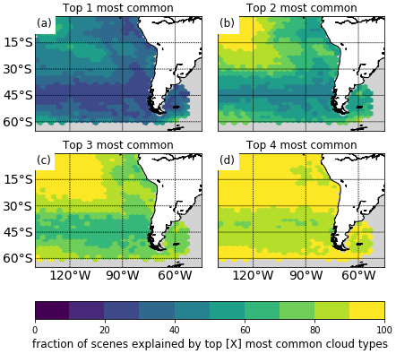
Figure 6The fraction of cloud scenes for each grid point, which are represented by (a) the most common cloud type for that grid point and (b–d) the top two through top four most common cloud types. Gray areas indicate that fewer than 200 scenes were sampled.
3.2 Sample case
To better illustrate the scale at which the classifications and the underlying data exist, Fig. 7 shows a case study from 22 July 2015. Each panel shows the classifications in colored circles, marking the center of each rectangular MODIS image on which the classifications are carried out (see Yuan et al., 2020, for additional details on classification).
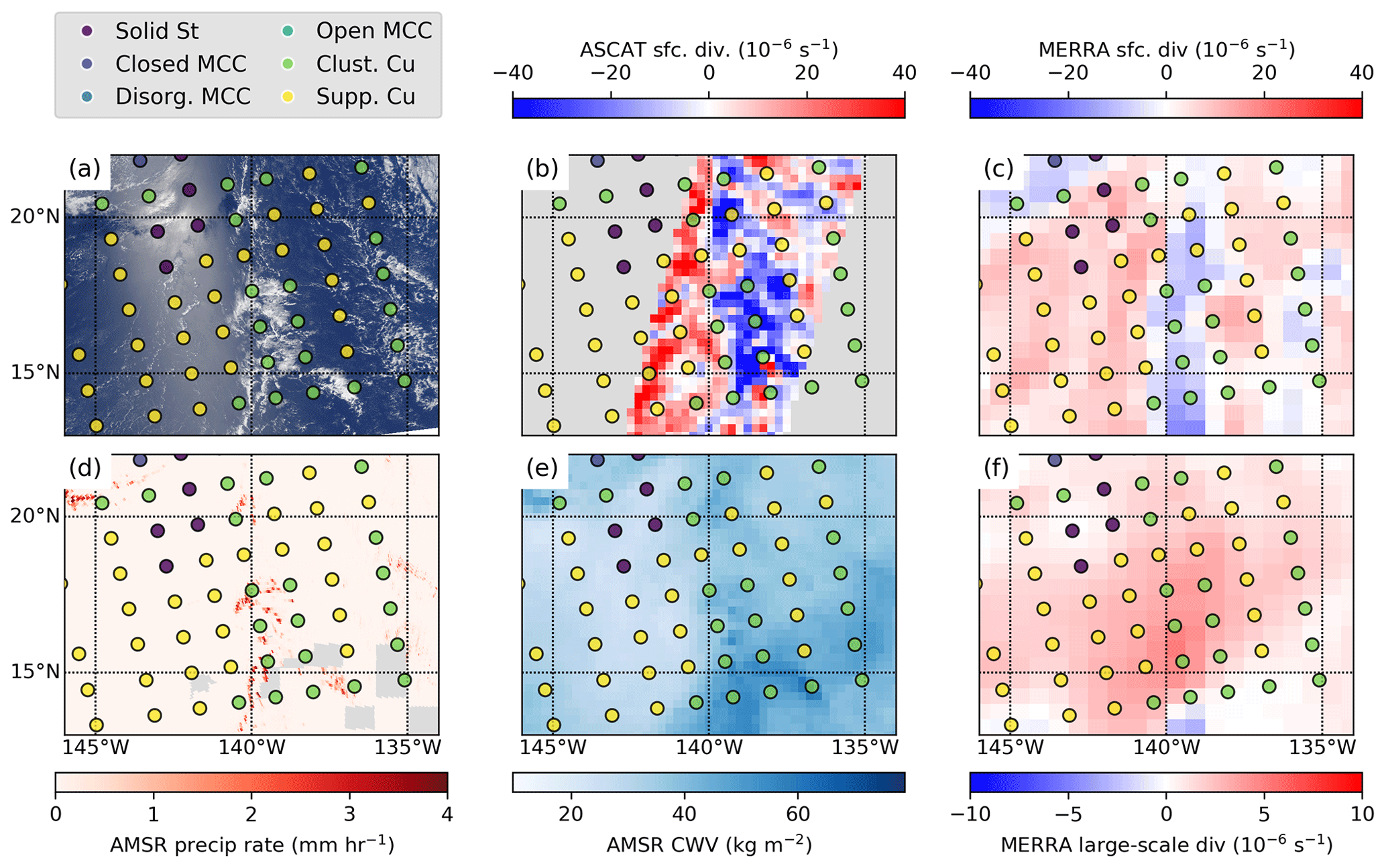
Figure 7Sample region observed on 22 July 2015 showing classifications (every panel, in colored circles). (a) MODIS true-color reflectance, (b) ASCAT surface divergence, (c) MERRA-2 surface divergence, (d) AMSR-2 89 Ghz precipitation rate, (e) AMSR-2 column water vapor, (f) MERRA-2 700 hPa divergence.
The scene selected highlights suppressed and clustered types. In Fig. 7a, a roughly 200 km by 400 km region of enhanced cloud in the lower middle of the scene is identified as clustered Cu, surrounded by suppressed-Cu scenes. A misidentification of sun glint as solid stratus is evident as well (though Fig. 3 shows that very few misidentifications of this type occur in tropical scenes to have a significant impact on the classification climatology). Figure 7b and c show the surface divergence as inferred from ASCAT and the MERRA-2 reanalysis; the ASCAT overpass time at 09:30 LT, being 4 h ahead of the MODIS-Aqua observation time, causes a slight geographic mismatch. Nevertheless, both surface divergence plots show strong convergence (in blue) in the clustered region and divergence in surrounding regions. Note also the noisy nature of the ASCAT observations as well as the narrow swath of ASCAT not allowing matches with many (approximately half) of the classifications. Figure 7f shows the large-scale divergence as inferred from the 700 hPa vertical motion. Although there is some convergence aloft at the southern boundary of the scene (where the MERRA-2 surface convergence is strongest), the remainder of the clustered region shows slightly enhanced subsidence aloft, in contrast to surface conditions, which as we see later is also the mean behavior for clustered scenes. MODIS indicates cloud top pressures between 800 and 700 hPa (not shown) at around 15∘ N, 138∘ W (where the divergence is strongest), consistent with the schematic model in BB17 (their Fig. 10). This divergence may potentially represent the outflow from the aggregated convection in this clustered region.
Figure 7d and e show the AMSR-2 precipitation and moisture retrievals, respectively. The clustered (suppressed) classifications are consistently associated with a moist (dry) CWV anomaly, and precipitation is only found in the clustered regions. Overall, the mesoscale anomalies are clearly resolved on the spatial scales of the classifications. Classification edge cases exist where a human observer would struggle to clearly identify a scene as suppressed or clustered; however on aggregate the machine learning classifications are consistent with human labeling, as the performance evaluation presented in Yuan et al. (2020) has shown.
3.3 Radiative properties of morphological cloud types
As the climatological relevance of marine low clouds relates in large part to their radiative effect, it is worth identifying the variability in radiative properties among the different categories. Figure 4 shows the low-cloud fraction of each cloud type, with closed MCC having the highest and suppressed Cu the lowest. The mean cloud fraction across all scenes (black dot at right of Fig. 4a) also shows that the Cu vs. Sc cloud types also split tidily into the below-average and above-average cloudy scenes for this particular sample, as expected. The mesoscale cloud fraction anomaly (represented by the difference between the small diamonds and circles for each type) shows that, on average, the scenes we classify are slightly cloudier than their surroundings. This is most pronounced for the closed MCC and most likely a result of the filtering of scenes with very low cloud. The only exception is suppressed Cu, which is associated with a low CF anomaly. The same is true when comparing to the climatological cloud fraction (small squares) where a high bias in cloud fraction is seen, again most likely due to the fact that we can only classify cloudy scenes.
Figure 4b–d show the composite net CRE of the various cloud types. In Fig. 4b the overall frequency of each cloud type in our dataset is broken down by year (2014–2016). Together, clustered- and suppressed-Cu scenes account for more than half of all scenes. Figure 4c shows the CERES net CRE as calculated in Sect. 2b for each type and year as well as the mesoscale and climatological value. The net CRE, mostly coming from the shortwave, broadly mirrors the cloud fraction. The total cooling averaged over all scenes is shown as the black dots in Fig. 4c, corresponding to a net CRE of W m−2. Note that due to the specific sampling strategy (only considering scenes with low cloud, without too much overlying high cloud) and the fact that we composite instantaneous daytime values that are not weighted by the global frequency of occurrence of our cloud types, our CRE for marine low clouds is approximately an order of magnitude larger than the global value found by L'Ecuyer et al. (2019).
The above difference between instantaneous local and global values underscores the fact that when considering the radiative importance of different cloud types, both frequency and mean CRE at the time of occurrence are relevant. Specifically, when considering the Cu cloud types (clustered and suppressed), which are the two types that are the most frequently occurring in our dataset, due to their dominance in the tropics and subtropics, one should keep in mind that their low mean instantaneous CRE is counterbalanced by their high frequency of occurrence. The frequency-weighted CRE (Fig. 4d), which is simply the product for each year of the data in Fig. 4b and c, is therefore appropriate as it represents the fraction of total cooling, over all scenes, by a particular cloud type. Thus open MCC, despite having a mean net CRE of −100 W m−2, only accounts for ∼5 W m−2 of the total cooling of all scenes in our dataset (approximately 4 %); while these scenes have high CFs and therefore net CRE, they are infrequent, more so in this classification compared to previous work. For the clustered and suppressed types, the importance of understanding their drivers is highlighted in Fig. 4d; clustered-Cu scenes have a contribution to the net CRE that is 5 times higher than suppressed-Cu scenes.
3.4 Composite analysis
Figures 5 and 8 are similar to Fig. 4, showing composites of meteorological variables by cloud type as well as synoptic and climatological averages (where seasonal mean values for a given location are composited instead of instantaneous values). For both these figures, we can estimate the variability between types explained by differences in geography by comparing the mesoscale averages (circles) to the climatological averages (squares). For instance, for every cloud type, there is almost no bias between the mesoscale and climatological averages of sea surface temperature (SST; Fig. 5a). In other words, variation in SST between scenes is almost entirely explainable by the variation in geography. The suppressed scenes occur over the warmest waters and the closed MCC over the coldest. The same is largely true for EIS, which is determined in part by SST. This is not surprising given the geographic distributions of the cloud types seen earlier and climatological gradients in SST and EIS. What this tells us, however, is that there is no strong evidence for subseasonal timescale perturbations to SST or EIS coinciding with variations in cloud type. We can also compare the mesoscale averages to the 10∘ synoptic averages to assess whether any mesoscale anomalies are coincident with cloud type variability. However, an important caveat to bear in mind is the bias introduced by our sampling strategy: only scenes with some low cloud and not too much high cloud are considered, whereas the surrounding scenes are not similarly constrained. These biases are best identified from the black “all scenes” markers. For instance, we notice in Fig. 5d that averaged over all scenes, RH700 is biased low by 3 %, most likely due to preferential selection of scenes with little high cloud (and therefore a free troposphere that is biased dry). This bias is also applicable to the climatological comparison. The dry free troposphere (FT) anomaly relative to the synoptic (and climatological) averages in, for example, the closed-MCC scenes can be explained by this sampling bias and is not indicative of some mechanism in a drier FT yielding closed-MCC clouds.
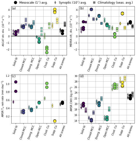
Figure 8Same as Fig. 5 but with (a) ASCAT surface wind divergence, (b) MERRA-2 surface wind divergence, (c) AMSR-2 rain rate, and (d) AMSR-2 column water vapor.
With that caveat in mind, Fig. 5 shows that closed MCC and to a lesser extent disorganized MCC are associated with a significant mesoscale anomaly in EIS (consistent with Muhlbauer et al., 2014). Solid stratus is associated with a positive anomaly in vertical motion and RH700 relative to climatology but not a mesoscale one, indicating that this link is driven by synoptic features; manual inspection confirms that many scenes identified as stratus are indeed associated with frontal systems. Both closed and open MCC are associated with strong subseasonal anomalies of enhanced subsidence, though again the absence of an anomaly relative to the synoptic mean indicates that these are larger features, likely associated with variability in the position of the subtropical high.
Aside from the mesoscale and subseasonal anomaly analysis, a key result is that clustered and suppressed types are poorly separated by the variables in Fig. 5; they have virtually identical EIS distributions, and though suppressed scenes are associated with slightly higher SST, large-scale divergence, and lower FT humidity, there is not much separation between them in this phase space, especially relative to the variability between all cloud types, and these small differences are consistent with their slightly different geographic distributions. In contrast, EIS is an excellent discriminator between the stratiform MCC types.
Composite analysis of the surface divergence, however, is much more helpful at distinguishing between the Cu cloud types. This is evident from Fig. 8a and b. From the ASCAT composite data, the strongest surface divergence is associated with suppressed scenes and the strongest convergence with the clustered scenes. When using MERRA-2 data, the only difference is that the closed-MCC cases have slightly stronger divergence, yet the clear separation between Cu types remains. Additionally, the surface divergence signal is clearly of a mesoscale nature and not explained by climatological differences, particularly for the convergence associated with clustered scenes; the synoptic environment shows broad divergence.
Having calculated both the 700 hPa large-scale and surface divergence, we can subtract the former from the latter to estimate a boundary layer anomaly divergence. If near-surface divergence purely reflects the large-scale subsiding flow, with no additional low-level circulation, we would expect this anomaly to be small. Figure 9a shows this surface level anomaly using both the MERRA-2 and ASCAT winds. The large positive anomaly for suppressed-Cu scenes indicates that the bulk of the divergence is a result of near-surface circulations rather than those extending over a deep layer of the lower troposphere; similarly for clustered Cu, the surface convergence together with mean large-scale divergence indicates a shallow circulation, as seen in the case study of Fig. 7.
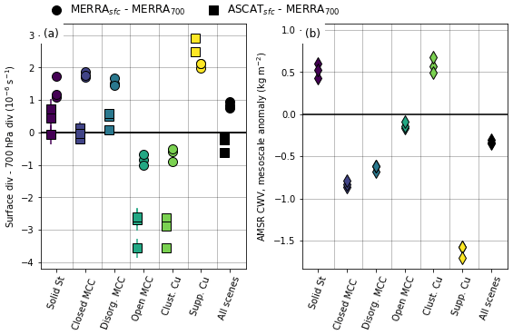
Figure 9(a) Surface divergence anomaly from 700 hPa (circles are based on MERRA-2 surface winds; squares are based on ASCAT surface winds). (b) AMSR-2 column water vapor mesoscale anomaly.
Considering AMSR-2 retrievals, the rain rate shows a very clear separation between clustered and suppressed cloud types, with a strong positive (negative) mesoscale anomaly for clustered (suppressed) Cu of around 0.4 mm d−1. Similar qualitative results are found for conditional rain rates and rain probabilities (not shown). It is worth noting that the resolution of the precipitation data is approximately 4 km, so the smallest clouds will not be resolved. The column water vapor results are interesting as well; consistent with the warm SSTs, both Cu cloud types occur in areas of high column water vapor. The mesoscale anomalies, however, are consistent with the BB17 presentation: clustered scenes are slightly moister than their environment and suppressed scenes slightly drier. This is difficult to identify in Fig. 8d, so Fig. 9b shows just the mesoscale anomaly for all cloud types and makes clear that the suppressed scenes are the most anomalously dry and the clustered scenes most anomalously moist. Although the moisture anomalies of the LES in BB17 were larger than those found here, this may be due to their mean state being moister. One finding from that work is that the amplitude of aggregation-associated moisture anomalies tended to scale with the mean state CWV, and so we expect that the higher mean state moisture in BB17 would occur with larger moisture anomalies.
3.5 Aircraft observations
Figure 10 shows the depth of the boundary layer and degree of decoupling (using the αq metric from Wood and Bretherton, 2004) based on CSET aircraft profiles. The parameter αq is a measure of relative resemblance of upper-boundary-layer moisture to the lower FT and lower boundary layer, with a value of 0 indicating a perfectly well-mixed boundary layer and a value of 1 indicating a perfectly decoupled boundary layer, where the upper-boundary-layer moisture is equal to the lower FT moisture.
For a given profile, the thermal inversion height is estimated using the maximum lapse rate, with the inversion being the layer where the lapse rate deviation from a moist adiabat exceeds 25 % of maximum deviation (this was tuned to agree with a visual assessment of the inversion layer and worked well for all profiles). Upper and lower BL in the qT equation are taken as the top and bottom 25 % of the BL depth, while the lower FT starts 500 m above the inversion top. While this method may not be the most precise in individual, more complex cumulus cases with more spatially and vertically heterogeneous moisture profiles, we use it for consistency and reproducibility. We also note that a joint histogram analysis of αq vs. cloud layer depth (not shown) produced consistent results to Wood and Bretherton (2004) and Park et al. (2004).
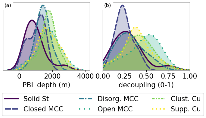
Figure 10Histograms of (a) boundary layer depth and (b) boundary layer decoupling index from CSET flights and dropsonde observations.
For each aircraft profile, the cloud type classification which covers that profile is selected for compositing, and so the profile represents a random estimate of depth or decoupling within that scene. Here the sample sizes are much smaller than the composites of satellite and reanalysis data, and so the full histograms are shown (smoothed using kernel density estimation) to highlight the uncertainty. Adopting a Lagrangian perspective, which accounts for the boundary layer evolving downstream of the trade winds through the Sc–Cu transition, boundary layer deepening and decoupling are found from stratus through closed, disorganized, and open MCC; in particular the degree of decoupling between closed and open MCC is very pronounced, with the former being the most coupled and the latter the most decoupled. However, this evolution breaks down for the Cu-type boundary layers, which are neither deeper nor more decoupled than open MCC. This is not surprising as the inversion at the top of the surface mixed layer where Cu clouds form will persist as the decoupled Sc layer is eroded, such that the remaining boundary layer stays shallower and strongly coupled to the surface. Also important to note is that, as with EIS and SST, clustered and suppressed types are difficult to distinguish by their depth and decoupling state, though clustered scenes are marginally deeper in Fig. 10a.
In this study we have analyzed the characteristics of the marine boundary layer for six different morphological cloud types, the occurrence of which was derived by novel machine learning-based cloud classification operating on MODIS mesoscale imagery. Specifically, we assessed whether the observations of clustered and suppressed cumulus are consistent with previous modeling of mesoscale aggregation of shallow cumulus. The key findings are as follows:
-
The six cloud types represent distinct MBL regimes, based on their geography and environmental conditions.
-
The anomalies in cloudiness, column water vapor, circulation, and precipitation are consistent with the Bretherton and Blossey (2017) LES results and conceptual model for mesoscale shallow aggregation.
-
Suppressed- and clustered-Cu scenes are most clearly separable by looking at surface wind divergence, and this signal is apparent in both satellite retrievals and the MERRA-2 reanalysis.
This last finding pertains to a more general conclusion, namely that, at least for the variables considered, mesoscale anomalies in meteorological variables are more pronounced for the cumulus types than the stratiform MCC types; this is true for CWV, precipitation, and surface divergence. For discriminating between the MCC types, EIS, depth, and decoupling are the most useful; in stratocumulus regions, these variables have been shown to correlate strongly with each other and with cloud cover (Wood and Bretherton, 2004; Wood and Hartmann, 2006).
Though it is tempting to conclude that surface divergence is such a good discriminator because the mesoscale aggregation described in BB17 is likely the most important determinant of cloud variability, we must also bear in mind that, along with precipitation, it is more an “internal” boundary layer predictor than most of the other predictors, e.g., EIS or SST, and therefore better coupled to other MBL state variables (e.g., cloud fraction). Additionally, it is also much more directly observed and resolved at a finer scale than, for example, 700 hPa vertical motion and therefore has a lower observational uncertainty. That being said, the strong consistency between the observations and the BB17 LES modeling of mesoscale shallow convection suggests that this process is an important driver of cumulus-dominated MBL cloud variability.
There are several limitations on the generalizability of these results. The first is that we have only considered the SEP and NEP regions, and other clouds, particularly those in the warmer trade wind regions of the western ocean basins, may have different MBL characteristics. The second is that we have only considered daytime behavior and cannot account for diurnal variability in cloud type. The observations from aircraft data were limited and did not extend south of Hawaii or north of California. Lastly, we have not examined in depth the role of SST in determining cloud type. This is not because it is unimportant (on the contrary, it is a key driver of most MCC variability; see McCoy et al., 2017) but rather because it does not vary much at mesoscale and short timescales.
With regards to climate modeling, CRE for different cloud types largely mirrors cloud fraction. While the CRE between suppressed and clustered types is very different, it remains to be seen whether the process of shallow convective aggregation affects synoptic-scale mean cloud cover and CRE. Given that models capable of reproducing such shallow aggregation are now able to run at global scales (Bretherton and Khairoutdinov, 2015), this question is best answered using simulation studies.
MODIS reflectance data for this work are available at https://doi.org/10.5067/MODIS/MYD021KM.006 (MCST/MODAPS, 2016). ASCAT data are available from http://www.remss.com/missions/ascat/ (last access: 2 December 2019) (Ricciardulli and Wentz, 2016). AMSR-2 water vapor data are available at http://www.remss.com/missions/amsr/ (Wentz et al., 2014). CERES SYN1deg data are available at https://doi.org/10.1175/JTECH-D-12-00136.1 (Doelling et al., 2013). MERRA-2 data are available at https://doi.org/10.5067/QBZ6MG944HW0 (GMAO, 2015). CSET aircraft data are available at https://doi.org/10.5065/D65Q4T96 (UCAR/NCAR EOL, 2017). Data processing code as well as processed classification data can be found on Zenodo at https://doi.org/10.5281/zenodo.4673556 (Mohrmann, 2021).
JM prepared the manuscript and performed most of the data analysis. RW provided continuous feedback and guidance during the analysis. TY and HS were responsible for the creation and processing of the classification dataset. RE provided the AMSR brightness temperature dataset and guidance on its proper use and interpretation. TY, HS, JM, RW, and LO all participated in the development of the classification methodology and subsequent interpretation and refinement of the classification dataset. All coauthors provided editorial feedback on the manuscript.
The authors declare that they have no conflict of interest.
We gratefully acknowledge our colleagues at the University of Washington for feedback and helpful discussion. Funding for this research was provided in part by the NASA MEaSUREs program. We acknowledge the use of imagery from the NASA Worldview application (https://worldview.earthdata.nasa.gov/, last access: 26 May 2020), part of the NASA Earth Observing System Data and Information System (EOSDIS). We are also very grateful to the anonymous reviewers for their valuable feedback, both scientific and editorial.
This research has been supported by the National Aeronautics and Space Administration (grant no. 80NSSC18M0084).
This paper was edited by Yafang Cheng and reviewed by two anonymous referees.
Agee, E. M.: Mesoscale cellular convection over the oceans, Dynam. Atmos. Ocean., 10, 317–341, https://doi.org/10.1016/0377-0265(87)90023-6, 1987.
Albrecht, B., Ghate, V., Mohrmann, J., Wood, R., Zuidema, P., Bretherton, C., Schwartz, C., Eloranta, E., Glienke, S., Donaher, S., Sarkar, M., McGibbon, J., Nugent, A. D., Shaw, R. A., Fugal, J., Minnis, P., Paliknoda, R., Lussier, L., Jensen, J., Vivekanandan, J., Ellis, S., Tsai, P., Rilling, R., Haggerty, J., Campos, T., Stell, M., Reeves, M., Beaton, S., Allison, J., Stossmeister, G., Hall, S., and Schmidt, S.: Cloud System Evolution in the Trades (CSET): Following the Evolution of Boundary Layer Cloud Systems with the NSF–NCAR GV, B. Am. Meteorol. Soc., 100, 93–121, https://doi.org/10.1175/BAMS-D-17-0180.1, 2019.
Bretherton, C. S. and Blossey, P. N.: Understanding Mesoscale Aggregation of Shallow Cumulus Convection Using Large-Eddy Simulation, J. Adv. Model. Earth Syst., 9, 2798–2821, https://doi.org/10.1002/2017MS000981, 2017.
Bretherton, C. S. and Khairoutdinov, M. F.: Convective self-aggregation feedbacks in near-global cloud-resolving simulations of an aquaplanet, J. Adv. Model. Earth Syst., 7, 1765–1787, https://doi.org/10.1002/2015MS000499, 2015.
Chen, T., Rossow, W. B., and Zhang, Y.: Radiative Effects of Cloud-Type Variations, J. Climate, 13, 264–286, https://doi.org/10.1175/1520-0442(2000)013<0264:REOCTV>2.0.CO;2, 2000.
Doelling, D. R., Loeb, N. G., Keyes, D. F., Nordeen, M. L., Morstad, D., Nguyen, C., Wielicki, B. A., Young, D. F., and Sun, M.: Geostationary Enhanced Temporal Interpolation for CERES Flux Products, J. Atmos. Ocean. Tech., 30, 1072–1090, https://doi.org/10.1175/JTECH-D-12-00136.1, 2013.
Eastman, R., Lebsock, M., and Wood, R.: Warm Rain Rates from AMSR-E 89-GHz Brightness Temperatures Trained Using CloudSat Rain-Rate Observations, J. Atmos. Ocean. Tech., 36, 1033–1051, https://doi.org/10.1175/JTECH-D-18-0185.1, 2019.
Emanuel, K., Wing, A. A., and Vincent, E. M.: Radiative-convective instability, J. Adv. Model. Earth Syst., 6, 75–90, https://doi.org/10.1002/2013MS000270, 2014.
Gelaro, R., McCarty, W., Suárez, M. J., Todling, R., Molod, A., Takacs, L., Randles, C. A., Darmenov, A., Bosilovich, M. G., Reichle, R., Wargan, K., Coy, L., Cullather, R., Draper, C., Akella, S., Buchard, V., Conaty, A., da Silva, A. M., Gu, W., Kim, G. K., Koster, R., Lucchesi, R., Merkova, D., Nielsen, J. E., Partyka, G., Pawson, S., Putman, W., Rienecker, M., Schubert, S. D., Sienkiewicz, M., and Zhao, B.: The modern-era retrospective analysis for research and applications, version 2 (MERRA-2), J. Climate, 30, 5419–5454, https://doi.org/10.1175/JCLI-D-16-0758.1, 2017.
GMAO – Global Modeling and Assimilation Office: MERRA-2 inst3_3d_asm_Np: 3d,3-Hourly,Instantaneous,Pressure-Level,Assimilation,Assimilated Meteorological Fields V5.12.4, GES DISC – Goddard Earth Sciences Data and Information Services Center, Greenbelt, MD, USA, https://doi.org/10.5067/QBZ6MG944HW0, 2015.
Hahn, C. J. and Warren, S. G.: A Gridded Climatology of Clouds over Land (1971–1996) and Ocean (1954–2008) from Surface Observations Worldwide (NDP-026E), OSTI dataset, USA, https://doi.org/10.3334/CDIAC/CLI.NDP026E, 2007.
Hahn, C. J., Rossow, W. B., and Warren, S. G.: ISCCP Cloud Properties Associated with Standard Cloud Types Identified in Individual Surface Observations, J. Climate, 14, 11–28, https://doi.org/10.1175/1520-0442(2001)014<0011:ICPAWS>2.0.CO;2, 2001.
Hartmann, D. L., Ockert-Bell, M. E., and Michelsen, M. L.: The Effect of Cloud Type on Earth's Energy Balance: Global Analysis, J. Climate, 5, 1281–1304, https://doi.org/10.1175/1520-0442(1992)005<1281:TEOCTO>2.0.CO;2, 1992.
L'Ecuyer, T. S., Hang, Y., Matus, A. V., and Wang, Z.: Reassessing the Effect of Cloud Type on Earth's Energy Balance in the Age of Active Spaceborne Observations. Part I: Top of Atmosphere and Surface, J. Climate, 32, 6197–6217, https://doi.org/10.1175/JCLI-D-18-0753.1, 2019.
LeMone, M. A. and Meitin, R. J.: Three Examples of Fair-Weather Mesoscale Boundary-Layer Convection in the Tropics, Mon. Weather Rev., 112, 1985–1998, https://doi.org/10.1175/1520-0493(1984)112<1985:TEOFWM>2.0.CO;2, 1984.
McCoy, I. L., Wood, R., and Fletcher, J. K.: Identifying Meteorological Controls on Open and Closed Mesoscale Cellular Convection Associated with Marine Cold Air Outbreaks, J. Geophys. Res.-Atmos., 122, 11678–11702, https://doi.org/10.1002/2017JD027031, 2017.
MCST/MODAPS – Characterization Support Team/MODIS Adaptive Processing System: MODIS/Aqua Calibrated Radiances 5-Min L1B Swath 1 km, Dataset, https://doi.org/10.5067/MODIS/MYD021KM.006, 2016.
Mohrmann, J: jkcm/mesoscale-morphology: (Version 1.0), Zenodo, https://doi.org/10.5281/zenodo.4673556, 2021.
Mohrmann, J., Bretherton, C. S., McCoy, I. L., McGibbon, J., Wood, R., Ghate, V., Albrecht, B., Sarkar, M., Zuidema, P., and Palikonda, R.: Lagrangian Evolution of the Northeast Pacific Marine Boundary Layer Structure and Cloud during CSET, Mon. Weather Rev., 147, 4681–4700, https://doi.org/10.1175/MWR-D-19-0053.1, 2019.
Muhlbauer, A., McCoy, I. L., and Wood, R.: Climatology of stratocumulus cloud morphologies: microphysical properties and radiative effects, Atmos. Chem. Phys., 14, 6695–6716, https://doi.org/10.5194/acp-14-6695-2014, 2014.
Nicholls, S. D. and Young, G. S.: Dendritic Patterns in Tropical Cumulus: An Observational Analysis, Mon. Weather Rev., 135, 1994–2005, https://doi.org/10.1175/MWR3379.1, 2007.
Park, S., Leovy, C. B., and Rozendaal, M. A.: A New Heuristic Lagrangian Marine Boundary Layer Cloud Model, J. Atmos. Sci., 61, 3002–3024, https://doi.org/10.1175/JAS-3344.1, 2004.
Platnick, S., Meyer, K. G., King, M. D., Wind, G., Amarasinghe, N., Marchant, B., Arnold, G. T., Zhang, Z., Hubanks, P. A., Holz, R. E., Yang, P., Ridgway, W. L., and Riedi, J.: The MODIS Cloud Optical and Microphysical Products: Collection 6 Updates and Examples From Terra and Aqua, IEEE T. Geosci. Remote, 55, 502–525, https://doi.org/10.1109/TGRS.2016.2610522, 2017.
Ricciardulli, L. and Wentz, F. J.: Remote Sensing Systems ASCAT C-2015 Daily Ocean Vector Winds on 0.25 deg grid, version 02.1, Remote Sens. Syst., St. Rosa, CA, available at: http://www.remss.com/missions/ascat/ (last access: 2 December 2019), 2016.
Stevens, B., Bony, S., Brogniez, H., Hentgen, L., Hohenegger, C., Kiemle, C., L'Ecuyer, T. S., Naumann, A. K., Schulz, H., Siebesma, P. A., Vial, J., Winker, D. M., and Zuidema, P.: Sugar, gravel, fish and flowers: Mesoscale cloud patterns in the trade winds, Q. J. Roy. Meteorol. Soc., 146, 141–152, https://doi.org/10.1002/qj.3662, 2020.
UCAR/NCAR EOL – Earth Observing Laboratory: Low Rate (LRT – 1 sps) Navigation, State Parameter, and Microphysics Flight-Level Data, Version 1.2, UCAR/NCAR – Earth Observing Laboratory, https://doi.org/10.5065/D65Q4T96, 2017.
Warren, S. G., Hahn, C. J., London, J., Chervin, R. M., and Jenne, R. L.: Global distribution of total cloud cover and cloud type amounts over the ocean, NCAR Technical Note, NCAR-TN 317, https://doi.org/10.2172/5415329, 1988.
Wentz, F. J., Meissner, T., Gentemann, C., Hilburn, K. A., and Scott, J.: Remote Sensing Systems GCOM-W1 AMSR2 Daily Environmental Suite on 0.25 deg grid, version 8, Remote Sens. Syst., St. Rosa, CA, available at: http://www.remss.com/missions/amsr/ (last access: 29 January 2020), 2014.
Wood, R. and Bretherton, C. S.: Boundary Layer Depth, Entrainment, and Decoupling in the Cloud-Capped Subtropical and Tropical Marine Boundary Layer, J. Climate, 17, 3576–3588, https://doi.org/10.1175/1520-0442(2004)017<3576:BLDEAD>2.0.CO;2, 2004.
Wood, R. and Bretherton, C. S.: On the Relationship between Stratiform Low Cloud Cover and Lower-Tropospheric Stability, J. Climate, 19, 6425–6432, https://doi.org/10.1175/JCLI3988.1, 2006.
Wood, R. and Hartmann, D. L.: Spatial variability of liquid water path in marine low cloud: The importance of mesoscale cellular convection, J. Climate, 19, 1748–1764, https://doi.org/10.1175/JCLI3702.1, 2006.
Wood, R., Köhler, M., Bennartz, R., and O'Dell, C.: The diurnal cycle of surface divergence over the global oceans, Q. J. Roy. Meteorol. Soc., 135, 1484–1493, https://doi.org/10.1002/qj.451, 2009.
Yuan, T., Song, H., Wood, R., Mohrmann, J., Meyer, K., Oreopoulos, L., and Platnick, S.: Applying deep learning to NASA MODIS data to create a community record of marine low-cloud mesoscale morphology, Atmos. Meas. Tech., 13, 6989–6997, https://doi.org/10.5194/amt-13-6989-2020, 2020.