the Creative Commons Attribution 4.0 License.
the Creative Commons Attribution 4.0 License.
 | 28 Jun 2021
Processes influencing lower stratospheric water vapour in monsoon anticyclones: insights from Lagrangian modelling
Aurélien Podglajen
Cristina Peña-Ortiz
Felix Ploeger
We investigate the influence of different chemical and physical processes on the water vapour distribution in the lower stratosphere (LS), in particular in the Asian and North American monsoon anticyclones (AMA and NAMA, respectively). Specifically, we use the chemistry transport model CLaMS to analyse the effects of large-scale temperatures, methane oxidation, ice microphysics, and small-scale atmospheric mixing processes in different model experiments. All these processes hydrate the LS and, particularly, the AMA. While ice microphysics has the largest global moistening impact, it is small-scale mixing which dominates the specific signature in the AMA in the model experiments. In particular, the small-scale mixing parameterization strongly contributes to the water vapour transport to this region and improves the simulation of the intra-seasonal variability, resulting in a better agreement with the Aura Microwave Limb Sounder (MLS) observations. Although none of our experiments reproduces the spatial pattern of the NAMA as seen in MLS observations, they all exhibit a realistic annual cycle and intra-seasonal variability, which are mainly controlled by large-scale temperatures. We further analyse the sensitivity of these results to the domain-filling trajectory set-up, here-called Lagrangian trajectory filling (LTF). Compared with MLS observations and with a multiyear reference simulation using the full-blown chemistry transport model version of CLaMS, we find that the LTF schemes result in a drier global LS and in a weaker water vapour signal over the monsoon regions, which is likely related to the specification of the lower boundary condition. Overall, our results emphasize the importance of subgrid-scale mixing and multiple transport pathways from the troposphere in representing water vapour in the AMA.
- Article
(16062 KB) - Full-text XML
- BibTeX
- EndNote


Water vapour in the upper troposphere–lower stratosphere (UTLS) is one of the most important chemical species because of its impact on the global radiative budget (Solomon et al., 2010; Riese et al., 2012). Its distribution depends on the strength of the Brewer–Dobson circulation, the quasi-horizontal isentropic transport between tropical and high latitudes and the convective activity that enhances the cross-isentropic transport (Fueglistaler and Haynes, 2005; Diallo et al., 2018; Poshyvailo et al., 2018). The Brewer–Dobson circulation lifts up moist air from the troposphere into the deep stratosphere through the Tropical Tropopause Layer (TTL). While crossing the TTL, air masses encounter the cold temperatures of the tropopause, the so-called Cold Point Tropopause (CPT) (Fueglistaler et al., 2005), resulting in ice formation, sedimentation and dehydration of the ascending air parcels. A number of studies have shown that, at first order, water vapour entering the stratosphere responds to the variability in CPT temperature (e.g. Mote et al., 1996; Fueglistaler and Haynes, 2005; Randel and Park, 2019). In particular, the pronounced annual cycle of tropical tropopause temperature is responsible for dry and wet anomalies which propagate upward in the tropical lower stratosphere, forming the water vapour tape recorder (Mote et al., 1996). However, the control of water vapour anomalies by the CPT weakens during boreal summer, when maxima of water vapour in the UTLS are found over the Asian and North American monsoon regions (Randel and Park, 2019). This raises the question of the importance of the monsoon systems as a secondary pathway to transport water vapour into the LS.
Monsoon circulations appear as a dynamical response to diabatic heating released by persistent convection over regions close to the Equator (Gill, 1980). In the case of the Asian Monsoon, convection has its climatological centre over the Bay of Bengal and generates the AMA, a strong planetary-scale anticyclone in the UTLS which is the most dominant feature in the global atmosphere during boreal summer (Hoskins and Rodwell, 1995). The rapid vertical transport in the inner core of the monsoon pumps up moist air masses from the troposphere directly into the UTLS. There, the strong anticyclonic winds of the monsoon circulation behave as a transport barrier (Ploeger et al., 2015) that isolates the air masses from outer regions, keeping the air with high water vapour content (and similar for other trace gases with tropospheric sources) confined (Randel and Park, 2006; Park et al., 2007; Randel et al., 2010; Santee et al., 2017). At this height, air masses slowly ascend through the cold tropopause, where they further dehydrate (Park et al., 2007). However, the mechanism of simple large-scale temperature control alone might not be sufficient to explain water vapour distributions by themselves as air masses in the Asian Monsoon UTLS are generally about 20 %–50 % supersaturated (e.g. Krämer et al., 2020). In the case of the North American Monsoon Anticyclone (NAMA), there is less understanding of the water vapour signal observed, which is much stronger than for air under purely saturated conditions (Gettelman et al., 2004). However, as the anticyclonic circulation in the UTLS of the North American Monsoon is much weaker, the sensitivity to processes also present in the Asian Monsoon, such as convection, is different (Dessler and Sherwood, 2004; Randel et al., 2012). Thus, besides tropical cold-point temperatures, multiple other factors influence the transport of water vapour to the LS.
The impact of convection has been the focus of several studies but remains controversial. While Dessler and Sherwood (2004), Dessler et al. (2007), Ueyama et al. (2018) and Gettelman et al. (2002a) found that convection, and especially overshooting events, increase the LS water vapour signal over the monsoon regions, other studies emphasized that the main role of convection is related to changes in diabatic heating rates and, hence, the dynamical structure of the region (Gettelman et al., 2002b; Park et al., 2007; Schoeberl et al., 2013; Randel et al., 2015; Zhang et al., 2016; Kim et al., 2018). Randel et al. (2015) found that stronger convection leads to relatively cold temperatures in the subtropical LS, which they identified as a key region controlling large-scale dehydration within the anticyclonic monsoonal circulation, giving rise to a drier stratosphere. Therefore, it is not clear whether the main role of convection is to moisten the LS through overshooting events or to dehydrate it by decreasing the tropopause temperatures.
Furthermore, Ueyama et al. (2018) concluded from Lagrangian experiments that convective hydration is necessary to explain the water vapour signal over monsoon regions. On the other hand, James et al. (2008) found that process to be of second order, and other studies achieved realistic H2O distributions without any convective scheme (Schoeberl et al., 2013; Ploeger et al., 2013; Poshyvailo et al., 2018). Thus, this apparent disagreement not only highlights the problem of understanding the role of convection in LS water vapour simulations, but also the impact that the configuration of a model experiment might have on the LS water vapour distribution. Schoeberl et al. (2013) use the model developed by Schoeberl and Dessler (2011) based on the domain-filling Lagrangian technique. This approach is based on the philosophy that LS water vapour depends on the processes acting in the upper troposphere and in the tropopause region and therefore assumes only a minor role of the lower- to mid-tropospheric water vapour distribution and the specific model set-up of air parcel release at locations close to but below the tropopause. This approach has been successfully applied to answer many questions related to the water vapour distribution in the TTL (Schoeberl and Dessler, 2011; Schoeberl et al., 2012, 2013, 2014, 2018, 2019; Zhang et al., 2016; Wang et al., 2019), but it has never been compared in detail to consistent models covering the whole troposphere as well.
Another relevant process to the water vapour budget is ice microphysics (in particular, sedimentation and detrainment) in the UTLS related to the formation of cirrus clouds. Ice could be convectively lofted (Corti et al., 2008; Dessler et al., 2007, 2016; Ueyama et al., 2018; Wang and Dessler, 2012; Schoeberl et al., 2019) or in situ formed (Wang and Dessler, 2012; Ploeger et al., 2013; Krämer et al., 2020). In the first case, it is not clear whether evaporation of ice injected into the LS by overshoots leads to a moistening of the LS (Corti et al., 2008; Wang and Dessler, 2012) or not (Ueyama et al., 2018). In the second case, cirrus clouds form in cold regions of the UTLS (Gettelman et al., 2002a), decreasing the water vapour present. However, depending on their properties, such as their thickness, cirrus clouds could lead to a warming of these regions (Krämer et al., 2020). This agrees with Ploeger et al. (2013), which showed from model simulations that evaporation of ice in the UTLS increases the water vapour everywhere, including the Asian Monsoon region. However, the relative role of this process, in contrast with other mechanisms, not only in net water vapour in monsoon anticyclones but also in its variability, has not been fully assessed yet.
Turbulence and the associated small-scale mixing result in diffusivity in the UTLS, which affects the transport of trace gas constituents, including water vapour, into the LS (Podglajen et al., 2017). Konopka et al. (2007) showed that a parameterization of the small-scale mixing between nearby air masses based on the strain- and shear-induced deformation of the large-scale flow led to an enhancement of cross-tropopause transport in the monsoon regions and in particular in the Asian Monsoon. This mechanism has been invoked to explain observed tracer distributions in the UTLS (Pan et al., 2006). As flow deformation is commonly found in the vicinity of the subtropical jet stream, which is very close to the tropopause, air masses tend to mix in these regions. As a consequence, air masses reach the LS with higher water vapour content, avoiding in some cases the coldest temperatures of the tropopause (Poshyvailo et al., 2018). However, as reported by Poshyvailo et al. (2018) and Riese et al. (2012), the final impact of mixing on water vapour largely depends on the mixing strength predefined in their simulations and is thus highly uncertain.
At mid-stratospheric levels, methane oxidation acts as a source of water vapour. Through the downwelling branch of the Brewer–Dobson circulation, these moistened air masses are transported into the LS and partly are further recirculated into the tropics (Ploeger et al., 2013). Despite the fact that this horizontal transport is not as strong as in the opposite direction, it has a non-negligible impact on the monsoon regions.
In this study, we use the Chemical Lagrangian Model of the Stratosphere (CLaMS) (McKenna et al., 2002b, a; Konopka et al., 2004) with the aim of describing and quantifying the contributions of the different physical processes to the water vapour distribution in the lower stratosphere and particularly over the Asian and American monsoons. For this purpose, we have performed five experiments to analyse the role of each of the following processes: large-scale temperatures, methane chemistry, ice microphysics (including effects of ice sedimentation and nucleation barrier), small-scale mixing processes, and in particular vertical tropospheric mixing (likely related to convection). Furthermore, we also assess the sensitivity of the LS water vapour signal to the domain-filling technique developed by Schoeberl and Dessler (2011). This approach has been widely used in the recent past (i.e. Zhang et al., 2016; Schoeberl et al., 2018; Wang et al., 2019), but the effects of this set-up on simulated water vapour distributions have not been studied in detail yet. To shed more light on the related effects, we developed a model version of CLaMS analogous to this forward-trajectory domain-filling approach, configured all the sensitivity experiments based on this model set-up and compared them with a multi-decadal full-blown chemistry transport model CLaMS simulation as used in Konopka et al. (2004), Diallo et al. (2018) and Tao et al. (2019). Besides, we used satellite observations from Aura Microwave Limb Sounder (MLS) to assess the reliability of each simulation.
The remainder of the paper is organized as follows. In Sect. 2, we present the domain-filling technique, the data and the configuration of the different experiments. In Sect. 3, we evaluate the different experiments in simulating LS water vapour and how they capture the variability of the water vapour signal over the Asian and North American monsoon regions. Finally, in Sect. 4, we discuss the relevance of the processes to simulate the water vapour signal and also the differences in water vapour found using the domain-filling technique and the standard version of CLaMS. It should be noted that we do not aim to provide a most realistic model here but rather carry out simplified sensitivity experiments to present estimates of the effects of various processes to be potentially included in models simulating water vapour in the monsoon UTLS.
2.1 The CLaMS model
To evaluate the sensitivity of lower stratospheric water vapour over monsoon regions to different physical processes, we use the Chemical Lagrangian transport model CLaMS (McKenna et al., 2002b; Konopka et al., 2004). This model simulates the three-dimensional trajectories of an ensemble of air parcels forward in time as well as the changes in the chemical composition of the air parcels along them. CLaMS has a modular structure that allows different parameterizations or new configurations to be easily implemented. Thus, the sensitivity of the water vapour distribution to each parameterization can be studied easily by switching them on and off.
The CLaMS model has been widely used to study the distribution of several tracers in the stratosphere (Riese et al., 2012), including recent studies on water vapour in the lower stratosphere (Tao et al., 2019; Poshyvailo et al., 2018). Previous studies have shown that the model properly simulates the variability of the stratospheric water vapour (Diallo et al., 2018; Tao et al., 2019) and the water vapour distribution over monsoon regions during boreal summer (Poshyvailo et al., 2018), highlighting the efficiency of these regions in transporting air masses and water vapour into the TTL (Ploeger et al., 2017; Nützel et al., 2019; Yan et al., 2019).
All experiments performed for the present study use 6-hourly winds and temperature from the European Centre for Medium-Range Weather Forecasts (ECMWF) ERA-Interim reanalysis (Dee et al., 2011). The model uses a vertical hybrid coordinate that follows the orography with a σ coordinate at the ground that transforms into potential temperature in the upper troposphere. Above σ=0.3 (about 300 hPa in regions without strong orography), the vertical coordinate is purely isentropic. Cross-isentropic transport is simulated using total diabatic heating rates (considering all-sky radiation, latent heat release, and diffusive and turbulent heat transport as detailed by Fueglistaler et al., 2009) from ERA-Interim forecast data, as described in Ploeger et al. (2010). For the sake of the analysis, simulated water vapour content of air parcels is daily gridded into maps with bin size 5∘ longitude × 2∘ latitude at a given pressure or potential temperature level with a thickness of 10 hPa or K, respectively. Hence, daily distributions of water vapour at 100 hPa are the result of averaging air parcels found between 105 and 95 hPa.
2.2 Domain-filling set-up
To create a common framework between previous studies focusing on the simulation of stratospheric water vapour (Schoeberl et al., 2013; Zhang et al., 2016; Wang et al., 2019) and our CLaMS sensitivity experiments, we have implemented the forward domain-filling technique, here referred to as Lagrangian trajectory filling (LTF), in CLaMS. This set-up, introduced by Schoeberl and Dessler (2011), has been widely used to study different properties of water vapour in the stratosphere and UTLS region (Schoeberl et al., 2012, 2013, 2014, 2018, 2019; Dessler et al., 2014; Zhang et al., 2016; Ye et al., 2018). In this approach, air parcels are continuously launched at a given level below the tropopause, and their trajectories are calculated forward in time until they leave the domain of interest, here bounded by the surfaces p=250 hPa (lower boundary) and θ=1800 K. After a spin-up time during which the number of tracked air parcels increases, an equilibrium state is reached in which the release of new air parcels balances removal at the boundaries. At that point, due to the structure of the large-scale stratospheric circulation, the whole domain is filled with air parcels.
McKenna et al., 2002aTable 1Description of experiments done with CLaMS.
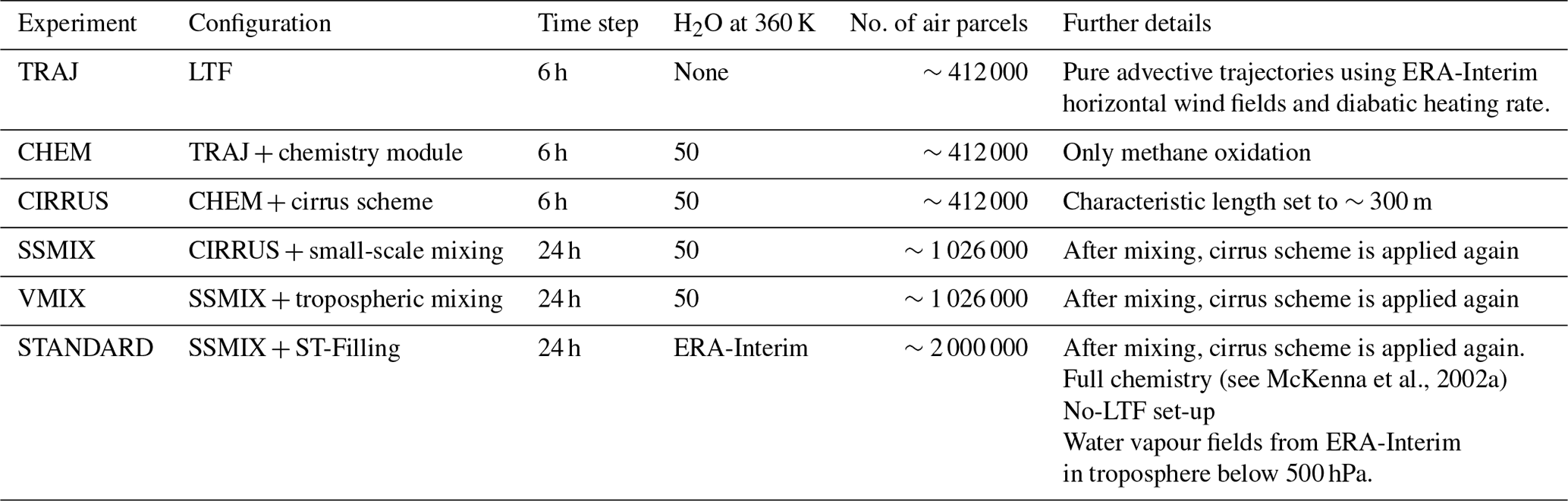
Time step specifies the frequency of the output in each experiment. No. of air parcels is the mean number of air parcels per day after 2 years of spin-up time. LTF (Lagrangian
trajectory filling set-up): based in the domain-filling technique developed by Schoeberl and Dessler (2011). ERA-Interim reanalysis from the European Centre for Medium-Range
Weather Forecasts.
Our set-up closely follows that of Schoeberl and Dessler (2011). Once a day (at 12:00 UTC), air parcels are released on a regular 5∘ longitude × 2∘ latitude grid spanning the 60∘ S–60∘ N latitudinal band. We initialize on the θ=360 K surface, which is, on average, above the level of zero radiative heating (LZRH) (Gettelman et al., 2002a) but below the tropical tropopause (∼375–380 K). We simulate the period from 2005 to 2016. The spin-up time is about 2 years, similar to Schoeberl and Dessler (2011). In pure LTF simulations, the equilibrium number of tracked air parcels is about 400 000 (500 000 in Schoeberl and Dessler, 2011), but in the case of experiments including small-scale mixing parameterizations, that number increases to 1.6 million (Table 1) due to the spawning of new parcels inside the domain, which adds up to the release at θ=360 K.
2.3 Experiments
We performed five LTF experiments with CLaMS. A summary of all experiments is provided in Table 1. This set of experiments is configured in such a way that the tested parameterizations are added cumulatively, increasing the complexity of the simulations and number of included processes step by step.
2.3.1 Pure trajectory (LTF) experiments: TRAJ, CHEM and CIRRUS
The first set of three experiments (called TRAJ, CHEM and CIRRUS) uses a pure LTF with advective trajectories launched exclusively at θ=360 K. While they are based on the same trajectories and hence transport, they differ in their treatment of chemical and microphysical processes impacting water vapour.
In TRAJ, chemistry and detailed microphysics are essentially ignored. Air parcels are initialized with 50 ppmv water vapour at the launch level. Thereafter, water vapour in excess of saturation (100 % relative humidity, RH) is removed at each time step. From a microphysical point of view, this is equivalent to assuming instantaneous formation and fall-out of all ice particles at 100 % RH. Note that this approach is, in practice, equivalent to setting to the lowest saturation mixing ratio (LMR) encountered by the air parcel along its trajectory, as in Fueglistaler and Haynes (2005). Saturation mixing ratios over ice are estimated from the 6-hourly ERA-Interim temperature and pressure following Murphy and Koop (2005).
In CHEM, the moistening effect of methane oxidation is included by applying the CLaMS chemistry module (Pommrich et al., 2014). The corresponding reactions are a significant source of water vapour in the middle and upper stratosphere. The methane mixing ratio at launch level is taken to be 1.7 ppmv, following Schoeberl et al. (2013). As in TRAJ, water vapour in excess of 100 % relative humidity is removed at each time step. The CLaMS dehydration scheme (for details, see Von Hobe et al., 2011) is configured equivalently to the LMR calculation in the basic TRAJ case. Therefore, an air parcel is set to saturation whenever its water vapour content is above 100 % of RH, following Marti and Mauersberger (1993), which is similar to Murphy and Koop (2005).
The third experiment, CIRRUS, applies the same initialization and simplified chemistry as CHEM. However, it also takes into account the ice phase (although simplified): in case of supersaturation, excess water vapour is instantaneously transferred to the ice phase, instead of being removed, as described in Von Hobe et al. (2011). Then, a mean (spherical) ice particle size and the corresponding settling velocity are computed using an empirically defined ice particle density (not temperature-dependent) based on in situ observations (Krämer et al., 2009). The calculated sedimentation length of the ice particles during one time step is compared to a characteristic length (∼300 m, optimized by Ploeger et al., 2013) to yield the fraction of ice removed from the air parcel (e.g. if the sedimentation length is one-third of the characteristic length, 30 % of the ice is assumed to fall out). If during the following time steps an air parcel turns out to be subsaturated and ice exists, all ice evaporates till the air parcel reaches saturation.
It should be noted that this simplified microphysics scheme does not resolve the nucleation and growth of the ice particles, only their sedimentation. Consistently, it also does not include the effect of temperature fluctuations due to gravity waves (Jensen and Pfister, 2004) unresolved in the reanalysis. Although those are ubiquitous (e.g. Podglajen et al., 2016; Schoeberl et al., 2017), it is not straightforward to include them in the simplified microphysics scheme, in particular due to their complicated interaction with ice nucleation and ice crystal number density (Dinh et al., 2016; Jensen et al., 2016). Furthermore, earlier studies have argued that their impact on water vapour itself is marginal (Fueglistaler and Baker, 2006) and that they mainly affect the ice cloud cover (e.g. Schoeberl et al., 2016, 2018). We therefore refrain from including gravity-wave-induced temperature fluctuations but regard them as an additional uncertainty for our study.
2.3.2 Experiments including small-scale mixing effects: SSMIX, VMIX and STANDARD
One of the key features of the CLaMS model is its parameterization of small-scale mixing processes (McKenna et al., 2002b; Konopka et al., 2004, 2007). This parameterization has been proposed to include the effects of small-scale mixing on tracer distributions, mainly in regions where large-scale flow deformations occur (Konopka et al., 2004, 2007; Pan et al., 2006).
Details about the mixing parameterization and its consequence in terms of diffusivity can be found in McKenna et al. (2002b), Konopka et al. (2004), Konopka et al. (2007) and Poshyvailo et al. (2018), and we only briefly summarize the governing principle here. The relative position of each parcel and its nearest neighbour are tracked during advection by the reanalysis wind over a 24 h time step. Due to vertical wind shear and horizontal deformation, the horizontal distance between the air parcel and its nearest neighbours after advection changes. If this distance falls below a threshold distance , both air parcels are merged into one parcel at the midpoint. If the distance exceeds , a new air parcel is inserted in the middle. This adaptive regridding is the core piece of the mixing scheme and ensures that the horizontal distance between parcels remains of the order of r0 while allowing for some deformation. The composition of the new air parcel, i.e. its mixing ratios of water vapour, methane and ice, is set to the average of the mixing ratios of the parcels that experienced mixing.
The fourth experiment, SSMIX, adds the small-scale mixing parameterization of CLaMS to the processes represented in CIRRUS. After a mixing event, the same dehydration scheme as in CIRRUS is applied again to remove the supersaturation that may have been introduced in new air parcels due to the mixing and bypassing cold temperatures. Transient temperature fluctuations in turbulent layers are neglected but are likely short-lived and not causing a significant effect.
The fifth experiment, called VMIX, includes enhanced tropospheric mixing recently developed by Konopka et al. (2019). This additional parameterization relates tropospheric mixing to unresolved convective instability. In this VMIX experiment, air parcels with a (moist) Brunt–Väisälä frequency, , larger than a predefined value, , undergo tropospheric mixing with their nearest neighbours: their chemical composition is changed to the averaged mixing ratios of all the parcels involved in the mixing process. Contrary to the standard mixing scheme, this procedure does not change the position of the air parcels.
Finally, besides the above experiments based on the LTF set-up, we consider the full-blown chemistry transport model standard version of CLaMS (STANDARD) (Diallo et al., 2018; Tao et al., 2019). This simulation includes the same parameterizations as SSMIX but has a different initialization. The air parcels are released at the beginning of the simulation throughout the domain, covering both the troposphere and stratosphere, with a horizontal resolution of about 100 km in the UTLS (for details, see e.g. Konopka et al., 2019). Once released, trajectories of air parcels are computed using reanalysis horizontal wind fields and diabatic heating rates for vertical transport. When air parcels are in the troposphere below about 500 hPa, their water vapour content is interpolated from ERA-Interim, while methane is derived from ground-level observations. The CLaMS dehydration and chemistry schemes are applied, configured consistently with the CIRRUS experiment. Note that, contrary to the LTF technique, the boundary of the model is the surface such that air parcels are not filtered out when they reach below 250 hPa or above 1800 K (as in the LTF experiments), and the water vapour content of air parcels at 360 K is not fixed uniformly to 50 ppmv but calculated consistently in the model. Here we will refer to this set-up as “Stratosphere–Troposphere Filling” (ST-Filling). Further details of the initialization can be found in Pommrich et al. (2014).
2.4 Aura MLS observations
Satellite observations of water vapour mixing ratios in the LS from Aura Microwave Limb Sounder (Waters et al., 2006) are used to further assess the results. We use version 4.2 of the water vapour data from MLS (Lambert et al., 2015), which has been fully described in Livesey et al. (2018). These water vapour products have been validated in several studies and recently have been part of a climatological overview of the Asian Monsoon Anticyclone (Santee et al., 2017). Here, Aura MLS data and CLaMS data have been compiled on the same regular latitude–longitude grid as the one used by the experiments. In particular, we use the MLS data on 100 and 82 hPa pressure levels and compare them to the simulated water vapour distributions at 100 and 80 hPa, respectively. Since we are interested in differences between set-ups, we did not apply the averaging kernels to the model outputs to avoid potential smearing out of fine-scale patterns. We note that applying the averaging kernels of MLS does not change the pattern of water vapour in the lower stratosphere during boreal summer.
3.1 Boreal summer climatology of lower stratospheric water vapour
Figure 1a–g show the climatological water vapour distribution at 100 hPa during June–August (JJA) over the 2007–2016 period in the different CLaMS experiments and MLS observations (i.e. excluding the spin-up). A similar figure for 80 hPa is presented in Fig. 2. All experiments (Fig. 1b–f) reproduce the main characteristics of the water vapour distribution found in MLS. The contrast between the dry tropics and subtropics and the moister mid and high latitudes seen in MLS is present in all simulations. Furthermore, all experiments, including TRAJ, exhibit a local maximum in the Asian Monsoon Anticyclone (AMA). This consistency between the different experiments emphasizes the key role of transport through the large-scale temperature field in causing this feature (as found in e.g. James et al., 2008). However, there are also important differences between the experiments and with MLS observations. Compared with MLS (Fig. 1a), experiments with the LTF scheme (Fig. 1b–f) underestimate the water vapour content in the moistest regions. This underestimation reaches 1.5 to 2 ppmv in the case of TRAJ, pointing either to biases in large-scale transport and temperatures in ERA-Interim or to missing processes, as expected. The dry bias is reduced in the more sophisticated experiments which include more processes. In addition, there is a misrepresentation of the NAMA in all experiments, which tend to show a weaker maximum shifted towards the eastern and central Pacific with respect to observations. It should be noted that at 80 hPa the agreement between STANDARD and MLS is much better (Fig. 2). Larger differences at 100 hPa are likely related to the fact that this lower pressure level is partly in the stratosphere and partly in the troposphere (e.g. in the Asian Monsoon where the tropopause is frequently above 100 hPa). Small biases in reanalysis tropopause height can therefore cause large biases in simulated water vapour at 100 hPa, while at 80 hPa their effect is marginal. Nevertheless, we focus our results at 100 hPa here as this is the most frequently considered level for investigating the monsoon UTLS, and further our goal is not to identify a best-case simulation scenario but to estimate the effects of different processes from the sensitivity simulations, and these estimates are very similar at 100 and 80 hPa.
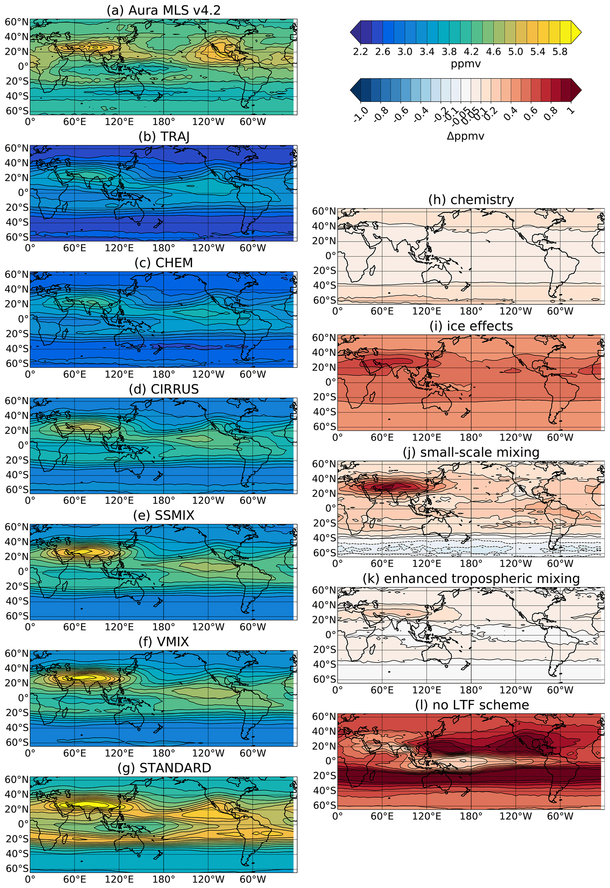
Figure 1(a–g) Climatology of water vapour distribution at 100 hPa during boreal summer (June–July–August) for the period 2007–2016 from (a) Aura MLS v4.2 observations, (b) TRAJ, (c) CHEM, (d) CIRRUS, (e) VMIX, (f) SSMIX and (g) STANDARD simulations. (h–l) Isolated effect of (h) methane oxidation, (i) cirrus, (j) small-scale mixing, (k) enhanced tropospheric mixing and (l) no-LTF scheme. Air parcels have been binned to a 5∘ longitude × 2∘ latitude grid.
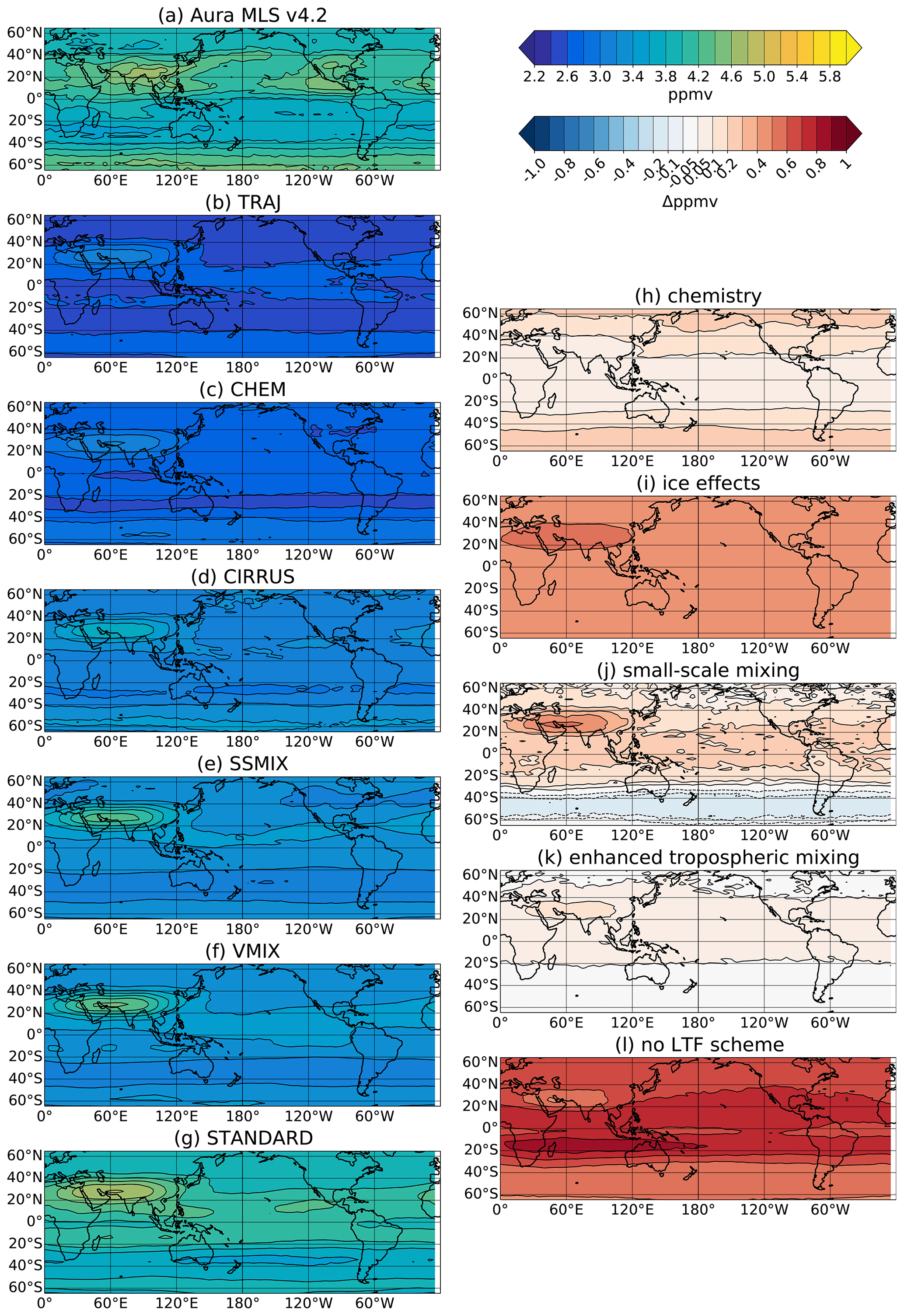
Figure 2(a–g) Climatology of water vapour distribution at 80 hPa during boreal summer (JJA) for the period 2007–2016 from (a) Aura MLS v4.2 observations, (b) TRAJ, (c) CHEM, (d) CIRRUS, (e) VMIX, (f) SSMIX experiments and (g) STANDARD simulation. (h–l) Isolated effect of each (h) chemistry, (i) cirrus, (j) small-scale mixing, (k) enhanced tropospheric mixing and (l) no-LTF scheme. Air parcels have been binned to a 5∘ longitude × 2∘ latitude grid.
In order to separate the effect of each parameterization, Fig. 1h–l display the differences between pairs of experiments which share the same configuration except for one single process parameterization. Thus, Fig. 1h (CHEM minus TRAJ) isolates the impact of methane oxidation, which is only included in CHEM (see Table 1). Similarly, Fig. 1i–k show the impact of the simplified ice microphysics (cirrus) parameterization (CIRRUS-CHEM), small-scale mixing (SSMIX-CIRRUS) and enhanced tropospheric mixing (VMIX-SSMIX), respectively.
Regarding methane oxidation, Fig. 1h shows a water vapour increase of around +0.1 ppmv over the tropics and subtropics that reaches +0.2 ppmv over high latitudes, as expected. As methane oxidation occurs at mid-stratospheric levels (Randel et al., 1998), its impact on the water vapour distribution at 100 hPa (Fig. 1h) is a consequence of air parcels moving downward from those altitudes following the downwelling branch of the Brewer–Dobson circulation at high latitudes. During boreal summer, the downward circulation is stronger in the Southern Hemisphere, which explains the larger increase in water vapour in this region. Once air parcels reach the lower stratosphere at high latitudes, some of them may reach the troposphere below 250 hPa, where they are removed from the simulation, while others follow the residual meridional circulation giving rise to the observed subtropical and tropical enhancements of water vapour at 100 hPa. This weak meridional transport was also observed by Ploeger et al. (2013) and Poshyvailo et al. (2018). A similar impact of methane oxidation can be found at 80 hPa in spite of the stronger meridional gradient at this pressure level (Fig. 2).
Including our simplified representation of ice microphysics (Fig. 1i) results in a further moistening of the LS ranging from +0.4 to +0.6 ppmv over most regions. These values are in agreement with the global increase of +0.5 ppmv found by Ploeger et al. (2013) and exceed the effect related to methane. Moreover, Fig. 1i shows that the effects of ice are especially large in the AMA (about +0.8 ppmv at 100 hPa), enhancing the moisture anomaly in the monsoon UTLS. This signature is also found at 80 hPa but with slightly weaker values compared to 100 hPa (Fig. 2i).
Small-scale mixing has a similar impact (Fig. 1j), increasing water vapour at latitudes north of 30∘ S and especially in the AMA. Outside of the AMA, the water vapour increase linked to small-scale mixing is slightly weaker than that attributed to ice microphysics (+0.1 to +0.4 ppmv). The local impact on water vapour in the AMA region, however, is stronger and reaches values above +0.9 ppmv at 100 hPa. This strong moistening effect can be attributed to the fact that mixing processes are more frequent in regions with large-scale flow deformations, which are mainly located in the surroundings of the subtropical jet (Konopka and Pan, 2012; Poshyvailo et al., 2018) and hence in the AMA.
The effects of the enhanced mixing in the troposphere as represented in the VMIX experiment are shown in Fig. 1k. An increase in water vapour of up to +0.1 ppmv occurs almost everywhere north of 30∘ S, with again a relatively stronger impact in the AMA, with differences larger than +0.3 ppmv. This stronger influence in the AMA compared to other regions is also found at 80 hPa but is weaker than at 100 hPa. Compared to other processes, VMIX shows a weak increase in water vapour in the AMA related to the enhanced tropospheric mixing. The reason behind this increase in lower stratospheric humidity with the mixing parameterizations in SSMIX and VMIX ultimately lies in the bypassing of cold traps which air parcels would have otherwise encountered along their slow ascent and the associated horizontal wandering (for further details, see Appendix A).
The 80 hPa level shows a similar spatial distribution of water vapour differences to that at 100 hPa, with values peaking again in the AMA (Fig. 2j). However, the relative strength of this maximum (+0.5 ppmv) is weaker than at 100 hPa.
Since mixing changes the temperature encountered by air parcels, the impact of temperature-dependent processes, such as ice microphysics, is altered. To evaluate this effect, we have run a 2-year simulation, hereafter called “VMIXnocirrus”, in which all the water vapour in excess of saturation is instantaneously removed instead of being transferred to the ice phase. The difference between VMIXnocirrus and VMIX shows the impact of ice transport, as CIRRUS-CHEM, but with mixing being applied (see Fig. A2). Comparing Fig. A2 with Fig. 1i, the moistening effect caused by the inclusion of a simple ice microphysics scheme is amplified with mixing. Nevertheless, the spatial pattern resembles that of the experiments without mixing and peaks in the AMA region (with +1 ppmv). We interpret this enhancement of the moistening as being caused by the vertical transport of both ice and a larger vapour content by mixing. By effectively bypassing cold traps, mixing favours ice sublimation, which (1) directly increases the water content and (2) decreases the size of the remaining ice particles and hence their settling velocity, thereby increasing their residence time and the possibility of subsequent sublimation in warmer regions. Together with the transport of the larger vapour background content associated with this set-up, this leads to an enhanced moistening.
Finally, the sensitivity of the LS water vapour to the boundary condition imposed in the LTF set-up is assessed by comparing SSMIX to the full-blown CLaMS STANDARD experiment. As a reminder, STANDARD uses the same parameterizations as SSMIX but calculates transport throughout the troposphere using ERA-Interim water vapour values as the lower boundary condition below about 500 hPa. Thus, contrary to the LTF initialization, the water vapour content of the air parcels at 360 K depends on the transport properties of the air parcels reaching that level. Figure 1 depicts the water vapour distribution obtained for the STANDARD simulation (panel g) and its differences with respect to SSMIX (panel l). The STANDARD simulation exhibits a much wetter stratosphere than SSMIX, which leads to a weak overestimation of the water vapour compared to MLS, in particular in the AMA region. However, at 80 hPa there is good agreement between the water vapour field simulated in STANDARD and MLS (Fig. 2g). Figure 1l shows that the main differences caused by the LTF scheme are not centered on the AMA region but on both the western and eastern parts of the North Pacific and in the 20–30∘ S latitude band. At 80 hPa, differences occur in the same latitude band and expand zonally. This implies that the global effect of the LTF set-up is to dry the stratosphere compared to the STANDARD simulation, in particular at the edges of the tropics, and with smaller differences in the AMA.
Concerning the water vapour maximum found over the NAMA in MLS observations, we found that its spatial pattern is not well reproduced in any of the experiments (Fig. 1). The maximum is shifted to the west compared to MLS over the eastern Pacific and, except for the STANDARD simulation, which shows water vapour values in the NAMA close to the observations, all other experiments display much lower values. The mixing parameterization has a much weaker effect in the NAMA compared to the AMA, which suggests that the weaker anticyclonic monsoon circulation over that region produces a weaker deformation of the main flow leading to less mixing between air masses. The NAMA water vapour maximum seen in MLS is known to be more challenging to simulate than the AMA (e.g. Ueyama et al., 2018).
3.2 Sensitivity to assumptions in the microphysics
Ice microphysics in the UTLS is a complex issue, which requires sophisticated models (Jensen and Pfister, 2004; Ueyama et al., 2018) as well as a series of assumptions regarding the nature of ice nuclei, the shape of ice particles and their dynamical environment including convective detrainment and gravity waves. We have here considered a simple representation of the microphysics (in CIRRUS and related model experiments), in which the ice phase and water vapour are kept in thermodynamic equilibrium and ice particle sediment. However, both laboratory experiments and in situ observations (e.g. Krämer et al., 2009, 2020) show the common occurrence of large supersaturations under clear-sky conditions, which is related to a delay of ice nucleation to high supersaturations at low temperatures.
For a simple test of the sensitivity of our results to a potential supersaturation threshold required for ice formation, we performed a second CIRRUS (pure LTF) simulation, in which ice formation is delayed to a relative humidity of 150 %. If this value is reached, all vapour in excess of saturation is condensed into the ice phase (so that the parcel is at 100 % relative humidity). Figure 3 compares the distribution of water vapour during boreal summer averaged for the period 2005–2010 for CIRRUS with ice formation threshold 100 % and 150 %. Our results show that by allowing further transport of water vapour before ice formation, CIRRUS 150 % results in a more humid LS everywhere. This moistening effect of increasing the saturation level is proportional to the local saturation mixing ratio and especially large in regions in which ice microphysics has a strong signature, such as the AMA and NAMA.
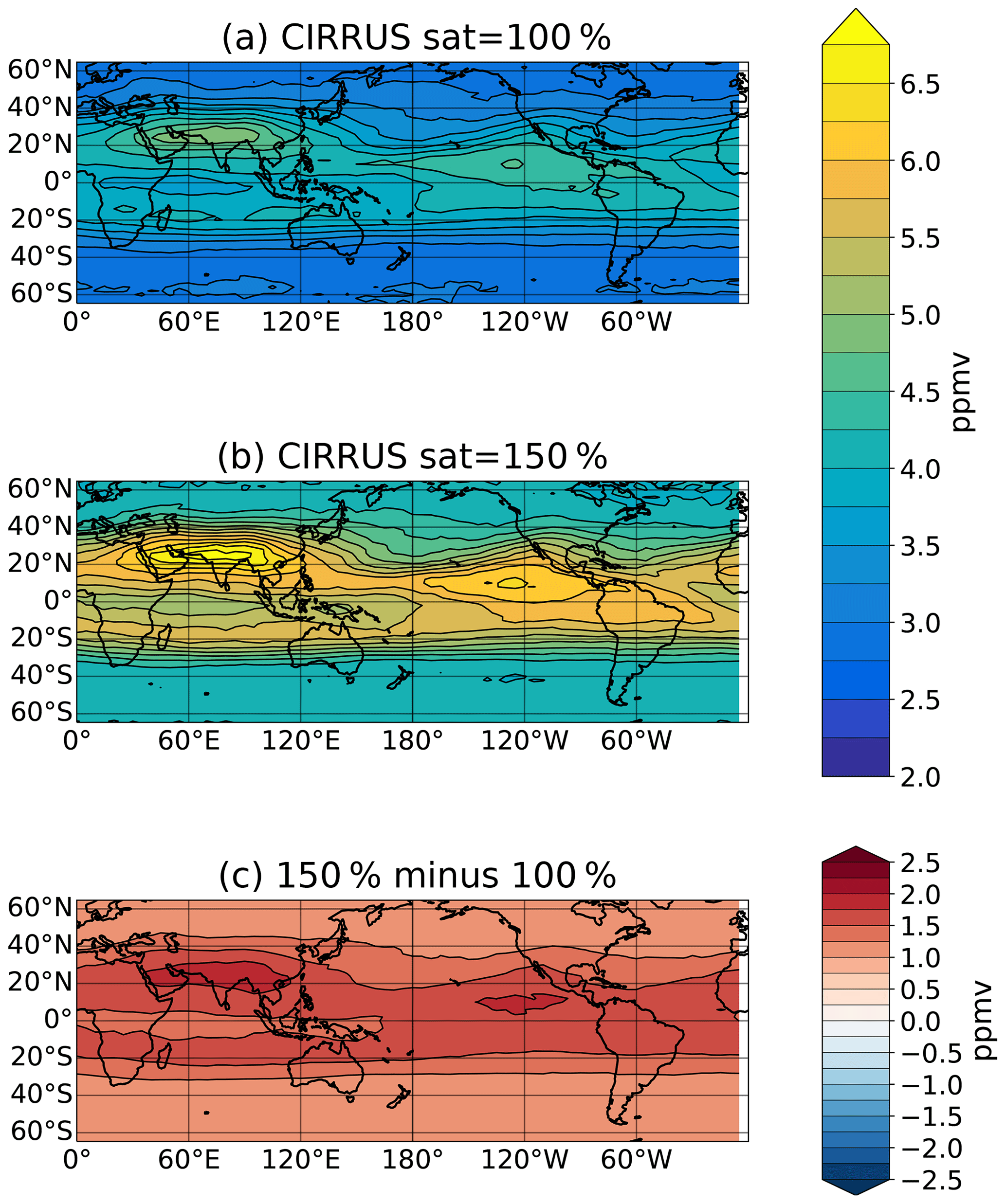
Figure 3Distribution of water vapour at 100 hPa of CIRRUS using (a) 100 % and (b) 150 % as the saturation mixing ratio with respect to ice during boreal summer for 2005–2010 and (c) their differences.
It should be kept in mind that in situ ice formation, as represented here, is only one of the many processes through which ice influences the water vapour content. Ice may be detrained in the UTLS from deep overshooting convection and evaporate afterwards, resulting in a net hydration of the UTLS (Corti et al., 2008). However, Jensen et al. (2020) concluded from observations that this effect is small, except in the NAMA, which may partly explain the poor model results there. On the other hand, convection also directly influences the vapour phase, an issue discussed in Sect. 4.1.
3.3 Variability of water vapour over monsoon regions
3.3.1 Seasonal variability
Figure 4 shows the annual cycle at 80 hPa (top) and 100 hPa (bottom) of the simulated and observed water vapour in the AMA (left column) and NAMA (right column), averaged over the period 2007–2016. For a proper comparison of the annual cycle and the peak-to-peak change between the different experiments, we have subtracted the respective April average (hereafter referred to as the offset) from each time series. April was chosen because this is when, in most experiments, the water vapour content is closest to its minimum in the AMA and NAMA.
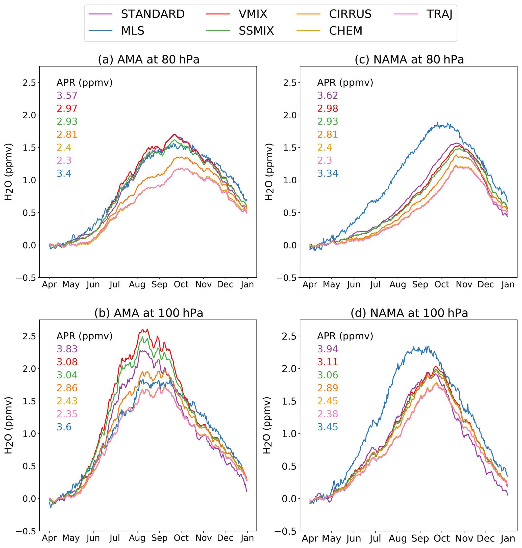
Figure 4Amplitude of the cycle of daily water vapour at (a, c) 80 hPa and (b, d) 100 hPa averaged over (a, b) the Asian Monsoon Anticyclone, AMA (20–40∘ N, 40–140∘ E), and (c, d) the North American Monsoon Anticyclone, NAMA (10–30∘ N, 220–300∘ E), for the period 2007–2016. Coloured numbers are the mean water vapour during April in each experiment, which is used as the reference level. The regions in which averages are computed correspond to the maxima of water vapour found in the boreal summer climatology of the water vapour observed by Aura MLS v4.2.
Figure 4 shows that over both the AMA and NAMA regions and at both 100 and 80 hPa, all experiments represent the observed increase in water vapour during boreal summer. The peak water vapour shows a 1–2-month delay at 80 hPa with respect to 100 hPa. Figure 4b reveals that CIRRUS, TRAJ and CHEM better represent the amplitude of the seasonal cycle of water vapour at 100 hPa in the AMA, according to MLS observations, although they underestimate the absolute value in summer (see their average for April and also Fig. 1). At 80 hPa, however, the simulations including small-scale mixing are in better agreement with MLS.
The CIRRUS experiment slightly overestimates the peak-to-peak amplitude at 100 hPa, which is about 0.3 ppmv higher than in MLS observations (Fig. 4b). CIRRUS also shows a higher offset than TRAJ and CHEM, related to a higher annual cycle minimum. Consequently, CIRRUS shows a water vapour distribution that is closer to the observations not only during the monsoon season, as shown in Fig. 1, but throughout the year, compared to TRAJ and CHEM.
Figure 4b shows a very steep water vapour increase in the AMA between June and August for SSMIX and VMIX, resulting in an overestimation of the amplitude of the annual cycle at 100 hPa (+0.8 ppmv compared to MLS and +0.9 ppmv compared to TRAJ). Furthermore, at this pressure level the differences between VMIX and SSMIX are slightly larger during the monsoon season, which is linked to the enhanced tropospheric mixing in VMIX and might be related to the impact of enhanced convective updrafts over the monsoon region during summer. Also, Fig. 4b shows that the water vapour decrease, observed from September onward, is faster in SSMIX and VMIX than in MLS observations. Thus, the good agreement between SSMIX and VMIX in the AMA during the monsoon season (Fig. 1e and f) can be attributed, on the one hand, to an increase in the minimum value over the annual cycle (as is evident from the April averages in Fig. 4b), which nevertheless remains underestimated, and on the other hand to an overestimation of the water vapour increase during the monsoon in July and August.
At 80 hPa, on the other hand, the annual cycle is better reproduced by SSMIX and VMIX than by the pure LTF models (Fig. 4a). Thus, while SSMIX and VMIX show a water vapour increase and a peak amplitude very close to the observations, the “no-mixing” experiments clearly underestimate the amplitude of the annual cycle and typically exhibit a slower water vapour increase in summer and a slight delay (1–2 weeks) of the annual maximum.
Finally, since the STANDARD experiment includes the same process parameterizations as SSMIX, it is not surprising that it also shows an overestimation of the water vapour increase in the AMA at 100 hPa, with a peak amplitude that is about 0.5 ppmv larger than in MLS (Fig. 4b). As for SSMIX and VMIX, STANDARD also results in a faster water vapour decrease from September onward at this level. However, despite very similar behaviour to SSMIX/VMIX at 80 hPa, STANDARD exhibits a weaker water vapour increase than SSMIX at 100 hPa.
Figure 4b shows that STANDARD depicts the largest offset with respect to MLS. Nevertheless, the difference in water vapour between STANDARD and MLS increases at 100 hPa during the mature phase of the AMA. This can be most likely attributed to the excessive amount of water vapour created by the small-scale mixing at the beginning of the monsoon season, as is the case for SSMIX and VMIX as well.
In the NAMA region, the annual cycle in water vapour is more consistent between the different experiments as compared to the AMA, but differences to MLS are larger (Fig. 4c and d). The increase in simulated water vapour occurs from May to September and is weaker than in MLS observations. This leads to a peak-to-peak amplitude underestimated by 0.2 to 0.4 ppmv depending on the experiment and to a delay of about 1 month to 6 weeks in the annual cycle maximum. Also, the impacts of the non-instantaneous removal of ice and of small-scale mixing in the NAMA region are quite uniform throughout the year and do not exhibit intensification during the monsoon season. This suggests a minor impact of small-scale mixing processes in the NAMA compared to the AMA. Although both SSMIX and VMIX show a wetter NAMA than CIRRUS (Fig. 1), according to Fig. 4d this is due to a uniform impact of small-scale mixing processes throughout the year rather than a peak during the monsoon season. As previously mentioned, small-scale mixing depends on deformations of the large-scale flow. The large-scale circulation of the NAMA is less confined than the AMA (Gettelman et al., 2004), which could render this region more sensitive to overshooting convection (not included in our experiments) in comparison with the AMA. Indeed, the larger and consistent differences of all model experiments to MLS also point to a significant role of convection, the common process neglected in all simulations, for moistening the NAMA. Furthermore, the STANDARD experiment shows a similar behaviour during the monsoon season, showing that the differences in the initialization scheme have a very limited influence on the annual cycle of the water vapour over the NAMA.
The annual cycle at 80 hPa (Fig. 4c) shows the lower water vapour increases, peak-to-peak amplitudes and a delayed maximum for all experiments compared to the observations. At this level, the experiments which best match the observed annual cycle are STANDARD, SSMIX, VMIX and CIRRUS, i.e. those exhibiting a higher water vapour content at 100 hPa (Fig. 1). Note that even for those experiments significant differences to MLS remain (about 0.5 ppmv).
3.3.2 Sub-seasonal variability
In order to assess the representation of water vapour variability beyond the seasonal cycle in the AMA, Fig. 5a–f depict deseasonalized daily anomalies of water vapour during 2007–2016 for each experiment and MLS observations together with the respective correlations. In order to evaluate the experiments for the entire monsoon season (from May to September, MJJAS) and the mature phase of the monsoon season (June–July–August, JJA), these correlations are computed for both periods. All LTF experiments exhibit statistically significant correlations, and the correlations tend to increase with the complexity of the experiment (i.e. the number of processes included). Thus, the simpler configurations TRAJ and CHEM have the lowest correlations of 0.51 (JJA) and 0.62 (MJJAS) (p<0.025). Note that these values are consistent with those obtained by Zhang et al. (2016) in similar experiments using ERA-Interim (their Fig. 6). Although lowest among all the experiments presented here, the still significant correlations between TRAJ (CHEM) and MLS support the idea that large-scale cold-point temperature variability is the main factor controlling water vapour variability in the Asian Monsoon UTLS, as also argued by Randel et al. (2015) and Zhang et al. (2016). Furthermore, the small difference between correlations in TRAJ and CHEM experiments reveals that methane oxidation is irrelevant to water vapour variability in the AMA.
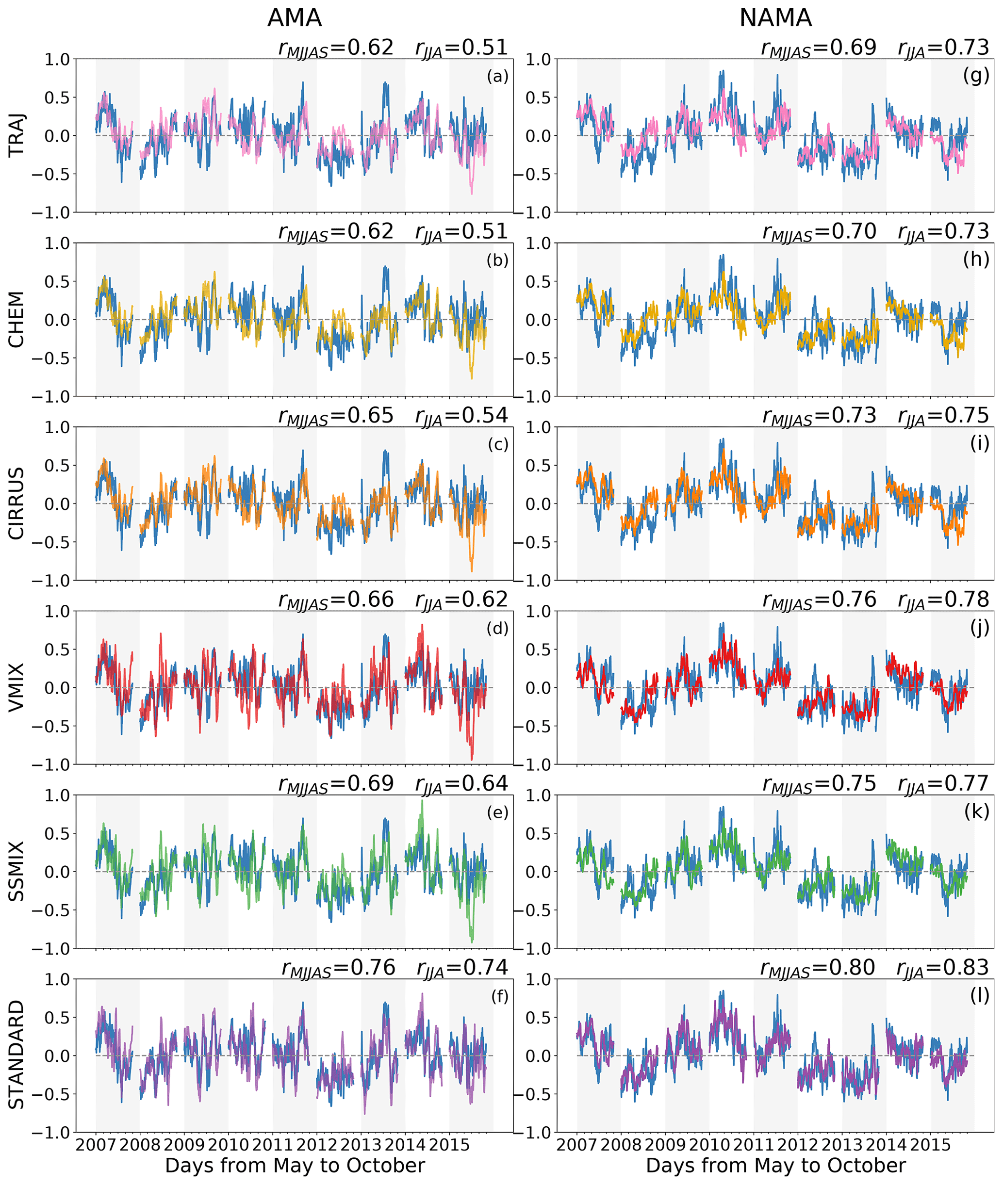
Figure 5Boreal summer deseasonalized anomalies of water vapour in (a–f) the Asian Monsoon Anticyclone, AMA, and (g–l) the North American Monsoon Anticyclone, NAMA, for (top–bottom) TRAJ, CHEM, CIRRUS, VMIX, SSMIX, and STANDARD in comparison with MLS (blue line). Correlation values between each experiment and MLS are calculated from May to September (rMJJAS) and from June to August (rJJA).
Including the simple parameterization of in situ ice formation and evaporation (CIRRUS) slightly improves the correlation during both JJA and MJJAS. This improvement is even higher when small-scale mixing processes are also included. Thus, among all LTF experiments the highest correlations are obtained for SSMIX ( for JJA/MJJAS, p<0.025) and VMIX ( for JJA/MJJAS, p<0.025). This result manifests the importance of mixing for the simulation of a realistic water vapour variability in the AMA, despite the overestimation of the water vapour increase at the beginning of the monsoon season at 100 hPa found in Fig. 4a and b. Comparing SSMIX with VMIX shows that the enhanced tropospheric mixing, which has only a mild impact on the water vapour distribution (Fig. 1f and k), does not improve the simulation of water vapour variability. Overall, the experiments including mixing do a significantly better job in simulating the sub-seasonal variability (correlations of about 0.6) than the pure LTF experiments (TRAJ, CHEM and CIRRUS, correlations with MLS slightly above 0.5). Hence, including mixing processes improves the simulation of water vapour variability in the AMA on sub-seasonal timescales. Finally, Fig. 5f shows evidence that, for both periods, the STANDARD simulation correlates best with MLS, reaching values of 0.76 and 0.74 (p<0.025) for JJA and MJJAS, and significantly improves the intra-seasonal variability in the AMA.
In the NAMA, simulated deseasonalized daily anomalies of water vapour correlate relatively well with MLS for both periods, reaching even higher correlations than in the AMA (Fig. 5g–l), despite the poor representation of the water vapour climatology in this region. The STANDARD simulation shows the highest correlation with MLS (r=0.83, p<0.025 in JJA), followed by the LTF experiments that include small-scale mixing (SSMIX, 0.77 and VMIX 0.78 in JJA). The lowest correlation is achieved by TRAJ (r=0.73 in JJA), which is still very similar to the highest correlation achieved in the AMA region. Again, the TRAJ experiment already shows high correlation with MLS, indicating that temperature is the main control factor for intra-seasonal variability also in the NAMA. The reason why correlations in the NAMA are higher than in the AMA is likely related to the fact that processes other than large-scale temperature variability play a larger role when the anticyclonic circulation and related confinement are strong enough, as in the AMA.
4.1 Convective moistening
Another important process for the UTLS water vapour budget is ice and moisture transport by convection (Dessler and Sherwood, 2004; Dessler et al., 2016). Although some of the experiments presented here include processes whose particular parameterizations may contribute to convective moistening (e.g. small-scale mixing), a direct simulation of convection is not present in these simulations.
To further investigate the additional effects of convection on the monsoon water vapour budget, we performed a modified TRAJ experiment, hereafter called CONV, in which this process is taken into account, following an approach similar to that of Ueyama et al. (2018). In CONV we use the trajectories of TRAJ to compute the LMR of the air parcels. At every time step a check is performed for whether an air parcel is located inside a cloud, i.e. at a pressure level below that of the cloud top. If this is the case, the air parcel's water vapour is set to the saturation mixing ratio (100 % relative humidity), according to the temperature that the ERA-Interim reanalysis attributes to the location of the air parcel. This process corresponds to hydration if the air parcel is initially subsaturated and dehydration if it is supersaturated (see Ueyama et al., 2018). We use ISCCP B1 (GridSat-B1) Infrared Channel Brightness Temperature combined with ERA-Interim data to determine cloud top heights (Knapp, 2014), following the methodology of Tissier and Legras (2016). Their approach is similar to the one employed by Ueyama et al. (2018) and assumes that the temperature at cloud top is equal to the temperature of the environment estimated from the reanalysis. The resulting altitude is shifted upward by 1 km to correct for biases in infrared cloud top temperature (Minnis et al., 2008). There are a few differences, however, between the two methods: first, contrary to Ueyama et al. (2018), Tissier and Legras (2016) do not distinguish convective cores from in situ formed cirrus clouds and include both for cloud top determination. The impact of this difference should be small as long as the cirrus clouds are sufficiently thin. Second, in the case of brightness temperatures lower than the local tropopause temperature, we assume that convective parcels rise adiabatically from 40 hPa below the tropopause, whereas Ueyama et al. (2018) take a mixture of tropopause (70 %) and environmental (30 %) air. Therefore, our estimated cloud top altitudes may be low biased compared to theirs. Finally, note that the ISCCP B1 has slightly lower horizontal resolution (∼8 km vs. 4 km) than the dataset of Ueyama et al. (2018) but similar temporal resolution (3-hourly). Figure 6 shows the water vapour distributions at 100 hPa of TRAJ (Fig. 6a), CONV (Fig. 6b) and the differences between both of them. The two experiments result in a very similar water vapour distribution, with a slight moistening effect caused by convection, mainly at mid and high latitudes. These results indicate that even when a convective event occurs, the water vapour is set by temperatures experienced by the air parcels after convection. This result is in agreement with Randel and Park (2006); Randel et al. (2015) but not in line with Ueyama et al. (2018). However, it should be kept in mind that Ueyama et al. (2018) focused on the analysis of a single 7 d convective event during summer 2007, whereas we consider the entire summer (June–August) for 2005–2009. Thus, while their main conclusion is that infrequent deep convection reaching above 380 K causes a strong moistening of the LS, our results show that the climatological impact of these events is likely very weak.

Figure 6Boreal summer distribution of water vapour at 100 hPa in 2008 for the (a) TRAJ and (b) CONV experiments and (c) their differences.
We have also considered only the 7 d Ueyama et al. (2018) to check whether we were able to reproduce the same results with TRAJ and CONV as their simulations without and with convection, respectively. However, in our case TRAJ produces a maximum of water vapour in the AMA that is not observed in their non-convective experiment. This suggests that there are additional features, further than the differences mentioned before, that make the comparison between the experiments in Ueyama et al. (2018) and ours difficult. Another limitation of our approach in CONV is that we have not taken into account the role of convective ice. According to Wang et al. (2019), the main impact of convection on the LS water vapour occurs through the injection of ice. The latter assertion, however, is contrary to the conclusions of Ueyama et al. (2018). These differences between the different studies highlight the large existing uncertainty about the role of convection for LS water vapour. A deeper analysis of this issue should be considered in future studies.
4.2 Sensitivity of water vapour to the LTF set-up
In the LTF experiments previously described, we have used the same longitude–latitude grid to release new air parcels at the same initial potential temperature of 360 K. This configuration, which has been chosen following the procedure of Schoeberl and Dessler (2011), might have an effect on our results. In fact, Schoeberl et al. (2013) and Wang et al. (2019) use 370 K as the initial potential temperature level for air parcels released in the Asian Monsoon region. They argue that because the LZRH is higher over the AMA than in other regions, many air parcels released at 360 K may descend and are removed from the simulation. Figure 7a shows the normalized distribution of air parcels in TRAJ at 100 hPa centered in the AMA for JJA in 2007. As we could expect from Schoeberl et al. (2013) and Wang et al. (2019), the AMA is characterized by a lower density of air parcels. Because a low number of air parcels could condition the robustness of the results, this raises the question of the possible impact of the number of air parcels in the AMA on the water vapour distribution in this region. To test this potential sensitivity to the number of air parcels, we have performed two additional TRAJ experiments in which either the number of air parcels newly released has been increased (TRAJ-denser) or the initial potential temperature (TRAJ-370 K) has been changed. In TRAJ-denser the number of air parcels is increased by releasing them on a higher-resolution grid (2.5∘ longitude × 1∘ latitude). By contrast, in TRAJ-370 K the initialization grid maintains the same resolution as in TRAJ, but air parcels are launched at the θ=370 K surface instead of at 360 K.

Figure 7(a) Normalized density of air parcels in the AMA region during JJA in 2007 for the TRAJ experiment. Distributions of the relative number of air parcels with respect to TRAJ in (b) TRAJ-denser and (c) TRAJ-370 K. Boreal water vapour distributions of (d) TRAJ, (e) TRAJ-denser and (d) TRAJ-370 K in 2007.
Figure 7b and c show the relative number of air parcels in the AMA at 100 hPa of TRAJ-denser and TRAJ-370 K with respect to TRAJ. In addition, Fig. 7d–f show the water vapour distributions of TRAJ, TRAJ-denser and TRAJ-370 K for the same season and year. In both experiments, the density of air parcels has increased notably with respect to TRAJ. There are 4 times more air parcels in TRAJ-denser (Fig. 7b) and 2 times more in TRAJ-370 K (Fig. 7c) than in TRAJ. As in TRAJ-denser more air parcels are released inside the AMA, a larger number of them reach the 100 hPa level. However, this larger number of air parcels is not accompanied by an enhancement of water vapour (Fig. 7e). Therefore, we conclude that increasing the resolution of the initialization grid used in our LTF experiments does not have an impact on our results, which means that the resolution and particle number of the TRAJ experiment are high enough to adequately capture the spatial variability of the temperature field and its impact on water vapour. By contrast, TRAJ-370 K exhibits a moister water vapour distribution in the AMA than the original TRAJ experiment (Fig. 7f). This might be explained by the fact that the AMA shows a stronger anticyclonic circulation at 370 K than at 360 K (Bergman et al., 2013), giving rise to the uplift of more air parcels through the inner core of the AMA. The stronger confinement of this region can allow a greater number of air parcels to avoid the coldest regions, which are located at the south-eastern flank of the AMA. Thus, when the air parcels spawn to other regions at the 100 hPa level due to the weakening of the anticyclone circulation, they transport a larger water vapour content than air parcels reaching the same pressure level in TRAJ. This widening of the vertical transport conduit of air parcels when being uplifted in the Asian Monsoon Anticyclone is consistent with the main transport pathway proposed by Bergman et al. (2013).
These results show that our LTF experiments have a sufficient number of air parcels to be statistically significant. Furthermore, they point out that the selection of a higher initial potential temperature in the AMA has an impact on water vapour distributions, likely related to the larger exposure of the chosen potential temperature level to stronger confinement in the AMA. Thus, we conclude that the selection of the initial potential temperature should not only take into account the level of zero radiative heating, but also the strength and confinement of the AMA.
These sensitivity tests of the domain-filling technique to a different selection of arbitrarily chosen parameters do not cover possible impacts of the LTF scheme itself in our water vapour results. To study this we compare a LTF experiment, SSMIX, with a non-LTF experiment, STANDARD. Despite the similar set of parameterizations included, the STANDARD and SSMIX experiments significantly differ, and STANDARD agrees better with MLS regarding seasonal and intra-seasonal variability in the AMA and NAMA. The remaining discrepancies might be due to (i) the initial water vapour content of the air parcels and (ii) the filtering of air parcels below 250 hPa and above 1800 K, in particular the absence of a troposphere.
To test point (i), we performed an additional experiment configured as SSMIX but doubling the initial water vapour content of air parcels from 50 to 100 ppmv. Figure A3 in the Appendix shows that the distribution at 100 hPa is not affected by this change in the initial condition. Note however that this does not suggest that the water vapour is entirely insensitive to the lower boundary condition, as explained below.
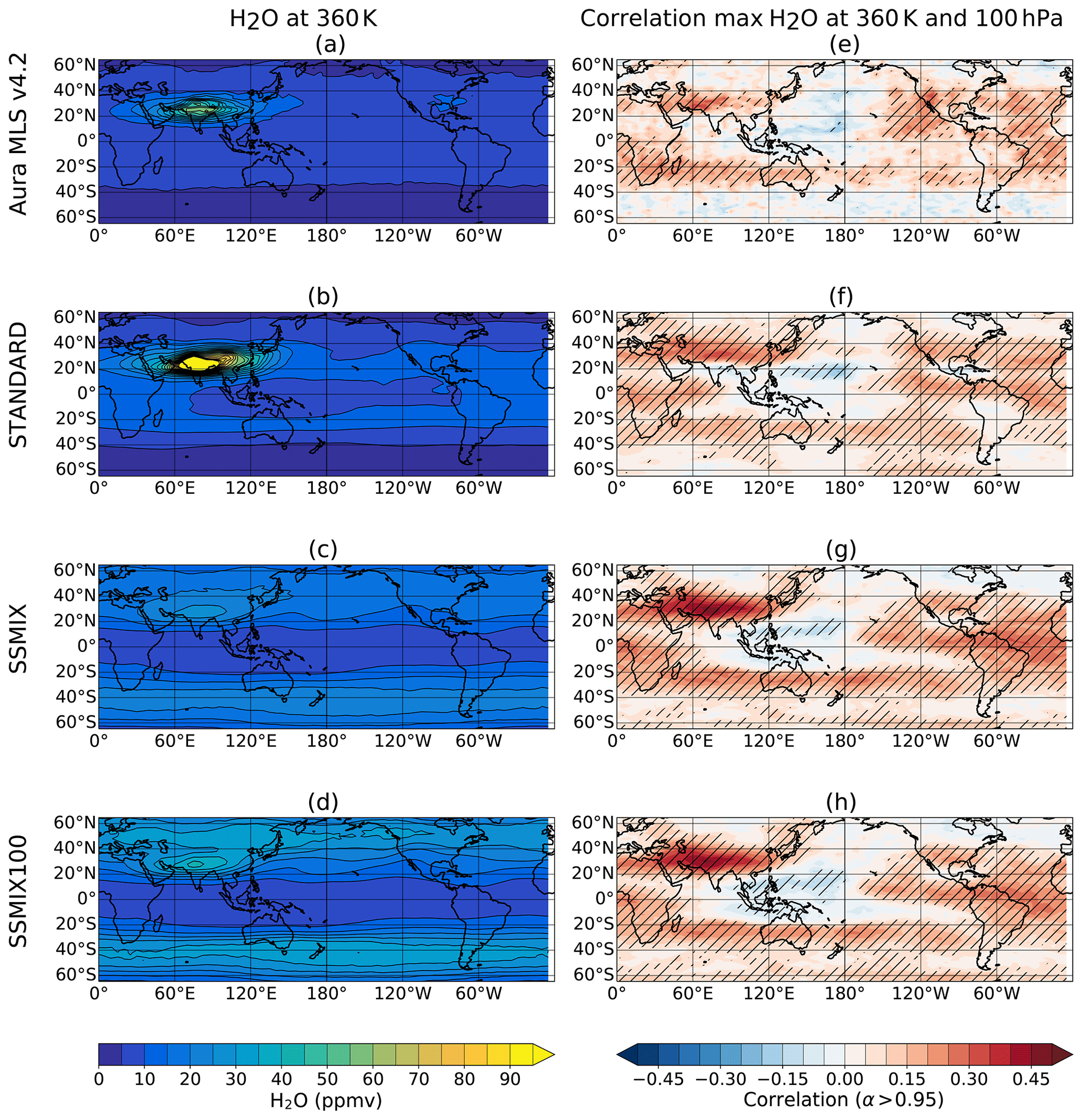
Figure 8(a–d) Climatology of water vapour at 360 K from (a) Aura MLS v4.2 observations, (b) STANDARD, (c) SSMIX and (d) SSMIX initialized with 100 ppmv. (e–h) Correlation between the water vapour time series averaged in 60–100∘ E, 20–30∘ N at 360 K and the time series of water vapour at 100 hPa at each grid point during boreal summer for (e) Aura MLS v4.2 (f) STANDARD, (g) SSMIX and (h) SSMIX initialized with 100 ppmv.
In order to further investigate this result, Fig. 8 depicts the 360 K water vapour maps (corresponding to the level of initialization of SSMIX) for MLS observations, STANDARD and the two SSMIX experiments. Note that the water vapour mixing ratio in the SSMIX is significantly lower than the initialization value. This is due to the presence of older air parcels which have been released at earlier time steps, have undergone dehydration and have been transported into the 360 K layer from above. This stagnation and return of old air parcels is allowed as the filtering occurs at 250 hPa, which is below the initialization level. Therefore, we conclude that the initialization value in LTF experiments cannot be considered a lower boundary condition for LTF simulations in the Asian Monsoon.
It turns out that the water vapour variability at 100 hPa is, indeed, sensitive to this lower boundary condition. This is indicated by the high correlations between the water vapour at 360 K in the AMA region and local H2O at 100 hPa (Fig. 8e–h), which peak over the Asian Monsoon. The significantly different lower boundary conditions shown in (Fig. 8a–d) thus likely cause parts of the observed differences between STANDARD and SSMIX at 100 hPa. In the standard LTF approach, this boundary condition is not directly set because of the mixture of old and young air parcels making up the air masses at 360 K.
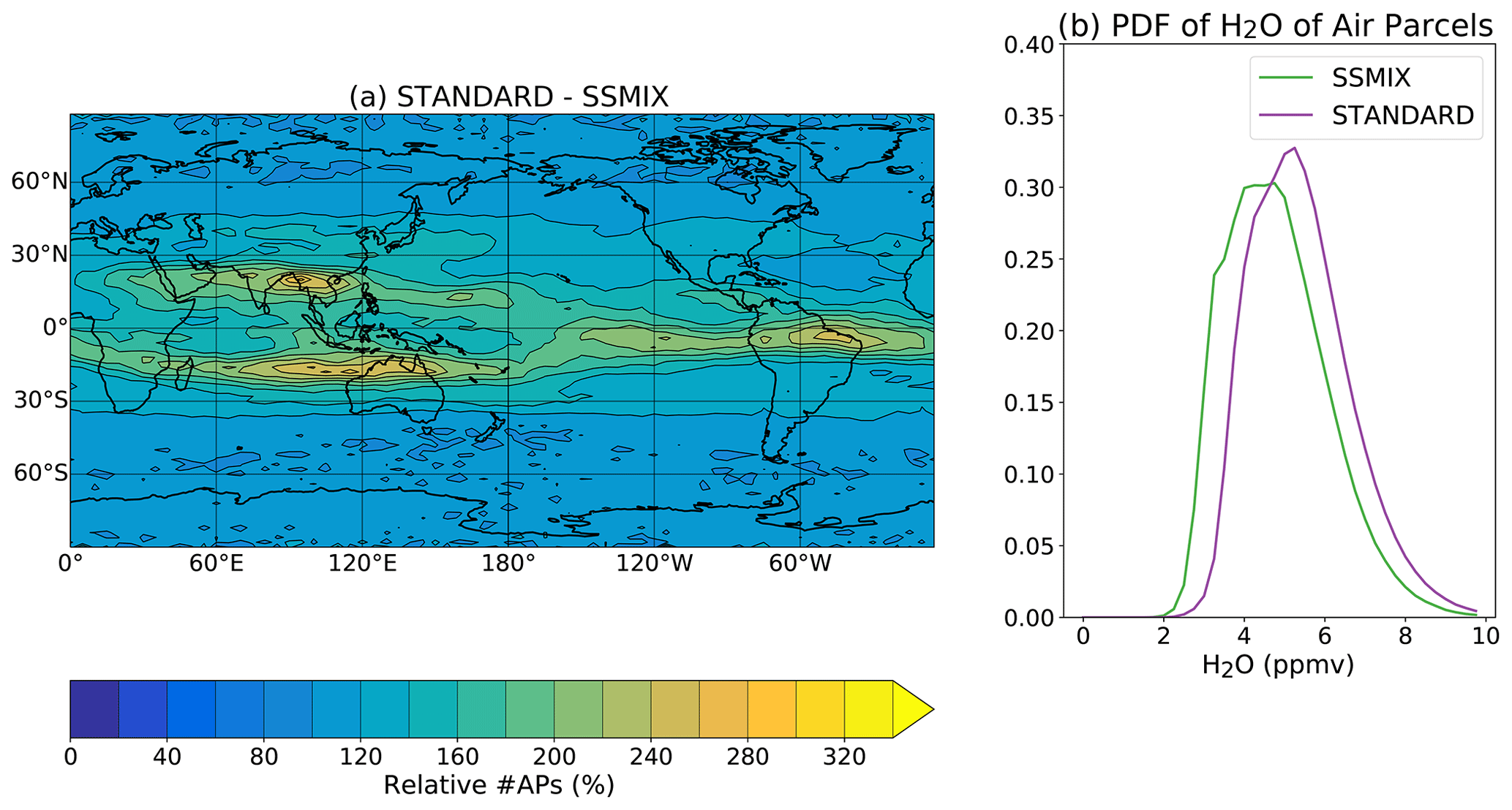
Figure 9(a) Distribution of the relative number of air parcels simulated in STANDARD with respect to SSMIX during JJA for 2007–2016. (b) Normalized PDF of the water vapour of air parcels encountered during JJA (2007–2016) over the Asian Monsoon region (20–40∘ N, 40–140∘ E) for SSMIX and STANDARD.
While this issue may be interpreted as a too dry lower boundary condition, it is in the end related to missing transport pathways in the lower part of the simulated domain. This interpretation is supported by Fig. 9a, which shows the relative percentage of air parcels simulated in STANDARD with respect to SSMIX. STANDARD shows a higher number of air parcels than SSMIX throughout the domain, and in particular in the AMA and the Southern Hemisphere subtropics (Fig. 9a). Not only does STANDARD simulate more air parcels in the AMA, but these parcels are also wetter, as shown in the probability density function (PDF) of the water vapour content of the air parcels (Fig. 9b). These differences suggest a lack of vertical transport of moist tropospheric air parcels from lower levels in the LTF initialization (where these air parcels are removed). Besides vertical transport, it is likely that inhibited horizontal entrainment also plays a role, since at the 360 K initialization level the inner anticyclone core is, to some degree, isolated from the surrounding areas, as shown in Garny and Randel (2016).
In this study, we compared numerical Lagrangian transport simulations based on the forward domain-filling technique developed by Schoeberl and Dessler (2011) with the CLaMS model (McKenna et al., 2002b, a) in order to assess the impact of methane oxidation, ice microphysics, small-scale mixing and enhanced tropospheric mixing on the water vapour distribution in the lower stratosphere during boreal summer. A particular focus was laid on the Asian (AMA) and North American (NAMA) Monsoon Anticyclones in the UTLS.
In agreement with previous work (e.g. James et al., 2008; Schoeberl and Dessler, 2011), we find that simple last-dehydration-point LTF modelling based on large-scale reanalysis temperature and wind fields can qualitatively reproduce the water vapour signal in the AMA and its variability but with simulated mixing ratios dry-biased. Furthermore, while our modelling set-up reproduces well the water vapour signal in the AMA, the location and amplitude of the NAMA maximum are less well reproduced.
While the effect of methane oxidation is small, a simplified representation of ice microphysics significantly moistens the LS. The magnitude of the water vapour enhancement largely depends on microphysical assumptions. A new finding of our study is that small-scale mixing processes, as parameterized in CLaMS depending on shear in the large-scale flow, has a strong impact on water vapour in the AMA region. A sensitivity simulation evaluating convective hydration suggests that its pattern is different from that of small-scale mixing and not particularly strong in the AMA, which tends to confirm the distinct signature of mixing. Interestingly, we find that the impact of changing microphysical assumptions also varies depending on the presence of mixing. This suggests that mixing is an important process for understanding boreal summer water vapour. For a more complete picture of the UTLS boreal summer water vapour budget, future research should focus on investigating the impact of mixing on water vapour isotopes and high-altitude cloud cover.
This hypothetical situation is illustrated in Fig. A1. Given two air parcels, “A” and “B”, at different altitudes but close enough, they mix together into “C”. In case C is supersaturated after mixing, the microphysics of ice turns it into saturation, forming ice particles with the excess water vapour. However, this saturation value would be higher than that corresponding to the minimum temperature in the vertical profile considered, Tmin. Therefore, the water vapour of C would not be set by Tmin, but by the temperature at its altitude. In case Tmin represents the temperature of the CPT, then water vapour has been transported to higher altitudes, avoiding the CPT and giving rise to an increase in water vapour over most regions, but especially where the mixing is stronger.

Figure A1Hypothetical scheme in which the mixing process avoids a “cold trap”. Air parcels A and B mix into C. Due to the temperature vertical profile, temperature in C is larger than the temperature registered below, Tmin. Therefore, in case C is saturated according to its temperature, the water vapour content would be larger than if an air parcel would be transported to the same altitude encountering Tmin.

Figure A2Differences in the distribution of water vapour at 100 hPa between VMIX (experiment with ice microphysics) and VMIXnocirrus (experiment without ice microphysics) during JJA for 2005–2008. Red colours mean VMIX performs larger water vapour than VMIXnocirrus.
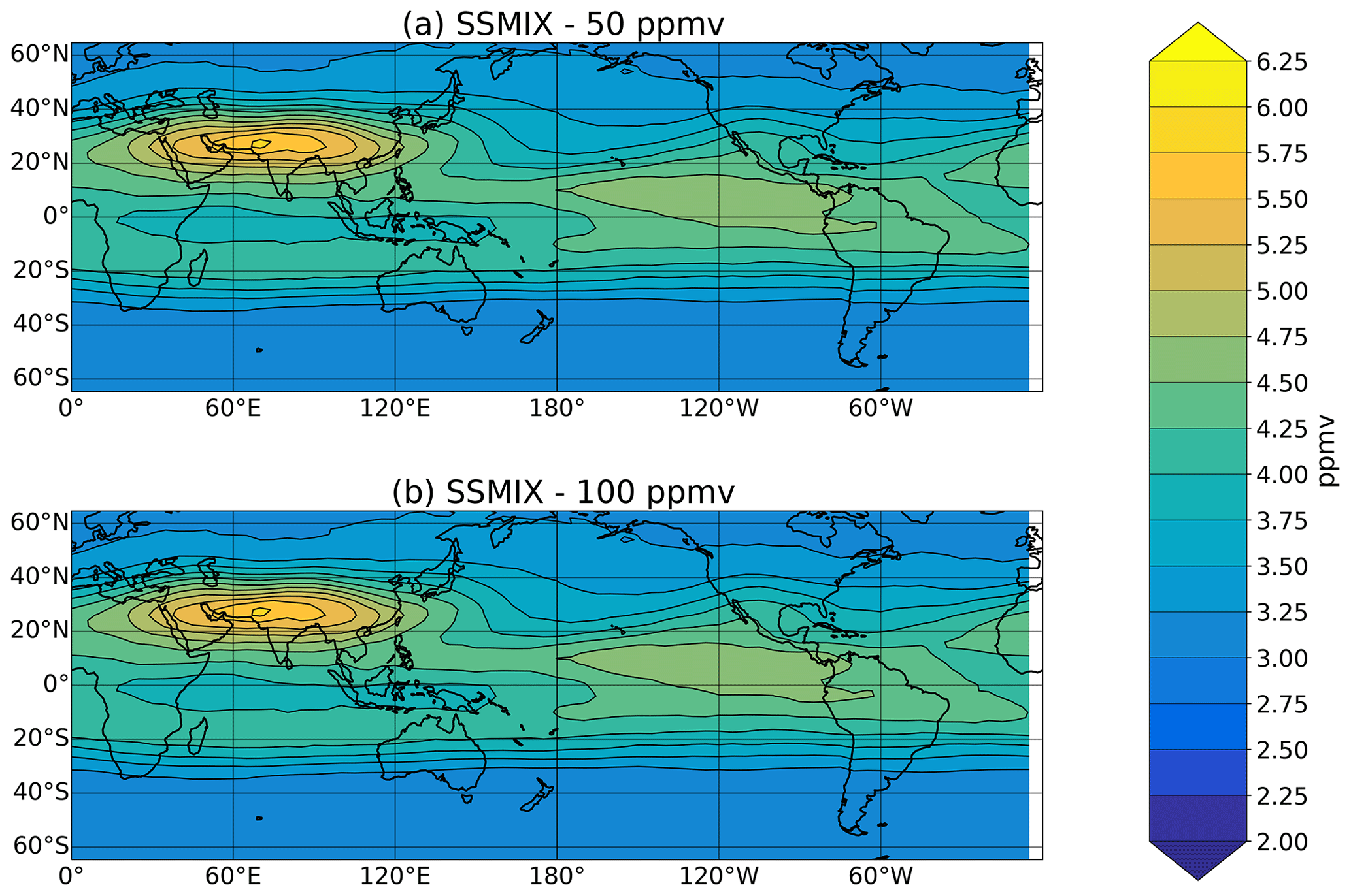
Figure A3Distribution of water vapour at 100 hPa of SSMIX initialized with (a) 50 ppmv and (b) 100 ppmv during boreal summer for 2007–2016.
Data used for experiments are available upon request from authors Nuria Pilar Plaza (npplamar@upo.es) and Felix Ploeger (fploeger@fz.julich.de). MLS H2O version 4.2 data can be obtained from the MLS website https://mls.jpl.nasa.gov/data/v4-2_data_quality_document.pdf (Livesey et al., 2018).
NPP, AP and FP designed the experiments. NPP and AP performed the experiments with CLaMS. NPP performed the data analysis. NPP, CPO, AP and FP contributed to the discussion of results. NPP and CPO wrote the text. CPO, AP and FP made the final review.
The authors declare that they have no conflict of interest.
Publisher's note: Copernicus Publications remains neutral with regard to jurisdictional claims in published maps and institutional affiliations.
We would like to thank Bernard Legras for performing an experiment with TRACZILLA and sharing with us his work. We thank the Institute of Climate from the Research Center of Jülich and, especially, Martin Riese, for their scientific, technical and financial support.
This research has been supported by the Spanish Ministerio de Economía y Competitividad (grant no. CGL2016-78562-P).
This paper was edited by Jianzhong Ma and reviewed by two anonymous referees.
Bergman, J. W., Fierli, F., Jensen, E. J., Honomichl, S., and Pan, L. L.: Boundary layer sources for the Asian anticyclone: Regional contributions to a vertical conduit, J. Geophys. Res.-Atmos., 118, 2560–2575, 2013. a, b
Corti, T., Luo, B. P., de Reus, M., Brunner, D., Cairo, F., Mahoney, M. J., Martucci, G., Matthey, R., Mitev, V., dos Santos, F. H., Schiller, C., Shur, G., Sitnikov, N. M., Spelten, N., Vössing, H. J., Borrmann, S., and Peter, T.: Unprecedented evidence for deep convection hydrating the tropical stratosphere, Geophys. Res. Lett., 35, L10810, https://doi.org/10.1029/2008GL033641, 2008. a, b, c
Dee, D. P., Uppala, S. M., Simmons, A. J., Berrisford, P., Poli, P., Kobayashi, S., Andrae, U., Balmaseda, M. A., Balsamo, G., Bauer, P., Bechtold, P., Beljaars, A. C. M., van de Berg, L., Bidlot, J., Bormann, N., Delsol, C., Dragani, R., Fuentes, M., Geer, A. J., Haimberger, L., Healy, S. B., Hersbach, H., Hólm, E. V., Isaksen, L., Kållberg, P., Köhler, M., Matricardi, M., McNally, A. P., Monge-Sanz, B. M., Morcrette, J.-J., Park, B.-K., Peubey, C., de Rosnay, P., Tavolato, C., Thépaut, J.-N., and Vitart, F.: The ERA-Interim reanalysis: Configuration and performance of the data assimilation system, Q. J. Roy. Meteor. Soc., 137, 553–597, 2011. a
Dessler, A. and Sherwood, S.: Effect of convection on the summertime extratropical lower stratosphere, J. Geophys. Res.-Atmos., 109, D23301, https://doi.org/10.1029/2004JD005209, 2004. a, b, c
Dessler, A., Hanisco, T., and Fueglistaler, S.: Effects of convective ice lofting on H2O and HDO in the tropical tropopause layer, J. Geophys. Res.-Atmos., 112, D18309, https://doi.org/10.1029/2007JD008609, 2007. a, b
Dessler, A., Schoeberl, M., Wang, T., Davis, S., Rosenlof, K., and Vernier, J.-P.: Variations of stratospheric water vapor over the past three decades, J. Geophys. Res.-Atmos., 119, 12–588, 2014. a
Dessler, A., Ye, H., Wang, T., Schoeberl, M., Oman, L., Douglass, A., Butler, A., Rosenlof, K., Davis, S., and Portmann, R.: Transport of ice into the stratosphere and the humidification of the stratosphere over the 21st century, Geophys. Res. Lett., 43, 2323–2329, 2016. a, b
Diallo, M., Riese, M., Birner, T., Konopka, P., Müller, R., Hegglin, M. I., Santee, M. L., Baldwin, M., Legras, B., and Ploeger, F.: Response of stratospheric water vapor and ozone to the unusual timing of El Niño and the QBO disruption in 2015–2016, Atmos. Chem. Phys., 18, 13055–13073, https://doi.org/10.5194/acp-18-13055-2018, 2018. a, b, c, d
Dinh, T., Podglajen, A., Hertzog, A., Legras, B., and Plougonven, R.: Effect of gravity wave temperature fluctuations on homogeneous ice nucleation in the tropical tropopause layer, Atmos. Chem. Phys., 16, 35–46, https://doi.org/10.5194/acp-16-35-2016, 2016. a
Fueglistaler, S. and Baker, M. B.: A modelling study of the impact of cirrus clouds on the moisture budget of the upper troposphere, Atmos. Chem. Phys., 6, 1425–1434, https://doi.org/10.5194/acp-6-1425-2006, 2006. a
Fueglistaler, S. and Haynes, P.: Control of interannual and longer-term variability of stratospheric water vapor, J. Geophys. Res.-Atmos., 110, D24108, https://doi.org/10.1029/2005JD006019, 2005. a, b, c
Fueglistaler, S., Bonazzola, M., Haynes, P., and Peter, T.: Stratospheric water vapor predicted from the Lagrangian temperature history of air entering the stratosphere in the tropics, J. Geophys. Res.-Atmos., 110, D08107, https://doi.org/10.1029/2004JD005516, 2005. a
Fueglistaler, S., Legras, B., Beljaars, A., Morcrette, J.-J., Simmons, A., Tompkins, A., and Uppala, S.: The diabatic heat budget of the upper troposphere and lower/mid stratosphere in ECMWF reanalyses, Q. J. Roy. Meteor. Soc., 135, 21–37, 2009. a
Garny, H. and Randel, W. J.: Transport pathways from the Asian monsoon anticyclone to the stratosphere, Atmos. Chem. Phys., 16, 2703–2718, https://doi.org/10.5194/acp-16-2703-2016, 2016. a
Gettelman, A., Randel, W., Wu, F., and Massie, S.: Transport of water vapor in the tropical tropopause layer, Geophys. Res. Lett., 29, 9-1–9-4, https://doi.org/10.1029/2001GL013818, 2002a. a, b, c
Gettelman, A., Salby, M., and Sassi, F.: Distribution and influence of convection in the tropical tropopause region, J. Geophys. Res.-Atmos., 107, ACL 6-1–ACL 6-12, https://doi.org/10.1029/2001JD001048, 2002b. a
Gettelman, A., Kinnison, D. E., Dunkerton, T. J., and Brasseur, G. P.: Impact of monsoon circulations on the upper troposphere and lower stratosphere, J. Geophys. Res.-Atmos., 109, D22101, https://doi.org/10.1029/2004JD004878, 2004. a, b
Gill, A. E.: Some simple solutions for heat-induced tropical circulation, Q. J. Roy. Meteor. Soc., 106, 447–462, 1980. a
Hoskins, B. J. and Rodwell, M. J.: A model of the Asian summer monsoon. Part I: The global scale, J. Atmos. Sci., 52, 1329–1340, 1995. a
James, R., Bonazzola, M., Legras, B., Surbled, K., and Fueglistaler, S.: Water vapor transport and dehydration above convective outflow during Asian monsoon, Geophys. Res. Lett., 35, L20810, https://doi.org/10.1029/2008GL035441, 2008. a, b, c
Jensen, E. and Pfister, L.: Transport and freeze-drying in the tropical tropopause layer, J. Geophys. Res.-Atmos., 109, D02207, https://doi.org/10.1029/2003JD004022, 2004. a, b
Jensen, E. J., Ueyama, R., Pfister, L., Bui, T. V., Alexander, M. J., Podglajen, A., Hertzog, A., Woods, S., Lawson, R. P., Kim, J.-E., and Schoeberl, M. R.: High-frequency gravity waves and homogeneous ice nucleation in tropical tropopause layer cirrus, Geophys. Res. Lett., 43, 6629–6635, https://doi.org/10.1002/2016GL069426, 2016. a
Jensen, E. J., Pan, L. L., Honomichl, S., Diskin, G. S., Krämer, M., Spelten, N., Günther, G., Hurst, D. F., Fujiwara, M., Vömel, H., Selkirk, H. B., Suzuki, J., Schwartz, M. J., and Smith, J. B.: Assessment of Observational Evidence for Direct Convective Hydration of the Lower Stratosphere, J. Geophys. Res.-Atmos., 125, e2020JD032793, https://doi.org/10.1029/2020JD032793, 2020. a
Kim, J., Randel, W. J., and Birner, T.: Convectively driven tropopause-level cooling and its influences on stratospheric moisture, J. Geophys. Res.-Atmos., 123, 590–606, 2018. a
Knapp, K.: NOAA Climate Data Record (CDR) of Gridded Satellite Data from ISCCP B1 (GridSat-B1) Infrared Channel Brightness Temperature, Version 2, NOAA's CDR Program, https://doi.org/10.7289/V59P2ZKR, 2014. a
Konopka, P. and Pan, L. L.: On the mixing-driven formation of the Extratropical Transition Layer (ExTL), J. Geophys. Res.-Atmos., 117, D18301, https://doi.org/10.1029/2012JD017876, 2012. a
Konopka, P., Steinhorst, H.-M., Grooß, J.-U., Günther, G., Müller, R., Elkins, J. W., Jost, H.-J., Richard, E., Schmidt, U.,Toon, G., and McKenna, D. S.: Mixing and ozone loss in the 1999–2000 Arctic vortex: Simulations with the three-dimensional Chemical Lagrangian Model of the Stratosphere (CLaMS), J. Geophys. Res.-Atmos., 109, D02315, https://doi.org/10.1029/2003JD003792, 2004. a, b, c, d, e, f
Konopka, P., Günther, G., Müller, R., dos Santos, F. H. S., Schiller, C., Ravegnani, F., Ulanovsky, A., Schlager, H., Volk, C. M., Viciani, S., Pan, L. L., McKenna, D.-S., and Riese, M.: Contribution of mixing to upward transport across the tropical tropopause layer (TTL), Atmos. Chem. Phys., 7, 3285–3308, https://doi.org/10.5194/acp-7-3285-2007, 2007. a, b, c, d
Konopka, P., Tao, M., Ploeger, F., Diallo, M., and Riese, M.: Tropospheric mixing and parametrization of unresolved convective updrafts as implemented in the Chemical Lagrangian Model of the Stratosphere (CLaMS v2.0), Geosci. Model Dev., 12, 2441–2462, https://doi.org/10.5194/gmd-12-2441-2019, 2019. a, b
Krämer, M., Schiller, C., Afchine, A., Bauer, R., Gensch, I., Mangold, A., Schlicht, S., Spelten, N., Sitnikov, N., Borrmann, S., de Reus, M., and Spichtinger, P.: Ice supersaturations and cirrus cloud crystal numbers, Atmos. Chem. Phys., 9, 3505–3522, https://doi.org/10.5194/acp-9-3505-2009, 2009. a, b
Krämer, M., Rolf, C., Spelten, N., Afchine, A., Fahey, D., Jensen, E., Khaykin, S., Kuhn, T., Lawson, P., Lykov, A., Pan, L. L., Riese, M., Rollins, A., Stroh, F., Thornberry, T., Wolf, V., Woods, S., Spichtinger, P., Quaas, J., and Sourdeval, O.: A microphysics guide to cirrus – Part 2: Climatologies of clouds and humidity from observations, Atmos. Chem. Phys., 20, 12569–12608, https://doi.org/10.5194/acp-20-12569-2020, 2020. a, b, c, d
Lambert, A., Read, W., and Livesey, N.: MLS/Aura Level 2 Water Vapor (H2O) Mixing Ratio V004, Goddard Earth Sciences Data and Information Services Center (GES DISC), Greenbelt, MD, USA, 2015. a
Livesey, N., Read, W., Wagner, P., Froidevaux, L., Lambert, A., Manney, G., Millán Valle, L., Pumphrey, H., Santee, M., Schwartz, M., Wang, S., Fuller, R., Jarnot, R., Knosp, B., Martinez, E., and Lay, R.: Version 4.2 × Level 2 data quality and description document, Jet Propul, Tech. rep., Lab., Tech. Rep. JPL D-33509 Rev. D, Pasadena, CA, USA, available at: https://mls.jpl.nasa.gov/data/v4-2_data_quality_document.pdf (last access: 21 June 2021), 2018. a, b
Marti, J. and Mauersberger, K.: A survey and new measurements of ice vapor pressure at temperatures between 170 and 250 K, Geophys. Res. Lett., 20, 363–366, 1993. a
McKenna, D. S., Grooß, J.-U., Günther, G., Konopka, P., Müller, R., Carver, G., and Sasano, Y.: A new Chemical Lagrangian Model of the Stratosphere (CLaMS) 2. Formulation of chemistry scheme and initialization, J. Geophys. Res.-Atmos., 107, ACH 4-1–ACH 4-14, https://doi.org/10.1029/2000JD000113, 2002a. a, b, c
McKenna, D. S., Konopka, P., Grooß, J.-U., Günther, G., Müller, R., Spang, R., Offermann, D., and Orsolini, Y.: A new Chemical Lagrangian Model of the Stratosphere (CLaMS) 1. Formulation of advection and mixing, J. Geophys. Res.-Atmos., 107, ACH 15-1–ACH 15-15, https://doi.org/10.1029/2000JD000114, 2002b. a, b, c, d, e
Minnis, P., Yost, C. R., Sun-Mack, S., and Chen, Y.: Estimating the top altitude of optically thick ice clouds from thermal infrared satellite observations using CALIPSO data, Geophys. Res. Lett., 35, L12801, https://doi.org/10.1029/2008GL033947, 2008. a
Mote, P. W., Rosenlof, K. H., McIntyre, M. E., Carr, E. S., Gille, J. C., Holton, J. R., Kinnersley, J. S., Pumphrey, H. C., Russell III, J. M., and Waters, J. W.: An atmospheric tape recorder: The imprint of tropical tropopause temperatures on stratospheric water vapor, J. Geophys. Res.-Atmos., 101, 3989–4006, 1996. a, b
Murphy, D. M. and Koop, T.: Review of the vapour pressures of ice and supercooled water for atmospheric applications, Q. J. Roy. Meteor. Soc., 131, 1539–1565, 2005. a, b
Nützel, M., Podglajen, A., Garny, H., and Ploeger, F.: Quantification of water vapour transport from the Asian monsoon to the stratosphere, Atmos. Chem. Phys., 19, 8947–8966, https://doi.org/10.5194/acp-19-8947-2019, 2019. a
Pan, L., Konopka, P., and Browell, E.: Observations and model simulations of mixing near the extratropical tropopause, J. Geophys. Res.-Atmos., 111, D05106, https://doi.org/10.1029/2005JD006480, 2006. a, b
Park, M., Randel, W. J., Gettelman, A., Massie, S. T., and Jiang, J. H.: Transport above the Asian summer monsoon anticyclone inferred from Aura Microwave Limb Sounder tracers, J. Geophys. Res.-Atmos., 112, D16309, https://doi.org/10.1029/2006JD008294, 2007. a, b, c
Ploeger, F., Konopka, P., Günther, G., Grooß, J.-U., and Müller, R.: Impact of the vertical velocity scheme on modeling transport in the tropical tropopause layer, J. Geophys. Res.-Atmos., 115, D03301, https://doi.org/10.1029/2009JD012023, 2010. a
Ploeger, F., Günther, G., Konopka, P., Fueglistaler, S., Müller, R., Hoppe, C., Kunz, A., Spang, R., Grooß, J.-U., and Riese, M.: Horizontal water vapor transport in the lower stratosphere from subtropics to high latitudes during boreal summer, J. Geophys. Res.-Atmos., 118, 8111–8127, 2013. a, b, c, d, e, f, g
Ploeger, F., Gottschling, C., Griessbach, S., Grooß, J.-U., Guenther, G., Konopka, P., Müller, R., Riese, M., Stroh, F., Tao, M., Ungermann, J., Vogel, B., and von Hobe, M.: A potential vorticity-based determination of the transport barrier in the Asian summer monsoon anticyclone, Atmos. Chem. Phys., 15, 13145–13159, https://doi.org/10.5194/acp-15-13145-2015, 2015. a
Ploeger, F., Konopka, P., Walker, K., and Riese, M.: Quantifying pollution transport from the Asian monsoon anticyclone into the lower stratosphere, Atmos. Chem. Phys., 17, 7055–7066, https://doi.org/10.5194/acp-17-7055-2017, 2017. a
Podglajen, A., Hertzog, A., Plougonven, R., and Legras, B.: Lagrangian temperature and vertical velocity fluctuations due to gravity waves in the lower stratosphere, Geophys. Res. Lett., 43, 3543–3553, https://doi.org/10.1002/2016GL068148, 2016. a
Podglajen, A., Bui, T. P., Dean-Day, J. M., Pfister, L., Jensen, E. J., Alexander, M. J., Hertzog, A., Kärcher, B., Plougonven, R., and Randel, W. J.: Small-scale wind fluctuations in the tropical tropopause layer from aircraft measurements: Occurrence, nature, and impact on vertical mixing, J. Atmos. Sci., 74, 3847–3869, 2017. a
Pommrich, R., Müller, R., Grooß, J.-U., Konopka, P., Ploeger, F., Vogel, B., Tao, M., Hoppe, C. M., Günther, G., Spelten, N., Hoffmann, L., Pumphrey, H.-C., Viciani, S., D'Amato, F., Volk, C. M., Hoor, P., Schlager, H., and Riese, M.: Tropical troposphere to stratosphere transport of carbon monoxide and long-lived trace species in the Chemical Lagrangian Model of the Stratosphere (CLaMS), Geosci. Model Dev., 7, 2895–2916, https://doi.org/10.5194/gmd-7-2895-2014, 2014. a, b
Poshyvailo, L., Müller, R., Konopka, P., Günther, G., Riese, M., Podglajen, A., and Ploeger, F.: Sensitivities of modelled water vapour in the lower stratosphere: temperature uncertainty, effects of horizontal transport and small-scale mixing, Atmos. Chem. Phys., 18, 8505–8527, https://doi.org/10.5194/acp-18-8505-2018, 2018. a, b, c, d, e, f, g, h, i
Randel, W. and Park, M.: Diagnosing observed stratospheric water vapor relationships to the cold point tropical tropopause, J. Geophys. Res.-Atmos., 124, 7018–7033, 2019. a, b
Randel, W. J. and Park, M.: Deep convective influence on the Asian summer monsoon anticyclone and associated tracer variability observed with Atmospheric Infrared Sounder (AIRS), J. Geophys. Res.-Atmos., 111, D12314, https://doi.org/10.1029/2005JD006490, 2006. a, b
Randel, W. J., Wu, F., Russell III, J. M., Roche, A., and Waters, J. W.: Seasonal cycles and QBO variations in stratospheric CH4 and H2O observed in UARS HALOE data, J. Atmos. Sci., 55, 163–185, 1998. a
Randel, W. J., Park, M., Emmons, L., Kinnison, D., Bernath, P., Walker, K. A., Boone, C., and Pumphrey, H.: Asian monsoon transport of pollution to the stratosphere, Science, 328, 611–613, 2010. a
Randel, W. J., Moyer, E., Park, M., Jensen, E., Bernath, P., Walker, K., and Boone, C.: Global variations of HDO and HDO/H2O ratios in the upper troposphere and lower stratosphere derived from ACE-FTS satellite measurements, J. Geophys. Res.-Atmos., 117, D06303, https://doi.org/10.1029/2011JD016632, 2012. a
Randel, W. J., Zhang, K., and Fu, R.: What controls stratospheric water vapor in the NH summer monsoon regions?, J. Geophys. Res.-Atmos., 120, 7988–8001, 2015. a, b, c, d
Riese, M., Ploeger, F., Rap, A., Vogel, B., Konopka, P., Dameris, M., and Forster, P.: Impact of uncertainties in atmospheric mixing on simulated UTLS composition and related radiative effects, J. Geophys. Res.-Atmos., 117, D16305, https://doi.org/10.1029/2012JD017751, 2012. a, b, c
Santee, M., Manney, G., Livesey, N., Schwartz, M., Neu, J., and Read, W.: A comprehensive overview of the climatological composition of the Asian summer monsoon anticyclone based on 10 years of Aura Microwave Limb Sounder measurements, J. Geophys. Res.-Atmos., 122, 5491–5514, 2017. a, b
Schoeberl, M. R. and Dessler, A. E.: Dehydration of the stratosphere, Atmos. Chem. Phys., 11, 8433–8446, https://doi.org/10.5194/acp-11-8433-2011, 2011. a, b, c, d, e, f, g, h, i, j, k
Schoeberl, M. R., Dessler, A. E., and Wang, T.: Simulation of stratospheric water vapor and trends using three reanalyses, Atmos. Chem. Phys., 12, 6475–6487, https://doi.org/10.5194/acp-12-6475-2012, 2012. a, b
Schoeberl, M. R., Dessler, A. E., and Wang, T.: Modeling upper tropospheric and lower stratospheric water vapor anomalies, Atmos. Chem. Phys., 13, 7783–7793, https://doi.org/10.5194/acp-13-7783-2013, 2013. a, b, c, d, e, f, g, h, i
Schoeberl, M., Dessler, A., Ye, H., Wang, T., Avery, M., and Jensen, E.: The impact of gravity waves and cloud nucleation threshold on stratospheric water and tropical tropospheric cloud fraction, Earth and Space Science, 3, 295–305, https://doi.org/10.1002/2016EA000180, 2016. a
Schoeberl, M., Jensen, E., Pfister, L., Ueyama, R., Wang, T., Selkirk, H., Avery, M., Thornberry, T., and Dessler, A.: Water vapor, clouds, and saturation in the tropical tropopause layer, J. Geophys. Res.-Atmos., 124, 3984–4003, 2019. a, b, c
Schoeberl, M. R., Dessler, A. E., Wang, T., Avery, M. A., and Jensen, E. J.: Cloud formation, convection, and stratospheric dehydration, Earth and Space Science, 1, 1–17, 2014. a, b
Schoeberl, M. R., Jensen, E., Podglajen, A., Coy, L., Lodha, C., Candido, S., and Carver, R.: Gravity wave spectra in the lower stratosphere diagnosed from project loon balloon trajectories, J. Geophys. Res.-Atmos., 122, 8517–8524, https://doi.org/10.1002/2017JD026471, 2017. a
Schoeberl, M. R., Jensen, E. J., Pfister, L., Ueyama, R., Avery, M., and Dessler, A. E.: Convective hydration of the upper troposphere and lower stratosphere, J. Geophys. Res.-Atmos., 123, 4583–4593, 2018. a, b, c, d
Solomon, S., Rosenlof, K. H., Portmann, R. W., Daniel, J. S., Davis, S. M., Sanford, T. J., and Plattner, G.-K.: Contributions of stratospheric water vapor to decadal changes in the rate of global warming, Science, 327, 1219–1223, 2010. a
Tao, M., Konopka, P., Ploeger, F., Yan, X., Wright, J. S., Diallo, M., Fueglistaler, S., and Riese, M.: Multitimescale variations in modeled stratospheric water vapor derived from three modern reanalysis products, Atmos. Chem. Phys., 19, 6509–6534, https://doi.org/10.5194/acp-19-6509-2019, 2019. a, b, c, d
Tissier, A.-S. and Legras, B.: Convective sources of trajectories traversing the tropical tropopause layer, Atmos. Chem. Phys., 16, 3383–3398, https://doi.org/10.5194/acp-16-3383-2016, 2016. a, b
Ueyama, R., Jensen, E. J., and Pfister, L.: Convective influence on the humidity and clouds in the tropical tropopause layer during boreal summer, J. Geophys. Res.-Atmos., 123, 7576–7593, 2018. a, b, c, d, e, f, g, h, i, j, k, l, m, n, o, p, q
von Hobe, M., Grooß, J.-U., Günther, G., Konopka, P., Gensch, I., Krämer, M., Spelten, N., Afchine, A., Schiller, C., Ulanovsky, A., Sitnikov, N., Shur, G., Yushkov, V., Ravegnani, F., Cairo, F., Roiger, A., Voigt, C., Schlager, H., Weigel, R., Frey, W., Borrmann, S., Müller, R., and Stroh, F.: Evidence for heterogeneous chlorine activation in the tropical UTLS, Atmos. Chem. Phys., 11, 241–256, https://doi.org/10.5194/acp-11-241-2011, 2011. a, b
Wang, T. and Dessler, A. E.: Analysis of cirrus in the tropical tropopause layer from CALIPSO and MLS data: A water perspective, J. Geophys. Res.-Atmos., 117, D04211, https://doi.org/10.1029/2011JD016442, 2012. a, b, c
Wang, X., Dessler, A. E., Schoeberl, M. R., Yu, W., and Wang, T.: Impact of convectively lofted ice on the seasonal cycle of water vapor in the tropical tropopause layer, Atmos. Chem. Phys., 19, 14621–14636, https://doi.org/10.5194/acp-19-14621-2019, 2019. a, b, c, d, e, f
Waters, J., Froidevaux, L., Harwood, R., Jarnot, R., Pickett, H., Read, W., Siegel, P., Cofield, R., Filipiak, M., Flower, D., Holden, J., Lau, G., Livesey, N., Manney, G., Pumphrey, H., Santee, M., Wu, D., Cuddy, D., Lay, R., Loo, M., Perun, V., Schwartz, M., Stek, P., Thurstans, R., Boyles, M., Chandra, K., Chavez, M., Chen, G.-S., Chudasama, B., Dodge, R., Fuller, R., Girard, M., Jiang, J., Jiang, Y., Knosp, B., LaBelle, R., Lam, J., Lee, K., Miller, D., Oswald, J., Patel, N., Pukala, D., Quintero, O., Scaff, D., Van Snyder, W., Tope, M., Wagner, P., and Walch, M.: The earth observing system microwave limb sounder (EOS MLS) on the Aura satellite, IEEE T. Geosci. Remote, 44, 1075–1092, 2006. a
Yan, X., Konopka, P., Ploeger, F., Podglajen, A., Wright, J. S., Müller, R., and Riese, M.: The efficiency of transport into the stratosphere via the Asian and North American summer monsoon circulations, Atmos. Chem. Phys., 19, 15629–15649, https://doi.org/10.5194/acp-19-15629-2019, 2019. a
Ye, H., Dessler, A. E., and Yu, W.: Effects of convective ice evaporation on interannual variability of tropical tropopause layer water vapor, Atmos. Chem. Phys., 18, 4425–4437, https://doi.org/10.5194/acp-18-4425-2018, 2018. a
Zhang, K., Fu, R., Wang, T., and Liu, Y.: Impact of geographic variations of the convective and dehydration center on stratospheric water vapor over the Asian monsoon region, Atmos. Chem. Phys., 16, 7825–7835, https://doi.org/10.5194/acp-16-7825-2016, 2016. a, b, c, d, e, f, g