the Creative Commons Attribution 4.0 License.
the Creative Commons Attribution 4.0 License.
 | 24 Jun 2021
The potential for geostationary remote sensing of NO2 to improve weather prediction
Xueling Liu
Arthur P. Mizzi
Jeffrey L. Anderson
Inez Fung
Observations of winds in the planetary boundary layer remain sparse making it challenging to simulate and predict atmospheric conditions that are most important for describing and predicting urban air quality. Short-lived chemicals are observed as plumes whose location is affected by boundary layer winds and whose lifetime is affected by boundary layer height and mixing. Here we investigate the application of data assimilation of NO2 columns as will be observed from geostationary orbit to improve predictions and retrospective analysis of wind fields in the boundary layer.
- Article
(2747 KB) - Full-text XML
- BibTeX
- EndNote


Data assimilation methods are a fundamental tool for numerical weather prediction (NWP) with observations of temperature, pressure, winds, humidity, etc. used as constraints on initial conditions and time evolution of atmospheric energy and winds (e.g., Bauer et al., 2015). With the exception of water vapor and ozone, observations of atmospheric constituents are generally not used in current NWP, although the field is shifting focus to include these data (Xian et al., 2019). Importantly, the tools of data assimilation are increasingly the focus of a variety of off-line chemical transport models (CTMs) that aim to improve regional air quality forecasts and to enhance the understanding of emissions of gases and aerosol into the atmosphere (e.g. Lahoz et al., 2007; Zhang et al., 2012; Bocquet et al., 2015; Miyazaki et al., 2014, 2017, 2020), and there is growing interest in on-line assimilation of other chemicals and aerosol (e.g., Gelaro et al., 2017; Inness et al., 2013; Baklanov et al., 2014; Dee et al., 2014; Flemming et al., 2015; Inness et al., 2015, 2019). Meteorology and chemical constituents are not independent. Coupled chemistry–meteorology models such as WRF-Chem include explicit feedback between chemical constituents and meteorological parameters (Grell and Baklanov, 2011). This development in numerical modeling offers the opportunity to study the interaction and feedback between atmospheric physics, dynamics and composition such as the impact of air constituents on incoming radiation, the modification of weather (cloud formation and precipitation) by natural and anthropogenic aerosol, and the impact of climate change on the frequency and strength of events with poor air quality (e.g., Grell et al., 2011; Fiore et al., 2012). In parallel with this advance in modeling capability, observations of gases and aerosols from space-based instruments are providing an unprecedented view of constituents from the surface to the mesosphere. Space observations of column NO2 have been applied in the verification of point-source emissions (e.g., Beirle et al., 2011; Russell et al., 2012), quantification of uncertain sources (such as biogenic and soil emissions) (e.g., Lin, 2012), and detection and characterization of episodic events, such as wildfire and lighting (e.g., Mebust et al., 2011; Miyazaki et al., 2014; Zhu et al., 2019).
The combination of these two advances sets the stage for the joint assimilation of both meteorology and chemistry in which chemical observations can improve the representation of dynamical motions in the atmosphere. In concept, it is easy to see the potential benefit of assimilating composition observations. For example, modeled winds might be transporting material to the southwest while an observed plume is moving to the west. In this example, the chemical observations would cause the assimilated model to alter the wind direction, thus aligning the predicted meteorology with the observed flow of chemicals. This is just one example. Chemical observations are also sensitive to wind speed (Valin et al., 2013; Laughner et al., 2016) and planetary boundary layer (PBL) dynamics. Examples of the beneficial information flow across the two subsystems include the improvement in cloud distributions after assimilating aerosols (Saide et al., 2012) and the potential for improvement in temperature, wind and cyclone development during dust storms via assimilation of aerosol optical depth (AOD) (Reale et al., 2011, 2014). Improvement in stratospheric winds by assimilating chemical tracers has also been demonstrated (Peuch et al., 2000; Semane et al., 2009; Milewski and Bourqui, 2011; Allen et al., 2013; Chu et al., 2013). Examples of joint chemistry–meteorology assimilation in simpler models include studies by Allen et al. (2014, 2015), Haussaire and Bocquet (2016), Emili et al. (2016), Ménard et al. (2019), and Tondeur et al. (2020). Among the challenges that must be addressed as we begin to understand the potential benefits of joint assimilation of physical state variables and composition are the aspects of two linked subsystems (meteorology and chemistry) that can be most efficiently improved by linking them to observed chemical fields.
Aerosols, CO and CO2 have been the focus of most prior chemical assimilation (Liu et al., 2012; Saide et al., 2014; Mizzi et al., 2016). In our first analysis of NO2 assimilation (Liu et al., 2017) we examined the potential for assimilation of high-spatial-resolution (∼ 3 km) and high-temporal-resolution (hourly) NO2 columns as will be provided by future geostationary observations to improve the representation of NOx emissions. NOx has a lifetime of approximately 5 h within the boundary layer and thus exhibits variation in concentrations at the spatial scales on the order of 50–75 km downwind of emissions. Those fine temporal and spatial scales make NOx variations more strongly coupled to short-timescale meteorological parameters than other more long-lived chemical tracers such as aerosol or CO. In our initial research (Liu et al., 2017), we focused on the retrieval of the NOx emissions. We found that using the column NO2 to constrain emissions accurately required simultaneous meteorology and chemical assimilation. The strongest constraints were found in regions with high emissions and using hourly assimilation of meteorological observations.
Our assimilation anticipates the launch of a geostationary satellite for column NO2 observations, Tropospheric Emissions: Monitoring of Pollution (TEMPO), scheduled for launch in 2022. Related instruments include the Korean GEMS instrument launched in early 2020 and the ESA Sentinel 4 instrument to be launched in in the near future. The TEMPO observations will have two features that will make them a significant advance compared to current instruments in low earth orbit. First, the instrument will make measurements with hourly repeats during the sunlit portion of the day. Second the instrument will have approximately 3 × 3 km pixels, a substantial increase in spatial resolution compared to the ozone monitoring instrument (OMI) and an improvement over the TROPOMI instrument (Zoogman et al., 2017). That spatial resolution is also sufficient to quantify gradients in NO2 that result from the combined effects of emissions, chemistry and transport.
Here we focus on winds. We expect the influence of NO2 column assimilation on wind fields to be at the spatial scale of 75 km set by the NO2 chemical lifetime and the average wind speed (e.g., Laughner and Cohen, 2019). We begin by describing the data assimilation tools and a simulator for future geostationary satellite observations of NO2 columns (Sect. 2). In Sect. 3, we describe assimilation experiments that provide insight into the constraints that the column NO2 observations will have on winds. In Sect. 4, we discuss the improvements to the accuracy of the modeled winds and assess the potential benefits of this approach to data assimilation. We conclude in Sect. 5.
The data assimilation system is comprised of the forecast model WRF-Chem and the Data Assimilation Research Testbed (DART) as described in Mizzi et al. (2016) and Liu et al. (2017). The WRF-Chem/DART setup, TEMPO simulator and meteorological observations are described in more detail in Liu et al. (2017). Here we briefly describe the updated data assimilation system that allows NO2 observations to influence winds.
2.1 WRF-Chem model
We use WRF-Chem version 3.7 with a one-way nested domain (Fig. 1). The outer domain of 12 km resolution covers the western United States, and the inner domain of 3 km resolution covers Denver and the mountain region to its west. On the outer domain the initial and boundary conditions are driven by weather reanalysis data (the North American Mesoscale Forecast System, NAM, or the North American Regional Reanalysis, NARR) for meteorology and by the Model for OZone And Related chemical Tracers (MOZART) for chemistry (Emmons et al., 2010). After a 1-month simulation on the outer domain, the inner domain is initialized with the initial and boundary conditions taken from the outer domain simulations.
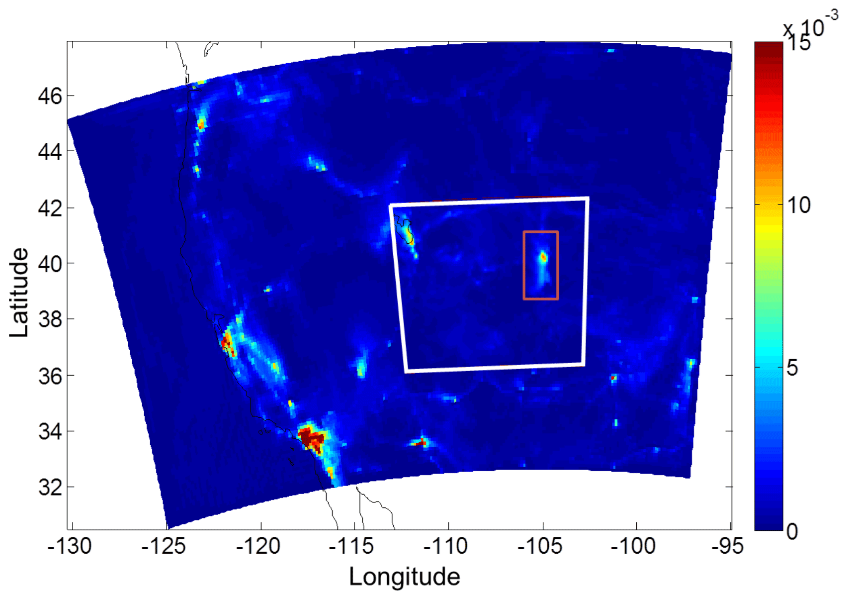
Figure 1Model domain is 12 km outer domain and 3 km inner domain. Data assimilation is performed on the inner domain.
The anthropogenic emissions are taken from the National Emission Inventory (NEI) 2011, which describes the hourly emissions for a typical summertime weekday. Biogenic emissions are parameterized using Model of Emissions of Gases and Aerosols from Nature (MEGAN) (Guenther et al., 2006). Gas-phase reactions are simulated using the regional acid deposition model version 2 (RADM2).
2.2 DART assimilation system
WRF-Chem-DART is a regional multivariate data assimilation system developed by the National Center for Atmospheric Research (NCAR) to analyze meteorological and chemical states simultaneously (Anderson and Collins 2007; Anderson et al., 2009). In this study we use the DART toolkit configured as the ensemble adjustment Kalman filter (EAKF) (Anderson, 2001). We apply adaptive spatially and temporally varying inflation to the prior state to maintain the ensemble spread (Anderson et al., 2009). We use horizontal localization to reduce the influence from spurious correlations (Anderson, 2012). A Gaspari and Cohn (1999) weighting function is applied with weights diminishing to zero 20 km away from the observation location. As in Liu et al. (2017), sensitivity tests show that NO2 data assimilation with an hour assimilation window performs the best using the weighting function with a width of 20 km. The analyzed chemical states are NO2 concentrations. The analyzed meteorological states include winds (U, V, W), temperature (T), cloud and cloud water properties (QVAPOR, QCLOUD, QRAIN, QICE, QSNOW), and other variables as described in Table 2 of Romine et al. (2013). The analysis is updated using DART from continuously cycled 1 h 30 member ensemble WRF-Chem forecasts. The DART configuration details are provided in Liu et al. (2017).
Previous studies that assimilate chemistry and meteorology simultaneously apply the variable localization approach (Arellano et al., 2007; Kang et al., 2011; Liu et al., 2017) which zeroes out the covariance between chemistry and some of the meteorology variables without taking advantage of the information related to meteorology carried by the chemical tracers. In this study, we partially turn off the variable localization and allow the assimilated NO2 observations to influence horizontal wind (U and V). With this setup, the advection scheme in the WRF-Chem model predicts downwind NO2 evolution based on the wind fields. The EAKF computes the covariances between the predicted NO2 distribution and wind variables. These sensitivities are utilized to refine the model state toward one that best fits the NO2 observations considering the confidence in both the observations and model prediction.
2.3 Initial and boundary condition ensembles
We add random perturbations to the temperature field of a single initial state to produce an ensemble of perturbed meteorological initial conditions. The perturbations were generated by sampling the Global Forecast System (GFS) background error covariance using the WRF data assimilation system (WRFDA) (Barker et al., 2012). (For those trying to repeat exactly, we used cv_option = 3.) The statistics are estimated with the differences of 24 and 48 h GFS forecasts with T170 (∼ 75 km) resolution, valid at the same time for 357 cases, distributed over a period of 1 year. The ensemble member lateral boundary condition perturbations are generated based on random variations within the initial ensemble (using the DART pert_wrf_bc program). Updating the boundary conditions so that the analysis time matches the analysis states from DART requires care in labeling (the DART update_wrf_bc program is used).
2.4 Synthetic observations
To generate synthetic TEMPO NO2 retrievals, we use the TEMPO NO2 simulator developed in Liu et al. (2017) as the observation operator to compute the observed column from a model prediction. It includes a layer-dependent box air mass factor (BAMF) for each observation pixel. BAMF is atmospheric scattering weights that depend on parameters including viewing geometry, surface (terrain or cloud) pressure and surface reflectivity. The parameters used to compute BAMFs are sampled from a model run with hourly frequency and clear sky conditions. Details for the TEMPO simulator and observation error generation are described in Liu et al. (2017). Note that we developed this simulator prior to the TEMPO science team creating its own product.
We perform observing system simulation experiments (OSSEs) to analyze the wind constraints from synthetic NO2 observations. We initialized the WRF-Chem nature run (NR) on a 12 km resolution domain (d01) on 1 June 2014 at 00:00 UTC. The meteorological initial and boundary conditions are taken from the NAM, and the chemistry simulation is constrained by MOZART output (see https://www.acom.ucar.edu/wrf-chem/mozart.shtml to download MOZART data, last access: 1 July 2020). After a 1-month simulation on d01, the NR on the 3 km domain (d02) is initialized from the d01 model simulation on 2 July 2014 at 15:00 UTC. Its meteorological and chemical boundary conditions are provided by NAM reanalysis data and the d01 simulation, respectively. We have a parallel model simulation labeled control run (CR) which is performed in the same way as the NR except its meteorological simulation is initialized and constrained by a different forecast model, the NARR. Constrained by different reanalysis data, the NR- and CR-simulated winds in the boundary layer differ and thus show the discrepancy in the NO2 transport processes. We perform data assimilation on d02 from 3 July 2014, 13:00 UTC, to 6 July 2014, 00:00 UTC, with an hourly assimilation window. This timing allows for analyses of three complete daytime cycles. In our OSSE, the NR simulations are considered as the “true atmosphere” from which synthetic NO2 observations are generated using the TEMPO simulator. After a 1 h forecast the prior ensemble is combined with synthetic NO2 observations to produce the posterior ensemble. The difference in wind and NO2 simulations between the NR and the ensemble mean results from the utilization of two different sets of reanalysis data as meteorological constraints and from the assimilation, while we apply the same forecast model, emission input, and model physics and chemistry scheme. The posterior ensemble will be used as the initial conditions to forecast the next hour. We evaluate the data assimilation performance by comparing the mean of the posterior estimate with the NR simulations.
We designed a series of six experiments to evaluate the potential of geostationary observations of column NO2 to improve wind fields. First, we conduct a free model run (FREE) with 30 ensemble members derived from the CR without data assimilation. This will set the baseline performance and will be compared with cases that assimilate observations to evaluate the benefit of data assimilation to improve the winds. In the second experiment (CHEM), we assimilate synthetic TEMPO NO2 observations over the 12 h daytime to constrain the winds in the ensemble. By comparing with FREE, we can evaluate the improvement in wind simulations as a result of assimilating NO2 observations. In experiment (T, RH), we assimilate hourly observations of temperature and humidity which can indirectly update winds via the covariances of temperature and humidity against wind states. In experiment (T, RH, CHEM), we assimilate synthetic TEMPO NO2 observations together with temperature and humidity observations. In this case, wind analyses are constrained by the multiple indirect observations via covariances with temperature, humidity and NO2. In the experiment (MET), we assimilate all meteorological observations including wind, temperature and humidity. This is representative of the current weather observing systems' representation of boundary layer winds. Finally, we assimilate synthetic TEMPO NO2 observations in addition to the meteorological observations in the experiment (MET, CHEM) to assess the influence of NO2 observations on winds under the circumstances of a full meteorology assimilation.
We compare the assimilation results with the NR states to evaluate the assimilation performance. The RMSE of the observed quantities are calculated as , where and are the model and true values for the ith observation, respectively, and n is the total number of observations located within a submodel space in Fig. 2. The RMSE of the model states are calculated as , where and are the model and true values at the ith model grid point, respectively, and l is the total number of grid points of interest. For the analyzed wind variables, the grid points of interest are all the points located within a model subdomain as shown in Fig. 2, containing the lowest five model levels vertically (∼ 250 m). We find that the horizontal transport of urban NO2 is most sensitive to the winds in the lowest five model levels, and the top of the shallow boundary layer in the morning is as low as the fifth model level. The likely scenario that power plant stacks result in emissions outside this vertical window was not explored in this study. We also analyze the uncertainty (spread) of the prior and posterior estimates. The uncertainty is calculated as the 1σ standard deviation of the ensemble.

Figure 2The U wind state variable at 07:00 UTC on 4 July (a) prior minus truth, (b) posterior minus truth, (c) posterior minus prior and (d) the difference between the prior TEMPO NO2 column and the truth.
4.1 NO2 assimilation
The performance of ensemble-based assimilation is determined by the representation of the ensemble uncertainty. In OSSEs we test how well the ensemble system represents the uncertainty by comparing the ensemble spread with the RMSE computed with respect to the true observations. Figure 3 shows the temporal evolution of the RMSE and the spread for synthetic TEMPO NO2 column observations in FREE and the three experiments with synthetic TEMPO observations assimilated. We find that in all experiments the variation in the prior ensemble spread follows the fluctuations of the prior RMSE with a similar magnitude after the first day of assimilation. This indicates that the ensemble system develops a good amount of spread for NO2 states and wind states as well because the NO2 spread results from the wind differences among ensemble members.
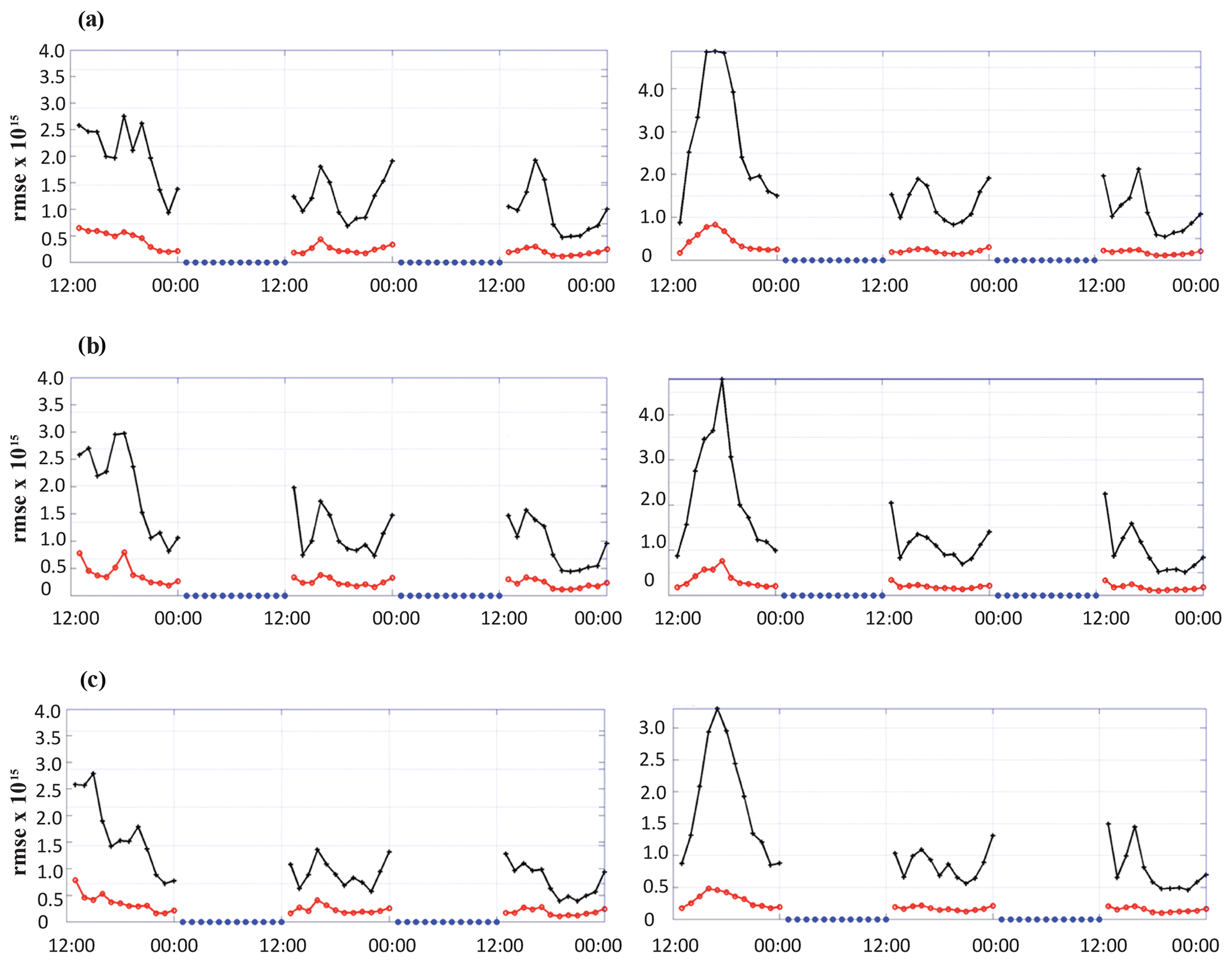
Figure 3(a) Evaluation of the time evolution of TEMPO column NO2 observations in Denver from 2 July at 16:00 to 5 July at 00:00 UTC for the CHEM experiment. Prior (black) and posterior (red). Left: RMSE, right: spread. (b) Evaluation of the pseudo TEMPO column NO2 observations in Denver from 2 July at 16:00 to 5 July at 00:00 UTC for the (T, RH, CHEM) experiment. Prior (black) and posterior (red). Left: RMSE, right: spread. (c) Evaluation of the time evolution of the pseudo TEMPO column NO2 observations in Denver from 2 July at 16:00 to 5 July at 00:00 UTC for the (MET, CHEM) experiment. Prior (black) and posterior (red). Left: RMSE, right: spread.
For all the experiments assimilating synthetic TEMPO NO2 observations, the diurnal variation in the prior RMSE and spread is related to the NO2 column variation with the peaks in the morning and evening rush hours and local minima in the early afternoon. The errors in the comparison to the synthetic TEMPO NO2 columns are reduced by 78 % on average from the prior to the posterior estimates. The temporal average of the posterior RMSE varies from 2.6 to 2.9 × 10¹⁴ molec. cm−2, which is very similar to the NO2 assimilation results in our previous experiment ENS.1 as shown in Fig. 4 of Liu et al. (2017). Experiment CHEM shows lower prior RMSE of TEMPO NO2 than the FREE for two reasons. First, assimilation of TEMPO in CHEM reduces the errors in the posterior NO2 of the last cycle, which results in better forecasts of prior NO2. Second, assimilation of NO2 improves the wind forecast in models (as shown in Sect. 4.2) and thus reduces the NO2 transport errors. This demonstrates that in places without wind observations, assimilating synthetic TEMPO NO2 observations can reduce the errors in the NO2 forecast by allowing NO2 observations to improve wind simulations in models.
4.2 Using synthetic TEMPO NO2 observations to constrain the winds
Errors of the winds in models affect the horizontal advection of NO2 and result in differences between observed and modeled NO2 vertical column density that can be used to correct the winds. In this ensemble assimilation system, we examine the impact of assimilating synthetic TEMPO NO2 observations on the winds in the boundary layer when different sets of meteorological observations are assimilated. Figure 4 shows the hourly evolution of the posterior RMSE of wind state variable U for all six experiments. Results for V are similar. We exclude the first daytime point in our analysis because it takes time for the assimilation system to equilibrate. Without any constraint on winds, FREE shows varying wind RMSE with higher values in the night than the daytime. With the assimilation of TEMPO only, CHEM shows error reduction in the posterior wind analysis in each daytime cycle (Fig. 4a). Table 1 compares the temporal average of the posterior wind RMSE for the six runs during daytime. The daytime average posterior RMSE is reduced by 0.44 m s−1 (15.70 %) and 0.41 m s−1 (15.45 %) for U and V wind from FREE to CHEM. We find that the reduction in wind RMSE resulting from daytime assimilation disappears after the first night cycle (Fig. 4). This is because the daytime error reduction is only observed in regions with abundant NO2 concentrations; wind errors in regions with little NO2 remain high during the day and quickly propagate into the regions with high daytime NO2 during the night once there is no longer any NO2 assimilation to constrain the error. As a result, the nighttime average RMSE of CHEM is very close to that of FREE, independent of the improvement of wind simulations from daytime. In the transition from night to daytime, the influence of assimilating NO2 observations on winds begins with the first daytime cycle. This demonstrates that the covariance of wind and NO2 develops and remains during the night.
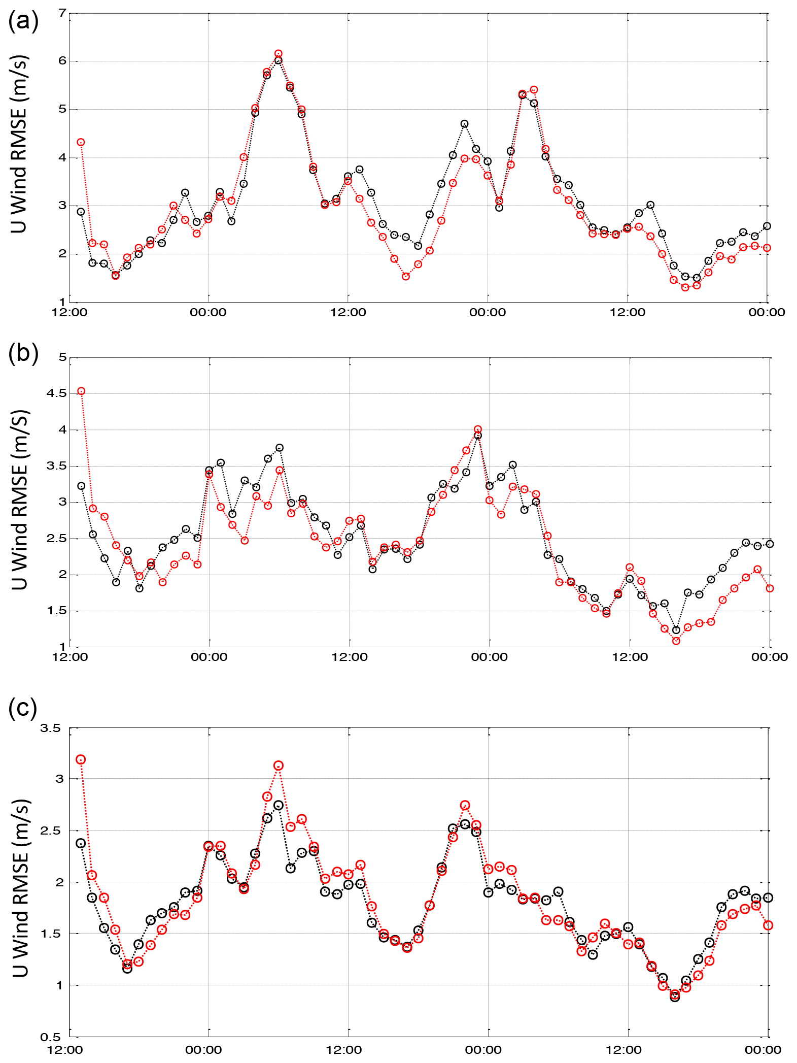
Figure 4RMSE for the U winds in the urban assimilation domain. (a) Free (black) vs. CHEM (red). (b) (T, RH) (black), (T, RH, CHEM) (red). (c) MET (black), (MET, CHEM) (red). Note the change in scale.
Figure 2a and b show the difference in U wind between the CHEM run and the truth at 13:00 MST on 4 July before and after assimilation. The incremental change in U wind after assimilation is plotted in Fig. 2c. The difference between the truth and the prior NO2 column amounts viewed by the TEMPO simulator is also shown in Fig. 2d. Because the U wind is underestimated in the prior, the modeled NO2 plume in the prior is more concentrated at the source and more dispersed to the east than in truth. After the assimilation of the synthetic TEMPO NO2 columns, we observe that the wind increases at the top and middle of the domain, where it was most underestimated prior to assimilation (Fig. 4). Averaged over the domain, the U wind RMSE is reduced from 2.32 to 1.56 m s−1 from the prior to the posterior.
Table 1RMSE of assimilated U (left) and V (right) daytime winds.
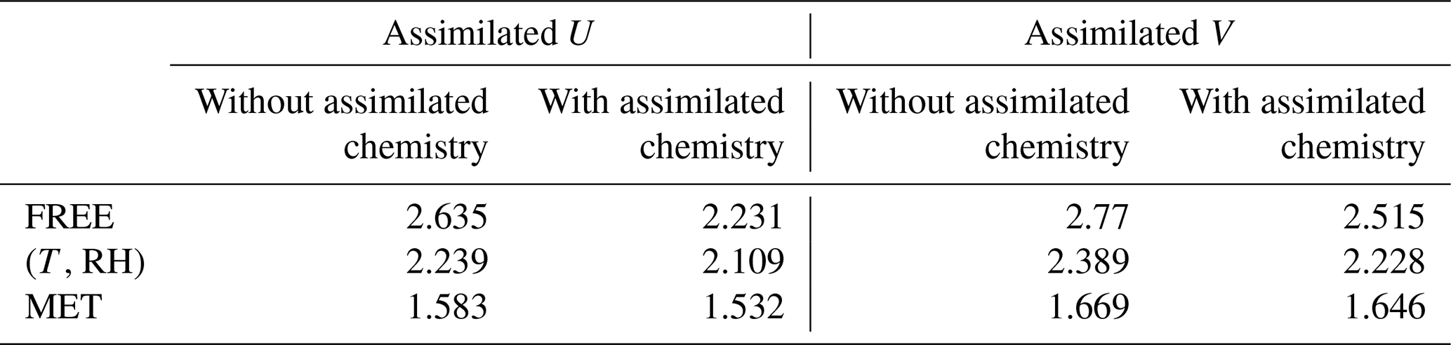
In the next two experiments (hereafter, T and RH, respectively) we assimilate observations of temperature and humidity in the (T, RH) run to adjust the wind variables. As shown in Table 1, (T, RH) shows 13.91 % and 15.10 % error reduction in posterior U and V winds during daytime compared to the unconstrained run FREE. These are improvements to winds from assimilating temperature and humidity observations using the covariances between meteorological variables. In addition, we find the averaged daytime posterior wind RMSE of (T, RH) is very close to that of the CHEM run. This demonstrates that TEMPO NO2 columns, as indirect chemical observations of winds, can be used to constrain winds, as well as temperature and humidity observations which are also indirect observations of winds. However, the temporal variations in the daytime posterior wind RMSE between the two runs are different (Fig. 4b). At the beginning of the daytime cycles, the (T, RH) run shows lower posterior wind RMSE than CHEM as temperature and humidity observations are assimilated during the night, resulting in lower nighttime wind errors, whereas no nighttime NO2 TEMPO observations are available to be assimilated. In the later daytime cycles, the posterior wind RMSE in CHEM becomes lower than that in (T, RH) due to the assimilations of TEMPO NO2.
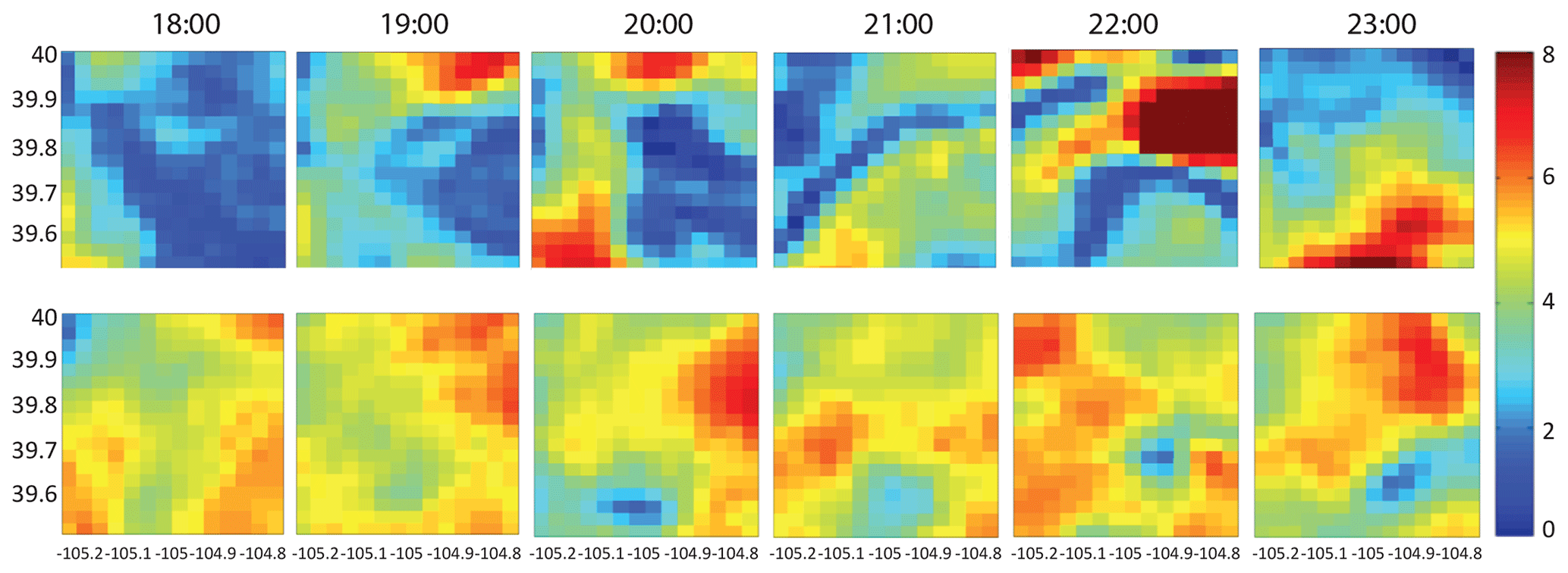
Figure 5Winds for successive hours from 18:00 to 23:00 UTC on the second (4 July – top row) and third (5 July – bottom row) days of the assimilation.
When we assimilate TEMPO NO2 together with temperature and humidity observations in (T, RH, CHEM), we find further error reductions in posterior wind during the third day compared with (T, RH) (Fig. 4b). This is because (T, RH) shows no error reductions in posterior winds in the afternoon of the third day, while the assimilation of TEMPO NO2 alone can successfully reduce wind errors (Fig. 4a). There are only minor differences between the (T, RH) and (T, RH, CHEM) runs during the second daytime. This is because assimilating temperature and humidity observations alone has reduced the wind errors to the extent that assimilations of additional NO2 observations can not provide further improvements. Furthermore, Fig. 5 shows the wind speed in the afternoon is mostly between 2 to 4 m s−1 on the second day (4 July) and 4–6 m s−1 on the third day (5 July). When the wind is stagnant, we do not expect strong covariances between winds and NO2 because the horizontal transport of NO2 due to wind is not strong. When wind speed is higher on the third day, it increases the ensemble covariances between wind and NO2 to achieve further improvement on wind.
The MET experiment has the lowest RMSE in the prior estimates of NO2 because it has the lowest wind errors, and thus NO2 transport errors, as a result of the assimilation of direct wind observations (Figs. 4c and 5). Nevertheless, even in this run there is a small benefit to assimilating NO2 columns as can be seen in the reduced RMSE of the wind on the third day.
The assimilation of column NO2 is explored as a constraint on boundary layer winds. Compared with assimilations of temperature and humidity, assimilations of column NO2 are as effective as a constraint on winds during the daytime. Column NO2 which is only available in sunlight is less effective than T and RH in the morning but more effective in the afternoon. In addition, we find that assimilating column NO2 as will be provided by the TEMPO satellite instrument does not degrade the results of assimilating temperature and humidity observations to constrain winds, and it improves on wind reanalysis, especially when wind speeds are above 4 m s−1. Including all available data, T, RH, winds and column NO2 makes it more difficult to discern the improvement from the NO2 column assimilation. Nevertheless, we observe improvements in wind reanalysis even under these circumstances (Table 1). This initial experiment covers a small domain surrounding the city of Denver and only a few days. With this initial study suggesting the method has promise, a larger-scale experiment should now be evaluated. We hope this study will inspire such research.
The data used in this paper and the associated software packages are available via the Github open repository via the following links, with descriptions (last access: 20 June 2020); https://github.com/NCAR/DART (Anderson and Collins, 2007; the ensemble Kalman filter solver and the WRF-Chem/DART interface code), https://github.com/NCAR?q=wrf&type=&language=&sort= (Skamarock et al., 2008; WRF model, as well as access to utilities used by WRF-Chem-DART, and ensemble spread for meteorology), and https://github.com/NCAR/WPS (Skamarock et al., 2008; the WRF pre-processor for taking large scale meteorology fields and putting them into WRF input format).
Data for this analysis have not been archived as their size is too large, but they can be recreated with the software described above.
XL and RCC conceived the project, and XL developed and executed the numerical experiments. APM, JLA, IF and RCC contributed to the design of the experiments and interpretation of the results. XL and RCC prepared the manuscript with contributions from all co-authors.
The authors declare that they have no conflict of interest.
We thank Nancy Collins (NCAR/IMAGe) and Tim Hoar (NCAR/IMAGe) for the assistance with DART. We would like to acknowledge high-performance computing support from Yellowstone (ark:/85065/d7wd3xhc) provided by NCAR's Computational and Information Systems Laboratory, sponsored by the National Science Foundation.
This research has been supported by NASA (grant nos. NNX10AR36G and NNX15AE37G) and the Smithsonian Astrophysical Observatory (grant no. SV3-83019).
This paper was edited by Abhishek Chatterjee and reviewed by three anonymous referees.
Allen, D. R., Hoppel, K. W., Nedoluha, G. E., Kuhl, D. D., Baker, N. L., Xu, L., and Rosmond, T. E.: Limitations of wind extraction from 4D-Var assimilation of ozone, Atmos. Chem. Phys., 13, 3501–3515, https://doi.org/10.5194/acp-13-3501-2013, 2013.
Allen, D. R., Hoppel, K. W., and Kuhl, D. D.: Wind extraction potential from 4D-Var assimilation of stratospheric O3, N2O, and H2O using a global shallow water model, Atmos. Chem. Phys., 14, 3347–3360, https://doi.org/10.5194/acp-14-3347-2014, 2014.
Allen, D. R., Hoppel, K. W., and Kuhl, D. D.: Wind extraction potential from ensemble Kalman filter assimilation of stratospheric ozone using a global shallow water model, Atmos. Chem. Phys., 15, 5835–5850, https://doi.org/10.5194/acp-15-5835-2015, 2015.
Anderson, J. and Collins, N.: Scalable Implementations of Ensemble Filter Algorithms for Data Assimilation, J. Atmos. Ocean. Technol., 24, 1452–1463, https://doi.org/10.1175/JTECH2049.1, 2007 (code available at: https://github.com/NCAR/DART, last access: 20 June 2020).
Anderson, J., Hoar, T., Raeder, K., Liu, H., Collins, N., Torn, R., and Avellano, A.: The Data Assimilation Research Testbed: A Community Facility, Bull. Am. Meteorol. Soc., 90, 1283–1296, https://doi.org/10.1175/2009BAMS2618.1, 2009.
Anderson, J. L.: An Ensemble Adjustment Kalman Filter for Data Assimilation, Mon. Weather Rev., 129, 2884–2903, https://doi.org/10.1175/1520-0493(2001)129<2884:AEAKFF>2.0.CO;2, 2001.
Anderson, J. L.: Localization and Sampling Error Correction in Ensemble Kalman Filter Data Assimilation, Mon. Weather Rev., 140, 2359–2371, https://doi.org/10.1175/MWR-D-11-00013.1, 2012.
Arellano Jr., A. F., Raeder, K., Anderson, J. L., Hess, P. G., Emmons, L. K., Edwards, D. P., Pfister, G. G., Campos, T. L., and Sachse, G. W.: Evaluating model performance of an ensemble-based chemical data assimilation system during INTEX-B field mission, Atmos. Chem. Phys., 7, 5695–5710, https://doi.org/10.5194/acp-7-5695-2007, 2007.
Baklanov, A., Schlünzen, K., Suppan, P., Baldasano, J., Brunner, D., Aksoyoglu, S., Carmichael, G., Douros, J., Flemming, J., Forkel, R., Galmarini, S., Gauss, M., Grell, G., Hirtl, M., Joffre, S., Jorba, O., Kaas, E., Kaasik, M., Kallos, G., Kong, X., Korsholm, U., Kurganskiy, A., Kushta, J., Lohmann, U., Mahura, A., Manders-Groot, A., Maurizi, A., Moussiopoulos, N., Rao, S. T., Savage, N., Seigneur, C., Sokhi, R. S., Solazzo, E., Solomos, S., Sørensen, B., Tsegas, G., Vignati, E., Vogel, B., and Zhang, Y.: Online coupled regional meteorology chemistry models in Europe: current status and prospects, Atmos. Chem. Phys., 14, 317–398, https://doi.org/10.5194/acp-14-317-2014, 2014.
Barker, D., Huang, X.-Y., Liu, Z., Auligné, T., Zhang, X., Rugg, S., Ajjaji, R., Bourgeois, A., Bray, J., Chen, Y., Demirtas, M., Guo, Y.-R., Henderson, T., Huang, W., Lin, H.-C., Michalakes, J., Rizvi, S., and Zhang, X.: The Weather Research and Forecasting Model's Community Variational/Ensemble Data Assimilation System: WRFDA, Bull. Am. Meteorol. Soc., 93, 831–843, https://doi.org/10.1175/BAMS-D-11-00167.1, 2012.
Bauer, P., Thorpe, A., and Brunet, G.: The quiet revolution of numerical weather prediction, Nature, 525, 47–55, https://doi.org/10.1038/nature14956, 2015.
Beirle, S., Boersma, K. F., Platt, U., Lawrence, M. G., and Wagner, T.: Megacity emissions and lifetimes of nitrogen oxides probed from space, Science, 333, 1737–9, https://doi.org/10.1126/science.1207824, 2011.
Bocquet, M., Elbern, H., Eskes, H., Hirtl, M., Žabkar, R., Carmichael, G. R., Flemming, J., Inness, A., Pagowski, M., Pérez Camaño, J. L., Saide, P. E., San Jose, R., Sofiev, M., Vira, J., Baklanov, A., Carnevale, C., Grell, G., and Seigneur, C.: Data assimilation in atmospheric chemistry models: current status and future prospects for coupled chemistry meteorology models, Atmos. Chem. Phys., 15, 5325–5358, https://doi.org/10.5194/acp-15-5325-2015, 2015.
Chu, D. A., Tsai, T.-C., Chen, J.-P., Chang, S.-C., Jeng, Y.-J., Chiang, W.-L., and Lin, N.-H.: Interpreting aerosol lidar profiles to better estimate surface PM2.5 for columnar AOD measurements, Atmos. Environ., 79, 172–187, https://doi.org/10.1016/j.atmosenv.2013.06.031, 2013.
Dee, D. P., Balmaseda, M., Balsamo, G., Engelen, R., Simmons, A. J., and Thépaut, J.-N.: Toward a Consistent Reanalysis of the Climate System, Bull. Amer. Meteor. Soc., 95, 1235–1248, https://doi.org/10.1175/BAMS-D-13-00043.1, 2014.
Emili, E., Gürol, S., and Cariolle, D.: Accounting for model error in air quality forecasts: an application of 4DEnVar to the assimilation of atmospheric composition using QG-Chem 1.0, Geosci. Model Dev., 9, 3933–3959, https://doi.org/10.5194/gmd-9-3933-2016, 2016.
Emmons, L. K., Walters, S., Hess, P. G., Lamarque, J.-F., Pfister, G. G., Fillmore, D., Granier, C., Guenther, A., Kinnison, D., Laepple, T., Orlando, J., Tie, X., Tyndall, G., Wiedinmyer, C., Baughcum, S. L., and Kloster, S.: Description and evaluation of the Model for Ozone and Related chemical Tracers, version 4 (MOZART-4), Geosci. Model Dev., 3, 43–67, https://doi.org/10.5194/gmd-3-43-2010, 2010.
Fiore, A. M., Naik, V., Spracklen, D. V, Steiner, A., Unger, N., Prather, M., Bergmann, D., Cameron-Smith, P. J., Cionni, I., Collins, W. J., Dalsøren, S., Eyring, V., Folberth, G. A., Ginoux, P., Horowitz, L. W., Josse, B., Lamarque, J.-F., MacKenzie, I. A., Nagashima, T., O'Connor, F. M., Righi, M., Rumbold, S. T., Shindell, D. T., Skeie, R. B., Sudo, K., Szopa, S., Takemura, T., and Zeng, G.: Global air quality and climate, Chem. Soc. Rev., 41, 6663–6683, https://doi.org/10.1039/c2cs35095e, 2012.
Flemming, J., Huijnen, V., Arteta, J., Bechtold, P., Beljaars, A., Blechschmidt, A.-M., Diamantakis, M., Engelen, R. J., Gaudel, A., Inness, A., Jones, L., Josse, B., Katragkou, E., Marecal, V., Peuch, V.-H., Richter, A., Schultz, M. G., Stein, O., and Tsikerdekis, A.: Tropospheric chemistry in the Integrated Forecasting System of ECMWF, Geosci. Model Dev., 8, 975–1003, https://doi.org/10.5194/gmd-8-975-2015, 2015.
Gaspari, G. and Cohn, S. E.: Construction of correlation functions in two and three dimensions, Q. J. R. Meteorol. Soc., 125, 723–757, https://doi.org/10.1002/qj.49712555417, 1999.
Gelaro, R., McCarty, W., Suárez, M. J., Todling, R., Molod, A., Takacs, L., Randles, C. A., Darmenov, A., Bosilovich, M. G., Reichle, R., Wargan, K., Coy, L., Cullather, R., Draper, C., Akella, S., Buchard, V., Conaty, A., da Silva, A. M., Gu, W., Kim, G. K., Koster, R., Lucchesi, R., Merkova, D., Nielsen, J. E., Partyka, G., Pawson, S., Putman, W., Rienecker, M., Schubert, S. D., Sienkiewicz, M., and Zhao, B.: The modern-era retrospective analysis for research and applications, version 2 (MERRA-2), J. Climate, 30, 5419–5454, https://doi.org/10.1175/JCLI-D-16-0758.1, 2017.
Grell, G. and Baklanov, A.: Integrated modeling for forecasting weather and air quality: A call for fully coupled approaches, Atmos. Environ., 45, 6845–6851, https://doi.org/10.1016/j.atmosenv.2011.01.017, 2011.
Grell, G., Freitas, S. R., Stuefer, M., and Fast, J.: Inclusion of biomass burning in WRF-Chem: impact of wildfires on weather forecasts, Atmos. Chem. Phys., 11, 5289–5303, https://doi.org/10.5194/acp-11-5289-2011, 2011.
Guenther, A., Karl, T., Harley, P., Wiedinmyer, C., Palmer, P. I., and Geron, C.: Estimates of global terrestrial isoprene emissions using MEGAN (Model of Emissions of Gases and Aerosols from Nature), Atmos. Chem. Phys., 6, 3181–3210, https://doi.org/10.5194/acp-6-3181-2006, 2006.
Haussaire, J.-M. and Bocquet, M.: A low-order coupled chemistry meteorology model for testing online and offline data assimilation schemes: L95-GRS (v1.0), Geosci. Model Dev., 9, 393–412, https://doi.org/10.5194/gmd-9-393-2016, 2016.
Inness, A., Baier, F., Benedetti, A., Bouarar, I., Chabrillat, S., Clark, H., Clerbaux, C., Coheur, P., Engelen, R. J., Errera, Q., Flemming, J., George, M., Granier, C., Hadji-Lazaro, J., Huijnen, V., Hurtmans, D., Jones, L., Kaiser, J. W., Kapsomenakis, J., Lefever, K., Leitão, J., Razinger, M., Richter, A., Schultz, M. G., Simmons, A. J., Suttie, M., Stein, O., Thépaut, J.-N., Thouret, V., Vrekoussis, M., Zerefos, C., and the MACC team: The MACC reanalysis: an 8 yr data set of atmospheric composition, Atmos. Chem. Phys., 13, 4073–4109, https://doi.org/10.5194/acp-13-4073-2013, 2013.
Inness, A., Blechschmidt, A.-M., Bouarar, I., Chabrillat, S., Crepulja, M., Engelen, R. J., Eskes, H., Flemming, J., Gaudel, A., Hendrick, F., Huijnen, V., Jones, L., Kapsomenakis, J., Katragkou, E., Keppens, A., Langerock, B., de Mazière, M., Melas, D., Parrington, M., Peuch, V. H., Razinger, M., Richter, A., Schultz, M. G., Suttie, M., Thouret, V., Vrekoussis, M., Wagner, A., and Zerefos, C.: Data assimilation of satellite-retrieved ozone, carbon monoxide and nitrogen dioxide with ECMWF's Composition-IFS, Atmos. Chem. Phys., 15, 5275–5303, https://doi.org/10.5194/acp-15-5275-2015, 2015.
Inness, A., Flemming, J., Heue, K.-P., Lerot, C., Loyola, D., Ribas, R., Valks, P., van Roozendael, M., Xu, J., and Zimmer, W.: Monitoring and assimilation tests with TROPOMI data in the CAMS system: near-real-time total column ozone, Atmos. Chem. Phys., 19, 3939–3962, https://doi.org/10.5194/acp-19-3939-2019, 2019.
Kang, J.-S., E. Kalnay, J. Liu, I. Fung, T. Miyoshi, and K. Ide: Variable localization in an ensemble Kalman filter: Application to the carbon cycle data assimilation, J. Geophys. Res., 116, D09110, https://doi.org/10.1029/2010JD014673, 2011.
Lahoz, W. A., Errera, Q., Swinbank, R., and Fonteyn, D.: Data assimilation of stratospheric constituents: a review, Atmos. Chem. Phys., 7, 5745–5773, https://doi.org/10.5194/acp-7-5745-2007, 2007.
Laughner, J. L. and Cohen, R. C.: Direct observation of changing NOx lifetime in North American cities, Science, 366, 723–727, https://doi.org/10.1126/science.aax6832, 2019.
Laughner, J. L., Zare, A., and Cohen, R. C.: Effects of daily meteorology on the interpretation of space-based remote sensing of NO2, Atmos. Chem. Phys., 16, 15247–15264, https://doi.org/10.5194/acp-16-15247-2016, 2016.
Lin, J.-T.: Satellite constraint for emissions of nitrogen oxides from anthropogenic, lightning and soil sources over East China on a high-resolution grid, Atmos. Chem. Phys., 12, 2881–2898, https://doi.org/10.5194/acp-12-2881-2012, 2012.
Liu, J., Fung, I., Kalnay, E., Kang, J.-S., Olsen, E. T., and Chen, L.: Simultaneous assimilation of AIRS XCO2 and meteorological observations in a carbon climate model with an ensemble Kalman filter, J. Geophys. Res., 117, D05309, https://doi.org/10.1029/2011JD016642, 2012.
Liu, X., Mizzi, A. P., Anderson, J. L., Fung, I. Y., and Cohen, R. C.: Assimilation of satellite NO2 observations at high spatial resolution using OSSEs, Atmos. Chem. Phys., 17, 7067–7081, https://doi.org/10.5194/acp-17-7067-2017, 2017.
Mebust, A. K., Russell, A. R., Hudman, R. C., Valin, L. C., and Cohen, R. C.: Characterization of wildfire NOx emissions using MODIS fire radiative power and OMI tropospheric NO2 columns, Atmos. Chem. Phys., 11, 5839–5851, https://doi.org/10.5194/acp-11-5839-2011, 2011.
Ménard, R., Gauthier, P., Rochon, Y., Robichaud, A., de Grandpré, J., Yang, Y., Charrette, C., and Chabrillat, S.: Coupled Stratospheric Chemistry–Meteorology Data Assimilation. Part II: Weak and Strong Coupling, Atmosphere, 10, 798, https://doi.org/10.3390/atmos10120798, 2019.
Milewski, T. and Bourqui, M. S.: Assimilation of Stratospheric Temperature and Ozone with an Ensemble Kalman Filter in a Chemistry–Climate Model, Mon. Weather Rev., 139, 3389–3404, https://doi.org/10.1175/2011MWR3540.1, 2011.
Miyazaki, K., Eskes, H. J., Sudo, K., and Zhang, C.: Global lightning NOx production estimated by an assimilation of multiple satellite data sets, Atmos. Chem. Phys., 14, 3277–3305, https://doi.org/10.5194/acp-14-3277-2014, 2014.
Miyazaki, K., Eskes, H., Sudo, K., Boersma, K. F., Bowman, K., and Kanaya, Y.: Decadal changes in global surface NOx emissions from multi-constituent satellite data assimilation, Atmos. Chem. Phys., 17, 807–837, https://doi.org/10.5194/acp-17-807-2017, 2017.
Miyazaki, K., Bowman, K. W., Yumimoto, K., Walker, T., and Sudo, K.: Evaluation of a multi-model, multi-constituent assimilation framework for tropospheric chemical reanalysis, Atmos. Chem. Phys., 20, 931–967, https://doi.org/10.5194/acp-20-931-2020, 2020.
Mizzi, A. P., Arellano Jr., A. F., Edwards, D. P., Anderson, J. L., and Pfister, G. G.: Assimilating compact phase space retrievals of atmospheric composition with WRF-Chem/DART: a regional chemical transport/ensemble Kalman filter data assimilation system, Geosci. Model Dev., 9, 965–978, https://doi.org/10.5194/gmd-9-965-2016, 2016.
Peuch, A., Thépaut, J.-N., and Pailleux, J.: Dynamical impact of total-ozone observations in a four-dimensional variational assimilation, Q. J. Roy. Meteor. Soc., 126, 1641–1659, https://doi.org/10.1002/qj.49712656605, 2000.
Reale, O., Lau, K. M., and da Silva, A.: Impact of Interactive Aerosol on the African Easterly Jet in the NASA GEOS-5 Global Forecasting System, Weather Forecast., 26, 504–519, https://doi.org/10.1175/WAF-D-10-05025.1, 2011.
Reale, O., Lau, K. M., da Silva, A., and Matsui, T.: Impact of assimilated and interactive aerosol on tropical cyclogenesis, Geophys. Res. Lett., 41, 3282–3288, https://doi.org/10.1002/2014GL059918, 2014.
Romine, G. S., Schwartz, C. S., Snyder, C., Anderson, J. L., and Weisman, M. L.: Model bias in a continuously cycled assimilation system and its influence on convection-permitting forecasts, Mon. Weather Rev., 141, 1263–1284, https://doi.org/10.1175/MWR-D-12-00112.1, 2013.
Russell, A. R., Valin, L. C., and Cohen, R. C.: Trends in OMI NO2 observations over the United States: effects of emission control technology and the economic recession, Atmos. Chem. Phys., 12, 12197–12209, https://doi.org/10.5194/acp-12-12197-2012, 2012.
Saide, P. E., Carmichael, G. R., Spak, S. N., Minnis, P., and Ayers, J. K.: Improving aerosol distributions below clouds by assimilating satellite-retrieved cloud droplet number, Proc. Natl. Acad. Sci., USA, 109, 11939–11943, https://doi.org/10.1073/pnas.1205877109, 2012.
Saide, P. E., Kim, J., Song, C. H., Choi, M., Cheng, Y., and Carmichael, G. R.: Assimilation of next generation geostationary aerosol optical depth retrievals to improve air quality simulations, Geophys. Res. Lett., 41, 9188–9196, https://doi.org/10.1002/2014GL062089, 2014.
Semane, N., Peuch, V.-H., Pradier, S., Desroziers, G., El Amraoui, L., Brousseau, P., Massart, S., Chapnik, B., and Peuch, A.: On the extraction of wind information from the assimilation of ozone profiles in Météo–France 4-D-Var operational NWP suite, Atmos. Chem. Phys., 9, 4855–4867, https://doi.org/10.5194/acp-9-4855-2009, 2009.
Skamarock, W. C., Klemp, J. B., Dudhia, J., Gill, D. O., Barker, D., Duda, M. G., Huang, X., Wang, W., and Powers, J. G.: A Description of the Advanced Research WRF Version 3 (No. NCAR/TN-475+STR), University Corporation for Atmospheric Research, https://doi.org/10.5065/D68S4MVH, 2008 (codes available at: https://github.com/NCAR?q=wrf&type=&language=&sort= and https://github.com/NCAR/WPS, last access: 20 June 2020).
Tondeur, M., Carrassi, A., and Vannitsem, S.: On Temporal Scale Separation in Coupled Data Assimilation with the Ensemble Kalman Filter, J. Stat. Phys., 179, 1161–1185, https://doi.org/10.1007/s10955-020-02525-z, 2020.
Valin, L. C., Russell, A. R., and Cohen, R. C.: Variations of OH radical in an urban plume inferred from NO2 column measurements, Geophys. Res. Lett., 40, 1856–1860, 2013.
Xian, P., Reid, J. S., Hyer, E. J., Sampson, C. R., Rubin, J. I., Ades, M., Asencio, N., Basart, S., Benedetti, A., Bhattacharjee, P. S., Brooks, M. E., Colarco, P. R., da Silva, A. M., Eck, T. F., Guth, J., Jorba, O., Kouznetsov, R., Kipling, Z., Sofiev, M., Garcia-Pando, C. P., Pradhan, Y., Tanaka, T., Wang, J., Westphal, D. L., Yumimoto, K., and Zhan, J.: Current state of the global operational aerosol multi-model ensemble: An update from the International Cooperative for Aerosol Prediction (ICAP), Q. J. R. Meteorol. Soc., 145, 176–209, https://doi.org/10.1002/qj.3497, 2019.
Zhang, Y., Bocquet, M., Mallet, V., Seigneur, C., and Baklanov, A.: Real-time air quality forecasting, part II: State of the science, current research needs, and future prospects, Atmos. Environ., 60, 656–676, https://doi.org/10.1016/j.atmosenv.2012.02.041, 2012.
Zhu, Q., Laughner, J. L., and Cohen, R. C.: Lightning NO2 simulation over the contiguous US and its effects on satellite NO2 retrievals, Atmos. Chem. Phys., 19, 13067–13078, https://doi.org/10.5194/acp-19-13067-2019, 2019.
Zoogman, P., Liu, X., Suleiman, R. M., Pennington, W. F., Flittner, D. E., Al-Saadi, J. A., Hilton, B. B., Nicks, D. K., Newchurch, M. J., Carr, J. L., Janz, S. J., Andraschko, M. R., Baker, B. B., Canova, B. P., Chan Miller, C., Cohen, R. C., Davis, J. E., Dussault, M. E., Edwards, D. P., Fishman, J., González Abad, G., Grutter de la Mora, M., Herman, J. R., Houck, J., Jacob, D. J., Joiner, J., Kerridge, B. J., Kim, J., Krotkov, N. A., Martin, R. V., McElroy, C. T., McLinden, C., Natraj, V., Neil, D. O., Nowlan, C. R., O'Sullivan, E. J., Palmer, P. I., Pippin, M. R., Saiz-Lopez, A., Spurr, R. J. D., Szykman, J. J., Torres, O. O., Veefkind, J. P., Veihelmann, B., Wang, H., Wang, J., Wulamu, A., and Chance, K.: Tropospheric Emissions: Monitoring of Pollution (TEMPO), J. Quant. Spec. Rad. Trans., 186, 17–39, 2017.