the Creative Commons Attribution 4.0 License.
the Creative Commons Attribution 4.0 License.
 | 17 Jun 2021
Non-linear response of PM2.5 to changes in NOx and NH3 emissions in the Po basin (Italy): consequences for air quality plans
Philippe Thunis
Alain Clappier
Matthias Beekmann
Jean Philippe Putaud
Cornelis Cuvelier
Jessie Madrazo
Alexander de Meij
Air pollution is one of the main causes of damages to human health in Europe, with an estimate of about 380 000 premature deaths per year in the EU28, as the result of exposure to fine particulate matter (PM2.5) only. In this work, we focus on one specific region in Europe, the Po basin, a region where chemical regimes are the most complex, showing important non-linear processes, especially those related to interactions between NOx and NH3. We analyse the sensitivity of PM2.5 concentration to NOx and NH3 emissions by means of a set of EMEP model simulations performed with different levels of emission reductions, from 25 % up to a total switch-off of those emissions. Both single and combined precursor reduction scenarios are applied to determine the most efficient emission reduction strategies and quantify the interactions between NOx and NH3 emission reductions. The results confirmed the peculiarity of secondary PM2.5 formation in the Po basin, characterised by contrasting chemical regimes within distances of a few (hundred) kilometres, as well as non-linear responses to emission reductions during wintertime. One of the striking results is the slight increase in the PM2.5 concentration levels when NOx emission reductions are applied in NOx-rich areas, such as the surroundings of Bergamo. The increased oxidative capacity of the atmosphere is the cause of the increase in PM2.5 induced by a reduction in NOx emission. This process could have contributed to the absence of a significant PM2.5 concentration decrease during the COVID-19 lockdowns in many European cities. It is important to account for this process when designing air quality plans, since it could well lead to transitionary increases in PM2.5 at some locations in winter as NOx emission reduction measures are gradually implemented. While PM2.5 chemical regimes, determined by the relative importance of the NOx vs. NH3 responses to emission reductions, show large variations seasonally and spatially, they are not very sensitive to moderate (up to 50 %–60 %) emission reductions. Beyond 25 % emission reduction strength, responses of PM2.5 concentrations to NOx emission reductions become non-linear in certain areas of the Po basin mainly during wintertime.
- Article
(18000 KB) - Full-text XML
- BibTeX
- EndNote


Air pollution is one of the main causes of damages to human health in Europe, with an estimate of about 380 000 premature deaths per year in the EU28, as the result of exposure to fine particulate matter (PM2.5) only (EEA, 2020). Many of the exceedances to the EU limit values occur in urban areas where most of the population is exposed.
PM2.5 is partly emitted directly (primary particles) and partly formed through photo-chemical reactions that involve gaseous precursors like SOx, NOx, NH3 and non-methane volatile organic compounds (NMVOC) to form secondary inorganic and organic aerosol (SIA and SOA). The secondary fraction is often dominating the total concentration of particulate matter in urban areas as shown by e.g. Beekmann et al. (2015) for the Greater Paris region and by De Meij et al. (2006, 2009) or Larsen et al. (2012) in northern Italy, hence the importance of understanding the complex chemical processes that lead to its formation. In particular, it is key to identify the precursors involved in these reactions in order to target the right sectors of activity in air quality plans to effectively reduce pollution levels. According to the EDGAR estimates for 2015 for Italy, about 90 % of the NH3 is directly emitted in the atmosphere by the agriculture sector, while SOx precursors are predominantly released by the energy production and use (industrial) sectors (EDGAR, 2020). For NOx, emissions are spread among various sectors, with transport (50 %), industry (40 %) and agriculture (4 %) being the main ones. The gaseous precursors of secondary organic aerosols (SOA) include a vast range of NMVOCs among which are biogenic terpenes and anthropogenic aromatics. The main sources of aromatics in Italy were in 2012 transport (58 %), use of fuels and solvents (32 %), and domestic heating (15 %) (EDGAR, 2020).
Regarding SIA, early works used box models with thermodynamic schemes to address the sensitivity of ammonium nitrate and sulfate concentrations to gaseous NH3, NOx and SO2 emissions (Watson et al., 1994; Blanchard and Hidy, 2003; Pozzer et al., 2017; Guo et al., 2018; Nenes et al., 2020). These models were later on integrated into chemical transport models (CTMs), in particular to address the benefit of additional NH3 emission reductions in addition to already ongoing SO2 and NOx emission reductions. For North America, Makar et al. (2009) simulated with a regional CTM that a 30 % reduction of ammonia emissions would lead to about 1 µg m−3 reduction in PM2.5. For Europe, Bessagnet et al. (2014) simulated the effects of a 30 % NH3 emission reduction in addition to those foreseen by the Gothenburg Protocol for 2030 and found that the G ratio defined as the ratio between free ammonia and total nitrate (Ansari and Pandis, 1998) was a good predictor for the efficiency of NH3 reductions on SIA concentrations. These sensitivities to emission reductions are often governed by complex chemical mechanisms. A well-known phenomenon is the release of free ammonia as a result of decreased SO2 emissions and sulfate formation, which allows for the formation of additional particulate nitrate, as described for example by Blanchard and Hidy (2003) and Shah et al. (2018) for wintertime PM2.5 over the eastern United States. For eastern China, Fu et al. (2017) and Lachatre et al. (2019) showed both from modelling and satellite observations that such processes lead to strongly increased ammonia tropospheric columns. Finally, several works compared CTM simulations to specific observations. For instance, Pay et al. (2012) showed that the G ratio was generally underestimated over Europe, inducing that the Caliope model they used could probably overestimate the efficiency of NH3 emission reductions. Petetin et al. (2016) came to a similar conclusion comparing CHIMERE CTM simulations to observations in the Paris region. They ascribed this underestimation to missing NH3 emissions especially during warmer periods.
The formation of SOA results from even more complex reactions involving photo-chemical oxidation (as for SIA), nitration, fragmentation and oligomerisation of gaseous precursors or secondary products (Kroll and Seinfeld, 2008; Shrivastava et al., 2017). Models generally use simplified parameterisations to calculate the SOA formation yield from various classes of parent VOCs (Tsigaridis et al., 2014), and comparison with measurements often shows that SOA sources are still missing in models (Huang et al., 2020; Tsimpidi, 2016).
In this work, we focus on one specific region in Europe, the Po basin. In a companion paper (Clappier et al., 2021) that analyses PM secondary formation chemical regimes across Europe, the Po basin is clearly identified as a peculiar area where the chemical regime distributions are the most complex, showing non-linear processes (Thunis et al., 2013, 2015; Carnevale, 2020; Bessagnet, 2014), especially those related to interactions between NOx and NH3. The Po basin is also one of the pollution hot spots in Europe where the number of days above the limit values prescribed by the European Ambient Air Quality Directives (AAQD) for PM10 is yet largely exceeded (EEA, 2020). This situation results from the high emission density in this region and also from the geographical setting of the area, in the border of the Alps and Apennines mountain ranges that lead to very weak winds in the area, favouring the accumulation of atmospheric pollutants.
We focus the present analysis on the NH3–NOx chemical processes and describe their spatial and seasonal variability, which could help to design more effective mitigation strategies. We start by describing the modelling set-up and detail the series of simulations required to perform our analysis. Section 3 provides a brief overview of the modelled base-case concentrations. In Sect. 4, we analyse the sensitivity of PM2.5 concentrations to NH3 and NOx emissions. Section 5 provides an analysis of the non-linearity in PM2.5 response to these emissions, while in Sect. 6 we discuss the implications of these results in terms of mitigation measures and design of air quality plans. Conclusions are finally proposed.
2.1 Modelling set-up
The modelling study is performed with the EMEP air quality model, version rv4_17 (Simpson et al., 2012). The emission input consists of gridded annual national emissions (SO2, NO, NO2, NH3, NMVOC, CO and primary PM2.5) at 0.1×0.1∘ resolution, based on data reported every year by parties to the Convention on Long-range Transboundary Air Pollution (CLRTAP). These emissions are provided for 10 anthropogenic source sectors classified by SNAP (Selected Nomenclature for Air Pollution) codes (EMEP, 2003). Meteorological input data are based on forecasts from the Integrated Forecasting System (IFS), a global operational forecasting model from the European Centre for Medium-Range Weather Forecasts (ECMWF). Meteorological fields are retrieved at a 0.1×0.1∘ longitude–latitude resolution and are interpolated to the 50×50 km2 polar stereographic grid projection (EMEP, 2011).
The gas-phase chemistry is based on the evolution of the so-called “EMEP scheme” as described in Simpson et al. (2012) and references therein. The chemical scheme couples the sulfur and nitrogen chemistry to the photochemistry using about 140 reactions between 70 species (Andersson-Sköld and Simpson, 1999; Simpson et al., 2012). In the EMEP Status Report 1/2004 (Fagerli et al., 2004) the reactions that cover acidification, eutrophication and ammonium chemistry are described. The aqueous-phase chemistry describes the formation of sulfate in clouds via SO2 oxidation by ozone and H2O2 and catalysed by metal ions. An important pathway of particulate nitrate formation is through the hydrolysis of N2O5 on wet aerosol surfaces that converts NOx into HNO3. More information on the chemical equations is given in Simpson et al. (2012), Sect. 7.
The EMEP model has two size fractions for aerosols, fine aerosol (PM2.5) and coarse aerosol (PM10−2.5). The aerosol components presently accounted for are sulfate (SO), nitrate (NO), ammonium (NH), anthropogenic primary PM and sea salt.
For inorganic aerosols, EMEP uses the MARS equilibrium module to calculate the partitioning between gas and fine-mode aerosol phase in the system of SO, HNO3, NO, NH3 and NH (Binkowski and Shankar, 1995). Aerosol water is calculated to account for particle water within the PM2.5 mass, which depends on the mass of soluble PM fraction and on the type of salt mixture in particles. Sea salt (sodium chloride) and dust components are not accounted for by MARS, which might lead to PM underestimations close to coastal sites and where the dust contribution is important. More information on the gas and aerosol partitioning is given in Simpson et al. (2012), Sect. 7.6.
Regarding secondary organic aerosols (SOA), the EmChem09soa scheme is used, which is a simplified version of the so-called volatility basis set (VBS) approach (Robinson et al., 2007; Donahue et al., 2009). The VBS mechanism is discussed in detail in Bergström et al. (2012). The main difference between the VBS schemes and EmChem09soa is that all primary organic aerosol (POA) emissions are treated as non-volatile in EmChem09soa. This is done to keep the emission totals of both PM and VOC components the same as in the official emission inventories. The semi-volatile biogenic and anthropogenic SOA species are assumed to further oxidise (also known as ageing process) in the atmosphere by OH reactions. This will lead to a reduction in volatility for the SOA and thereby increased partitioning to the particle phase. More information on SOA is given in Simpson et al. (2012), Sect. 7.7.
The modelling domain covers the entire Po basin (Fig. 1) with a 0.1 by 0.1∘ resolution (polar stereographic projection centred at 60∘ N) and includes 20 vertical levels. The initial and background concentrations for ozone are based on Logan (1998) climatology, as described in Simpson et al. (2003). For the other species, background/initial conditions are set within the model using functions based on observations (Simpson et al., 2003; Fagerli et al., 2004). The simulations cover the entire meteorological year 2015. We will not discuss the validation of the base-case simulation, as this is available in other publications (e.g. Simpson et al., 2012) and regular status reports by EMEP (https://emep.int/mscw/mscw_publications.html, last access: 1 June 2021).
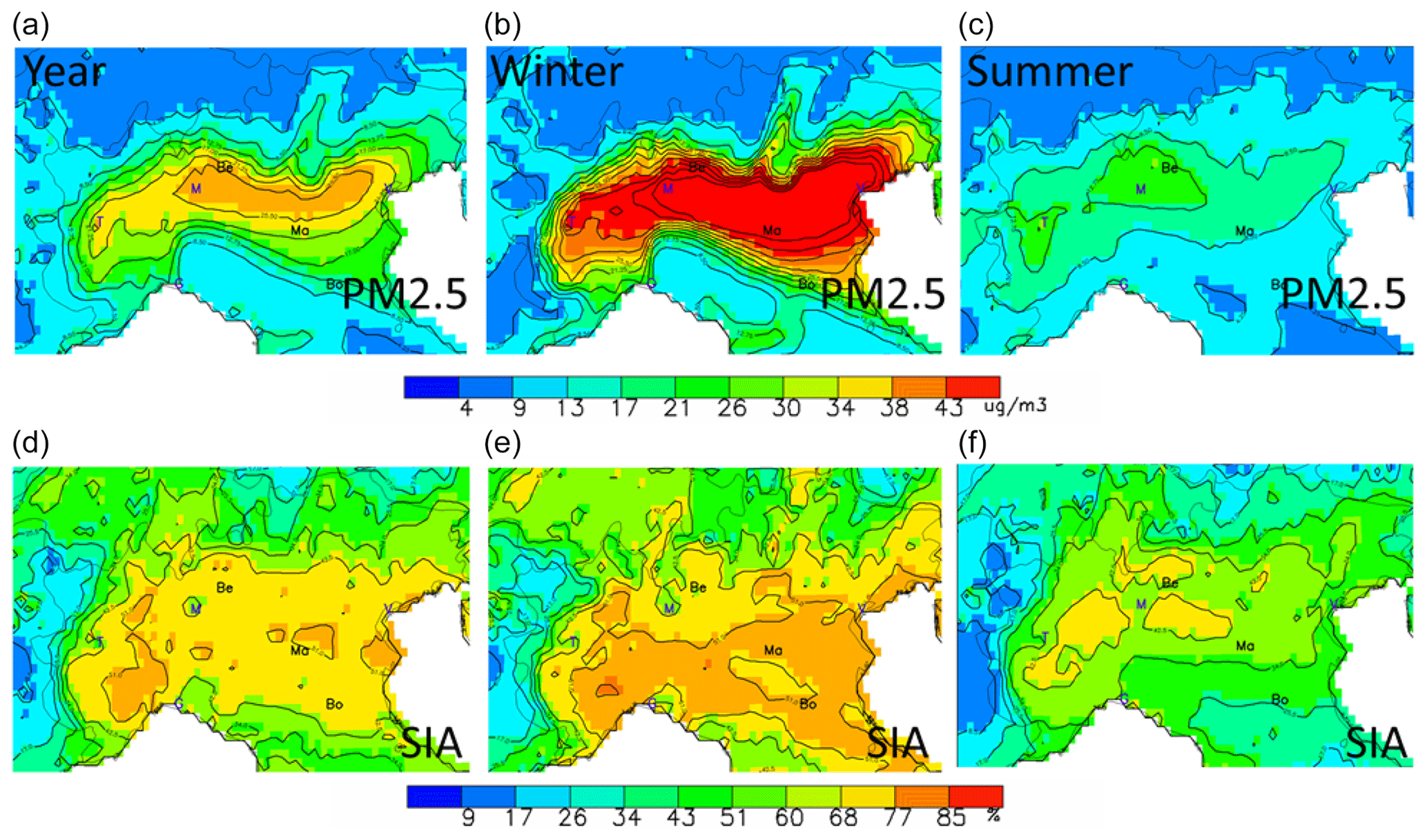
Figure 1Seasonal variations of the base-case PM2.5 (in µg m−3, a, b, c) and SIA (in percent of the PM2.5 concentration, d, e, f). The abbreviations Be, Ma and Bo represent the locations selected for more detailed analysis: Bergamo (Be), Mantua (Ma) and Bologna (Bo). Other cities are indicated by their first letter for convenience: Venice, Milan, Turin and Genoa.
In this work, we simulated a series of 24 scenarios in which NOx and NH3 emissions were reduced independently or simultaneously by 25 %, 50 %, 75 % and 100 % from the base-case reference levels. Emission reductions were applied over the entire Po basin domain for a complete meteorological year (2015).
2.2 Spatial and temporal focus
Results are generally presented in terms of maps, but three locations within the domain were selected for a more detailed analysis. The locations are Bergamo (Be) in the northern part of the domain, Mantua (Ma; also known as Mantova) in the central eastern part of the Po basin and Bologna (Bo) in its southern part. As described in the following sections, we will see that these locations show very different behaviours in terms of response to emission changes.
We also aggregate results into two seasons: winter and summer, which cover the period from November to February and from April to September, respectively. These two seasons are characteristic of different chemical regimes as illustrated in the following sections. The process to define the temporal bounds of these two seasons is discussed in Appendix A. The two remaining months (March and October) represent transition periods and are not considered in our analysis.
As we only analyse processes involving inorganic gas-phase precursors, our focus is on secondary inorganic PM2.5, although most of the results are expressed in terms of total PM2.5 concentrations. The impact of NOx emission reductions on SOA concentration is only briefly discussed in Sect. 5.
2.3 Indicators
To describe the interactions between NH3 and NOx emissions, we use the relationship proposed by Stein and Alpert (1993) and Thunis and Clappier (2014). This relation expresses the change in concentration resulting from a reduction of both precursors NOx and NH3 simultaneously, as the sum of two single concentration changes and an interaction term, as follows:
where ΔC stands for the PM2.5 concentration change (reference minus scenario) for a percentage α emission reduction (thus the term is defined as positive for a concentration reduction, consecutive to an emission reduction) and for the interaction term. We then scale each of these terms by the emission reduction (α) to generate potential impacts (P) (Thunis and Clappier, 2014).
This division by the factor α is a means to extrapolate virtually the impact resulting from any percentage emission reduction to 100 %. Potential impacts facilitate the comparison of concentration changes obtained for different emission reduction levels. Indeed, equal potential impacts imply a linear relationship between emission reductions and concentration changes. For example, for α and β, two emission reduction levels.
The overall potential impact is therefore the sum of two single potential impacts and one interaction term.
A relation between the potential impacts of combined emission reductions at two levels of intensity is obtained by writing Eq. (2) for two reduction levels α and β and subtracting the two equations. This leads to the following relation:
or equivalently via Eq. (2),
While the two first terms on the right-hand side of Eq. (4) represent the single potential impacts, the remaining right-hand side terms quantify the magnitude of non-linearities. quantifies the NOx–NH3 interaction at level α; and are the single non-linearities associated with NOx and NH3 emissions, respectively, between levels α and β; and represents the incremental change in the NOx–NH3 interaction between levels α and β.
Information about non-linearity is important to design air quality plans as it informs on the robustness of a given response, i.e. whether or not this response remains valid over a certain range and type of emission reductions. Because air quality models often provide responses for a limited set of scenarios that are then used as a basis to interpolate/extrapolate the responses to other emission reduction levels, robustness shall always be carefully assessed.
In the next section, we present the baseline results in terms of spatial and temporal variations.
Before analysing the impact of emission changes on concentrations, it is worth having a look at the baseline concentration fields. In Fig. 1, the yearly averaged PM2.5 concentration fields show a widespread pollution plume covering most of the area, with peak values extending in its central part. The maximum modelled yearly values reach 29 µgm−3, which represents an average between maximum winter values (maximum of 59 µgm−3) and minimum summer values (17 µgm−3).
The seasonal fields of PM2.5 clearly show that high yearly average values mostly result from the winter season contributions when more stable atmospheric conditions lead to stagnant conditions, favouring the accumulation of particulate matter in the area (Pernigotti et al., 2014; Raffaelli et al., 2020). The increased emissions from the residential sector (heating, especially wood burning) foster this process (Ricciardelli et al., 2017; Hakimzadeh et al., 2020). Wintertime low temperatures also favour the partitioning of semi-volatile components (e.g. ammonium nitrate) towards the particulate phase. Overall, the relative contribution of secondary inorganic particles (SIA) ranges between 40 % and 50 %, regardless of the season, and is quite homogeneously distributed spatially over the entire area. Strategies targeting SIA have therefore the potential to abate about half of the total PM2.5 concentration.
As mentioned earlier, the secondary inorganic fraction of PM2.5 results from complex atmospheric processes that involve gaseous precursors (mainly SO2, NOx and NH3), which can be summarised by the two following chemical pathways:
where (g) means gas phase, (aq) means aqueous phase, and (p) means particulate matter, and the character symbolises a chemical pathway that summarises a set of underlying reactions.
The second of these pathways (Reaction R2) is generally slower than the first one (Reaction R1), with the NO2 oxidation specific time constant being typically some hours to a day and that of SO2 being 1 to several days (Seinfeld and Pandis, 2006).
The spatial fields for the seasonal average concentrations of these precursors (Fig. 2) reflect their emission spatial patterns, resulting in a NO2-rich area that comprises Milan plus its northern districts (and to a lesser extent, Turin), while NH3 is more abundant in the central part of the Po basin, east of Milan, where intensive agriculture practices take place. Finally, high SO2 concentrations are collocated with the NO2-rich areas nearby Milan but with an additional zone around the harbour city of Genoa (also known as Genova; along the south coast), reflecting the more important SO2 emissions from the shipping sector there. However, SO2 concentrations are about 1 order of magnitude below those of NO2. Seasonal variations are well marked for NO2 and SO2 concentrations – not so much in terms of minimum and maximum values but rather in terms of spread with an extended high-concentration zone during wintertime. In contrast, NH3 concentrations remain very similar in summer and winter, both in terms of values and spatial distribution.
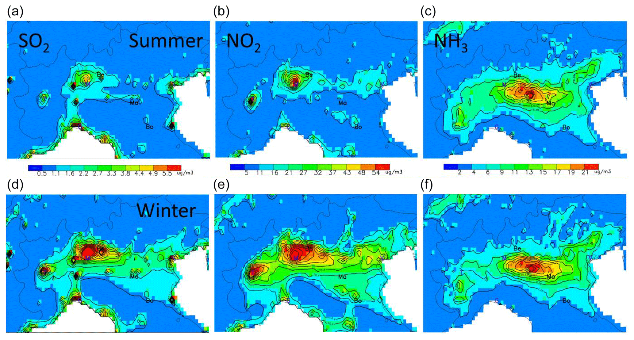
Figure 2Summer (a, b, c) and winter (d, e, f) concentration base-case fields for SO2 (a, d), NO2 (b, e) and NH3 (c, f) expressed in µg m−3. The abbreviations Be, Ma and Bo represent the locations selected for more detailed analysis: Bergamo (Be), Mantua (Ma) and Bologna (Bo). Other cities are indicated by their first letter for convenience: Venice, Milan, Turin and Genoa.
In next sections, we simulate a series of emission reduction scenarios to analyse the response of PM2.5 concentration to single and combined reductions of NH3 and NOx.
4.1 Seasonal trends
From a strategic point of view, it is important to know whether NOx (mostly emitted by the transport, industry and residential sectors) or NH3 (mostly emitted by agriculture) needs to be reduced in priority in order to reach effective results on particulate pollution mitigation. In Clappier et al. (2021), we have observed a great heterogeneity in SIA formation chemical regimes across the Po basin, with different regimes being present in limited geographical areas. Here we intend to look at these regimes in more detail.
To analyse in detail the chemical regimes in the Po basin, we compare the two single potential impacts obtained for moderate emission reductions of 25 %. Figure 3 provides a spatial overview of the difference between these two potential impacts (). This indicator tells whether reductions of NOx or NH3 will lead to the greatest PM2.5 concentration abatement, i.e. if the regime is rather NOx- or NH3-sensitive, with positive and negative values, respectively.

Figure 3Winter (b) and summer (a) chemical regimes obtained from an emission reduction level of α=25 %. The maps represent the (unit: µg m−3) indicator that shows the NOx- and NH3-sensitive areas in yellow/red and blue, respectively. The abbreviations Be, Ma and Bo indicate the location of Bergamo, Mantua and Bologna, respectively. Other cities are indicated by their first letter for convenience: Venice, Milan, Turin and Genoa.
During summertime (Fig. 3 – left), the entire area is under weak NOx-sensitive conditions with a maximum intensity in its central part, between Bergamo and Mantua.
During wintertime (Fig. 3 – right), the situation is contrasted with a wide and intense NH3-sensitive area that appears around and south-eastwards of Bergamo. This area includes big cities like Milan. Other (not as marked) NH3-sensitive regime zones appear near coastal areas. Most strongly NOx-sensitive areas are located in the eastern parts of the domain, north of Bologna and Venice. NH3-sensitive regimes are generally collocated with the NO2- and SO2-rich areas (Fig. 2), whereas NOx-sensitive regimes coincide with NH3-rich areas. The cases of the three selected cities (Bergamo, Mantua and Bologna) representative of the NH3-sensitive, NOx-sensitive and neutral regimes, respectively, are further analysed below.
The chemical regimes deducted from the results of emission reduction scenarios can be compared with the maps of the G ratio (Fig. 4), defined by Ansari and Pandis (1998) as the ratio between free ammonia (NH3 and NH) and total nitrate (HNO3+ NO) after neutralisation of H2SO4. Values of the G ratio below 1 indicate a NH3-limited chemical regime, while values above 1 characterise a HNO3-limited chemical regime.
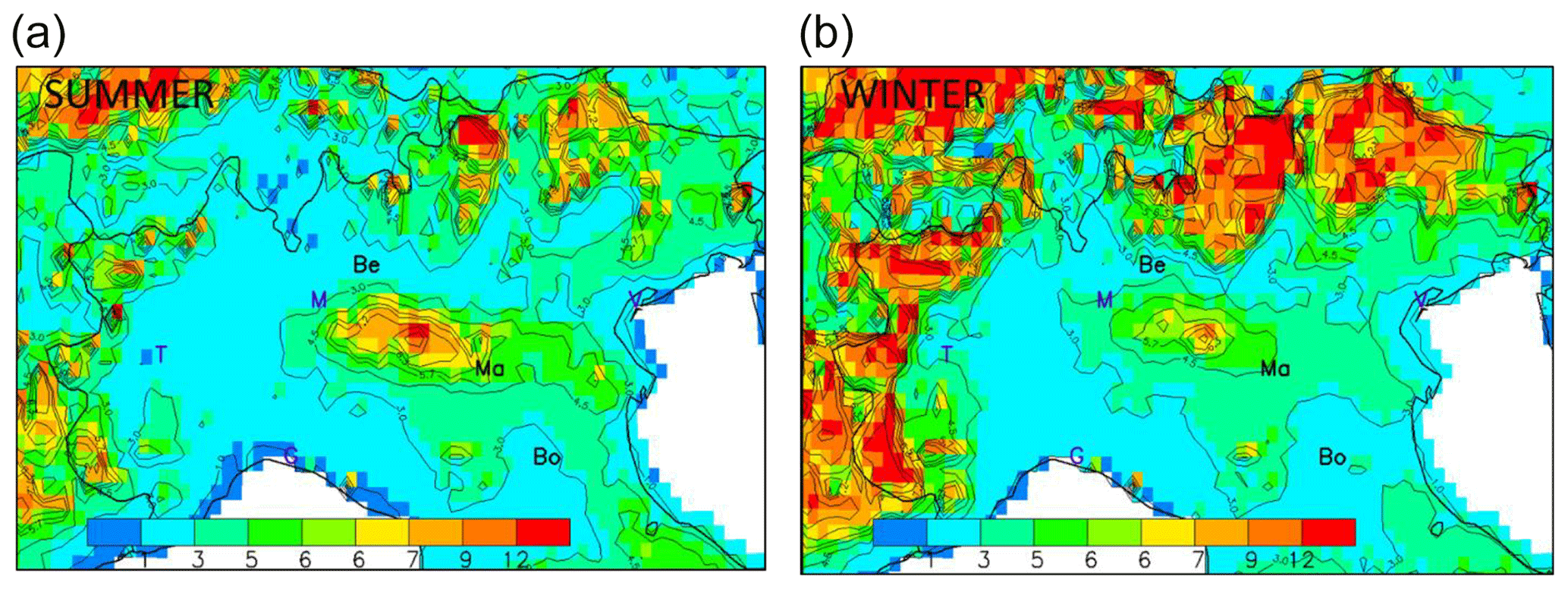
Figure 4G ratio for winter (b) and summer (a) times. The abbreviations Be, Ma and Bo indicate the location of Bergamo, Mantua and Bologna, respectively. Other cities are indicated by their first letter for convenience: Venice, Milan, Turin and Genoa.
During summer, the G-ratio values well above unity indicate a HNO3 limited chemical regime across the Po basin. This corresponds to a NOx-sensitive chemical regime in this region (Fig. 3). Moreover, the location of the G-ratio maximum between Bergamo and Mantua spatially coincides with the most pronounced NOx-sensitive regime and to a maximum of NH3 concentrations of about 20 µg m−3 (Fig. 2). Indeed, NOx emission reductions lead to HNO3 concentration reductions, which is the limiting factor in NH4NO3 formation according to the G ratio. During winter, the G ratio still shows large values in the region south-east of Bergamo, but, contrary to summer, the chemical regime is clearly NH3-sensitive (Fig. 3). More generally, G-ratio values remain above unity over the whole Po basin, while both NOx- and NH3-sensitive chemical regimes prevail in different areas. Therefore, the G ratio, related to the abundance of total free ammonia and total nitrate, provides information which differs from that obtained by determining the distribution of the NH3- and NOx-emission-sensitive chemical regimes. These differences illustrate the impossibility to directly use the G ratio for air quality management, an interesting result in itself. We will further discuss this interesting behaviour later when addressing non-linearity in Sect. 4.3.
4.2 Impact of the emission reduction strength
In this section, we repeat the analysis of Sect. 4.1 for yearly average concentrations but looking at the step changes of regimes as we progressively reduce emissions from the base-case situation. (Fig. 5). Chemical regimes are well in place for a 25 % level reduction (top left) and are only slightly perturbed from 25 % to 50 % with a reinforcement of the NOx limited regime (top right). Despite this slight change in intensity, the regimes therefore keep the same spatial patterns. From 50 % onward, chemical regimes tend to attenuate and reverse themselves from 75 % to 100 % (bottom right).
In other words, locations that are NH3-sensitive for the first steps emission reductions will become NOx-sensitive for the last steps emission reductions, and vice versa.
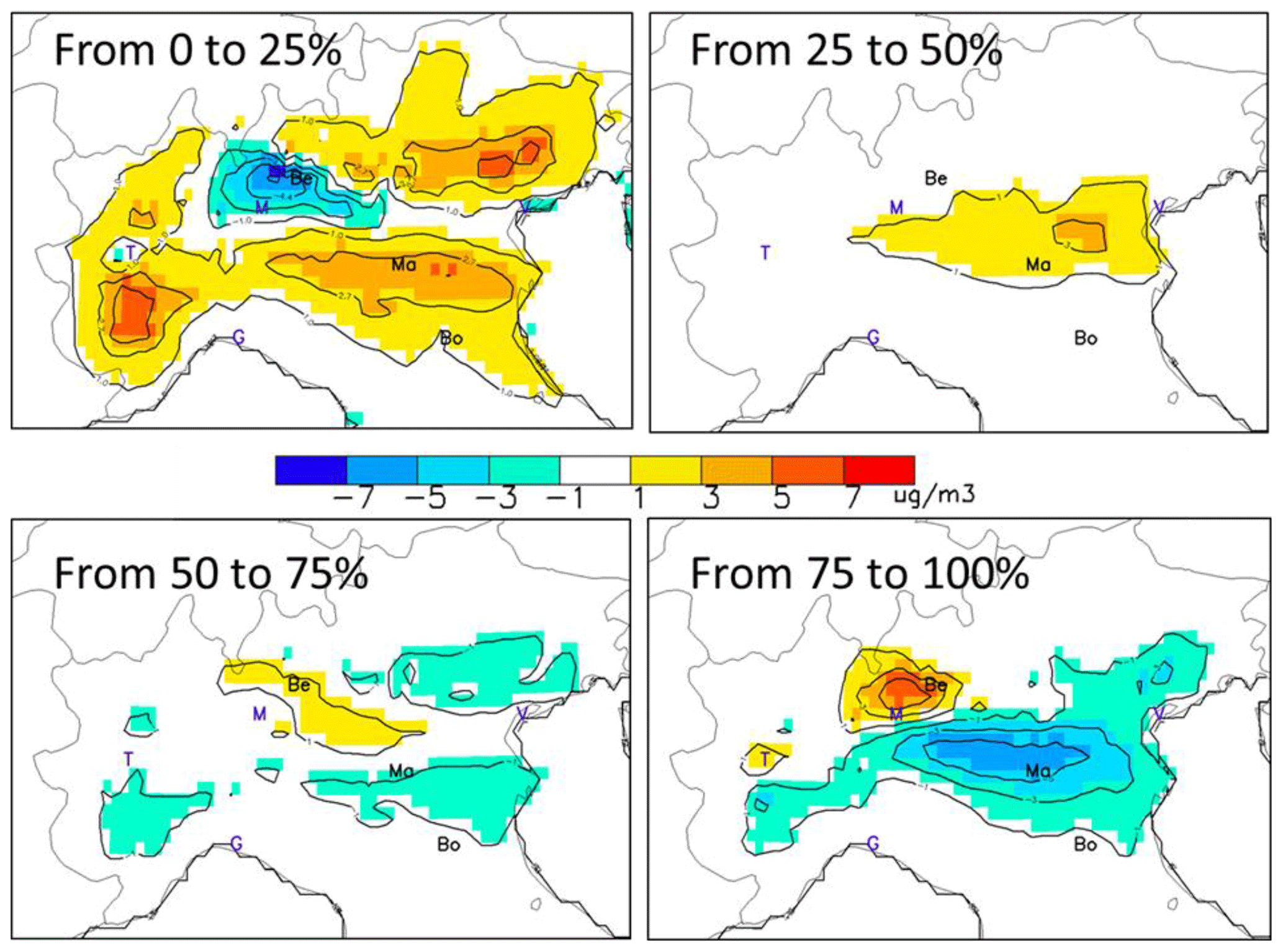
Figure 5Yearly averaged chemical regimes obtained from a 25 % emission reduction starting at different levels of emissions corresponding to α=0, 25, 50 and 75. The maps represent the () between the starting and ending levels (unit: µg m−3) showing the NOx- and NH3-sensitive areas in yellow/red and blue, respectively. The abbreviations Be, Ma and Bo indicate the location of Bergamo, Mantua and Bologna, respectively. Other cities are indicated by their first letter for convenience: Venice, Milan, Turin and Genoa.
4.3 A summarised overview: the PM2.5 isopleths
Like isopleth plots that show the variations in the O3 concentrations as a function of NOx and VOC concentrations (Dodge, 1977), similar plots can be created for PM2.5 concentrations as a function of NOx and NH3 emissions. Simulation results have indeed often been presented as 2D isopleths of PM2.5 or nitrate as a function of precursor emissions, which allows showing in a comprehensive manner their sensitivity and also in a qualitative manner non-linear effects (for example Watson et al., 1994, over the USA; and Xing et al., 2018, over the Beijing–Tianjin–Hebei region in China). Figure 6 shows the PM2.5 isopleths obtained through an interpolation among the 25 simulation concentration values (these 25 simulations correspond to the white square symbols in each isopleth diagram) at the three locations Be, Ma and Bo previously defined. The x and y axes represent the strengths of the NH3 and NOx emission sources, respectively. With this type of graphical representation, it is possible to visualise the response of PM2.5 to a NOx emission change by moving vertically, the reaction to a NH3 emission change by moving horizontally or the reaction to a combined NOx–NH3 emission change by moving diagonally. The larger the number of isopleths we cross on the path (high gradient), the larger the expected impact from an emission reduction will be. A simple theoretical model to generate and interpret these isopleths is proposed in Appendix B.
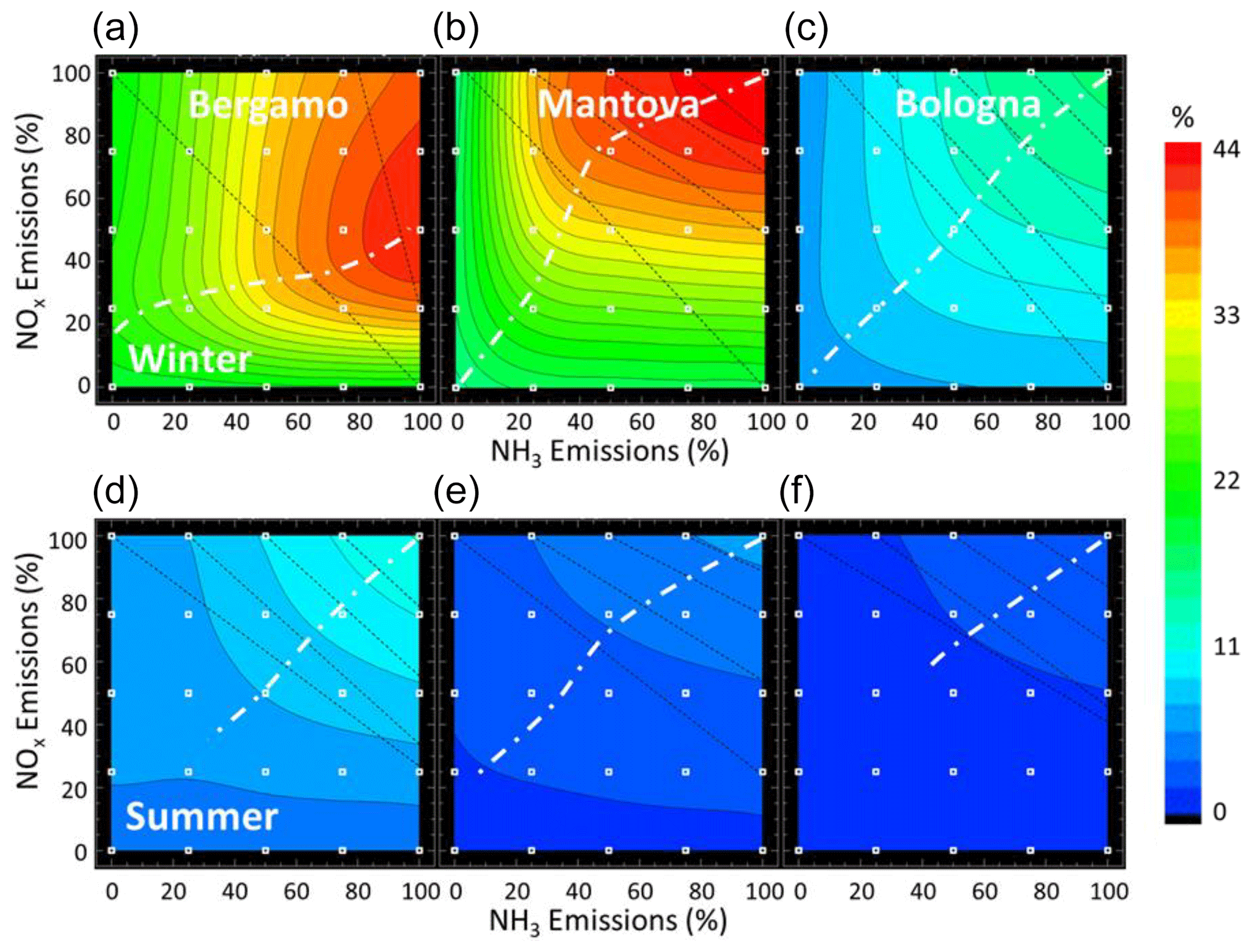
Figure 6PM2.5 isopleths during winter (a, b, c) and summer (d, e, f) at the three locations of interest (see maps). PM2.5 concentrations are expressed in µg m−3 as a function of the intensity of the NOx (y axis) and NH3 (x axis) emissions, respectively. The overlaid dashed oblique lines on each diagram connect similar PM2.5 concentration values for single NOx and NH3 reductions. The more vertical these lines are, the larger the NH3 abatement impact compared to the NOx abatement impact is; the more horizontal they are, the larger the NOx abatement impact compared to the NH3 abatement impact is. The dashed line delineates the ridge between the NH3- and NOx-sensitive areas.
From the analysis of the isopleths, we note the following points.
-
In general, the isopleths show a regular pattern with a progressive decrease in PM2.5 concentration when either the NOx or NH3 emissions are reduced, with the only exception being Bergamo during wintertime, where NOx reductions up to 70 % lead to a small increase in PM2.5 (Fig. 6 – top left), whatever the reduction in NH3 emission is. We discuss this particular feature later in this section.
-
The diagram areas can be divided into two zones separated by a ridge (dashed line in Fig. 6). Above the ridge line, PM2.5 is more sensitive to NH3, while below the ridge line, it is more sensitive to NOx emission reductions. The orientation of the ridge (tending to vertical or horizontal) informs on the type of chemical regime (NOx- or NH3-sensitive, respectively).
-
The efficiency of a NOx vs. NH3 emission reduction varies across locations. We can compare the efficiency of a given reduction by looking at the horizontal (for NOx) and vertical (for NH3) gradients. To support this comparison, we included in each diagram dashed oblique lines that connect similar PM2.5 concentration values for single NOx and NH3 emission reductions. The more vertical these lines are, the larger the NH3 abatement impact compared to the NOx abatement impact is. Conversely, the more horizontal they are, the larger the NOx abatement impact compared to the NH3 abatement impact is. For moderate emission reductions (up to 50 %, top-right corner), different behaviours are observed: while in Bergamo PM2.5 is more sensitive to NH3 reductions, it is more sensitive to NOx reductions in Mantua, and it is equally sensitive to both precursors in Bologna. This corresponds to the spatial patterns of NOx- and NH3-sensitive regimes depicted in Fig. 3.
-
Winter- and summertime isopleths show completely different patterns in Bergamo, whereas at the two other locations, they remain similar.
-
At Mantua where moderate NOx reductions (e.g. 50 %) are the most efficient among the three sites, NH3 emission reductions are more efficient than NOx emission reductions for larger additional reductions (going for example from 75 % to 100 %). At Bergamo, NH3 reductions are the most effective for moderate reductions, whereas NOx reductions become more effective for larger reductions, as seen by the isopleths spacing. This confirms the finding of reversed chemical regimes for larger additional emission reductions detailed in the previous section and illustrated in Fig. 5.
The special pattern of Bergamo's PM2.5 isopleths during wintertime needs some additional discussion. The increase in the inorganic fraction of PM2.5 as a response to NOx reductions during wintertime has already been noted by several authors (e.g. Le et al., 2020; Sheng et al., 2018). It has been related to an increase in the oxidising capacity of the atmosphere and in particular to increased ozone levels. This is due to the prevailing titration of O3 by NO in wintertime high-NOx conditions and in the absence of photochemical ozone production due to reduced solar radiation (Kleinman et al., 1991).
The impact of NOx emission reductions on the concentration of various pollutants in Bergamo during wintertime is illustrated in Fig. 7. As expected, a 50 % reduction in NOx emissions leads to a decrease in NO2 concentration (from 47 to 28 µg m−3, i.e. a factor of 1.7). In contrast, O3 concentration increases from 8 to 16 µg m−3, roughly a factor of 2. These compensating changes result in a small increase in NO3 radical production (Reaction R4), which is the initial step of the major pathway of wintertime HNO3 and particulate nitrate formation (Kenagy et al., 2018).
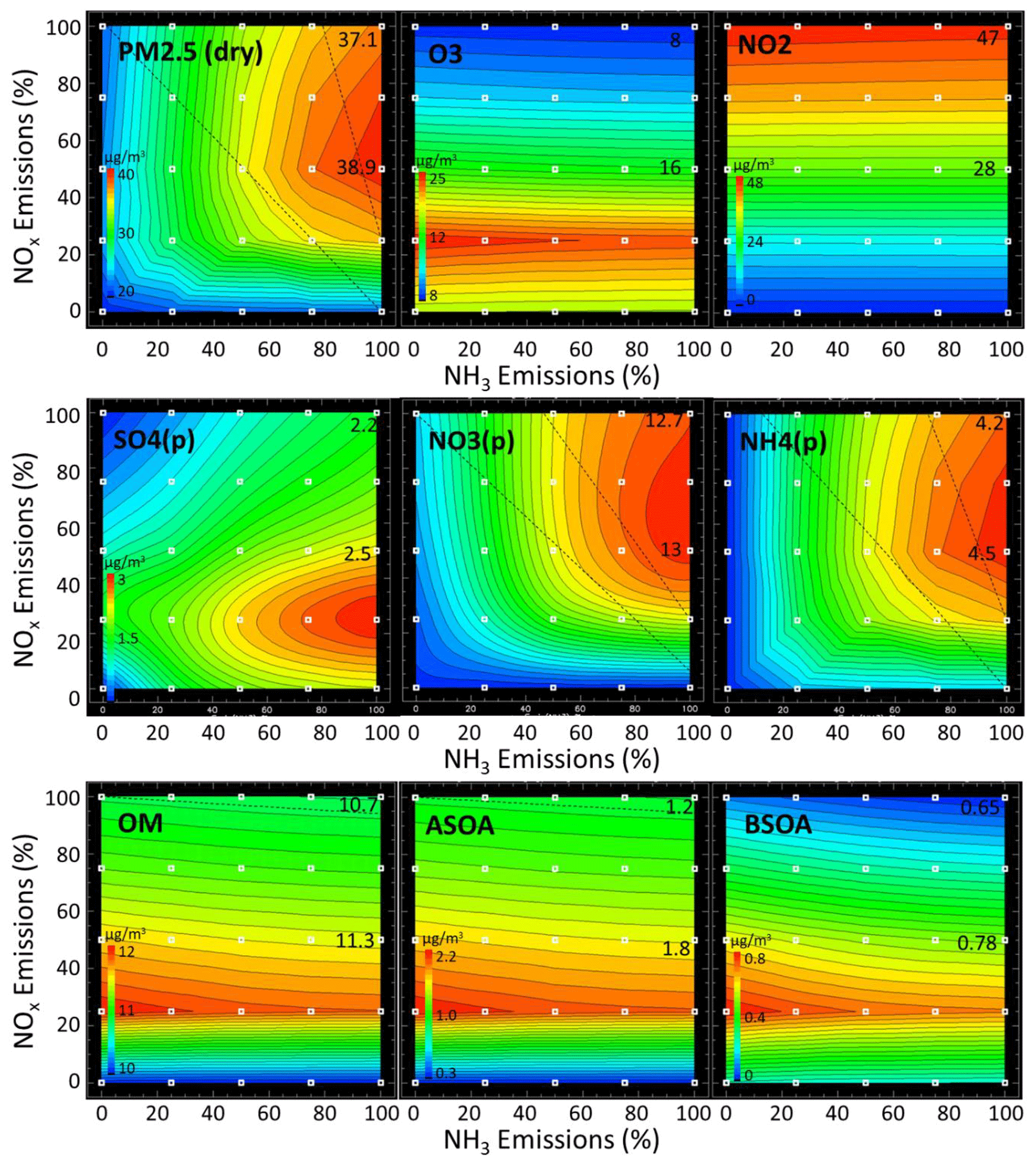
Figure 7Wintertime isopleths in Bergamo for the species: dry PM2.5, O3, NO2, sulfate (SO4), nitrate (NO3), ammonium (NH4), organic matter (OM), and anthropogenic and biogenic secondary aerosols (ASOA and BSOA, respectively). The two numbers on the vertical axis indicate concentration values for the base case and at the 50 % NOx emission level.
In this pathway, the NO3 radical formation is followed by combination with NO2 to form N2O5, a reversible process, and heterogeneous HNO3 formation on wet particle surfaces.
The NO3 radical has three major rapid sinks: reaction with NO, photolysis, and reaction with NMVOCs, especially terpenes.
Reactions (R3) to (R10) induce additional dependence of HNO3 formation on NOx species on top of Reaction (R1), but which partly cancel out, as they are both involved in formation and sink processes.
SOA is formed through a series of chemical reactions of gaseous precursors – mainly volatile, intermediate volatility or semi-volatile organic compounds (VOCs) with the oxidants O3, OH and nitrate radical (NO3) (Li et al., 2011).
Putting all the arguments together, it follows that wintertime ammonium nitrate formation over Bergamo is most probably controlled by NO3 radical formation (Reaction R4). The fact that this behaviour is observed in Bergamo and not in Mantua or Bologna is due to the much larger NO2 levels in the Bergamo–Milan area (above 50 µg m−3 during winter, Fig. 2). Such large NO2 levels are also simulated locally over the Turin area and also lead to a slightly NH3-sensitive regime there despite a G ratio well above unity. Beyond 50 % NOx reduction, NH4NO3 formation decreases because NO2 decreases more rapidly than ozone increases up to its maximum (at 75 % NOx emission reduction; see Fig. 7).
The negative response of NH4NO3 to NOx emission reductions in Be during wintertime explains the apparent discrepancies with the analysis of G ratio, which indicates that NH4NO3 is strongly HNO3 limited. Simply, the HNO3-limited chemical regime cannot be extrapolated to sensitivity to NOx emissions in the case of the above shown negative response. Total nitrate is less abundant than free ammonia (defined as , but NOx emission reductions up to about 50 % do not reduce its concentration, and NH3 emission reductions are thus more efficient. In this respect, the G ratio cannot provide information about negative responses.
At Bergamo during winter, the increase in PM2.5 (+1.8 µg m−3) arising from a 50 % reduction in NOx emission also results from an increase in sulfate (+0.3 µg m−3) and in SOA (+0.6 µgm−3) concentrations. Both sulfate and SOA concentrations are closely related to O3 concentrations (Fig. 7). The sulfate increase is comparable in magnitude to the nitrate increase, even if sulfate levels are much smaller than nitrate ones. Figure 7 actually shows a strikingly similar response of sulfate, SOA and ozone to NOx emission reductions (given that SO2 and NMVOC emissions are held constant). Indeed the prevailing wintertime aqueous production of H2SO4 requires oxidants and in particular ozone (Le et al., 2020; Sheng et al., 2018). In addition, the formation of SOA in both the gas and particulate phases also requires oxidants (Vahedpour et al., 2011; Huang et al., 2020; Feng et al., 2016, 2019; Li et al., 2011; Tsimpidi et al., 2010).
Pinder et al. (2008) also note an oxidant limitation for SIA formation over the eastern United states for the 2000 to 2020 period, but in their simulations, it mainly affects sulfate that increases as a result of NOx emission reductions while nitrate decreases. This is due to a more important sulfate-to-nitrate ratio in the eastern United States than over the Po basin. Fu et al. (2020) derive from combined measurements and modelling that wintertime nitrate during haze events in the North China Plain (NCP) is nearly insensitive to 30 % NOx emission reductions, because increased ozone levels increase the NOx to HNO3 conversion efficiency. Following these authors, this conversion also involves the homogeneous HNO3 formation via the NO2+OH. This reaction also could play a role in the Po basin, in addition to the heterogeneous pathway. Also Leung et al. (2020) simulate that wintertime nitrate abatement in the NCP is buffered with respect to emission reductions by increased oxidant build-up but also by sulfate to nitrate conversion by liberating free NH3 through sulfate concentration reduction, which can then enhance nitrate formation. Womack et al. (2019) find an oxidant limitation of nitrate formation over wintertime Utah (USA) and show that nitrate concentration diminishes when reducing VOC emissions.
Clappier et al. (2021) highlighted the specificities of the Po basin area within Europe. They showed that non-linearities are present in this region. One peculiarity of the Po basin is a marked difference between the chemical regimes encountered within a confined area, which have implications on the linearity of PM2.5 responses to emission changes. In this section, we analyse in more details these non-linearities.
Information on the NOx–NH3 interaction term at the reduction level α=25 %, (first non-linear term in Eq. 4), is provided in Fig. 8. At α= 25 %, the interaction term is negative (or null) across the entire modelling domain (most data points are below the 1:1 line) regardless of the chemical regimes and averages to approximately −10 %, as indicated by the linear fit slope (=0.9). In relative terms, this interaction term is also almost constant regardless of the season (not shown).
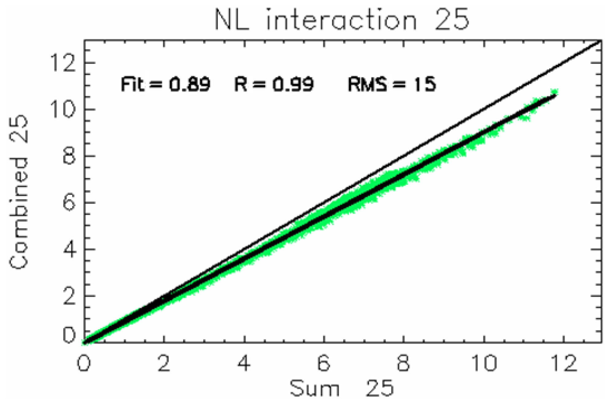
Figure 8Yearly mean non-linear interaction term for a 25 % reduction in NOx and NH3. The scatter plot compares the sum of the potential impacts of the two single reductions (x axis) with the potential impact of the combined emission reduction (unit: µg m−3) (y axis). Departure from the 1:1 line quantifies the overall non-linearity. Each data point represents the yearly average values for a grid cell in the modelling domain.
This negativity can be explained by the fact that a reduction of only NOx implies a reduction of both and , and the same happens when reducing only NH3; therefore a simultaneous reduction of both precursors is lower than the sum of the two. Single impacts would therefore lead to an overestimation (of about 10 %) in PM2.5 reduction if added up to extrapolate linearly the impact of combined 25 % NOx and NH3 emission reductions on yearly averaged PM2.5 concentrations. This result is expected for what concerns particulate NH4NO3, as a consequence of the gas–particle equilibrium described in Reaction (R1), although non-linear relationships between NOx emissions and HNO3 concentrations also play a role. Qualitatively, this negative interaction is also highlighted by the hyperbolic shapes of the PM2.5 isopleths determined for three different sites of the domain (Fig. 6). As discussed in Appendix B, linearity would result in isopleths parallel to the descending diagonal lines.
When emission reductions increase from 25 % to 50 %, three additional non-linear terms are generated (three last terms in Eq. 4). Figures 9 and 10 provide an overview of these non-linear terms during wintertime and summertime, respectively. The top-left panel of each figure represents their sum, i.e. the total non-linearity generated between 25 % and 50 % emission reduction. The right column shows the non-linearities associated with NOx and NH3, while the bottom-left panel reports the non-linear interaction between the two precursors.
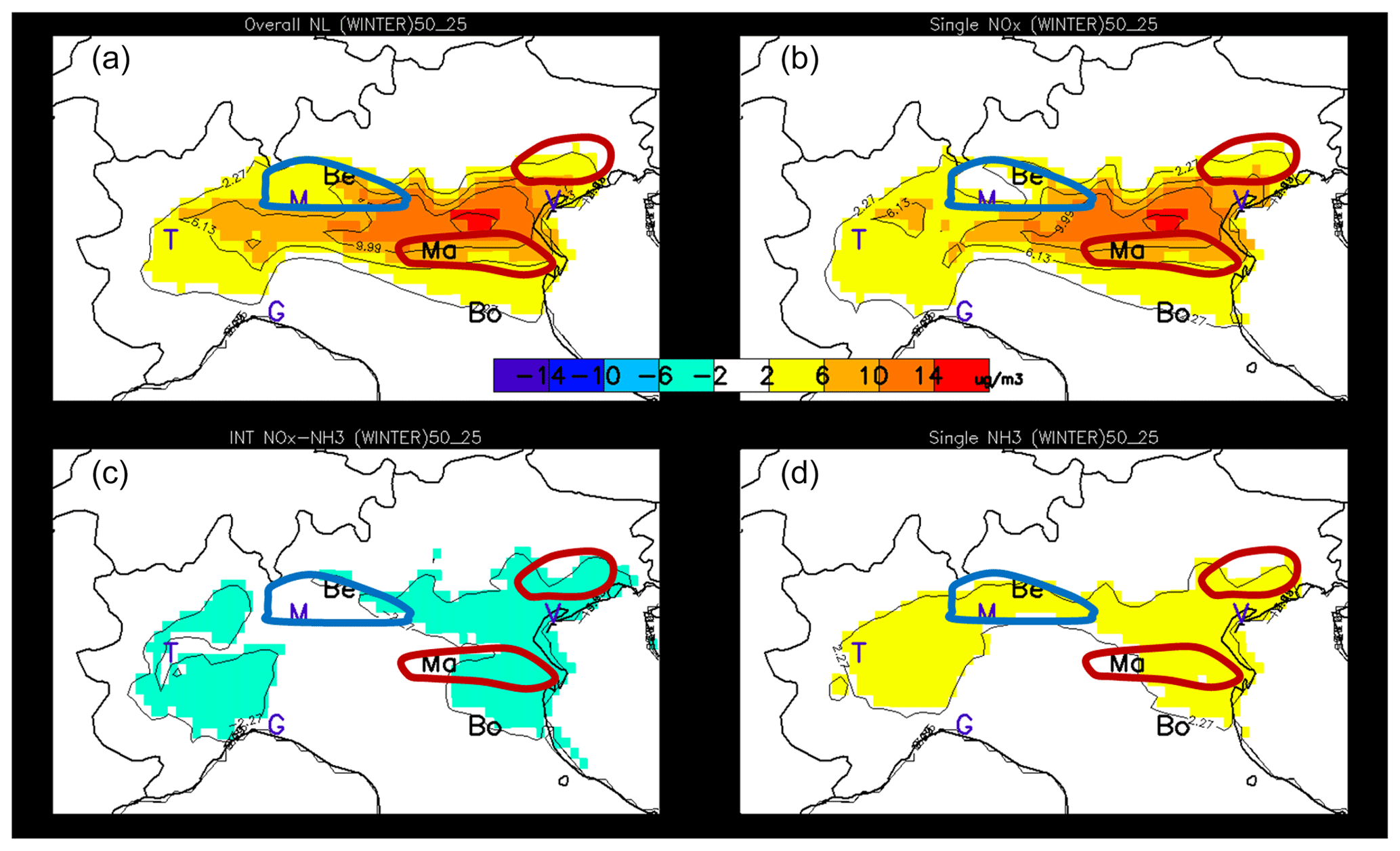
Figure 9Wintertime maps of the overall non-linearity term (a) and of its components expressed as potential impacts between 25 % and 50 %: the single NOx non-linearity term (a, b), the single NH3 non-linearity term (d) and the NOx–NH3 interaction term (c). The three locations of interest, Bergamo, Mantua and Bologna, are indicated by their first two letters, while other cities are indicated with their first letter for convenience (Venice, Milan, Turin and Genoa). The hand-drawn contours roughly indicate the central position of the NH3 (blue) and NOx (red) sensitive regime areas (see Fig. 3 – right).
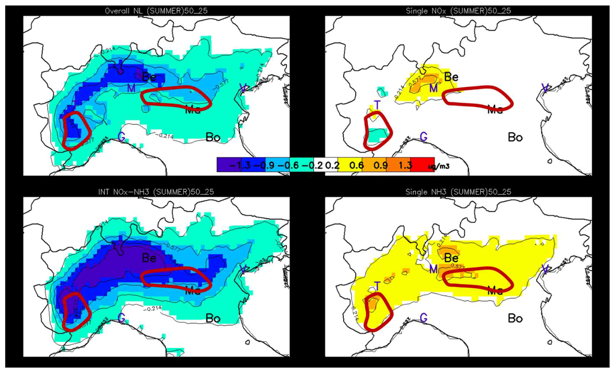
Figure 10Same as Fig. 9 but for summertime.
Overall, non-linearities are more important during wintertime than during summertime. This is true both in absolute and relative (not shown) terms. Non-linearities tend to be the largest in between areas that are characterised by well-marked NH3- or NOx-sensitive regimes (indicated by the blue and red drawn contours). This can be explained by the fact that when one of the two components (NOx or NH3) is in large excess (compared to the other one), reductions of this compound have then generally only little impact, implying that both single and combined reductions only involve one compound and are therefore similar.
During wintertime, the overall non-linearity (Fig. 9 top left) is largely dominated by the single NOx-related non-linearity (, Fig. 9 top right) – a singularity in Europe as the Po basin is the only area where this occurs to this extent (Clappier et al., 2021). In the region of Bergamo, the NOx non-linearity remains weak despite the peculiar PM2.5 responses to NOx emission reductions (i.e. an increase in PM2.5 concentrations for NOx emission reduction up to 50 %, Fig. 7). In this NH3-sensitive region, this behaviour can be explained by the strong oxidant limitation of HNO3 formation outlined above (Fig. 7). It is worth mentioning that, although atypical, this behaviour is quasi-linear with PM2.5 responses that remain proportional to the emission reduction strength (up to 50 %) but with a negative slope. Similarly to NOx, NH3 single non-linearities (Fig. 9, bottom right) are positive but weaker, indicating slightly larger potential impacts for emission reductions in the range 25 %–50 % than in the 0 %–25 % range. Finally, the NOx–NH3 non-linear interaction terms (Fig. 9, bottom left) are mostly negative, indicating that the interaction term for 50 % emission reductions is more negative than the corresponding term for 25 %, pointing out to a strengthening of the NOx–NH3 non-linearity when more intense emission reductions are considered.
In relative terms, the overall wintertime non-linearity terms increase by about 30 % when emission reductions increase from 25 % and 50 % (Fig. 11 top, blue points). Note that these non-linearity terms reach larger values in some places of the modelling domain as highlighted by the data point dispersion. In a previous work, Thunis et al. (2015) quantified the non-linearity of model responses to emission reductions in three areas in Europe, among which is the Po Basin. One of their conclusions was that non-linearities remain relatively low for yearly averaged responses. Although the results presented here show important non-linearities, these occur mainly during wintertime and are limited to specific areas. It is also worth noting that these non-linear responses (for moderate emission reductions up to 50 %) only occur in the Po Basin (Clappier et al., 2021).

Figure 11Changes in the overall non-linearity terms from 25 % to 50 % (a), from 50 % to 75 % (b) and from 75 % to 100 % (c) in NOx and NH3. The overall non-linearity is visualised as the distance from the 1:1 diagonal, i.e. the difference between the overall potential impact at two levels of emission reduction, x and y axis. Each point represents one land grid cell within the domain for wintertime (blue) and summertime (red). The “fit” parameter indicates the slope of the regression line, while R2 and RMS provide information on the coefficient of determination and the root mean square error, respectively.
During summertime, the magnitude of non-linear terms is smaller than during wintertime. The overall non-linearity term (top left) is dominated by the NH3–NOx non-linear interaction term (, Fig. 10, bottom left). In summer, the PM2.5 concentration is NOx-sensitive in almost all the domain (Fig. 3), and emission reductions do not lead to shifts in the chemical regimes. In this case, the interaction terms become more important. The non-linear interaction terms are negative everywhere in the Po basin, implying again that the interaction terms at 50 % are more negative than at 25 % emission reduction (reinforcement of the non-linearities when more intense emission reductions are considered). Most negative values appear in the western and northern part of domain.
Figure 11 shows the increase in the overall non-linear terms for emission reduction steps starting from different points, from 25 % to 50 %, from 50 % to 75 % and finally from 75 % to 100 %. Regardless of the emission reduction step, summertime non-linearities remain small all over the domain, with the regression slope close to 0.9 and very limited data point dispersions (i.e. low RMSE). Wintertime non-linearities further increase significantly from 50 % to 75 % reduction levels (regression fit parameter close to 1.21) but tend to stabilise between 75 % and 100 % reduction levels (regression fit parameter close to 1.05). It is interesting to note that potential impacts in winter increase for all segments (all winter points are above the 1:1 line), indicating that the same percentage reduction (25 %) gains progressively more impact when more intense reductions are considered.
When designing air quality plans, it is important to identify the key precursors on which to act in priority to hit a specific air quality target but also to understand the consequences of these choices for various seasons (temporal variations), locations (spatial variability), emission reduction levels (strength) and strategies (combined or single emission reductions). As the information to make this decision is generally incomplete, assessing the robustness of the available model responses is essential. From the results presented here, a few key points appear.
The seasonal and spatial variabilities in the response of PM2.5 to the reduction of NOx and NH3 emissions are extremely large, with different and sometimes opposite responses to emission changes. Yearly averages do not represent the appropriate time window to evaluate the impact of such emission reductions, and a focus on wintertime (November to February) seems to be the right option, especially because concentrations are larger during this period of the year.
The responses of PM2.5 to emission reduction plans that cover the whole area (i.e. uniform emission reductions are applied everywhere in the domain) vary from location to location: opposite responses occur within a few hundred kilometres for some reduction levels. In the region of Bergamo, the PM2.5 response to NOx emission reductions can be negative, meaning an increase in PM2.5 when reducing the NOx emissions. It is important to combine NOx and NH3 emission reductions in winter or to go for stronger emission reductions to make sure these unwanted effects are limited.
Despite quite important non-linearities, PM2.5 responses to emission reductions are not chaotic. Indeed, regardless of the emission reduction level, the non-linear terms related to NH3 emission reduction and to NOx–NH3 interactions are quite uniform spatially. This is not the case of NOx emission reduction, for which care must be taken to ensure that the detailed response of PM2.5 is captured.
Although they are location specific, PM2.5 isopleths represent an interesting tool to assess the impact of different NOx and NH3 emission reductions on PM2.5 concentration. They indeed allow visualising in one single diagram the impact of any type of reductions on concentrations in a single grid cell (or set of grid cells). We must however remember that these isopleths derive from uniform emission reduction over the whole domain. Comparing sites where PM2.5 responses to the same “domain-wide” policy are different, it appears challenging to define a single domain-wide policy efficiently reducing PM at all locations.
In this work, we analysed the sensitivity of PM2.5 to NOx and NH3 emissions by means of a set of EMEP simulations performed with different levels of emission reductions, from 25 % up to a total switch-off of those emissions. Both single and combined precursor reduction scenarios were applied to determine the most efficient emission reduction strategies and quantify the interactions between NOx and NH3 emission reductions. Our results confirm the peculiarity of secondary inorganic PM2.5 formation in the Po basin suggested by Clappier et al. (2021), characterised by contrasting chemical regimes within distances of a few (hundred) kilometres, as well as non-linear responses to emission reductions during wintertime. One of the striking results is the increase in the PM2.5 concentration levels when NOx emission reductions are applied in NOx-rich areas, such as the surroundings of Bergamo. The isopleths in the graphs showing PM2.5, nitrate, sulfate, SOA and O3 concentrations as a function of NH3 and NOx emissions (Fig. 7) indicate that the increased oxidative capacity of the atmosphere is the cause of the increase in PM2.5 induced by a reduction in NOx emission of up to 50 %. This process can have contributed to the absence of significant PM2.5 concentration decrease during the COVID-19 lockdowns in many European cities (EEA, 2020; Putaud et al., 2021). It is important to account for this process when designing air quality plans, since it could well lead to transitionary increases in PM2.5 at some locations in winter as NOx emission reduction measures are gradually implemented. At this type of location, mitigation measures that would be optimal in the long term might not be efficient in the short term.
Joint analyses of PM sensitivity to emissions and the G ratio can give a clue if a NH3-sensitive chemical regime is due to either a lack of NH3 or to a non-linear and negative response of HNO3 concentration to NOx emissions. In this latter case, the chemical regime is NH3-sensitive in terms of NH3 and NOx emission reductions, but it can be HNO3 limited in terms of the G ratio, as observed for the Bergamo–Milan region. Inversely, a G ratio greater than 1, indicating HNO3 limitation to particulate nitrate formation, does not necessarily indicate a larger sensitivity to NOx than to NH3 emissions. Thus, our results show the impossibility to directly use the G ratio for air quality management, an interesting result in itself. While PM2.5 chemical regimes (determined by the relative importance of the NOx vs. NH3 responses to emission reductions) show large variations seasonally and spatially, they are not very sensitive to moderate (up to 50 %) emission reductions. Beyond 25 % emission reduction strength, responses of PM2.5 concentrations to NOx emission reductions become non-linear in certain areas of the Po basin mainly during wintertime.
Since sulfate concentrations are low in the Po basin, the impact of SO2 emission reductions was not evaluated here. However, the simulations performed in Clappier et al. (2021) indicate that air quality improvement plans addressing SO2 emissions may still lead to additional PM2.5 decreases. Further works should also test if NMVOC emission would further affect the concentration of oxidants and subsequently of nitrate (and sulfate) during winter. This depends on the fraction of ozone formed photochemically in the Po basin, compared to the one transported from outside by advection or entrainment.
Finally, it would be important to compare the results obtained in this work from the EMEPrv4_17 model with similar results obtained from other models. With its complex setting, the Po basin represents a good test case for such inter-comparisons.
Chemical regimes show a great variability with time. To select the extension of the seasons, we analyse the monthly behaviour of the NH3 and NOx responses as well as the interaction terms (Fig. A1). The analysis is performed for two locations: Bergamo, which lies in a NH3-sensitive zone; and Mantua, which lies within a NOx-sensitive zone. On these plots, we identify two major seasons with a consistent behaviour: winter from November to February and summer from April to September. These two seasons are similar at both locations. The two remaining months, March and October, are transition months and are not considered in the analysis. It is interesting to note that these two transition periods correspond more or less to the switching time between the NOx and NH3 concentration time profiles (Fig. 12 – right panel). On the latter figures, the SO2 and NO2 temporal evolutions are almost identical, in contrast to NH3.
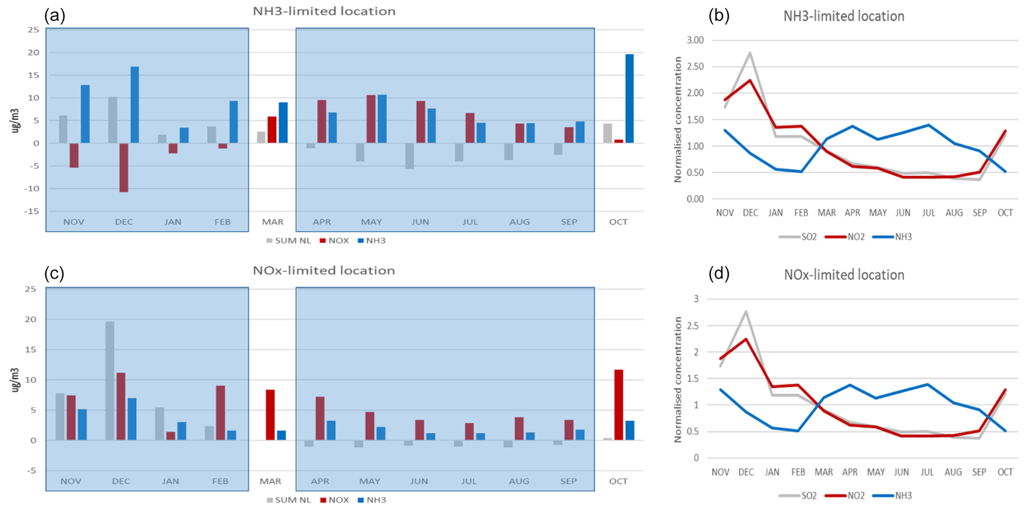
Figure A1Monthly averaged responses to NH3 (blue), NOx (red) reductions (25 %) and interaction terms (grey) at two locations: Bergamo (a, b) and Mantua (c, d). Panels (b) and (d) shows the monthly evolution of the concentrations of NO2, NH3 and SO2 at those two locations. Note that concentrations are normalised by their average values.
To facilitate the interpretation of the isopleths diagrams, we use a simple theoretical example that mimics the complex reactions process schematised by Reactions (R1) and (R2) above. Our simplified process is described by the following relation: , where Cc is the concentration of a compound “c” that is given by the minimum between two emitted species A and B. The concentration depends on the strengths of these emissions, specified by the parameters x and y. For each emission strength (x or y), the two emission species are proportional to their full-scale value (100 %): EA(x)=xEA[100] and EB(y)=yEB[100], respectively. If we choose EA(100)≫EB(100), we create a B-sensitive environment (Fig. B1 – left column) and inversely (Fig. 13 – right column). If we select mixed situations, representing for example an average of days, during which we alternate between A- and B-sensitive regimes, we obtain the two bottom isopleth diagrams that represent cases where a larger number of A-sensitive (right) or B-sensitive (left) events are recorded. Although extremely simple, these diagrams illustrate properties that are observed on the real test cases.
Let us take the example of an A-sensitive regime. Similar observations can be made in the case of a B-sensitive regime. We note the following points.
-
The diagram area can roughly be divided into two zones separated by a ridge: a top-left triangle where the sensitivity to emission reductions of species “B” dominates and a bottom-right triangle where the sensitivity to A dominates. The slope of the ridge (larger or less than 1) informs on the type of regime.
-
In the case of a single A-sensitive day (top right) with EB(100)=2EA(100), the concentration of compound “c” remains unchanged for emission reductions of B up to 50 %, while its concentration react in a linear way to emission changes in A from 0 % to 100 %. Between the base case and a reduction level of 50 %, the A gradient is therefore larger than the B gradient. This implies that the B gradient is larger than the A gradient between the 50 % and 100 % reduction levels because we know that for a 100 % reduction of A or B, the concentration must be zero. In our simple example, the gradient of B is zero from 0 % to 50 % but is twice as large as A between 50 % and 100 %.
-
While the combination of several events (e.g. days) characterised by different regimes leads to smoother isopleths (bottom), the same characteristics can be noted. In particular, the inclination (tending to the horizontal or vertical) provides information on the type of chemical regime.
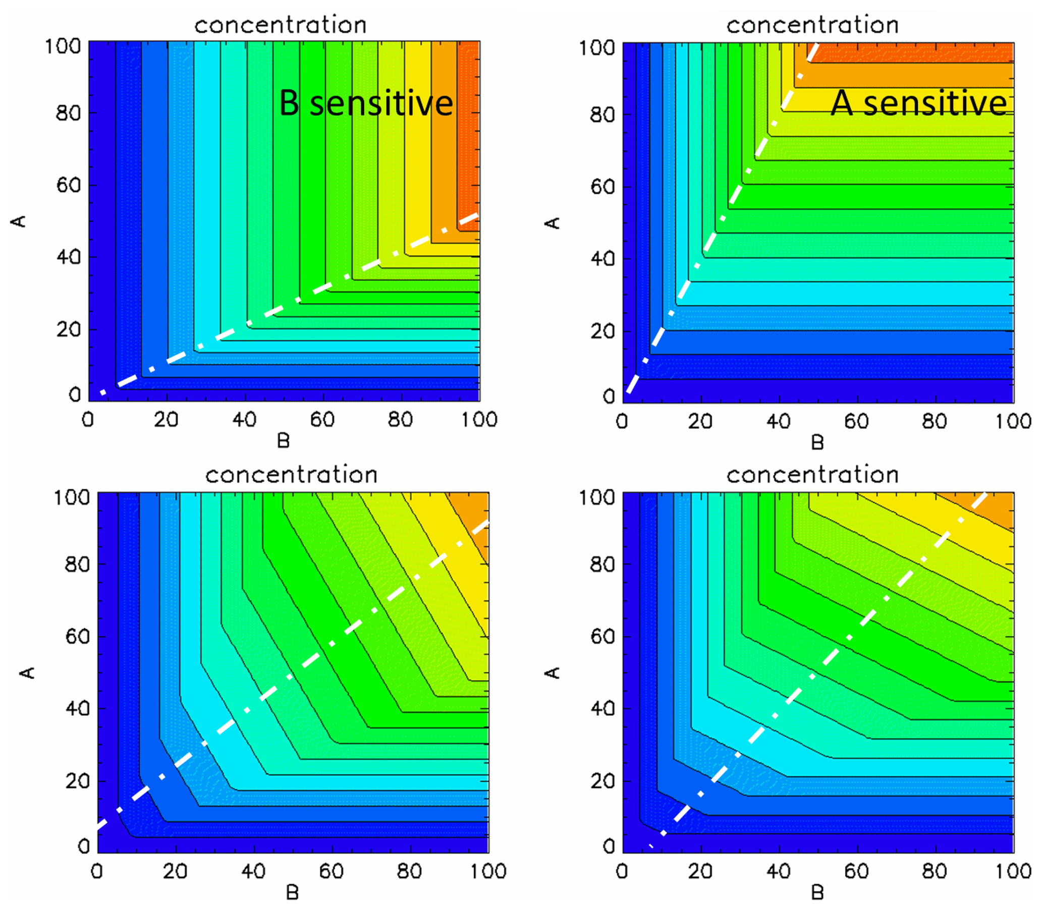
Figure B1Isopleths for a simple theoretical system consisting of two emission precursors (A and B) competing through non-linear reactions to the concentration of a pollutant. See details in the text.
The Open Source EMEP model and all necessary input data to run the model are available through this link: https://github.com/metno/emep-ctm (Norwegian Meteorological Institute, 2021).
Data are in the process of being transferred to a public repository. In the meantime they are available upon request to the authors.
PT and AC designed the methodology, analysed the results and drafted a first version of the paper. MB and JPP contributed to the analysis and interpretation of the results. ADM and JM performed the simulations. CC contributed to the data treatment and visualization aspects. All co-authors critically reviewed the paper.
The authors declare that they have no conflict of interest.
This paper was edited by Astrid Kiendler-Scharr and reviewed by two anonymous referees.
Andersson-Sköld, Y. and Simpson, D.: Comparison of the chemical schemes of the EMEP MSC-W and the IVL photochemical trajectory models, Atmos. Environ., 33, 1111–1129, 1999.
Ansari, A. S. and Pandis, S.: Response of inorganic PM to precursor concentrations, Environ. Sci. Technol., 32, 2706–2714, 1998.
Beekmann, M., Prévôt, A. S. H., Drewnick, F., Sciare, J., Pandis, S. N., Denier van der Gon, H. A. C., Crippa, M., Freutel, F., Poulain, L., Ghersi, V., Rodriguez, E., Beirle, S., Zotter, P., von der Weiden-Reinmüller, S.-L., Bressi, M., Fountoukis, C., Petetin, H., Szidat, S., Schneider, J., Rosso, A., El Haddad, I., Megaritis, A., Zhang, Q. J., Michoud, V., Slowik, J. G., Moukhtar, S., Kolmonen, P., Stohl, A., Eckhardt, S., Borbon, A., Gros, V., Marchand, N., Jaffrezo, J. L., Schwarzenboeck, A., Colomb, A., Wiedensohler, A., Borrmann, S., Lawrence, M., Baklanov, A., and Baltensperger, U.: In situ, satellite measurement and model evidence on the dominant regional contribution to fine particulate matter levels in the Paris megacity, Atmos. Chem. Phys., 15, 9577–9591, https://doi.org/10.5194/acp-15-9577-2015, 2015.
Bergström, R., Denier van der Gon, H. A. C., Prévôt, A. S. H., Yttri, K. E., and Simpson, D.: Modelling of organic aerosols over Europe (2002–2007) using a volatility basis set (VBS) framework: application of different assumptions regarding the formation of secondary organic aerosol, Atmos. Chem. Phys., 12, 8499–8527, https://doi.org/10.5194/acp-12-8499-2012, 2012.
Bessagnet, B., Beauchamp, M., Guerreiro, C., de Leeuw, F., Tsyro, S., Colette, A., Meleux, F., Rouïl, L., Ruyssenaars, P., Sauter, F., Velders, G. J. M., Foltescu, V. L., and van Aardenne, J.: Can further mitigation of ammonia emissions reduce exceedances of particulate matter air quality standards?, Environ. Sci. Policy, 44, 149–163, https://doi.org/10.1016/j.envsci.2014.07.011, 2014.
Binkowski, F. and Shankar, U.: The Regional Particulate Matter Model. 1. Model description and preliminary results, J. Geophys. Res., 100, 26191–26209, 1995.
Blanchard, C. L. and Hidy, G. M.: Effects of Changes in Sulfate, Ammonia,and Nitric Acid on Particulate Nitrate Concentrations in the South-eastern United States, J. Air Waste Manage., 53, 283–290, 2003.
Carnevale, C., Pisoni, E., and Volta, M.: A non-linear analysis to detect the origin of PM10 concentrations in Northern Italy, Sci. Total Environ., 409, 182–191, 2020.
Clappier, A., Thunis, P., Putaud, J. P., Beekmann, M., and De Meij, A.: Analysis of the chemical regimes and non-linearity associated to PM2.5 in Europe, Environment International, accepted, 2021.
de Meij, A., Krol, M., Dentener, F., Vignati, E., Cuvelier, C., and Thunis, P.: The sensitivity of aerosol in Europe to two different emission inventories and temporal distribution of emissions, Atmos. Chem. Phys., 6, 4287–4309, https://doi.org/10.5194/acp-6-4287-2006, 2006.
De Meij, A., Thunis, P., Bessagnet, B., and Cuvelier, C.: The sensitivity of the CHIMERE model to emissions reduction scenarios on air quality in Northern Italy, Atmos. Environ., 43, 1897–1907, 2009.
Dodge, M. C.: Effect of selected parameters on predictions of a photochemical model, US Environmental Protection Agency, EPA-600/3-77/048, Research Triangle Park, NC, USA, 1977.
Donahue, N. M., Robinson, A. L., and Pandis, S. N.: Atmospheric organic particulate matter: From smoke to secondary organic aerosol, Atmos. Environ., 43, 94–106, https://doi.org/10.1016/j.atmosenv.2008.09.055, 2009.
EDGAR: Emission Database for Global Atmospheric research, available at: https://edgar.jrc.ec.europa.eu/ (last access: 25 November 2020), 2020.
EEA: Air quality in Europe — 2020 report, EEA Report No 11/2020, available at: https://www.eea.europa.eu/publications/air-quality-in-europe-2020-report (last access: 4 June 2021), 2020.
EMEP: Transboundary acidification and eutrophication and ground level ozone in Europe: Unified EMEP model description, EMEP/MSC-W Report 1/2003, available at: https://emep.int/publ/reports/2003/emep_report_1_part1_2003.pdf (last access: 1 June 2021), 2003.
EMEP: EMEP/MSC-W Model – User's Guide July 2011, available at: https://wiki.met.no/_media/emep/page1/userguide_062011.pdf (last access: 1 June 2021), 2011.
Fagerli, H., Simpson, D., and Tsyro, S.: Unified EMEP model: Updates. In EMEP Status Report 1/2004, Transboundary acidification, eutrophication and ground level ozone in Europe. Status Report 1/2004, 11–18, The Norwegian Meteorological Institute, Oslo, Norway, 2004.
Feng, T., Li, G., Cao, J., Bei, N., Shen, Z., Zhou, W., Liu, S., Zhang, T., Wang, Y., Huang, R.-J., Tie, X., and Molina, L. T.: Simulations of organic aerosol concentrations during springtime in the Guanzhong Basin, China, Atmos. Chem. Phys., 16, 10045–10061, https://doi.org/10.5194/acp-16-10045-2016, 2016.
Feng, T., Zhao, S., Bei, N., Wu, J., Liu, S., Li, X., Liu, L., Qian, Y., Yang, Q., Wang, Y., Zhou, W., Cao, J., and Li, G.: Secondary organic aerosol enhanced by increasing atmospheric oxidizing capacity in Beijing–Tianjin–Hebei (BTH), China, Atmos. Chem. Phys., 19, 7429–7443, https://doi.org/10.5194/acp-19-7429-2019, 2019.
Fu, X., Wang, S., Xing, J., Zhang, X., Wang, T., and Hao, J.: Increasing Ammonia Concentrations Reduce the Effectiveness of Particle Pollution Control Achieved via SO2 and NOx Emissions Reduction in East China, Environ. Sci. Tech. Let., 4, 221–227, https://doi.org/10.1021/acs.estlett.7b00143, 2017.
Fu, X., Wang, T., Gao, J., Wang, P., Liu, Y., Wang, S., Zhao, B., and Xue, L.: Persistent Heavy Winter Nitrate Pollution Driven by Increased Photochemical Oxidants in Northern China, Environ. Sci. Technol., 54, 3881–3889, https://doi.org/10.1021/acs.est.9b07248, 2020.
Guo, H., Otjes, R., Schlag, P., Kiendler-Scharr, A., Nenes, A., and Weber, R. J.: Effectiveness of ammonia reduction on control of fine particle nitrate, Atmos. Chem. Phys., 18, 12241–12256, https://doi.org/10.5194/acp-18-12241-2018, 2018.
Hakimzadeh, M., Soleimanian, E., Mousavi, A., Borgini, A., De Marco, C., Ruprecht, A., and Sioutas, C.: The impact of biomass burning on the oxidative potential of PM2.5 in the metropolitan area of Milan, Atmos. Environ., 224, 117328, https://doi.org/10.1016/j.atmosenv.2020.117328, 2020.
Huang, L., Wang Q., Wang Y., Emery C., Zhu, A., Zhua, Y., Yin, S., and Yarwood, G., Zhang, K., and Lim, L.: Simulation of secondary organic aerosol over the Yangtze River Delta region: The impacts from the emissions of intermediate volatility organic compounds and the SOA modeling framework, Atmos. Environ., 246, 118079, https://doi.org/10.1016/j.atmosenv.2020.118079, 2020.
Kenagy, H. S., Sparks, T. L., Ebben, C. J., Wooldrige, P. J., Lopez-Hilfiker, F. D., Lee, B. H., Thornton, J. A., McDuffie, E. E., Fibiger, D. L., Brown, S. S., Montzka, D. D., Weinheimer, A. J., Schroder, J. C., Campuzano-Jost, P., Day, D. A., Jimenez, J. L., Dibb, J. E., Campos, T., Shah, V., Jaeglé, L., and Cohen, R. C.: NOx lifetime and NOy partitioning during WINTER, J. Geophys. Res.-Atmos., 123, 9813–9827, https://doi.org/10.1029/2018JD028736, 2018.
Kleinman, L. I.: Seasonal dependence of boundary layer peroxide concentration: The low and high NOx regimes, J. Geophys. Res, 96, 20721–20733, 1991.
Kroll, J. H. and Seinfeld, J. H.: Chemistry of secondary organic aerosol: Formation and evolution of low-volatility organics in the atmosphere, Atmos. Environ., 42, 3593–3624, 2008.
Lachatre, M., Fortems-Cheiney, A., Foret, G., Siour, G., Dufour, G., Clarisse, L., Clerbaux, C., Coheur, P.-F., Van Damme, M., and Beekmann, M.: The unintended consequence of SO2 and NO2 regulations over China: increase of ammonia levels and impact on PM2.5 concentrations, Atmos. Chem. Phys., 19, 6701–6716, https://doi.org/10.5194/acp-19-6701-2019, 2019.
Larsen, B., Gilardoni, S., Stenström, K., Niedzialek, J., Jimenez, J., and Belis, C.: Sources for PM air pollution in the Po Plain, Italy: II. Probabilistic uncertainty characterization and sensitivity analysis of secondary and primary sources, Atmos. Environ., 50, 203–213, https://doi.org/10.1016/j.atmosenv.2011.12.038, 2012.
Le, T., Wang, Y., Liu, L., Yang, J., Yung, Y., Li, G., and Seinfeld, J.: Unexpected air pollution with marked emission reductions during the COVID-19 outbreak in China, Science, 369, eabb7431, doi;10.1126/science.abb7431, 2020.
Leung, D., Shi, H., Zhao, B., Wang, J., Ding, E.M., Gu, Y., Zheng, H., Chen, G., Liou, K. N., Wang, S., Fast, J. D., Zheng, G., Jiang, J., Li, X., and Jiang, J. H.: Wintertime Particulate Matter Decrease Buffered by Unfavorable Chemical Processes Despite Emissions Reductions in China, Geophys. Res. Lett., 47, 14, https://doi.org/10.1029/2020GL087721, 2020.
Li, G., Zavala, M., Lei, W., Tsimpidi, A. P., Karydis, V. A., Pandis, S. N., Canagaratna, M. R., and Molina, L. T.: Simulations of organic aerosol concentrations in Mexico City using the WRF-CHEM model during the MCMA-2006/MILAGRO campaign, Atmos. Chem. Phys., 11, 3789–3809, https://doi.org/10.5194/acp-11-3789-2011, 2011.
Logan, J. A.: An analysis of ozonesonde data for the troposhere: Recommendations for testing 3-D models and development of a gridded climatology for troposheric ozone, J. Geophys. Res., 10, 115–116, 1998.
Makar, P. A., Moran, M. D., Zheng, Q., Cousineau, S., Sassi, M., Duhamel, A., Besner, M., Davignon, D., Crevier, L.-P., and Bouchet, V. S.: Modelling the impacts of ammonia emissions reductions on North American air quality, Atmos. Chem. Phys., 9, 7183–7212, https://doi.org/10.5194/acp-9-7183-2009, 2009.
Nenes, A., Pandis, S. N., Weber, R. J., and Russell, A.: Aerosol pH and liquid water content determine when particulate matter is sensitive to ammonia and nitrate availability, Atmos. Chem. Phys., 20, 3249–3258, https://doi.org/10.5194/acp-20-3249-2020, 2020.
Norwegian Meteorological Institute (Met.no): Open Source EMEP/MSC-W model, available at: https://github.com/metno/emep-ctm, last access: 4 June 2021.
Pay, M. T., Jimenez-Guerrero, P., and Baldasano, J. M.: Assessing sensitivity regimes of secondary inorganic aerosol formation in Europe with the CALIOPE-EU modeling system, Atmos. Environ., 51, 146–164, 2012.
Pernigotti, D., Georgieva, E., Thunis, P., and Bessagnet, B: Impact of meteorological modelling on air quality: Summer and winter episodes in the Po valley (Northern Italy), Int. J. Envir. Poll., 50, 111–119, 2014.
Petetin, H., Sciare, J., Bressi, M., Gros, V., Rosso, A., Sanchez, O., Sarda-Estève, R., Petit, J.-E., and Beekmann, M.: Assessing the ammonium nitrate formation regime in the Paris megacity and its representation in the CHIMERE model, Atmos. Chem. Phys., 16, 10419–10440, https://doi.org/10.5194/acp-16-10419-2016, 2016.
Pinder, R. W., Gilliland, A. B., and Dennis, R. L.: Environmental impact of atmospheric NH3 emissions under present and future conditions in the eastern United States, Geophys. Res. Lett., 35, L12808, https://doi.org/10.1029/2008GL033732, 2008.
Pozzer, A., Tsimpidi, A. P., Karydis, V. A., de Meij, A., and Lelieveld, J.: Impact of agricultural emission reductions on fine-particulate matter and public health, Atmos. Chem. Phys., 17, 12813–12826, https://doi.org/10.5194/acp-17-12813-2017, 2017.
Putaud, J.-P., Pozzoli, L., Pisoni, E., Martins Dos Santos, S., Lagler, F., Lanzani, G., Dal Santo, U., and Colette, A.: Impacts of the COVID-19 lockdown on air pollution at regional and urban background sites in northern Italy, Atmos. Chem. Phys., 21, 7597–7609, https://doi.org/10.5194/acp-21-7597-2021, 2021.
Raffaelli, K., Deserti, M., Stortini, M., Amorati, R., Vasconi, M., and Giovannini, G.: Improving Air Quality in the Po Valley, Italy: Some Results by the LIFE-IP-PREPAIR Project, Atmosphere, 11, 429, https://doi.org/10.3390/atmos11040429, 2020.
Ricciardelli, I., Bacco D., Rinaldi M., Bonafe G., Scotto F., Trentini, A., Bertacci, G., Ugolini, P., Zigola, C., Rovere, F., Maccone, C., Pironi, C., and Poluzzi, V.: A three-year investigation of daily PM2.5 main chemical components in four sites: the routine measurement program of the Supersito Project (Po Valley, Italy), Atmos. Environ., 152, 418e430, https://doi.org/10.1016/J.ATMOSENV.2016.12.052, 2017.
Robinson, A. L., Donahue, N. M., Shrivastava, M. K., Weitkamp, E. A., Sage, A. M., Grieshop, A. P., Lane, T. E., Pierce, J. R., and Pandis, S. N.: Rethinking Organic Aerosols: Semivolatile Emissions and Photochemical Aging, Science, 315, 1259–1262, https://doi.org/10.1126/science.1133061, 2007.
Seinfeld, J. H. and Pandis, S. N.: Atmospheric Chemistry and Physics: From Air Pollution to Global Change, 2nd edn., J. Wiley and Sons, New York, 2006.
Shah, V., Jaeglé, L., Thornton, J. A., Lopez-Hilfiker, F. D., Lee, B. H., Schroder, J. C., Campuzano-Jost, P., Jimenez, J. L., Guo, H., Sullivan, A. P., Weber, R. J., Green, J. R., Fiddler, M. N., Bililign, S., Campos, T. L., Stell, M., Weinheimer, A. J., Montzka, D. D., and Brown, S. S.: Chemical feedbacks weaken the wintertime response of particulate sulfate and nitrate to emissions reductions over the eastern United States, P. Natl. Acad. Sci. USA, 115, 8110–8115, https://doi.org/10.1073/pnas.1803295115, 2018.
Sheng, F., Jingjing, L., Yu., C., Fu-Ming, T., Xuemei, D., and Jing-yao, L.: Theoretical study of the oxidation reactions of sulfurous acid/sulfite with ozone to produce sulfuric acid/sulfate with atmospheric implications, RSC Advances, 8, 7988–7996, https://doi.org/10.1039/C8RA00411K, 2018.
Shrivastava, M., Cappa, C. D., Fan, J., Goldstein, A. H., Guenther, A. B., Jimenez, J. L., Kuang, C., Laskin, A., Martin, S. T., Ng, N. L., Petaja, T., Pierce, J. R., Rasch, P. J., Roldin, P., Seinfeld, J. H., Shilling, J., Smith, J. N., Thornton, J. A., Volkamer, R., Wang, J., Worsnop, D. R., Zaveri, R. A., Zelenyuk, A., and Zhang, Q.: Recent advances in understanding secondary organic aerosol: Implications for global climate forcing, Rev. Geophys., 55, 509–559, https://doi.org/10.1002/2016RG000540, 2017.
Simpson, D., Fagerli, H., Jonson, J. E., Tsyro, S., Wind, P., and Tuovinen, J. P.: The EMEP Unified Eulerian Model. Model Description, EMEP MSC-W Report 1/2003, The Norwegian Meteorological Institute, Oslo, Norway, 2003.
Simpson, D., Benedictow, A., Berge, H., Bergström, R., Emberson, L. D., Fagerli, H., Flechard, C. R., Hayman, G. D., Gauss, M., Jonson, J. E., Jenkin, M. E., Nyíri, A., Richter, C., Semeena, V. S., Tsyro, S., Tuovinen, J.-P., Valdebenito, Á., and Wind, P.: The EMEP MSC-W chemical transport model – technical description, Atmos. Chem. Phys., 12, 7825–7865, https://doi.org/10.5194/acp-12-7825-2012, 2012.
Stein, U. and Alpert, P.: Factor separation in numerical simulations, J. Atmos. Sci., 50, 2107–2115, 1993.
Thunis, P. and Clappier, A.: Indicators to support the dynamic evaluation of air quality models, Atmos. Environ., 98, 402–409, 2014.
Thunis, P., Pernigotti, D., Cuvelier, C., Georgieva, E., Gsella, A., De Meij, A., Pirovano, G., Balzarini, A., Riva, G. M., Carnevale, C., Pisoni, E., Volta, M., Bessagnet, B., Kerschbaumer, A.,Viaene, P., De Ridder, K., Nyiri, A., and Wind, P.: POMI: A Model Intercomparison exercise over the Po valley, Air Qual. Atmos. Hlth, 6, 701–715, https://doi.org/10.1007/s11869-013-0211-1, 2013.
Thunis, P., Clappier, A., Pisoni, E., and Degraeuwe, B.: Quantification of non-linearities as a function of time averaging in regional air quality modeling applications, Atmos. Environ., 103, 263–275, 2015.
Tsigaridis, K., Daskalakis, N., Kanakidou, M., Adams, P. J., Artaxo, P., Bahadur, R., Balkanski, Y., Bauer, S. E., Bellouin, N., Benedetti, A., Bergman, T., Berntsen, T. K., Beukes, J. P., Bian, H., Carslaw, K. S., Chin, M., Curci, G., Diehl, T., Easter, R. C., Ghan, S. J., Gong, S. L., Hodzic, A., Hoyle, C. R., Iversen, T., Jathar, S., Jimenez, J. L., Kaiser, J. W., Kirkevåg, A., Koch, D., Kokkola, H., Lee, Y. H., Lin, G., Liu, X., Luo, G., Ma, X., Mann, G. W., Mihalopoulos, N., Morcrette, J.-J., Müller, J.-F., Myhre, G., Myriokefalitakis, S., Ng, N. L., O'Donnell, D., Penner, J. E., Pozzoli, L., Pringle, K. J., Russell, L. M., Schulz, M., Sciare, J., Seland, Ø., Shindell, D. T., Sillman, S., Skeie, R. B., Spracklen, D., Stavrakou, T., Steenrod, S. D., Takemura, T., Tiitta, P., Tilmes, S., Tost, H., van Noije, T., van Zyl, P. G., von Salzen, K., Yu, F., Wang, Z., Wang, Z., Zaveri, R. A., Zhang, H., Zhang, K., Zhang, Q., and Zhang, X.: The AeroCom evaluation and intercomparison of organic aerosol in global models, Atmos. Chem. Phys., 14, 10845–10895, https://doi.org/10.5194/acp-14-10845-2014, 2014.
Tsimpidi, A. P., Karydis, V. A., Zavala, M., Lei, W., Molina, L., Ulbrich, I. M., Jimenez, J. L., and Pandis, S. N.: Evaluation of the volatility basis-set approach for the simulation of organic aerosol formation in the Mexico City metropolitan area, Atmos. Chem. Phys., 10, 525–546, https://doi.org/10.5194/acp-10-525-2010, 2010.
Tsimpidi, A. P., Karydis, V. A., Pandis, S. N., and Lelieveld, J.: Global combustion sources of organic aerosols: model comparison with 84 AMS factor-analysis data sets, Atmos. Chem. Phys., 16, 8939–8962, https://doi.org/10.5194/acp-16-8939-2016, 2016.
Vahedpour, M., Goodarzi, M., Hajari, N., and Nazari, F.: Struct. Chem., 22, 817—822, 2011.
Watson, J. G., Chow, J. C., Lurmann, F. W., and Musarra, S. P.: Ammonium Nitrate, Nitric Acid, and Ammonia Equilibrium in Wintertime Phoenix, Arizona, Air & Waste, 44, 405–412, https://doi.org/10.1080/1073161X.1994.10467262, 1994.
Womack, C. C., McDuffie, E. E., Edwards, P. M., Bares, R., de Gouw, J. A., Docherty, K. S., Dube, W. P., Fibiger, D. L., Franchin, A., Gilman, J. B., Goldberger, L., Lee, B. H., Lin, J. C., Long, R., Middlebrook, A. M., Millet, D. B., Moravek, A., Murphy, J. G., Quinn, P. K., Riedel, T. P., Roberts, J. M., Thornton, J. A., Valin, L. C., Veres, P. R., Whitehill, A. R., Wild, R. J., Warneke, C., Yuan, B., Baasandorj, M., and Brown, S. S.: An odd oxygen framework for wintertime ammonium nitrate aerosol pollution in urban areas: NOx and VOC control as mitigation strategies, Geophys. Res. Lett., 46, 4971–4979, https://doi.org/10.1029/2019GL082028, 2019.
Xing, J., Ding, D., Wang, S., Zhao, B., Jang, C., Wu, W., Zhang, F., Zhu, Y., and Hao, J.: Quantification of the enhanced effectiveness of NOx control from simultaneous reductions of VOC and NH3 for reducing air pollution in the Beijing–Tianjin–Hebei region, China, Atmos. Chem. Phys., 18, 7799–7814, https://doi.org/10.5194/acp-18-7799-2018, 2018.
- Abstract
- Introduction
- Methodology
- Baseline concentrations of PM2.5 and gaseous inorganic precursors
- Analysis of the SIA formation chemical regimes
- Analysis of non-linearities
- Discussion
- Conclusions
- Appendix A: Selection of seasons
- Appendix B: A theoretical example for the isopleths
- Code availability
- Data availability
- Author contributions
- Competing interests
- Review statement
- References