the Creative Commons Attribution 4.0 License.
the Creative Commons Attribution 4.0 License.
 | 21 Jan 2021
Effective radiative forcing from emissions of reactive gases and aerosols – a multi-model comparison
Gillian D. Thornhill
William J. Collins
Ryan J. Kramer
Dirk Olivié
Ragnhild B. Skeie
Fiona M. O'Connor
Nathan Luke Abraham
Ramiro Checa-Garcia
Susanne E. Bauer
Makoto Deushi
Louisa K. Emmons
Piers M. Forster
Larry W. Horowitz
Ben Johnson
James Keeble
Jean-Francois Lamarque
Martine Michou
Michael J. Mills
Jane P. Mulcahy
Gunnar Myhre
Pierre Nabat
Vaishali Naik
Naga Oshima
Michael Schulz
Christopher J. Smith
Toshihiko Takemura
Simone Tilmes
Tongwen Wu
Guang Zeng
Jie Zhang
This paper quantifies the pre-industrial (1850) to present-day (2014) effective radiative forcing (ERF) of anthropogenic emissions of NOX, volatile organic compounds (VOCs; including CO), SO2, NH3, black carbon, organic carbon, and concentrations of methane, N2O and ozone-depleting halocarbons, using CMIP6 models. Concentration and emission changes of reactive species can cause multiple changes in the composition of radiatively active species: tropospheric ozone, stratospheric ozone, stratospheric water vapour, secondary inorganic and organic aerosol, and methane. Where possible we break down the ERFs from each emitted species into the contributions from the composition changes. The ERFs are calculated for each of the models that participated in the AerChemMIP experiments as part of the CMIP6 project, where the relevant model output was available.
The 1850 to 2014 multi-model mean ERFs (± standard deviations) are −1.03 ± 0.37 W m−2 for SO2 emissions, −0.25 ± 0.09 W m−2 for organic carbon (OC), 0.15 ± 0.17 W m−2 for black carbon (BC) and −0.07 ± 0.01 W m−2 for NH3. For the combined aerosols (in the piClim-aer experiment) it is −1.01 ± 0.25 W m−2. The multi-model means for the reactive well-mixed greenhouse gases (including any effects on ozone and aerosol chemistry) are 0.67 ± 0.17 W m−2 for methane (CH4), 0.26 ± 0.07 W m−2 for nitrous oxide (N2O) and 0.12 ± 0.2 W m−2 for ozone-depleting halocarbons (HC). Emissions of the ozone precursors nitrogen oxides (NOx), volatile organic compounds and both together (O3) lead to ERFs of 0.14 ± 0.13, 0.09 ± 0.14 and 0.20 ± 0.07 W m−2 respectively. The differences in ERFs calculated for the different models reflect differences in the complexity of their aerosol and chemistry schemes, especially in the case of methane where tropospheric chemistry captures increased forcing from ozone production.
- Article
(2198 KB) - Full-text XML
-
Supplement
(1043 KB) - BibTeX
- EndNote


The characterization of the responses of the atmosphere, climate and Earth systems to various forcing agents is essential for understanding, and countering, the impacts of climate change. As part of this effort there have been several projects directed at using climate models from different groups around the world to produce a systematic comparison of the simulations from these models, via the Coupled Model Intercomparison Project (CMIP), which is now in its sixth iteration (Eyring et al., 2016). This CMIP work has been subdivided into different areas of interest for addressing specific questions about climate change, such as the impact of aerosols and reactive greenhouse gases, and the AerChemMIP (Collins et al., 2017) project is designed to examine the specific effects of these factors on the climate. The aerosol and aerosol precursor species considered are sulfur dioxide (SO2), black carbon (BC) and organic carbon (OC). The reactive greenhouse gases and ozone precursors are methane (CH4), nitrogen oxide (NOX), volatile organic compounds (VOCs – including carbon monoxide), nitrous oxide (N2O) and ozone-depleting halocarbons (HC).
The focus of this work is to characterize the effect of the change from pre-industrial (1850) to present day (2014) in aerosols and their precursors, as well as the effect of chemically reactive greenhouse gases (including species that affect ozone) on the radiation budget of the planet, referred to as radiative forcing, as an initial step to understanding the response of the atmosphere and Earth system to changes in these components. In previous reports of the Intergovernmental Panel on Climate Change (IPCC) the effect of the various forcing agents on the radiation balance has been investigated in terms of the radiative forcing (RF), which is a measure of how the radiative fluxes at the top of the atmosphere (TOA) change in response to changes in for example concentrations or emissions of greenhouse gases and aerosols. There have been several definitions of radiative forcing (Forster et al., 2016; Sherwood et al., 2015), which generally considered the instantaneous radiative forcing (IRF), or a combination of the IRF including the adjustment of the stratospheric temperature to the driver, generally termed the stratospheric-temperature-adjusted radiative forcing. More recently (Boucher, 2013; Chung and Soden, 2015) there has been a move towards using the effective radiative forcing (ERF) as the preferred metric, as this includes the rapid adjustments of the atmosphere to the perturbation, e.g. changes in cloud cover or type, water vapour, and tropospheric temperature, which may affect the overall radiative balance of the atmosphere. In this work, ERF is calculated using two atmospheric model simulations, both with the same prescribed sea surface temperatures (SSTs) and sea ice, but with one having the perturbation we are interested in investigating, e.g. a change in emissions or concentrations of aerosols or reactive gases. The difference in the net TOA flux between these two simulations is then defined as the ERF for that perturbation.
Previous efforts to understand the radiative forcing due to aerosols and reactive gases in CMIP simulations have resulted in a wide spread of values from the different climate models, in part due to a lack of suitable model simulations for extracting the ERF from for example a specific change to an aerosol species. The experiments in the AerChemMIP project have been designed to address this in part by defining consistent model set-ups to be used to calculate the ERFs, although the individual models will still have their own aerosol and chemistry modules, with varying levels of complexity and different approaches.
There are complexities in assessing how a particular forcing agent affects the climate system due to the interactions between some of the reactive gases; for example methane and ozone are linked in complex ways, and this increases the problem of understanding the specific contribution of each to the overall ERFs when one of them is perturbed. An attempt to understand some of these interactions is discussed in Sect. 4.2 below.
The experimental set-up and models used are described in Sect. 2, the methods for calculating the ERFs for the aerosol and chemistry experiments are described in Sect. 3, and the results are discussed in Sect. 4. Final conclusions are drawn in Sect. 5.
2.1 Models
This analysis is based on models participating in the Coupled Model Intercomparison Project (CMIP6) (Eyring et al., 2016), which oversees climate modelling efforts from a number of centres with a view to facilitating comparisons of the model results in a systematic framework. The overall CMIP6 project has a number of sub-projects, where those with interests in specific aspects of the climate can design and request specific experiments to be undertaken by the modelling groups. To understand the effects of aerosols and reactive gases on the climate, a set of experiments was devised under the auspices of AerChemMIP (Collins et al., 2017), described in Sect. 2.2.
The anthropogenic emissions of the aerosols, aerosol precursors and ozone precursors (excluding methane) for use in the models are given by Hoesly et al. (2018) and van Marle et al. (2017). Models use their own natural emissions (Eyring et al., 2016). The well-mixed greenhouse gases (WMGHG), CO2, CH4, N2O and halocarbons, are specified as concentrations either at the surface or in the troposphere. Not all of the models include interactive aerosols, tropospheric chemistry and stratospheric chemistry, which is the ideal for the AerChemMIP experiments, but those models which do not include all these processes provide results for a subset of the experiments described in Sect. 2.2.
Table 1Components used in the Earth system models (a detailed table is in the Supplement, Table S1).

The models included in this analysis are summarized below, and in Table 1 with an overview of the model set-up, aerosol scheme and type of chemistry models used included. A more detailed description of each model and the aerosol and chemistry schemes used in each is available in the Supplement, Table S1.
The CNRM-ESM2-1 model (Séférian et al., 2019; Michou et al., 2020) includes an interactive tropospheric aerosol scheme and an interactive gaseous chemistry scheme only above the level of 560 hPa. The sulfate precursors evolve to SO4 using a simple dependence on latitude. The cloud droplet number concentration (CDNC) depends on SO4, organic matter and sea salt concentrations, so the aerosol cloud albedo effect is represented, although other aerosol–cloud interactions are not.
The UKESM1 model (Sellar et al., 2020) includes an interactive stratosphere–troposphere gas-phase chemistry scheme (Archibald et al., 2020) using the UK Chemistry and Aerosol (UKCA; Morgenstern et al., 2009; O'Connor et al., 2014) model. The UKCA aerosol scheme, called GLOMAP mode is two-moment simulation of tropospheric black carbon, organic carbon, SO4 and sea salt. Dust is modelled independently using the bin scheme of Woodward (2001). A full description and evaluation of the chemistry and aerosol schemes in UKESM1 can be found in Archibald et al. (2020) and Mulcahy et al. (2020) respectively.
The MIROC6 model includes the Spectral Radiation-Transport Model for Aerosol Species (SPRINTARS) aerosol model, which predicts mass mixing ratios of the main tropospheric aerosols and models aerosol–cloud interactions in which aerosols alter cloud microphysical properties and affect the radiation budget by acting as cloud condensation and ice nuclei (Takemura et al., 2005, 2018; Watanabe et al., 2010; Takemura and Suzuki, 2019; Tatebe et al., 2019).
The MRI-ESM2 model (Yukimoto et al., 2019) has the Model of Aerosol Species in the Global Atmosphere mark-2 revision-4 climate (MASINGAR mk-2r4c) aerosol model, and a chemistry model, MRI-CCM2 (Deushi and Shibata, 2011), which models chemistry processes for ozone and other trace gases from the surface to middle atmosphere. The model includes aerosol–chemistry interactions and aerosol–cloud interactions (Kawai et al., 2019). The ERFs of anthropogenic gases and aerosols under present-day conditions relative to pre-industrial conditions estimated by MRI-ESM2 as part of the Radiative Forcing Model Intercomparison Project (RFMIP) (Pincus et al., 2016) and AerChemMIP are summarized in Oshima et al. (2020).
The BCC-ESM1 model (Wu et al., 2019, 2020) models major aerosol species including gas-phase chemical reactions and secondary aerosol formation, and aerosol–cloud interactions including indirect effects are represented. It does not include stratospheric chemistry, so concentrations of ozone, CH4 and N2O at the top two model levels are the zonally and monthly values derived from the CMIP6 data package.
The NorESM2 model contains interactive aerosols and uses the OsloAero6 aerosol module (Seland et al., 2020), which describes the formation and evolution of BC, OC, SO4, dust, sea salt and SOA. There is a limited gas-phase chemistry describing the oxidation of the aerosol precursors DMS, SO2, isoprene and monoterpenes; oxidant fields of OH, HO2, NO3 and ozone are prescribed climatological fields; and there is no ozone chemistry in the model.
The GFDL-ESM4 model consists of the GFDL AM4.1 atmosphere component (Dunne et al., 2020; Horowitz et al., 2020), which includes an interactive tropospheric and stratospheric gas-phase and aerosol chemistry scheme. Nitrate aerosols are explicitly treated in this model.
The CESM2-WACCM model includes interactive chemistry and aerosols for the troposphere, stratosphere and lower thermosphere (Emmons et al., 2010); (Gettelman et al., 2019). The representation of secondary organic aerosols follows the volatility basis set approach (Tilmes et al., 2019).
The IPSLCM6A-LR-INCA (referred to subsequently as IPSL-INCA) model used for this analysis has interactive aerosols but a limited gas-phase model. The aerosol scheme is based on a sectional approach to represent the size distribution of dust, sea salt (which has an additional super-coarse mode to model largest emission of spray-salt aerosols), BC, NH4, NO3, SO4, SO2 and organic aerosol (OA) with a combination of accumulation and coarse log-normal modes with both soluble and insoluble treated as independent modes. DMS emissions are prescribed and not interactively calculated. BC is modelled as internally mixed with sulfate (Wang et al., 2016), where the refractive index relies on the Maxwell-Garnett method. Its emissions are derived from inventories. A new dust refractive index is implemented (Di Biagio et al., 2019). Well-mixed trace gas concentrations/emissions are forced with AMIP/CMIP6 datasets (Lurton et al., 2020), ozone using Checa-Garcia et al. (2018) and solar forcing from Matthes et al. (2017).
The GISS-E2-1 model aerosol scheme (one-moment aerosol, OMA) module, which includes sulfate, nitrate, ammonium and carbonaceous aerosols (BC and OC), is coupled to both the tropospheric and stratospheric chemistry scheme. For the results reported here, the physics version 3 of this model configuration was used, which includes the aerosol impacts on clouds. For details of the model, see Bauer et al. (2020).
Table 2List of fixed SST ERF simulations. (“NTCF” as used here excludes methane (Collins et al., 2017). Note that the abbreviation SLCFs (short-lived climate forcers) is used in other publications to refer to near-term climate forcers.)
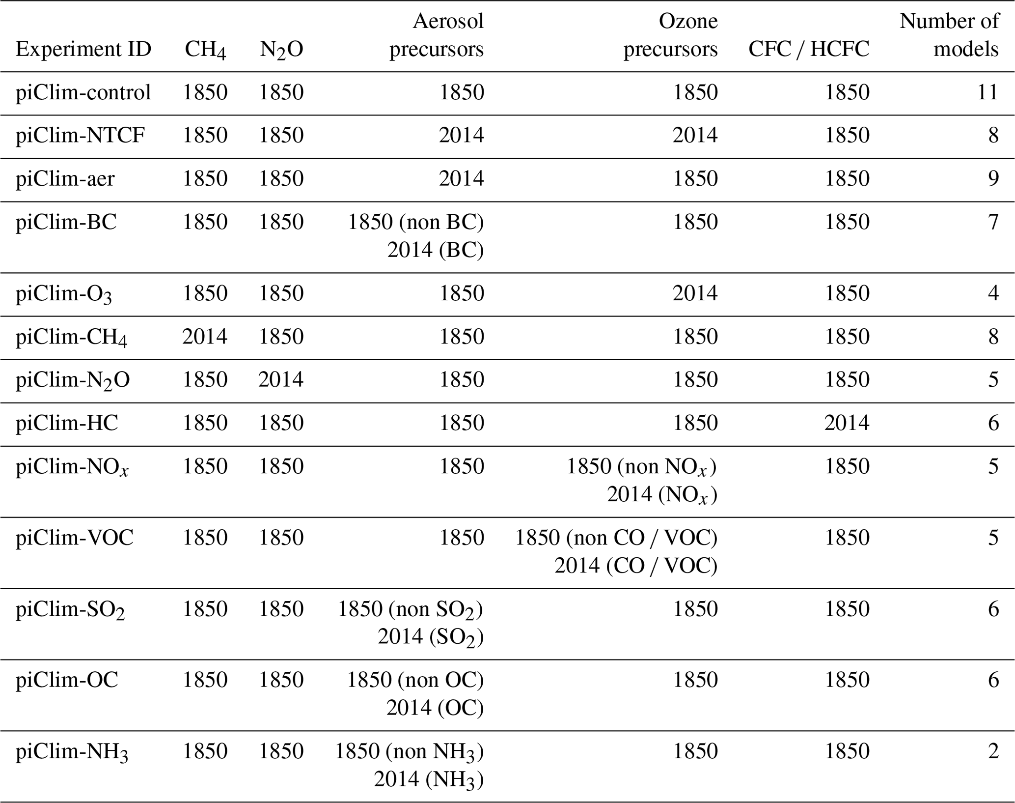
2.2 Experiments
The AerChemMIP time slice experiments (Table 2) are used to determine the present-day (2014) ERFs for the changes in emissions or concentrations of reactive gases, as well as aerosols or their precursors (Collins et al., 2017). The ERFs are calculated by comparing the change in net TOA radiation fluxes between two runs with the same prescribed sea surface temperatures (SSTs) and sea ice, but with near-term climate forcers (NTCFs – also referred to as short-lived climate forcers, SLCFs), reactive gas and aerosol emissions, and well-mixed greenhouse gases (WMGHG – methane, nitrous oxide, halocarbon) concentrations perturbed. It should be noted that in AerChemMIP the NTCF experiment excludes CH4 in the experimental design. The control run uses set 1850 pre-industrial values for the aerosol and aerosol precursors, CH4, N2O, ozone precursors and halocarbons, either as emissions or concentrations (Hoesly et al., 2018; van Marle et al., 2017; Meinshausen et al., 2017). Monthly varying prescribed SSTs and sea ice are taken from the CMIP6 DECK coupled pre-industrial (1850) control simulation. Each experiment then perturbs the pre-industrial value by changing one (or more) of the species (emissions or concentrations) to the 2014 value, while keeping SSTs and sea ice prescribed as in the pre-industrial control. Note that adding individual species to a pre-industrial control will likely give different results to a set-up where species were individually subtracted from a present-day control. The NTCFs are perturbed individually or in groups. This provides ERFs for the specific emission or concentration change but also for all aerosol precursor or NTCFs combined (Collins et al., 2017). For models without interactive tropospheric chemistry “NTCF” and “aer” experiments are the same; in the case of NorESM2 for the NTCF experiments the model attempts to mimic the full chemistry by setting the oxidants and ozone to 2014 values. The WMGHG experiments include the effects on aerosol oxidation, tropospheric and stratospheric ozone, and stratospheric water vapour depending on the model complexity.
Thirty years of simulation are required to minimize internal variability (mainly from clouds) (Forster et al., 2016), and one ensemble member was used for each experiment (almost all models provided only a single ensemble member).
In the following analysis we use several methods to analyse the ERF and the relative contributions from different aerosols, chemistry and processes to the overall ERF for the models and experiments described above, where the appropriate model diagnostics were available.
3.1 Calculation of ERF using fixed SSTs
The ERF is calculated from the experiments described above, where the sea surface temperatures and sea ice are fixed to climatological values. Here the ERF is defined as the difference in the net TOA flux between the perturbed experiments and the piClim-control experiment (Sherwood et al., 2015), calculated as the global mean for the 30 years of the experimental run (where the models were run longer than 30 years, only the last 30 years was used). This allows us to calculate the ERF for the individual species based on the changes to the emission or concentrations between the control and perturbed runs of the models. The assumption is that there is minimal contribution from the climate feedback when the SSTs are fixed, but the resultant ERF includes rapid adjustments to the forcing agent in the atmosphere (Forster et al., 2016).
The ERF calculated using this method includes any contributions to the ERF resulting from changes in the land surface temperature (Ts), which ideally should be removed (Shine et al., 2003; Hansen et al., 2005; Vial et al., 2013) (as the ocean temperature changes are removed by using fixed SSTs). However, there is no simple way to prescribe land surface temperatures in the models considered here analogous to fixing the SSTs, so we make the land surface temperature correction by calculating the surface temperature adjustment from the radiative kernel (see Sect. 3.2) and subtracting it from the standard ERF as calculated above (see also Smith et al., 2020a; Tang et al., 2019). This is designated the ERF_ts to differentiate it from the standard ERF as described above.
3.2 Kernel analysis
Where the relevant data are available, we use the radiative kernel method (Smith et al., 2018; Soden et al., 2008; Chung and Soden, 2015) to break down the ERF into the instantaneous radiative forcing (IRF) and individual rapid adjustments (designated by A), which are radiative responses to changes in atmospheric state variables that are not coupled to surface warming. In this approach, ERF is defined as
where At_trop is the troposphere temperature adjustment, At_strat is the stratosphere temperature adjustment, Ats is the surface temperature adjustment, Aq is the water vapour adjustment, Aa is the albedo adjustment, Ac is the cloud adjustment, and e is the radiative kernel error. Individual rapid adjustments (Ax) are computed as
where is the radiative kernel, a diagnostic tool typically computed with an offline version of a general circulation model (GCM) radiative transfer model that is initialized with climatological base state data, and dx is the climate response of atmospheric state variable x, diagnosed directly from each model. Cloud rapid adjustments (AC) are estimated by diagnosing cloud radiative forcing from model flux diagnostics and correcting for cloud masking using the kernel-derived non-cloud adjustments and IRF, following common practice (e.g. Soden et al., 2008; Smith et al., 2018), whereby
For the calculation of the IRF (for aerosols this is the direct effect) here, the clear-sky IRF (IRFclr) is estimated as the difference between clear-sky ERF (ERFclr) and the sum of kernel-derived clear-sky rapid adjustments (). Since estimates of Ac are dependent on IRF, the same differencing method cannot be used to estimate IRF under all-sky conditions without special diagnostics (in particular the International Satellite Cloud Climatology Project diagnostics (ISCCP) diagnostics) not widely available in the AerChemMIP archive. Instead, for the calculations presented here all-sky IRF is computed by scaling IRFclr by a species-specific factor to account for cloud masking (Soden et al., 2008).
Kernels are available from several sources, and for this analysis we used kernels from CESM (Pendergrass et al., 2018), GFDL (Soden et al., 2008), HadGEM3 (Smith et al., 2020b), and ECHAM6 (Block and Mauritsen, 2013) and took the mean from the four kernels for each model. Overall the individual kernels produced very similar results for each model, as reported in Smith et al. (2018).
3.3 Calculation of ERF using aerosol-free radiative fluxes
To understand the contributions of various processes to the overall ERF we can attempt to separate the ERF that is due to direct radiative forcing from that due to the effects of clouds. Greenhouse gases and aerosols can alter the thermal structure of the atmosphere and hence cloud thermodynamics (the semi-direct effect (Ackerman et al., 2000), and aerosols can act via microphysical effects (e.g. increasing the number of condensation nuclei and decreasing the effective radii of cloud droplets, referred to as the aerosol cloud albedo effect and the cloud lifetime effect (Twomey, 1974; Albrecht, 1989; Pincus and Baker, 1994). Following the method of Ghan (2013) the contribution of the aerosol–radiation interactions to the ERF can be distinguished from that of the aerosol–cloud interactions by using a “double-call” method. This means that the model radiative flux diagnostics are calculated a second time but ignoring the scattering and absorption by the aerosol – referred to in the equations below with “af”. The other effects of the aerosol on the atmosphere (i.e. cloud changes, stability changes, dynamics changes) will still be present, however. The IRFari as defined here is the direct radiative forcing from the aerosol, due to scattering and absorption of radiation. The cloud radiative forcing (ERFaci) due to the aerosol–cloud interactions is then obtained by using the difference between the aerosol-free all-sky fluxes and the aerosol-free clear-sky fluxes, which isolates the cloud effects (see Eqs. 4–6, where Eq. 6 is included for completeness). The ERFaci may include non-cloud rapid adjustments in cloudy regions of the atmosphere. The final term is the ERF as calculated from fluxes with neither clouds nor aerosols (ERFcs, af).
The ERFs are calculated in the same way as for the all-sky ERF described in Sect. 3.1, except that the all-sky radiative flux diagnostics are replaced by the relevant aerosol-free fluxes for both the clear-sky and all-sky cases.
Separating the IRF in Eq. (1) into aerosols and greenhouse gas contributions, IRF = IRFaer + IRFGHG, we can re-write Eqs. (4)–(6).
So ERFaci is equivalent to AC in Eq. (3) with extra terms to account for the all-sky–clear-sky difference in the non-cloud adjustments and all-sky–clear-sky difference in any greenhouse gas IRF. With no greenhouse gas changes ERFcs,af is the total clear-sky non-cloud adjustment. Ghan (2013) attributes this mostly to the surface albedo change ; however, the kernel analysis shows other non-cloud adjustments are larger (Table S4). For greenhouse gases ERFcs,af is the total clear-sky ERF. Assuming the non-cloud adjustments are small apart from Tstrat (Table S4), ERFcs,af is approximately . The is expected to be an overestimate of SARFGHG by 10 %–40 % due to cloud masking (Myhre and Stordal, 1997). Thus for greenhouse gases the ERFaci will be a combination of the cloud adjustment and cloud masking.
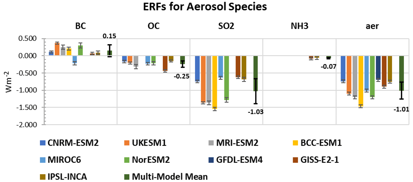
Figure 1Aerosol ERFs for the models with the available diagnostics for the aerosol species experiments, with interannual variability represented by error bars showing the standard error. The piClim-aer experiments include the BC and OC SO2 aerosols, and for GISS-E2-1 and IPSL-INCA NH3 aerosols are also included. The multi-model mean is shown with the mean value and error bars indicating the standard deviation.
4.1 Aerosols and precursors
4.1.1 Inter-model variability
The ERFs are calculated as described in Sect. 3.1, and the summary chart of the ERFs is shown in Fig. 1 for those models with available results – it should be noted that not all models ran all the experiments. The multi-model mean is shown as a separate bar in Fig. 1, with the value given and the standard error indicated with error bars. A table of the individual values for each model and the multi-model mean are included Table S2 in the Supplement.
For the piClim-BC results, the range of values is from −0.21 to 0.37 W m−2, while the MIROC6 model has a negative ERF for BC, contrasting with the positive values from the other models – see further discussion on this in Sect. 4.1.2.
The experiments for the OC (organic carbon) have a range from −0.44 to −0.15 W m−2, and the variability between the models is much less than for the other experiments. The calculated ERFs for the SO2 experiment show a variation from −1.54 to −0.62 W m−2, with CNRM-ESM2-1, MIROC6, IPSL-INCA and GISS-E2-1 at the lower end of the range. These models show a smaller rapid adjustment to clouds which would account for this (see Fig. S1); also note that CNRM-ESM2-1 does not include aerosol effects apart from the cloud albedo effect. The two models with results for the NH3 (GISS-E2-1 and IPSL-INCA) experiment have ERFs of −0.08 and −0.06 W m−2 respectively.
The piClim-aer experiment which uses the 2014 values of aerosol precursors and PI (pre-industrial) values for CH4, N2O and ozone precursors shows a range from −1.47 to −0.7 W m−2 among the models, making it difficult to narrow the range of uncertainty of aerosols from global models. However, the range in the CMIP6 models is consistent with that reported in Bellouin et al. (2019), who suggest a probable range of −1.60 to −0.65 W m−2 for the total aerosol ERF, and compares well with the range of −1.37 to −0.63 W m−2 for the set of piClim-aer experiments considered in Smith et al. (2020a) as part of the RFMIP project. In general, the sum of the ERFs from the individual BC, OC and SO2 experiments does not equal the piClim-aer experiment, due to non-linearity in the aerosol–cloud interactions, particularly since the aerosol perturbation is added to the relatively pristine pre-industrial atmosphere. In the case of GISS, IPSL-INCA and GFDL-ESM4 the models also include nitrate aerosols.
The issue of the effect of perturbing the pre-industrial atmosphere with the aerosol changes is examined in more detail in the Supplement (see Sect. S6) for NorESM2, where a sensitivity analysis was carried out. This analysis does not repeat the AerChemMIP experiments with the perturbation in a present-day atmosphere but examines the effect of adding the SO2 and combined aerosol perturbation to an already polluted present-day atmosphere. In this simplified sensitivity study the differences are 13 % for the SO2 experiment and 20 % for the combined aerosol experiment. However, it should be borne in mind that this is for a specific model, and the perturbed experiment still has the 1850 climate conditions.
The ERF_ts is a simplified method for corrections of land surface warming in fixed sea surface temperature simulations which in addition to land surface changes leads to changes in land surface albedo changes, tropospheric temperature, water vapour and cloud changes (Smith et al., 2020a; Tang et al., 2019).
The ERF_ts values for the models where the land surface temperature adjustment is removed are also included in Supplement Tables S2 and S3 for comparison with the standard ERF. In general, the difference between the two values is small, of the order of 5 %–10 %.

Figure 2Breakdown of the ERFs into the atmospheric rapid adjustments (Atotal) and IRF (instantaneous radiative forcing) for the aerosols. (a) piClim-BC experiment; (b) piClim-SO2 experiment; (c) piClim-OC experiment; (d) piClim-aer experiment.
4.1.2 Breakdown of the ERF into atmospheric adjustments and IRF
The results in Fig. 2 show the ERF as calculated from the radiative fluxes in the fixed SST experiments (Sect. 3.1), the total of the atmospheric adjustments, Atotal, described in Sect. 3.2 (where cf. Eq. 1), and the instantaneous radiative forcing (IRF).
The sum of the IRF and the atmospheric adjustments should equal the overall ERF; however, as the calculation of the IRF depends upon an empirical factor for cloud masking to find the all-sky IRF from the clear-sky IRF (see Sect. 3.2) the sum of the IRF and the Atotal will not necessarily equal the ERF as calculated directly from the model radiative flux diagnostics. However, in general the difference is less than 3 %, suggesting that the approximation used in the calculation of the IRF is reasonable. Using the kernel method described above it is important to note that the IRF calculated here accounts for the presence of the clouds but does not include cloud changes such as the cloud albedo effect.
The models show a variability in the IRF for SO2 (Fig. 2c), with a range of −0.3 to −1.2 W m−2 with the BCC-ESM1 model being the outlier, having the largest overall ERF. The OC experiments (Fig. 2b) range from −0.08 to −0.26 W m−2, with a range for BC of 0.07 to 0.43 W m−2 (Fig. 2a). In MIROC6 the treatment of BC (Takemura and Suzuki, 2019; Suzuki and Takemura, 2019) leads to faster wet removal of BC and hence a lower IRF. For the combined aerosols (Fig. 2d) the range is from −0.1 to −0.6 W m−2.
There are significant differences between the models in the Atotal for SO2; these range from 0.05 to −1.0 W m−2, where the differences are dominated by the cloud adjustments which here include the cloud albedo effect as part of the adjustment (see Fig. S3 for breakdowns of the atmospheric adjustments for all models). The adjustments to BC vary in sign and magnitude, with the MRI-ESM2 and BCC-ESM1 models having a slight positive adjustment. The overall model mean has a weaker negative adjustment to that reported by Stjern et al. (2017), Samset et al. (2016) and Smith et al. (2018). The MIROC6 model has a large negative adjustment which is large enough to lead to an overall negative ERF. We explore the contribution of the individual adjustments to BC in more detail in Fig. 3.
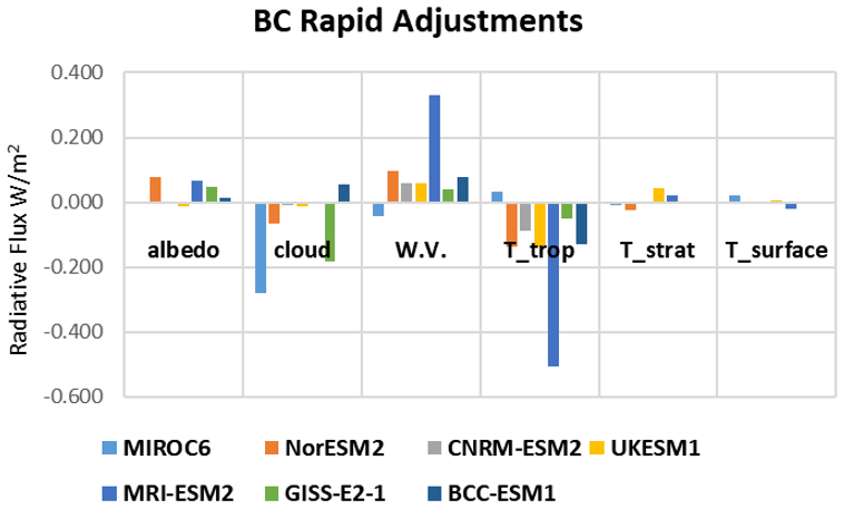
Figure 3Breakdown of the atmospheric adjustments (albedo, cloud, water vapour, troposphere temperature, stratosphere temperature and surface temperature) for the piClim-BC experiments, showing the variability between models.
Examining the breakdown of the rapid adjustments for the piClim-BC experiments (Fig. 3) we see considerable variability in the relative importance of the rapid adjustments; the cloud adjustment dominates in MIROC6, consistent with the increase in low clouds reported for this model, and the treatment of BC as ice nuclei causes the large negative cloud adjustment here (Takemura and Suzuki, 2019; Suzuki and Takemura, 2019). The GISS-E2-1 model also has a strong cloud rapid adjustment, but the larger positive value of the IRF leads to an overall positive ERF for this model. With the exception of MIROC6 the negative tropospheric temperature adjustment is balanced by the water vapour (specific humidity) adjustment, although the magnitude of these adjustments for MRI-ESM2 is at least twice that for the other two models. The interaction of BC with clouds in the MRI-ESM2 model is discussed in detail in Oshima et al. (2020), in particular the impact of BC on ice nucleation in high clouds. The larger surface albedo adjustment for both NorESM2 and MRI-ESM2 is most likely due to the representation of deposition of BC on snow and ice in these models (Oshima et al., 2020).
The piClim-aer experiments (Fig. 1d) show all models have a negative Atotal, covering a range from −0.47 to −1.1 W m−2. Overall, the cloud rapid adjustments dominate for the piClim-aer experiments, with a contribution ranging from −0.45 to −1.1 W m−2 (See Fig. S1). Smith et al. (2020a) also recently diagnosed forcing and adjustments in a similar subset of CMIP6 models for the piClim-aer experiment as part of the Radiative Forcing Model Intercomparison Project (RFMIP) efforts. While they also diagnosed IRF as a residual calculation between ERF and the sum of rapid adjustments, they estimated cloud adjustments using a modified version of the approximate partial radiative perturbation (APRP) method instead of radiative kernels. In their approach, the cloud albedo effect (i.e. Twomey effect) is considered part of the IRF, whereas in the traditional kernel decomposition, it is considered a cloud adjustment. Table S5 compares the two sets of estimates, highlighting the IRF and total cloud adjustment exhibit a near-equal absolute difference between the two studies, and the sum of IRF and total cloud adjustment is in close agreement (mean % difference ∼ 1.0 % for this subset of models). This indicates the classification of the first indirect effect is the only noticeable difference between the two approaches.
The breakdown of the rapid adjustments for all the models is included in Fig. S1, showing the contributions from each type of rapid adjustment for all the experiments for which we have the relevant diagnostics.
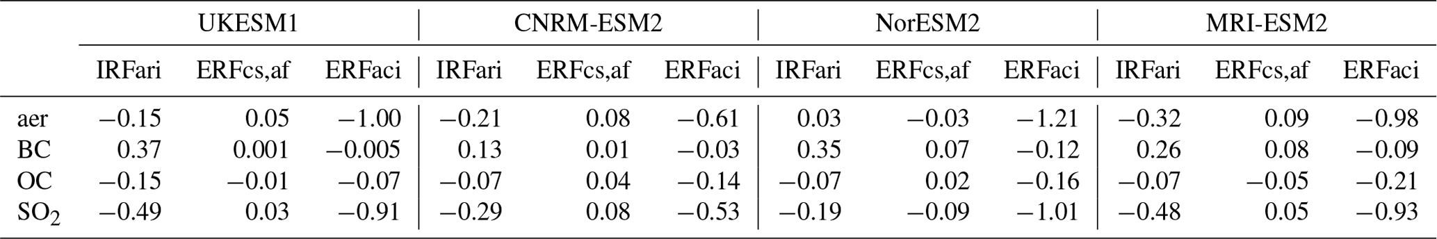
Table 3Results for IRFari, ERFaci and ERFcs,af for aerosol experiments from several models.
4.1.3 Radiation and cloud interactions
The second method of breaking down the ERF to constituents is described in Sect. 3.3 (the Ghan method), the results from which are shown in Table 3. The detailed ERF results for MRI-ESM2 are summarized in Oshima et al. (2020) and for UKESM1 in O'Connor et al. (2020a). Only four of the models under consideration have so far produced the necessary diagnostics for this calculation, and the results are presented in Table 3. For the experiments on aerosols (aer, BC, SO2, OC) the ERFcs,af (non-cloud adjustments) contribution is small, and the ERF is largely a combination of the direct radiative effect, IRFari, and the cloud radiative effect, ERFaci. The IRFari is the direct effect of the aerosol due to scattering and absorption, while the ERFaci is the contribution from the aerosol–cloud interactions and is approximately equal to the rapid adjustments due to clouds (Ac see Sect. 3.2).
For the BC experiment the contribution of the aerosol–cloud interaction has a strong contribution to the overall ERF, except in the case of UKESM1 where it is much weaker; this may be due to the strong short-wave (SW) and long-wave (LW) cloud adjustments in this model cancelling out (O'Connor et al., 2020a; Johnson et al., 2019). The SO2 experiment shows a large cloud radiative effect; in fact the ERFaci is mostly double the IRFari in all the models, due to the large effect on clouds of SO2 and sulfates through the indirect effects. For the OC experiments the ERFaci to IRFari comparison is mixed, with the ERFaci general half or less the IRFari, except in the case of UKESM1, where this ratio is reversed.
The IRFari values are compared with the IRF calculated via the kernel analysis (Sect. 3.2) where the relevant model results are available. These are shown in Fig. S2a; the agreement is generally good, giving confidence in the kernel analysis. Similarly, ERFaci compares well with the cloud adjustment Ac (Fig. S2b).
4.1.4 AOD forcing efficiencies
In order to break down the contributions of the constituent aerosol species to the overall aerosol ERF, we use the AOD (aerosol optical depth) as a forcing efficiency metric for each of the species and use this to assess their contributions to the overall ERF. Not all models had diagnostics available for the AOD for the individual species, so the analysis uses a subset of the models.
Table 4Values of ERF, ΔAOD and ERF ∕ AOD for aerosol experiments for CNRM-ESM2-, MIROC6, Nor-ESM2, GISS-E2-1 and MRI-ESM2 models.
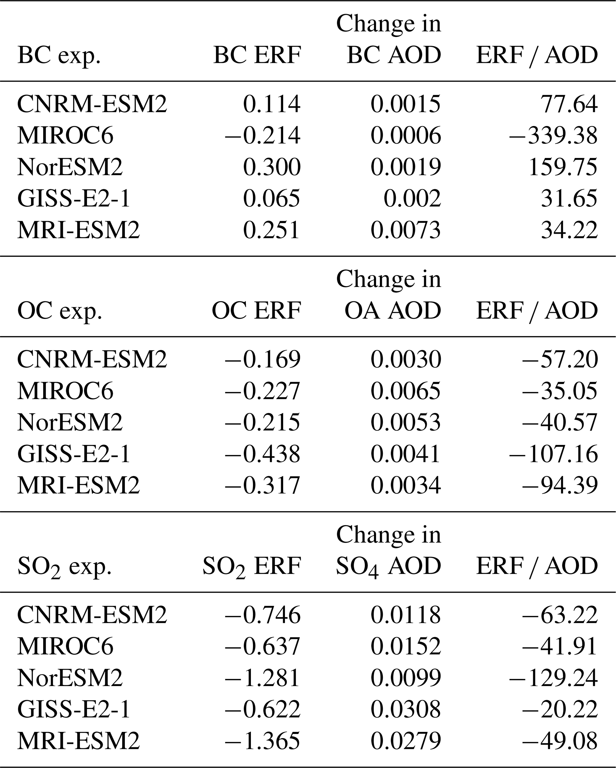
By looking at the single species piClim-BC, piClim-OC and piClim-SO2 experiments, we can find the change in the AOD for the individual species (e.g. ΔAOD for BC for the piClim-BC experiment) and use this to scale the piClim-BC ERF using the AOD change. This assumes that the ERF in the single-species experiment is wholly due to the change in that species as indicated by the AOD, an assumption which is explored in the Supplement in Sect. S4. Table 4 shows the AOD forcing efficiency for the piClim-BC, piClim-SO2 and piClim-OC experiments for each of the five models which had the relevant optical depth diagnostics available.

Figure 4The contributions to the ERF for piClim-aer from the individual species, the sum of the scaled ERFs and the ERF calculated directly from the piClim-aer experiment for five of the models.
The MIROC6 model results in a negative scaling for BC due to the negative ERF for this experiment for this model (Takemura and Suzuki, 2019; Suzuki and Takemura, 2019) (see Sect. 4.1.1). The change in the BC AOD is similar for CNRM-ESM2-1 and Nor-ESM2, and the scale factors reflect the differences in the ERF. The scaling for the SO4 in the NorESM2 experiment is twice that of the other models, suggesting a larger impact of the SO4 AOD on the ERF in this model. These values differ somewhat from those found in Myhre et al. (2013b), where they examined the radiative forcing normalized to the AOD using models in the AeroCom phase II experiments. They found values for sulfate ranging from −8 to −21 W m−2 per unit AOD, which is much weaker than those in our results. However, it is important to note that in the AeroCom phase II experiments the cloud and cloud optical properties are identical between their control and perturbed runs, so no aerosol indirect effects are included, nor are any rapid adjustments (IRFari in Eq. 4). For the BC experiment their values range from 84 to 216 W m−2 per unit AOD, broadly similar to the results presented here (with the exception of the negative MIROC6 result). Their results for OA (organic aerosols) which include fossil fuel and biofuel emissions have values ranging from −10 to −26 W m−2 per unit AOD – weaker than our values for the piClim-OC experiments, which range from −35 to −107 W m−2 per unit AOD but include the cloud indirect effects here.
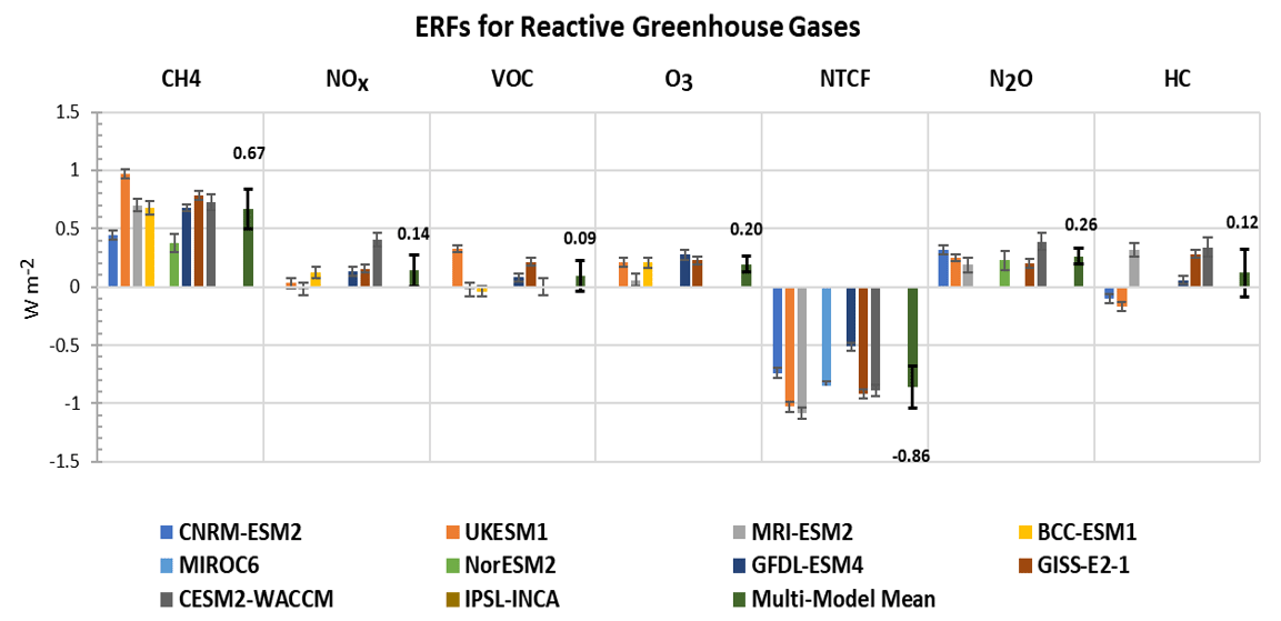
Figure 5Reactive gas ERFs for the models with the available diagnostics for the reactive gas experiments with interannual variability represented by error bars showing the standard error. The multi-model mean is shown with the mean value and error bars indicating the standard deviation.
The sum of the individual AODs from BC, SO4, OA, dust and sea salt gives the total aerosol AOD in the piClim-aer experiment, where the various aerosols were combined. We can then use the AOD for each aerosol in the piClim-aer experiment and the forcing efficiency above to find the contribution of the individual aerosol to the overall change in ERF, providing an approximate estimate of the relative contribution of each aerosol to the overall ERF. In Fig. 4 the relative contributions to the ERF from black carbon (BC), organic aerosols (OA) and sulfate (SO4) are shown for three of the models. The sum of the ERFs from the individual species is also compared to the ERF calculated from the piClim-aer experiment (NB the sea salt and dust contributions to the ERF are less than 1 %, and they are not shown in this figure for clarity – the ERF ∕ AOD forcing efficiency for these is presented in Thornhill et al. (2020). There is considerable variation in the ERF for the piClim-aer experiments between models (see Sect. 4.1), but from this analysis the SO4 is the largest contributor in all cases, although in the case of the MIROC6 model its relative importance is reduced. The positive ERF contribution from the BC tends to partly offset the negative ERF from the OA and SO4, except in the MIROC6 model, where the BC has a negative contribution to the ERF.
The difference between the calculated ERF from the sum of the scaled ERFs is a result of the non-linearity of the aerosol–cloud interactions, a factor which is increased because the aerosols are added to the pre-industrial atmosphere. However, using the IRFari instead of the total ERF to calculate the forcing efficiency and using the same method also results in a difference between the total IRFari derived from the scaled individual experiments and the IRFari for the combined aerosol experiment, suggesting that the difference is not simply a result of the aerosol–cloud interactions.
Using the burden as a scaling factor following the same analysis as described for the AOD results in a largely similar result for the scaling factor, although interestingly the burden scaling for SO2 in the Nor-ESM2 model is similar to the other models (see Table S6 for the burden forcing efficiency).
4.2 Reactive greenhouse gases
The different Earth system models include different degrees of complexity in their chemistry, so their responses to changes in reactive gas concentrations or emissions differ. NorESM2 has no atmospheric chemistry, so there is no change to ozone (tropospheric or stratosphere) or to aerosol oxidation following changes in methane or N2O concentrations. CNRM-ESM2-1 includes stratospheric ozone chemistry but no non-methane hydrocarbon chemistry, and thus ozone is prescribed below 560 hPa. There are no effects of chemistry on aerosol oxidation. BCC-ESM1 includes tropospheric chemistry but not stratospheric chemistry. Stratospheric concentrations are relaxed towards climatological values. UKESM1, GFDL-ESM4, CESM2-WACCM, GISS-E2 and MRI-ESM2 all include tropospheric and stratospheric ozone chemistry as well as changes to aerosol oxidation rates. The ERFs calculated for the reactive gases for several models are shown in Fig. 5, with the multi-model means given in Table S3.
The contributions from gas-phase and aerosol changes to the ERF can be pulled apart to some extent by using the clear-sky and aerosol-free radiation diagnostics (Table 5). The direct aerosol forcing (IRFari) is diagnosed as for the aerosol experiments (Sect. 3.3). The diagnosed changes in aerosol mass are shown in Table S8. GFDL-ESM4 and GISS-ES-1 include nitrate aerosol and show expected responses from NOX emissions (including O3 experiment). CESM2-WACCM shows an increase in secondary organic aerosol from VOC emissions. Sulfate responses are generally inconsistent across the models. There seems little correlation between aerosol mass changes and diagnosed IRFari.
Table 5Calculations of IRFari, ERFaci (cloud) and ERFcs,af for the chemically reactive species.
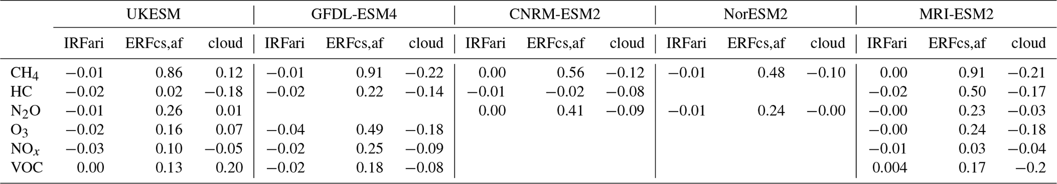
For gas-phase experiments the diagnosed cloud interactions (ERFaf–ERFcs,af) comprise the ERFaci from effects on aerosol chemistry (as in Sect. 3.3) but also any cloud adjustments and effects of cloud masking on the gas-phase forcing (Eq. 8). The clear-sky aerosol-free diagnostic (ERFcs,af) is an indication of the greenhouse gas forcing; however, this will be an overestimate as it neglects cloud masking effects (Sect. 3.3).
4.2.1 ERF vs. SARF
For the reactive greenhouse gases the kernel analysis is used to break down the ERF into the stratospherically adjusted radiative forcing (SARF), which is calculated using the IRF from the kernel analysis (Sect. 3.2), the stratospheric temperature adjustment (At_strat) (SARF = IRF + At_strat), and the tropospheric adjustments (Atrop), which is the sum of the tropospheric atmospheric adjustments. These quantities are plotted in Fig. 6.
For methane the ERFs are largest for those models that include tropospheric ozone chemistry reflecting the increased forcing from ozone production (see Sect. 4.2.2). The analytic calculation for CH4 only based on Etminan et al. (2016) gives a SARF of 0.56 W m−2. The tropospheric adjustments are negative for all models except UKESM1 (Fig. 6). The negative cloud adjustment comes from an increase in the LW emissions, possibly due to less high cloud. In UKESM1 O'Connor et al. (2020b) show that methane decreases sulfate new particle formation, thus reducing cloud albedo and hence a positive cloud adjustment in that model.

Figure 6Breakdown of the ERF into SARF (IRF + At_strat) and tropospheric rapid adjustments (Atrop) for the chemically reactive species (a) for piClim-CH4 experiments, (b) for piClim-HC experiments, (c) for piClim-N2O experiments, (d) for piClim-NOx experiments, (e) for piClim-O3 experiments and (f) for piClim-VOC experiments.
For N2O, results are available for models CNRM-ESM2, NorESM2, MRI-ESM2 and GISS-E2 (the analytic N2O-only calculation gives a SARF of 0.17 W m−2). There appears to be little net rapid adjustment to N2O apart from CESM2-WACCM. Note that due to the method of calculating the all-sky IRF (Sect. 3.2), the IRF and the adjustment terms do not sum to give the ERF.
The models respond very differently to changes in halocarbons. The expected halocarbon-only SARF is +0.30 W m−2 depending on exact speciation used in the model (WMO, 2018). For CNRM-ESM2, UKESM1 and GFDL-ESM4, the ERFs are negative or only slightly positive (see also Morgenstern et al., 2020), whereas for GISSE21 and MRI-ESM2 the ERFs and SARF are both strongly positive. The differences in stratospheric ozone destruction in these models can partially explain the inter-model differences (Sect. 4.2.2).
4.2.2 Ozone changes
The ozone radiative forcing is diagnosed using a kernel to scale the 3D ozone changes based on Skeie et al. (2020). This kernel includes stratospheric temperature adjustment, but not tropospheric adjustments and thus gives a SARF. These are shown in Fig. 7. Corresponding changes in the tropospheric and stratospheric ozone columns are shown in Fig. S5, Increased CH4 concentrations give a SARF for ozone produced by methane of 0.14 ± 0.03 W m−2, and anthropogenic NOx emissions and VOC (including CO) emissions give SARFs of 0.20 ± 0.07 and 0.11 ± 0.04 W m−2 respectively. The O3 experiment comprised both NOx and VOC emission changes. The SARF in this experiment (0.31 ± 0.05 W m−2) is close to the sum of the NOx and VOC experiments (0.30 ± 0.05 W m−2 for the same set of models) showing little non-linearity in the chemistry (Stevenson et al., 2013).
There is a larger variation across models in the stratospheric ozone depletion from halocarbons ( W m−2), with UKESM1 having noticeably larger depletion as seen in Keeble et al. (2020), giving a SARF of −0.33 W m−2. N2O causes some stratospheric ozone depletion in these models, mainly in the tropical upper stratosphere where depletion causes a positive forcing (Skeie et al., 2020), and increases tropospheric ozone (Fig. S6), giving a small net positive SARF (0.03±0.01 W m−2).
Methane oxidation also leads to water vapour production. Figure S6 shows increases in the stratosphere for the piClim-CH4 of up to 20 % . The kernel analysis however finds very low radiative forcing associated with this increase ( W m−2).
4.2.3 Comparison with greenhouse gas forcings
The ERFs, ERFcs,af and SARFs diagnosed for the greenhouse gas changes (Fig. 6, Table 5) are compared with the expected greenhouse gas SARFs in Fig. 8. The expected SARFs from the well-mixed gases are given by Etminan et al. (2016) for CH4 and N2O and by WMO (2018) for the halocarbons (the halocarbon changes are slightly different in each model). The expected SARFs from ozone changes are from Fig. 7.
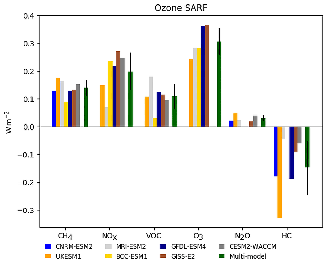
Figure 7Changes in ozone stratospheric-temperature-adjusted radiative forcing (SARF) for each experiment, diagnosed using kernels (see text). Uncertainties for the multi-model means are standard deviations across models.
For methane the ERFs are typically higher than the expected GHG SARF (except for CNRM-ESM2). The diagnosed ERFcs,af and SARF agree better with the expected SARF in UKESM1, BCC-ESM1 and CESM2-WACCM but not in other models. For N2O the modelled ERF is larger than the expected SARF for CNRM-ESM2-1 and CESM2-WACCM; this is explained by the rapid adjustments for CESM2-WACCM but not for CNRM-ESM2. For halocarbons the stratospheric ozone depletion offsets the direct SARF and accounts for much of the spread in the model SARF, although the CNRM-ESM2-1 ERF and SARF are lower than expected. The modelled HC ERF for UKESM1 is strongly negative due to increased aerosol–cloud interactions (O'Connor et al., 2020a; Morgenstern et al., 2020), but removing cloud effects using the SARF or ERFcs,af agrees better with the expected value. The estimated ozone SARF from the NOX, VOC and O3 experiments generally agrees with the model SARF and ERFcs,af. For CESM2-WACCM the ERF from the VOC experiment is zero, and the SARF is negative even though the diagnosed ozone SARF is positive. For all experiments and models ERFcs,af is generally higher than the expected or diagnosed SARF (see Sect. 3.3).

Figure 8Estimated SARF from the greenhouse gas changes (WMGHGs and ozone), using radiative efficiencies for the WMGHGs and kernel calculations for ozone (see text). Hatched bars show decreases in ozone SARF. Symbols show the modelled ERF, SARF and ERFcs,af (estimate of greenhouse gas clear-sky ERF). Uncertainties on the bars are due to uncertainties in radiative efficiencies. Uncertainties on the symbols are errors in the mean due to interannual variability in the model diagnostic.
4.2.4 Methane lifetime
In the CMIP6 set-up the modelled methane concentrations do not respond to changes in oxidation rates. The methane lifetime is diagnosed (which includes stratospheric loss to OH as parameterized within each model), and, assuming losses to chlorine oxidation and soil uptake of 11 and 30 Tg yr−1 (Saunois et al., 2020; Myhre et al., 2013b), this can be used to infer the methane changes that would be expected if methane were allowed to vary. Figure 9 shows the methane lifetime response is large and negative for NOx emissions, with a smaller positive change for VOC emissions. Halocarbon concentration increases decrease the methane lifetime, as ozone depletions lead to increased UV in the troposphere and increased methane loss to chlorine in the stratosphere (Stevenson et al., 2020). N2O also decreases the methane lifetime by depleting ozone in the tropics, although the effect is less than for halocarbons. The O3 experiment has a significantly more negative effect ( %) than the sum of NOx and VOC ( %) (uncertainties are multi-model standard deviation). This suggests significant non-additivity. Note that a combined CH4 + NOx + VOC experiment is not available to test the additivity further.
The lifetime response to changing methane concentrations can be used to diagnose the methane lifetime feedback factor f (Fiore et al., 2009). The results here give f=1.32, 1.31, 1.43, 1.30, 1.26 and 1.19 (mean 1.30±0.07) for UKESM1, MRI-ESM2, BCC-ESM1, GFDL-ESM4, GISS-E2-1 and CESM-WACCM. This is in very good agreement with AR5, although their values are starting from a year 2000 baseline rather than a pre-industrial baseline.
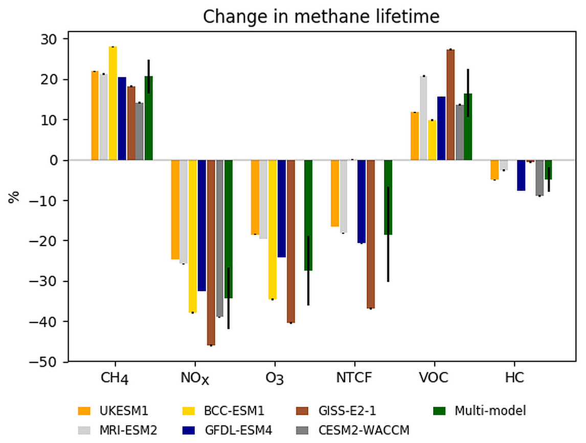
Figure 9Changes in methane lifetime (%), for each experiment. Uncertainties for individual models are errors on the mean from interannual variability. Uncertainties for the multi-model mean are standard deviations across models.
4.2.5 Total ERFs
The methane lifetime changes can be converted to expected changes in concentration if methane were allowed to freely evolve following Fiore et al. (2009), using the f factors appropriate to each model (Sect. 3.3.4). The inferred radiative forcing is based on radiative efficiency of methane (Etminan et al., 2016). The methane changes also have implications for ozone production, so we assume an ozone SARF per parts per billion of CH4 diagnosed for each model from Sect. 4.2.
The breakdown of the information from the analyses above is shown in Fig. 10, using the SARF calculated for the gases (WMGHGs and ozone) and kernel-diagnosed cloud adjustments (which include aerosol–cloud interactions). Direct contributions from the aerosols IRFari are shown for models where this is available. The contributions from methane lifetime changes have also been added to the diagnosed ERF as these are not accounted for in the models. Differences between the diagnosed ERF (stars) and the sum of the components (crosses) then show to what extent this decomposition into components can account for the modelled ERF. For many of the species, this breakdown is reasonable and illustrates that cloud radiative effects can make significant contributions to the total radiative impacts of WMGHGs and ozone precursors. This analysis cannot distinguish between cloud effects due to changes in atmospheric temperature profiles or those due to increased cloud nucleation from aerosols.
For all of the species shown we see considerable variation in the calculated ERFs across the models, which is due in part to differences in the model aerosol and chemistry schemes; not all models have interactive schemes for all of the species, and whether or not chemistry is considered will impact the evolution of some of the aerosol species. We can use the differences in model complexity from the multi-model approach together with the separation of the effects of the various species in the individual AerChemMIP experiments to understand how the various components contribute to the overall ERFs we have calculated.

Figure 10SARF for WMGHGs, ozone and diagnosed changes in methane. Model-diagnosed direct aerosol RF and cloud radiative effect. Crosses mark the sum of the five terms for each model. Stars mark the diagnosed ERF with the effect of methane lifetime (on methane and ozone) added. Differences between stars and crosses show undiagnosed contributions. Uncertainties on the sum are mainly due to the uncertainties in the radiative efficiencies. Uncertainties in the ERF are errors on the mean due to interannual variability. Note that for CESM2-WACCM, BCC-ESM1 and GISSE21 the direct aerosol effect is unavailable.
5.1 Aerosols
The 1850–2014 multi-model mean and standard deviation of the ERFs for SO2, OC and BC are W m−2 for SO2, W m−2 for OC and 0.15 ± 0.17 W m−2 for BC. The total ERF for the aerosols is W m−2, within the range of −1.65 to −0.6 W m−2 reported by Bellouin et al. (2019).
The radiative kernels and double-call diagnostics are used to separate the direct and cloud effects of aerosols for those models where all the relevant diagnostics are available. These two methods broadly agree on the cloud contribution for the BC, SO2 and OC experiments. We generally find a weaker total adjustment to black carbon compared to other studies (Samset and Myhre, 2015; Stjern et al., 2017; Smith et al., 2018). The exceptions are MIROC6 and GISS-E2-1. These previous studies used much larger changes in black carbon (up to 10 times), which may cause non-linear effects such as self-lofting.
As the ISCCP cloud diagnostics become available for more of the CMIP6 models, it will be possible to do a direct calculation of the cloud rapid adjustments using the kernels from Zelinka et al. (2014) and compare those with the adjustments calculated using the kernel difference method described in Smith et al. (2018) and used here (Sect. 3.2; see also Fig. 4 and S2 from Smith et al., 2020a).
The radiative efficiencies per AOD calculated here are generally larger than those from the AeroCom phase II experiments (Myhre et al., 2013b), with the caveat that the models included here did not have fixed clouds, so that indirect effects would be included.
The values diagnosed for the IRFari (for the models we have available diagnostics for) in CMIP6 are similar to those from CMIP5 (Myhre et al., 2013a), where they reported values for sulfate of −0.4 (−0.6 to −0.2) W m−2 compared to our −0.36 (−0.19 to −0.49) W m−2 for the SO2 experiment, they found −0.09 (−0.16 to −0.03) W m−2 compared to our value of −0.09 (−0.07 to −0.15) W m−2 for OC, and they had +0.4 (+0.05 to +0.80) compared to our value of 0.28 (0.13–0.37) W m−2 for BC, so broadly the IRFari values for the individual species agree with those found in the previous set of models used in CMIP5.
The overall aerosol ERF from AR5 is reported as in the range −1.5 to 0.4 W m−2, compared to ERF values reported here for the piClim-aer experiment in the range −0.7 to −1.47 W m−2.
5.2 Reactive greenhouse gases
The diagnosed ERFs from methane, N2O, halocarbons and ozone precursors are 0.75 ± 0.10, 0.26 ± 0.07, 0.12 ± 0.21 and 0.20 ± 0.07 W m−2 (excluding CNRM-ESM2-1 for methane as it cannot represent the lower tropospheric ozone changes and excluding NorESM2 for all as it has no ozone chemistry). These compare with 0.79 ± 0.13, 0.17 ± 0.03, 0.18 ± 0.15 and 0.22 ± 0.14 W m−2 for 1750–2011 from AR5 (Myhre et al., 2013a) – where the effects on methane lifetime and CO2 have been removed from the AR5 calculations, and the halocarbons are for CFCs and HCFCs only. Section 4.2.5 shows that cloud effects can make a significant contribution to the overall ERF even for WMGHGs. However, clouds cannot explain all the differences. The ERF for N2O is larger than estimated in AR5. The ozone contribution here is estimated as 0.03±0.01 W m−2, whereas it was zero in AR5, but that does not explain all the difference. The multi-model ERF for halocarbons is smaller than AR5, due to larger ozone depletion although the models have a wide spread with some showing significantly lower ERFs and some significantly higher due to varying strengths of ozone depletion in these models.
The estimated ozone SARFs from the changes in levels of methane, NOx and VOC from 1850 to 2014 are 0.14±0.03, 0.20±0.07 and 0.11±0.04 W m−2 compared to 0.24±0.13, 0.14±0.09 and 0.11±0.05 W m−2 in CMIP5 (Myhre et al., 2013a). The ozone from methane contribution is smaller, here only 25 % of the direct Etminan et al. (2016) methane SARF compared to 50 % in AR5 (or 39 % using the Etminan et al., 2016, formula). The NOx contribution is larger in this study. The CMIP5 results were based on Stevenson et al. (2013), in which species were reduced from present-day levels rather than being increased from pre-industrial levels. The NOx emission changes are also larger for CMIP6 compared to CMIP5 (Hoesly et al., 2018). The sum of the ozone terms (CH4 + N2O + HC + O3) is 0.33±0.11 W m−2, agreeing well with the total 1850–2014 ozone SARF of 0.35 ± 0.16 W m−2 (1 SD) from Skeie et al. (2020), which included a few additional models.
The overall effect of NTCF emissions (excluding methane and other WMGHGs) on the 1850–2014 ERF experienced by models that include tropospheric chemistry is strongly negative ( W m−2) due to the dominance of the aerosol forcing over that from ozone. There is a large spread in the NTCF forcing due to the different treatment of atmospheric chemistry within these models. Models without tropospheric and/or stratospheric chemistry prescribe varying ozone levels which are not included in the NTCF experiment. Hence the overall forcing experienced by these models due to ozone and aerosols will be different from that diagnosed here.
The experimental set-up and diagnostics in CMIP6 have allowed us for the first time to calculate the effective radiative forcing (ERF) for present-day reactive gas and aerosol concentrations and emissions in a range of Earth system models. Quantifying the forcing in these models is an essential step to understanding their climate responses.
This analysis also allows us to quantify the radiative responses to perturbations in individual species or groups of species. These responses include physical adjustments to the imposed forcing as well as chemical adjustments and adjustments related to the emissions of natural aerosols. The total adjustment is therefore a complex combination of individual process, but the diagnosed ERF implicitly includes these and represents the overall forcing experienced by the models.
We find that the ERF from well-mixed greenhouse gases (methane, nitrous oxide and halocarbons) has significant contributions through their effects on ozone, aerosols and clouds, which vary strongly across Earth system models. This indicates that Earth system processes need to be taken into account when understanding the contribution WMGHGs have made to present climate and when projecting the climate effects of different WMGHG scenarios.
All data from the various Earth system models used in this paper are available on the Earth System Grid Federation website and can be downloaded from there (https://esgf-index1.ceda.ac.uk/search/cmip6-ceda/, ESGF, 2020).
The supplement related to this article is available online at: https://doi.org/10.5194/acp-21-853-2021-supplement.
Manuscript preparation was done by GDT, WJC, RJK and DO with additional contributions from all co-authors. Model simulations were set up, reviewed and/or ran by RChG, DO, FMO'C, NLA, MD, LE, LH, J-FL, MMichou, MMills, JM, PN, VN, NO, MS, TT, ST, TW, GZ and JZ. Analysis was carried out by GT, WC, RK, DO and RS.
The authors declare that they have no conflict of interest.
We acknowledge the World Climate Research Programme, which, through its Working Group on Coupled Modelling, coordinated and promoted CMIP6. We thank the climate modelling groups for producing and making available their model output, the Earth System Grid Federation (ESGF) for archiving the data and providing access, and the multiple funding agencies who support CMIP6 and ESGF. Computing and data storage resources for the CESM project, including the Cheyenne supercomputer (https://doi.org/10.5065/D6RX99HX), were provided by the Computational and Information Systems Laboratory (CISL) at NCAR.
Gillian D. Thornhill, William J. Collins, Martine Michou, Fiona M. O'Connor, Dirk Olivié and Michael Schulz were supported by the European Union's Horizon 2020 research and innovation programme under grant agreement no. 641816 (CRESCENDO).
Dirk Olivié and Michael Schulz were also supported by the Research Council of Norway (grant no. 270061) and by the Norwegian infrastructure for computational science (grant nos. NN9560K and NS9560K).
Fiona M. O'Connor and Jane P. Mulcahy were funded by the Met Office Hadley Centre Climate Programme funded by BEIS and Defra (GA01101).
Christopher J. Smith was supported by a NERC-IIASA Collaborative Research Fellowship (no. NE/T009381/1). Guang Zeng was supported by the New Zealand government's Strategic Science Investment Fund (SSIF) through the NIWA programme CACV. Makoto Deushi and Naga Oshima were supported by the Japan Society for the Promotion of Science (grant nos. JP18H03363, JP18H05292 and JP20K04070), the Environment Research and Technology Development Fund (JPMEERF20172003, JPMEERF20202003 and JPMEERF20205001) of the Environmental Restoration and Conservation Agency of Japan, the Arctic Challenge for Sustainability II (ArCS II) programme grant number JPMXD1420318865, and a grant for the Global Environmental Research Coordination System from the Ministry of the Environment, Japan. Toshihiko Takemura was supported by the supercomputer system of the National Institute for Environmental Studies, Japan, and JSPS KAKENHI (grant no. JP19H05669.)
Ragnhild B. Skeie and Gunnar Myhre were funded through the Norwegian Research Council project KEYCLIM (grant no. 295046) and the European Union's Horizon 2020 research and innovation programme under grant agreement 820829 (CONSTRAIN).
The CESM project is supported primarily by the National Science Foundation.
This material is based upon work supported by the National Center for Atmospheric Research, which is a major facility sponsored by the NSF under cooperative agreement no. 1852977.
This paper was edited by Hailong Wang and reviewed by two anonymous referees.
Ackerman, A. S., Toon, O. B., Taylor, J. P., Johnson, D. W., Hobbs, P. V., and Ferek, R. J.: Effects of Aerosols on Cloud Albedo: Evaluation of Twomey's Parameterization of Cloud Susceptibility Using Measurements of Ship Tracks, J. Atmos. Sci., 57, 2684–2695, https://doi.org/10.1175/1520-0469(2000)057<2684:eoaoca>2.0.co;2, 2000.
Albrecht, B. A.: Aerosols, cloud microphysics, and fractional cloudiness, Science, 245, 1227–1230, 1989.
Archibald, A. T., O'Connor, F. M., Abraham, N. L., Archer-Nicholls, S., Chipperfield, M. P., Dalvi, M., Folberth, G. A., Dennison, F., Dhomse, S. S., Griffiths, P. T., Hardacre, C., Hewitt, A. J., Hill, R. S., Johnson, C. E., Keeble, J., Köhler, M. O., Morgenstern, O., Mulcahy, J. P., Ordóñez, C., Pope, R. J., Rumbold, S. T., Russo, M. R., Savage, N. H., Sellar, A., Stringer, M., Turnock, S. T., Wild, O., and Zeng, G.: Description and evaluation of the UKCA stratosphere–troposphere chemistry scheme (StratTrop vn 1.0) implemented in UKESM1, Geosci. Model Dev., 13, 1223–1266, https://doi.org/10.5194/gmd-13-1223-2020, 2020.
Bauer, S. E., Tsigaridis, K., Faluvegi, G., Kelley, M., Lo, K. K., Miller, R. L., Nazarenko, L., Schmidt, G. A., and Wu, J.: Historical (1850–2014) Aerosol Evolution and Role on Climate Forcing Using the GISS ModelE2.1 Contribution to CMIP6, J. Adv. Model. Earth Sy., 12, e2019MS001978, https://doi.org/10.1029/2019ms001978, 2020.
Bellouin, N., Quaas, J., Gryspeerdt, E., Kinne, S., Stier, P., Watson-Parris, D., Boucher, O., Carslaw, K. S., Christensen, M., Daniau, A.-L., Dufresne, J.-L., Feingold, G., Fiedler, S., Forster, P., Gettelman, A., Haywood, J. M., Lohmann, U., Malavelle, F., Mauritsen, T., McCoy, D. T., Myhre, G., Mülmenstädt, J., Neubauer, D., Possner, A., Rugenstein, M., Sato, Y., Schulz, M., Schwartz, S. E., Sourdeval, O., Storelvmo, T., Toll, V., Winker, D., and Stevens, B.: Bounding global aerosol radiative forcing of climate change, Rev. Geophys., 58, e2019RG000660, https://doi.org/10.1029/2019rg000660, 2019.
Block, K. and Mauritsen, T.: Forcing and feedback in the MPI-ESM-LR coupled model under abruptly quadrupled CO2, J. Adv. Model. Ea. Sy., 5, 676–691, https://doi.org/10.1002/jame.20041, 2013.
Boucher, O. E. A.: Clouds and Aerosols, In: Climate Change 2013: The Physical Science Basis, Contribution of Working Group I to the Fifth Assessment Report of the Intergovernmental Panel on Climate Change, in, Cambridge University Press, Cambridge, UK, New York, NY, USA, 2013.
Checa-Garcia, R., Hegglin, M. I., Kinnison, D., Plummer, D. A., and Shine, K. P.: Historical Tropospheric and Stratospheric Ozone Radiative Forcing Using the CMIP6 Database, Geophys. Res. Lett., 45, 3264–3273, https://doi.org/10.1002/2017gl076770, 2018.
Chung, E.-S. and Soden, B. J.: An Assessment of Direct Radiative Forcing, Radiative Adjustments, and Radiative Feedbacks in Coupled Ocean–Atmosphere Models, J. Climate, 28, 4152–4170, https://doi.org/10.1175/jcli-d-14-00436.1, 2015.
Collins, W. J., Lamarque, J.-F., Schulz, M., Boucher, O., Eyring, V., Hegglin, M. I., Maycock, A., Myhre, G., Prather, M., Shindell, D., and Smith, S. J.: AerChemMIP: quantifying the effects of chemistry and aerosols in CMIP6, Geosci. Model Dev., 10, 585–607, https://doi.org/10.5194/gmd-10-585-2017, 2017.
Deushi, M. and Shibata, K.: Development of a Meteorological Research Institute Chemistry-Climate Model version 2 for the Study of Tropospheric and Stratospheric Chemistry, Papers Meteorol. Geophys., 62, 1–46, https://doi.org/10.2467/mripapers.62.1, 2011.
Di Biagio, C., Formenti, P., Balkanski, Y., Caponi, L., Cazaunau, M., Pangui, E., Journet, E., Nowak, S., Andreae, M. O., Kandler, K., Saeed, T., Piketh, S., Seibert, D., Williams, E., and Doussin, J.-F.: Complex refractive indices and single-scattering albedo of global dust aerosols in the shortwave spectrum and relationship to size and iron content, Atmos. Chem. Phys., 19, 15503–15531, https://doi.org/10.5194/acp-19-15503-2019, 2019.
Dunne, J. P., Horowitz, L. W., Adcroft, A. J., Ginoux, P., Held, I. M., John, J. G., Krasting, J. P., Malyshev, S., Naik, V., Paulot, F., Shevliakova, E., Stock, C. A., Zadeh, N., Balaji, V., Blanton, C., Dunne, K. A., Dupuis, C., Durachta, J., Dussin, R., Gauthier, P. P. G., Griffies, S. M., Guo, H., Hallberg, R. W., Harrison, M., He, J., Hurlin, W., McHugh, C., Menzel, R., Milly, P. C. D., Nikonov, S., Paynter, D. J., Ploshay, J., Radhakrishnan, A., Rand, K., Reichl, B. G., Robinson, T., Schwarzkopf, D. M., Sentman, L. T., Underwood, S., Vahlenkamp, H., Winton, M., Wittenberg, A. T., Wyman, B., Zeng, Y., and Zhao, M.: The GFDL Earth System Model version 4.1 (GFDL-ESM 4.1): Overall coupled model description and simulation characteristics, J. Adv. Model. Earth Sy., 12, e2019MS002015, https://doi.org/10.1029/2019ms002015, 2020.
Emmons, L. K., Walters, S., Hess, P. G., Lamarque, J.-F., Pfister, G. G., Fillmore, D., Granier, C., Guenther, A., Kinnison, D., Laepple, T., Orlando, J., Tie, X., Tyndall, G., Wiedinmyer, C., Baughcum, S. L., and Kloster, S.: Description and evaluation of the Model for Ozone and Related chemical Tracers, version 4 (MOZART-4), Geosci. Model Dev., 3, 43–67, https://doi.org/10.5194/gmd-3-43-2010, 2010.
ESGF: CMIP 6, available at: https://esgf-index1.ceda.ac.uk/search/cmip6-ceda/, last access: October 2020.
Etminan, M., Myhre, G., Highwood, E. J., and Shine, K. P.: Radiative forcing of carbon dioxide, methane, and nitrous oxide: A significant revision of the methane radiative forcing, Geophys. Res. Lett., 43, 12614–12623, https://doi.org/10.1002/2016gl071930, 2016.
Eyring, V., Bony, S., Meehl, G. A., Senior, C. A., Stevens, B., Stouffer, R. J., and Taylor, K. E.: Overview of the Coupled Model Intercomparison Project Phase 6 (CMIP6) experimental design and organization, Geosci. Model Dev., 9, 1937–1958, https://doi.org/10.5194/gmd-9-1937-2016, 2016.
Fiore, A. M., Dentener, F. J., Wild, O., Cuvelier, C., Schultz, M. G., Hess, P., Textor, C., Schulz, M., Doherty, R. M., Horowitz, L. W., MacKenzie, I. A., Sanderson, M. G., Shindell, D. T., Stevenson, D. S., Szopa, S., Van Dingenen, R., Zeng, G., Atherton, C., Bergmann, D., Bey, I., Carmichael, G., Collins, W. J., Duncan, B. N., Faluvegi, G., Folberth, G., Gauss, M., Gong, S., Hauglustaine, D., Holloway, T., Isaksen, I. S. A., Jacob, D. J., Jonson, J. E., Kaminski, J. W., Keating, T. J., Lupu, A., Marmer, E., Montanaro, V., Park, R. J., Pitari, G., Pringle, K. J., Pyle, J. A., Schroeder, S., Vivanco, M. G., Wind, P., Wojcik, G., Wu, S., and Zuber, A.: Multimodel estimates of intercontinental source-receptor relationships for ozone pollution, J. Geophys. Res.-Atmos., 114, D04301, https://doi.org/10.1029/2008jd010816, 2009.
Forster, P. M., Richardson, T., Maycock, A. C., Smith, C. J., Samset, B. H., Myhre, G., Andrews, T., Pincus, R., and Schulz, M.: Recommendations for diagnosing effective radiative forcing from climate models for CMIP6, J. Geophys. Res.-Atmos., 121, 12460–12475, https://doi.org/10.1002/2016JD025320, 2016.
Gettelman, A., Mills, M. J., Kinnison, D. E., Garcia, R. R., Smith, A. K., Marsh, D. R., Tilmes, S., Vitt, F., Bardeen, C. G., McInerny, J., Liu, H. L., Solomon, S. C., Polvani, L. M., Emmons, L. K., Lamarque, J. F., Richter, J. H., Glanville, A. S., Bacmeister, J. T., Phillips, A. S., Neale, R. B., Simpson, I. R., DuVivier, A. K., Hodzic, A., and Randel, W. J.: The Whole Atmosphere Community Climate Model Version 6 (WACCM6), J. Geophys. Res.-Atmos., 124, 12380–12403, https://doi.org/10.1029/2019JD030943, 2019.
Ghan, S. J.: Technical Note: Estimating aerosol effects on cloud radiative forcing, Atmos. Chem. Phys., 13, 9971–9974, https://doi.org/10.5194/acp-13-9971-2013, 2013.
Hansen, J., Sato, M., Ruedy, R., Nazarenko, L., Lacis, A., Schmidt, G. A., Russell, G., Aleinov, I., Bauer, M., Bauer, S., Bell, N., Cairns, B., Canuto, V., Chandler, M., Cheng, Y., Del Genio, A., Faluvegi, G., Fleming, E., Friend, A., Hall, T., Jackman, C., Kelley, M., Kiang, N., Koch, D., Lean, J., Lerner, J., Lo, K., Menon, S., Miller, R., Minnis, P., Novakov, T., Oinas, V., Perlwitz, J., Perlwitz, J., Rind, D., Romanou, A., Shindell, D., Stone, P., Sun, S., Tausnev, N., Thresher, D., Wielicki, B., Wong, T., Yao, M., and Zhang, S.: Efficacy of climate forcings, J. Geophys. Res.-Atmos., 110, D18104, https://doi.org/10.1029/2005jd005776, 2005.
Hoesly, R. M., Smith, S. J., Feng, L., Klimont, Z., Janssens-Maenhout, G., Pitkanen, T., Seibert, J. J., Vu, L., Andres, R. J., Bolt, R. M., Bond, T. C., Dawidowski, L., Kholod, N., Kurokawa, J.-I., Li, M., Liu, L., Lu, Z., Moura, M. C. P., O'Rourke, P. R., and Zhang, Q.: Historical (1750–2014) anthropogenic emissions of reactive gases and aerosols from the Community Emissions Data System (CEDS), Geosci. Model Dev., 11, 369–408, https://doi.org/10.5194/gmd-11-369-2018, 2018.
Horowitz, L. W., Naik, V., Paulot, F., Ginoux, P. A., Dunne, J. P., Mao, J., Schnell, J., Chen, X., He, J., John, J. G., Lin, M., Lin, P., Malyshev, S., Paynter, D., Shevliakova, E., and Zhao, M.: The GFDL Global Atmospheric Chemistry-Climate Model AM4.1: Model Description and Simulation Characteristics, J. Adv. Model. Earth Sy., 12, e2019MS002032, 10.1029/2019ms002032, 2020.
Johnson, B. T., Haywood, J. M., and Hawcroft, M. K.: Are Changes in Atmospheric Circulation Important for Black Carbon Aerosol Impacts on Clouds, Precipitation, and Radiation?, J. Geophys. Res.-Atmos., 124, 7930–7950, https://doi.org/10.1029/2019jd030568, 2019.
Kawai, H., Yukimoto, S., Koshiro, T., Oshima, N., Tanaka, T., Yoshimura, H., and Nagasawa, R.: Significant improvement of cloud representation in the global climate model MRI-ESM2, Geosci. Model Dev., 12, 2875–2897, https://doi.org/10.5194/gmd-12-2875-2019, 2019.
Keeble, J., Hassler, B., Banerjee, A., Checa-Garcia, R., Chiodo, G., Davis, S., Eyring, V., Griffiths, P. T., Morgenstern, O., Nowack, P., Zeng, G., Zhang, J., Bodeker, G., Cugnet, D., Danabasoglu, G., Deushi, M., Horowitz, L. W., Li, L., Michou, M., Mills, M. J., Nabat, P., Park, S., and Wu, T.: Evaluating stratospheric ozone and water vapor changes in CMIP6 models from 1850–2100, Atmos. Chem. Phys. Discuss., https://doi.org/10.5194/acp-2019-1202, in review, 2020.
Lurton, T., Balkanski, Y., Bastrikov, V., Bekki, S., Bopp, L., Braconnot, P., Brockmann, P., Cadule, P., Contoux, C., Cozic, A., Cugnet, D., Dufresne, J.-L., Éthé, C., Foujols, M.-A., Ghattas, J., Hauglustaine, D., Hu, R.-M., Kageyama, M., Khodri, M., Lebas, N., Levavasseur, G., Marchand, M., Ottlé, C., Peylin, P., Sima, A., Szopa, S., Thiéblemont, R., Vuichard, N., and Boucher, O.: Implementation of the CMIP6 Forcing Data in the IPSL-CM6A-LR Model, J. Adv. Model. Earth Sy., 12, e2019MS001940, https://doi.org/10.1029/2019ms001940, 2020.
Matthes, K., Funke, B., Andersson, M. E., Barnard, L., Beer, J., Charbonneau, P., Clilverd, M. A., Dudok de Wit, T., Haberreiter, M., Hendry, A., Jackman, C. H., Kretzschmar, M., Kruschke, T., Kunze, M., Langematz, U., Marsh, D. R., Maycock, A. C., Misios, S., Rodger, C. J., Scaife, A. A., Seppälä, A., Shangguan, M., Sinnhuber, M., Tourpali, K., Usoskin, I., van de Kamp, M., Verronen, P. T., and Versick, S.: Solar forcing for CMIP6 (v3.2), Geosci. Model Dev., 10, 2247–2302, https://doi.org/10.5194/gmd-10-2247-2017, 2017.
Meinshausen, M., Vogel, E., Nauels, A., Lorbacher, K., Meinshausen, N., Etheridge, D. M., Fraser, P. J., Montzka, S. A., Rayner, P. J., Trudinger, C. M., Krummel, P. B., Beyerle, U., Canadell, J. G., Daniel, J. S., Enting, I. G., Law, R. M., Lunder, C. R., O'Doherty, S., Prinn, R. G., Reimann, S., Rubino, M., Velders, G. J. M., Vollmer, M. K., Wang, R. H. J., and Weiss, R.: Historical greenhouse gas concentrations for climate modelling (CMIP6), Geosci. Model Dev., 10, 2057–2116, https://doi.org/10.5194/gmd-10-2057-2017, 2017.
Michou, M., Nabat, P., Saint-Martin, D., Bock, J., Decharme, B., Mallet, M., Roehrig, R., Séférian, R., Sénési, S., and Voldoire, A.: Present-Day and Historical Aerosol and Ozone Characteristics in CNRM CMIP6 Simulations, J. Adv. Model. Earth Sy., 12, e2019MS001816, https://doi.org/10.1029/2019ms001816, 2020.
Morgenstern, O., Braesicke, P., O'Connor, F. M., Bushell, A. C., Johnson, C. E., Osprey, S. M., and Pyle, J. A.: Evaluation of the new UKCA climate-composition model – Part 1: The stratosphere, Geosci. Model Dev., 2, 43–57, https://doi.org/10.5194/gmd-2-43-2009, 2009.
Morgenstern, O., O'Connor, F. M., Johnson, B. T., Zeng, G., Mulcahy, J. P., Williams, J., Teixeira, J., Michou, M., Nabat, P., Horowitz, L. W., Naik, V., Sentman, L. T., Deushi, M., Bauer, S. E., Tsigaridis, K., Shindell, D. T., and Kinnison, D. E.: Reappraisal of the climate impacts of ozone-depleting substances, Gephys. Res. Lett., 47, e2020GL088295, https://doi.org/10.1029/2020GL088295, 2020.
Mulcahy, J. P., Johnson, C., Jones, C. G., Povey, A. C., Scott, C. E., Sellar, A., Turnock, S. T., Woodhouse, M. T., Abraham, N. L., Andrews, M. B., Bellouin, N., Browse, J., Carslaw, K. S., Dalvi, M., Folberth, G. A., Glover, M., Grosvenor, D., Hardacre, C., Hill, R., Johnson, B., Jones, A., Kipling, Z., Mann, G., Mollard, J., O'Connor, F. M., Palmieri, J., Reddington, C., Rumbold, S. T., Richardson, M., Schutgens, N. A. J., Stier, P., Stringer, M., Tang, Y., Walton, J., Woodward, S., and Yool, A.: Description and evaluation of aerosol in UKESM1 and HadGEM3-GC3.1 CMIP6 historical simulations, Geosci. Model Dev. Discuss., https://doi.org/10.5194/gmd-2019-357, in review, 2020.
Myhre, G. and Stordal, F.: Role of spatial and temporal variations in the computation of radiative forcing and GWP, J. Geophys. Res.-Atmos., 102, 11181–11200, https://doi.org/10.1029/97JD00148, 1997.
Myhre, G., Shindell, D., Bréon, F.-M., Collins, W., Fuglestvedt, J., Huang, J., Koch, D., Lamarque, J.-F., Lee, D., Mendoza, B., Nakajima, T., Robock, A., Stephens, G., Takemura, T., and Zhang, H.: Anthropogenic and Natural Radiative Forcing, in: Climate Change 2013: The Physical Science Basis, Contribution of Working Group I to the Fifth Assessment Report of the Intergovernmental Panel on Climate Change, 2013a.
Myhre, G., Samset, B. H., Schulz, M., Balkanski, Y., Bauer, S., Berntsen, T. K., Bian, H., Bellouin, N., Chin, M., Diehl, T., Easter, R. C., Feichter, J., Ghan, S. J., Hauglustaine, D., Iversen, T., Kinne, S., Kirkevåg, A., Lamarque, J.-F., Lin, G., Liu, X., Lund, M. T., Luo, G., Ma, X., van Noije, T., Penner, J. E., Rasch, P. J., Ruiz, A., Seland, Ø., Skeie, R. B., Stier, P., Takemura, T., Tsigaridis, K., Wang, P., Wang, Z., Xu, L., Yu, H., Yu, F., Yoon, J.-H., Zhang, K., Zhang, H., and Zhou, C.: Radiative forcing of the direct aerosol effect from AeroCom Phase II simulations, Atmos. Chem. Phys., 13, 1853–1877, https://doi.org/10.5194/acp-13-1853-2013, 2013b.
O'Connor, F. M., Johnson, C. E., Morgenstern, O., Abraham, N. L., Braesicke, P., Dalvi, M., Folberth, G. A., Sanderson, M. G., Telford, P. J., Voulgarakis, A., Young, P. J., Zeng, G., Collins, W. J., and Pyle, J. A.: Evaluation of the new UKCA climate-composition model – Part 2: The Troposphere, Geosci. Model Dev., 7, 41–91, https://doi.org/10.5194/gmd-7-41-2014, 2014.
O'Connor, F. M., Abraham, N. L., Dalvi, M., Folberth, G., Griffiths, P., Hardacre, C., Johnson, B. T., Kahana, R., Keeble, J., Kim, B., Morgenstern, O., Mulcahy, J. P., Richardson, M. G., Robertson, E., Seo, J., Shim, S., Teixeira, J. C., Turnock, S., Williams, J., Wiltshire, A., and Zeng, G.: Assessment of pre-industrial to present-day anthropogenic climate forcing in UKESM1, Atmos. Chem. Phys. Discuss., https://doi.org/10.5194/acp-2019-1152, in review, 2020a.
O'Connor, F. M., Jamil, O., Andrews, T., Johnson, B. T., Mulcahy, J. P., and Manners, J.: Apportionment of the Pre-Industrial to Present-Day Climate Forcing by Methane using UKESM1, JAMES, submitted, 2020b.
Oshima, N., Yukimoto, S., Deushi, M., Koshiro, T., Kawai, H., Tanaka, T. Y., and Yoshida, K.: Global and Arctic effective radiative forcing of anthropogenic gases and aerosols in MRI-ESM2.0, Prog. Earth. Planet. Sci., 7, 38, https://doi.org/10.1186/s40645-020-00348-w, 2020.
Pendergrass, A. G., Conley, A., and Vitt, F. M.: Surface and top-of-atmosphere radiative feedback kernels for CESM-CAM5, Earth Syst. Sci. Data, 10, 317–324, https://doi.org/10.5194/essd-10-317-2018, 2018.
Pincus, R. and Baker, M. B.: Effect of precipitation on the albedo susceptibility of clouds in the marine boundary layer, Nature, 372, 250–252, 10.1038/372250a0, 1994.
Pincus, R., Forster, P. M., and Stevens, B.: The Radiative Forcing Model Intercomparison Project (RFMIP): experimental protocol for CMIP6, Geosci. Model Dev., 9, 3447–3460, https://doi.org/10.5194/gmd-9-3447-2016, 2016.
Samset, B. H. and Myhre, G.: Climate response to externally mixed black carbon as a function of altitude, J. Geophys. Res.-Atmos., 120, 2913–2927, https://doi.org/10.1002/2014jd022849, 2015.
Samset, B. H., Myhre, G., Forster, P. M., Hodnebrog, Ø., Andrews, T., Faluvegi, G., Fläschner, D., Kasoar, M., Kharin, V., Kirkevåg, A., Lamarque, J.-F., Olivié, D., Richardson, T., Shindell, D., Shine, K. P., Takemura, T., and Voulgarakis, A.: Fast and slow precipitation responses to individual climate forcers: A PDRMIP multimodel study, Geophys. Res. Lett., 43, 2782–2791, https://doi.org/10.1002/2016gl068064, 2016.
Saunois, M., Stavert, A. R., Poulter, B., Bousquet, P., Canadell, J. G., Jackson, R. B., Raymond, P. A., Dlugokencky, E. J., Houweling, S., Patra, P. K., Ciais, P., Arora, V. K., Bastviken, D., Bergamaschi, P., Blake, D. R., Brailsford, G., Bruhwiler, L., Carlson, K. M., Carrol, M., Castaldi, S., Chandra, N., Crevoisier, C., Crill, P. M., Covey, K., Curry, C. L., Etiope, G., Frankenberg, C., Gedney, N., Hegglin, M. I., Höglund-Isaksson, L., Hugelius, G., Ishizawa, M., Ito, A., Janssens-Maenhout, G., Jensen, K. M., Joos, F., Kleinen, T., Krummel, P. B., Langenfelds, R. L., Laruelle, G. G., Liu, L., Machida, T., Maksyutov, S., McDonald, K. C., McNorton, J., Miller, P. A., Melton, J. R., Morino, I., Müller, J., Murguia-Flores, F., Naik, V., Niwa, Y., Noce, S., O'Doherty, S., Parker, R. J., Peng, C., Peng, S., Peters, G. P., Prigent, C., Prinn, R., Ramonet, M., Regnier, P., Riley, W. J., Rosentreter, J. A., Segers, A., Simpson, I. J., Shi, H., Smith, S. J., Steele, L. P., Thornton, B. F., Tian, H., Tohjima, Y., Tubiello, F. N., Tsuruta, A., Viovy, N., Voulgarakis, A., Weber, T. S., van Weele, M., van der Werf, G. R., Weiss, R. F., Worthy, D., Wunch, D., Yin, Y., Yoshida, Y., Zhang, W., Zhang, Z., Zhao, Y., Zheng, B., Zhu, Q., Zhu, Q., and Zhuang, Q.: The Global Methane Budget 2000–2017, Earth Syst. Sci. Data, 12, 1561–1623, https://doi.org/10.5194/essd-12-1561-2020, 2020.
Séférian, R., Nabat, P., Michou, M., Saint-Martin, D., Voldoire, A., Colin, J., Decharme, B., Delire, C., Berthet, S., Chevallier, M., Sénési, S., Franchisteguy, L., Vial, J., Mallet, M., Joetzjer, E., Geoffroy, O., Guérémy, J.-F., Moine, M.-P., Msadek, R., Ribes, A., Rocher, M., Roehrig, R., Salas-y-Mélia, D., Sanchez, E., Terray, L., Valcke, S., Waldman, R., Aumont, O., Bopp, L., Deshayes, J., Éthé, C., and Madec, G.: Evaluation of CNRM Earth-System model, CNRM-ESM 2-1: role of Earth system processes in present-day and future climate, J. Adv. Model. Earth Sy., 11, 4182–4227, https://doi.org/10.1029/2019ms001791, 2019.
Seland, Ø., Bentsen, M., Seland Graff, L., Olivié, D., Toniazzo, T., Gjermundsen, A., Debernard, J. B., Gupta, A. K., He, Y., Kirkevåg, A., Schwinger, J., Tjiputra, J., Schancke Aas, K., Bethke, I., Fan, Y., Griesfeller, J., Grini, A., Guo, C., Ilicak, M., Hafsahl Karset, I. H., Landgren, O., Liakka, J., Onsum Moseid, K., Nummelin, A., Spensberger, C., Tang, H., Zhang, Z., Heinze, C., Iverson, T., and Schulz, M.: The Norwegian Earth System Model, NorESM2 – Evaluation of theCMIP6 DECK and historical simulations, Geosci. Model Dev. Discuss., https://doi.org/10.5194/gmd-2019-378, in review, 2020.
Sellar, A. A., Jones, C. G., Mulcahy, J., Tang, Y., Yool, A., Wiltshire, A., O'Connor, F. M., Stringer, M., Hill, R., Palmieri, J., Woodward, S., de Mora, L., Kuhlbrodt, T., Rumbold, S., Kelley, D. I., Ellis, R., Johnson, C. E., Walton, J., Abraham, N. L., Andrews, M. B., Andrews, T., Archibald, A. T., Berthou, S., Burke, E., Blockley, E., Carslaw, K., Dalvi, M., Edwards, J., Folberth, G. A., Gedney, N., Griffiths, P. T., Harper, A. B., Hendry, M. A., Hewitt, A. J., Johnson, B., Jones, A., Jones, C. D., Keeble, J., Liddicoat, S., Morgenstern, O., Parker, R. J., Predoi, V., Robertson, E., Siahaan, A., Smith, R. S., Swaminathan, R., Woodhouse, M. T., Zeng, G., and Zerroukat, M.: UKESM1: Description and evaluation of the UK Earth System Model, J. Adv. Model. Earth Sy., 11, 4513–4558, https://doi.org/10.1029/2019ms001739, 2020.
Sherwood, S. C., Bony, S., Boucher, O., Bretherton, C., Forster, P. M., Gregory, J. M., and Stevens, B.: Adjustments in the Forcing-Feedback Framework for Understanding Climate Change, B. Am. Meteorol. Soc., 96, 217–228, https://doi.org/10.1175/bams-d-13-00167.1, 2015.
Shine, K. P., Cook, J., Highwood, E. J., and Joshi, M. M.: An alternative to radiative forcing for estimating the relative importance of climate change mechanisms, Geophys. Res. Lett., 30, 2047, https://doi.org/10.1029/2003gl018141, 2003.
Skeie, R. B., Myhre, G., Hodnebrog, Ø., Cameron-Smith, P. J., Deushi, M., Hegglin, M. I., Horowitz, L. W., Kramer, R. J., Michou, M., Mills, M. J., Olivié, D. J. L., O'Connor, F. M., Paynter, D., Samset, B. H., Sellar, A., Shindell, D., Takemura, T., Tilmes, S., and Wu, T.: Historical total ozone radiative forcing derived from CMIP6 simulations, npj Climate and Atmospheric Science, 3, 32, https://doi.org/10.1038/s41612-020-00131-0, 2020.
Smith, C. J., Kramer, R. J., Myhre, G., Forster, P. M., Soden, B. J., Andrews, T., Boucher, O., Faluvegi, G., Fläschner, D., Hodnebrog, Ø., Kasoar, M., Kharin, V., Kirkevåg, A., Lamarque, J.-F., Mülmenstädt, J., Olivié, D., Richardson, T., Samset, B. H., Shindell, D., Stier, P., Takemura, T., Voulgarakis, A., and Watson-Parris, D.: Understanding Rapid Adjustments to Diverse Forcing Agents, Geophys. Res. Lett., 45, 12023–12031, https://doi.org/10.1029/2018GL079826, 2018.
Smith, C. J., Kramer, R. J., Myhre, G., Alterskjær, K., Collins, W., Sima, A., Boucher, O., Dufresne, J.-L., Nabat, P., Michou, M., Yukimoto, S., Cole, J., Paynter, D., Shiogama, H., O'Connor, F. M., Robertson, E., Wiltshire, A., Andrews, T., Hannay, C., Miller, R., Nazarenko, L., Kirkevåg, A., Olivié, D., Fiedler, S., Lewinschal, A., Mackallah, C., Dix, M., Pincus, R., and Forster, P. M.: Effective radiative forcing and adjustments in CMIP6 models, Atmos. Chem. Phys., 20, 9591–9618, https://doi.org/10.5194/acp-20-9591-2020, 2020a.
Smith, C. J., Kramer, R. J., and Sima, A.: The HadGEM3-GA7.1 radiative kernel: the importance of a well-resolved stratosphere, Earth Syst. Sci. Data, 12, 2157–2168, https://doi.org/10.5194/essd-12-2157-2020, 2020b.
Soden, B. J., Held, I. M., Colman, R., Shell, K. M., Kiehl, J. T., and Shields, C. A.: Quantifying Climate Feedbacks Using Radiative Kernels, J. Climate, 21, 3504–3520, https://doi.org/10.1175/2007jcli2110.1, 2008.
Stevenson, D. S., Young, P. J., Naik, V., Lamarque, J.-F., Shindell, D. T., Voulgarakis, A., Skeie, R. B., Dalsoren, S. B., Myhre, G., Berntsen, T. K., Folberth, G. A., Rumbold, S. T., Collins, W. J., MacKenzie, I. A., Doherty, R. M., Zeng, G., van Noije, T. P. C., Strunk, A., Bergmann, D., Cameron-Smith, P., Plummer, D. A., Strode, S. A., Horowitz, L., Lee, Y. H., Szopa, S., Sudo, K., Nagashima, T., Josse, B., Cionni, I., Righi, M., Eyring, V., Conley, A., Bowman, K. W., Wild, O., and Archibald, A.: Tropospheric ozone changes, radiative forcing and attribution to emissions in the Atmospheric Chemistry and Climate Model Intercomparison Project (ACCMIP), Atmos. Chem. Phys., 13, 3063–3085, https://doi.org/10.5194/acp-13-3063-2013, 2013.
Stevenson, D. S., Zhao, A., Naik, V., O'Connor, F. M., Tilmes, S., Zeng, G., Murray, L. T., Collins, W. J., Griffiths, P. T., Shim, S., Horowitz, L. W., Sentman, L. T., and Emmons, L.: Trends in global tropospheric hydroxyl radical and methane lifetime since 1850 from AerChemMIP, Atmos. Chem. Phys., 20, 12905–12920, https://doi.org/10.5194/acp-20-12905-2020, 2020.
Stjern, C. W., Samset, B. H., Myhre, G., Forster, P. M., Hodnebrog, Ø., Andrews, T., Boucher, O., Faluvegi, G., Iversen, T., Kasoar, M., Kharin, V., Kirkevåg, A., Lamarque, J.-F., Olivié, D., Richardson, T., Shawki, D., Shindell, D., Smith, C. J., Takemura, T., and Voulgarakis, A.: Rapid Adjustments Cause Weak Surface Temperature Response to Increased Black Carbon Concentrations, J. Geophys. Res.-Atmos., 122, 11462–11,481, https://doi.org/10.1002/2017jd027326, 2017.
Suzuki, K. and Takemura, T.: Perturbations to Global Energy Budget Due to Absorbing and Scattering Aerosols, J. Geophys. Res.-Atmos., 124, 2194–2209, https://doi.org/10.1029/2018jd029808, 2019.
Takemura, T., Nozawa, T., Emori, S., Nakajima, T. Y., and Nakajima, T.: Simulation of climate response to aerosol direct and indirect effects with aerosol transport-radiation model, J. Geophys. Res.-Atmos., 110, D02202, https://doi.org/10.1029/2004jd005029, 2005.
Takemura, T., and Suzuki, K.: Weak global warming mitigation by reducing black carbon emissions, Scientific Reports, 9, 4419, 10.1038/s41598-019-41181-6, 2019.
Takemura, T., et al.: Development of a global aerosol climate model SPRINTARS, CGER's Supercomputer Monograph Report, 24, available at: https://www.cger.nies.go.jp/publications/report/i138/en/ (last access: January 2021), 2018.
Tang, T., Shindell, D., Faluvegi, G., Myhre, G., Olivié, D., Voulgarakis, A., Kasoar, M., Andrews, T., Boucher, O., Forster, P. M., Hodnebrog, Ø., Iversen, T., Kirkevåg, A., Lamarque, J.-F., Richardson, T., Samset, B. H., Stjern, C. W., Takemura, T., and Smith, C.: Comparison of Effective Radiative Forcing Calculations Using Multiple Methods, Drivers, and Models, J. Geophys. Res.-Atmos., 124, 4382–4394, 10.1029/2018jd030188, 2019.
Tatebe, H., Ogura, T., Nitta, T., Komuro, Y., Ogochi, K., Takemura, T., Sudo, K., Sekiguchi, M., Abe, M., Saito, F., Chikira, M., Watanabe, S., Mori, M., Hirota, N., Kawatani, Y., Mochizuki, T., Yoshimura, K., Takata, K., O'ishi, R., Yamazaki, D., Suzuki, T., Kurogi, M., Kataoka, T., Watanabe, M., and Kimoto, M.: Description and basic evaluation of simulated mean state, internal variability, and climate sensitivity in MIROC6, Geosci. Model Dev., 12, 2727–2765, https://doi.org/10.5194/gmd-12-2727-2019, 2019.
Thornhill, G., Collins, W., Olivié, D., Archibald, A., Bauer, S., Checa-Garcia, R., Fiedler, S., Folberth, G., Gjermundsen, A., Horowitz, L., Lamarque, J.-F., Michou, M., Mulcahy, J., Nabat, P., Naik, V., O'Connor, F. M., Paulot, F., Schulz, M., Scott, C. E., Seferian, R., Smith, C., Takemura, T., Tilmes, S., and Weber, J.: Climate-driven chemistry and aerosol feedbacks in CMIP6 Earth system models, Atmos. Chem. Phys. Discuss., https://doi.org/10.5194/acp-2019-1207, in review, 2020.
Tilmes, S., Hodzic, A., Emmons, L. K., Mills, M. J., Gettelman, A., Kinnison, D. E., Park, M., Lamarque, J. F., Vitt, F., Shrivastava, M., Campuzano-Jost, P., Jimenez, J. L., and Liu, X.: Climate Forcing and Trends of Organic Aerosols in the Community Earth System Model (CESM2), J. Adva. Model. Earth Sy., 11, 4323–4351, https://doi.org/10.1029/2019MS001827, 2019.
Twomey, S.: Pollution and the planetary albedo, Atmos. Environ., 8, 1251–1256, https://doi.org/10.1016/0004-6981(74)90004-3, 1974.
van Marle, M. J. E., Kloster, S., Magi, B. I., Marlon, J. R., Daniau, A.-L., Field, R. D., Arneth, A., Forrest, M., Hantson, S., Kehrwald, N. M., Knorr, W., Lasslop, G., Li, F., Mangeon, S., Yue, C., Kaiser, J. W., and van der Werf, G. R.: Historic global biomass burning emissions for CMIP6 (BB4CMIP) based on merging satellite observations with proxies and fire models (1750–2015), Geosci. Model Dev., 10, 3329–3357, https://doi.org/10.5194/gmd-10-3329-2017, 2017
Vial, J., Dufresne, J.-l., and Bony, S.: On the interpretation of inter-model spread in CMIP5 climate sensitivity estimates, Clim. Dynam., 41, 3339–3362, https://doi.org/10.1007/s00382-013-1725-9, 2013.
Wang, R., Balkanski, Y., Boucher, O., Ciais, P., Schuster, G. L., Chevallier, F., Samset, B. H., Liu, J., Piao, S., Valari, M., and Tao, S.: Estimation of global black carbon direct radiative forcing and its uncertainty constrained by observations, J. Geophys. Res.-Atmos., 121, 5948–5971, https://doi.org/10.1002/2015jd024326, 2016.
Watanabe, M., Suzuki, T., O'ishi, R., Komuro, Y., Watanabe, S., Emori, S., Takemura, T., Chikira, M., Ogura, T., Sekiguchi, M., Takata, K., Yamazaki, D., Yokohata, T., Nozawa, T., Hasumi, H., Tatebe, H., and Kimoto, M.: Improved Climate Simulation by MIROC5: Mean States, Variability, and Climate Sensitivity, J. Climate, 23, 6312–6335, https://doi.org/10.1175/2010jcli3679.1, 2010.
Woodward, S.: Modeling the atmospheric life cycle and radiative impact of mineral dust in the Hadley Centre climate model, J. Geophys. Res.-Atmos., 106, 18155–18166, https://doi.org/10.1029/2000jd900795, 2001.
Wu, T., Lu, Y., Fang, Y., Xin, X., Li, L., Li, W., Jie, W., Zhang, J., Liu, Y., Zhang, L., Zhang, F., Zhang, Y., Wu, F., Li, J., Chu, M., Wang, Z., Shi, X., Liu, X., Wei, M., Huang, A., Zhang, Y., and Liu, X.: The Beijing Climate Center Climate System Model (BCC-CSM): the main progress from CMIP5 to CMIP6, Geosci. Model Dev., 12, 1573–1600, https://doi.org/10.5194/gmd-12-1573-2019, 2019.
Wu, T., Zhang, F., Zhang, J., Jie, W., Zhang, Y., Wu, F., Li, L., Yan, J., Liu, X., Lu, X., Tan, H., Zhang, L., Wang, J., and Hu, A.: Beijing Climate Center Earth System Model version 1 (BCC-ESM1): model description and evaluation of aerosol simulations, Geosci. Model Dev., 13, 977–1005, https://doi.org/10.5194/gmd-13-977-2020, 2020.
Yukimoto, S., Kawai, H., Koshiro, T., Oshima, N., Yoshida, K., Urakawa, S., Tsujino, H., Deushi, M., Tanaka, T., Hosaka, M., Yabu, S., Yoshimura, H., Shindo, E., Mizuta, R., Obata, A., Adachi, Y., and Ishii, M.: The Meteorological Research Institute Earth System Model Version 2.0, MRI-ESM2.0: Description and Basic Evaluation of the Physical Component, J. Meteor. Soc. Jpn., 97, 931–965, https://doi.org/10.2151/jmsj.2019-051, 2019.
Zelinka, M. D., Andrews, T., Forster, P. M., and Taylor, K. E.: Quantifying components of aerosol-cloud-radiation interactions in climate models, J. Geophys. Res.-Atmos., 119, 7599–7615, https://doi.org/10.1002/2014jd021710, 2014.