Lidar observations of cirrus clouds in Palau (7°33′ N, 134°48′ E)

A polarization diversity elastic backscatter lidar was deployed on the equatorial island of Palau in February and March 2016 in the framework of the EU StratoClim project. The system operated unattended in the Palau Atmosferic Observatory from 15 February to 25 March 2016 during the nighttime. Each lidar profile extends from the ground to 30 km height. Here, the dataset is presented and discussed in terms of the temperature structure of the upper troposphere–lower stratosphere (UTLS) obtained from co-located radiosoundings. The cold-point tropopause (CPT) was higher than 17 km. During the campaign, several high-altitude clouds were observed, peaking approximately 3 km below the CPT. Their occurrence was associated with cold anomalies in the upper troposphere (UT). Conversely, when warm UT anomalies occurred, the presence of cirrus was restricted to a 5 km thick layer centred 5 km below the CPT. Thin and subvisible cirrus (SVC) were frequently detected close to the CPT. The particle depolarization ratios of these cirrus were generally lower than the values detected in the UT clouds. CPT cirrus occurrence showed a correlation with cold anomalies likely triggered by stratospheric wave activity penetrating the UT. The back-trajectories study revealed a thermal and convective history compatible with the convective outflow formation for most of the cirrus clouds, suggesting that the majority of air masses related to the clouds had encountered convection in the past and had reached the minimum temperature during its transport in less than 48 h before the observation. A subset of SVC with low depolarization and no sign of significative recent uplifting may have originated in situ.

1 Introduction

Cirrus are clouds composed of ice particles that form in the upper troposphere covering about 20 %–25 % of the Earth (Rossow and Schiffer, 1999). They play an important role in climate: cirrus control the amount of solar radiative energy reaching the ground, reflecting a fraction of the incident sunlight back to space; they also absorb infrared radiation, thus modulating the loss to space of the energy emitted from the surface and lower atmosphere. For their relevant role and feedbacks on climate, cirrus have long been of interest (Ramanathan and Collins, 1991). Moreover, cirrus are an essential modulator of the water budget in the upper troposphere and in the stratosphere. By condensing water vapour and removing it by particle gravitational settling, these clouds can dehydrate the upper layers of the troposphere and influence the amount of water vapour reaching the stratosphere, a most important role especially in the tropics where the penetration of tropospheric air into the stratosphere finds itself in the ascending branch of the Brewer–Dobson circulation, therefore impacting the stratosphere as a whole. Their radiative properties and dehydration potential depend critically on their microphysical properties, i.e. ice particle size, shape and number density, which are determined by environmental conditions (water vapour abundance, temperature and dynamics of the air mass where they reside) and formation mechanisms. Sassen and Cho (1992) suggest subdividing cirrus according to their optical thickness τ into subvisible (SVC), thin and opaque (τ<0.03, $\mathrm{0.03}<\mathit{\tau }<\mathrm{0.3}$ and τ>0.3 respectively). Most of the thin and SVC clouds occur in the tropics and are more frequent at night and over the ocean. In the tropics, cirrus often appear to be associated with convective activity, with the likely exception of some of the highest cirrus in the tropical tropopause layer (TTL). The TTL is a transition region a few kilometres thick that separates the troposphere and the stratosphere and is characterized by a radiatively driven slow ascent and thus considered to be a processing region for tropospheric air to enter the stratosphere (Fueglistaler et al., 2009). There, the presence of cirrus clouds is of particular interest as they both modify the energy budget of the region through their radiative properties (Fu et al., 2018) and the release or uptake of latent heat upon their formation or dissipation (Spichtinger, 2014). Moreover they can process tropospheric air both chemically and microphysically, altering the water vapour budget of the layer (Flury et al., 2011) and eventually of the stratosphere as a whole.

There are basically two kinds of processes responsible for the formation of cirrus, namely in situ and convective formation. The first process is triggered by cooling from both large‐scale vertical uplifting (Jensen et al., 1996; Pfister et al., 2001) and atmospheric Kelvin or gravity wave activity (Immler et al., 2008; Fujiwara et al., 2009). Upon cooling, ice particles may directly form by either homogeneous and/or heterogeneous nucleation. Krämer et al. (2016) suggest considering two subclasses depending on the strength of the updraught and hence the rapidity of the cooling; slow updraughts tend to produce thinner cirrus with lower ice water content (IWC), while faster updraughts form thicker cirrus with higher IWC values. In the second process, cirrus are formed when deep convective mixed-phase clouds deliver particles directly into the upper troposphere (Pfister et al., 2001; Comstock and Jakob, 2004) where the temperature is low enough (<235 K) to allow for the full freezing of the liquid droplets. These convectively generated cirrus are generally thicker than those formed by in situ mechanisms.

Lidar techniques can detect thin and SVC cirrus with high spatial and temporal resolution, providing accurate information on their geometrical and optical properties. The lidar backscattering ratio can be associated with cirrus microphysical bulk properties (Cairo et al., 2011) and the lidar depolarization and extinction-to-backscatter ratio (a.k.a. lidar ratio, LR) with the average particle shape and phase, albeit with some caveats (Chen et al., 2002; Del Guasta, 2001; Reichardt et al., 2002).

The first report of lidar measurements of high tropical cirrus clouds, extending from 12 to 18 km with geometrical thickness less than 1 km, were by Uthe et al. (1976) from Kwajalein island ($\mathrm{8}{}^{\circ }{\mathrm{7}}^{\prime }$ N, $\mathrm{116}{}^{\circ }{\mathrm{7}}^{\prime }$ E). Platt et al. (1987) compared tropical (Darwin $\mathrm{12}{}^{\circ }{\mathrm{8}}^{\prime }$ S, $\mathrm{130}{}^{\circ }{\mathrm{7}}^{\prime }$ E) and midlatitude (Aspendale $\mathrm{38}{}^{\circ }{\mathrm{0}}^{\prime }$ S, $\mathrm{144}{}^{\circ }{\mathrm{0}}^{\prime }$) cirrus using the LIRAD method and found less variability in depolarization and greater optical thickness at lower temperatures in tropical cirrus clouds; in later measurements from Kavieng ($\mathrm{2}{}^{\circ }{\mathrm{50}}^{\prime }$ S, $\mathrm{152}{}^{\circ }{\mathrm{7}}^{\prime }$ E) Platt et al. (1998) reported a decrease of the lidar integrated attenuated depolarization ratio with temperature (from 0.42 at −70 ^∘C to 0.18 at −10 ^∘C), which actually contradicts some later findings. For instance, Sassen and Benson (2001) show for midlatitude cirrus a quite regular increase for decreasing temperatures, from values around 0.3 at 240 K to 0.45 at 195 K; depolarization measurements from Mahe (4.4^∘ S, 55.3^∘ E) from Pace et al. (2003) do not show regular behaviour in temperature, while in observations from Gadanki (13.5^∘ N, 79.2^∘ E), Sunilkumar and Parameswaran (2005) observed an increase with decreasing temperature, albeit in both cases the depolarization dropped to its lowest values at the lowest temperatures (i.e. highest altitudes) observed. These apparently contradictory findings suggest that there may not be an univocal relationship between temperature and depolarization, as the latter may be influenced by the history rather than the instantaneous value of the air mass temperature with high depolarization produced by fresh particles in cirrus clouds originating from the outflow of convective cells and intermediate to low depolarization associated with aged outflows and in situ formed cirrus, the latter often in the form of SVC, dwelling at or slightly below the tropopause, as suggested by Pace et al. (2003). Cirrus at the tropical tropopause are of particular interest as they represent the last thermodynamic process of water vapour before it enters the stratosphere. Nee et al. (1998) recorded the presence of high tropospheric SVC, often showing an optical thickness of less than 0.01, at Chung-Li (25^∘ N, 121^∘ E), for almost 50 % of the observational period between May and September 1993–1995. Boehm and Verlinde (2000) related the occurrences of high and persistent cirrus clouds in Nauru (0.5^∘ S, 170^∘ E) to the temperature perturbation induced by equatorial Kelvin waves. The role of Kelvin as well as gravity and Rossby waves and their link to extensive, persistent laminar cirrus has been addressed extensively (Pfister et al., 2001; Garrett et al., 2004). Wang et al. (2019) shows from 10 years of lidar satellite observations that these optically thin laminar cirrus occur frequently in the west and central tropical Pacific, equatorial western Africa and northern South America, thus preferably in the tropical large‐scale ascending zones. Similarly, Wang and Dessler (2012) have shown with satellite observations that the convective fractions of cirrus increase with height until the cold point tropopause is reached, peaking in their geographical occurrence over equatorial Africa, the tropical western Pacific and South America. They have reported at least ∼30 % of cirrus in the TTL are of convective origin. Some studies have focused on the western Pacific tropical warm pool (TWP) (Platt et al., 2002; Heymsfield et al., 1998; Sassen et al., 2000; Comstock et al., 2002). They have reported that thin cirrus are particularly frequent there and can cover more than 50 % of the area (Prabhakara et al., 1993; Dessler and Yang, 2003).

This area, which spans the western waters of the equatorial Pacific, is characterized by a mean sea surface temperature (SST) exceeding 28 ^∘C, weak trade winds and deep convection extending above 15 km, and holds the warmest seawaters in the world. It has a large effect on surrounding monsoon regions and on climate so as to be called the “heat engine of the world” influencing remote regions and large-scale weather variability (De Deckker, 2016). It is also a region of primary importance for troposphere to stratosphere transport: Kremser et al. (2009), by following Lagrangian trajectories from the troposphere until they enter the stratosphere, have demonstrated that nearly half of the mass of air entering the stratosphere in NH winter has reached its individual absolute temperature minimum during transport through the TTL in the TWP . Unfortunately, this area constitutes a gap in existing observational networks such as SHADOZ (Southern Hemisphere ADditional OZonesondes) or SOWER (Soundings of Ozone and Water in the Equatorial Region) and information on atmospheric composition from this region is very limited. To improve this observational gap, within the framework of the EU funded project StratoClim, the Alfred Wegener Institute, Helmholtz Centre for Polar and Marine Research (AWI) and the Institute for Environmental Physics of the University Bremen have set up a new ground station in the central western Pacific warm pool area in Palau (7^∘ N, 134^∘ E). This atmospheric observatory operated in close collaboration with the Palau Community College during the timeframe of the project. The station has been gradually equipped with a ground-based solar absorption Fourier transform infrared spectrometer (FTIR), balloons with electrochemical concentration (ECC) ozonesondes, water vapour sondes, backscatter sondes, a Max-DOAS Pandora instrument for measuring trace gases in 2017 and in 2018 the COMCAL (Compact Cloud and Aerosol Lidar) lidar for measurements of stratospheric and upper tropospheric aerosols (Immler et al., 2008). It hosted a small aerosol lidar from the Institute of Atmospheric Sciences and Climate of the Italian National Research Council in February and March 2016. The lidar operated during the nighttime from 15 February to 25 March 2016, collecting atmospheric profiles of aerosol and clouds from the ground to 30 km. Cirrus clouds were observed on several occasions. We present here an analysis of the data obtained during that campaign. The instrument and the data processing are described and the measurements are discussed, aiming at characterizing cirrus morphology, optical properties and connection with TTL temperature. A back-trajectory analysis is also presented, which tries to connect the characteristics of the cirrus with their origin and mechanism of formation.

2 Instrument and data processing

2.1 The lidar system

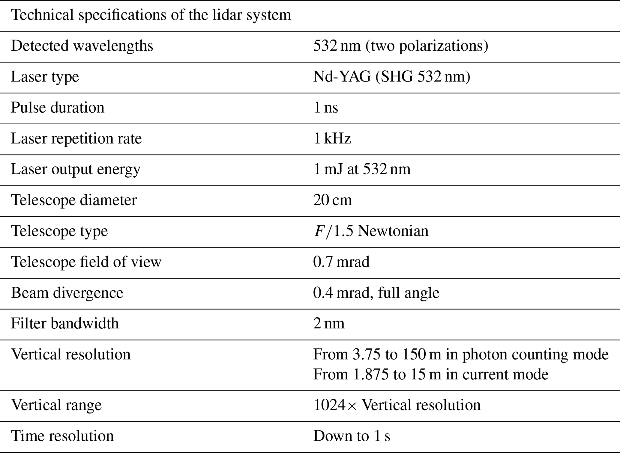
The lidar deployed in Palau is a version of a small, portable, homemade instrument already described in Cairo et al. (2012). Similar systems are designed to work unattended in remote sites and have been used in previous campaigns in Africa (Cavalieri et al., 2010, 2011) and Europe (Di Liberto et al., 2012; Rosati et al., 2016; Bucci et al., 2018). We will briefly describe the setup used in this work. The system is contained in a $\mathrm{30}\times \mathrm{40}\times \mathrm{50}$ cm aluminium box that is electronically shielded and thermally insulated with polyurethane. An inclined quartz window on its top allows the transmission of the laser beam and the collection of the backscattered signal. The temperature in the aluminium box is controlled by four 20 W cooler–heater Peltier cells; an additional 200 W Peltier cell conditioner was added to improve the temperature control in equatorial conditions. The laser source (Bright Solutions, Wedge) is an air cooled, diode-pumped Nd-YAG with second-harmonic generation and active Q switching. The laser pulse duration is 1 ns and the emission is at 532 nm (green) with energies of 1 mJ/pulse. The pulse repetition rate is 1 kHz. The laser beam divergence is reduced to 0.4 mrad by a beam expander and the laser is aligned to the telescope field of view (FOV) by a steerable dielectric mirror placed before the beam expander. The telescope is Newtonian with a diameter of 20 cm, $f/\mathrm{1.5}$ with a FOV of 0.75 mrad. The overlap of the laser beam with the FOV begins at 40 m from the instrument and is completed at 600 m. An overlap correction function O(r) is used to reconstruct the backscatter signal over that region (Biavati et al., 2011). Narrow band interference filters with 5 nm bandwidth, high transmission and negligible temperature dependence select the backscattered light from the sky background. A cube polarizer is used to further divide the radiation at 532 nm in the components parallel and perpendicular to the polarization of the emitted light. Additional polarizers are placed in front of the detectors, which are miniature photomultiplier modules (Hamamatsu 6780-20) with low thermal noise (less than 10 counts/s at 25 ^∘C). A characterization of crosstalk between the channels was performed following the method outlined in Snels et al. (2009) and found to be negligible. The photomultiplier signals are amplified with a bandwidth of 250 MHz, then recorded both in current and in photocounting mode by an acquisition card (Embedded Devices, APC-80250DSP). The two records can be merged during data processing. In current mode, the photomultiplier signal is filtered through a 15 MHz low pass to avoid aliasing and then digitized into an 8 bits waveform at adjustable sampling rates. The sample duration can be set to 12.5, 25, 50 or 100 ns and the waveform is reconstructed from 1024 samples, providing a spatial resolution from 1.875 to 15 m and a spatial range from 1.875 to 15 km. The system was carefully checked for linearity throughout the measurement dynamical range. An absolute calibration of the channels gain ratio was also performed before the deployment following the procedure outlined in Snels et al. (2009). In photon counting mode, the photoimpulses that are above an adjustable threshold are counted in 1024 consecutive time bins whose length may be set from 25 to 1000 ns in 25 ns increments, providing a spatial resolution from 3.75 to 150 m and a spatial range from 3.75 to 150 km. The dead time estimated from the maximum photon counting rate is 6 ns and its effects are taken into account following Donovan et al. (1993). In both modes, the first 24 bins are collected before the laser shot and used for measuring background light. The acquisition card provides the sum of the signals integrated over a user defined time interval that can range from 1 s to possibly several tens of hours. Data are stored in the memory board of the system. An external computer is used to access the system via a USB or TCP/IP connection. A visualization of the measurements in real time is possible for system checking or for alignment. A synopsis of the system specifications is reported in Table 1. In the Palau campaign configuration, the system was set pointing up vertically to operate every night for 10 h, providing 5 min averaged vertical profiles of atmospheric elastic backscattering with a vertical resolution of 30 m, extending from the ground up to 30 km.

Table 1 Lidar specifications

2.2 Data processing

In elastic lidars, the two physical quantities of interest, the particle backscattering β_a(r) and extinction α_a(r) coefficients, must be determined from the elastic backscatter equation:

$$\begin{array}{}\text{(1)}& \begin{array}{rl}& P\left(r\right)={\displaystyle \frac{\text{EC}}{r^{\mathrm{2}}}}\text{O}\left(r\right)\left[{\mathit{\beta }}_{\text{a}}\left(r\right)+{\mathit{\beta }}_{\text{m}}\left(r\right)\right]\exp \\ & \left(-\mathrm{2}\underset{\mathrm{0}}{\overset{r}{\int }}\left[{\mathit{\alpha }}_{\text{a}}\left(s\right)+{\mathit{\alpha }}_{\text{m}}\left(s\right)\right]\mathrm{d}s\right),\end{array}\end{array}$$

where P(r) is the power of the backscattered radiation received by the lidar telescope from range r, E is the transmitted laser-pulse energy, C is the lidar constant including its optical and detection characteristics, O(r) is the overlap function and β_m(r) and α_m(r) are the molecular backscatter and extinction coefficient respectively that can be derived by meteorological data of air density and molecular scattering theory. To determine the two unknowns, the particle backscattering β_a(r) and extinction α_a(r), a relationship must be assumed between them, often in the form of a constant extinction-to-backscatter ratio, the so-called lidar ratio (LR). This parameter is an intensive aerosol property, strongly depending on its size, shape and composition.

The backscatter ratio (BR), defined from the particle (a) and molecular (m) backscattering coefficients as

$$\begin{array}{}\text{(2)}& \text{BR}={\displaystyle \frac{{\mathit{\beta }}_{\text{a}}+{\mathit{\beta }}_{\text{m}}}{{\mathit{\beta }}_{\text{m}}}}\end{array}$$

is then derived with the Klett inversion method (Klett, 1985) with LR assuming piecewise constant values in regions where clouds or different typologies of aerosols were present. To identify such regions, the values of BR, altitude and volume depolarization ratio δ are iteratively inspected during processing. The volume depolarization ratio δ is defined as

$$\begin{array}{}\text{(3)}& \mathit{\delta }={\displaystyle \frac{{\mathit{\beta }}_{\text{a}}^{\text{cross}}+{\mathit{\beta }}_{\text{m}}^{\text{cross}}}{{\mathit{\beta }}_{\text{a}}^{\text{par}}+{\mathit{\beta }}_{\text{m}}^{\text{par}}}},\end{array}$$

where par and cross refer to the backscattered light with polarization respectively parallel and orthogonal to that of the laser. These values are iteratively inspected during the data processing to recursively adjust the LR accordingly. For instance, when thin liquid or ice clouds are identified, LR is set to values known from the literature to respectively 19 sr (Chen et al., 2002) and 29 sr (O'Connor et al., 2004). The LR for aerosols may easily range from 20 sr in the case of marine aerosol (Papagiannopoulos et al., 2016) to 80 sr for biomass burning aerosol (Weinzierl et al., 2011). We used a constant aerosol lidar ratio set to 26 sr where no clouds were present (Dawson et al., 2015). The values of β_m were retrieved from temperature and pressure profiles (Collis and Russell, 1976) by co-located radiosoundings, which were launched twice a day by the Weather Service Office of Palau and accessible through http://weather.uwyo.edu/upperair/sounding.html (last access: 1 March 2018).

The calibration altitude for BR was chosen typically between 8 and 12 km when free of aerosol and clouds. We set the calibration value of BR to 1.02, as suggested in Kar et al. (2018). The uncertainty associated with the data from the lidar used in this study is extensively discussed in Cairo et al. (2012) and Rosati et al. (2016). At a given altitude, it depends on the attenuation of the signal from the ground, which is affected by low-level clouds and aerosol. For the present purposes, a typical upper limit to the absolute random errors on BR and δ in the tropospheric range may be quantified to be 0.1 and 5 % respectively.

An independent evaluation of the cirrus extinction, and hence of the cirrus LR, was implemented following the approach of Young (1995), obtaining the value of the cloud transmittance determined from the elastically scattered lidar signals from clear regions below and above the cloud. When this approach does not produce results, due to the optical thickness being too small or the noise of the profile being below and/or above the cloud, a fixed value of LR = 29 sr was assumed (Chen et al., 2002). The choice of LR has an effect on backscattering and extinction retrievals. The distribution of our retrieved LR is almost evenly dispersed around the fixed value LR = 29, ranging from 20 to 40 sr. If we take such variability as an estimation of the LR uncertainty the retrieval of the backscatter coefficient may be considered sufficiently accurate, also looking at the fact that the optical thickness involved is often low. Similar considerations apply to the particle depolarization. On the contrary, the extinction retrieval and thus the optical depths are more affected by LR as their relationship with LR is linear. So both extinction and optical depths can be inaccurate up to a factor of 2.

Multiple scattering should be considered when cirrus clouds are analysed. The effect depends on the lidar FOV and on the optical thickness of the clouds, which increase when the two get larger and become nonnegligible when τ approaches unity. It tends to produce observed extinctions and depolarization respectively smaller and greater than the real (effective) ones; the effect on the backscattering coefficient tends to be less important (Bissonnette, 2005). Different correction algorithms have been proposed (see for instance (Eloranta, 1998; Hogan, 2006)), although corrections or adaptations of single scattering retrieval algorithms to take into account multiple scattering effects are not straightforward. We have followed the procedure suggested in Chen et al. (2002): multiplying our τ and the retrieved LR by a multiple scattering factor η given by

$$\begin{array}{}\text{(4)}& \mathit{\eta }={\displaystyle \frac{\mathit{\tau }}{e^{\mathit{\tau }}-\mathrm{1}}}.\end{array}$$

In our case, η was calculated iteratively by applying the correction to the observed τ multiple times until the consistency between the real and observed τ and η was achieved. In our analysis, the η correction ranges from close to 1 in very thin clouds to 0.58 for the thickest ones, which are however a small portion of our data. This latter value can be taken as the order of magnitude of the possible bias on the largest optical depths due to multiple scattering effects. No corrections were made to the backscattering and depolarization coefficients. In fact, the effect of multiple scattering in depolarization is to increase the observed depolarization as the penetration of the lidar pulse into the cloud increases. We inspected the cloud depolarization profiles and found no systematic increase with altitude within the cloud. We therefore considered the effect of multiple scattering in our depolarization, and even more so on backscattering, to be negligible.

The inversion of the lidar data delivers profiles of BR and hence of the particle backscatter coefficient β_a and volume depolarization δ. From the latter, a value of the particle depolarization δ_a can be obtained following Cairo et al. (1999). The uncertainty associated with δ_a very much depends on the associated BR and in our data can be as large as 100 % for a single measurement on very thin clouds. However this uncertainty is the result of random errors that do not produce a bias in the mean values of the measurements. The possibility of systematic errors must however be kept in mind, which may be relevant at low values of δ_a and relatively more affected by an inaccurate calibration of BR.

2.3 Data analysis

Threshold values of 1.2 for BR were used to identify the cloud base z_bottom and top z_top as limits for the calculation of the cloud integrated characteristics; clouds were identified as such in an altitude interval in which condition BR > 1.2 was continuously met for at least 150 m. For them, the vertical extension of the cloud Δz and optical thickness τ were computed. The mid-cloud optical altitude z_o, average temperature, average particle depolarization and average potential temperature were computed as weighted averages over the cloud vertical extension, with the weight given by the cloud particle backscatter coefficient β_a. The mid-cloud geometrical altitude z_g is defined as the average of the cloud top and base altitude.

A back-trajectory analysis was conducted to investigate the thermal and convective history of the cloudy air masses. The convective origin of the air masses was analysed making use of the TRACZILLA Lagrangian model (Pisso and Legras, 2008), a variation of FLEXPART (Stohl et al., 2005) that interpolates vertical velocities and heating rate to the position of the parcel from the hybrid grid using log pressure or potential temperature. Each parcel simulation releases a cluster of 1000 back trajectories, representative of a generic aerosol tracer. The release points are computed from the cirrus cloud position from the lidar measurements with a time step of 3 h along the time axis and a vertical sampling of five points equidistant in pressure between the top and the bottom of the cloud. The trajectories are reconstructed back in time for 30 d in a geographical domain covering the whole globe. The meteorological fields at $\mathrm{1}{}^{\circ }\times \mathrm{1}{}^{\circ }$ resolution are taken from the ERA-Interim ECMWF reanalysis at 3 h resolution using diabatic vertical motion. The convective influence is individuated from the 3-hourly brightness temperature (BT) images at 11 µm from the climate quality Gridded Satellite dataset GRIDSAT-B1 (GRIDSAT78 BI) (Knapp et al., 2011). A convective source is therefore individuated when, in a specific geographical bin, a trajectory is travelling below (has a temperature warmer than) a convective cloud top level, selected from the satellite measurement with BT < 230 K, as similarly done in Tzella and Legras (2011) and Tissier and Legras (2016). More details on the trajectory–convective cloud coupling methods can be found in Bucci et al. (2020) and Legras and Bucci (2020). The age of the air masses is computed as the time elapsed between the time of release of the cluster, i.e. at the time of the lidar observation of the air mass, and the convective cloud crossing.

3 Measurements

3.1 Meteorological context

Palau is located on the northwestern edge of the TWP. Its average daily temperature is 28 ^∘C throughout the year with very small changes from season to season. Its weather is influenced by the meandering of the intertropical convergence zone, extending across the Pacific just north of the Equator, and is most intense in the Northern Hemisphere wet season. The main wet season is from May to October, affected by the West Pacific monsoon that brings heavy rainfall, while the driest season is from February to April (Kubota et al., 2005). Winds come from the northeast from December to March, then revert to westerly between May and July, reverting again to northeasterly between September and December.

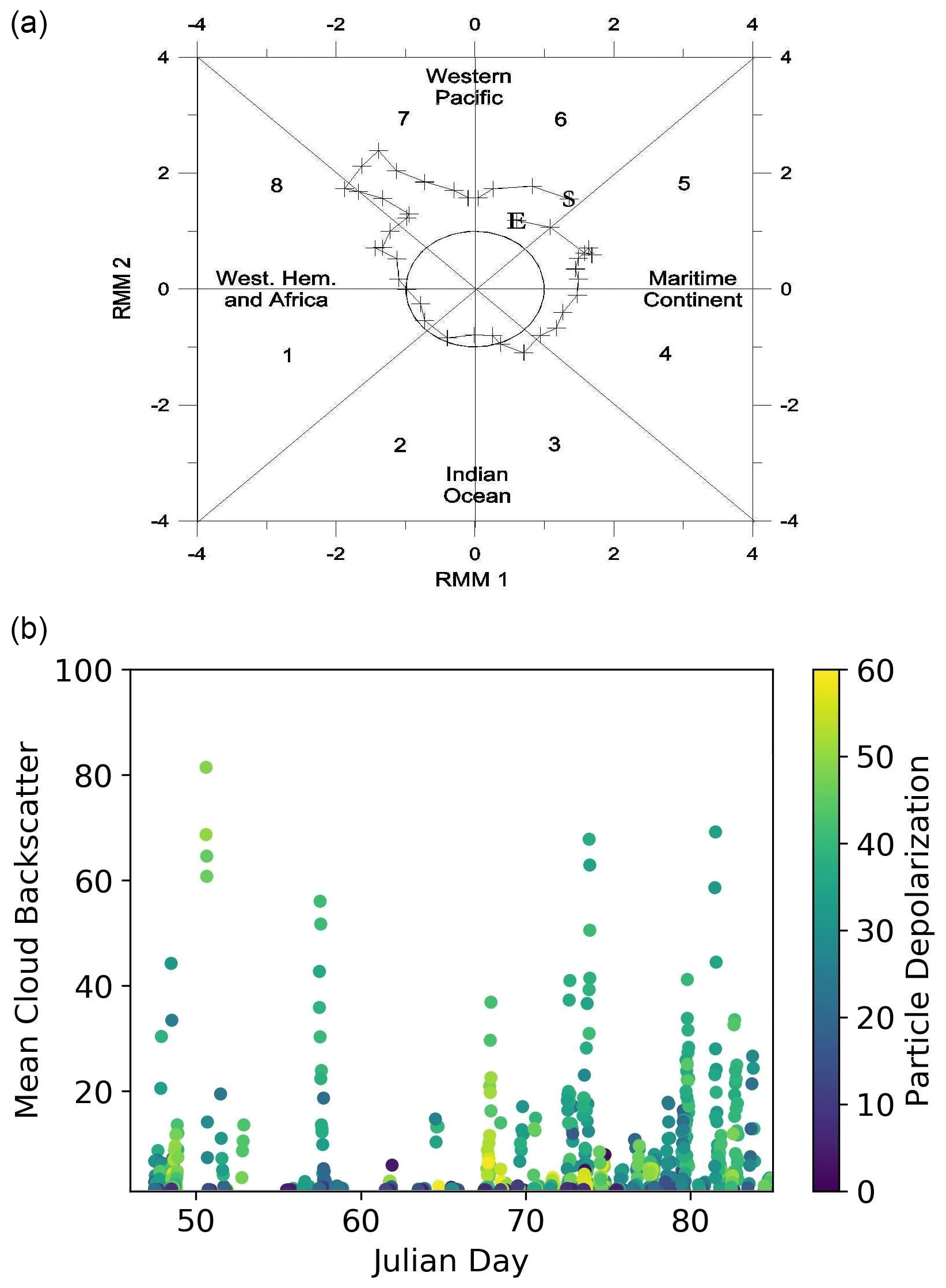
Figure 1 (a) Madden–Julian Oscillation phase diagram for the campaign duration. Start and end days of the campaign are marked respectively with an S and an E. RMM1 and RMM2 data are from the Australian Government Bureau of Meteorology (http://www.bom.gov.au/climate/mjo/, last access: 17 October 2019). (b) Time series of observations of cloud backscatter ratio (BR) during the campaign. The colour codes the particle depolarization. Data points are averages over 300 m of the lidar profile and over 3 h of observations. Observations with BR < 1.2 have not been reported.

The lidar system started operating on 15 February 2016 and stopped on 25 March. That coincided with a whole period of the Madden–Julian Oscillation (MJO), the eastward-moving disturbance of clouds, rainfall, winds and pressure that traverses the tropics in 30 to 60 d on average. The upper panel of Fig. 1 reports the MJO phase diagram during the 50 d of the campaign. Recall that such diagrams represent the magnitude of the first two empirical orthogonal functions RMM1 and RMM2 of the combined fields of near-equatorially averaged 850 hPa zonal wind, 200 hPa zonal wind and satellite-observed outgoing longwave radiation (OLR) data (Wheeler and Hendon, 2004). RMM1 and RMM2 data are from the Australian Bureau of Meteorology website (http://www.bom.gov.au/climate/mjo/, last access: 17 October 2019). Points representing sequential days are joined by a line, and their distance from the origin is related to the strength of MJO cycle. Their position with respect to the eight quadrants into which the diagram is divided indicates the geographical region in which the MJO phase brings an increase in convection. Labels S and E on the diagram marks the beginning and end days of our field campaign. According to that, we should have expected an enhanced convection in the second half of the campaign.

Clouds were observed throughout the campaign, with a prevalence in the second part as depicted in the lower panel of Fig. 2, where a time series of clouds observation is reported; each point represents the average of BR within clouds on a 3 h time window. Colour codes the same average for the particle depolarization.

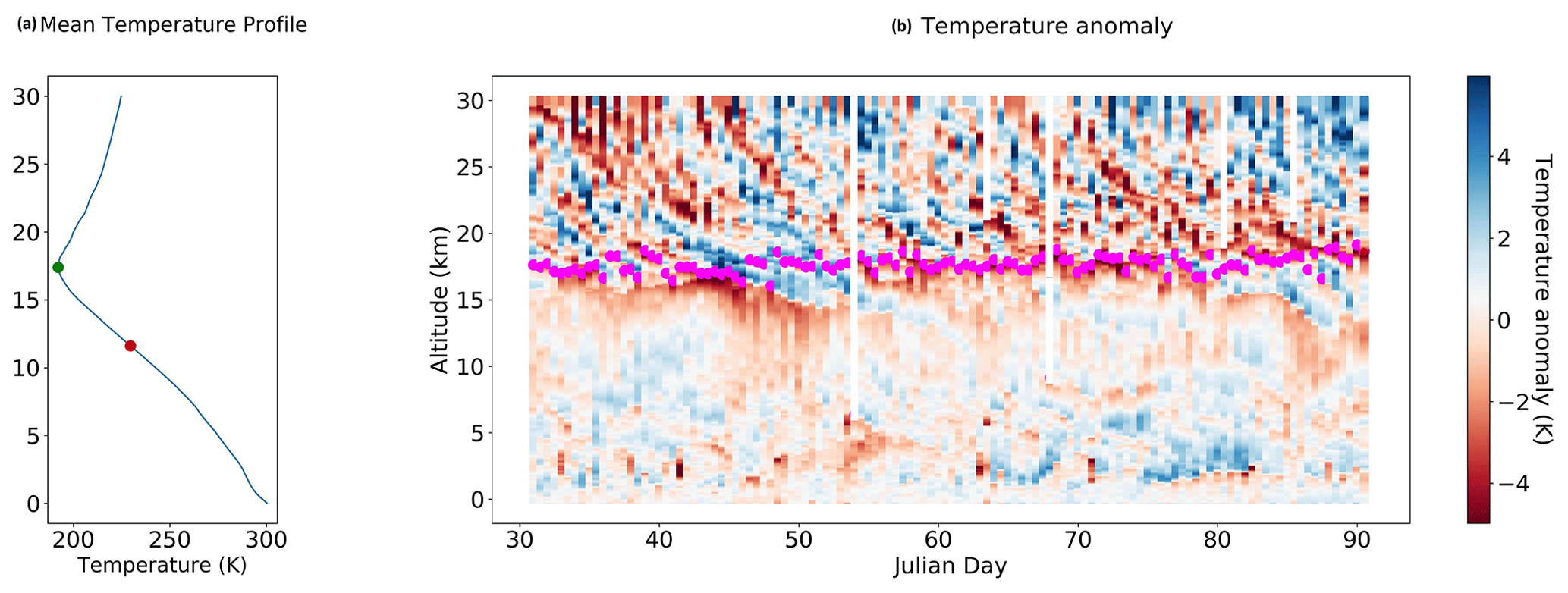
Figure 2 (a) Average temperature profile during the campaign timeframe. The green dot marks the cold-point tropopause (CPT) at 17 400 m and the red dot marks the level of neutral buoyancy at 11 600 m. The tropical tropopause layer (TTL) can be considered to be within these two limits. (b) Temperature anomaly with respect to the average temperature profile on the left. Data are from 12 h radiosoundings routinely launched by the Weather Service Office of Palau from Koror, Palau (station 91408) downloaded from: http://weather.uwyo.edu/upperair/sounding.html (last access: 1 March 2018). Purple dots mark the cold-point tropopause.

Figure 2 reports the average vertical temperature profile (left panel) during the campaign time frame. On average, the cold-point tropopause (CPT) temperature is 192 K at 17 400 m at 382 K potential temperature on average; that altitude is nearly coincident with the lapse-rate tropopause (LRT), defined as the level at which the lapse rate becomes less than 2 K/km and the average lapse rate is less than 2 K/km for 2 km above this level. The level of neutral buoyancy (LNB), which we consider to be the one at which the potential temperature equals the equivalent potential temperature at the ground, is at 11 600 m at 348 K potential temperature on average. In our case it can be shown that this level coincides with the level of minimum stability (LMS), where the vertical gradient of the potential temperature attains a minimum and thus can be taken as the lower boundary of the TTL (Sunilkumar et al., 2017).

On the left panel of the figure the time series of temperature anomaly profiles observed during the campaign are reported. The altitudes of the CPT (purple dots) are also displayed. The pronounced wavefronts in the stratosphere that are seen to descend from the stratosphere and sometimes penetrate below the CPT are the result of large-scale tropical wave activity. We can see here how the structure and variability of the TTL are greatly affected by these fluctuations induced by such gravity waves or Kelvin waves that influence tropopause height, temperature and cloud occurrence (Fueglistaler et al., 2009).

Prevalent winds were from east, veering south with altitude and becoming southerly close to the tropopause.

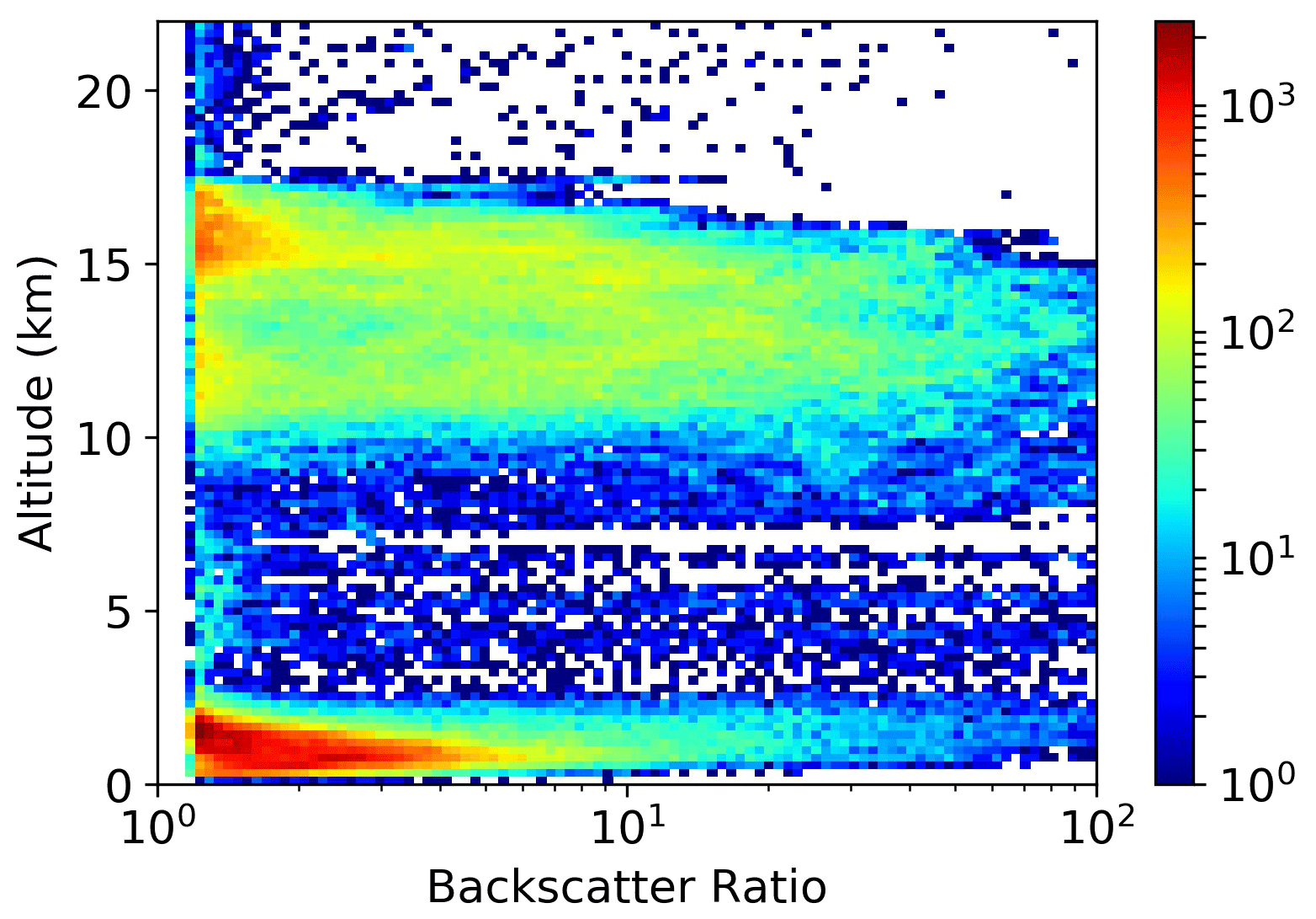
Figure 3 Distribution of backscatter ratio observations vs. altitude. Data are 10 min averages of lidar vertical profiles with 30 m vertical resolution. The colour codes the number of samples in each bin. Only data with BR > 1.2 have been reported.

3.2 Cloud vertical distribution, morphology and optical properties

Figure 3 reports the distribution of BR > 1.2 observations with respect to altitude. Each observation is a 10 min average over an altitude interval of 30 m. Low-level cloud top extends up to 2.5 km, then a relatively clear altitude range is observed. High-altitude clouds, which are the ones we will focus our attention on, appear from 10 km upward, with two peaks of maximum occurrence respectively at 12 km and at 15 km; then, their occurrence tapers off until the tropopause is reached.

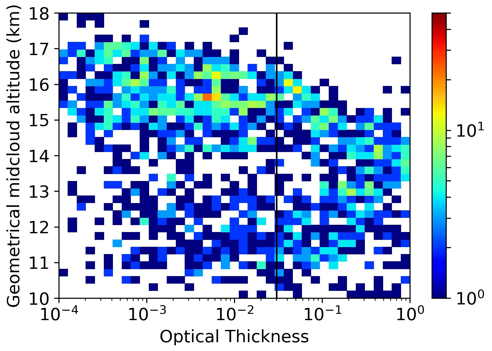
Figure 4 Distribution of cloud optical thickness observations vs. mid-cloud altitude. The colour codes the number of samples in each bin. The thick black line reports the optical thickness threshold value for SVC.

Figure 4 reports the statistics of cloud optical thickness vs. geometrical mid-cloud altitude. Here and in the figures that follow, the reported data are from 10 min averages of lidar vertical profiles with 30 m vertical resolution, and a cloud is defined as an altitude interval not thinner than 150 m where the conditions BR > 1.2 and the signal to noise ratio is lower than 0.5 on the parallel channel are continuously met. The continuous vertical line indicates the τ value that separates altostratus and thin cirrus from subvisible cirrus (τ<0.03). Most of our observations are SVC, mainly collected between 15 km and the tropopause; the distribution of the SVC has a second maximum in the lower part of the TTL, between 11 and 13 km altitude. The thin cirrus clouds are distributed more evenly in altitudes up to 15 km, with a slight tendency to get thicker with increasing altitude; no significantly thick cirrus are present in the tropopause. In Fig. 5 the statistics of τ vs. the geometrical cloud thickness Δz are shown. In spite of the wide spread of the data, an almost linear increase of τ with Δz is apparent, with two different slopes respectively for the SVC and thin cirrus classes. The vertical distribution of backscattering inside the cloud was also investigated (see Fig. S2 in the Supplement for further details). In many cases, the lower and upper parts of the cirrus appear to produce the same scattering effect for small to medium values of τ, indicative of an even distribution of backscatter inside, which we may be taken as a proxy for the distribution of IWC. Conversely, the thickest clouds tend to have lower backscatter in their bottom part with respect to the top part, with a few exceptions for the highest ones; this is arguably due to mass redistribution by sedimentation.

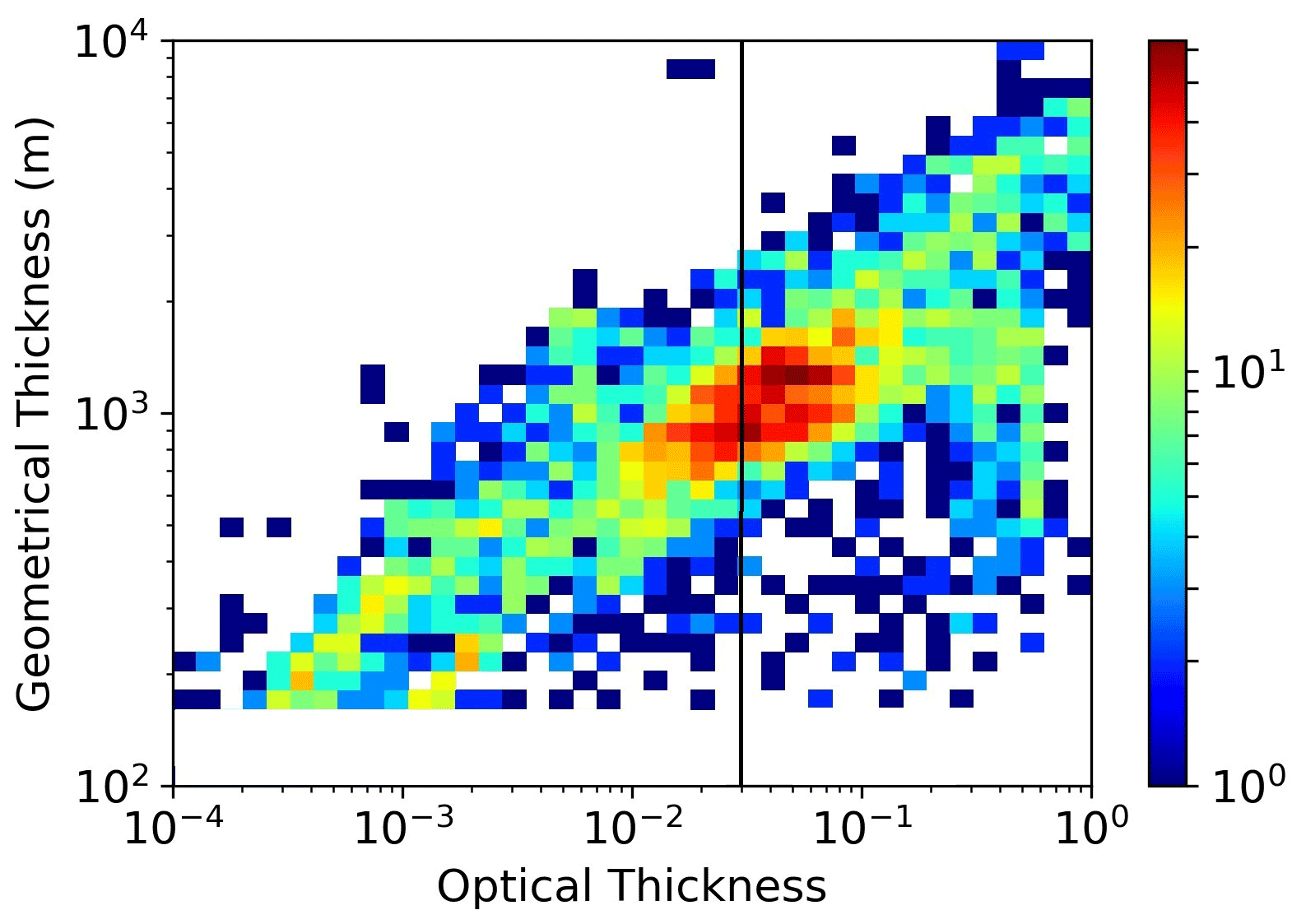
Figure 5 Distribution of cloud optical vs. geometrical thickness. The thick black line reports the optical thickness threshold value for SVC. The colour codes the number of samples in each bin.

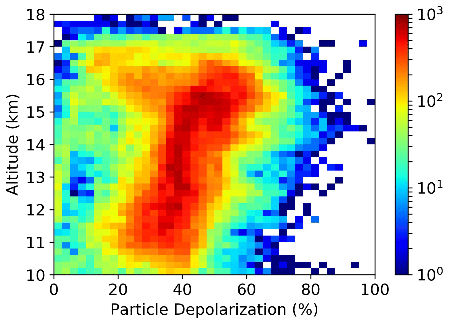
Figure 6 Distribution of particle depolarization vs. altitude. Data are 10 min averages of lidar vertical profiles with 30 m vertical resolution. The colour codes the number of samples in each bin. Only data with BR > 1.2 have been reported.

The trend of particle depolarization with altitude, i.e. with decreasing temperature (see Fig. S1 in the Supplement), shows a compact linear relationship with a progressive increase towards higher altitudes, as shown in Fig. 6. This linearity is apparent from 10 km to slightly below the tropopause. It is interesting to note that when approaching the tropopause, a different behaviour sets in between 15 and 17 km such that an entire range of depolarization values is also observed. It is possible to show that the data associated with the compact linear increase of depolarization toward higher altitude are associated with particle backscatter coefficients β_a covering the entire range of their variability (in our data, between 10⁻⁸ and 10⁻⁴ m⁻¹ sr⁻¹). Conversely, those depolarization data at high altitude, which are almost evenly distributed between 10 % and 60 %, are associated only with medium to low values of β_a. In particular, particle depolarization values below 20 % start to appear when the temperature drops below 200 K, and at temperatures around 190 K they reach values as low as 10 %, which are atypically low for cirrus clouds and have been observed in association with the lowest values of β_a. Very low values of δ_a can be observed in presence of large oriented crystals in clouds, typically planar crystals with their main faces aligned horizontally (Platt et al., 1978; Noel and Sassen, 2005). However, we have to acknowledge the fact that our observed low values can be relatively more affected by an inaccurate signal calibration process that may in turn induce inaccuracies in the determination of particle depolarization. We have estimated that these inaccuracies are no greater than 50 % of the reported value for the aerosol depolarization. This is an upper limit, as the inaccuracy uncertainty greatly reduces when aerosol depolarization values are accompanied by high backscattering.

The fact that different optical typologies of clouds coexist in the upper part of the TTL can also be seen by inspecting the relation between the cloud-averaged values of the particle depolarization δ_a and optical thickness τ, as shown in Fig. 8. There, two branches can be discerned: for medium to high values of τ associated with thin cirrus, those arguably topping at 15 km in Fig. 4, there is a decreasing trend of δ_a vs. τ, while for small to medium values of τ associated with SVC, the particle depolarization is more spread through its variability range. The analysis of the LR obtained with the Young procedure shows that in the majority of cases LR is distributed between 20 and 40 sr with a peak around 30 sr and without showing particular dependencies on the mean depolarization, temperature or optical thickness of the cloud (see Figs. S3, S4 and S5 in the Supplement).

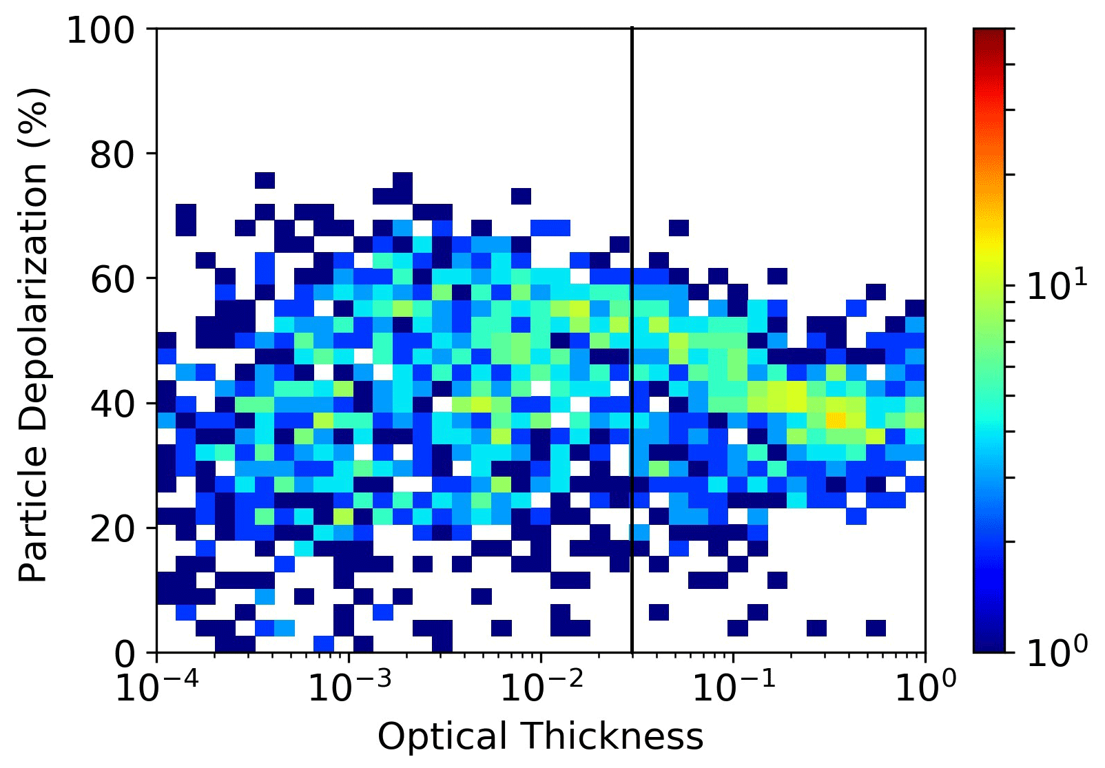
Figure 7 Distribution of cloud-averaged values of particle depolarization vs. optical thickness. The thick black line reports the optical thickness threshold value for SVC. The colours code the number of data points falling inside the bin.

3.3 Clouds close to the tropopause

It is worthwhile zooming in on what happens close to the tropopause; therefore, we move to a reference system centred at the altitude of the CPT, and we replot the statistics of the particle depolarization data with respect to the distance from the CPT in Fig. 8. Again, we are able to see the presence of two modes in the depolarization, which are particularly evident from 2 to 1 km below the tropopause and around the tropopause; one has high values and one has medium to low values of depolarization. It is worth noting that clouds, especially those with medium to low depolarization values, do not extend significantly above the CPT. In Fig. 9, for the same subset of observations depicted in Fig. 8, we report the statistics of the simultaneous occurrence of particle depolarization and local temperature anomalies, the latter calculated as deviations of the temperature profile measured by the concomitant radiosounding with respect to the average temperature profile during the campaign, as reported in the right panel of Fig. 2. It is evident that cloud occurrence is associated with cold-temperature anomalies. It is noteworthy that clouds with high depolarization are present throughout the whole variability range of cold anomalies, while those with medium to low depolarization occur only when the temperature drops 2 to 3 K below the average. It can be shown that such a correlation between cloud occurrence and negative temperature anomaly is not present for clouds at lower levels.

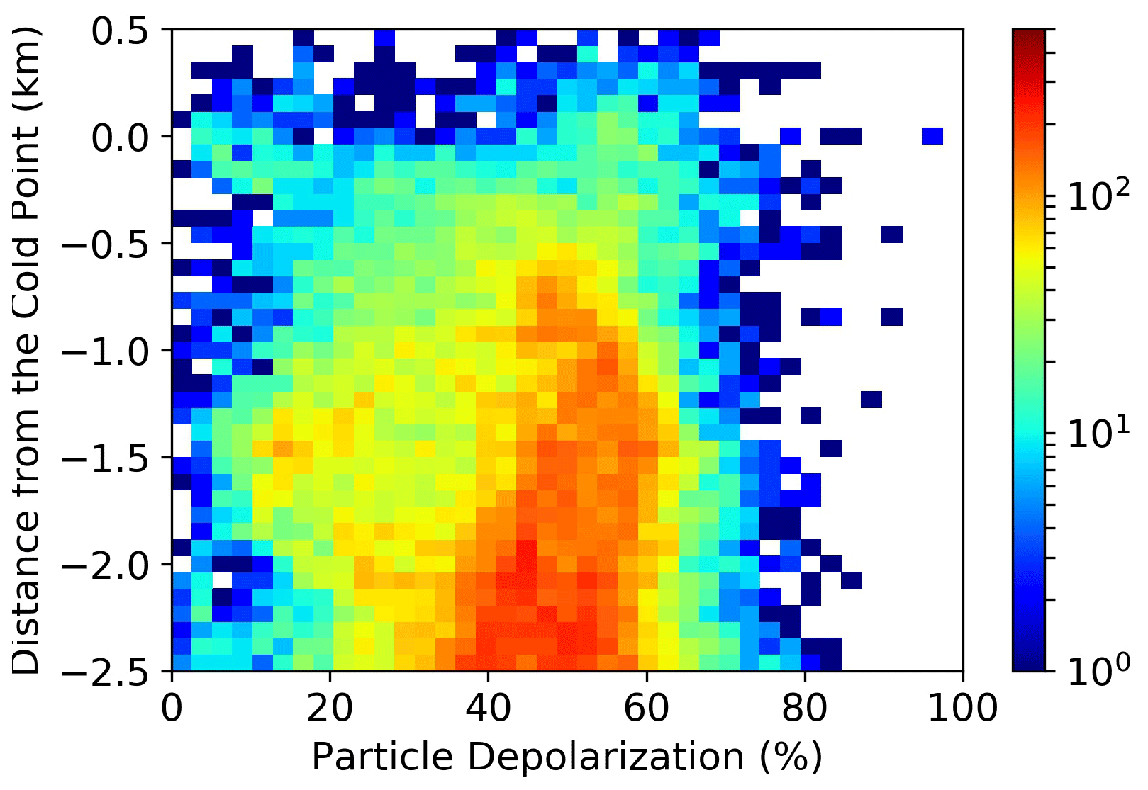
Figure 8 Distribution of particle depolarization observations vs. distance from the cold-point tropopause. Data are 10 min averages of lidar vertical profiles with 30 m vertical resolution. The colour codes the number of samples in each bin. Only data with BR > 1.2 have been reported.

4 Trajectory analysis

The trajectory analysis allows possible linking of the optical characteristics of the clouds with the thermal and convective history of the air mass. Clusters of 1000 trajectories were launched backward from the altitude and time of the cloud observations, and the averaged trajectory over each cluster, together with its dispersion, was used for further analysis. Along each of the averaged back trajectories, the minimum temperature encountered, T_min, and the time elapsed since that, t(T_min), was computed together with the derivatives of temperature $\mathrm{d}T/\mathrm{d}t$, potential temperature $\mathrm{d}\mathit{\theta }/\mathrm{d}t$ and pressure $\mathrm{d}p/\mathrm{d}t$ at the time of lidar measurements, computed as averages over the past 18 h. Moreover, the following quantities were also computed: the time during which the air mass remained below the temperature attained at the lidar observation t(T(t)<T₀), the minimum potential temperature θ_min, the maximum pressure p_max and the relative times elapsed from the lidar observation t(θ_min) and t(p_min).

For each averaged back trajectory, the “convective fraction” – defined as the percentage of the trajectories in the cluster that had met convection – was also computed. The time elapsed since the most probable convection encounter was defined as the time from the maximum increase of the convective fraction in the cluster. In Fig. 10 the points represent the encounters of the retro-trajectories with convective episodes. The colour codes the time elapsed since the convective event; Palau is indicated by a red dot. Recent convection is present south and east of Palau, off the coast and east of Papua New Guinea. Older convective episodes are scattered along the tropical belt, extending into the Indian, Pacific and Atlantic oceans as far as into the Gulf of Guinea. The information obtained from the analysis of the retro-trajectory was connected to the measured optical parameters: depolarization, optical thickness and LR.

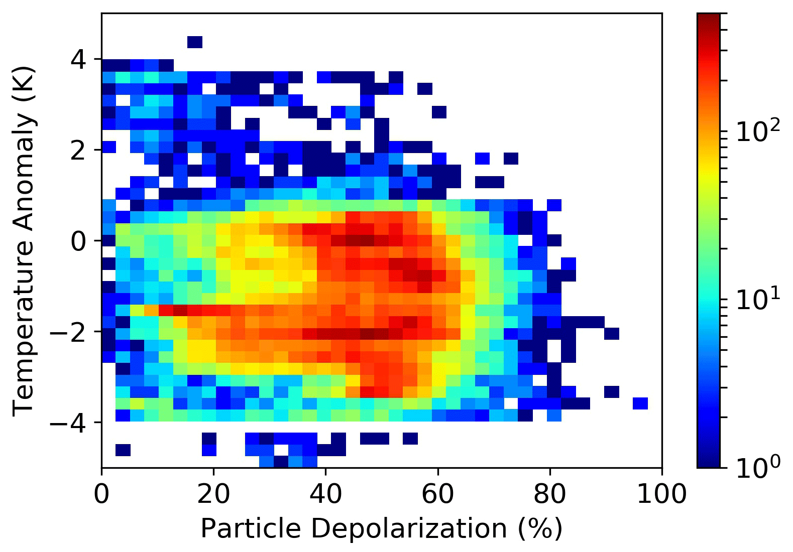
Figure 9 Distribution of particle depolarization observations vs. temperature anomaly with respect to the average temperature profile as reported in the left panel of Fig. 2. Only data of clouds from 2500 m below to 500 m above the CPT are reported. Data are 10 min averages of lidar vertical profiles with 30 m vertical resolution. The colour codes the number of samples in each bin. Only data with BR > 1.2 have been reported.

Most of the clouds in the upper part of the TTL are stationary or experience a slight warming, while some of those in the lower part, especially among the thickest ones, are cooling. The temperature differences along the back trajectories are below 5 K for many of the clouds, with a few exceptions for clouds in the mid-TTL between 12 and 15 km, with medium to high optical thickness and medium to low depolarization, which experienced temperature differences as large as a few tens of Kelvin.

The clouds encountered their minimum temperature T_min less than 48 h before observations; therefore, relatively recently with a few exceptions for clouds below 14 km with high optical thickness and medium to low depolarization for which the temporal distance from the minimum of temperature along the back trajectory was as large as 100–200 h. Generally, the clouds spent less than 48 h below the temperature T₀, which is indicative of relatively recent origin, with the exception of some clouds present both in the upper part of the TTL and below 14 km, which spent several days below T₀.

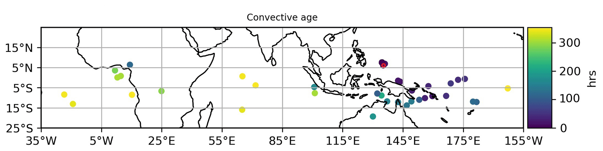
Figure 10 Geographical and temporal distribution of convective influences on observations. The dots indicate the positions in which the retro-trajectory has encountered convection. The colour indicates the time elapsed since that event with respect to the observation in Palau. Palau is indicated with a red dot.

A more interesting picture came from the analysis of the maximum potential temperature difference along the trajectory, indicative of the altitude jump: while for clouds below 16 km this difference is smaller than 10 K, above that level θ_max−θ_min is consistently greater, ranging from 15 to 25 K. In fact, above that altitude the potential temperature gradient begins to assume stratospheric characteristics. Moreover, the clouds in the TTL and particularly in its upper part had met θ_min several days before the observation, while on the contrary, in the back trajectories from clouds at lower levels θ_min was temporally significantly closer to the observations, going back to some hours up to 1 or 2 d before.

The convective influence on the cloud air mass spans between 20 % and 60 %, evenly spread across altitude, somewhat larger for the highest and optically thinnest clouds. The time elapsed from the most likely convective encounter is below 2 d, except for very few cases, scattered throughout the altitude range, when it is greater.

It is worthwhile noting that the high-level SVC with low optical thickness and depolarization have the highest potential temperature difference along the back trajectory and the longest time interval from θ_min and below T₀, possibly suggesting an origin other than the recent convection one.

5 Discussion

Previous studies (Massie et al., 2010; Sassen et al., 2008, 2009; Nazaryan et al., 2008) based on satellite data have shown that cirrus cloud frequency over the tropics, and over the TWP in particular, is higher during the northern winter. Furthermore, cirrus clouds in the upper troposphere tend to be more frequent at night, especially on land, despite the fact that no clear diurnal pattern in deep convective activity is seen. A similar diurnal cycle is not observed for SVCs present near the CPT. Virts and Wallace (2010) have studied the annual, interannual and intraseasonal variability of TTL, based on 3 years of CALIPSO observations. They found an influence of deep convective clouds, modulated by the seasonally varying Hadley cell and monsoons and the year-round oceanic convergence zones, on cirrus in the 12–15 km layer. Interestingly, they have found that TTL cirrus over the Maritime Continent and western Pacific are significantly correlated with convective activity approximately 30^∘ of longitude to the west, suggesting that convection may also exert an indirect influence on TTL cirrus formation by forcing vertically propagating planetary waves in addition to the direct influence through the spreading of cumulonimbus anvils. The low-level influence tapers off as one ascends through the TTL, where the variability in the TTL cirrus at levels above 15 km begins to reflect the character of the stratospheric circulation with frequency higher throughout the tropics during the boreal winter, modulated by Kelvin-like, and to a lesser extent Rossby-like, planetary wave perturbations. MJO-related deep convection can induce planetary-scale Kelvin and Rossby waves in the stably stratified TTL. Regions of ascent in these waves are associated with enhanced cirrus occurrence, as pointed out by Virts and Wallace (2014), who also observed anomalies in temperature, radiative heating rates, carbon monoxide and ozone, propagating eastward and circumnavigating the tropical belt over a roughly 40 d interval.

Our analysis, based on night observations, shows how cloud occurrence extends throughout the whole TTL with two defined peaks, one at 10–13 km and the other at or slightly below the CPT. Although both the region and the time of year were the most favourable for observing cirrus clouds above the CPT (Zou et al., 2020), in our observations clouds do not extend significantly above that level. It is noteworthy how only the upper TTL clouds are largely affected by local atmospheric temperature anomalies. Our observational period covers a whole MJO cycle, with enhanced convective activity at the beginning and at the end of it. During these periods the clouds observed were thicker and higher. Moreover, they often appeared in more than one layer with the lowest layer between 10–13 km of altitude. Conversely, during the less active period of the MJO, clouds were mostly observed only in the upper part of the TTL. Luo and Rossow (2004), coupling satellite observations with Lagrangian trajectory analysis, showed that the decay of deep convection is immediately followed by the growth of cirrostratus and cirrus, the latter continuously evolving, thinning out and moving to lower levels. They were able to estimate an average lifetime of 1–2 d so that clouds can be advected on scales of several hundreds of kilometres. As their occurrence seems to be in phase with an enhancement of convection due to the MJO phase, it is tempting to attribute our observations of clouds in the lower part of the TTL to convective activity.

In our observations, depolarization increases with height and generally decrease with temperature, as already reported in other observations (Wang et al., 2020; Sunilkumar and Parameswaran, 2005). In the upper part of the TTL, depolarization may vary over a wide range, with some of the highest and thinnest SVC clouds attaining medium to low depolarization. In situ measurements, reviewed in Lawson et al. (2019), have shown that particle shapes in fresh anvil outflows are markedly different from those in in-situ formed cirrus, the latter showing a prevalence of bullet rosettes and polycrystals, virtually absent in the convective cirrus dominated by single crystals and aggregates of crystals: plates, double plates, columns and irregulars with some needles, stellars and dendrites. This difference reflects different formation mechanisms, as ice may form in convective updraughts prior to reaching the homogeneous freezing level (−38 ^∘C). Cirrus from aged outflows have intermediate characteristics. Moreover, in the upper part of the TTL where in situ formation is likely predominant, measurements in SVC show the prevalence of small quasi-spheroids and plates, in concentrations of 1–10 cm⁻³, while in the lower part of TTL where cirrus can more likely be generated by convection, particles are bigger and attain lower concentrations.

Some of the observed SVC may have had rather long lifetimes and are associated with negligible lifting in the hours preceding the observation. The study of the convective influence is not conclusive, so we may speculate that this class of SVC may have originated by in situ formation with nucleation processes that induce morphologies, sizes and concentrations of ice crystals that differ from those that we can observe at lower altitudes (11–13 km) where the depolarization and the optical thickness is higher. Such in situ formation may be triggered by the activity of tropical waves that may induce temperature anomalies as large as 2–3 K close to the CPT, while the clouds in the lower part of the TTL, which more likely originated by convective events, are dependent on local temperature conditions only for their subsistence and not for their formation. The analysis shows how cloud occurrence extends throughout the whole TTL with two peaks, one at 10–13 km and the other at or slightly below the CPT; clouds do not extend significantly above it. It is noteworthy that only those upper TTL clouds are largely affected by local atmospheric temperature anomalies.

6 Conclusions

Five weeks of night lidar observations of equatorial cirrus clouds were presented and their morphology and optical and geometrical characteristics were discussed, also in the light of a trajectory analysis aimed at connecting their properties with the thermal and convective history. The lidar-derived depolarization shows a linear increase with altitude up to the top of the troposphere, where a full range of depolarization values is present. For a subset of these high-altitude clouds with low depolarization and optical thickness values, the absence of recent significative uplifting in the histories of those air masses suggests a mechanism of formation by in situ condensation, triggered by temperature fluctuation. Conversely, the majority of cirrus in the TTL have thermal and convective histories compatible with formation from convective outflows, bringing up moisture and ice. In the thickest of them, the negative difference between the optical and geometrical mid-cloud altitude gives a hint that larger ice crystals are being removed from the TTL by sedimentation, leaving smaller particles on optically thinner cirrus that can survive for several hours. The fact that the presence of small particles in cirrus particle size distributions increases in percentage with decreasing temperature, i.e increasing altitude, and with increasing time since convective influence has been reported by Woods et al. (2018). Compared to observations in other climatically important regions, observations of equatorial cirrus in the TWP are scarce, so this work, albeit limited to lidar observations during a relatively short time frame, contributes to enriching the observations. The work would have benefitted from the simultaneous use of balloon hygrometers to better explore the effect of cirrus clouds on the distribution of water vapour in the TTL. An observational campaign with balloon hygrometers and the deployment of the more performing lidar COMCAL by the Alfred Wegener Institute will help to better define the morphology and microphysical processes in the TTL in this region.