The impact of volcanic eruptions of different magnitude on stratospheric water vapor in the tropics

Increasing the temperature of the tropical cold-point region through heating by volcanic aerosols results in increases in the entry value of stratospheric water vapor (SWV) and subsequent changes in the atmospheric energy budget. We analyze tropical volcanic eruptions of different strengths with sulfur (S) injections ranging from 2.5 Tg S up to 40 Tg S using EVAens, the 100-member ensemble of the Max Planck Institute – Earth System Model in its low-resolution configuration (MPI-ESM-LR) with artificial volcanic forcing generated by the Easy Volcanic Aerosol (EVA) tool. Significant increases in SWV are found for the mean over all ensemble members from 2.5 Tg S onward ranging between [5, 160] %. However, for single ensemble members, the standard deviation between the control run members (0 Tg S) is larger than SWV increase of single ensemble members for eruption strengths up to 20 Tg S. A historical simulation using observation-based forcing files of the Mt. Pinatubo eruption, which was estimated to have emitted (7.5±2.5) Tg S, returns SWV increases slightly higher than the 10 Tg S EVAens simulations due to differences in the aerosol profile shape. An additional amplification of the tape recorder signal is also apparent, which is not present in the 10 Tg S run. These differences underline that it is not only the eruption volume but also the aerosol layer shape and location with respect to the cold point that have to be considered for post-eruption SWV increases. The additional tropical clear-sky SWV forcing for the different eruption strengths amounts to [0.02, 0.65] W m⁻², ranging between [2.5, 4] % of the aerosol radiative forcing in the 10 Tg S scenario. The monthly cold-point temperature increases leading to the SWV increase are not linear with respect to aerosol optical depth (AOD) nor is the corresponding SWV forcing, among others, due to hysteresis effects, seasonal dependencies, aerosol profile heights and feedbacks. However, knowledge of the cold-point temperature increase allows for an estimation of SWV increases of 12 % per Kelvin increase in mean cold-point temperature. For yearly averages, power functions are fitted to the cold-point warming and SWV forcing with increasing AOD.

1 Introduction

It has been established that the entry of water vapor into the stratosphere is largely controlled by the temperature of the tropical tropopause (e.g., Brewer, 1949; Mote et al., 1996; Fueglistaler et al., 2009; Dessler et al., 2014). Following up on the discussion of the long-term increasing trend in stratospheric water vapor (SWV) observed during the 1980s and 1990s, it was proposed that volcanic eruptions could be influencing the SWV budget (e.g., Rosenlof et al., 2001; Joshi and Shine, 2003). Mainly, two processes are considered: the direct volcanic injection from the volcanic plume and an indirect volcanic mechanism due to an increase of the tropopause temperature, referred to hereafter as the indirect volcanic pathway. The increased SWV levels may remain in the stratosphere for more than 5 years (Hall and Waugh, 1997), even though the volcanic aerosols sediment out of the stratosphere within 1–3 years (Robock, 2000). However, the magnitude of the SWV increase and the contribution from the different entry mechanisms are still unclear.

In total, 80 % of the eruption material is water vapor (Coffey, 1996), which could be directly injected into the stratosphere during an eruption event. But although the SWV originating form the direct injection can be detected shortly after the eruption event, it is a singular event. The corresponding elevated SWV levels are spread in the stratosphere and are not distinguishable from the background SWV anymore. Satellite evidence for the direct injection events exist. It is discussed briefly by Schwartz et al. (2013) and in depth by Sioris et al. (2016a, b). Based on a model study, Joshi and Jones (2009) hypothesized that the environment surrounding the plume can also have a significant impact on the amount of SWV injected directly.

This study will focus on the indirect volcanic entry mechanism. In contrast to the direct entry, it can act for months or even years after volcanic eruptions since it depends on the heating caused by the aerosol layer in the stratosphere and not on the eruption event itself. This indirect volcanic entry is caused by the terrestrial longwave and near-IR solar heating by the volcanic aerosol layer which leads to increased cold-point temperatures. Consequently, the saturation water vapor pressure at the cold point is increased, thereby reducing the loss of WV due to ice formation and fallout. This mechanism enhances the entry of WV into the stratosphere. In an early idealized study, Joshi and Shine (2003) underlined the importance of the aerosol profile and corresponding heating in the tropopause region. Despite the mechanisms being known, its analysis is still complicated, as internal variability and scarcity of observations have made it difficult to observe it in practice. Additionally, even if SWV increases are recorded, the data usage might be discouraged, as was the case for Mt. Pinatubo by the Stratospheric Aerosol and Gas Experiment II (SAGE II) because discrepancies between different satellites could not be satisfactorily explained (Fueglistaler et al., 2013). The scarcity of observational data is also reflected in the quality of the available reanalysis products for SWV, the usage of which in general is discouraged in some papers (e.g., Davis et al., 2017) and which sometimes do not implicitly account for the volcanic forcing at all (Diallo et al., 2017; Tao et al., 2019). The latter problem was also indicated by Löffler et al. (2016) when discussing SWV increases simulated for the eruption of Mt. Pinatubo. Nevertheless, by performing a regression analysis using a trajectory model fed by reanalysis data, Dessler et al. (2014) identified a SWV peak partially overlapping with the aerosol optical depth (AOD) signal of Mt. Pinatubo. As the SWV increase occurred before the eruption and AOD increase, the question remained if the peak in the residual might instead be caused by another source of variability. Another possible issue in their analysis is that some of the effects modeled by the regressors are themselves influenced by volcanic eruptions, which may lead to the volcanic signal being attributed to a different source. An example are the increases of the Brewer–Dobson circulation (BDC), which, in the case of a volcanic eruption, can be partially caused by the heating due to the aerosol layer. Tao et al. (2019) also undertook an indirect quantification of the SWV increase after volcanic eruptions via another regression analysis, explicitly accounting for volcanic source terms. They found a clear volcanic signal in the expected time frame, but the magnitude of the SWV increase differed strongly between the individual reanalysis data sources.

After entering the stratosphere, the additional SWV affects both stratospheric chemistry with respect to ozone loss (Robrecht et al., 2019; Rosenlof, 2018; Tian et al., 2009) and SO₂ oxidation (Bekki, 1995; LeGrande et al., 2016), as well as the radiative budget of the entire atmosphere (Solomon et al., 2010). Despite the forcing originating from the additional SWV often being mentioned as a motivation for studies, few studies exist on the forcing effect of the SWV increase after volcanic eruptions. Independent of volcanic eruptions, Forster and Shine (2002) analyzed the forcing impact of SWV changes in an artificial SWV profile. In a study focusing on the Mt. Pinatubo eruption, Joshi and Shine (2003) calculated the additional global forcing originating from the post-eruption SWV increase. As this was a side study of their paper, they did not investigate the temporal evolution nor the impact of different eruption strengths. In a study on the direct injection, Joshi and Jones (2009) quantified the longwave component of the SWV forcing indirectly, but their setup did not allow for a quantification of the additional contribution of the indirect volcanic pathway. Most recently, Krishnamohan et al. (2019) attributed changes in their top-of-atmosphere (TOA) imbalances for different geoengineering scenarios to a large influence of SWV. However, they did not separate the contributions of aerosol forcing and SWV.

So far, the questions remain open as to what the critical magnitude is for an eruption to have a significant impact on SWV content, what the radiative consequences of the SWV increase are, and if these effects can be predicted based on eruption magnitude or AOD. In this study, we therefore investigate the changes in stratospheric water vapor originating from the indirect volcanic pathway using a large ensemble of coupled climate model simulations with 100 ensemble members each for five eruption strengths described by changing amount of stratospheric sulfur and a control run, called EVAens (Azoulay et al., 2021). The idealized setup using forcing files generated with the Easy Volcanic Aerosol tool (EVA) offers the unique opportunity of a direct comparison between the different eruption strengths, since the date and location of the eruptions are identical and all ensembles have the same set of starting conditions. By comparison with the control run, a direct quantification of the SWV increase is possible. The large ensemble size allows us to perform an analysis of the sensitivity of the increase in stratospheric water vapor to the eruption strength along with its statistical significance. The critical eruption strengths that cause stratospheric water vapor perturbations beyond the internal variability of the model are identified when analyzing the individual ensemble members.

2 Methods

2.1 The EVAens ensemble and the GE historical simulations

This study is based on large ensemble simulations covering the time frame of January 1991 to December 1993 using two different volcanic forcing data sets: EVAens (Azoulay et al., 2021) and a subset of the Max Planck Institute Grand Ensemble (MPI-GE) historical simulations (Maher et al., 2019). Both ensemble simulations are performed with the Max Planck Institute – Earth System Model in its low-resolution configuration (MPI-ESM-LR) (version MPI-ESM 1.1.00p2). We apply an intermediate model version between the Coupled Model Intercomparison Project phase 5 (CMIP5) version (Giorgetta et al., 2013) and the CMIP6 version (Mauritsen et al., 2019) of MPI-ESM, with a behavior closer to the CMIP6 version. MPI-ESM itself is a coupled model including the atmosphere component – ECHAM (version echam-6.3.01p3; Stevens and Bony, 2013), the land component – the Jena Scheme for Biosphere Atmosphere Coupling in Hamburg (JSBACH; version jsbach-3.00; Reick et al., 2013; Schneck et al., 2013), the ocean component – the MPI Ocean Model (MPIOM; version mpiom-1.6.1p1; Marsland et al., 2003; Jungclaus et al., 2013) and the biogeochemistry component – the Hamburg ocean carbon cycle model (HAMOCC version 5.2; Ilyina et al., 2013). In the model setup, the atmosphere is run in a T63L47 configuration corresponding to a horizontal resolution of about 1.9^∘ with 47 pressure levels up to 0.01 hPa. The influence of the sponge layer in the uppermost model layer reaches down to a height of 65 km with continuously decreasing impact. As MPI-ESM-LR does not include interactive atmospheric chemistry or aerosols, the volcanic aerosols are prescribed by the monthly zonal mean values of their optical properties – the extinction, single scattering albedo and asymmetry factor – in 16 longwave and 14 shortwave bands. During the simulation, these monthly aerosol properties are interpolated linearly in time. In the MPI-GE historical simulations, the optical properties of the volcanic aerosols are prescribed with an updated version of the Pinatubo aerosol data set (PADS) (Stenchikov et al., 1998; Driscoll et al., 2012; Schmidt et al., 2013). The Mt. Pinatubo eruption in June 1991 lies in the investigated time frame.

In EVAens, the setup of the MPI-GE historical simulations was kept, changing only the stratospheric aerosols' representation. The respective forcing files were generated using the Easy Volcanic Aerosol (EVA) forcing generator (Toohey et al., 2016). Six 100-member ensembles were created: a control run with zero sulfur emission only using the EVA background aerosol and five volcanic eruption runs (2.5, 5, 10, 20, 40 Tg S) with both the EVA background aerosol and a volcanic eruptions occurring in June 1991 at the Equator, each with 100 ensemble members. Every ensemble member was started from one of the different and independent runs of the MPI-GE historical simulations in 1991 (Maher et al., 2019). Besides the volcanic aerosols, the forcing files include an aerosol background for the industrialized period supplied by EVA.

The AODs for the five different eruption strengths of the EVA forcing along with the PADS Mt. Pinatubo forcing are shown in Fig. 1 for the 550 nm waveband. All EVA aerosol distributions have very similar patterns but differ in magnitude and duration of elevated AOD levels. Whereas the 2.5 Tg S run returns close to background conditions within 3.5 years after the eruption, the 40 Tg S run only declines to the peak values of the 2.5 Tg S run within this time. The PADS data set has a higher background AOD level than the EVA data sets in the months before the eruption. With a sulfur amount of (7.5 ± 2.5) Tg S (Timmreck et al., 2018), the Mt. Pinatubo AOD should be comparable to the 5 and 10 Tg S EVA data set (compare Table 1). Generally, the AOD in the PADS data set does not spread as fast to higher latitudes after the eruption. Additionally, the AOD values tend to be slightly higher than the values for the 10 Tg S EVA data set and persist longer at elevated levels.

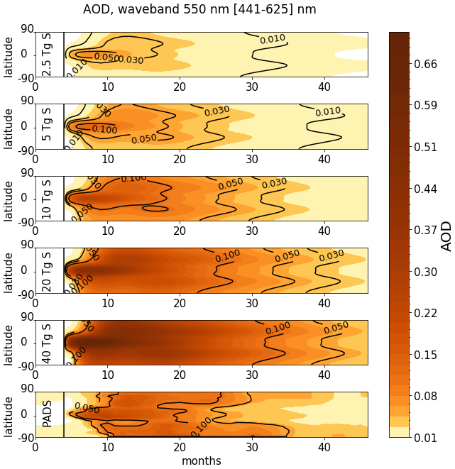
Figure 1 Time evolution of the aerosol optical depth (AOD) for the five volcanically perturbed EVAens runs (2.5, 5, 10, 20 and 40 Tg S) and the PADS Mt. Pinatubo compilation. The zonal average AOD is shown for all latitudes considering the 550 nm waveband (441–625 nm).

Timmreck et al. (2018)Timmreck et al. (2018)Timmreck et al. (2018)Marshall et al. (2018)

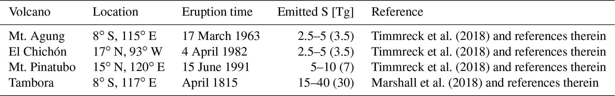
Table 1 List of tropical volcanic eruptions with location, eruption date and estimated amount of emitted sulfur. The sulfur amounts in parentheses represent the best estimates.

As we merely prescribe the aerosols, only the indirect volcanic pathway, which includes cold-point warming and overshooting convection, and not the direct injection or aerosol chemistry is simulated in EVAens. In the following work, all anomalies will be defined as the value difference between the volcanically perturbed (P) and unperturbed 0 Tg S (U) ensemble means (P−U).

2.2 Stratospherically adjusted clear-sky forcing calculations

The stratospherically adjusted clear-sky radiative forcing, as defined by Hansen et al. (2005), originating from the increase of stratospheric water vapor due to the indirect volcanic pathway (i.e., via tropopause warming by the aerosol layer), is calculated using the 1-D radiative convective equilibrium (RCE) model, konrad (Kluft et al., 2019; Dacie et al., 2019). Konrad is designed to represent the tropical atmosphere. It uses the Rapid Radiative Transfer Model for GCMs (RRTMG) and a simple convective adjustment that fixes tropospheric temperatures up to the convective top according to a moist adiabat, whereas the temperatures in the higher atmospheric levels are determined by radiative–dynamical equilibrium. Being a 1-D model, konrad employs a highly parameterized “circulation”, i.e., an upwelling term constant in time which only causes adiabatic cooling. As the temperature above the convective top can adjust, this does not mean that the dynamical heating is fixed (compare Fels et al., 1980).

In order to calculate the stratospherically adjusted SWV forcing, the following procedure is employed: for each eruption strength, including the 0 Tg S eruption, the ensemble mean of the clear-sky humidity profile in the tropical region [$-\mathrm{5},\mathrm{5}$]^∘ latitude is determined from the EVAens output. In order to compute the adjusted radiative forcing due to the increased SWV, the difference between the fluxes in an equilibrated atmosphere with and without the additional SWV must be calculated. To determine the equilibrated reference without additional SWV, konrad is run to equilibrium with the humidity profile and chemical composition of the atmosphere fixed to the values from the 0 Tg S runs. The final surface temperature lies between 298–301 K. Starting from this equilibrium state, only the SWV profile is replaced by the volcanically perturbed EVAens humidity profile and a new equilibrium is calculated while keeping the surface temperature fixed but allowing for the temperature above the convective top to adjust. Using both equilibrium states, the adjusted SWV forcing is determined from the flux differences at the top of the atmosphere. The corresponding instantaneous forcing as defined by Hansen et al. (2005) is calculated as the difference of tropopause fluxes obtained without running the perturbed atmosphere into equilibrium. For the all-sky case, the contribution of clouds is investigated by additionally taking a 20 % fraction of high-level clouds between 200 and 300 hPa into consideration, while low-level clouds are considered in the albedo settings.

In order to relate the SWV forcing to the aerosol forcing, the instantaneous aerosol forcing is calculated using a double radiation call in MPI-ESM. For the double radiation call, fluxes are calculated for each time step once using the atmospheric conditions with and without aerosol. The stratospheric background aerosol is corrected for by additionally calculating the forcing for the corresponding 0 Tg S run and subtracting it.

3 Results

3.1 Effects on the time evolution of TOA radiative imbalance and surface temperature

In order to relate the amount of emitted sulfur to its impact on the energy budget of the system, we analyze the TOA radiative imbalance after the volcanic eruptions as well as changes in surface temperature. The time span of negative global radiative TOA imbalance after the volcanic eruptions, during which more energy leaves the Earth–atmosphere system than is taken up, lasts between 17 and 28 months (Fig. 2). For the lower emissions (2.5–5 Tg S), the standard error of the negative TOA imbalance permanently overlaps with zero imbalance. Consequently, single ensemble members of the 0 Tg S can produce similar signals to these lower emission runs due to internal variability. Overall, the TOA imbalance exhibits a roughly linear relationship with respect to the emitted sulfur mass (see Fig. A1). As a consequence of the negative TOA imbalance, the surface temperatures in the volcanically perturbed runs decrease. The range of ensemble mean maximum global temperature decrease for EVAens is −0.09–1.30 K (Fig. 2). As the surface temperature follows the TOA imbalance, the change in surface temperature is also roughly linear with respect to the emitted S mass (Fig. A2).

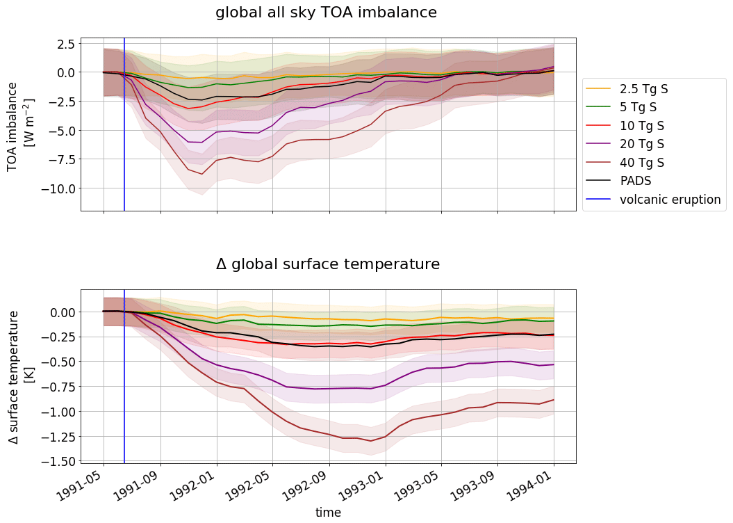
Figure 2 Global top-of-atmosphere (TOA) radiative imbalance and anomaly of surface temperature in the five volcanically perturbed EVAens runs (2.5, 5, 10, 20 and 40 Tg S). For each run, the standard errors of the mean are denoted by shading. The vertical blue line marks the eruption time. The plots also show the values for the MPI-GE historical simulations (PADS).

In addition to the EVAens results, the TOA imbalance and global surface temperature changes for the historical Mt. Pinatubo eruption are shown in black in Fig. 2. The global TOA imbalance, peaking at −2.4 W m⁻², compares favorably with the approximately −3 W m⁻² from Earth Radiation Budget Satellite observations (Soden et al., 2002) when considering the standard deviations of our ensemble. The average surface cooling between June 1991 and December 1993 is −0.26 K, with a maximum cooling of −0.36 K in our simulations, whereas the cooling documented by satellite measurements from the microwave sounding unit (MSU) was −0.3 K between June 1991 and December 1995 after El Niño–Southern Oscillation (ENSO) removal and reached a peak cooling of −0.5 K (Soden et al., 2002).

3.2 Effects on the cold-point temperature

In the following analysis, the cold point is estimated as the lowest temperature in the tropical tropopause layer (TTL) region lying on full pressure levels of model output remapped to a vertical spacing of 10 hPa in the tropical tropopause region. The associated errors in average cold-point temperature lie below ±1.1 K. The effect of the volcanic forcing on the inner tropical temperature profile is visualized in Fig. 3 showing the EVAens ensemble mean of the temperature profiles 3 months after the eruption. The month of September was chosen as an example since it lies in the season of relatively large water vapor entry into the stratosphere due to a maximum cold-point temperature in boreal autumn and winter. Due to the location of the aerosol peak above the cold point, the largest temperature changes occur in the lower stratosphere, with increases up to 24 K in the 40 Tg S ensemble. The cold-point warming reaches maximum values of 8 K in the case of the 40 Tg S run. Also visible in the figure is the downwards shift of the cold point with increasing sulfur burden caused by the stratospheric warming. This effect is amplified by tropospheric cooling (compare surface cooling in Fig. 2) due to the backscattering of solar radiation through the volcanic aerosols.

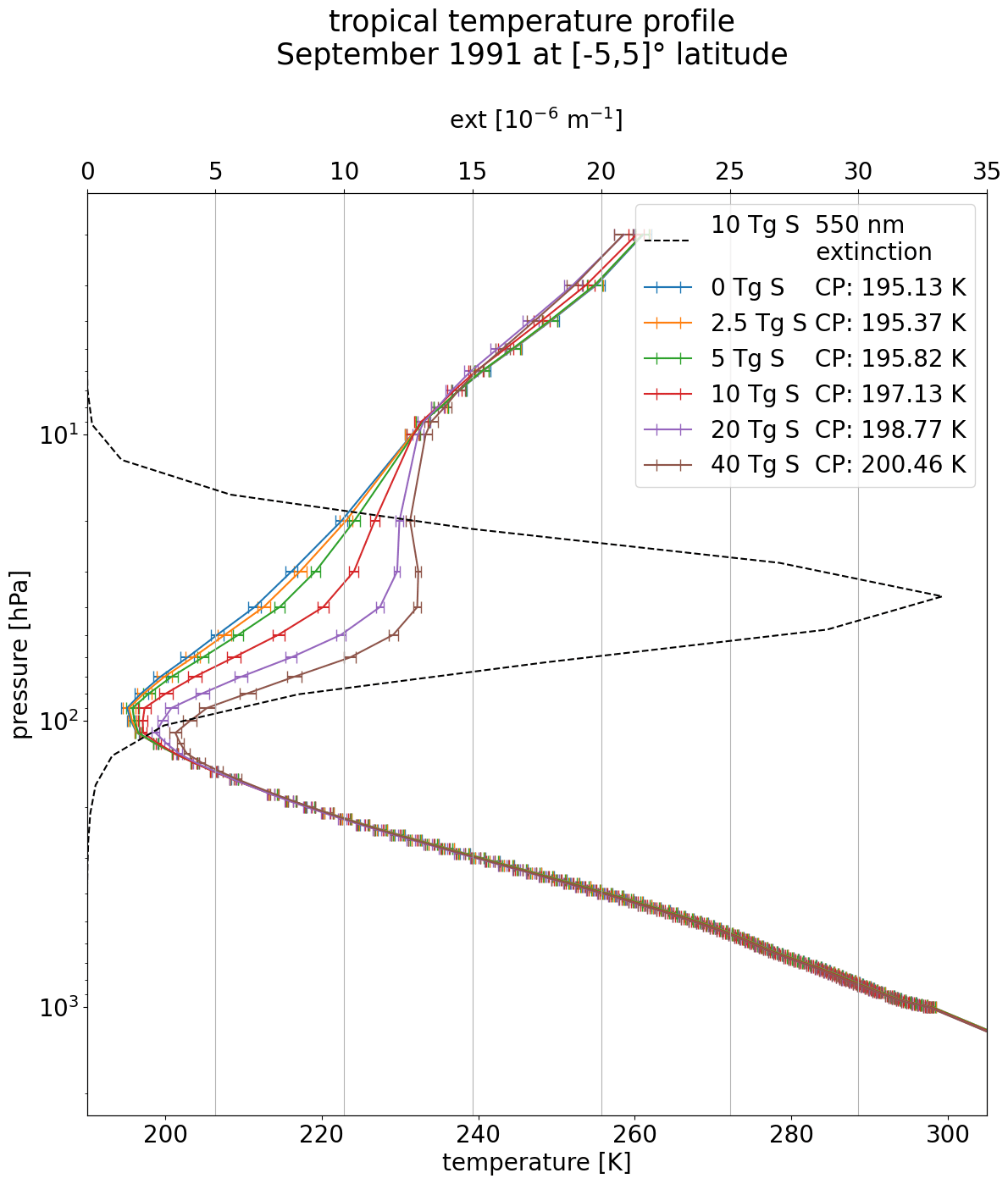
Figure 3 Inner tropical average of the temperature profiles for the five volcanically perturbed EVAens runs (2.5, 5, 10, 20 and 40 Tg S) in September 1991 (3 months after the eruption). The temperature of the respective cold point (CP) is indicated in the legend. The solid line represents the ensemble mean; the error bars symbolize the ensemble standard deviations. The 550 nm extinction values for the 10 Tg S aerosol profile are shown with a dashed black line.

Figure 4 shows the temporal evolution of the surface temperature (a), cold-point temperature (b) and 70 hPa specific humidity (c) as the difference to the zero emission run in the inner tropics. Whereas the surface temperature decreases due to the scattering of incoming shortwave radiation by the volcanic aerosols, the cold-point temperature increases due to warming of the tropopause layer by absorption of terrestrial longwave and solar near-IR radiation by the aerosol layer.

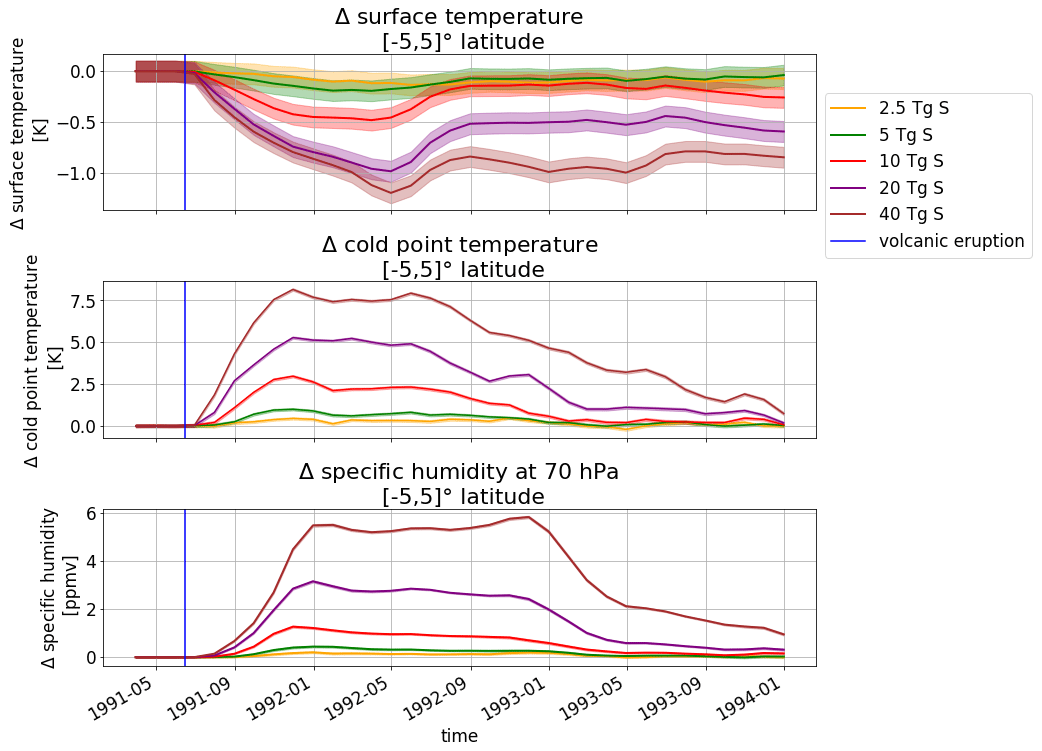
Figure 4 Temporal evolution of the inner tropical mean anomaly in surface temperature, cold-point temperature and stratospheric water vapor between volcanically perturbed and unperturbed ensemble runs. The ensemble means are shown with their standard errors. The time of the volcanic eruption is indicated by a vertical blue line.

When considering the ensemble mean and its standard error, even the temperature changes of the low emission runs (2.5 and 5 Tg S) are significantly different from the control run for short periods of time. With a maximum value of 0.99 K, the ensemble mean for the cold-point temperature of the 5 Tg S is the lowest sulfur emission to reach a mean warming above the control run standard deviations, which are 10 times larger than the standard error for our 100-member ensemble and reach maximum values of 0.73 K. Cold-point values below the standard deviation range could be found for single-control-run ensemble members due to internal variability. The higher emission scenarios (20 and 40 Tg S) have longer periods with cold-point temperature changes above the normally observed internal variability. In addition, the 40 Tg S emission group shows a second amplification peak of the yearly cycle of the cold-point temperatures between May and September 1992.

The monthly changes in cold-point temperature are not linear, neither with respect to emitted sulfur mass nor to AOD in the prominent IR waveband (compare Figs. A3, A4). Additionally, the transient behavior of the volcanic forcing – the buildup phase in 1991, the approximately constant forcing in 1992 and the declining phase in 1993, which also differ between the individual eruption sizes – leads to a hysteretic behavior. Nevertheless, when partitioning the cold-point warmings into these individual phases, the dependence of the cold-point warming on IR AOD can be described with a power function of form aAOD^b+c for the years 1991, 1992 and 1993 (Fig. 5).

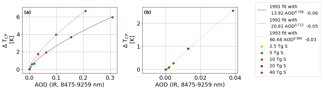
Figure 5 Yearly averages of adjusted tropical cold-point temperature increases as a function of tropical AOD (IR, 8475–9259 nm) for the 3 examined years (1991–1993). A power function fit of form aAOD^b+c for each year with a corresponding equation is shown.

The found cold-point temperature increases are accompanied by an increase in the saturation water vapor pressure, reducing the “freeze trap” drying in the cold-point region. The increased saturation water vapor pressure enables more water vapor to enter the lower stratosphere as shown in Fig. 4c. Consequently, the evolution of the additional stratospheric water vapor closely follows the evolution of the cold-point temperature changes.

3.3 Effects on the tape recorder signal

The manifestation of the annual cycle of the tropical SWV as seen in the vertical profile is often described as the tape recorder signal (Mote et al., 1996): the variations of the tropical cold-point temperatures controlling the water vapor entry into the stratosphere via the saturation water vapor pressure are imprinted on the stratospheric water vapor as music is imprinted on a tape. This leads to an annual cycle of bands of high and low water vapor content propagating upwards in the stratosphere with the BDC. As the heating by the volcanic aerosols will lead to increased tropical cold-point temperatures, an increase of stratospheric water vapor is expected after volcanic eruptions with stratospheric aerosols. As shown in Sect. 3.2, the specific humidity shows an enhancement which does not stay constant and then declines but has an annual cycle like the tape recorder. In the following section, we will investigate the seasonal cycle more closely. Figures 6 and 7 show absolute SWV and the differences in the SWV content above 140 hPa with respect to the control run for all five eruption strengths. The maximum increases are found in the eruption year itself ranging from 0.1 ppmv for the 2.5 Tg S eruption to more than 5 ppmv for the 40 Tg S eruption. This corresponds to 5 % in the case of the 2.5 Tg S simulation and 160 % in the case of the 40 Tg S simulation (see Fig. B1). The larger the eruption, the earlier the increase becomes visible and is significant. The additional SWV also follows the annual cycle of the tape recorder (Mote et al., 1996), showing maxima in the SWV enhancement around September which then propagate upwards. This seasonal variation is also apparent in the behavior of the tropopause and cold-point heights: for scenarios with at least 10 Tg S onward the tropopause pressures and cold-point pressures are higher in the Northern Hemisphere autumn, whereas in the 20 and 40 Tg S runs the volcanic forcing leads to higher pressure levels of the cold point from September 1991 until the end of 1992 accompanied by a seasonal signal in the SWV anomalies. Allowing for more water vapor to transit to the lower stratosphere. In the 40 Tg S ensemble mean, the second seasonal cycle is associated with an upward propagation of the SWV increases above 4 ppmv to even lower atmospheric pressures than in the preceding year. This behavior can be attributed to the persistence of the high levels of aerosols in combination with the already-enhanced SWV levels due to the presence of the aerosol in the previous year, the additional warming caused by the SWV and the lower-lying cold point. Shortly after the eruption, a decrease in water vapor content above 50 hPa is visible. At these altitudes, SWV increases with height due to its production by methane oxidation, which is parameterized in MPI-ESM (Schmidt et al., 2013). Heating in the aerosol layer below leads to lofting of air parcels, bringing lower humidity air upwards to higher altitudes, where it causes a net reduction in humidity. However, this effect never exceeds 0.8 ppmv and is offset as soon as the lifted air becomes more moist due to enhanced SWV entry through the tropopause region.

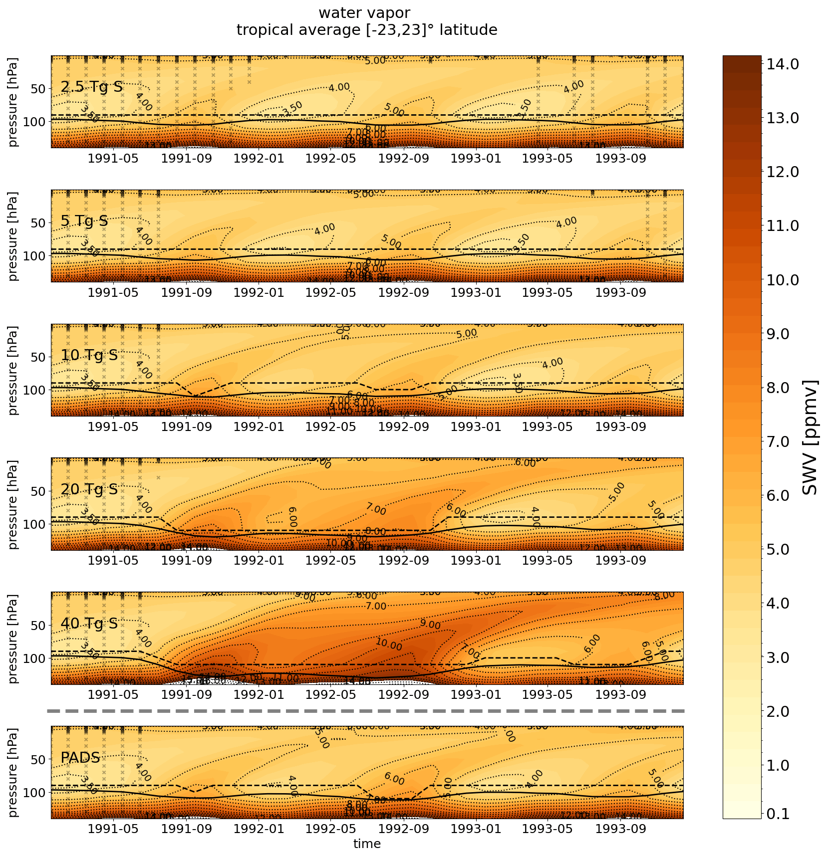
Figure 6 Tropical average in $[-\mathrm{23},\mathrm{23}]$^∘ latitude of WV above 140 hPa for sulfur injections of 2.5, 5, 10, 20 and 40 Tg S as well as the PADS data set. The World Meteorological Organization (WMO)-tropopause pressure is indicated by a black line and the cold-point pressure is denoted by the dashed black line. Absolute values are shown. In regions not covered by black crosses, statistically significant differences between water vapor values of the perturbed and unperturbed runs (t test at p=0.05) were found.

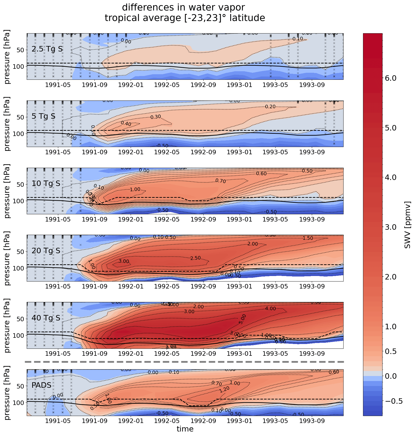
Figure 7 Tropical average in $[-\mathrm{23},\mathrm{23}]$^∘ latitude of WV anomalies above 140 hPa for the sulfur injections of 2.5, 5, 10, 20 and 40 Tg S as well as the PADS data set. The lowermost panel shows the MPI-GE historical simulations for Mt. Pinatubo using the PADS forcing data set discussed in Sect. 3.5. The WMO-tropopause pressure is indicated by a black line and the cold-point pressure is indicated by a dashed black line. Differences with respect to the 0 Tg S control run are shown. In regions not covered by black crosses, statistically significant differences between water vapor values of the perturbed and unperturbed runs (t test at p=0.05) were found.

3.4 Intra-ensemble variability

The investigation of single ensemble members is of interest because – unlike for the ensemble mean – their physical characteristics would actually be “observable”. Figure 8 shows seasonal averages of the specific humidity at the cold point as a function of cold-point temperature for the inner tropical average in 1991 and 1992. The season of September–October–November (SON) was chosen, as it follows the period where the entry value of stratospheric water vapor is highest, leading to the highest SWV in the tropical lower stratosphere. Each point in Fig. 8 symbolizes a single ensemble member. Orange crosses show the theoretically possible maximum specific humidity curve calculated as the saturation humidity for water vapor over ice at the average cold-point temperature, using the corresponding exact solution for the Clausius–Clapeyron equation by Murphy and Koop (2005)¹. An approximation for the Clausius–Clapeyron equation at this temperature range with a 12 % increase of specific humidity per Kelvin is indicated by a dashed gray line. This approximation is based on the assumption that the atmosphere around the cold point is saturated in the 0 Tg S run. The single ensemble members follow the slopes and values of the calculated water vapor amount at saturation in the inner tropics ($[-\mathrm{5},\mathrm{5}]$^∘ latitude). In addition to water vapor, sublimated lofted ice can also contribute to the SWV, leading to higher values than expected based on the saturation water vapor alone. Overshooting events are considered in our convective parameterization (Möbis and Stevens, 2012). However, at the location of the cold point, this lofted ice would still be in the ice state and not accounted for in the specific humidity term. In the inner tropics, the simulated specific humidity values agree nicely with those from the Clausius–Clapeyron equation and its approximated WV dependence on a 12 % increase of SWV per Kelvin. Considering the simplification of taking the average cold-point temperatures between $[-\mathrm{5},\mathrm{5}]$^∘ latitude instead of the minimum cold-point temperatures, this agreement is surprisingly good. Oman et al. (2008), for example, only found good agreement when considering the minimum cold-point temperatures in the tropics. As they were analyzing a band between $[-\mathrm{10},\mathrm{10}]$^∘ latitude, a factor contributing to the difference to our result could be that the main contribution to dehydration of air parcels during their horizontal motion in the vertical ascent takes place in the inner tropics (Schoeberl and Dessler, 2011), the region to which our study is restricted. Consistent with this analysis is the stronger discrepancy of approximately 1.6 ppmv between the SWV values predicted using the Clausius–Clapeyron equation and the SWV output by the model when averaging over the entire tropics (compare Fig. C1).

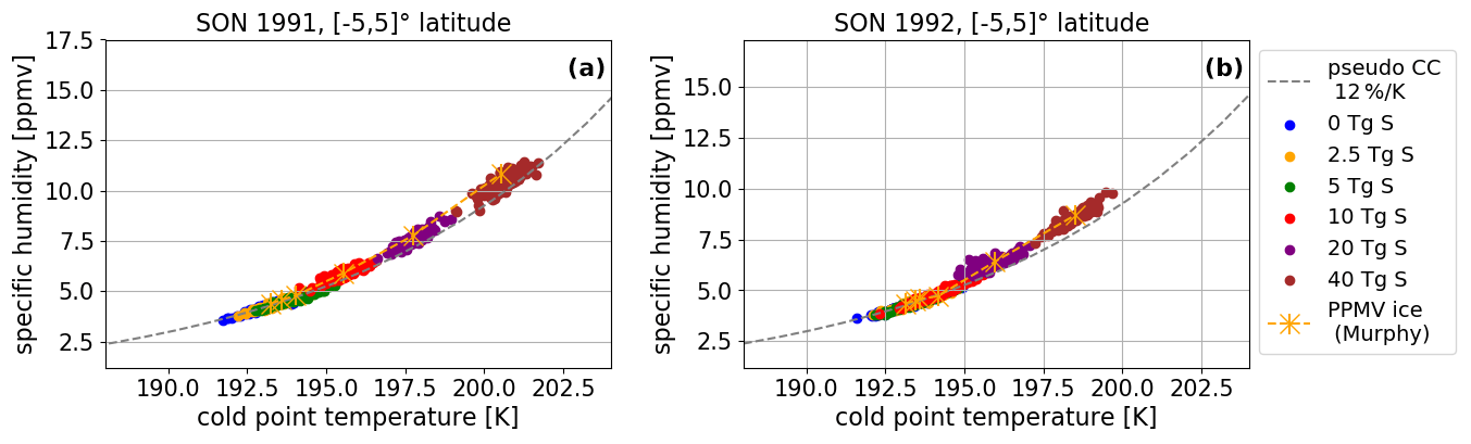
Figure 8 Seasonal averages of specific humidity at the cold point as a function of cold-point temperature for SON 1991 (a) and 1992 (b). Values for each individual ensemble member are shown as dots for the inner tropics. An approximation (see text) for the Clausius–Clapeyron equation at this temperature range with an 12 % increase of specific humidity per Kelvin is indicated by a dashed gray line. The exact solution for the Clausius–Clapeyron equation over ice by Murphy and Koop (2005) is calculated for the average ensemble cold-point temperatures and pressure and shown in orange.

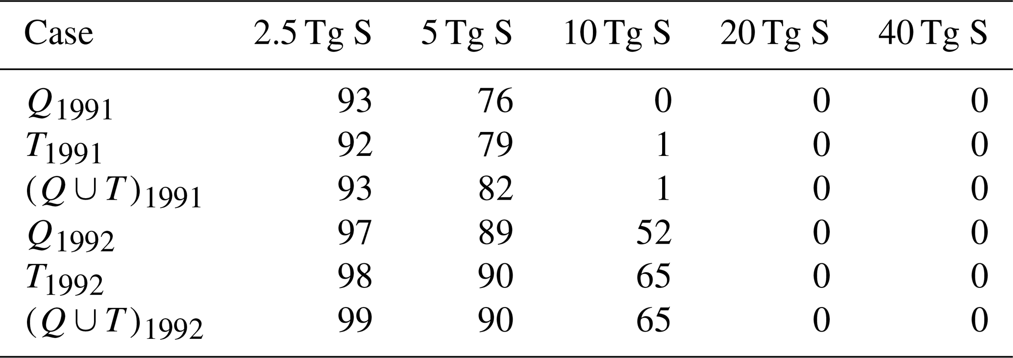
In the first SON after the eruption in 1991, the SWV values and cold-point temperatures are larger than those in 1992. Additionally, the separation by sulfur content is more pronounced in 1991. Table 2 lists the number of individual ensemble members lying within 2 standard deviations of the temperature or humidity value spread of the control run. In 1991, several individual group members up to the 5 Tg S run overlap with the control run spread as far as changes in cold-point temperature and humidity values are concerned. The 10 Tg S run marks the emission strength at which single ensemble members start to be significantly different from the control run as only one ensemble member cannot be distinguished from the control run using only the temperature values. The 20 Tg S run is the first emission strength with no control run overlap and for which all individual ensemble members show a significant increase of SWV content and cold-point temperatures in 1991 and even in 1992 where the lower emission runs start to show an increasing number of ensemble members overlapping with the control run values again. This analysis shows the difficulty to register the SWV increases in observational data which collect data for a single realizations of a volcanic eruption. Although signals similar to those of individual eruptions can be produced by internal variability of an unperturbed scenario, our larger ensemble size allows us to extract a robust signal which may be obscured in a single observational record.

Table 2 Number of ensemble members lying within the 2 standard deviations of the corresponding control run values with respect to temperature (T) or specific humidity (Q) or their union (Q∪T) in 1991 and 1992.

3.5 Comparison to the MPI-GE historical simulations (Mt. Pinatubo)

The importance of the aerosol profile shape and particularly the extinction at the cold point for the SWV entry becomes apparent when comparing the results of the EVAens members to the Mt. Pinatubo period in the MPI-GE historical simulations. In terms of the amount of emitted sulfur, the EVAens simulations for 5 and 10 Tg S can be seen as bounds of recent estimates of the sulfur emission of the Mt. Pinatubo eruption of (7.5±2.5) Tg S (Timmreck et al., 2018). As the PADS data set describing the Mt. Pinatubo eruption is based on observational evidence rather than simulation results, as is the case for the EVA data sets, only a range and not a set amount of emitted sulfur is given. In Fig. 2, which shows the global mean TOA radiative imbalance for the MPI-GE historical simulations along with the EVAens simulations, the values for the Mt. Pinatubo eruption in the MPI-GE historical simulations lie between the 5 and the 10 Tg S imbalances in 1991. In 1992, the mean MPI-GE TOA imbalance is slightly more negative than the ensemble mean of the 10 Tg S run, but overall the deviations between the 10 Tg S run and Mt. Pinatubo run in the MPI-GE historical simulations are small compared to the standard error of the ensemble means.

However, the tropical 1992 SWV anomalies in the historical simulations show a stronger increase than in the 10 Tg S EVAens simulations (absolute values are shown in Fig. 7; for percental changes, see Fig. B1). In particular, the SWV increases show a seasonality enhancing the tape recorder amplitude in the historical simulations which is not present to that extent in the EVAens simulations. Notable is also a stronger SWV increase of 1.2 ppmv in the Mt. Pinatubo simulations of 1992 exceeding the 1.0 ppmv of 1991. The heights the corresponding SWV increases reach also differ: the 0.7 ppmv signal propagates upwards to 20 hPa in the historical run, whereas in the 10 Tg S run the 0.7 ppmv signal only reaches pressure levels of up to 50 hPa.

The higher SWV values are caused by a stronger heating of the atmospheric region around the cold point, controlling the indirect volcanic SWV entry. Figure 9 shows cold-point temperatures for the example of SON 1992. Mt. Pinatubo in the MPI-GE historical simulations reaches values lying between those of the 10 and 20 Tg S run. This can be understood when comparing the aerosol extinction profiles of EVA and PADS as a proxy for the heating generated by the aerosol layer (Fig. 10).

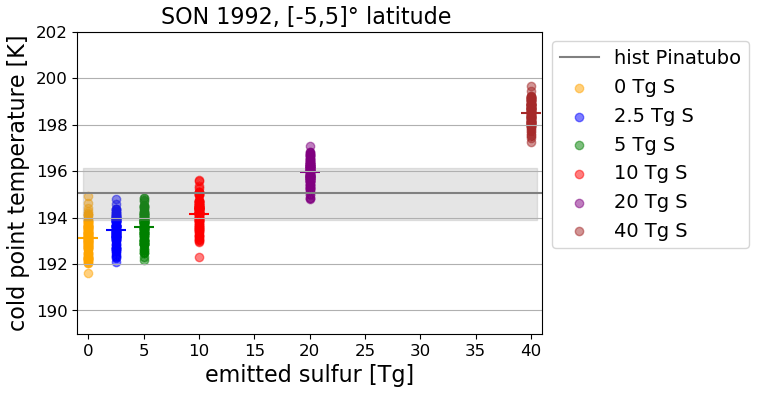
Figure 9 Average cold-point temperature in the inner tropical region $[-\mathrm{5},\mathrm{5}]$^∘ latitude as a function of emitted sulfur for all EVAens members in SON 1992. Each point symbolizes one ensemble member; the horizontal lines denote the ensemble mean. The average cold-point temperature range for the historical Mt. Pinatubo eruptions (PADS) is shown as a gray line; the shaded region shows the extent between corresponding maximum and minimum cold-point temperature.

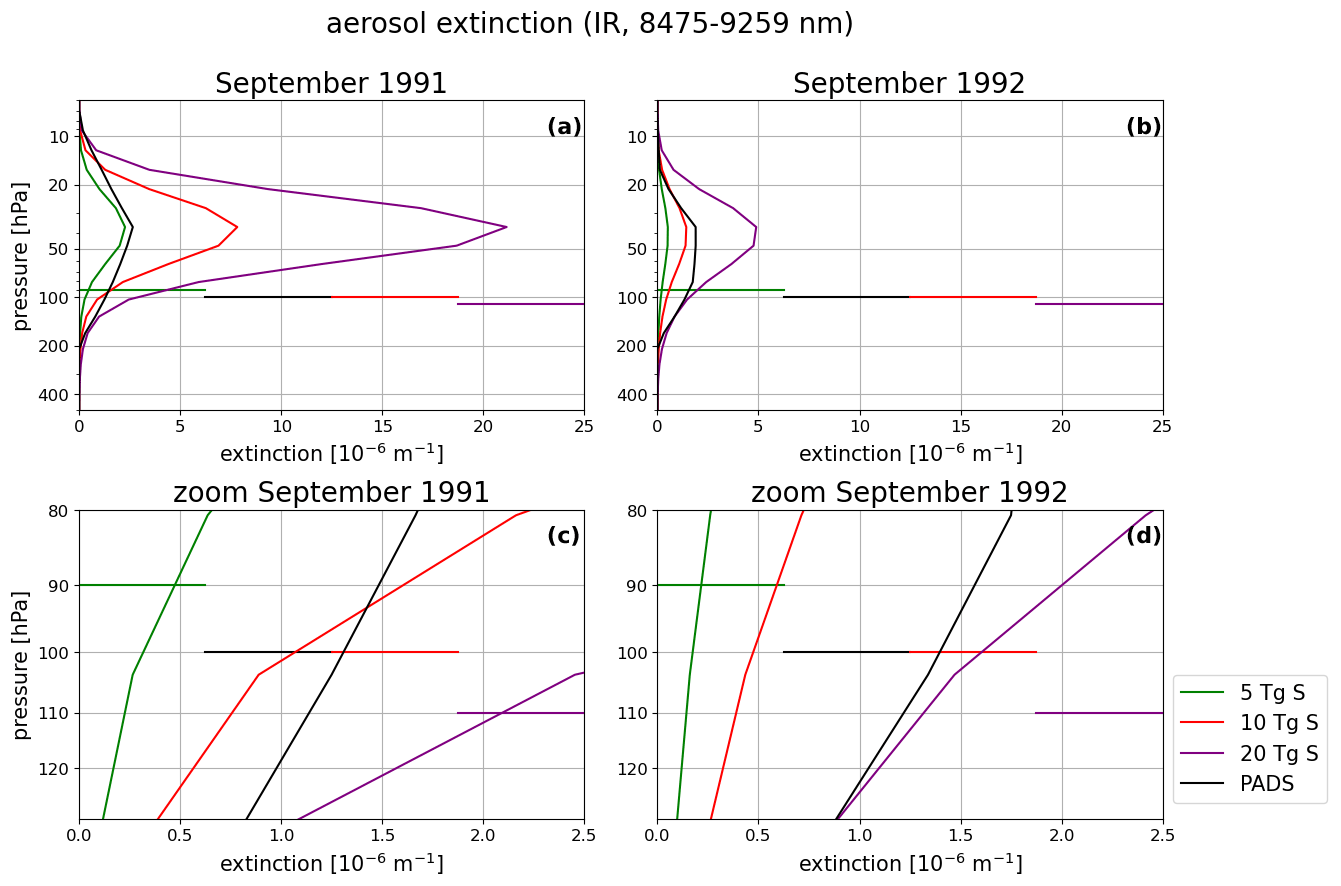
Figure 10 Average tropical aerosol extinction in the 8475–9259 nm infrared waveband from EVA for 5, 10 and 20 Tg S emissions as well as from PADS in September 1991 and 1992. The horizontal lines indicate the pressure levels of the cold point in the region between $[-\mathrm{5},\mathrm{5}]$^∘ latitude for each eruption strength. Panels (a) and (b) show the entire profile. Panels (c) and (d) are zooms of the cold-point region.

Although the PADS data set Mt. Pinatubo forcing has a peak value lying between the 5 and 10 Tg S EVA extinctions, the extinction at the tropopause and cold-point pressure is slightly higher than the 10 Tg S extinction in September 1991 (Fig. 10a and c). In September 1992, the PADS data set reaches values of the 20 Tg S EVA in the cold-point region and a peak extinction comparable to the 10 Tg S profile (Fig. 10b and d). A similar behavior is apparent in the solar extinction bands (see Appendix Fig. D1). As the warming of the cold point determines the SWV entry anomaly, the extinction values at this point will have a significant impact. In 1991, the 10 Tg S EVA extinction values at the cold point are only slightly weaker than the extinction values of the PADS forcing set. The SWV values in the MPI-GE historical simulations are closer, but not equal, to those in the 10 Tg S as the peak extinction values in the 10 Tg S are more than 2 times larger than the PADS extinction values and partially compensate the lower values at the cold point. In 1992, the situation changes, and MPI-GE shows higher SWV values than the 10 Tg S ensemble. The amplification of the SWV entry in the second SON season after the eruption can be attributed to three phenomena. First, the heating was only building up in the Northern Hemisphere summer of 1991 and had not yet reached its maximum value, as can be seen in the plot for the cold-point temperatures (Fig. 4). Second, the peak extinction values of the PADS data set start to exceed the 10 Tg S values in 1992, which may lead to higher SWV entry values (Fig. 11a). Third, the LW extinction at the cold point reaches a second, larger maximum around the northern summer of 1992 with values comparable to 20 Tg S. This second maximum is not represented in the EVA forcing (Fig. 11b) and goes along with a decrease in the peak forcing difference in EVAens, which led to higher SWV entry values in EVAens in 1991. The larger difference between peak extinction and extinction at the cold point compensated for the very similar extinction values at the cold point in 1991.

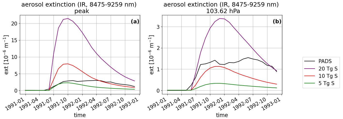
Figure 11 Temporal evolution of the aerosol extinction at the profile peak (a) and the cold-point region (b) for the 8475–9259 nm IR waveband.

3.6 Adjusted forcing caused by the SWV increases

In the following, the adjusted SWV forcing is investigated using the one-dimensional model konrad, as described in Sect. 2.2. Figure 12a shows flux anomalies between an unperturbed run and a run perturbed with the increased SWV levels of the 40 Tg S run but without the volcanic aerosols. Although SWV levels are increased within the complete stratospheric column, the main flux changes occur in the tropopause region where the enhancement is largest, the atmosphere denser and the effect of stratospheric water vapor on the radiative forcing strongest (Solomon et al., 2010). In this region, the incoming solar radiation (SWd) is reduced by absorption, while at lower altitudes there is no difference in the shortwave flux. This is caused by the SWV absorbing part of the solar spectrum which, amongst others, tropospheric water vapor completely absorbs at lower altitudes in the unperturbed run. The reflected solar radiation (SWu) at the surface is only changed negligibly since Δ SWd at the surface is also negligible.

Consequently, the SW contribution (SWd–SWu) to the adjusted forcing at the TOA is very small and negative – accounting for a slightly increased scattering due to the SWV. The emitted longwave radiation (LWu) near the surface is unchanged. This is due to our setup: as the surface temperature is fixed in the perturbed run, the surface LWu is fixed as well. The SWV leads to an increase in the tropopause temperatures, following this increase the emitted longwave radiation at the main SWV levels is also increased, as can be seen in the increased downward longwave radiation (LWd). The LWu above the tropopause region is substantially reduced as the SWV acts as a greenhouse gas and traps part of the outgoing radiation. This leads to the characteristic net positive forcing of the greenhouse gas at the TOA. A comparison to the instantaneous forcing (Fig. 12b) shows that the temperature adaptations in the stratosphere significantly amplify the SWV forcing at the TOA. Whereas the atmospheric levels with increased SWV are warmed, stratospheric cooling is found in higher atmospheric levels, reducing the LWu. This effect has to build up though and consequently is more pronounced in the adjusted SWV forcing. If, in addition to the stratosphere, the troposphere was also allowed to adjust, part of this effect may be counterbalanced (Huang et al., 2020).

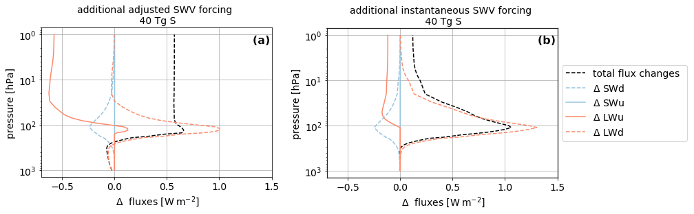
Figure 12 SW and LW contributions to the total adjusted SWV radiative forcing in the tropical stratosphere $[-\mathrm{5},\mathrm{5}]$^∘ latitude for November 1992 of the 40 Tg S eruption. The upward fluxes are in solid lines and positive upward; the downward fluxes are in dashed lines and positive downward. The differences between the perturbed and unperturbed equilibrium states are shown. Panel (a) indicates adjusted forcing and (b) indicates instantaneous forcing.

The temporal evolution of the adjusted inner tropical SWV forcing is shown for all five eruption strengths in Fig. 13. The adjusted forcing caused by the SWV, corresponding to the 2.5 to 10 Tg S run, is below the maximum fluctuations caused by internal variability denoted by the gray line in Fig. 13. The forcing found for these runs could be found for one ensemble member in the 0 Tg case as well, although the time span in which it would occur would most probably be shorter. The adjusted SWV forcing for the 40 Tg S run reaches values of up to 0.65 W m⁻². The signal evolution, especially in the 20 and 40 Tg S cases, matches the evolution already observed for the SWV increases in the tropical region, with two seasonal peaks. However, since SWV at pressures lower than 100 hPa also contributes to the total forcing – although to a smaller extent – and the transport out of the tropical region with the BDC is slow, the first peak forcing times are longer than the peak specific humidity values at 100 hPa in Fig. 4. When considering clouds, the stratospherically adjusted forcing caused by the additional SWV is slightly increased, by 0.1 W m⁻² at most (compare Appendix Fig. E2). As the clouds reflect part of the downgoing SW radiation, some of the SW bands, which could be completely absorbed while traveling through the complete stratosphere and troposphere, are not absorbed entirely. The additional SWV in the stratosphere increases the absorption in these bands and reduces the outgoing SW radiation. This leads to an increase of the forcing.

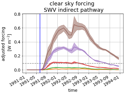
Figure 13 Time evolution of the TOA adjusted clear-sky forcing in the tropical region $[-\mathrm{5},\mathrm{5}]$^∘ latitude for the ensemble mean SWV increases caused by all eruption strengths. The blue line marks the eruption time; the dashed gray line shows the threshold up to which deviations in radiative fluxes can be caused by internal variability. Shaded areas indicate the flux anomaly range originating from the standard deviations of the SWV profiles and are plotted to visualize the signal range.

The monthly SWV forcing does not exhibit a linear behavior with respect to the mass of emitted sulfur or main IR AOD waveband (Figs. A5, A6), as was expected since the monthly cold-point temperatures also did not change in a linear manner with respect to the emitted sulfur mass and the temperature increases showed a hysteretic behavior. However, again, when averaging out the seasonal dependencies and partitioning the time after the eruption in the signal buildup phase (1991, after the eruption), the phase of approximately constant forcing (1992) and the phase of declining signal (1993), the relationship can be fitted to a power function of form aAOD^b+c in the region of interest (Fig. 14). Compared to the cold-point–AOD relation, the signal buildup and relaxation back to the ground state are damped as the transport of the SWV into the stratosphere and out of the tropical region takes place over longer timescales than the cold-point warming or cooling, respectively.

Figure 14 Yearly averages of adjusted forcing due to the additional SWV as a function of AOD (IR, 8475–9259 nm) for the 3 examined years (1991–1993). A power function fit for each year with a corresponding equation is shown.

As the SWV forcing counteracts the volcanic forcing, its relation to the aerosol forcing is of interest. Figure 15a shows the tropical aerosol forcing as calculated using the double radiation call in MPI-ESM. For the evaluation of the forcing in the double radiation call, different conventions exist as far as the evaluations at the TOA or the tropopause are concerned (e.g., compare Forster et al., 2016). As the double radiation call is used to determine an instantaneous forcing, the readout at the tropopause level would be following the standard convention as defined by Hansen et al. (2005) or in the Intergovernmental Panel on Climate Change. However, we present both values for the entire and inner tropics to allow for an easy comparison to other studies. The relative magnitude of the adjusted SWV forcing with respect to the aerosol forcing increases approximately linearly until September 1992 and then reaches a constant values of around 2.5 % for the readout at the tropopause and 4 % percent for the readout at the TOA (Fig. 15b).

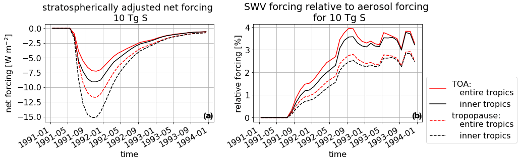
Figure 15 (a) Time evolution of the tropical aerosol forcing for the 10 Tg S run as calculated using the double radiation call in MPI-ESM. The forcing is evaluated for the inner and entire tropics at the tropopause and the TOA. (b) Time evolution of the percentage of aerosol forcing counterbalanced by the SWV forcing in the inner and entire tropics.

4 Discussion

4.1 Magnitude of SWV increases due to indirect volcanic mechanism

In general, the annual cycle of the tropical tropopause temperatures accounts for a variation of the SWV content of ±1.4 ppmv around the mean background at 110 hPa in SAGE II data of the early 1990s (Mote et al., 1996) and ±1.0–1.3 ppmv based on the SPARC Data Initiative multi-instrument mean (SDI MIM) at 100 hPa in 2005–2010 (Davis et al., 2017). In MPI-GE, the variation in the SWV tape recorder signal at the same height reaches up to ±1.1 ppmv. This is in accordance with the SDI MIM and only slightly lower than the SAGE II data. The slightly higher values reported for early 1990 fall into the era of the Mt. Pinatubo eruption, however, and may be increased compared to the multiyear mean due to an amplification of the seasonal signal by the presence of the aerosol layer. This effect led to maximum deviations of up to ±1.6 ppmv in the 10 Tg S scenario of the EVAens simulations. In the case of volcanic perturbations, the alterations in SWV content caused by the indirect temperature controlled entry mechanism via tropopause warming after volcanic eruptions can surpass the SWV variations due to the annual cycle. In our simulations, deviations of more than ±1.1 ppmv are produced in the simulations for emissions equal to or larger than a 10 Tg S eruption, which is an upper bound of the emission estimate for the Mt. Pinatubo eruption (Timmreck et al., 2018). The SWV anomaly caused by the 2.5 Tg S eruption is comparable to changes caused by the quasi-biennial oscillation (QBO), which are [0.16–0.32] ppmv according to the regression analysis by Dessler et al. (2013), whereas the 10 Tg S has an impact stronger than the changes in the BDC (maximum 0.65 ppmv). In climate change studies, the stratospheric water vapor is also affected by doubled CO₂ concentrations. The sea surface temperature (SST) increase leads to a consequent atmospheric humidity increase, amounting up to 6 %–10 % in the stratosphere, with values exceeding 10 % in the lower stratosphere (Wang et al., 2020). These changes of SWV due to increased CO₂ levels are comparable to increases caused by the smaller eruptions of 2.5 and 5 Tg S. However, the SWV changes due to volcanic eruptions are only temporary.

4.2 Comparison to studies based on observations and reanalysis data

While our model study has the advantage that the large ensemble size allows determining the statistical significance of SWV increases and the spread of responses to a volcanic eruption due to internal variability of the Earth system, a model study is always limited by the ability of the model to represent the Earth system realistically. Individual models may differ in the parameterization of convection, the entry of water vapor into the stratosphere and tropopause height. The aerosol profiles used in this study are artificial in the case of EVAens and will include uncertainties of the retrieval in the case of the PADS data set. As our results are therefore at first only representative of the model used in our study, a comparison to results based on or derived from observational evidence of SWV changes after volcanic eruptions is desirable.

During the Mt. Pinatubo period, observations of SWV are scarce, especially as solar occultation measurements by the Halogen Occultation Experiment (HALOE) and SAGE II suffered from aerosol interference in this time period. Therefore, the data usage is discouraged (e.g., Fueglistaler et al., 2013). Although Fueglistaler et al. (2013) mention “anomalously large anomalies” of SWV values shortly after the Mt. Pinatubo eruption in SAGE II data, they also warn that the measurements may be biased by aerosol artifacts since the SWV signal is not present in the HALOE data. However, in the Boulder balloon data, a 1-2 ppmv increase of SWV at 24–26 and 18–20 km levels is registered for 1992 (Oltmans et al., 2000). Most likely due to additional contribution from, e.g., methane oxidation or ENSO signals, the maximum increase is slightly larger than the 1.0–1.2 ppmv shown for the tropical region in Fig. 7 or the value of approximately 0.5 ppmv at 70 hPa at corresponding latitude (compare Appendix Fig. F1). Santer et al. (2003) discuss a global warming of the lower stratosphere caused by the eruption of Mt. Pinatubo amounting to 0.75–1.5 K as measured by MSU. Angell (1997) reports the stratospheric warming due the eruption of Mt. Pinatubo based on radiosonde data. The warmest seasonal anomaly in the 100–50 hPa layer at the Equator reached (2.0 ± 0.8) K, where we find 1.8 K for the 5 Tg S and 5.2 K for the 10 Tg S scenario in October–November–December (OND) 1991. The corresponding SWV increase at background levels of 4.5–5 ppmv can be estimated to be 1.13–1.3 ppmv based on a 12 % increase of SWV per Kelvin. These values are consistent with our findings (Fig. 7). As more regression analyses exist based on reanalysis data, we now compare our results not directly to observations but to the outcome of two regression analysis studies of SWV entry fed by the reanalysis input by Dessler et al. (2014) and Tao et al. (2019). Dessler et al. (2014) studied the different contributors to SWV entry at 82 hPa slightly above the tropical tropopause in their model by using a regression analysis on data output from a trajectory model fed by Modern-Era Retrospective analysis for Research and Applications (MERRA) reanalysis input (Rienecker et al., 2011). They found a maximum increase of 0.34 ppmv in the residual, which partially overlapped the AOD increase caused by the Mt. Pinatubo eruption. This value is lower than our finding of up to (0.8–1.1) ppmv increase in the first and second post-eruption years. Our higher value may be explained by the different quantification approaches: whereas Dessler et al. (2014) indirectly quantified the SWV increase due to Mt. Pinatubo in the residuals after subtracting contributing terms like the BDC, we directly quantified the additional SWV entry by taking the difference between the MPI-GE historical ensemble with volcanic aerosol and the EVAens control run. This allowed us to avoid the subtraction of SWV entry caused by the volcanic eruption but attributed to other sources. For example, in the Dessler et al. (2014) study, the BDC term is described by the heating in the 82 hPa region, but part of this may be caused by the presence of the volcanic aerosol layer. Our method also eliminates other sources of SWV that may have caused the SWV increase prior to the Mt. Pinatubo eruption in the residual of Dessler et al. (2014). Additionally, the tropopause in our historical simulation is located at pressures larger than 100 hPa. Dessler et al. (2014) report that 82 hPa is slightly above the tropopause. Their possibly higher-lying tropopause may also explain part of the difference. Tao et al. (2019) use MERRA-2 (Gelaro et al., 2017), the Japanese 55-year Reanalysis (JRA-55) (Kobayashi et al., 2015) and ERA-Interim (Dee et al., 2011) reanalysis data for the Mt. Pinatubo eruption in their trajectory model. The SWV increase attributed to the volcanic eruption ranges between 0.4 ppmv (ERA-Interim) and 0.8 ppmv (MERRA-2 and JRA-55). Only MERRA-2 explicitly accounts for the volcanic aerosol (Fujiwara et al., 2017): their corresponding 0.8 ppmv SWV increase is in good agreement with the SWV increases found in the first post-eruption year in our historical simulations, although our SWV increase in the second post-eruption year of 1.1 ppmv is larger. As analyzed in Sect. 3.5, this higher increase is mainly caused by the height of the aerosol layer with respect to the cold point. Since the aerosol profiles are imported on fixed pressure levels, without prescribing the distance between the tropopause and the aerosol layer, and the tropopause heights differ amongst various models, the comparison between different studies and models would be facilitated if not only the total volcanic forcing but also the heating in the region were reported when quantifying and comparing volcanically induced SWV increases. A tropopause located at larger pressure in the second post-eruption summer in the reanalysis data could explain the differences between the maximum values of 0.8 ppmv by Tao et al. (2019) using the MERRA-2 reanalysis and our results amounting up to 1.1 ppmv in the second post-eruption summer, as it would lead to a lower heating rate in the cold-point region and consequently a reduced water vapor entry compared to the control years. Additionally, our model does not include interactive chemistry–H₂O sinks could reduce the amount of water vapor and especially the buildup in the second post-eruption summer. However, Löffler et al. (2016) also found a stronger SWV increase in the second post-eruption summer when investigating the perturbations of stratospheric water vapor using nudged chemistry–climate model simulations with prescribed aerosol for the Mt. Pinatubo eruption. The SWV increases for the Mt. Pinatubo eruption reach values of up to 35 % compared to the unperturbed run in the inner tropical average. Thus, our finding of an increase of 25 % above the unperturbed levels for the historical simulations (compare Fig. B1) lies between the estimates from reanalysis data by Tao et al. (2019) and the chemistry–climate studies by Löffler et al. (2016). In EVAens, where the temporal evolution of the extinction profile does not lead to as drastic changes in the vertical shape as in the PADS forcing data set, the temporal evolution of the increase in SWV is similar to the evolution found by Tao et al. (2019), with only one prominent maximum. Maximum values of SWV increase are in the range of 0.3 and 1.1 ppmv for the 5 and 10 Tg S EVAens runs – covering the estimated sulfur emission range of Mt. Pinatubo and in agreement with Tao et al. (2019).

4.3 SWV contributions due to the indirect volcanic and direct volcanic injection

Unlike the direct volcanic mechanism, the indirect volcanic pathway is active for the entire lifetime of the volcanic aerosol in the lower stratosphere, whereas the direct volcanic injection is a singular event. There is no study known to us comparing the SWV entry due to both events within one framework. Although up to 80 % of the eruption volume can be water vapor (Coffey, 1996), rapid condensation can remove 80 %–90 % of this humidity on the way to the stratosphere (Glaze et al., 1997). There are only a few cases of direct volcanic injections reported, which cover relatively small eruption events. The water vapor within the eruption column reaching the stratosphere did not lead to elevated SWV above background for more than a week locally in the few cases reported, i.e., the eruption of Kasatochi (in 2008) with maximum SWV content of 9 ppmv (Schwartz et al., 2013) lasting for around 1 d, the eruption of Calbuco (2015) with 10 ppmv values for approximately a week (Sioris et al., 2016a) and the eruption of Mt. St. Helens with (64 ± 4) ppmv (Murcray et al., 1981) detectable above background for around a week but only on a local and not a global scale. In the case of the Mt. Pinatubo eruption, the model estimates for the direct volcanic injection tended to have a larger range and maximum values than the estimates based on observational data (Joshi and Jones, 2009). In contrast, the indirect volcanic pathway allows for slower but more continuous, raised stratospheric water vapor levels ultimately spreading throughout the globe but with lower peak values. These enhanced SWV levels are detectable in our ensemble mean even years after the actual volcanic eruption if the emitted sulfur amount is larger than 10 Tg S. Depending on the explosivity of the volcano, the relative contributions of the direct and indirect volcanic injection mechanisms to SWV increases should change: for small eruptions, the direct volcanic injection will lead to a relatively high increase in SWV, which is short lived and spatially confined. For the larger eruptions, this short-lived SWV enhancement is followed by a relatively stable increase of SWV which spreads throughout the entire globe, dominating the SWV increase due to the volcanic eruption.

4.4 SWV forcing

In our simulations, the stratospherically adjusted forcing caused by the increase of SWV in the tropical region amounts to maximally 2.5 % to 4 % of the tropical aerosol forcing over the time frame for the 10 Tg S eruption. However, although a decline of the tropical forcing within the 3-year time frame is found, the forcing around the complete globe will last longer than the impact of the volcanic aerosols. The decline in tropical stratospheric water vapor is caused by its transport to the poles by the BDC, leading to a regional shift of the location of the SWV forcing (see Fig. F1). Forster and Shine (2002) found the polar SWV forcing to be 2.5 times stronger than the tropical forcing: since in the polar region the tropopause height is lower and the water vapor content is generally lower, SWV increases of the same magnitude have a much larger impact there than in the tropical region. Based on the factor of 2.5, the 40 Tg S run 1993 values would cause an adjusted forcing of up to 0.5 W m⁻² in the polar region, whereas the aerosol forcing is back to the levels of the 2.5 Tg S run by 1993. This shift in relative magnitude is one of the factors contributing to the positive TOA imbalance at the end of 1993 (for 20 and 40 Tg S in Fig. 2).

For the eruption of Mt. Pinatubo, with (7.5 ± 2.5) Tg S emitted, earlier estimates of SWV forcing exist. Joshi and Shine (2003) calculated the global SWV forcing to be 0.1 W m⁻². Our 10 Tg S adjusted forcing results of up to 0.11 W m⁻² are nearer to the estimate by Joshi and Shine (2003) than our 5 Tg S results of up to 0.03 W m⁻². In 1992, the adjusted forcing in the inner tropics lies between [0.02–0.03] W m⁻² for the 5 Tg S and [0.06–0.11] W m⁻² for the 10 Tg S scenarios. The better agreement of our 10 Tg S adjusted SWV forcing with Joshi and Shine (2003) value for the Mt. Pinatubo SWV forcing can be attributed to two points: first, the form and location of the forcing profile with respect to the cold point is crucial when comparing model results of increased SWV levels and the consequent changes in SWV forcing (s. Sect. 3.5). This may contribute to differences between our values and the ones in the Joshi and Shine (2003) analysis. Second, the polar forcing will be stronger than the tropical forcing which was calculated with konrad. Using the ratio of polar forcing to tropical forcing by Forster and Shine (2002), the polar estimate would be [0.05–0.08] W m⁻² for 5 Tg S and [0.15–0.28] W m⁻² for 10 Tg S.

In their study on direct volcanic SWV entry for the Krakatau eruption, Joshi and Jones (2009) found a LW forcing of + (0.33 ± 0.09) W m⁻² for a direct volcanic entry above 100 hPa of 1.5 ppmv using the downward TOA heat flux, climate feedback parameter and near-surface temperature changes. They chose a relatively high estimate of SWV increase, which would approximately correspond to the SWV increases in our 20 Tg S eruption run. As the TOA-SW contribution to our forcing is negligible (see Fig. 12), a comparison to our total forcing is possible. The corresponding value of [0.21–0.33] W m⁻² is in the lower part of the range found by Joshi and Jones (2009), which is likely caused mainly by the restriction of our study to the tropical region.

Krishnamohan et al. (2019) also mentioned the contribution of aerosol induced SWV changes to the flux changes at the TOA in a geoengineering study; however, they did not explicitly calculate it. The amount of shortwave forcing they attribute to additional SWV is much higher than our value and also positive. Presumably these differences are caused by the forcing including tropospheric adjustments and using CO₂ concentrations equal to twice the amount of their pre-industrial control run and thus cannot be compared to our study.

In order to put the adjusted radiative SWV forcing due to the indirect volcanic pathway into a broader context, we compare it with SWV forcing due to anthropogenic CO₂ and methane releases: the rate of radiative forcing increase due to CO₂ in the 2000s² reached values of almost 0.03 $\mathrm{W}{\mathrm{m}}^{-\mathrm{2}}{\mathrm{yr}}^{-\mathrm{1}}$ and a total of (1.82 ± 0.19) W m⁻² for the 1750 to 2011 time frame, whereas the additional radiative forcing due to methane in the same time frame is (0.48 ± 0.05) W m⁻² (Myhre et al., 2013)³. The forcing caused by the SWV entering the stratosphere via the indirect volcanic entry mechanism exceeds the yearly increase of forcing due to CO₂ in the 2000s starting with the 5 Tg S run. The peak adjusted tropical SWV forcing for the 40 Tg S scenario amounts to one-third of the total CO₂ forcing (due to the accumulated emissions from 1750 to 2011) and is larger than the forcing due to methane emissions for the same period.

4.5 Predictability of responses

The increases in cold-point temperature and SWV are delayed events. Time is required for it to build up the signals as the aerosols warm the cold-point region, allowing more water vapor transit into the stratosphere. An approximately stable phase with fluctuations due to the seasonal cycle is attained a couple of months after eruption. The cold-point warming has stabilized. The SWV forcing is mainly determined by the additional SWV entering the stratosphere each month as the tropopause region is the region in which WV has the strongest radiative effect. The corresponding buildup of tropical SWV forcing due to an accumulation of SWV in the stratosphere is therefore counteracted by the transport to higher altitudes and to the polar region by the BDC. Due to the transient character of the processes – the buildup of the forcing and the consequent decline as well as the time shift between effect and response – our analysis showed that a linear relationship between AOD and cold-point warming, or SWV, cannot be determined for the entire era after the volcanic eruption. Time phases have to be considered as well to account for the resulting hysteresis. Other parameters additionally constrain the cold-point warming and SWV response. The season during which the eruption occurs will influence the impact of the aerosols: the CP warming will be most effective during the peak times of the tape recorder signal around September. Each volcanic eruption is different and parameters like the eruption location, amount of emitted sulfur and specifically the location of the aerosol layer will have a massive influence both on cold-point warming and SWV entry/forcing. Feedbacks like the SWV forcing in the TTL will enhance the CP warming and lead to higher SWV forcing at same AODs eventually before the aerosols fall out. Nevertheless, approximately a power function relationship of form aAOD^b+c can be found in our simulations for CP warming and SWV forcing with respect to IR AOD after the volcanic eruptions when taking yearly averages. These results, however, must be interpreted with care, and the derived formulas are only applicable for tropical eruptions occurring in June and reaching to similar heights in the stratosphere. Generally, the knowledge – both of the respective CP warming in the inner tropics for a specific volcanic eruption and the respective background SWV in the cold-point region – allows for a relatively accurate prediction of the inner tropical increases in SWV levels when using a 12 % SWV increase per Kelvin warming in the mean CP values.

5 Conclusion and outlook

Our study of EVAens and the historical simulations led us to draw the following conclusions:

1. The analysis of the ensemble runs showed the difficulty to extract the volcanic signal in the SWV if only individual observations are available, as internal variability of SWV in the control run could produce SWV values as large as the variation found for some of the 10 Tg S ensemble members in our simulations. Ensemble mean SWV increases are already significant (t test with p=0.05) in the 2.5 Tg S eruption.

2. The increase in stratospheric water vapor does not remain constant throughout year but can vary with the seasons. An amplification of the seasonal cycle could be observed, especially in the 20 and 40 Tg S scenarios.

3. The average WV at the cold point entering the stratosphere after volcanic eruptions can be approximated with only minor errors using the mean saturation water vapor pressure over ice at the respective average tropical cold-point temperature for all investigated aerosol profiles of EVAens. When given a base value of an unperturbed atmospheric state, a 12 % SWV increase per Kelvin increase in cold-point temperature is a good first estimate for eruption strengths up to 40 Tg S.

4. The comparison of the idealized EVAens simulations and MPI-GE historical simulations of Mt. Pinatubo show that neither the simulated TOA radiative imbalance nor the estimated amount of emitted stratospheric sulfur suffice to constrain the SWV increases. However, the aerosol layer shape and height with respect to the tropopause play a crucial and dominating role when estimating the SWV increases.

5. The adjusted tropical forcing caused by the additional SWV lasts longer than the forcing caused by the aerosol layer itself, and its contribution to the total volcanic forcing grows with time as the aerosols fall out. For the 20 and the 40 Tg S scenarios, the TOA radiative imbalance shows a positive value by the end of the simulation. Part of this positive TOA radiative imbalance can be attributed to the forcing by the additional SWV.

6. When considering also the time dependence, a power function relationship of form aAOD^b+c between yearly averaged tropical cold-point warming/adjusted SWV forcing and IR AOD can be deduced. This relationship however only holds for comparable eruptions occurring at the same time of the year in the tropics. Additionally, the final eruption height and aerosol profile shape have to match the ones used within our framework.

Based on our study, follow-up questions for future investigations arise. Our study only focuses on the indirect temperature controlled injection and, although other studies focus on the direct injection, no study known to us combines both effects allowing for a direct comparison within a single framework. Using integrated plume models for a combined study would allow the quantification of the entire SWV changes and for an estimation of their relative importance. As we use no interactive chemistry, the H₂O value determined by us might be overestimating the SWV from the indirect volcanic injection remaining in the stratosphere. A study using interactive chemistry would allow the assessment of the impact of H₂O sinks on the volcanically induced SWV increase and ozone chemistry. Of particular interest is the impact of the additional H₂O on the oxidation process of SO₂, as well as on sulfate particle formation and growth. A follow-up study on this topic could give a lower boundary estimate for the SWV increases and the changed aerosol lifetime (compare Case et al., 2015, Kilian et al., 2020). Additionally, the mechanism of the indirect volcanic injection has implications beyond that of a volcanic eruption: as geoengineering scenarios also apply sulfur derivatives in the stratosphere, an investigation of the long-term SWV signal within these scenarios may be of interest as well (e.g., Boucher et al., 2017).

Appendix A: Scaling of different physical parameters altered by the presence of volcanic aerosols

Following the discussion in Sect. 3.1, 3.2 and 3.6, the graphs for TOA imbalance (Fig. A1), surface temperature (Fig. A2), cold-point temperature changes (Fig. A3) and SWV forcing (Fig. A5) are shown. Each ensemble mean is divided by the mass of emitted sulfur. In the case of the cold-point temperature changes and the SWV forcing, the dependence of monthly mean values of cold-point temperature change and SWV forcing is shown as a function of AOD in the IR waveband of [8475, 9259] nm in Figs. A4 and A6.

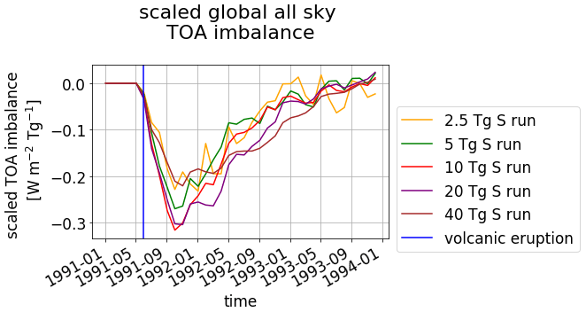
Figure A1 Scaled TOA imbalance for the five volcanically perturbed EVAens runs (2.5, 5, 10, 20 and 40 Tg S). The ensemble means are shown. The vertical blue line marks the eruption time. All TOA imbalances are divided by the mass of emitted sulfur.

Figure A2 Scaled surface temperature for the five volcanically perturbed EVAens runs (2.5, 5, 10, 20 and 40 Tg S). The ensemble means are shown. The vertical blue line marks the eruption time. All surface temperatures are divided by the mass of emitted sulfur.

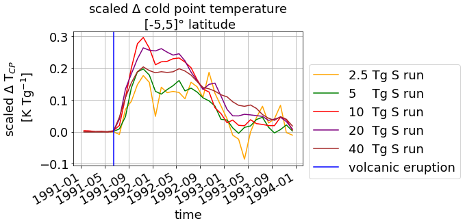
Figure A3 Scaled temporal evolution of the mean CP temperature anomaly. The time of the volcanic eruption is indicated by a vertical blue line. All changes in cold-point temperature are divided by the mass of emitted sulfur.

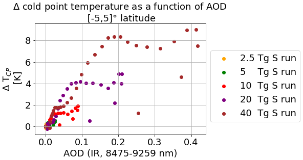
Figure A4 Scatter plot of AOD in the IR waveband (8475–9250 nm) and CP temperature anomaly for all time steps in the first 2.5 years after the eruption.

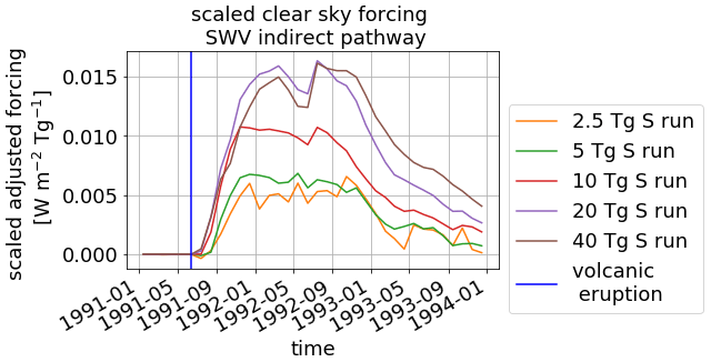
Figure A5 Scaled time evolution of the adjusted clear-sky SW forcing in the tropical region $[-\mathrm{5},\mathrm{5}]$^∘ latitude for all eruption strengths. The blue line marks the eruption time. All clear-sky forcings are divided by the mass of emitted sulfur. Incoming fluxes are defined as positive; outgoing fluxes are defined as negative.

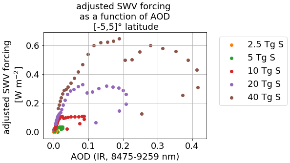
Figure A6 Scatter plot of AOD in the IR waveband (8475–9250 nm) and the clear-sky SWV forcing for all time steps in the first 2.5 years after the eruption.

Appendix B: Percental changes in the tape recorder signal

Complementary to the plot in Sect. 3.3, we show the differences in water vapor between perturbed and unperturbed states with respect to the unperturbed state in percent.

Figure B1 Percental difference in water vapor above 140 hPa in the tropical average over $[-\mathrm{23},\mathrm{23}]$^∘ latitude for the pure sulfur injections of EVAens (2.5, 5, 10, 20 and 40 Tg S). The lowermost panel shows the MPI-GE historical simulations for Mt. Pinatubo using the PADS forcing data set. The height of the WMO tropopause is indicated by a black line; the cold-point pressure is indicated by a dashed black line. In regions not covered by black crosses, statistically significant differences between stratospheric water vapor values of the perturbed and unperturbed runs (t test at p=0.05) were found.

Appendix C: Intra-ensemble variability in the entire tropics

Here, we show the complementary plots to those in Sect. 3.4 for the intra-ensemble variability in the entire tropics ($[-\mathrm{23},\mathrm{23}]$^∘ latitude).

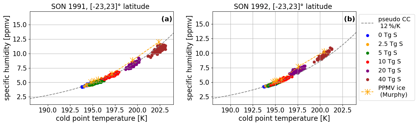
Figure C1 Seasonal averages of specific humidity at cold point as a function of cold-point temperature for SON 1991 (a) and 1992 (b) accounting for the entire tropics. Values for each individual ensemble member are shown as dots for the entire tropics. An approximation (see text) for the Clausius–Clapeyron equation at this temperature range with an 12 % increase of specific humidity per Kelvin is indicated by a dashed gray line. The exact solution for the Clausius–Clapeyron equation over ice by Murphy and Koop (2005) is calculated for the average ensemble cold-point temperatures and pressure and shown in orange.

Appendix D: Aerosol extinction profiles – 550 nm solar waveband

Complementary to the discussion on the infrared extinction profiles in Sect. 3.5, the 550 nm solar waveband is shown in the following plots.

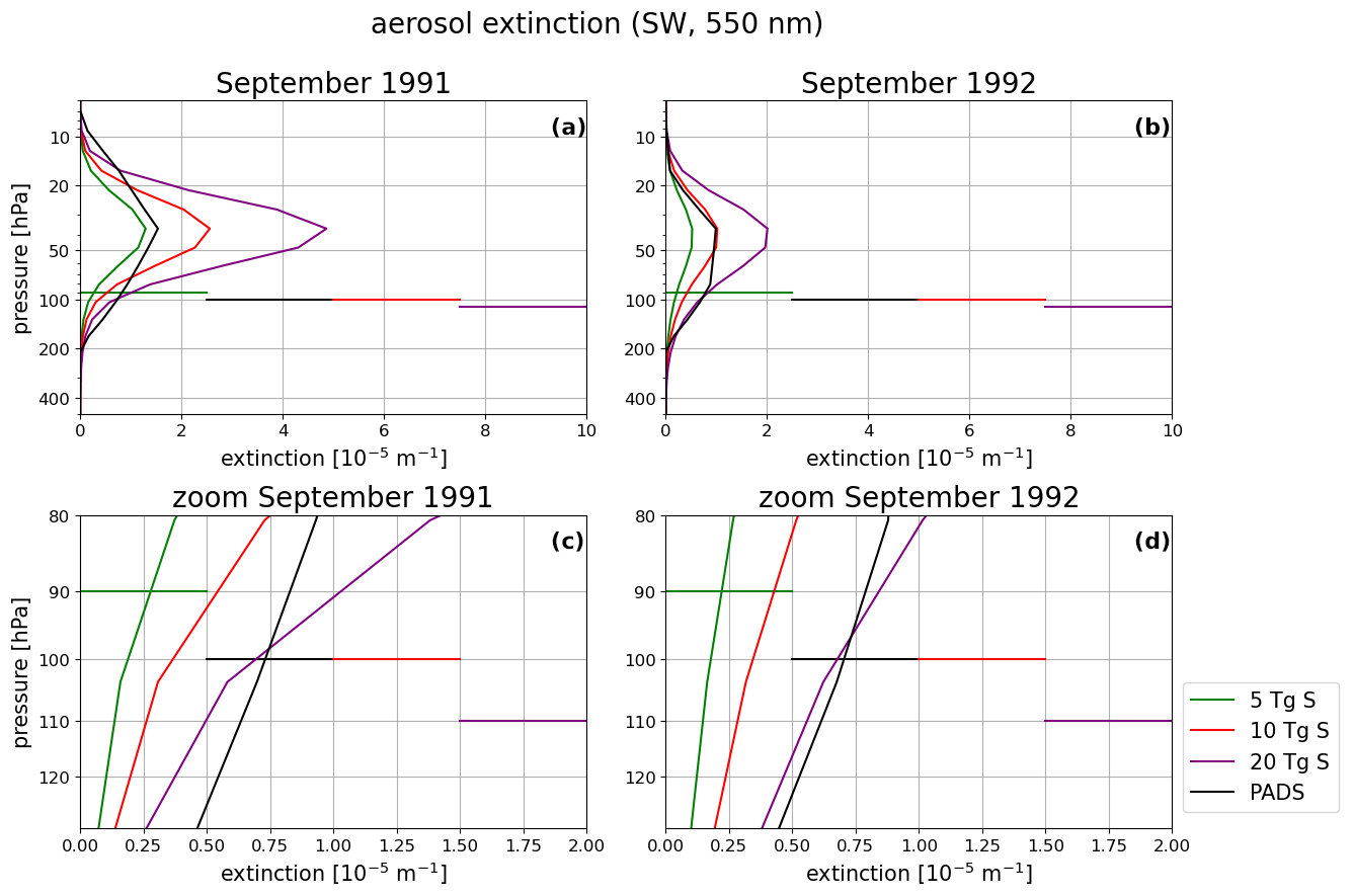
Figure D1 Tropical average of the aerosol extinction profile in the 550 nm solar waveband for the EVA forcing corresponding to 5, 10 and 20 Tg S as well as the PADS forcing for the Mt. Pinatubo eruption.

Appendix E: SWV forcing – SW component

Figure E1 shows the very small contribution of the SW component to the total adjusted SWV forcing presented in Sect. 3.6.

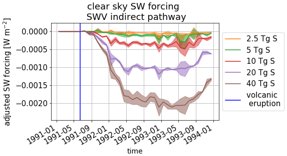
Figure E1 Time evolution of the SW component to the adjusted clear-sky forcing in the tropical region at $[-\mathrm{5},\mathrm{5}]$^∘ latitude for the ensemble mean SWV increases caused by all eruption strengths. The blue line marks the eruption time. The flux range originating from the standard deviations of the SWV profiles is plotted to visualize the signal range.

The total forcing and its SW component for the cloudy-sky case as discussed in Sect. 3.6 is shown in Fig. E2.

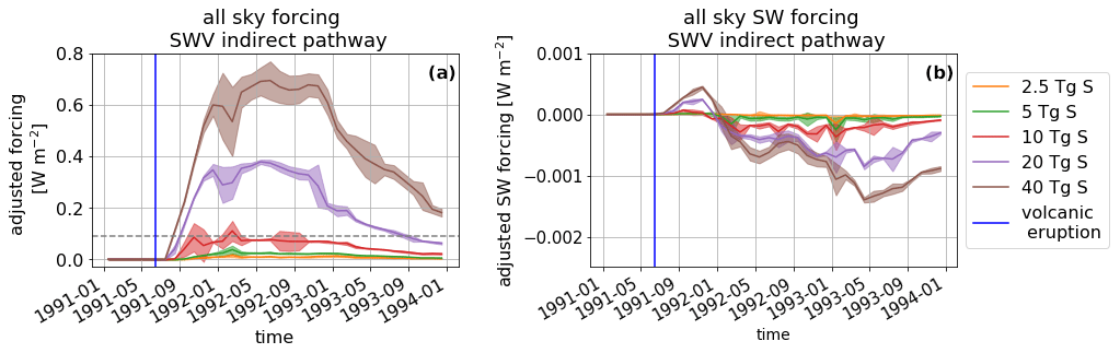
Figure E2 Time evolution of the (a) total and (b) SW component to the adjusted all-sky forcing in the tropical region at $[-\mathrm{5},\mathrm{5}]$^∘ latitude for the ensemble mean SWV increases caused by all eruption strengths. The blue line marks the eruption time. The flux range originating from the standard deviations of the SWV profiles is plotted to visualize the signal range.

Appendix F: Global spread of the stratospheric water vapor

Figure F1 shows the spread of the additional SWV around the globe as mentioned in the Discussion (Sect. 4.4).

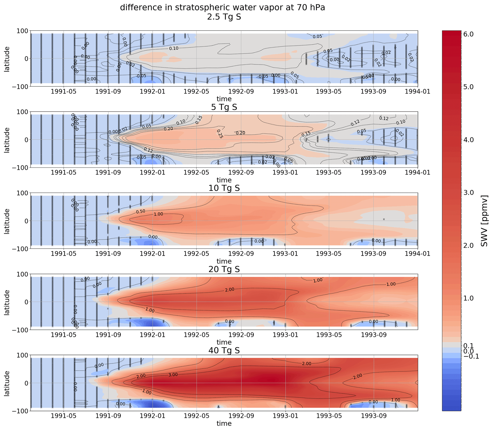
Figure F1 Difference in stratospheric water vapor content at 70 hPa as a function of time and latitude. Black crosses mark the regions of statistical significance of the data (Mann–Whitney U test at p=0.05).