Case study of a humidity layer above Arctic stratocumulus and potential turbulent coupling with the cloud top

Specific humidity inversions (SHIs) above low-level cloud layers have been frequently observed in the Arctic. The formation of these SHIs is usually associated with large-scale advection of humid air masses. However, the potential coupling of SHIs with cloud layers by turbulent processes is not fully understood. In this study, we analyze a 3 d period of a persistent layer of increased specific humidity above a stratocumulus cloud observed during an Arctic field campaign in June 2017. The tethered balloon system BELUGA (Balloon-bornE moduLar Utility for profilinG the lower Atmosphere) recorded vertical profile data of meteorological, turbulence, and radiation parameters in the atmospheric boundary layer. An in-depth discussion of the problems associated with humidity measurements in cloudy environments leads to the conclusion that the observed SHIs do not result from measurement artifacts. We analyze two different scenarios for the SHI in relation to the cloud top capped by a temperature inversion: (i) the SHI coincides with the cloud top, and (ii) the SHI is vertically separated from the lowered cloud top. In the first case, the SHI and the cloud layer are coupled by turbulence that extends over the cloud top and connects the two layers by turbulent mixing. Several profiles reveal downward virtual sensible and latent heat fluxes at the cloud top, indicating entrainment of humid air supplied by the SHI into the cloud layer. For the second case, a downward moisture transport at the base of the SHI and an upward moisture flux at the cloud top is observed. Therefore, the area between the cloud top and SHI is supplied with moisture from both sides. Finally, large-eddy simulations (LESs) complement the observations by modeling a case of the first scenario. The simulations reproduce the observed downward turbulent fluxes of heat and moisture at the cloud top. The LES realizations suggest that in the presence of a SHI, the cloud layer remains thicker and the temperature inversion height is elevated.

1 Introduction

The Arctic atmospheric boundary layer (ABL) exhibits numerous particular features compared to lower latitudes, such as persistent mixed-phase clouds, multiple cloud layers decoupled from the surface, and ubiquitous temperature inversions close to the surface. Local ABL and cloud processes are complex and not completely understood, but they are considered an important component to explain the rapid warming of the Arctic region (Wendisch et al., 2019). One of the special features frequently observed in the Arctic are specific humidity inversions (SHIs), although specific humidity is generally expected to decrease with height (Nicholls and Leighton, 1986; Wood, 2012). The relative frequency of occurrence of low-level SHIs in summer is estimated to be in the range of 70 %–90 % over the Arctic ocean (Naakka et al., 2018).

Arctic SHIs have been observed during past field campaigns (Sedlar et al., 2012; Pleavin, 2013), e.g., the Surface Heat Budget of the Arctic Ocean (SHEBA;  Uttal et al., 2002) in 1997–1998, or the Arctic Summer Cloud Ocean Study (ASCOS;  Tjernström et al., 2014) in 2008. Furthermore, a number of studies on the climatology of SHIs have been published (e.g.,  Naakka et al., 2018; Brunke et al., 2015; Devasthale et al., 2011). SHIs occur most frequently over the Arctic ocean and are strongest in summer. In the lower troposphere, they often occur in conjunction with temperature inversions and high relative humidity but are also linked to the surface energy budget (Naakka et al., 2018). Formation processes and interactions of SHIs with clouds have been investigated in large-eddy simulations (LESs). For example, Solomon et al. (2014) showed that a specific humidity layer becomes important as a moisture source for the cloud when moisture supply from the surface is limited. Pleavin (2013) studied how the SHIs support the mixed-phase clouds to extend into the temperature and humidity inversion.

Mostly, the formation of the summertime SHIs is attributed to large-scale advection of humid air masses. In the Arctic, especially over sea ice, moisture advection is the critical factor for cloud formation and development (Sotiropoulou et al., 2018). SHIs form when warm, moist air is advected over the cold sea ice surface and moisture is removed through condensation and precipitation from the lowest ABL part. This and further simplified formation processes are discussed by Naakka et al. (2018).

SHIs can contribute to the longevity of Arctic mixed-phase clouds (Morrison et al., 2012; Sedlar and Tjernström, 2009), which dominate the near-surface radiation heat budget in the Arctic (Intrieri et al., 2002). When a SHI is located closely above an Arctic stratocumulus, it can provide moisture that may drive the cloud evolution due to cloud top entrainment. In contrast, in the typical marine sub-tropical or mid-latitude cloud-topped ABL, dry air from above is entrained into the cloud (Albrecht et al., 1985; Nicholls and Leighton, 1986; Katzwinkel et al., 2012). However, SHIs are not well represented in global atmospheric models, where the SHI strength is typically underestimated (Naakka et al., 2018), or the SHIs are not reproduced (Sotiropoulou et al., 2016).

Previous studies on SHIs have been based on radiosoundings, remote sensing observations, reanalysis data, or LESs. Most observational studies rely on profiles of mean thermodynamic parameters from radiosoundings, which might be influenced by sensor wetting after cloud penetration in the SHI region. A systematic bias in radiosonde humidity measurements due to sensor wetting or other error sources is a serious concern when studying SHIs, particularly under moist and cold conditions. To exclude systematic biases, one aim of this work is to carefully assess the validity of the SHI observations. Due to the limited time resolution of radiosondes, those measurements do not allow for turbulence observations to analyze the exchange processes between the SHI and cloud top. To date, very few data are available to characterize and quantify the turbulent and radiative energy fluxes at SHIs. However, in particular the vertical turbulent exchange of mass and energy is necessary to understand the importance of SHIs for cloud evolution and lifetime.

To investigate the exchange processes between the cloud layer and the SHI, we performed tethered balloon-borne high-resolution vertical profile measurements of turbulence and radiation during a 3 d period in the framework of the campaign Physical Feedbacks of Arctic Boundary Layer, Sea Ice, Cloud and Aerosol (PASCAL) (Wendisch et al., 2019). The observations are supplemented by LES for the same period. We focus on a detailed case study with a persistent SHI above a stratocumulus deck to answer the following research question: how are the SHI and the cloud top connected by turbulent mixing?

The paper is structured as follows: Sect. 2 describes the observations. In Sect. 3, we discuss humidity measurements in cloudy and cold conditions and potential error sources. For the case study, Sect. 4 analyzes the vertical ABL structure around the SHI and the relation of SHI, cloud top, and temperature inversion. In Sect. 5, we investigate the turbulent coupling between SHI and the cloud layer, and the turbulent transport of heat and moisture. We close with a discussion of the impact of the SHI on the cloud by means of LES in Sect. 6.

2 Observations

2.1 The PASCAL expedition

The observations analyzed in this study were performed during PASCAL (Wendisch et al., 2019), which took place in the sea-ice-covered area north of Svalbard in summer 2017. The RV Polarstern (Knust, 2017) carried a suite of remote sensing and in situ instrumentation. Additionally, an ice floe camp was erected in the vicinity of the ship (Macke and Flores, 2018). Knudsen et al. (2018) describe the synoptic situation during the operation of the ice floe camp as climatologically warm with prevailing warm and moist maritime air masses advected from the south and east. The meteorological conditions were influenced by a high-pressure ridge east of Svalbard. The present study is based on measurements with instruments carried by the tethered balloon system BELUGA (Balloon-bornE moduLar Utility for profilinG the lower Atmosphere;  Egerer et al., 2019a). BELUGA was launched from the sea ice floe at around 82^∘ N, 10^∘ E in the period of 5–14 June 2017. The balloon measurements are complemented by radiosoundings launched every 6 h (Schmithüsen, 2017) and by ship-based remote sensing observations from a vertical-pointing, motion-stabilized cloud radar (Griesche et al., 2020c), a lidar (Griesche et al., 2020b), and a microwave radiometer of the OCEANET platform (Griesche et al., 2020d), which were processed with the synergistic instrument algorithm Cloudnet (Griesche et al., 2020a).

Figure 1 Temporal development of the specific humidity vertical profile observed by radiosondes. The radar-retrieved cloud top height is depicted as a black line; the cloud base height derived from the lidar near-field channel is indicated as a grey line. The red lines represent the BELUGA flight profiles.

2.2 Observation period

The observational basis for this study is a persistent layer of increased specific humidity above a single-layer stratocumulus deck during the period between 5 and 7 June 2017. Figure 1 illustrates the temporal development of the vertical specific humidity profile derived from radiosonde measurements. Cloud top and bottom and the time–height curves of the corresponding BELUGA flights are added for the investigated period. The BELUGA flights were conducted around noon on each of the three consecutive days. A local maximum of specific humidity is observed above the cloud top throughout almost the entire period, with a slight diurnal cycle peaking at noon and a maximum specific humidity on 6 June. It is worth noting that the observations show a well-defined layer of increased specific humidity, hereafter referred to as the humidity layer, rather than a distinct and sharp SHI with only a slight decrease above.

The cloud top and base height in Fig. 1 are estimated from the cloud radar and lidar (near-field channel) data, averaged over 30 s and with a vertical resolution of 30 m. Throughout the 3 d period, cloud height and thickness decrease to a minimum at noon of 6 June and thereafter increase again. The cloud is almost permanently of mixed-phase type with a maximum liquid water content (LWC) between 0.15 and 0.6 g m⁻³ and an estimated ice water content (IWC) of about 0.03 g m⁻³ derived from Cloudnet data (not shown here).

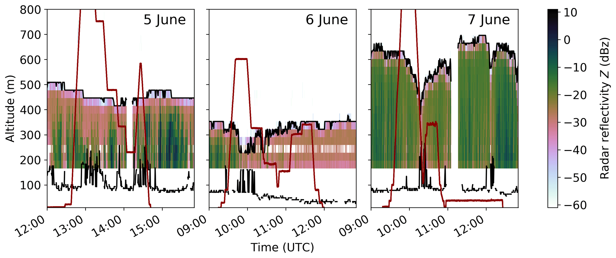
Figure 2 BELUGA flight profiles for 5, 6, and 7 June (red lines) with the radar reflectivity Z and cloud boundaries (black lines, as in Fig. 1).

Figure 1 depicts the high variability in cloud top and bottom heights. To illustrate the cloud situation around the BELUGA flights in more detail, Fig. 2 shows the radar reflectivity and cloud boundaries for the particular three balloon flights. On 5 June, the cloud top height is approximately constant, whereas on 6 June the cloud top fluctuates between 350 and 230 m in the course of the flight. During the 7 June flight, the cloud layer thins by 110 m starting from the cloud top.

2.3 BELUGA setup

The BELUGA system consists of a 90 m³ helium-filled tethered balloon with a modular setup of different instrument packages to explore the ABL between the surface and 1500 m altitude. BELUGA can operate under cloudy and light icing conditions in the Arctic. Fixed to the balloon tether, a fast (50 Hz resolution) ultrasonic anemometer, supported by an inertial navigation system, measures the wind velocity vector in an Earth-fixed coordinate system together with the sonic temperature. Especially at low specific humidity, the sonic temperature is close to the virtual temperature, which will be used in the following. Furthermore, barometric pressure, relative humidity, and the static air temperature are measured with lower resolution (1 Hz). Relative humidity (RH) is measured with a capacitive humidity sensor. The housing of the RH sensor, which has a high diffusivity for water vapor, also accommodates a temperature sensor for the sensor-internal temperature. The air temperature is measured with a PT100 for reference and a thermocouple for temperature fluctuations (at 50 Hz). A second instrument payload is fixed simultaneously to the tether, measuring broadband terrestrial and solar net irradiances. Technical details on BELUGA, its instrumentation, and operation during PASCAL as well as data processing methods are given by Egerer et al. (2019a).

3 Specific humidity measurements in a moist environment

A cold and moist environment poses considerable challenges for the measurement of specific humidity. This can lead to measurement artifacts in the region of the SHI. Therefore, in this section we discuss the measurement of specific humidity with BELUGA and radiosondes as well as possible sources of error and their effects. Specific humidity q is derived from air temperature T and RH using

$$\begin{array}{}\text{(1)}& {\displaystyle }{\displaystyle }q={\displaystyle \frac{R_{\mathrm{d}}/R_{\mathrm{v}}\cdot e_{\mathrm{s}}\left(T\right)\cdot \text{RH}}{p-(\mathrm{1}-R_{\mathrm{d}}/R_{\mathrm{v}})\cdot e_{\mathrm{s}}\left(T\right)\cdot \text{RH}}},\end{array}$$

with the static pressure p, the ratio of specific gas constants of dry air and water vapor $R_{\mathrm{d}}/R_{\mathrm{v}}\approx \mathrm{0.622}$, and the temperature-dependent saturation vapor pressure e_s(T). In this study, the measurements of RH and T are obtained by regular radiosoundings (Vaisala RS92-SGP) and observations with the BELUGA system. Both methods use capacitive RH sensors, suffering from several limitations (Wendisch and Brenguier, 2013).

3.1 Error sources for humidity measurements

Several studies address the associated systematic errors of radiosonde RH and T measurements and identify three main sources, (i) wet-bulbing, (ii) solar heating, and (iii) time response errors:

• i.

  Wet-bulbing occurs when a water film develops on the sensor during cloud penetration, with subsequent evaporative cooling under sub-saturated conditions above the cloud. This effect leads to an overestimation of RH and underestimation of T in the sub-saturated environment until the water film has completely evaporated. Jensen et al. (2016) show that wet-bulbing is an issue for the radiosonde type used during PASCAL. However, the error induced by wet-bulbing is difficult to quantify (Dirksen et al., 2014).

• ii.

  Exposure of an RH sensor to direct sunlight above a cloud causes a radiation dry bias (measured RH is too low) of up to 5 % in the lower troposphere (Miloshevich et al., 2009; Wang et al., 2013). The error is corrected in the radiosonde data processing algorithm (Jensen et al., 2016). However, this correction is intended for cloud-free conditions. Solar heating also influences temperature measurements (Sun et al., 2013), but the effect on radiosonde temperature is negligible at low altitudes. For BELUGA, the temperature and RH sensors are shielded against direct solar radiation, but the sensor surroundings might warm and influence the measurements.

• iii.

  Furthermore, the time response for RH and T measurements is finite. Compared to the effects (i) and (ii), this part of the sensor behavior can be quantified by the time constant τ. Assuming a first-order sensor response, the time dependence of a measured signal x_m(t) (RH or T in our case) is given by

  $$\begin{array}{}\text{(2)}& {\displaystyle }{\displaystyle \frac{\mathrm{d}{x}_{\mathrm{m}}}{\mathrm{d}t}}=\mathrm{1}/\mathit{\tau }\left(x_{\mathrm{a}}-x_{\mathrm{m}}\right),\end{array}$$

  with the e⁻¹ time constant τ and the ambient (“true”) signal x_a.

  The time-lag-corrected signal is

  $$\begin{array}{}\text{(3)}& {\displaystyle }{\displaystyle }{x}_{\mathit{\tau }}={\displaystyle \frac{{\stackrel{\mathrm{̃}}{x}}_{\mathrm{m}}\left(t\right)-\left[{\stackrel{\mathrm{̃}}{x}}_{\mathrm{m}}(t-\mathrm{\Delta }t)\cdot e^{-\mathrm{\Delta }t/\mathit{\tau }}\right]}{\mathrm{1}-e^{-\mathrm{\Delta }t/\mathit{\tau }}}},\end{array}$$

  with Δt being the time step between two consecutive measurement points (Miloshevich et al., 2004). Here, we assume that the time-corrected value (index τ) is equal to the ambient value x_a. The tilde in Eq. (3) represents the low-pass-filtered, measured time series.

Although radiosonde data processing routines consider the time response error, fast humidity changes in cold conditions are still affected (Smit et al., 2013; Edwards et al., 2014). The time constants for the BELUGA RH sensor were estimated in a laboratory study (see Appendix A) and are τ_RH≈50 s for RH and ${\mathit{\tau }}_{T_{\mathrm{s}}}\approx \mathrm{70}$ s for the internal temperature. The time constant for the T measurements based on the thermocouple on BELUGA was found to be below 1 s (Egerer et al., 2019a) and, thus, has a minor influence on the vertical temperature profile compared to the humidity observations.

3.2 Sensitivity of q to the RH and T profile

We perform sensitivity studies to analyze how the three error sources (cf. Sect. 3.1) for T and RH measurements combine and influence the derivation of q. The errors are simulated as T and RH deviations from a synthetic reference case (grey line in Fig. 3), which represents a simulated measurement of a temperature inversion combined with a decrease in RH. The temperature linearly increases by 6 K in the 200 m thick inversion layer, whereas RH linearly decreases from 100 % to 40 % in the same height range, resulting in monotonically decreasing specific humidity without a SHI.

First, we consider the influence of possible measurement errors in the temperature inversion region for the T and RH sensor separately. That is, only one sensor will be influenced by an increased or decreased signal while keeping the other sensor reading at the reference value.

The magnitude of the simulated deviations (Fig. 3a and b) is arbitrary, but the qualitative profile of the affected signal is according to the error sources, as discussed in Sect. 3.1.

The effect of the four errors (T or RH too high or too low in the temperature inversion region) on the specific humidity profile is shown in Fig. 3c. An artificial humidity layer above the cloud can emerge when the RH sensor overestimates the moisture due to wet-bulbing (but keeping the temperature sensor unaffected), or when the temperature sensor is heated in the inversion region but the humidity sensor is unaffected. Vice versa, q shows a deficit compared to the reference when one of the sensors indicates underestimated values compared to the reference scenario. If a single phenomenon affects both the temperature and RH sensor (e.g., solar heating results in underestimated RH and overestimated temperature), the errors in the determination of q have an opposite effect and, therefore, the overall error in q is reduced.

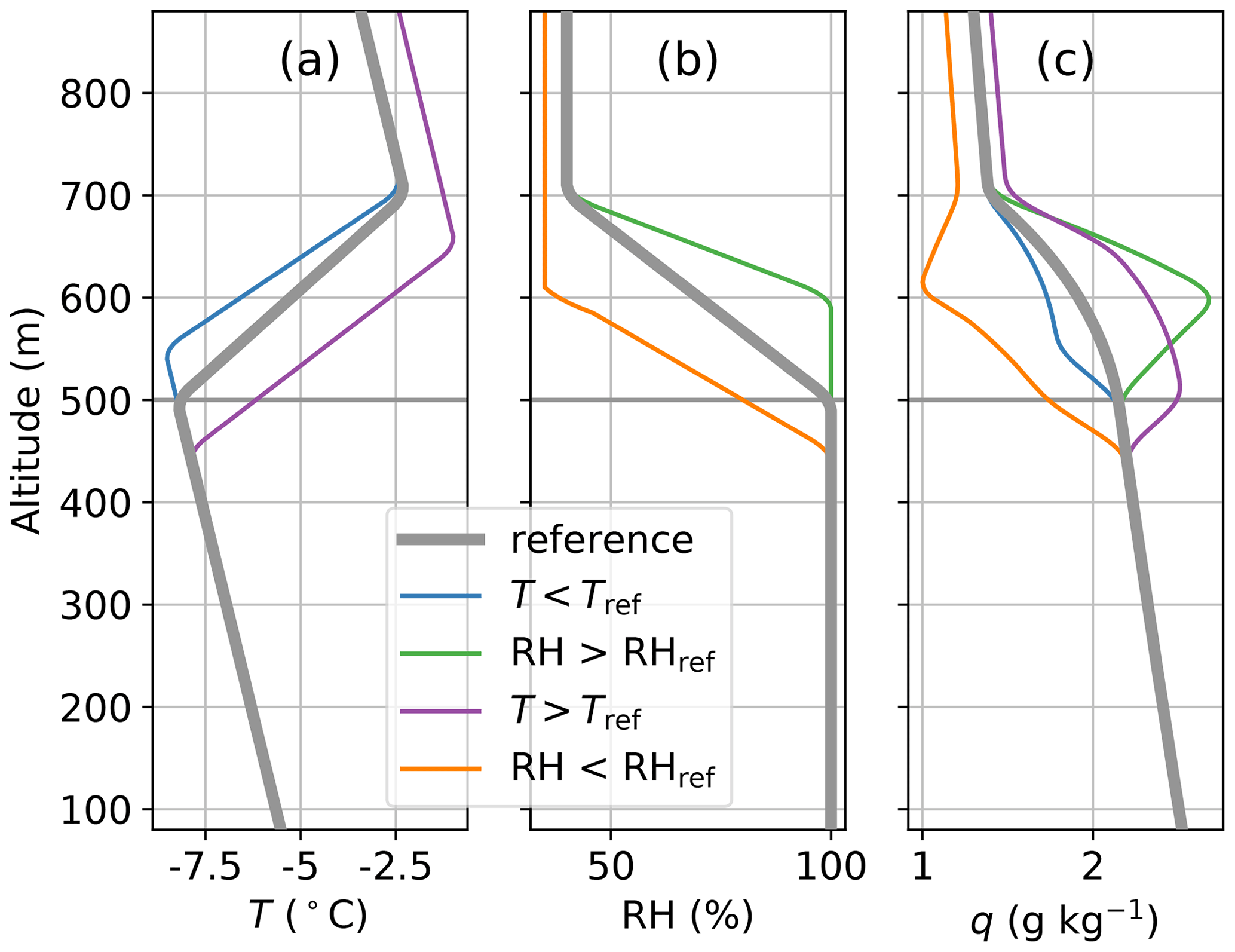
Figure 3 Sensitivity of the vertical q profile to a deviation of T and RH compared to a reference case (grey line). Only one parameter (T or RH) experiences a deviation in the inversion region, the other parameter is unchanged. Underestimated temperature (blue) or overestimated RH (green) might result from wet-bulbing. Overestimated temperature (purple) or underestimated RH (orange) might result from solar heating. A slow-response RH sensor overestimates RH on the ascent (green) and underestimates RH on the descent (orange).

As a second step, we simulate the influence of different time constants τ_RH and τ_T for the RH and temperature measurements. If both time constants have similar values, the resulting q does not change significantly in magnitude, but the vertical structure shifts upwards or downwards for an ascent or descent. With a slow-response RH sensor (τ_RH≫τ_T), the measured RH in the SHI region is overestimated on the ascent and underestimated on the descent with the effects on q as shown in Fig. 3c and with an artificial SHI on the ascent.

As a result of these sensitivity studies, the error in q is reduced when both the temperature and humidity sensors are affected by the same error source (e.g., solar heating on both sensors), and when both sensors have comparable time constants. Under these conditions, a detected SHI can be considered as most likely real and does not need to be interpreted as an artifact.

3.3 SHIs measured with BELUGA and radiosondes: natural feature or artifact?

A simple and convincing test of the possible influence of the error sources on the SHI observations is profiling in opposite direction, that is a descent from the free troposphere through the SHI into the cloud layer. This is commonly impossible in case of standard radiosoundings, but feasible for the BELUGA observations. Figure 4 shows vertical profiles of RH, T, and q as measured by radiosounding and BELUGA on 5 June 2017. Qualitatively, the measurements of both platforms show a similar vertical structure with a sharp temperature inversion capping the cloud layer. The cloud top (estimated from the observed downward terrestrial irradiance) is situated close to the temperature inversion base. However, the cloud top height derived from radiation observations should be treated with caution due to the vertical separation of the radiation and thermodynamic sensors by about 20 m, corresponding to a temporal shift between the observations of about 20 s during profiling. In the course of the measurement period of almost 2 h, the temperature inversion base and the cloud top remain at almost constant altitude. The radiosonde observation shows a layer of increased q between 400 and 550 m altitude just above the temperature inversion base. The increased specific humidity emerges from RH remaining high within the temperature inversion, before decreasing to the free troposphere level well above the inversion base.

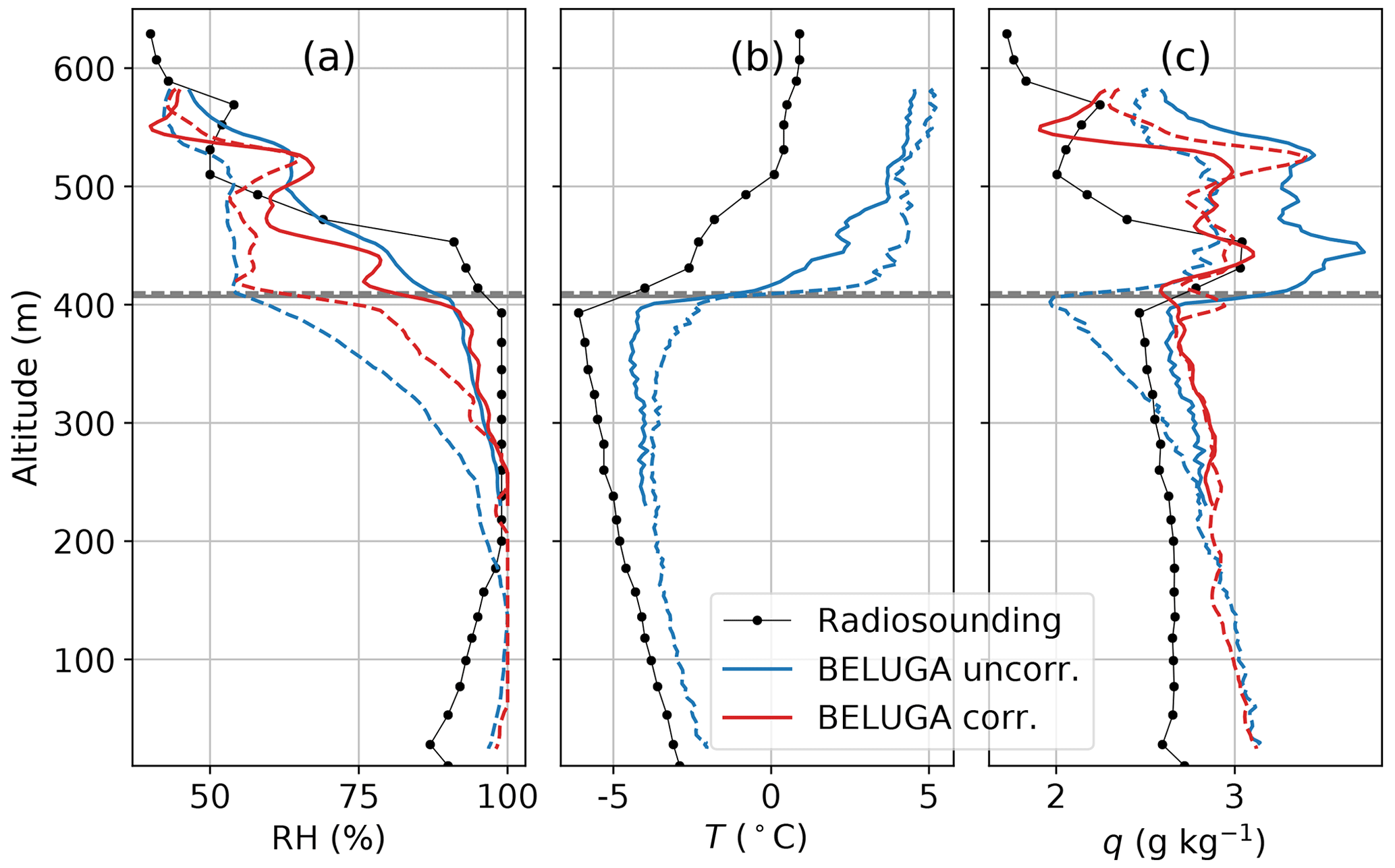
Figure 4 Vertical profiles of (a) relative humidity RH, (b) temperature T, and (c) specific humidity q measured by a radiosonde and BELUGA on 5 June 2017 (second profile). RH and q for BELUGA are shown before and after the corrections. The radiosonde was launched at 16:50 UTC; the balloon flew a continuous ascent and descent from 14:15 to 14:40 UTC. The cloud top (from BELUGA radiation data) is shown as horizontal lines. Solid and dashed lines represent the BELUGA ascent and descent, respectively.

Before comparing the q measurements from the radiosonde to BELUGA observations, we illustrate the effect of the applied RH correction and the consequences for the q profile. Figure 4a shows the uncorrected and time-response-corrected RH for an ascent and descent. The uncorrected RH ascent profile deviates strongly from the descent in the cloud top region. While descending through the cloud, the sensor requires a 150 m height difference for rising from 55 % to 95 % RH. The RH hysteresis around the cloud top is visible as a systematic deviation in all observed flight data (not shown). A comparison to Fig. 3 (orange lines) suggests that the major part of the error is due to a slow RH sensor. Furthermore, the sensor underestimates RH in the cloud on the descent, which might indicate solar heating. After applying the time lag correction, the RH profile shows a significantly reduced difference between ascent and descent. The remaining difference is qualitatively consistent with the temperature observations as shown in Fig. 4b. The temperature profiles show a warming of the cloud top and inversion region between 300 and 500 m during the descent leading to a reduced RH.

The “uncorrected” specific humidity in Fig. 4c is calculated from the uncorrected RH and the temperature measured with the fast-response thermocouple. The resulting q profiles show a SHI on the ascent and the descent of the BELUGA flight with a similar structure and location compared to the radiosonde data. The q profile as observed during the descent is shifted to lower q values in the region of the hysteresis of the uncorrected RH.

The corrected q results from the RH and the sensor-internal temperature T_s after correcting both signals for the time lag error according to Eq. (3). We argue that using T_s should be preferred instead of the thermocouple readings because RH and T_s have similar time constants, and RH is measured at T_s instead of the temperature of the atmospheric environment. The ambient temperature and T_s differ slightly due to the thermal inertia of the sensor housing.

After applying the corrections, the maximum value of the SHI, as observed during the BELUGA ascent, is reduced by about 0.6 g kg⁻¹ compared to the uncorrected q maximum. After correction, all BELUGA profiles and the radiosonde data exhibit the SHI with similar structure and amplitude. This consistency suggests that the observed SHI is a natural feature instead of an instrumental artifact. We can exclude wet-bulbing as the main reason for the observed SHIs because the SHI is also present during the descent. The influence of solar heating and time-lag errors is minimized. Our conclusion also strengthens the confidence in SHIs as frequently observed by radiosondes.

4 Vertical profiles of mean ABL parameters

4.1 Comparison of normalized temperature and humidity profiles

Throughout the observation period, we observe a persistent layer of increased specific humidity above the cloud layer. One of the governing questions of this analysis is to understand how observed SHIs relate to the general ABL structure and, in particular, to the temperature inversion. Figure 5a and b shows vertical profiles of potential temperature θ and specific humidity q recorded in the period of 5–7 June 2017. Both parameters are normalized to their near-surface values and plotted in relation to the base height of the temperature inversion z_i. The cloud boundaries are shown in Fig. 5c for reference.

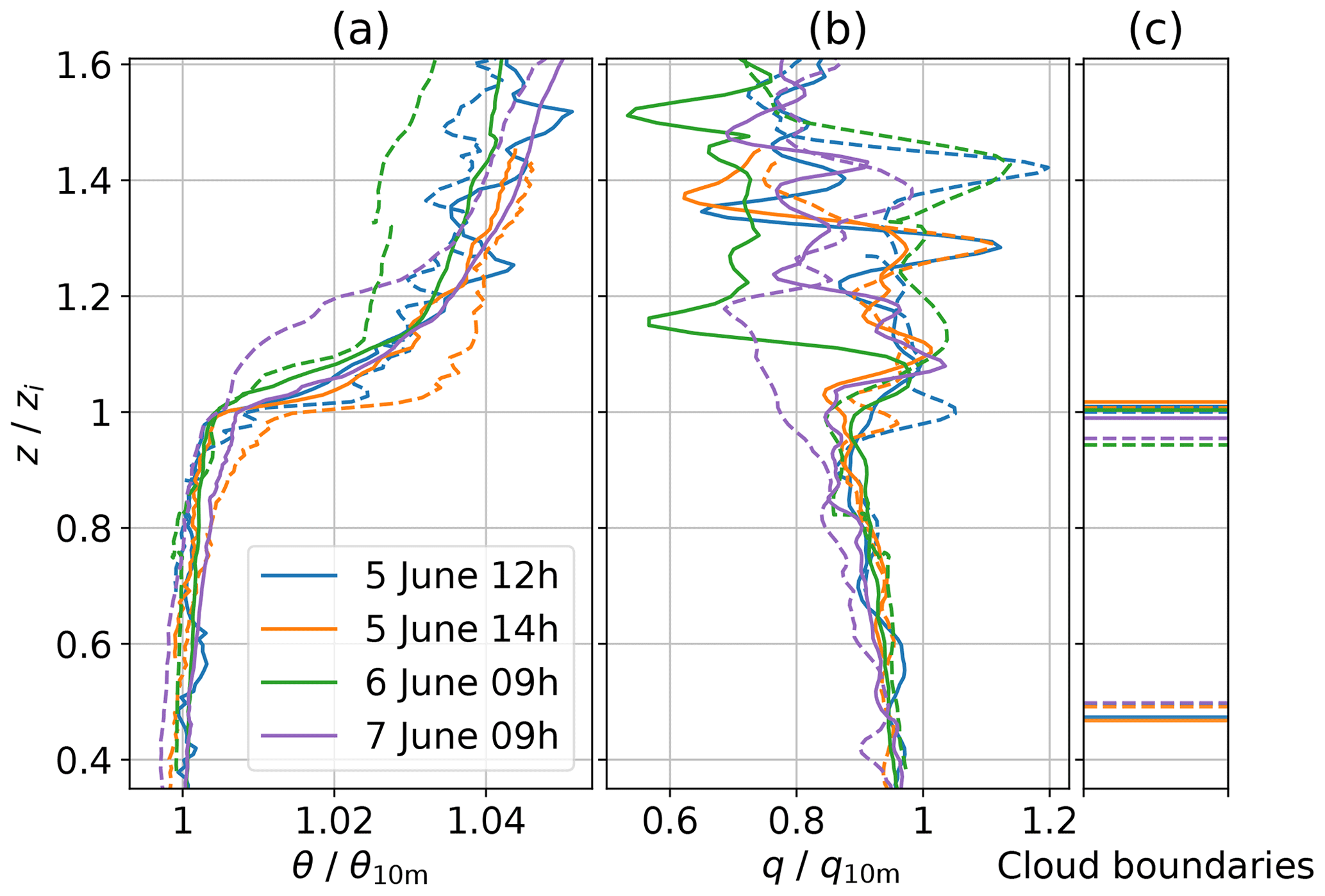
Figure 5 Balloon-borne vertical profiles of (a) potential temperature θ, (b) specific humidity q, and (c) cloud boundaries for four ascents (solid lines) and descents (dashed lines) on 5, 6, and 7 June 2017. The altitude z is normalized to the temperature inversion base height z_i. Potential temperature θ and the specific humidity q are normalized to their near-surface values. The cloud top is derived from the irradiance profile; the cloud base is derived from Cloudnet data. The profiles are named after the start time (cf. Fig. 2).

All measurements show a similar vertical structure of θ within the ABL. Below the temperature inversion base z_i, the stratification is near-neutral to weakly stable. Above the inversion, the thermodynamic stability is higher and exhibits more variability compared to below the inversion. No systematic difference between ascents and descents is visible. The ABL is thermodynamically coupled to the surface, which makes normalizing to surface values meaningful.

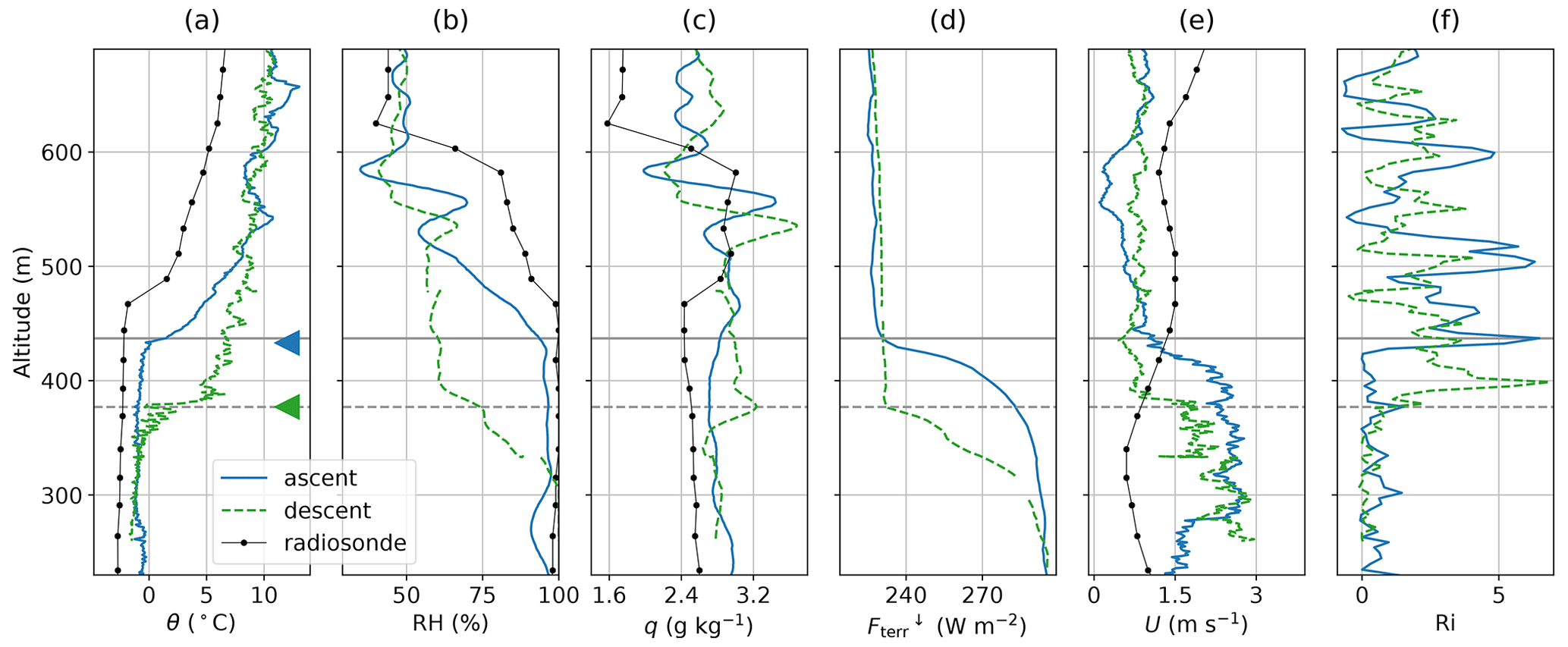
Figure 6 Boundary layer observations around the cloud top on 5 June 2017, first profile: vertical profiles of (a) potential temperature θ, (b) RH, (c) specific humidity q, (d) downward terrestrial irradiance $F_{\text{terr}}^{\downarrow }$, (e) horizontal wind velocity U, and (f) Richardson number Ri for BELUGA ascent and descent and the radiosonde launched at 11:00 UTC. The triangles indicate where z_i is defined. The cloud top is shown as horizontal lines (solid for ascents and dashed for descents).

Within the mixed layer below z_i, specific humidity decreases slightly with height but increases when reaching z_i. Above z_i, the normalized specific humidity exhibits more variability compared to the normalized temperature. The descent of 7 June 09 h shows a temperature inversion with some internal structure in the form of two smaller “steps” in θ. We define z_i at the lower step, with the SHI base being located clearly above at the upper step at $z\approx \mathrm{1.2}\cdot z_{\mathrm{i}}$. For this case, a deficit in q is observed below the SHI, which is plausible because between ascent and descent cloud top had decreased to about 0.95⋅z_i.

For most profiles, the cloud top coincides with z_i, and the increased humidity is observed above the cloud layer. Only for two profiles (both descents on 5 June), the lower bound of the SHI is already located below the cloud top. We do not find clouds penetrating into the temperature inversion, although such situations have been frequently observed in previous studies (e.g.,  Pleavin, 2013; Sedlar et al., 2012; Sedlar and Shupe, 2014; Shupe et al., 2013; Brooks et al., 2017). However, two of the descent profiles (6 June 09 h and 7 June 09 h) show situations where the cloud top had decreased between ascent and descent, and the SHI is vertically separated from the cloud top.

4.2 Cloud top variability versus SHI height

The cloud top variability, here defined as the cloud top height difference between ascent and subsequent descent for each profile, is related to z_i and the lower boundary of the SHI. For all 3 d, a descending cloud top is observed between the ascent and subsequent descent with a cloud top height difference of 50 to 100 m. This cloud top variability is indicated by in situ irradiance and thermodynamic measurements and also confirmed by radar reflectivity (cf. Fig. 2). In order to illustrate the relation of cloud top height, SHI, and other ABL parameters, Figs. 6–8 show profiles of mean θ, RH, q, downward terrestrial irradiance $F_{\text{terr}}^{\downarrow }$, horizontal wind velocity U, and Richardson number Ri as measured during ascents and descents on 5, 6, and 7 June, respectively. We analyze only continuous profile data without longer breaks at certain heights for the first profile of each day. The cloud top height is defined by the discontinuity of the $F_{\text{terr}}^{\downarrow }$ profile and marked with horizontal lines, whereas z_i is indicated with triangles. The Richardson number is the ratio between thermodynamic stability and wind shear and, therefore, a measure for the ability of turbulence generation (Ri ≲ 1) or dissipation (Ri ≳ 1).

On 5 June (Fig. 6), z_i lowers from 430 to 380 m in the course of the BELUGA flight. The temperature difference across the inversion of Δθ≈9 K, which is also the strongest observed during our flights, stays constant during ascent and descent. The RH decreases within the temperature inversion, accompanied by an increase in q above z_i of about 0.25 g kg⁻¹ (ascent) and 0.5 g kg⁻¹ (descent). The radiosonde, launched around 2 h prior to the BELUGA flight, shows a higher z_i but qualitatively a similar vertical structure of θ, RH, and q. The cloud top agrees well with z_i for the ascent and descent. The horizontal wind velocity U is around 2 m s⁻¹ inside the cloud layer and decreases to 1 m s⁻¹ in the free troposphere, resulting in horizontal wind shear. During the ascent, the wind shear zone is clearly located below z_i with a sudden increase in Ri to values greater than 1 above z_i and cloud top. During the descent, the strongest wind shear is observed around z_i, and the resulting increase in Ri is slightly above z_i. This vertical shift suggests a slightly stronger turbulent coupling between cloud top and the SHI above, as compared to the ascent.

Figure 7 Same as Fig. 6, but for 6 June 2017 (first profile).

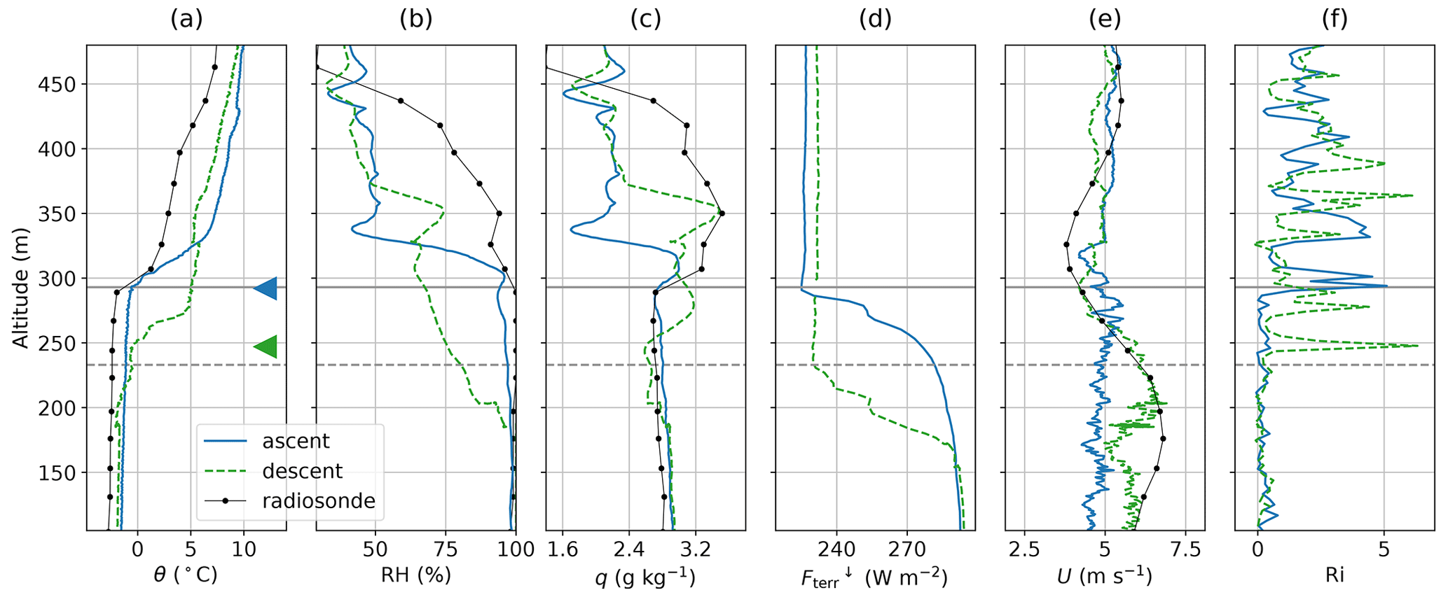
The general ABL structure observed on 6 June (Fig. 7) in terms of the profiles of θ, RH, and q is quite similar to the 5 June observations, showing a decreasing cloud top height during the balloon operation. Here, z_i decreases from 290 m during the ascent to about 230 m during the descent. The radiosonde, launched 1.5 h after the BELUGA flight, shows a similar z_i to the balloon ascent, indicating that z_i and cloud top recover between BELUGA descent and radiosounding. This is in agreement with the radar observations in Fig. 2. The lower bound of the SHI with $\mathrm{\Delta }q\approx \mathrm{0.3}\mathrm{g}{\mathrm{kg}}^{-\mathrm{1}}$ on the ascent and 0.7 g kg⁻¹ on the descent is coupled to z_i in both cases. On the ascent, z_i coincides with the cloud top. During the descent, the cloud top is almost 20 m below z_i, which could possibly result from cloud top heterogeneity. However, the temperature gradient is smoother compared to the ascent, which leads to a less clear determination of z_i. The humidity structure above the cloud layer observed by the radiosonde exhibits a distinct SHI with a lower bound coupled to the temperature inversion. Peak values of q are comparable with BELUGA observations made during the descent. The horizontal wind velocity is about 5 m s⁻¹ and almost height-constant for the entire ascent but increases by about 2 m s⁻¹ inside the cloud layer during the descent. The radiosonde provides a similar picture to the balloon descent. For the ascent, the sharp increase in Ri is connected to z_i, whereas for the descent this increase in Ri is – similar to the previous day – about 20 m above cloud top, allowing for some turbulent exchange between the cloud and the SHI above.

Figure 8 Same as Fig. 6, but for 7 June 2017.

On 7 June, a clear SHI develops with a lower boundary at around 580 m, which is similar in the two BELUGA and the radiosonde profiles (Fig. 8). For the BELUGA ascent and the radiosonde profile, this boundary agrees well with z_i and cloud top (for the radiosonde data cloud top can be roughly estimated from the RH profile). The radiosonde profile and BELUGA ascent are shifted in time by about 70 min and the remarkable match in z_i should not be over-interpreted. For the BELUGA descent, the thermal stratification changes again (similar to the previous days). The temperature inversion weakens and z_i is shifted downward by about 110 to 480 m, together with the cloud top. Thus, the cloud top and the SHI base are separated by 110 m on the descent. The terrestrial irradiance inside the cloud layer fluctuates strongly, especially on the descent, which suggests a patchy cloud with cloud holes. The horizontal wind velocity agrees qualitatively for all three profiles. Inside the ABL, a higher wind velocity of around 6 m s⁻¹ is observed with the BELUGA observations, showing a local maximum of 8 m s⁻¹ slightly below z_i. Above this maximum, U gradually decreases to 2 m s⁻¹ in the free troposphere. According to the Richardson number, wind shear limits turbulence above the cloud top for both ascent and descent.

To resume, we observed mean profiles of several cases where cloud tops coincide with z_i and the SHI base. Although some cloud tops show more or less strong horizontal wind shear, the stabilizing effect of the temperature inversion leads to a sudden increase in Ri just above the cloud layer, which suggests a rather low turbulent exchange with the humidity layers above. However, for one case a special situation provides a new aspect of this phenomenon: z_i and cloud top height had decreased while the humidity layer remained at its vertical position, leading to a humidity gap between cloud top and SHI.

5 Turbulence at cloud top and around the SHI

Concerning the question of how the humidity and cloud layer interact and to what extent these layers exchange energy by turbulent transport, we first describe the interface between the SHI and cloud top by means of observations at constant altitude (Sect. 5.1). We then analyze the vertical profiles of basic turbulence parameters (Sect. 5.2) and turbulent energy fluxes (Sect. 5.3).

5.1 Observations at constant altitude in the inversion layer

To get an insight into the transition from cloud top to the humidity layer above, measurements were taken at a constant height in the temperature inversion region. Figure 9 shows a 500 s time series measured on 6 June at a constant altitude around z_i≈300 m (second last constant altitude segment in Fig. 2 for 6 June). The local dissipation rate ε is evaluated in 2 s segments to illustrate the evolving turbulence intensity.

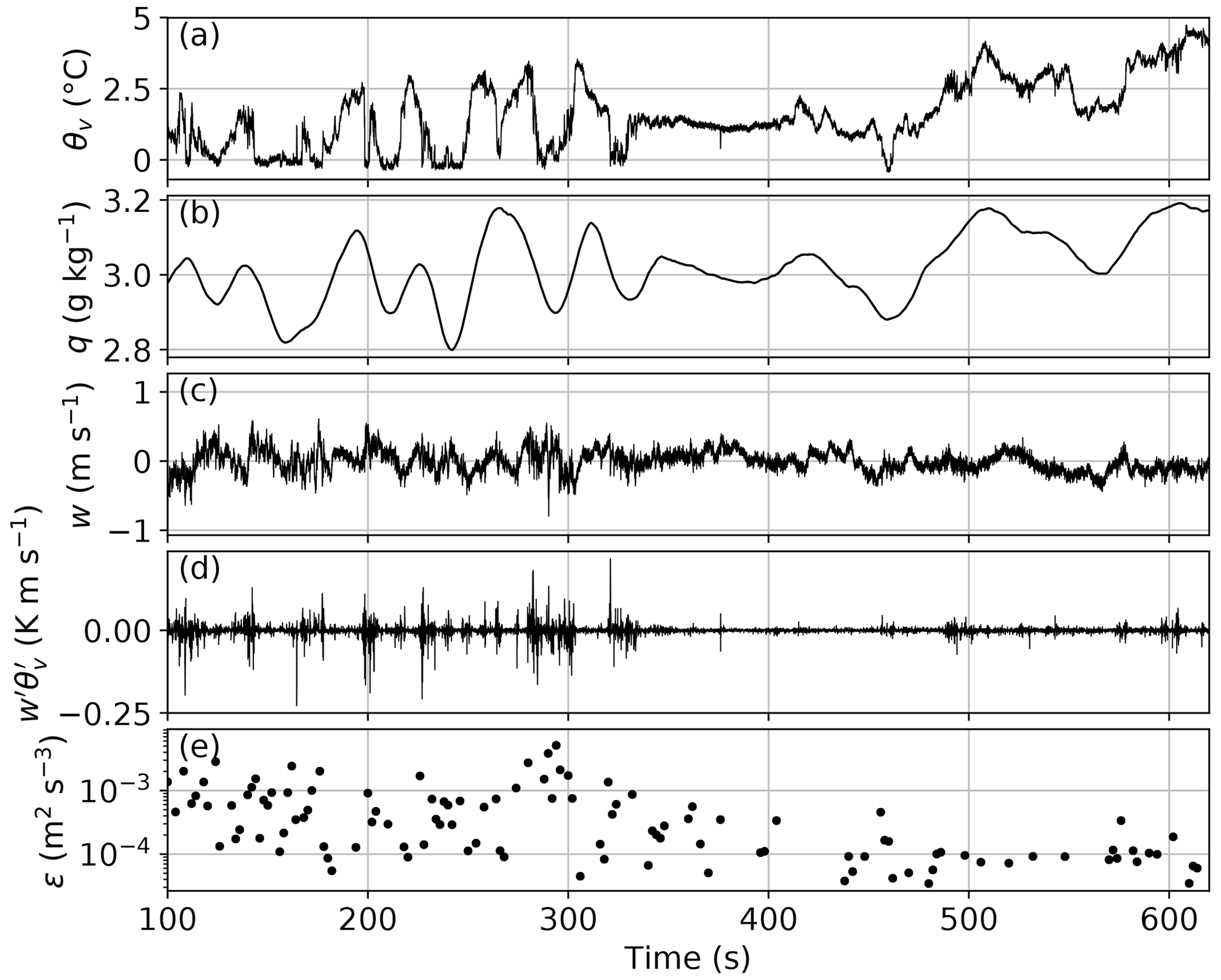
Figure 9 Constant-altitude time series of (a) virtual potential temperature θ_v, (b) specific humidity q, (c) vertical wind w, (d) co-variance ${{\mathit{\theta }}_{\mathrm{v}}}^{\prime }{w}^{\prime }$, and (e) dissipation rate ε for 6 June measured at 300 m altitude around z_i.

Within the first third of the record, the virtual potential temperature θ_v (as approximately measured by the ultrasonic anemometer) shows strong variations on a typical timescale of 30–50 s with amplitudes up to 3 K. Based on the temperature gradient (Fig. 7), the changes in θ_v would correspond to a height variation of ∼10 m. More likely, parts of the height-constant measurements (Δz≈1 m) are taken in potentially colder, drier, and more turbulent air masses at the inversion base, interrupted by measurements in potentially warmer, more humid, and less turbulent air masses at higher altitudes well within the T inversion. This variability is also visible in the wind direction (not shown here). Depending on the relative location of z_i to the measurement height, the co-variance $w^{\prime }{\mathit{\theta }}_{\mathrm{v}}^{\prime }$ is highly intermittent and no mean flux is derived from these observations.

The center part of the record is characterized by a comparably low variability leading to the conclusion that this part of the observations is performed entirely inside the descending temperature inversion. Finally, observations are performed well above z_i inside the stably stratified T inversion layer, characterized by values of ε 1 order of magnitude lower compared to at the inversion base. Here, variations in θ_v and q are again correlated and caused by changes in relative height.

The observations do not allow for drawing quantitative conclusions, such as time and area-averaged turbulent heat fluxes, from this record. However, these measurements vividly illustrate the difficulties in estimating turbulent fluxes based on covariance methods in the vicinity of the temperature inversion, although the measurement height is kept at a remarkably constant height level. Therefore, the methods for estimating turbulent fluxes based on mean vertical gradients and slant profiles are more suitable for this study and are used below.

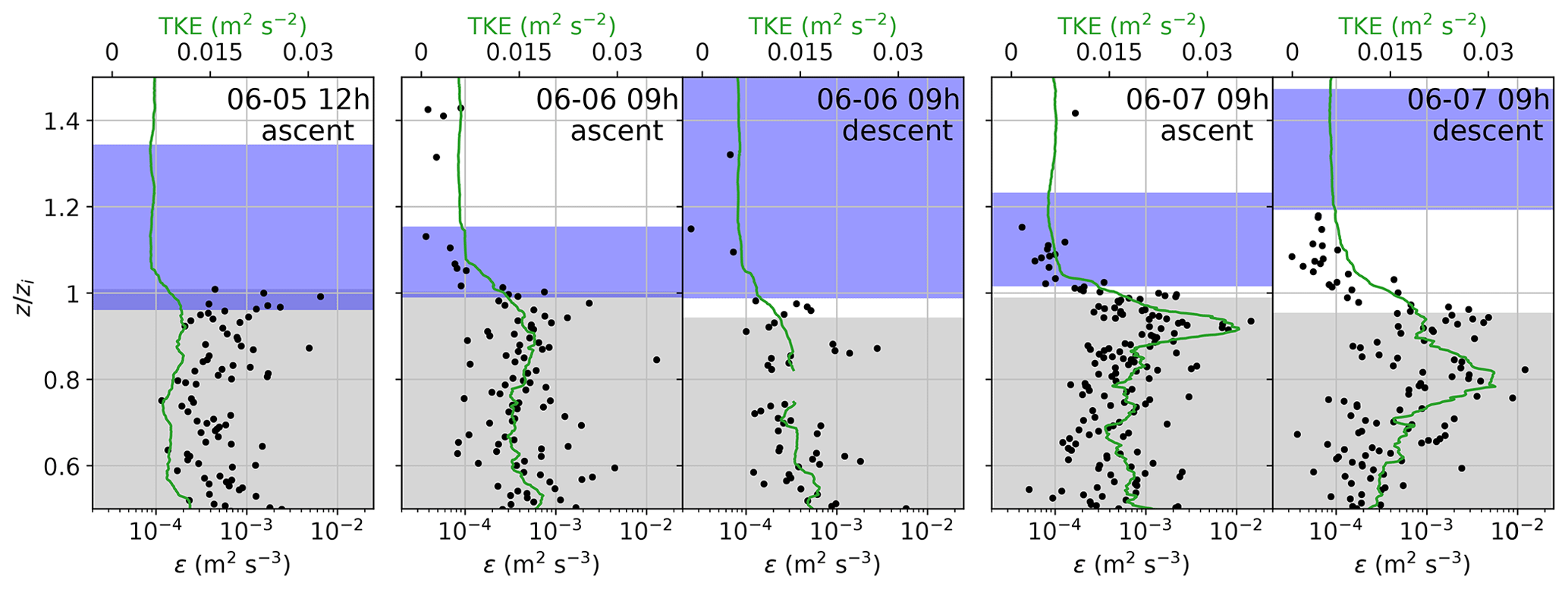
Figure 10 Vertical profiles of local dissipation rate ε and TKE for the first ascent and descent of 5, 6, and 7 June 2017. The height is normalized by the temperature inversion base z_i. The region of increased specific humidity is marked as blue shading, the cloud layer as grey shading.

5.2 Vertical profiles of turbulent energy and dissipation

The vertical distribution of turbulence parameters, such as local dissipation rate ε and the turbulent kinetic energy TKE, provide an insight into the coupling between the cloud layer and the SHI. The local ε values are derived from second-order structure functions by applying inertial subrange scaling as described by Egerer et al. (2019a). Different from that study, here ε is calculated from non-overlapping, 2 s sub-records yielding a vertical resolution of about 2 m. Regions without inertial sub-range scaling are excluded. Turbulent kinetic energy ($=\mathrm{0.5}\cdot u_i^{\mathrm{2}}$) is calculated in a moving 50 s window. The observed TKE noise level is about 0.005 m² s⁻² and is usually reached at $z/z_{\mathrm{i}}$ ≳ 1.1.

Figure 10 shows ε and TKE for each first profile of 5, 6, and 7 June as a function of normalized height (the descent of 5 June is excluded due to data issues). The cloud and humidity layers are shaded for reference. For the presented cases, turbulence is most pronounced in the upper cloud layer and around cloud top with typical values of $\mathit{\epsilon }\sim {\mathrm{10}}^{-\mathrm{3}}$ m² s⁻³ and TKE ∼ 0.02 m² s⁻². For 5 and 6 June, the turbulence intensity is rather constant in the cloud. For 7 June, with increased wind velocity, a maximum of ε is evident just below cloud top.

Figure 10 also illustrates how the SHI and cloud layer are either separated or overlap, and how they are connected by turbulent motion. At a certain height level, ε decreases to the low-turbulence free-troposphere level. The transition is gradual, indicating turbulent mixing in this region. On 5 June and the ascents of 6 and 7 June, the SHI and the cloud are directly coupled by turbulent mixing. For the descents of 6 and 7 June, most of the mixing takes place at the interface of the cloud top with the humidity gap between cloud and SHI. In this case, inside the SHI the turbulence intensity is reduced almost to the free-troposphere level and the SHI seems to be decoupled from the cloud layer via the humidity gap in between.

We can only speculate about the reason for the development of this humidity gap, which is most pronounced for the descent of 7 June. One explanation could be long-range advection of increased moisture in the free troposphere combined with a temporary collapse of the well-mixed cloud layer leading to a vertical separation of cloud top and SHI. However, this interesting feature leads to new research questions that require further observations and a more detailed LES analysis.

5.3 Vertical profiles of turbulent moisture and heat fluxes

The turbulent exchange of moisture can be quantified by the latent heat flux

$$\begin{array}{}\text{(4)}& {\displaystyle }{\displaystyle }L=\stackrel{\mathrm{‾}}{\mathit{\rho }}\cdot L_{\mathrm{v}}\cdot \stackrel{\mathrm{‾}}{w^{\prime }{q}^{\prime }},\end{array}$$

whereas the virtual sensible heat flux is given by

$$\begin{array}{}\text{(5)}& {\displaystyle }{\displaystyle }H=\stackrel{\mathrm{‾}}{\mathit{\rho }}\cdot c_p\cdot \stackrel{\mathrm{‾}}{w^{\prime }{\mathit{\theta }}_{\mathrm{v}}^{\prime }},\end{array}$$

with an overline describing an average of the sub-record. Here, $\stackrel{\mathrm{‾}}{\mathit{\rho }}$ is the mean air density, $L_{\mathrm{v}}=\mathrm{2.5}\times {\mathrm{10}}^{\mathrm{6}}\mathrm{J}{\mathrm{kg}}^{-\mathrm{1}}$ is the latent heat of evaporation, and c_p=1005 $\mathrm{J}{\mathrm{kg}}^{-\mathrm{1}}{\mathrm{K}}^{-\mathrm{1}}$ is the specific heat capacity of air. This direct calculation of H and L requires sufficient long, stationary, and homogeneous records in a certain height to provide time-averaged estimates of the covariances with statistical significance (Stull, 1988; Lenschow et al., 1994). Our observations focus mainly on vertical profiling, and only a limited number of height-constant records around the cloud top and inversion region are available. As shown in Sect. 5.1, the conditions around the temperature inversion are highly instationary and, thus, we use the vertical profiles to study the fluxes in this region. We apply two approaches for estimating fluxes from vertical profiles: (i) describing the flux profile by applying the so-called “slant profile method” and (ii) relating the turbulent flux to mean gradients (flux gradient method).

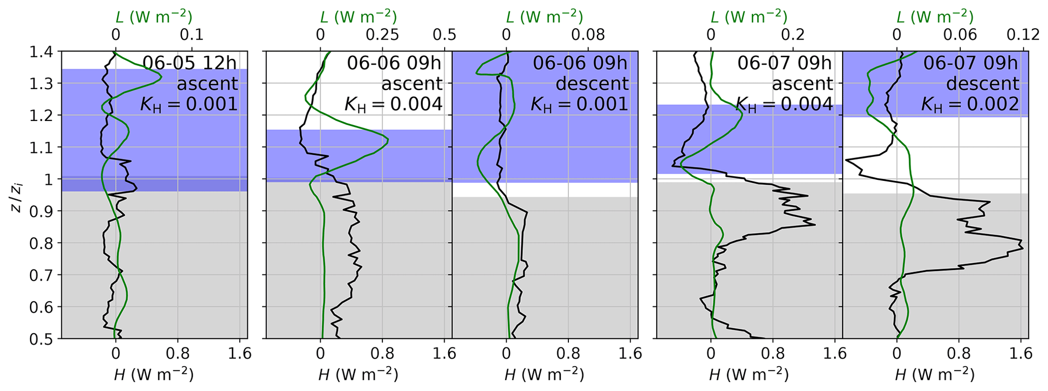
Figure 11 Same as Fig. 10, but for the virtual sensible heat flux H (eddy covariance method) and the latent heat flux L (flux gradient method).

The slant profile method is based on the assumption that for a certain height range the profile data are considered as a homogeneous record and Eq. (5) can be applied. For this method, instantaneous values of H are estimated for a defined height range, defining also the length scales contributing to the flux. For our observations, this method provides only results for H due to the lack of fast-response humidity measurements. Alternatively, L can be estimated with the flux gradient method. This method is based on the relation between the covariances and the mean gradients of θ_v and q:

$$\begin{array}{}\text{(6)}& {\displaystyle }{\displaystyle }\stackrel{\mathrm{‾}}{w^{\prime }{\mathit{\theta }}_{\mathrm{v}}^{\prime }}=-K_H\cdot {\displaystyle \frac{\partial {\stackrel{\mathrm{‾}}{\mathit{\theta }}}_{\mathrm{v}}}{\partial z}},\end{array}$$

and

$$\begin{array}{}\text{(7)}& {\displaystyle }{\displaystyle }\stackrel{\mathrm{‾}}{w^{\prime }{q}^{\prime }}=-K_Q\cdot {\displaystyle \frac{\partial \stackrel{\mathrm{‾}}{q}}{\partial z}},\end{array}$$

with K_H and K_Q being the turbulent exchange coefficients for sensible and latent heat, respectively. The coefficients are defined as positive, which means that the flux is directed against the mean gradient. Values of K can be derived from parameterizations based on turbulence observations such as proposed by Hanna (1968) or by directly applying Eq. (6) with the measured H, yielding K_H. With K_Q≈K_H (Dyer, 1967) for a wide range of stratification and the mean humidity gradient $\partial \stackrel{\mathrm{‾}}{q}/\partial z$, we estimate L by combining Eqs. (7) and (4).

Before estimating H from the slant profiles by applying Eq. (5), the turbulent fluctuations must be determined. This is done by applying a high-pass filter of Bessel type with a filter window of 10 s, corresponding to a horizontal length scale of about 10 to 70 m (depending on the horizontal wind velocity) and a vertical length scale of about 10 m. After filtering, the fluxes are averaged over a moving 50 s window by applying Eq. (5). The filter and averaging windows are similar to the values proposed by Tjernström (1993) and Lenschow et al. (1988), who estimated turbulent fluxes from aircraft-based slant profiles.

Figure 11 shows five selected cases (cf. Fig. 10) with profiles of H based on the slant profile method and L based on the flux gradient method. The upper part of the cloud layer is mainly characterized by an upward-oriented heat flux (H>0), most pronounced for the last two profiles with a local maximum between $\mathrm{0.8}<z/z_{\mathrm{i}}<\mathrm{1}$. Only for the first ascent of 5 June is the H flux almost height-constant with much lower values compared to the other days. For this day, θ_v exhibits larger variability around and slightly above z_i, which differs from the typical structure of a turbulent flow. This variability mainly causes the positive values of H around z_i, which, therefore, should not be misinterpreted. This is a similar effect to that discussed in Sect. 5.1. A negative peak of H around or slightly above z_i is visible for the descent of 6 June and both profiles of 7 June. On 7 June, a secondary, weaker negative peak in H is located at the lower part of the SHI.

Although it is known that in general K=K(z), we estimate a constant K_H for each ascent and descent in the lower region of the SHI, which is the focus area of our study. In that region, we observe negative H fluxes and positive θ_v gradients. Applying Eq. (6) leads to mean values of K_H between 0.001 and 0.004 m² s⁻¹ for the five profiles. The K_H(=K_Q) values for each profile are used for calculating the L profile based on the flux gradient method.

A negative peak in L is observed for all days in the lower SHI region. The downward energy flux at cloud top is common for the entrainment region, where potentially warmer and usually drier air from the free troposphere is mixed downward into the (cloudy) ABL. However, for our observations, this downward flux in the lower SHI region means a downward transport of potentially warmer but more humid air into the region below. The situation is different for the descent profile of 7 June, with the vertical humidity gap between cloud top and SHI. Here, the negative peak in L at the lower SHI is accompanied by a positive L at cloud top. This profile does not suggest a significant transport of humidity into the cloud top. Instead, for the special case where the cloud and the SHI are separated, the gap in between receives moisture from both the SHI above and from the cloud layer below.

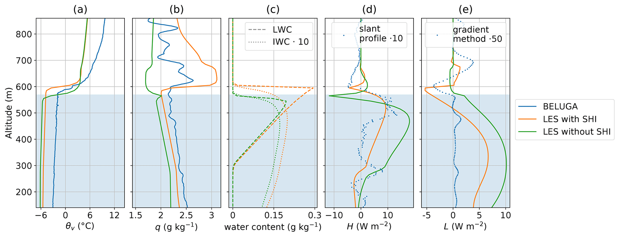
Figure 12 LES results (with and without an initial SHI) and BELUGA observations for 7 June 2017: vertical profiles of (a) virtual potential temperature θ_v, (b) specific humidity q, (c) liquid (LWC) and ice water content (IWC), (d) virtual sensible heat flux H, and (e) latent heat flux L. The light blue area is the cloud extent for the observations (cloud top is derived from BELUGA irradiance measurements, cloud base from lidar data).

6 Possible influence of the humidity layer on ABL and cloud structure: an LES study

The observational data discussed so far provide insight into the turbulent structure of cloudy ABLs that are capped by humidity layers. What remains unclear is how the presence of such humidity layers might have impacted the general ABL and clouds as observed on this day. For this purpose numerical experiments at cloud- and turbulence-resolving resolutions can be used to good effect, providing virtual datasets for detailed process studies and allowing sensitivity tests for hypothesis testing (Solomon et al., 2014). In this section idealized Lagrangian large-eddy simulations (LESs) are discussed that were generated to match the observed vertical structure of the ABL as closely as possible. For a detailed technical description of the experimental design of these realizations, we refer to Appendix B. Two simulations are discussed, one based on an initial profile without a SHI, the other with a SHI superimposed. The LES simulations are Lagrangian, following an air mass from a location 12 h upstream of the RV Polarstern. This allows for proper model spinup and also gives the SHI ample time to impact the turbulence and clouds below. The simulations are sampled when the air mass arrives at RV Polarstern on 7 June 2017 at 10:48 UTC. The LES output considered includes the mean thermodynamic and cloudy state, as well as the turbulent fluxes of heat H and moisture L, calculated as the covariance between vertical velocity and perturbations in static energy and humidity, respectively.

Figure 12 shows vertical profiles of the LES output (with and without an initial SHI) and the BELUGA ascent, where cloud top, z_i, and SHI base coincide. The LES profiles represent averages over the horizontal domain over a 900 s period. The temperature differences across the inversion as well as the lapse rates above are reasonably well reproduced by the LES (Fig. 12a). The experiment including an initial SHI features a temperature inversion base z_i, and similarly a mixed-layer depth, that agrees well with the observations. Without the initial humidity layer, z_i is approximately 40 m lower. The vertical profile of specific humidity shows a similar vertical structure and a distinct increase in q above the cloud layer in both the model and the observations (Fig. 12b). The strength of the SHI of Δq=1.1 g kg⁻¹ in the LES is close to the radiosonde SHI strength of Δq=0.9 g kg⁻¹, but larger than the SHI observed with BELUGA of Δq=0.6 g kg⁻¹. In the LES without initial SHI, specific humidity decreases by Δq≈0.2 g kg⁻¹ within the temperature inversion height range. Within the mixed layer, both experiments slightly underestimate θ_v and q compared to the BELUGA soundings. This is probably explained by the calibration of these experiments to the radiosonde soundings, which show a similar offset compared to BELUGA (cf. Fig. 8).

Compared to the balloon measurements, a thinner liquid cloud layer forms in the LES, as indicated in the LWC profiles in Fig. 12c. While the observed mixed-phase cloud is around 500 m thick, the simulations result in a liquid cloud of about 300 m vertical extent. Note that significant ice water is present below the liquid cloud base in the model, for which lidar readings are sensitive (Bühl et al., 2013). For this reason, the model bias in cloud base height could be artificial. Without a humidity layer, the liquid cloud is thinner, extending only 260 m. The cloud top is simulated at around 600 m altitude for the scenario with SHI and at 560 m altitude for the scenario without SHI, respectively. In the SHI case, the higher cloud top reflects the larger mixed-layer depth compared to the case without SHI.

The LES provides a positive (i.e., upward-directed) virtual sensible heat flux inside the cloud layer (Fig. 12d). The negative virtual heat flux at cloud top is seen with and without initial SHI. The LES, with or without an initial SHI, shows a positive moisture flux L between surface and cloud top (Fig. 12e). In the presence of an initial SHI, the cloud top region exhibits a negative moisture flux. This negative moisture flux coincides with the negative virtual sensible heat flux and indicates that downward humidity transport takes place between the humidity layer and the underlying mixed layer. Lacking the initial SHI, the total moisture flux is close to zero near the inversion. This means that in this case dry air, rather than humidity, is entrained into the mixed layer from above. The direction of fluxes is in agreement with the flux estimates in Sect. 5.3 for 7 June, where a SHI is present above cloud top on the ascent.

More research is necessary to further investigate how the additional entrained moisture of the humidity layer is processed in the cloud (e.g., through phase transition) and how exactly the humidity layer contributes to the cloud evolution (e.g., the role of clouds penetrating into the inversion or thermodynamically decoupled clouds).

7 Summary and conclusion

A persistent layer of increased specific humidity above a stratocumulus deck has been observed by tethered-balloon-borne instrumentation in the Fram Strait northwest of Svalbard (82^∘ N, 10^∘ E) in the period from 5 to 7 June 2017. Vertical profiles of thermodynamic parameters, wind velocity, and terrestrial irradiance were sampled in situ. An in-depth discussion of the problems associated with humidity measurements in cloudy and cold environments led to the conclusion that the observed SHIs are a natural feature and not a result of measurement artifacts. The high resolution of the measurements allows for estimating local turbulence parameters such as local energy dissipation rates. Based on slant profiles, the turbulent virtual sensible heat flux was estimated by applying the eddy covariance method. The vertical profile of the latent heat flux was calculated by applying the flux gradient method. The observations allow for the first time detailed analyses of the relative position of the SHI, cloud top, and the temperature inversion height z_i and give a first qualitative indication of how these different layers are coupled by turbulent transport.

We observed two different scenarios: (i) the base of the SHI qualitatively coincides with z_i and the cloud top height and (ii) cloud top height and z_i had decreased with the SHI base remaining at a constant height, leading to a “humidity gap” between cloud top and SHI base. Turbulence, as described by local ε, decreases gradually above z_i suggesting that turbulent energy exchange is possible in that region. Vertical profiles of latent heat fluxes qualitatively show a downward moisture transport at the base of the SHIs for all profiles. When the SHI coincides with the cloud top as in the first scenario (i), this suggests the cloud is being supplied with moisture from the overlying SHI. For the second scenario (ii), the sign of the latent heat fluxes suggests upward humidity transport from the cloud together with downward humidity transport from the SHI base, both feeding the vertical gap between the SHI base and the cloud top with moisture.

For one case study of the first type of scenario, LESs were performed. The simulations support the observational findings by showing a negative moisture flux at the SHI base towards the cloud region below. Further, the LESs show that the moisture supply does directly influence the dynamics of the cloudy ABL by increasing z_i and the cloud layer thickness.

For more general conclusions beyond case studies, further observations over a larger measurement period are necessary. An improvement for future measurements would be a fast-response humidity sensor that operates reliably under cold and cloudy conditions. Those observations would allow for quantifying the vertical moisture transport by applying the eddy covariance method instead of relying on estimating the exchange coefficient and mean humidity gradients.

Furthermore, we suggest a thorough LES study driven by our observations. These studies are capable of investigating the consequences of the two observed scenarios on ABL dynamics and cloud lifetime and will help to answer the question of how important the SHIs are for the Arctic cloudy ABL.

Appendix A: Estimating the time constants of the BELUGA humidity sensor

Figure A1 Time response of the humidity sensor to a step function experiment: (a) sensor-internal temperature T_s and (b) RH at 8.6 m s⁻¹ with fitted time constants τ. Panel (c) shows the time constants depending on the flow speed. A root fit function is added to the values.

We determine the time constants for the BELUGA humidity sensor in laboratory experiments by analyzing the sensor response to a step-like change of the surrounding thermodynamical parameters. The sensor is brought from a calm and saturated environment into a sub-saturated airstream with constant T and RH. The flow speed of the sub-saturated air is varied between 2 and 9 m s⁻¹. In addition to RH, the sensor provides a measure for the internal sensor temperature T_s, which is determined by a PT-1000.

Figure A1a and b show an example for the time response of the humidity sensor on BELUGA. The time constants τ_RH and ${\mathit{\tau }}_{T_{\mathrm{s}}}$ are obtained from an exponential fit to the response function at a constant flow speed of 8.6 m s⁻¹. Figure A1c summarizes the resulting time constants for different flow speeds. The time constant of a temperature and RH sensor is influenced by the heat and moisture transfer, which scale with the flow speed $\propto \mathrm{1}/\sqrt{U}$ (e.g., Bruun, 1995, for heat transfer). Based on this relationship, a least-square fit to the observations yields the τ values depending on the flow speed. For flow speeds typical for atmospheric observations, we estimate time constants of ${\mathit{\tau }}_{T_{\mathrm{s}}}\approx \mathrm{70}$ s and τ_RH≈50 s. Similar to Miloshevich et al. (2004), we multiply the estimated time constant with a factor of 0.8 before the time series reconstruction to avoid potential over-correction.

For the reconstruction of the time series, τ is evaluated for each measurement point with the measured wind velocity by applying Eq. (3). Low-pass filtering in Eq. (3) is realized by a Savitzky–Golay filter with a window length of τ. This low-pass filtering is necessary to avoid amplification of gradients caused by signal noise or digitization steps (Miloshevich et al., 2004). The time-response correction is applied to the RH and the internal temperature data.

Appendix B: LES model configuration

In this study the LES configuration as designed by Neggers et al. (2019) for the PASCAL observation period 5–7 June 2017 is adopted. For the full details of this method, we refer to this publication, the essence of which can be summarized as follows. The Dutch Atmospheric Large-Eddy Simulation model (DALES, Heus et al., 2010) is used, being equipped with a well-established double-moment mixed-phase microphysics scheme (Seifert and Beheng, 2006). A Lagrangian framework is adopted, following cloudy mixed layers as embedded in warm air masses moving towards the RV Polarstern. The large-scale forcings along the 950 hPa back trajectory are derived from an amalgamation of analysis and short-range forecast data of the European Centre for Medium-range Weather Forecasts (ECMWF), using the method as described by Van Laar et al. (2019). The initial profiles are obtained by sampling the ECMWF data at a specified location and time point upstream of the ship and are further adjusted in a reverse engineering approach to yield a good agreement with the RV Polarstern radiosonde in terms of mixed-layer depth and thermodynamic state. The surface temperature along the trajectory is prescribed, while the surface fluxes are interactive, resulting in weakly coupled cloudy mixed layers. In this setup, the low-level turbulence and clouds are free to evolve.

Neggers et al. (2019) thoroughly evaluated these LES simulations against PASCAL measurements, reporting satisfactory agreement concerning the thermodynamic state, clouds, and surface radiative fluxes. The observed SHIs were less well reproduced, with their strength and depth somewhat underestimated. To improve on this underestimation, and to cater to the specific needs of this study, two new simulations were conducted for 7 June 2017, adopting a configuration that slightly differs from the setup described above at the following points:

• Instead of 48 h the model initializes only 12 h before the arrival of the simulated air mass at RV Polarstern. A shorter lead time facilitates the adjustment of the initial profile for obtaining a good agreement with the observed sounding in terms of temperature and inversion height. On the other hand, a period of 12 h is still long enough to allow complete spinup of the mixed-phase clouds and turbulence.

• The simulated doubly periodic and homogeneously forced domain has dimensions of $\mathrm{2.56}\times \mathrm{2.56}\times \mathrm{1.28}$ km³ discretized at a spatial resolution of $\mathrm{20}\times \mathrm{20}\times \mathrm{10}$ m³, adopting flexible time-stepping to ensure numerical stability.

• The initial state derived from the ECMWF data is adjusted by lowering the thermal inversion height, following the method of Neggers et al. (2019). A second initial profile is then obtained by superimposing a humidity layer of 200 m depth and 0.5 g kg⁻¹ strength on this initial profile, placed immediately above the new temperature inversion. These values reflect the structure of the observed SHIs.

• The surface sensible and latent heat fluxes are switched off, in effect decoupling the cloud layer from the surface. Imposing a surface decoupling has proven to be an effective way to maintain humidity inversions (Solomon et al., 2014). It should be noted that no measurements were made of the surface heat fluxes along the upstream trajectory, preventing us from assessing the validity of this modification.

These modifications yield two cases, one with and one without an initial SHI. These cases are idealized but include one realization in which the strength and depth of the humidity layer agree well with the observations. In combination, the SHI and no-SHI experiments provide insight into the impact of this feature on the observed evolution and behavior of turbulence and clouds on this day.