the Creative Commons Attribution 4.0 License.
the Creative Commons Attribution 4.0 License.
 | 26 Apr 2021
Observing the timescales of aerosol–cloud interactions in snapshot satellite images
Edward Gryspeerdt
Tom Goren
Tristan W. P. Smith
The response of cloud processes to an aerosol perturbation is one of the largest uncertainties in the anthropogenic forcing of the climate. It occurs at a variety of timescales, from the near-instantaneous Twomey effect to the longer timescales required for cloud adjustments. Understanding the temporal evolution of cloud properties following an aerosol perturbation is necessary to interpret the results of so-called “natural experiments” from a known aerosol source such as a ship or industrial site. This work uses reanalysis wind fields and ship emission information matched to observations of ship tracks to measure the timescales of cloud responses to aerosol in instantaneous (or“snapshot”) images taken by polar-orbiting satellites.
As in previous studies, the local meteorological environment is shown to have a strong impact on the occurrence and properties of ship tracks, but there is a strong time dependence in their properties. The largest droplet number concentration (Nd) responses are found within 3 h of emission, while cloud adjustments continue to evolve over periods of 10 h or more. Cloud fraction is increased within the early life of ship tracks, with the formation of ship tracks in otherwise clear skies indicating that around 5 %–10 % of clear-sky cases in this region may be aerosol-limited.
The liquid water path (LWP) enhancement and the Nd–LWP sensitivity are also time dependent and strong functions of the background cloud and meteorological state. The near-instant response of the LWP within ship tracks may be evidence of a bias in estimates of the LWP response to aerosol derived from natural experiments. These results highlight the importance of temporal development and the background cloud field for quantifying the aerosol impact on clouds, even in situations where the aerosol perturbation is clear.
- Article
(9478 KB) - Full-text XML
-
Supplement
(355 KB) - BibTeX
- EndNote


The response of a cloud to an aerosol perturbation is fundamentally time sensitive. Increasing the number of cloud condensation nuclei (CCN) increases the number of cloud droplets at cloud base (Twomey, 1974) almost immediately, resulting in a near-instantaneous change to the properties of an individual air parcel. The Nd and effective radius (re) in the rest of the cloud respond on a timescale related to the cloud geometrical depth and the in-cloud updraught (on the order of 10–20 min for a cloud thickness of 200 m and an updraught of 0.2 m s−1). This response is referred to as the Twomey effect, which leads to the radiative forcing from aerosol–cloud interactions (RFaci; Boucher et al., 2013).
Changes in droplet size can also impact precipitation processes, leading to further changes in liquid cloud properties, notably the liquid water path (LWP) and cloud fraction (CF; e.g. Albrecht, 1989). Further changes to the LWP and CF may come through aerosol-dependent entrainment and mixing processes (Ackerman et al., 2004; Xue and Feingold, 2006; Bretherton et al., 2007; Seifert et al., 2015). The timescale for these processes is longer than the Nd timescale, as they proceed through a modification of process rates, requiring several hours to generate a significant change in the LWP (Glassmeier et al., 2021). For a large-scale change in cloud amount, the timescales may be even longer, as it requires the switching of cloud regime from open to closed celled convection (Rosenfeld et al., 2006; Goren and Rosenfeld, 2012). The timescale for this aerosol response is related to the timescale for a switch between open and closed cells and related to the lifetime of individual cells (around 2 h; Wang and Feingold, 2009a).
One of the largest uncertainties when using observations to constrain aerosol–cloud interactions is the impact of meteorological covariations, where aerosol and cloud properties are both correlated to the same meteorological factors (such as relative humidity). Variations in this factor will then generate relationships between aerosol and cloud properties, even without a causal impact of aerosol on cloud (e.g. Quaas et al., 2010). Although a number of methods for identifying causal relationships have been proposed (e.g. Koren et al., 2010; Gryspeerdt et al., 2016; McCoy et al., 2020), “natural experiments” (Rosenzweig and Wolpin, 2000), where the aerosol is perturbed independently of meteorology (such as by ships or industry; Conover, 1966; Toll et al., 2019) are the standard way of isolating the causal aerosol effect. As these studies are often performed at relatively short times after the aerosol perturbation, understanding the timescales of the response is essential to interpret these results.
The majority of satellite observations provide a static picture of the Earth, limiting their ability to characterise liquid cloud temporal development. Previous studies have addressed this by using multiple observations to build a composite diurnal cycle. Matsui et al. (2006) showed that the MODIS diurnal cycle is correlated to the aerosol environment, with a clear importance of the initial cloud state. Meskhidze et al. (2009) and Gryspeerdt et al. (2014) showed that short-term development is also correlated to the aerosol environment and has recently been extended to longer timescales (Christensen et al., 2020).
These studies have focused on existing variability in aerosol. This allows cloud temporal development to be investigated at a global scale, but limits the ability to measure timescales directly. Exogenous aerosol perturbations (such as those from ships) are emitted independently of meteorological factors. With a limited spatial extent, they have clearly identifiable polluted and control regions, allowing the impact of the aerosol on the cloud field to be inferred (Durkee et al., 2000b). Ship tracks also vary along their length (Kabatas et al., 2013) and can be tracked over several days, providing evidence of a long-lasting aerosol perturbation to cloud properties (Goren and Rosenfeld, 2012).
In this work, the temporal development of ship tracks is used to quantify the timescales of aerosol–cloud interactions in marine boundary layer clouds and how these are affected by meteorology. Although ship tracks appear in satellite images as linear cloud formations, they have no ability to transmit information along their length. This means that they can be considered as a chain of independently perturbed clouds with a similar initial aerosol perturbation (Kabatas et al., 2013). By linking ship tracks identified in satellite images (e.g. Segrin et al., 2007) with ship SOx emissions estimated from transponder data (Smith et al., 2015; Gryspeerdt et al., 2019b), the aerosol perturbation is identified independently of the cloud properties. The ship motion and reanalysis wind field are used to estimate the emitted aerosol trajectory, enabling the conditions controlling ship track formation to be identified and providing a time axis for the perturbation. This work uses this snapshot method for measuring time dependence of ship track macrophysical (length, detectability and width) and microphysical (Nd, LWP) properties, their sensitivity to local meteorology and aerosol perturbation, and what this means for the potential radiative forcing.
2.1 Ship track locations
This work uses the ship track and ship locations from Gryspeerdt et al. (2019b). The ship tracks were logged by hand in MODIS Aqua day microphysics images (Lensky and Rosenfeld, 2008), with the Nd (following Quaas et al., 2006) used in ambiguous cases. These ship tracks are linked to individual ships using ship automatic identification system (AIS) transponder locations, with emissions estimated using this AIS information and the ship physical properties (Smith et al., 2015). All of the tracks used are linked to ships from 2015 in a region off the coast of California (30–45∘ N, 115–130∘ W).
For each ship, the estimated trajectory of the emitted SOx is determined by advecting the historical ship positions with the 1000 hPa reanalysis wind field from ERA5 (as in Gryspeerdt et al., 2019b). This level was selected as it provided the best match between the trajectories and the observed ship track locations, likely due to the thin boundary layers in this region. For the observed ship track, the time since emission is then determined as the time since emission at the closest point on the emission trajectory. This emission trajectory is also used to extend the observed ship track to 20 h since emission.
Ship location data have to be interpolated between sparse AIS observations, which can lead to significant error in the locations. A comparison with ship meteorological reports suggests that this interpolation error can often be as large as 100 km in the ship position, compounding further in the estimated emission trajectories. To avoid this interpolation uncertainty, only cases where the normalised Fréchet distance (the maximum distance between points on the two trajectories when they are traversed to minimise this distance) between the reconstructed plume and the identified ship track is less than 0.5 are included to ensure an unambiguous match between the ship and ship track (following Gryspeerdt et al., 2019b). This leaves 1209 ship tracks for use in this study.
2.2 Identifying polluted regions
The identification of polluted regions is based on the method from Segrin et al. (2007) and Christensen et al. (2009), with modifications outlined in Gryspeerdt et al. (2019b). The identified track is divided into 10 pixel long chunks (each MODIS pixel is 1 km across at nadir, rising to over 3 at the swath edge). Within each chunk, pixels are classed as “detected” when the Nd is more than 2 standard deviations above the background (excluding the detected pixels). The detected pixels are grouped with nearby pixels; groups that do not intersect a hand-identified track central location or location from the previous segment are classed as “polluted (non-track)” and excluded from this analysis. Figure 1a shows an example with the detected ship track in the centre and a second ship track at the edge that has been excluded due to being too far from the hand-identified ship track location. The edges of the ship track within each chunk are defined by the furthest spaced detected pixels, with extra pixels in that region being classed as “polluted”. This polluted region is used to compile the statistics in this work.
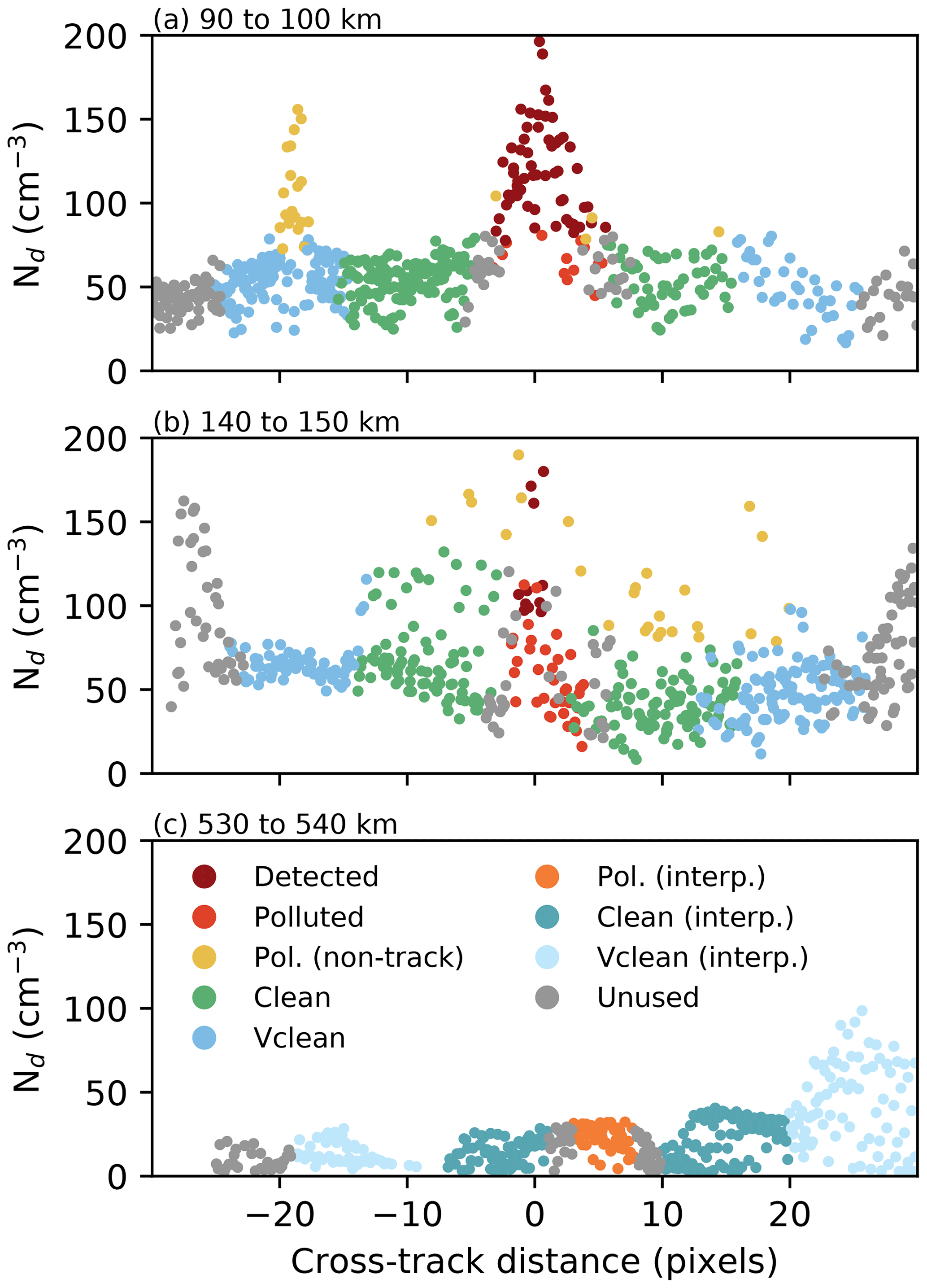
Figure 1Example track chunks and the identification of polluted pixels along the track shown in Fig. 2. Marker colours are shown in (c). Distances in the titles are from the ship location at the time of the satellite overpass. “Detected” pixels are those located by the Segrin et al. (2007) algorithm. “Polluted” pixels are added to the in-ship-track region by the modifications in this work. “Polluted (non-track)” pixels were detected, but removed from the ship track region in this work. The “clean” pixels are used as an unperturbed control situation, while “vclean” is a further control. The interpolated pixels (c) are from segments where no detected pixels exist. Further details are in the text.
With a buffer region of two pixels (>2 km), corresponding clean/control regions are identified at 10 pixels to either side of the track and “vclean” regions at a further 10 pixels to either side of the polluted region. Distances are in pixels to keep an approximately similar number of pixels in each region for each segment. The clean and vclean regions exclude the polluted (non-track) pixels, as nearby ship tracks (as shown in Fig. 1a) are not representative of the background cloud state. This may not always be the correct decision, as crossing ship tracks (Fig. 1b) may be more representative of the background, but it has little impact on the results presented in this work.
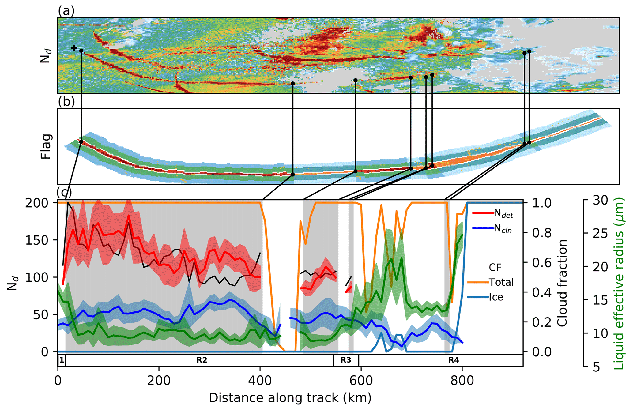
Figure 2An example ship track. (a) The Nd field from MODIS; grey regions indicate no liquid cloud. The ship position is marked with a cross and the dot markers are to identify regions of the ship track. (b) Pixels as identified by the ship track algorithm. Red regions are polluted regions of the ship track and green regions are the corresponding clean regions. Orange regions are interpolated ship track locations based on the identified polluted regions as described in the text. Blue regions are the corresponding unperturbed regions for the interpolated ship track locations. (c) The change in properties along the ship track. Grey regions are “detected” ship track segments (polluted pixels are identified) and the black lines connect the edges of these regions between subplots. The R2 region along the bottom shows the section of the track identified by a human from the day microphysics imagery. Note that these do not have to overlap. Red is Npol for regions where the ship track is detected and blue Ncln with the shaded regions showing the standard deviation within that segment. The thin black line is the Nd enhancement, εN (). The unperturbed re and standard deviation are shown in green. The total CF is in orange and the ice CF in light blue.
The classifications are then aggregated into 15 min (10 km) segments. This is a short enough time period to allow the initial development of the track to be resolved and these two measures are approximately equal for relative wind speed of 40 km h−1 (Durkee et al., 2000a). A full 20 h ship track classification is shown in Fig. 2b, with the flag colours following Fig. 1. Only 20 175 segments (out of 96 720 total) contain detected pixels. To identify polluted pixels in segments where there are no detected pixels, the width from the nearest segment with a detected pixel is interpolated along the estimated emissions trajectory (even within the hand-identified region (R2 in Fig. 2c)).
Cloud properties are recorded along the length of the ship track for both polluted pixels and the corresponding clean/control region outside the track (Fig. 2c). The Nd for polluted (red; Npol) and unperturbed (blue; Ncln) regions is calculated following the method of Quaas et al. (2006), applying the filtering as outlined in Grosvenor et al. (2018). In this example, there is a general decrease in Nd along the length of the ship track, but with a considerable fluctuation. The detected Nd enhancement factor (thin black line; ) shows a much smoother decrease, as it incorporates correlated fluctuations in Npol and Ncln.
The retrieved cloud properties in this work are from the MODIS Aqua collection 6.1 cloud product (MYD06L2; Platnick et al., 2017) and the meteorological properties are from the ERA5 reanalysis. Supplemental information about the background aerosol comes from the sulfate concentration in the MERRA reanalysis following McCoy et al. (2017).
The uncertainties throughout this work are calculated using a bootstrap method (Efron, 1979) with 1000 samples and are shown with a 16 %–84 % uncertainty range. This range is chosen such that significance at an individual time between high and low SOx is indicated by the non-overlap of these ranges.
2.3 Potential radiative forcing
To compare the radiative effect of ship tracks in different conditions, a potential radiative forcing (PRF) is calculated following Eq. (1). This is not the true radiative forcing of the ship track, as it ignores diurnal variations in the cloud response to aerosol and incoming solar flux (F↓; approximated by a constant 280 Wm−2).
The PRF is calculated for each segment individually, with A denoting the area of the polluted region within the segment. The cloud albedo (α) is calculated from the cloud optical depth (τ) following Eq. (2) (Bohren, 1987). The surface ocean albedo is taken as a constant 0.04 (a representative value from Jin et al., 2004). Only liquid clouds are considered in the CF (derived from “Cloud_Phase_Optical_Properties”). The impact of CF changes is calculated by setting CFpol=CFcln to exclude the impact of CF adjustments.
The results from this work are split into two sections; the first deals with the macrophysical properties of the ship track (length, width, detectability, CF), whereas the second focuses on the microphysical properties and the liquid water path.
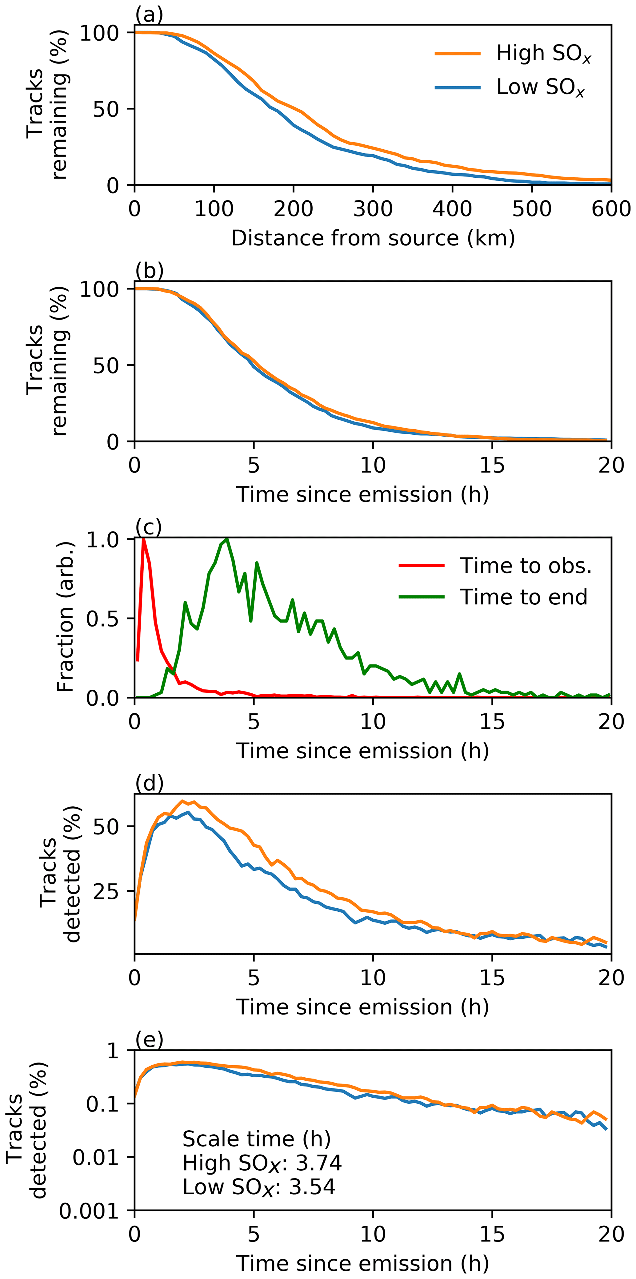
Figure 3(a) Track length (distance to oldest observed segment) for ships with high and low SOx emissions. (b) The same as (a), but using the time since emission instead of the distance. (c) Histograms showing the time to first observation (red) and last observation (green) for the tracks used in this study. (d) The percentage of tracks that are “detected” within any given 15 min segment. Note that this is less than 100 % in many cases due to gaps in ship tracks. (e) as (d) but with a log y axis.
3.1 Macrophysical properties
3.1.1 Track length
The median ship track in this study is last observed at a distance of about 200 km from the source ship, with longer ship tracks more commonly observed behind ships with higher SOx emissions (Fig. 3a). The difference is significantly reduced when using time as a coordinate (Fig. 3b), due to faster ships (producing longer ship tracks) typically burning more fuel and so emitting more SOx. To account for this, we use time since emission as the along-track coordinate throughout the rest of this work.
There is a large variation in the time to initial observation (time to obs.) and the time to last observation for the ship tracks in this work (Fig. 3c). As in previous studies (Durkee et al., 2000a), the mean time to a first observation of the ship track is under an hour, with this database having a mean of 45 min. There is a long tail, with some tracks not being observed until 5 h since emission. These long times before initial observation are due to a lack of cloud at ship locations and the identification of time from distance, rather than decoupling increasing the time to cloud (Liu et al., 2000). A large variation in the length of the observed section of the ship track is also found, with a median length of 5 h but some lasting only an hour and others lasting almost 20. The tracks in this work are on average shorter than those in Durkee et al. (2000a) and Schreier et al. (2007), partially due to differences in the criteria used to select the tracks.
Many of these ship tracks have gaps (segments where the track is not detected). The maximum detected fraction is around 1–2 h after emission, where each 15 min segment has an approximately 60 % chance of containing a detected ship track (Fig. 3d). Although the difference is small, ships with higher SOx emissions produce ship tracks that are more likely to be detected for a longer period of time (Fig. 3d and e). This also suggests that the overall lifetime for the whole population of ship tracks is not a strong function of SOx; ships with larger SOx emissions are more likely to generate tracks that can be detected for a longer period of time and so might be expected to have a larger radiative impact.
3.1.2 Track formation and detection
The majority of segments do not contain a detected track; what limits ship track formation in these segments? For each segment lacking a detected track, four tests are applied in order. T1: is the segment outside a MODIS image (granule)? T2: is there no cloud in the segment? T3: is the segment ice cloud? T4: is the εN less than 1.4 (a 40 % enhancement)? The percentage of segments satisfying these tests are shown in Fig. 4 with the tests applied in order (i.e. segments satisfying T2 are not checked for T3 or T4).
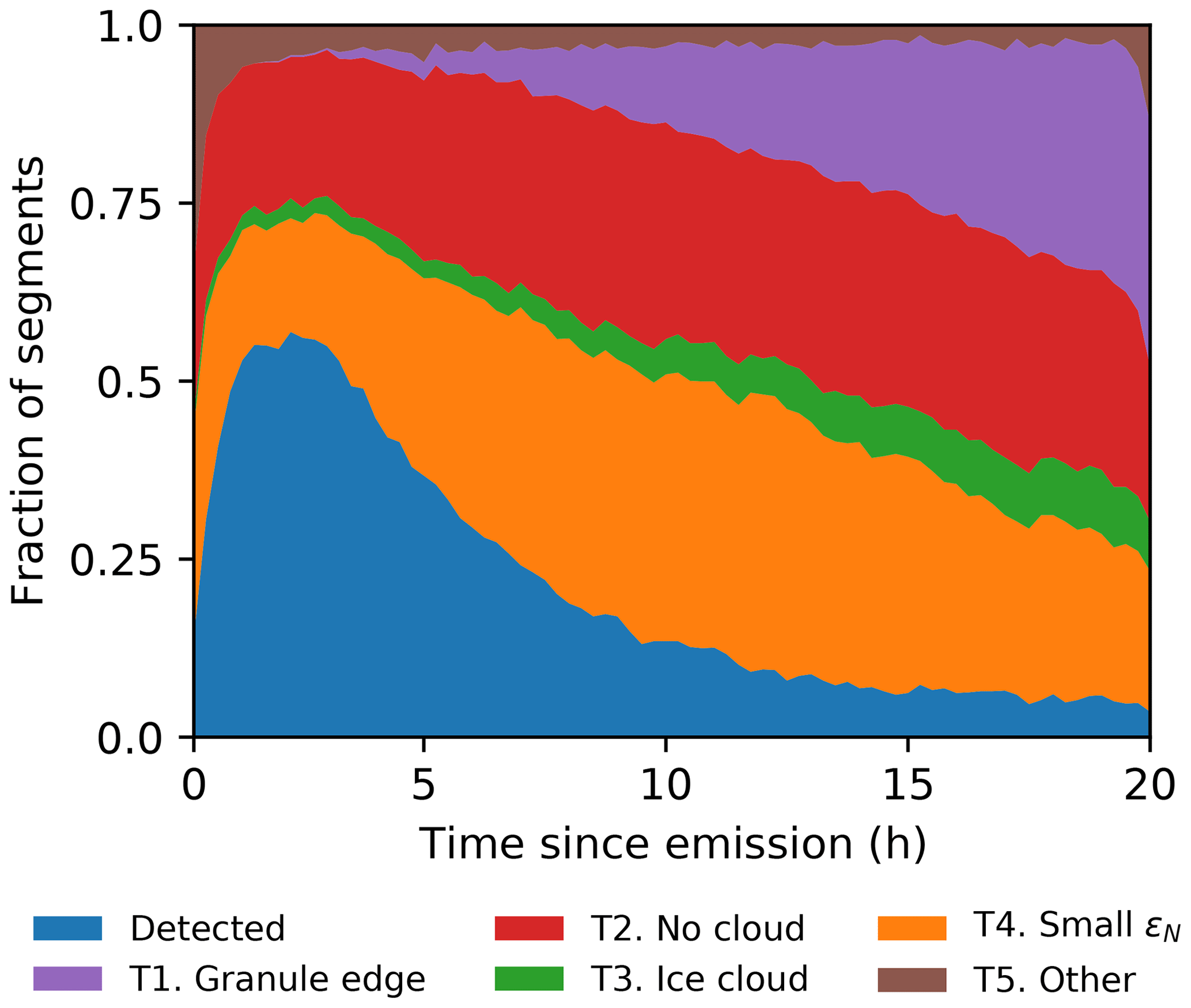
Figure 4Reasons for track non-detection in segments as a function of time since emission. The tests are applied in the order T1–4.
Although many ship tracks are located close to the edge of a MODIS image (“granule”), only a small number of ship tracks disappear because they reach the edge of the MODIS granule. Around 30 % of ship tracks reach a granule edge 20 h after emission. In around 25 % of segments, a lack of cloud prevents the detection of a ship track. This is expected given the CF in this region and is approximately constant with time since emission. Similarly, the small impact of overlying ice cloud on the detection of ship tracks is primarily due to the low ice CF in subtropical subsidence regions.
The impact of a small εN increases with time since emission. Without the individual history of the segments, it is not possible to conclusively separate the dissipation of the ship track from an increased background Nd. The small εN (T4) provides an indication of segments that could potentially form detectable ship tracks with increases in ship SOx emissions, although meteorological conditions will also prevent the formation or observation of ship tracks in some conditions (Noone et al., 2000; Possner et al., 2018; Gryspeerdt et al., 2019b). Even in a region with large amounts of low-level liquid cloud, the frequency of occurrence of liquid cloud is a significant control on the length of ship tracks.
3.1.3 Track widths
Ship track width (defined as the maximum cross-track distance between polluted pixels within a segment) increases gradually with time since emission (Fig. 5a), similar to previous studies (Durkee et al., 2000a). Although the ship track width is highly sensitive to outlier polluted pixels, a weak dependence of width on SOx emissions is observed, with a larger width for higher SOx emissions.
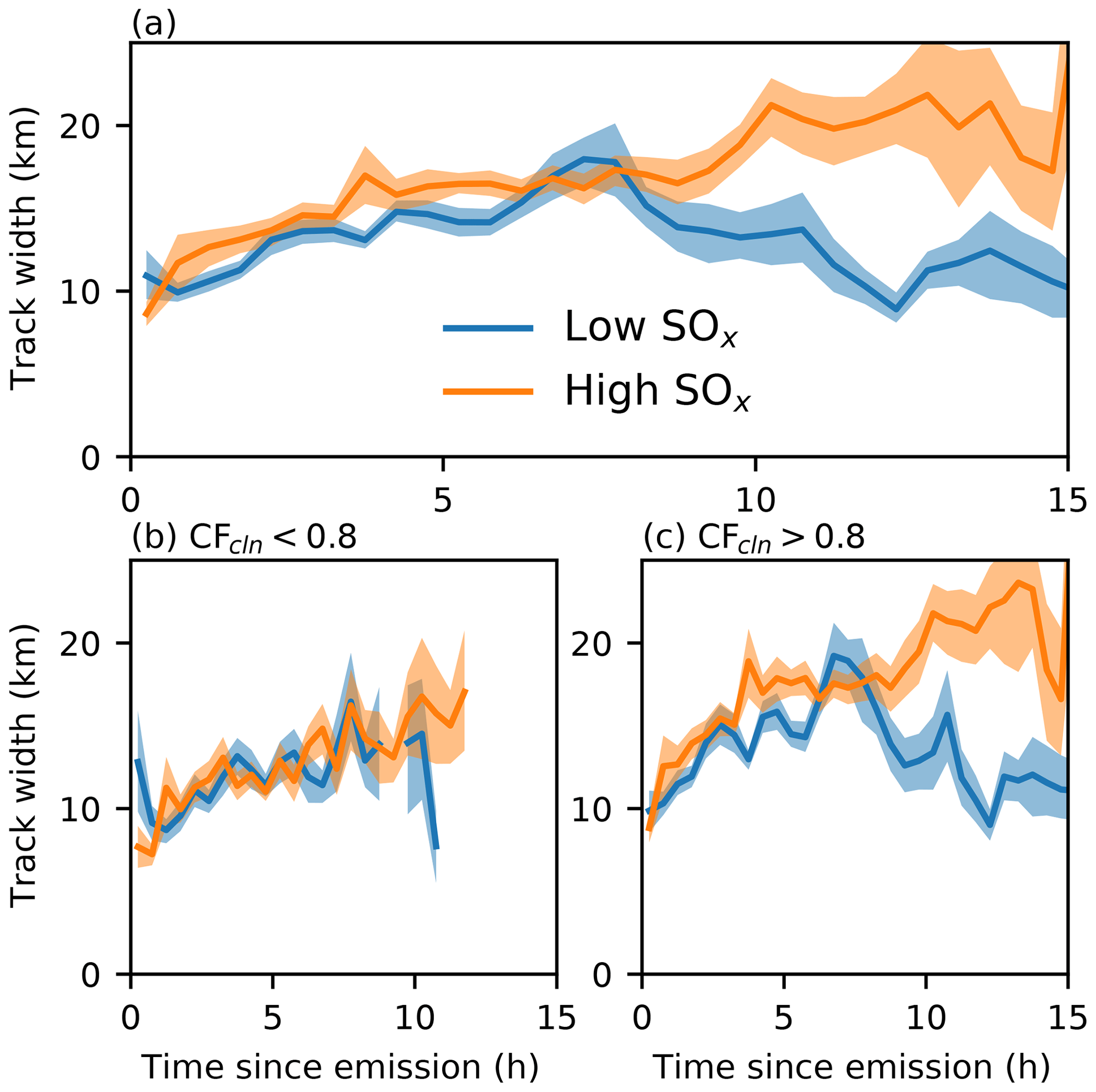
Figure 5(a) Ship track width as a function of time since emission for high (orange) and low (blue) SOx emitting ships. (b) As (a) but only for segments with a CFcln<0.8. (c) As (a) for segments with a CFcln>0.8. Averaged over half-hour periods.
This sensitivity of track width to SOx depends on the background cloud state. Considering only segments with a lower out-of-track CF (CFcln<0.8), the width rises slowly over time but with little sensitivity to the initial aerosol perturbation (Fig. 5b). In contrast, the high CFcln segments have a width that is more sensitive to the ship SOx emissions (Fig. 5c).
Differences in the cloud regimes indicated by CFcln may explain this difference in behaviour. Lower CFcln situations are more likely to be open-celled stratocumulus (Muhlbauer et al., 2014). In this situation, the width of the track is controlled primarily by the cell width, rather than the aerosol perturbation, due to a less efficient mixing of aerosol between cells (Scorer, 1987). Over time, mixing between the cells due to the collapse and creation of new open cells (Feingold et al., 2010) allows the track to widen, gradually affecting a wider region as more cells are included in the track.
The high CFcln situation is more likely to be closed-celled stratocumulus or sea fog (Ackerman et al., 1993). Particularly in the sea-fog case, the lack of a strong cellular structure control on the ship track width allows a dependence on the SOx emissions, with higher SOx emissions creating a wider plume and so a wider initial ship track. The quick and continued growth of the ship track in the first 5 h for these high CFcln cases (Fig. 5c) may be linked to this initial plume dispersion. Similar to the low CFcln case, the gradual growth in the plume over time after this fast-growth period may be linked to cloud processes and mixing. Future model studies will be useful to identify the factors controlling the growth of the ship track width.
3.1.4 Controls on track length
Given the strong impact of cloud occurrence on the disappearance of ship tracks (Fig. 4), factors controlling liquid cloud occurrence will also have an effect on the ship track length. The estimated inversion stability (EIS; Wood and Bretherton, 2006) has a strong link to low cloud cover in this region, but a comparison between high and low EIS environments shows only a 20 % increase in the median lifetime from 5 to 6 h (Fig. 6a). This weak effect is primarily due to the prevalence of short ship tracks in this work and the time-dependent impact of meteorology on ship track lifetime.
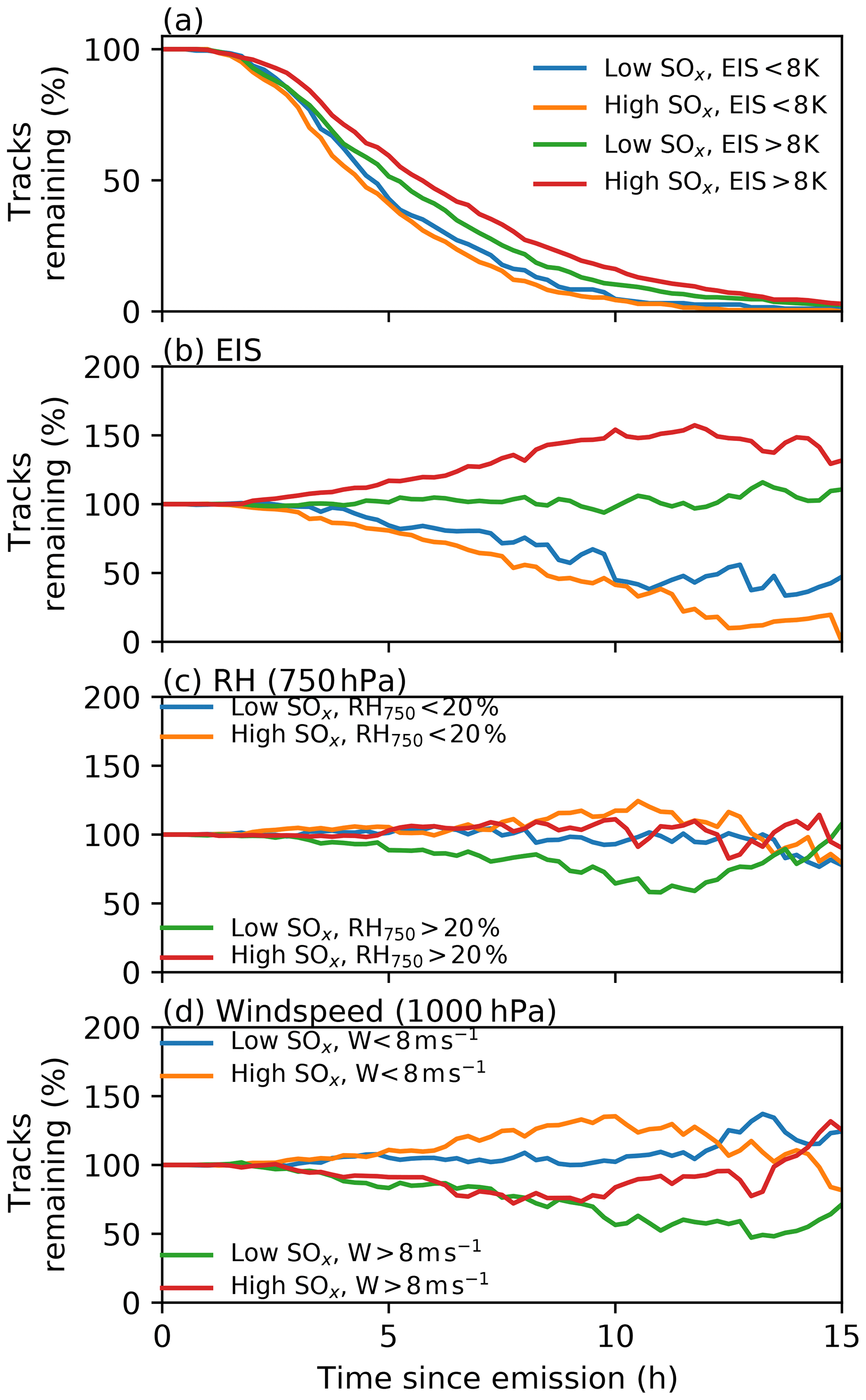
Figure 6Ship track length as function of meteorological parameters. (a) The percentage of tracks remaining for high and low SOx emissions for high and low EIS (averaged along the track). (b) The percentage of tracks remaining as a fraction of the tracks remaining in the total dataset, comparing the impact of emissions at high and low EIS. (c) As (b) but for cloud top relative humidity (750 hPa). (d) As (b) but for high and low 1000 hPa wind speed.
Normalising by the total number of ship tracks remaining in the total sample highlights a much clearer role for meteorology, with ship tracks in low average EIS environments only half as likely to have a lifetime longer than 10 h compared those in a higher EIS environment due to the lower cloud fraction (Fig. 6b). The low cloud fraction also impacts the sensitivity to SOx emissions, with the lifetime of ship tracks in low EIS environments being almost insensitive to SOx emissions. In contrast, the lifetime of high EIS ship tracks is much more sensitive to SOx emissions, as the high CF makes dissipation processes more important. This is supported by studies aiming to produce a climatology of ship tracks finding more ship tracks in regions of extensive low cloud cover (Schreier et al., 2007).
Despite a strong controlling influence on the formation of ship tracks (Gryspeerdt et al., 2019b), cloud top humidity has a much weaker impact on ship track length. Drier cloud tops typically indicate longer ship tracks, perhaps due to an increased in-cloud updraught and so higher sensitivity to aerosol (Lilly, 1968). A slight decrease in ship track length is observed for moister cloud tops.
Wind speed has a stronger influence on ship track length, with higher wind speeds producing shorter ship tracks. Although ship track formation is more common at high wind speeds (Gryspeerdt et al., 2019b), these ship tracks are typically shorter and have a length that is initially less sensitive to the size of the aerosol perturbation. This may be due to a number of factors. Sea salt production is enhanced at high wind speeds, which may lead to a decrease in Nd, perhaps through giant CCN production (Lehahn et al., 2011; Gryspeerdt et al., 2016; McCoy et al., 2017), an increase in precipitation and so a reduction in the impact of the aerosol perturbation.
3.1.5 Cloud fraction enhancement
As well as creating increases in Nd that allow their detection, the ship tracks in this study also have a higher cloud fraction than the control region (Fig. 7). An average increase of around 3 % over the first 10 h is observed, peaking around 3–4 h after emission. The CF increase is not strongly correlated to the ship SOx emissions (Fig. 7a) but varies significantly as a function of the background cloud state. In relatively clean conditions (Ncln<50 cm−3), the CF is increased by almost 10 % within the first 5 h after emission (Fig. 7b). In contrast, the CF in already polluted conditions does not increase significantly inside the ship track (Fig. 7c), partly due to the higher CF found at higher Nd (e.g. Gryspeerdt et al., 2016) restricting the opportunity for any further CF increase within the ship track.
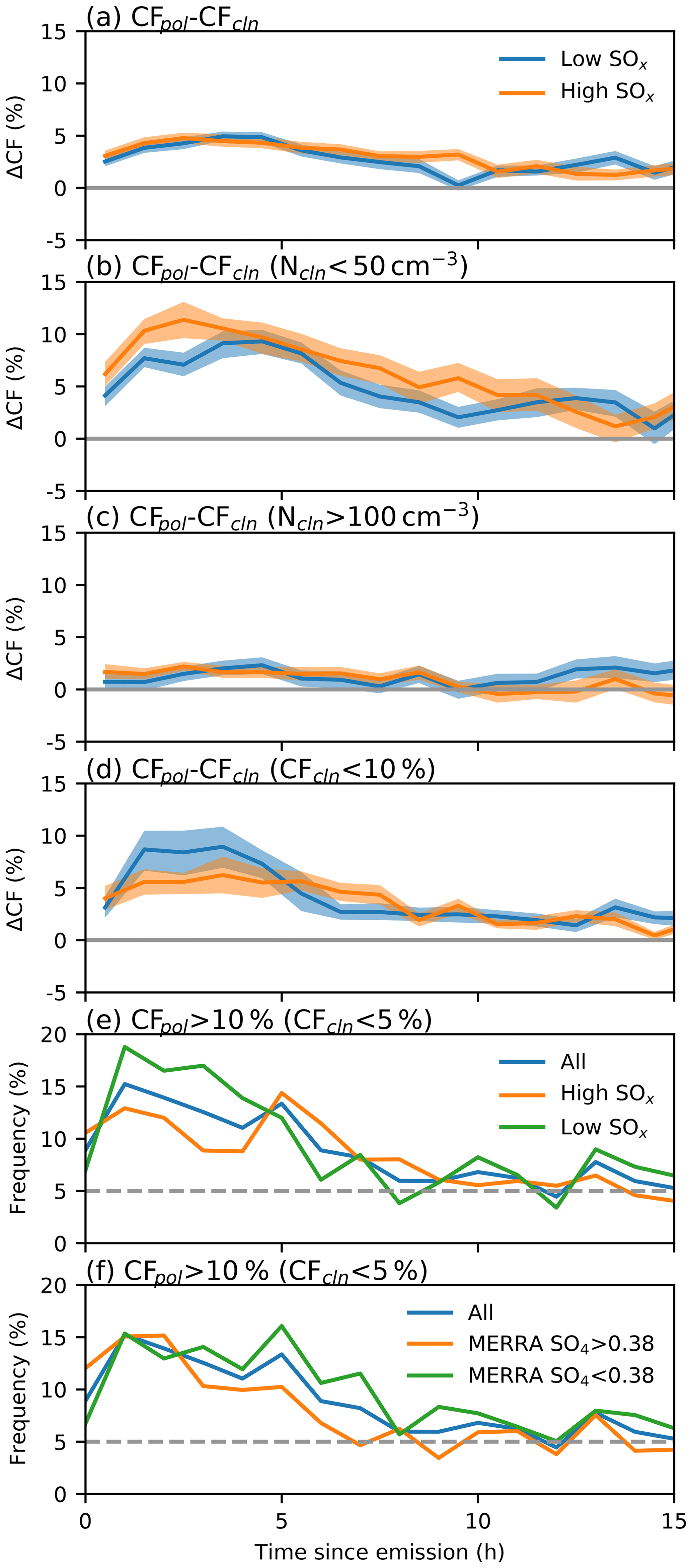
Figure 7(a) Cloud fraction in the polluted ship track regions compared to the corresponding clean locations. (b) As (a) but only for cases where the Nd in the clean region is <50 cm−3. (c) As (a) but only for cases where the Nd in the clean region is >100 cm−3. (d) As (a) but only for cases where the CFcln is <10 %. (e) The percentage of cases with CFpol>10 % and CFcln<5 %, stratified by the ship SOx emissions. (f) As (e) but stratified by background SO4. Grey lines are grid lines.
By estimating the ship aerosol trajectories, ship tracks are located even when there are no surrounding clouds (preventing the detection algorithm from operating). By selecting cases with a low CFcln (<10 %), a 3 %–7 % increase in cloud amount (ΔCF) is found in the early stages of the ship track (Fig. 7d). The ΔCF is concentrated in a small fraction of segments; in the first 5 h of the ship track, of the segments with a CFcln<5 %, only 10 % have a CFpol>10 % (Fig. 7e). A CF increase is more common in cases with lower SOx increases, but does not appear to be correlated to the reanalysis background aerosol (Fig. 7f). These segments with a low CFcln but higher CFpol (Fig. 7e) are potential aerosol-limited CF cases.
By selecting cases with a low CFcln, random biases in the CF will increase ΔCF (as CF cannot be less than 0 %). This gives the appearance of an aerosol-limited CF, increasing the fraction of potentially aerosol-limited cases. As this effect is independent of time since emission, the asymptote to 5 % of potential aerosol-limited cases (>10 h in Fig. 7) provides a simple estimate of this bias. Although this would suggest that up to 5 % of the potentially aerosol-limited cases in the early stages of the ship track development are the result of this bias, it leaves around 5 % of the clear-sky cases as aerosol-limited (Fig. 7e). However, as this estimate relies on gaps in and dissipation of existing ship tracks, more work is required to establish whether it is an accurate measure of aerosol-limited conditions, particularly in regions far from existing clouds.
3.2 Microphysics
The previous section showed that the background meteorological state has a controlling influence on the macrophysical properties of ship tracks and their sensitivity to aerosol. These are not independent from the microphysical properties of the ship track, particularly the εN, which is closely related to ship track detection. Changes in the microphysics can also have a distinct impact on the potential radiative forcing from ship tracks. In this section, the changes in the Nd and LWP are examined to investigate these controls in more depth and quantify the radiative response as a function of time.
3.2.1 Polluted vs. detected
Detected pixels (more than 2 standard deviations above the background Nd) are only a subset of the pixels within the ship track. In this section, the “polluted” Nd (Fig. 1) is used as a measure of the Nd within the ship track, enabling a consistent comparison between segments with and without a detected ship track. The detected εN is positive by definition (Fig. 8a). As it includes (undetected) pixels with a lower Nd, the polluted Nd is smaller than the detected Nd and in some cases can lead to an εN of less than 1 (typically in segments where there are no detected pixels).

Figure 8(a) The Nd enhancement (εN) for detected cases and all polluted cases 2 to 3 h after emission for all cases with sufficient cloud. (b) The relationship between polluted and detected for all cases in (a) where both metrics are derived.
In segments where both the polluted and detected Nd exist, there is a close correlation between the polluted and detected εN (r=0.9; Fig. 8b). This correlation rises further (to 0.95), when only segments with more than five detected pixels are included, indicating that the primary source of uncertainty is in the detected εN. This supports the use of the polluted εN for characterising the ship tracks in this work.
3.2.2 Nd development
Previous studies have shown a strong link between the ship emissions and the detected εN (Gryspeerdt et al., 2019b). This enhancement peaks in the early stages of the ship track formation and decreases quickly with time (Fig. 9a). As it depends on the relatively small number of detected pixels, the uncertainty in the enhancement is relatively high and the difference between the high and low SOx ships becomes small after 5 h. Part of this uncertainty is due to a sampling effect, as weak εN segments have no detected pixels and so are excluded from the calculation. This means that the average enhancement tends towards the lowest detectable enhancement.
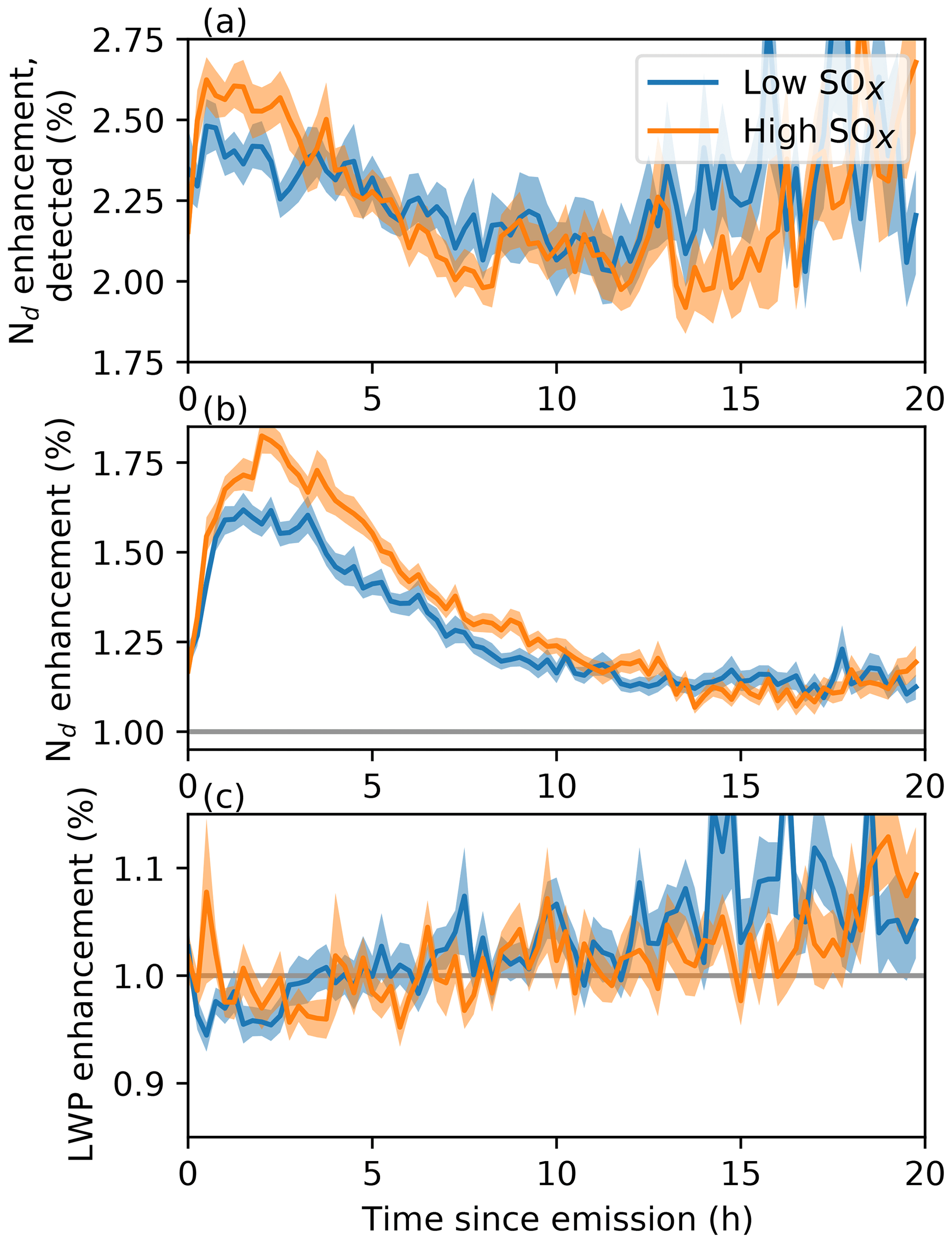
Figure 9(a) The change in εN for detected pixels only as a function of time from emission, for low and high SOx emitting ships respectively. (b) As (a), but including all the pixels within the ship track as the polluted pixels. (c) As (b), but for the LWP instead of the Nd.
A clearer signal is found using the polluted εN (Fig. 9b). Following a quick increase in εN during the ship track formation, a maximum is reached within about 1 h (similar to the formation timescale in Fig. 3c). This timescale is longer than the formation timescale for the detected εN (Fig. 9a), as the detected εN only includes clouds where the ship SOx emissions have already had a detectable impact. The polluted εN is almost 50 % larger for ships with higher SOx emissions (>0.13 kg s−1) than lower emissions, a difference maintained until more than 10 h since emission. The decrease in εN with time emphasises the importance of temporal development when considering aerosol impacts on clouds, especially those from an isolated aerosol source where there is no replenishment of the aerosol. This also demonstrates that if time since emission is not accounted for, the εN (detected or polluted) is not a good measure of the aerosol perturbation.
Although noisy, some patterns can be observed in the LWP enhancement (; Fig. 9c). There is an initial decrease of approximately 5 % in the εL, followed by an increase in the εL after 2 h, becoming positive (increased LWP inside the ship track) at around 7 h since emission. There is no clear difference in εL between ships with high and low SOx emissions.
3.2.3 Meteorology and Nd development
As well as being a clear function of time, the εN is also a function of meteorological state, such that even the εN at a given time since emission is not necessarily a good measure of the aerosol perturbation. As the meteorological conditions can change along the length of a ship track, the results in the following sections are composited, with the meteorological conditions being calculated independently for each segment along the track. This allows situations where a track transects a region of variable meteorological conditions to be investigated.

Figure 10As Fig. 9b, but stratified by: (a, b) estimated inversion strength (EIS), (c, d) relative humidity at 750 hPa, and (e, f) 1000 hPa wind speed. Orange and blue are high and low SOx emissions respectively.
The εN is higher at low EIS (Fig. 10a), where it is also sensitive to ship SOx emissions with increased SOx enhancing the εN further. However, the εN for both the high and low SOx tracks becomes very similar after 4 h. This is similar to the track length in Fig. 6b, which is also not a strong function of the aerosol perturbation. In both cases, the impact of meteorological variations dominates the variability from the magnitude of the aerosol perturbation. In contrast, while the εN is smaller (partially due to a larger Ncln; Bennartz and Rausch, 2017) in the high EIS cases (Fig. 10b), the signal from the aerosol perturbation remains to almost 20 h (although the εN itself is still a strong function of time).
Relative humidity also affects εN, with ship tracks at lower cloud top humidity being more sensitive to the initial aerosol perturbation (Fig. 10c). When the cloud top humidity is higher, the sensitivity of the εN to the aerosol perturbation disappears almost entirely (Fig. 10d). This is expected following previous work showing ship tracks are more likely to form in regions with a low cloud top humidity (Gryspeerdt et al., 2019b), potentially due to the increased cloud top cooling promoting strong updraughts and so a larger sensitivity to aerosol (Lilly, 1968).
The dependence of the εN development on surface wind speed may have a similar origin. The larger sensitivity of εN to the aerosol perturbation at higher wind speeds (Fig. 10f) may be due to the increased surface fluxes promoting a larger in-cloud updraught and hence a more aerosol-limited environment.
3.2.4 LWP sensitivity
The impact of aerosol on the liquid water path is often quantified as the sensitivity of LWP to Nd, (e.g. Han et al., 2002; Feingold, 2003). This sensitivity can be calculated directly from a ship track, comparing the polluted and corresponding clean regions, and has been used to quantify the strength of LWP adjustments to aerosol (e.g. Toll et al., 2019). However, the temporal development in εL and εN (Figs. 9b and c) will generate a negative bias to the Nd–LWP sensitivity if the time since emission is not accounted for (Fig. 11). This negative relationship is driven primarily by the different timescales of the LWP and Nd response and could occur even if the aerosol produced a strong LWP increase, highlighting the difficulties of using εN as a measure of the aerosol perturbation without accounting for the temporal development of the perturbation.
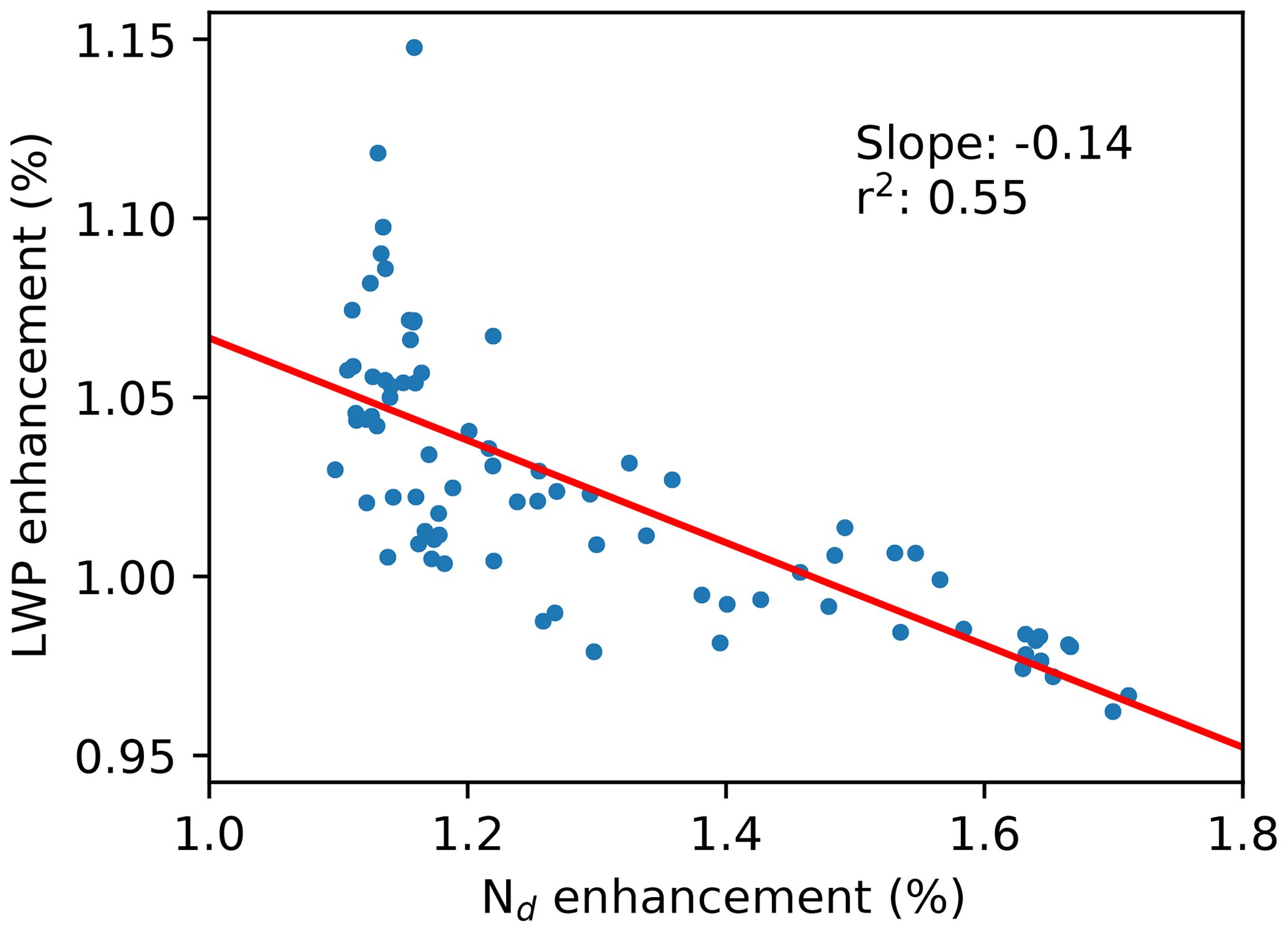
Figure 11The relationship between the mean LWP and Nd enhancements in Fig. 9. The slope and r2 values for a linear regression are given in the plot.

Figure 12The LWP sensitivity to Nd as a function of time since emission. Panels (a) and (b) show the development of the sensitivity as a function of Ncln and as a function of RH(750 hPa) respectively. The blue line is the same in both plots as a reference. Linear fits for the data from 2 to 10 h after emission, along with a standard error on the fit, are also shown.
To include this development, the average sensitivity (calculated individually for each segment using the εL and polluted εN) is shown as function of time from emission in Fig. 12a. Considering all the ship tracks together (blue line), the sensitivity almost instantaneously decreases to −0.1 before slowly decreasing to −0.2 over the following 15 h. Using Ncln as a measure of the background cloud state (e.g. Gryspeerdt et al., 2019b), it is seen that not only is the sensitivity a function of time since emission, it is a strong function of Ncln (Fig. 12a). A bi-directional LWP response has been observed in several previous studies (Han et al., 2002; Chen et al., 2012; Gryspeerdt et al., 2019a; Toll et al., 2019) and hypothesised to be a combination of precipitation suppression (generating a positive sensitivity of LWP to Nd) and aerosol dependent entrainment (generating a negative sensitivity; Ackerman et al., 2004).
This bi-directional LWP sensitivity response is clear in (Fig. 12a). For both the clean and polluted background clouds, the sensitivity is initially very similar, then begins to diverge after 2 h and produce a more positive sensitivity in cleaner background conditions. This is consistent with the precipitation suppression effect that dominates in clean regions, but the enhanced entrainment is more important for polluted situations (e.g. Gryspeerdt et al., 2019a). This behaviour continues to at least 20 h since emission, although the sensitivities at long timescales should be treated with some caution due to the small number of ship tracks remaining after such long times. The exact values of the sensitivity at large times since emission also depend significantly on the choices made in the ship track pixel identification algorithm, although the qualitative results remain. At long timescales, the sensitivity would tend towards large-scale statistics, which may be impacted by retrieval biases from correlated errors in the LWP and Nd retrievals (Gryspeerdt et al., 2019a).
A similar divergence in the sensitivity is observed as a function of cloud top humidity (Fig. 12b). Both dry and moist cloud-top conditions maintain a similar sensitivity for the first 4 h; at subsequent times, the more humid cloud tops have a more positive sensitivity, increasing over time. This is consistent with the impact of humidity through cloud top entrainment shown in previous studies (Ackerman et al., 2004; Toll et al., 2019).
While these results support those found in previous studies, there are a number of important factors that must be taken into account when interpreting those studies. First, as demonstrated in model studies (Glassmeier et al., 2021), the Nd–LWP sensitivity is not constant with time. This introduces extra uncertainties into studies that do not account for this variation. Second, εN is a poor indicator of the aerosol perturbation under some meteorological conditions (Fig. 10). If the εN is primarily a factor of the local meteorology, this increases the potential impact of meteorological covariations on the sensitivity (e.g. Gryspeerdt et al., 2019a). Finally, the timescales involved may hint at the potential for a retrieval bias creating an extra negative sensitivity in these results (see Sect. 4.2).
3.2.5 LWP development
By averaging the changes in LWP over hour-long periods, the temporal changes in LWP after the aerosol emission become clearer (Fig. 13). A decrease in LWP is observed at short timescales, followed by an increase in LWP at longer timescales (Wang and Feingold, 2009b). There is no clear difference in LWP evolution for the high or low SOx emissions.
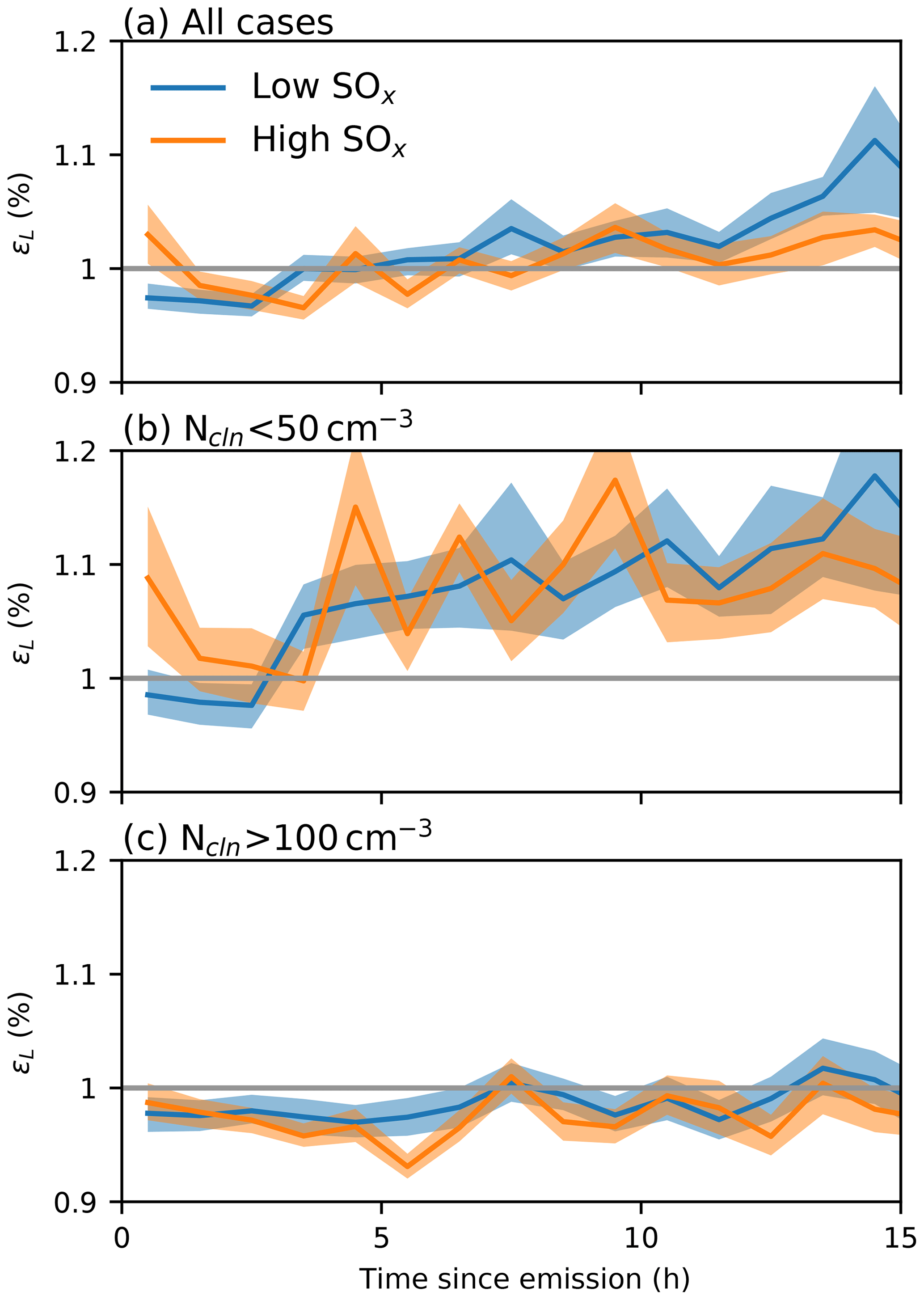
Figure 13Development of LWP along ship tracks for (a) all ships, (b) clean background environments (Ncln<50 cm−3) and (c) polluted background environments (Ncln>100 cm−3).
As seen in the sensitivity, when looking at cases with a clean background (Fig. 13b), after a short-term decrease in LWP, there is a strong increase in LWP after 5 h since emission. This is likely due to precipitation suppression and the circulation adjustments created around a spatially limited aerosol perturbation (Scorer, 1987; Wang and Feingold, 2009b), particularly in an open-celled stratocumulus regime (Christensen and Stephens, 2011).
For ship tracks forming in polluted environments, there is a small decrease in LWP (Fig. 13c). This decrease is larger for ship tracks formed by larger SOx emissions, although the overall magnitude of the effect is smaller than the increase in cleaner conditions. Although the sensitivity appears to continue to increase, the near constant εL (Fig. 13c) appears to suggest that the increase in sensitivity is almost exactly offset by the decrease in εN. This is in contrast to the results from (Glassmeier et al., 2021), which suggests that the change in sensitivity comes from the LWP adjusting to the change in Nd. Further work is required to properly understand to what extent ship tracks and the response to isolated pollution sources represent the actual response of cloud and particularly LWP to aerosol perturbations.
4.1 Potential radiative forcing
The combination of these increases in Nd (Fig. 10), LWP (Fig. 13) and CF (Fig. 7) produce an increase in reflected shortwave radiation, providing a way to compare the different perturbations with a similar metric. Integrating the potential radiative forcing along each ship track before creating a composite shows that about half the total radiative impact of the composite ship track comes in the first 5 h (Fig. 14a). During this period, the SOx emissions of the ship do not have a strong impact on the integrated forcing. The SOx impact increases in the later stages of the ship track lifetime, where higher SOx emitting ships produce a larger εN (Fig. 9b) later in their lifetimes. Excluding the CF change (Fig. 14d) shows that approximately half the total radiative effect of the ship track comes from CF increases. The weak correlation of these CF increases to the ship SOx emissions explains the insensitivity of the integrated forcing to SOx during the early stages of the track.
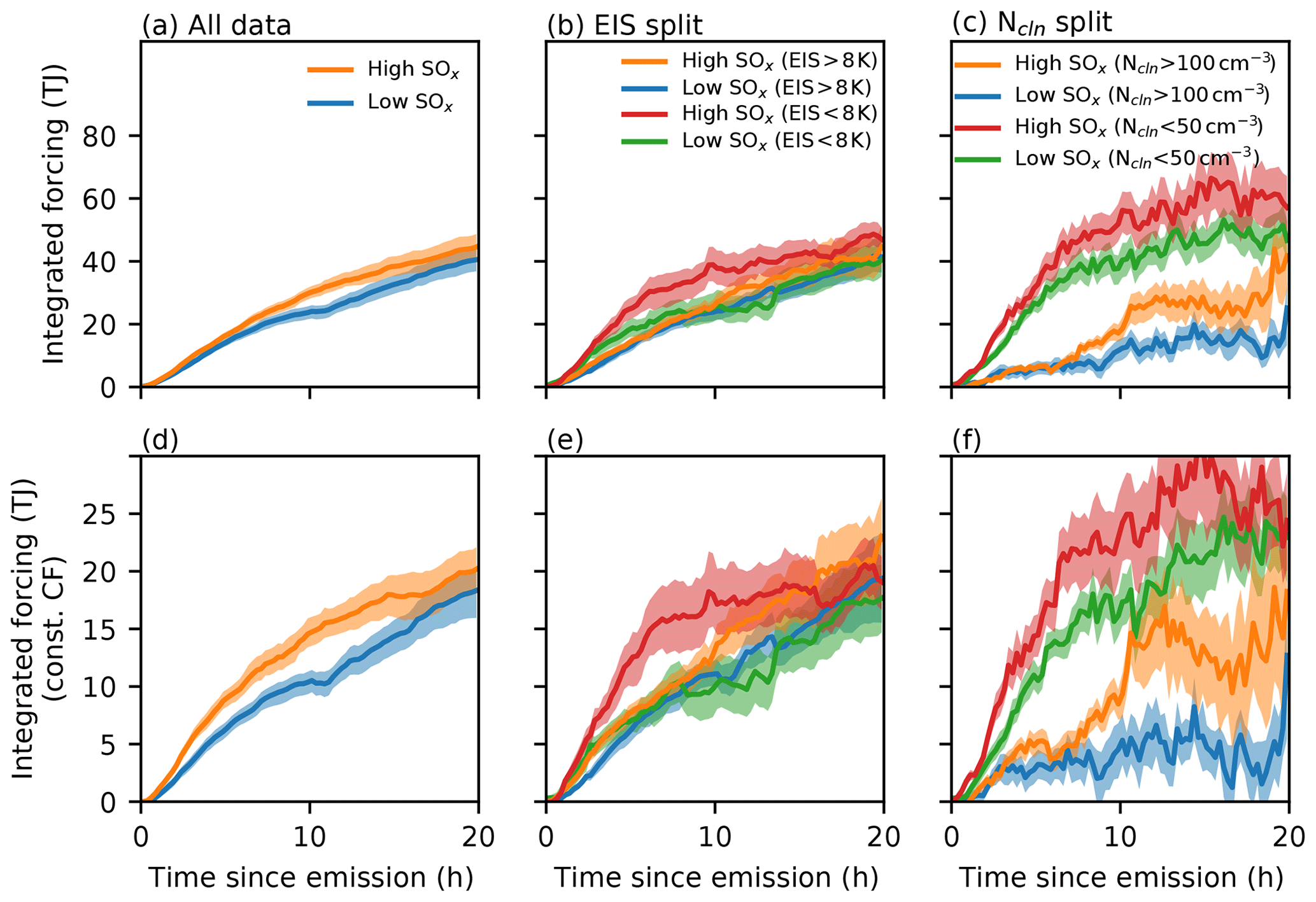
Figure 14The integrated potential forcing as a function of time since emission including (top row) and excluding (bottom row) CF changes (Eq. 1). Note the different scales. (a, d) All ship tracks, separated by high and low SOx emissions. (b, e) Separated by high and low SOx emissions for high EIS (>8 K; orange and blue) and low EIS (<8 K, red and green as high and low SOx respectively). (c, f) As (b) and (e), but for high Ncln (>100 cm−3; orange and blue) and low Ncln (<50 cm−3; red and green).
The liquid cloud fraction has previously been shown to be the primary control on ship track formation (Gryspeerdt et al., 2019b). This is strongly linked to the EIS, with more liquid cloud in more stable environments (Wood and Bretherton, 2006). However, despite a higher cloud fraction at high EIS, ship tracks formed in lower EIS environments have a larger radiative effect (Fig. 14b). This is partly due to the lower CF allowing the CF (and hence forcing) to increase within the ship track. With a higher background CF, there is less scope for a forcing due to a CF increase (Goren et al., 2019). This interpretation is supported by the results at a constant cloud fraction (Fig. 14e), where after an initial difference in the forcing (due to the higher εN at low EIS; Fig. 10), the integrated forcing for the high and low EIS populations is very similar after 10 h.
Although EIS has some control over the radiative effect of ship tracks, background Nd have the largest impact on ship track radiative properties (Fig. 14c), with larger εN (Gryspeerdt et al., 2019b), εL (Fig. 13) and CF enhancement (Fig. 7) occurring with a clean background. The forcing for the clean background (Ncln<50 cm−3) cases is mostly within the first 7 h, with very little increase in the integrated forcing after this time. This is likely due to the lower cloud fraction at a lower Ncln (Gryspeerdt et al., 2016) both enhancing the forcing from CF increases in the early stages of the track and limiting the forcing from εN increases in the later stages. In contrast, the integrated forcing from ship tracks in polluted backgrounds shows a relatively steady increase with time, although after 20 h it still has less than half the integrated forcing of the ship tracks in clean environments. These ship track locations were only estimated up to 20 h from emission. Some very long-lived ship tracks have radiative impacts lasting several days (Goren and Rosenfeld, 2012), which would lead to significant changes at longer timescales.
4.2 Timescales
The Nd response to the aerosol perturbation proceeds at a timescale approximating a boundary layer mixing timescale of around half an hour (Figs. 3d and 9). The timescale for the precipitation suppression impact on LWP to become clear is around 2 h (Fig. 12a). This increase in LWP is quicker than the 4 h delay in Wang and Feingold (2009b) but slower than the almost instantaneous LWP response to a Nd increase in Feingold et al. (2015). It may also indicate that the LWP response to precipitation or circulation effects is faster than model simulations suggest.
The aerosol impact through a modification of entrainment proceeds at a slower pace. In Fig. 12b, it takes more than 4 h for the impact of variations in cloud top humidity to begin to appear. As the impact of cloud top entrainment depends on the humidity, the timescale for humidity variations to impact the Nd–LWP sensitivity is the relevant timescale for the impact of aerosol-dependent entrainment. This compares well with the results from Glassmeier et al. (2021), which shows a characteristic timescale for the LWP adjustment via entrainment of 20 h, which produces a 20 % of the total change after 4 h.
While these timescales match previous work, the Nd–LWP sensitivity adjusts almost immediately behind the ship (Fig. 12). The sensitivity reaches −0.1 within the first 15 min, meaning that the LWP has changed on the same timescale as the Nd. While the Nd can respond at this timescale (e.g. Wang and Feingold, 2009b), LWP adjustments depending on precipitation or entrainment appear to operate at longer timescales (Fig. 12). An increased droplet surface area and thus condensation rate could produce a fast change to the LWP but would lead to LWP increases (Koren et al., 2014).
An re retrieval bias may also be the cause of this near instant LWP adjustment. Both the LWP and Nd are calculated using the cloud optical depth and re , so random errors in the re become correlated errors in the LWP and Nd, generating a negative sensitivity bias (e.g. Gryspeerdt et al., 2019a). Retrieval biases are insensitive to the time since emission and so would be capable of producing this almost instant LWP adjustment.
One potential cause of an re retrieval bias could be in the droplet size distribution (DSD) (Painemal and Zuidema, 2011). The shape of the DSD affects the relative number of small and large droplets and hence the link between the Nd and re. Aircraft studies have shown a wider DSD in ship tracks compared to the surrounding cloud, which would create an uncertainty in retrieval of cloud properties in ship tracks (Noone et al., 2000). Future high spatial-resolution polarimeters may be able to resolve this ambiguity.
If the initial value of the sensitivity of −0.1 represents the impact of retrieval biases, this suggests the negative sensitivities determined from previous studies of ship tracks should be smaller, resulting in a weaker LWP reduction in response to aerosol. Recent studies have suggested that the LWP adjustments inferred from ship tracks may be underestimated due to the lack of consideration of the ship track temporal development (Glassmeier et al., 2021). These model results are supported by the observational evidence presented in this work (Fig. 12), suggesting that the long-term LWP sensitivity to Nd may be larger than found in previous studies. It should be noted that the long-term temporal development of these ship tracks (particularly those that contain no detected pixels), will tend to the large-scale statistics, which themselves may be subject to biases from correlated errors (e.g. Gryspeerdt et al., 2019a). However, these two factors suggest that the interpretation of current and future studies inferring LWP adjustments from natural experiments should consider the temporal development of the perturbation and the possibility of retrieval errors.
4.3 Future improvements
This work has shown that many ship track properties vary significantly along the length of the track. As ship tracks do not transmit information along their length, they can be considered a collection of semi-independent segments, with the same initial aerosol perturbation, but at different times since emission. Using the ship location and the local wind field for reanalysis, the time since emission is inferred, allowing the timescales of the relevant cloud and aerosol processes to be measured. However, the results in this work come with some caveats.
The MODIS images are still only a snapshot of the cloud field, such that the time axis determined from the ship and cloud motion is not a real time axis. The unperturbed clouds will also develop over the time period (Christensen et al., 2009; Kabatas et al., 2013), such that the “unperturbed” clouds here are not a true measure of the cloud at the time of the aerosol perturbation. The polluted clouds will also have evolved, not necessarily in the same manner. The climatological meteorological fields also affect both the clean and polluted clouds (15 h can be several hundred kilometres). This generates uncertainties that will be resolved in future work through the use of geostationary observations.
Although many ship tracks are intersected by CloudSat/CALIPSO, it is not enough to build up a picture of the precipitation development in these ship tracks. MODIS views every segment in each track; with 1209 tracks, almost 100 000 segments are used in this study. CloudSat will typically only view one segment per track (if any), so that resolving the development to the same detail requires 80 times as many ship tracks. Expanding this work to a global scale will not only allow the inclusion of other regions for ship track formation (Schreier et al., 2007) but will enable a more complete picture of the factors limiting and controlling aerosol perturbations on cloud properties.
This study uses Nd to locate ship tracks, in contrast to earlier work that used near-IR reflectance (e.g. Segrin et al., 2007). This increases the contrast and hence detectability of ship tracks in cloud-covered scenes and cases where there is no change in re (see Supplement). This comes at a cost of a reduced ship track detection efficiency in scenes with low numbers of successful liquid cloud retrievals. A more effective combination of the information from these two sources would lead to a more complete sample of ship tracks in a wide variety of background conditions.
Cloud responses to aerosol perturbations are not instant but instead develop over characteristic timescales. This work uses ship position information and reanalysis wind fields to develop a time axis for satellite-observed ship tracks, providing a method for measuring the timescales of aerosol–cloud interactions from individual satellite images. The advected emission locations also provide an estimate for ship track locations in regions where they are too weak to be detected by existing methods (Fig. 2).
While ships with higher SOx emissions typically produce longer ship tracks, the median lifetime of the ship tracks studied in this work is not a strong function of the ship emissions (Fig. 3). The role of ship emissions for ship track length varies by meteorological background, with shorter ship tracks being found in more unstable (higher EIS environments), where the ship track length is insensitive to the ship SOx emissions (Fig. 6b). In contrast, higher SOx emissions lead to a significant increase in track lifetime in more stable environments, due to the higher cloud fraction and stronger role for dissipation. Across their lifetime, a lack of cloud and insufficient Nd perturbations have approximately an equal role in ship track disappearance (Fig. 4).
After an initial increase in track width (within the first 5 h), track width is relatively insensitive to the time since emission (Fig. 5). In high CF environments (an indicator of closed cells or sea fog), the track width increases with SOx emissions. In low CF environments (indicating open cells), the track width is largely independent of SOx, as the track width is largely controlled by the cell width (Scorer, 1987).
The reanalysis wind field is used to locate ship tracks in otherwise cloud-free environments (Fig. 7). A significant increase in CF is found during the first 10 h of the ship track lifetime, suggesting that around 5 % of clear-sky cases in this region are aerosol-limited (Fig. 7e). There is a large uncertainty on this number, due to potential random fluctuations in the cloud fraction retrievals. Further studies are required to establish the extent of these aerosol-limited cases across the global oceans.
The microphysical properties of the ship track, particularly the Nd enhancement (εN) along with the LWP enhancement, also vary significantly with time since emission (Fig. 9). The εN quickly reaches a maximum around an hour after emission, before slowly decreasing. The strength of the εN maximum and its sensitivity to SOx depend on the meteorological state, although cases with the largest εN (such as at low EIS; Fig. 10a) often have a lower sensitivity to the SOx emissions (such as when the cloud top relative humidity is larger than 20 %). The εN sensitivity to SOx can persist over several hours. In high EIS situations, ship tracks produced by high SOx ships still have a larger εN after 10 h (Fig. 10b).
While the εN is correlated to SOx in some cases, it is not a good measure of the aerosol perturbation, especially if the time since emission is not accounted for. The LWP enhancement (εL) increases over time (Fig. 9), such that εN and LWP temporal development create a negative Nd–LWP sensitivity in ship tracks, even if aerosols produced an increase in LWP (Fig. 11). Even when accounting for the ship track development, the Nd–LWP sensitivity remains strongly dependent on the time since emission, along with the background cloud and meteorological state (Fig. 12). After 2 h, positive sensitivities become visible in clean cases and a dependence on the cloud top humidity appears after around 4 h. These timescales are related to cloud processes (e.g. Feingold et al., 2015; Glassmeier et al., 2021), but the near-instant appearance of the negative sensitivity (within 15 min; Fig. 12) hints at a potential retrieval error. Correlated errors in the Nd and LWP retrievals is one possible explanation, perhaps caused by a change in the shape of the droplet size distribution (Noone et al., 2000), although in situ studies are required to investigate this possibility. This temporal development of the Nd–LWP should be accounted for in studies of cloud adjustment to aerosol.
When combined, the radiative impact of the ship tracks investigated in this work is concentrated in the first 5–10 h after emission (Fig. 14), with approximately half of the overall effect being due to the increase in CF in the early stages of the ship track lifetime. This emphasises the large potential role of cloud fraction adjustments to the overall potential radiative forcing (Goren and Rosenfeld, 2014). This strong impact of the CF increase means that ship tracks in lower EIS environments have a higher potential radiative forcing (Fig. 14b), although the background Nd dominates, with ship tracks in clean environments producing a 4 times larger integrated radiative forcing over the 20 h study period.
Although uncertainties remain, this study demonstrates how isolated aerosol perturbations can be used to measure the timescales of aerosol impacts on cloud properties, showing that the Nd perturbation is not often a good measure of the size of the aerosol perturbation and that meteorology and background cloud state have an important role in determining the sensitivity of cloud properties to aerosol. Together, the results in this work emphasise the importance of accounting for time when using observations of isolated aerosol perturbations to constrain aerosol–cloud interactions.
Ship emissions were derived from location data from exactEarth. MODIS data used in this work were acquired from Level-1 and Atmosphere Archive and Distribution System (LAADS) Distributed Active Archive Center (DAAC), located in the Goddard Space Flight Center in Greenbelt, Maryland, USA (https://ladsweb.nascom.nasa.gov/, last access: 20 April 2021) (NASA, 2012). The code used in this work can be obtained from the lead author.
The supplement related to this article is available online at: https://doi.org/10.5194/acp-21-6093-2021-supplement.
EG designed the study and performed the analysis. TS and TG assisted with the interpretation of the results. All authors provided comments and suggestions on the manuscript.
The authors declare that they have no conflict of interest.
The authors would like to thank the reviewers for their helpful comments on the manuscript.
This research has been supported by a Royal Society University Research Fellowship (grant no. URF/R1/191602) and the European Research Council, H2020 grant no. 821205 (FORCeS).
This paper was edited by Zhanqing Li and reviewed by Kentaroh Suzuki and one anonymous referee.
Ackerman, A. S., Toon, O. B., and Hobbs, P. V.: Dissipation of Marine Stratiform Clouds and Collapse of the Marine Boundary Layer Due to the Depletion of Cloud Condensation Nuclei by Clouds, Science, 262, 226–229, https://doi.org/10.1126/science.262.5131.226, 1993. a
Ackerman, A. S., Kirkpatrick, M. P., Stevens, D. E., and Toon, O. B.: The impact of humidity above stratiform clouds on indirect aerosol climate forcing, Nature, 432, 1014, https://doi.org/10.1038/nature03174, 2004. a, b, c
Albrecht, B. A.: Aerosols, Cloud Microphysics, and Fractional Cloudiness, Science, 245, 1227–1230, https://doi.org/10.1126/science.245.4923.1227, 1989. a
Bennartz, R. and Rausch, J.: Global and regional estimates of warm cloud droplet number concentration based on 13 years of AQUA-MODIS observations, Atmos. Chem. Phys., 17, 9815–9836, https://doi.org/10.5194/acp-17-9815-2017, 2017. a
Bohren, C. F.: Multiple scattering of light and some of its observable consequences, Am. J. Phys., 55, 524, https://doi.org/10.1119/1.15109, 1987. a
Boucher, O., Randall, D. A., Artaxo, P., Bretherton, C., Feingold, G., Forster, P. M., Kerminen, V.-M., Kondo, Y., Liao, H., Lohmann, U., Rasch, P., Satheesh, S. K., Sherwood, S., Stevens, B., and Zhang, X. Y.: Clouds and Aerosols, Cambridge University Press, Cambridge, https://doi.org/10.1017/CBO9781107415324.016, 2013. a
Bretherton, C. S., Blossey, P. N., and Uchida, J.: Cloud droplet sedimentation, entrainment efficiency, and subtropical stratocumulus albedo, Geophys. Res. Lett., 34, L03813, https://doi.org/10.1029/2006GL027648, 2007. a
Chen, Y.-C., Christensen, M. W., Xue, L., Sorooshian, A., Stephens, G. L., Rasmussen, R. M., and Seinfeld, J. H.: Occurrence of lower cloud albedo in ship tracks, Atmos. Chem. Phys., 12, 8223–8235, https://doi.org/10.5194/acp-12-8223-2012, 2012. a
Christensen, M. W. and Stephens, G. L.: Microphysical and macrophysical responses of marine stratocumulus polluted by underlying ships: Evidence of cloud deepening, J. Geophys. Res., 116, D03 201, https://doi.org/10.1029/2010JD014638, 2011. a
Christensen, M. W., Coakley, J. A., and Tahnk, W. R.: Morning-to-Afternoon Evolution of Marine Stratus Polluted by Underlying Ships: Implications for the Relative Lifetimes of Polluted and Unpolluted Clouds, J. Atmos. Sci., 66, 2097–2106, https://doi.org/10.1175/2009JAS2951.1, 2009. a, b
Christensen, M. W., Jones, W. K., and Stier, P.: Aerosols enhance cloud lifetime and brightness along the stratus-to-cumulus transition, P. Natl. Acad. Sci. USA, 117, 17591–17598, https://doi.org/10.1073/pnas.1921231117, 2020. a
Conover, J. H.: Anomalous Cloud Lines, J. Atmos. Sci., 23, 778–785, https://doi.org/10.1175/1520-0469(1966)023<0778:ACL>2.0.CO;2, 1966. a
Durkee, P. A., Chartier, R. E., Brown, A., Trehubenko, E. J., Rogerson, S. D., Skupniewicz, C., Nielsen, K. E., Platnick, S., and King, M. D.: Composite Ship Track Characteristics, J. Atmos. Sci., 57, 2542–2553, https://doi.org/10.1175/1520-0469(2000)057<2542:CSTC>2.0.CO;2, 2000a. a, b, c, d
Durkee, P. A., Noone, K. J., Ferek, R. J., Johnson, D. W., Taylor, J. P., Garrett, T. J., Hobbs, P. V., Hudson, J. G., Bretherton, C. S., Innis, G., Frick, G. M., Hoppel, W. A., O'Dowd, C. D., Russell, L. M., Gasparovic, R., Nielsen, K. E., Tessmer, S. A., Öström, E., Osborne, S. R., Flagan, R. C., Seinfeld, J. H., and Rand, H.: The Impact of Ship-Produced Aerosols on the Microstructure and Albedo of Warm Marine Stratocumulus Clouds: A Test of MAST Hypotheses 1i and 1ii., J. Atmos. Sci., 57, 2554–2569, https://doi.org/10.1175/1520-0469(2000)057<2554:TIOSPA>2.0.CO;2, 2000b. a
Efron, B.: Bootstrap methods: Another look at the jackknife, Ann. Stat., 7, 1–26, 1979. a
Feingold, G.: First measurements of the Twomey indirect effect using ground-based remote sensors, Geophys. Res. Lett., 30, 1287, https://doi.org/10.1029/2002GL016633, 2003. a
Feingold, G., Koren, I., Wang, H., Xue, H., and Brewer, W. A.: Precipitation-generated oscillations in open cellular cloud fields, Nature, 466, 849–852, https://doi.org/10.1038/nature09314, 2010. a
Feingold, G., Koren, I., Yamaguchi, T., and Kazil, J.: On the reversibility of transitions between closed and open cellular convection, Atmos. Chem. Phys., 15, 7351–7367, https://doi.org/10.5194/acp-15-7351-2015, 2015. a, b
Glassmeier, F., Hoffmann, F., Johnson, J. S., Yamaguchi, T., Carslaw, K. S., and Feingold, G.: Aerosol-cloud-climate cooling overestimated by ship-track data, Science, 371, 485–489, https://doi.org/10.1126/science.abd3980, 2021. a, b, c, d, e, f
Goren, T. and Rosenfeld, D.: Satellite observations of ship emission induced transitions from broken to closed cell marine stratocumulus over large areas, J. Geophys. Res., 117, 17206, https://doi.org/10.1029/2012JD017981, 2012. a, b, c
Goren, T. and Rosenfeld, D.: Decomposing aerosol cloud radiative effects into cloud cover, liquid water path and Twomey components in marine stratocumulus, Atmos. Res., 138, 378–393, https://doi.org/10.1016/j.atmosres.2013.12.008, 2014. a
Goren, T., Kazil, J., Hoffmann, F., Yamaguchi, T., and Feingold, G.: Anthropogenic Air Pollution Delays Marine Stratocumulus Breakup to Open Cells, Geophys. Res. Lett., 46, 14135–14144, https://doi.org/10.1029/2019GL085412, 2019. a
Grosvenor, D. P., Sourdeval, O., Zuidema, P., Ackerman, A., Alexandrov, M. D., Bennartz, R., Boers, R., Cairns, B., Chiu, J. C., Christensen, M., Deneke, H., Diamond, M., Feingold, G., Fridlind, A., Hünerbein, A., Knist, C., Kollias, P., Marshak, A., McCoy, D., Merk, D., Painemal, D., Rausch, J., Rosenfeld, D., Russchenberg, H., Seifert, P., Sinclair, K., Stier, P., van Diedenhoven, B., Wendisch, M., Werner, F., Wood, R., Zhang, Z., and Quaas, J.: Remote Sensing of Droplet Number Concentration in Warm Clouds: A Review of the Current State of Knowledge and Perspectives, Rev. Geophys., 56, 409–453, https://doi.org/10.1029/2017RG000593, 2018. a
Gryspeerdt, E., Stier, P., and Partridge, D. G.: Satellite observations of cloud regime development: the role of aerosol processes, Atmos. Chem. Phys., 14, 1141–1158, https://doi.org/10.5194/acp-14-1141-2014, 2014. a
Gryspeerdt, E., Quaas, J., and Bellouin, N.: Constraining the aerosol influence on cloud fraction, J. Geophys. Res., 121, 3566–3583, https://doi.org/10.1002/2015JD023744, 2016. a, b, c, d
Gryspeerdt, E., Goren, T., Sourdeval, O., Quaas, J., Mülmenstädt, J., Dipu, S., Unglaub, C., Gettelman, A., and Christensen, M.: Constraining the aerosol influence on cloud liquid water path, Atmos. Chem. Phys., 19, 5331–5347, https://doi.org/10.5194/acp-19-5331-2019, 2019a. a, b, c, d, e, f
Gryspeerdt, E., Smith, T. W. P., O'Keeffe, E., Christensen, M. W., and Goldsworth, F. W.: The Impact of Ship Emission Controls Recorded by Cloud Properties, Geophys. Res. Lett., 46, 12547–12555, https://doi.org/10.1029/2019GL084700, 2019b. a, b, c, d, e, f, g, h, i, j, k, l, m
Han, Q., Rossow, W. B., Zeng, J., and Welch, R.: Three Different Behaviors of Liquid Water Path of Water Clouds in Aerosol–Cloud Interactions, J. Atmos. Sci., 59, 726–735, https://doi.org/10.1175/1520-0469(2002)059<0726:TDBOLW>2.0.CO;2, 2002. a, b
Jin, Z., Charlock, T. P., Smith, W. L., and Rutledge, K.: A parameterization of ocean surface albedo, Geophys. Res. Lett., 31, L22301, https://doi.org/10.1029/2004GL021180, 2004. a
Kabatas, B., Menzel, W. P., Bilgili, A., and Gumley, L. E.: Comparing Ship-Track Droplet Sizes Inferred fromTerra and Aqua MODIS Data, J. Appl. Meteorol. Clim., 52, 230–241, https://doi.org/10.1175/JAMC-D-11-0232.1, 2013. a, b, c
Koren, I., Feingold, G., and Remer, L. A.: The invigoration of deep convective clouds over the Atlantic: aerosol effect, meteorology or retrieval artifact?, Atmos. Chem. Phys., 10, 8855–8872, https://doi.org/10.5194/acp-10-8855-2010, 2010. a
Koren, I., Dagan, G., and Altaratz, O.: From aerosol-limited to invigoration of warm convective clouds, Science, 344, 1143–1146, https://doi.org/10.1126/science.1252595, 2014. a
Lehahn, Y., Koren, I., Altaratz, O., and Kostinski, A. B.: Effect of coarse marine aerosols on stratocumulus clouds, Geophys. Res. Lett., 38, L20 804, https://doi.org/10.1029/2011GL048504, 2011. a
Lensky, I. M. and Rosenfeld, D.: Clouds-Aerosols-Precipitation Satellite Analysis Tool (CAPSAT), Atmos. Chem. Phys., 8, 6739–6753, https://doi.org/10.5194/acp-8-6739-2008, 2008. a
Lilly, D. K.: Models of cloud-topped mixed layers under a strong inversion, Q. J. Roy. Meteor. Soc., 94, 292–309, https://doi.org/10.1002/qj.49709440106, 1968. a, b
Liu, Q., Kogan, Y. L., Lilly, D. K., Johnson, D. W., Innis, G. E., Durkee, P. A., and Nielsen, K. E.: Modeling of Ship Effluent Transport and Its Sensitivity to Boundary Layer Structure, J. Atmos. Sci., 57, 2779–2791, https://doi.org/10.1175/1520-0469(2000)057<2779:MOSETA>2.0.CO;2, 2000. a
Matsui, T., Masunaga, H., Kreidenweis, S. M., Pielke, R. A., Tao, W.-K., Chin, M., and Kaufman, Y. J.: Satellite-based assessment of marine low cloud variability associated with aerosol, atmospheric stability, and the diurnal cycle, J. Geophys. Res., 111, 17204, https://doi.org/10.1029/2005JD006097, 2006. a
McCoy, D. T., Bender, F. A.-M., Mohrmann, J. K. C., Hartmann, D. L., Wood, R., and Grosvenor, D. P.: The global aerosol–cloud first indirect effect estimated using MODIS, MERRA, and AeroCom, J. Geophys. Res., 122, 1779–1796, https://doi.org/10.1002/2016JD026141, 2017. a, b
McCoy, D. T., Field, P., Gordon, H., Elsaesser, G. S., and Grosvenor, D. P.: Untangling causality in midlatitude aerosol–cloud adjustments, Atmos. Chem. Phys., 20, 4085–4103, https://doi.org/10.5194/acp-20-4085-2020, 2020. a
Meskhidze, N., Remer, L. A., Platnick, S., Negrón Juárez, R., Lichtenberger, A. M., and Aiyyer, A. R.: Exploring the differences in cloud properties observed by the Terra and Aqua MODIS Sensors, Atmos. Chem. Phys., 9, 3461–3475, https://doi.org/10.5194/acp-9-3461-2009, 2009. a
Muhlbauer, A., Ackerman, T. P., Comstock, J. M., Diskin, G. S., Evans, S. M., Lawson, R. P., and Marchand, R. T.: Impact of large-scale dynamics on the microphysical properties of midlatitude cirrus, J. Geophys. Res., 119, 3976–3996, https://doi.org/10.1002/2013JD020035, 2014. a
NASA: LAADS DAAC, available at: https://ladsweb.nascom.nasa.gov/, last access: 20 April 2021. a
Noone, K. J., Johnson, D. W., Taylor, J. P., Ferek, R. J., Garrett, T., Hobbs, P. V., Durkee, P. A., Nielsen, K., Öström, E., O'Dowd, C., Smith, M. H., Russell, L. M., Flagan, R. C., Seinfeld, J. H., de, B. L., van, G. R. E., Hudson, J. G., Brooks, I., Gasparovic, R. F., and Pockalny, R. A.: A Case Study of Ship Track Formation in a Polluted Marine Boundary Layer., J. Atmos. Sci., 57, 2748, https://doi.org/10.1175/1520-0469(2000)057<2748:ACSOST>2.0.CO;2, 2000. a, b, c
Painemal, D. and Zuidema, P.: Assessment of MODIS cloud effective radius and optical thickness retrievals over the Southeast Pacific with VOCALS-REx in situ measurements, J. Geophys. Res., 116, D24 206, https://doi.org/10.1029/2011JD016155, 2011. a
Platnick, S., Meyer, K. G., King, M. D., Wind, G., Amarasinghe, N., Marchant, B., Arnold, G. T., Zhang, Z., Hubanks, P. A., Holz, R. E., Yang, P., Ridgway, W. L., and Riedi, J.: The MODIS Cloud Optical and Microphysical Products: Collection 6 Updates and Examples From Terra and Aqua, IEEE T. Geosci. Remote, 55, 502–525, https://doi.org/10.1109/TGRS.2016.2610522, 2017. a
Possner, A., Wang, H., Wood, R., Caldeira, K., and Ackerman, T. P.: The efficacy of aerosol–cloud radiative perturbations from near-surface emissions in deep open-cell stratocumuli, Atmos. Chem. Phys., 18, 17475–17488, https://doi.org/10.5194/acp-18-17475-2018, 2018. a
Quaas, J., Boucher, O., and Lohmann, U.: Constraining the total aerosol indirect effect in the LMDZ and ECHAM4 GCMs using MODIS satellite data, Atmos. Chem. Phys., 6, 947–955, https://doi.org/10.5194/acp-6-947-2006, 2006. a, b
Quaas, J., Stevens, B., Stier, P., and Lohmann, U.: Interpreting the cloud cover – aerosol optical depth relationship found in satellite data using a general circulation model, Atmos. Chem. Phys., 10, 6129–6135, https://doi.org/10.5194/acp-10-6129-2010, 2010. a
Rosenfeld, D., Kaufman, Y. J., and Koren, I.: Switching cloud cover and dynamical regimes from open to closed Benard cells in response to the suppression of precipitation by aerosols, Atmos. Chem. Phys., 6, 2503–2511, https://doi.org/10.5194/acp-6-2503-2006, 2006. a
Rosenzweig, M. R. and Wolpin, K. I.: Natural “Natural Experiments” in Economics, J. Econ. Lit., 38, 827–874, https://doi.org/10.1257/jel.38.4.827, 2000. a
Schreier, M., Mannstein, H., Eyring, V., and Bovensmann, H.: Global ship track distribution and radiative forcing from 1 year of AATSR data, Geophys. Res. Lett., 34, 17814, https://doi.org/10.1029/2007GL030664, 2007. a, b, c
Scorer, R.: Ship trails, Atmos. Environ., 21, 1417–1425, https://doi.org/10.1016/0004-6981(67)90089-3, 1987. a, b, c
Segrin, M. S., Coakley, J. A., and Tahnk, W. R.: MODIS Observations of Ship Tracks in Summertime Stratus off the West Coast of the United States, J. Atmos. Sci., 64, 4330, https://doi.org/10.1175/2007JAS2308.1, 2007. a, b, c, d
Seifert, A., Heus, T., Pincus, R., and Stevens, B.: Large-eddy simulation of the transient and near-equilibrium behavior of precipitating shallow convection, J. Adv. Model. Earth Sy., 7, 1918–1937, https://doi.org/10.1002/2015MS000489, 2015. a
Smith, T. W. P., Jalkanen, J. P., Anderson, B. A., Corbett, J. J., Faber, J., Hanayama, S., O'Keeffe, E., Parker, S., Johansson, L., Aldous, L., Raucci, C., Traut, M., Ettinger, S., Nelissen, D., Lee, D. S., Ng, S., Agrawal, A., Winebrake, J. J., Hoen, M., Chesworth, S., and Pandey, A.: The Third IMO GHG Study, International Maritime Organization (IMO), London, UK, 2015. a, b
Toll, V., Christensen, M., Quaas, J., and Bellouin, N.: Weak average liquid-cloud-water response to anthropogenic aerosols, Nature, 572, 51–55, https://doi.org/10.1038/s41586-019-1423-9, 2019. a, b, c, d
Twomey, S.: Pollution and the planetary albedo, Atmos. Environ., 8, 1251–1256, https://doi.org/10.1016/0004-6981(74)90004-3, 1974. a
Wang, H. and Feingold, G.: Modeling Mesoscale Cellular Structures and Drizzle in Marine Stratocumulus. Part I: Impact of Drizzle on the Formation and Evolution of Open Cells, J. Atmos. Sci., 66, 3237–3256, https://doi.org/10.1175/2009JAS3022.1, 2009a. a
Wang, H. and Feingold, G.: Modeling Mesoscale Cellular Structures and Drizzle in Marine Stratocumulus. Part II: The Microphysics and Dynamics of the Boundary Region between Open and Closed Cells, J. Atmos. Sci., 66, 3257–3275, https://doi.org/10.1175/2009JAS3120.1, 2009b. a, b, c, d
Wood, R. and Bretherton, C. S.: On the Relationship between Stratiform Low Cloud Cover and Lower-Tropospheric Stability, J. Clim., 19, 6425–6432, https://doi.org/10.1175/JCLI3988.1, 2006. a, b
Xue, H. and Feingold, G.: Large-Eddy Simulations of Trade Wind Cumuli: Investigation of Aerosol Indirect Effects, J. Atmos. Sci., 63, 1605–1622, https://doi.org/10.1175/JAS3706.1, 2006. a