the Creative Commons Attribution 4.0 License.
the Creative Commons Attribution 4.0 License.
 | 19 Apr 2021
Ozone variability induced by synoptic weather patterns in warm seasons of 2014–2018 over the Yangtze River Delta region, China
Da Gao
Tijian Wang
Chaoqun Ma
Haokun Bai
Xing Chen
Mengmeng Li
Bingliang Zhuang
Shu Li
Ozone (O3) pollution is of great concern in the Yangtze River Delta (YRD) region of China, and the regional O3 pollution is closely associated with dominant weather systems. With a focus on the warm seasons (April–September) from 2014 to 2018, we quantitatively analyze the characteristics of O3 variations over the YRD, the impacts of large-scale and synoptic-scale circulations on the O3 variations and the associated meteorological controlling factors, based on observed ground-level O3 and meteorological data. Our analysis suggests an increasing trend of the regional mean O3 concentration in the YRD at 1.8 ppb per year over 2014–2018. Spatially, the empirical orthogonal function analysis suggests the dominant mode accounting for 65.7 % variation in O3, implying that an increase in O3 is the dominant tendency in the entire YRD region. Meteorology is estimated to increase the regional mean O3 concentration by 3.1 ppb at most from 2014 to 2018. In particular, relative humidity (RH) plays the most important role in modulating the inter-annual O3 variation, followed by solar radiation (SR) and low cloud cover (LCC). As atmospheric circulations can affect local meteorological factors and O3 levels, we identify five dominant synoptic weather patterns (SWPs) in the warm seasons in the YRD using the t-mode principal component analysis classification. The typical weather systems of SWPs include the western Pacific Subtropical High (WPSH) under SWP1, a continental high and the Aleutian low under SWP2, an extratropical cyclone under SWP3, a southern low pressure and WPSH under SWP4 and the north China anticyclone under SWP5. The variations of the five SWPs are all favorable to the increase in O3 concentrations over 2014–2018. However, crucial meteorological factors leading to increases in O3 concentrations are different under different SWPs. These factors are identified as significant decreases in RH and increases in SR under SWP1, 4 and 5, significant decreases in RH, increases in SR and air temperature (T2) under SWP2 and significant decreases in RH under SWP3. Under SWP1, 4 and 5, significant decreases in RH and increases in SR are predominantly caused by the WPSH weakening under SWP1, the southern low pressure weakening under SWP4 and the north China anticyclone weakening under SWP5. Under SWP2, significant decreases in RH, increases in SR and T2 are mainly produced by the Aleutian low extending southward and a continental high weakening. Under SWP3, significant decreases in RH are mainly induced by an extratropical cyclone strengthening. These changes in atmospheric circulations prevent the water vapor in the southern and northern sea from being transported to the YRD and result in RH significantly decreasing under each SWP. In addition, strengthened descending motions (behind the strengthening trough and in front of the strengthening ridge) lead to decreases in LCC and significant increases in SR under SWP1, 2, 4 and 5. The significant increases in T2 would be due to weakening cold flow introduced by a weakening continental high. Most importantly, the changes in the SWP intensity can make large variations in meteorological factors and contribute more to the O3 inter-annual variation than the changes in the SWP frequency. Finally, we reconstruct an empirical orthogonal function (EOF) mode 1 time series that is highly correlated with the original O3 time series, and the reconstructed time series performs well in defining the change in SWP intensity according to the unique feature under each of the SWPs.
- Article
(13711 KB) - Full-text XML
-
Supplement
(994 KB) - BibTeX
- EndNote


As an air pollutant, surface ozone (O3) is harmful to human health and vegetation growth, such as by damaging human lungs (Jerrett et al., 2009; Day et al., 2017) and destroying forest and agricultural crops (Yue et al., 2017). After the emission control following the “13th Comprehensive Work Plan for Energy Saving and Emission Reduction in China” since 2016, concentrations of many pollutants have decreased over the past few years in China but not of O3. Furthermore, heavy O3 pollution episodes occur more frequently and more severely in China than in Japan, South Korea, the United States and European countries (Lu et al., 2018). Li et al. (2019) proposed that the rapid decrease of fine particulate matter (PM) in China is a reason for such O3 increase as aerosol sinks of hydroperoxy radicals are reduced. Yet, meteorological influences on the O3 increase are unclear and require further investigations.
Surface O3 is mainly formed through complex and nonlinear photochemical reactions of volatile organic compounds (VOCs) and nitrogen oxides (NOx) exposed to the sunlight (Xie et al., 2014). Meteorology can affect O3 levels through modulation of photochemical reactions, advection, convection and turbulent transport, as well as dry and wet depositions (Xie et al., 2016a, b). Synoptic weather patterns (SWPs) and the associated meteorological conditions can impact long-term and daily O3 variations (Hegarty et al., 2007; Santurtun et al., 2015; Gao et al., 2020; Shu et al., 2020). Understanding the mechanisms of meteorological influences on O3 variations and quantifying such influences would help to understand the formation of O3 pollution.
Previous studies have revealed that severe O3 pollution episodes are usually accompanied by high temperature, strong solar radiation, drying conditions and stagnant weather (Jacob and Winner, 2009; Doherty et al., 2013; Shu et al., 2016; Pu et al., 2017; Zhang et al., 2018), and these local meteorological conditions are often related to specific synoptic-scale and large-scale atmospheric circulation systems (Fiore et al., 2003; Leibensperger et al., 2008; Barnes and Fiore, 2013; Shu et al., 2016; Wang et al., 2017; Zhao and Wang, 2017). For example, O3 pollution in the eastern United States is notably influenced by the cyclone frequency (Leibensperger et al., 2008), the latitude of the polar jet over eastern North America (Barnes and Fiore, 2013) and the behavior of the quasi-permanent Bermuda High (Fiore et al., 2003; Wang et al., 2017). In China, Yang et al. (2014) illustrated that the changes in meteorological variables, associated with the East Asian summer monsoon, lead to 2 %–5 % inter-annual variations in surface O3 concentrations over central-eastern China. Zhao and Wang (2017) found that a significantly strong western Pacific subtropical high (WPSH) could result in higher relative humidity (RH), more clouds, more rainfall and less ultraviolet radiation, finally leading to less O3 formation. Using model simulation, Shu et al. (2016) investigated the synergistical impact of the WPSH and typhoons on O3 pollution in the Yangtze River Delta region.
As is known, a region is influenced by different weather systems. Weather classification, as a way to distinguish the different large-scale and synoptic-scale atmospheric circulation systems, is widely used in exploring connections between weather patterns and O3 levels (Han et al., 2020; Gao et al., 2020). Gao et al. (2020) discussed influences of six SWPs on O3 levels in the YRD and revealed differences in O3 pollution levels due to minor changes in atmospheric circulations. However, it is uncertain how changes in the SWPs could lead to O3 pollution in detail, especially in the YRD. For northern China and the Pearl River Delta (PRD) region, Liu et al. (2019) quantified the impact of synoptic circulation patterns on O3 variability in northern China from April to October during 2013–2017. Yang et al. (2019) quantitatively assessed the impacts of meteorological factors and the precursor emissions on the long-term trend of ambient O3 over the PRD region. However, whether variations in SWPs have led to O3 increases in recent years over the YRD has not been sufficiently addressed.
Due to the recent increases in O3 level over the YRD (Gao et al., 2017; Xie et al., 2017), studies on characterizing the O3 variation in the region and understanding the mechanisms for the variation are urgently required. To this end, the temporal and spatial variations in surface O3 including 5-year trend over the YRD are quantitatively investigated, and the mechanisms of meteorological influences on the O3 variations are analyzed. In particular, the characteristics of the corresponding SWPs are discussed in detail. The remainder of this paper is organized as follows. Data and methods are introduced in Sect. 2. The inter-annual variation and 5-year trend and spatial variation characteristics of surface ozone in the YRD are illustrated in Sect. 3.1. The impact of meteorological factors on the O3 variation is discussed in Sect. 3.2. The main SWPs and the effects of their changes on the O3 variation are described in Sect. 3.3. Section 3.4 discusses the contributions of the changes in SWP intensity and frequency to the inter-annual variation and trend of O3. Finally, conclusions and discussions are shown in Sect. 4.
2.1 O3 and meteorological datasets
The maximum daily 8 h average O3 data are available from the National Environmental Monitoring Center of China and were acquired from the air quality real-time publishing platform (http://106.37.208.233:20035, last access: 15 April 2021). The hourly observation data of meteorological factors including air temperature (T2), RH and wind speed (WS) in the warm seasons from April to September over 2014–2018 were acquired from the National Meteorological Center of China Meteorological Administration (http://www.wmc-bj.net, last access: 15 April 2021). A total of 26 cities are selected as typical cities representative of the YRD according to the “Yangtze River Delta Urban Agglomeration Development Plan” approved by China's State Council in 2016. There are 172 stations in 26 cities in total. In order to better characterize the O3 pollution levels of each city, the hourly O3 concentration of each city is calculated as the average value of the O3 concentrations measured in several of the national monitoring sites in that city. In this paper, the term “O3 concentration” refers to the maximum daily 8 h average O3 concentration unless stated otherwise.
2.2 Linear trend analyses
To characterize the O3 variation in the warm seasons during 2014–2018 over the YRD, a linear trend method based on monthly anomalies is used (see Eq. 1), which has been widely used to calculate the trends of time series with seasonal cycles and autocorrelation. The O3 monthly anomalies are more precise than O3 monthly means because the impact of missing data is reduced. In addition, it is inappropriate to use hourly O3 data and fewer yearly O3 data because of too many temporal variation signals and greater overfitting. Using this method, Cooper et al. (2020) and Lu et al. (2020) quantified the O3 trend in 27 globally distributed remote locations and the whole of China. Anomalies of monthly average O3 concentration are defined as the difference between the individual monthly mean and the monthly mean of 2014–2018. The parametric linear trend is calculated by using the generalized least-squares method with auto-regression.
where yt represents the monthly anomaly, t is the monthly index from April to September during 2014–2018, b denotes the intercept, k is the linear trend, α and β are coefficients for a 6-month harmonic series (M ranges from 1 to 6) which is used to account for potentially remaining seasonal signals and Rt represents a normal random error series. In this study, the linear trend k is regarded as the inter-annual O3 variation trend and is discussed in Sect. 3.1.1.
2.3 Meteorological adjustment
Meteorological adjustment, a statistical method, is applied to quantify the impact of meteorology on O3 variation through removing such impact in the original O3 data. It is similar to a model simulation that keeps the emission levels fixed but allows meteorology to vary. Yet, this method requires much fewer computing resources than a model simulation. The method is introduced in detail as follows.
In the meteorological adjustment, the observed O3 and meteorological data are separated into long-term, seasonal and short-term data (Rao and Zurbenko, 1994). The Kolmogorov–Zurbenko (KZ) filter can be expressed as follows.
where R(t) represents the raw time series data, L(t) the long-term trend on a timescale of years, S(t) the seasonal variation on a timescale of months and W(t) the short-term component on a timescale of days.
In order to remove the high-pass signal, the KZ filter carries out p iterations of a moving average with the window length m, which is defined as
where R is the original time series, i an index for the number of iterations, j an index for sampling inside the window and k the number of sampling on one side of the window. The window length is . Y is the input time series after one iteration. Different scales of motions are obtained by changing the window length and the number of iterations (Milanchus et al., 1998; Eskridge et al., 1997). The filter periods of fewer than N days can be calculated with window length m and the number of iterations p, as follows:
Therefore, the cycles of 33 d can be removed by a KZ(15, 5) filter with a window length of 15 and 5 iterations. In Eq. (5), BL(t) is the O3 and meteorological time series obtained by the KZ(15,5) filter and refers to their baseline variations which are the sum of the long-term L(t) and the seasonal component S(t).
The long-term trend is separated from the raw data obtained by KZ(183, 3) with the periods of >632 d, and then the seasonal and the short-term component W(t) can be defined as
After KZ filtering, the meteorological adjustment is conducted by the multivariate regression between the O3 concentration and meteorological factors such as T, RH, wind speed and sunshine duration (Wise and Comrie, 2005; Papanastasiou et al., 2012).
The multivariate regression models between baseline and short-term O3 and meteorological factors are shown in Eqs. (8) and (9). ABL(t) and MBLi represent the sum of the long term L(t) and the seasonal component S(t) of O3 concentration and meteorological factors. AW(t) and MWi represent the short-term W(t) of O3 concentration and meteorological factors. a and b are the fitted parameters, and i is time point (days). ϵ(t) is the residual term. The average meteorological condition at the same calendar date during the 5 years is regarded as the base condition for that date, and the meteorological adjustment is conducted against the base condition. In these steps, Aad(t) refers to the meteorologically adjusted O3 variation with the homogenized annual variation in meteorological conditions. The difference between the raw O3 time series and Aad(t) represents the meteorological impact.
2.4 Classification of SWPs
In order to find the detailed variation characteristics of SWPs, we first extract the predominant SWPs in the warm seasons over the YRD using a weather classification method. Common objective classification methods include using predefined types, the leader algorithm, cluster analysis, optimization algorithms and eigenvectors (Philipp et al., 2016). The PTT method, a simplified variant of t-mode principal component analysis using orthogonal rotation, is used to classify SWPs during 2014–2018. It is one of the methods for weather classification in the European Cooperation in Science and Technology Action 733 (Philipp et al., 2016), which is widely used in atmospheric sciences (Hou et al., 2019).
2.5 FNL and ERA-Interim meteorological data
The National Center for Environmental Prediction Final Operational Global Analysis (FNL) data (http://rda.ucar.edu/datasets/ds083.2/, last access: 15 April 2021) produced by the Global Data Assimilation System are used in classifying SWPs and analyzing atmospheric circulations. The data have a horizontal resolution of 2.5∘ × 2.5∘, with 144×73 horizontal grids available every 6 h. From the near-surface layer to 10 hPa, there are 17 pressure levels in the vertical direction. The data of the geopotential height and wind at 500 and 850 hPa, the vertical wind (W) and temperature are used in this study. At the same time, the low cloud cover (LCC), the total cloud liquid water (TCLW) and solar radiation (SR) from ERA-Interim are supplemented in this study, which have the same temporal and spatial resolutions as the FNL data. Moreover, the western Pacific Subtropical High index (WPSHI) and the eastern Asian summer monsoon index (EASMI) are calculated using the FNL data of the geopotential height and wind at 850 hPa. The WPSHI is defined following the western Pacific Subtropical High intensity index in the National Climate Center of China. For specific formulas, refer to the website (https://cmdp.ncc-cma.net/extreme/floods.php?product=floods_diag, last access: 15 April 2021). The EASMI is a shear vorticity index. It is defined as the difference of regional mean zonal wind at 850 hPa between 5 and 15∘ N, 22.5 and 32.5∘ N, 90 and 130∘ E and 110 and 140∘ E in Wang and Fan (1999), recommended by Wang et al. (2008).
The FNL geopotential height field at 850 hPa can capture the synoptic circulation variations over the YRD well (Shu et al., 2017). In this study, we use the geopotential height at 850 hPa from April to September during 2014–2018 as the input for the PTT. WPSHI and EASMI are correlated with the O3 time series. We used the Pearson correlation coefficient to calculate the correlations between two time series.
2.6 Reconstruction of O3 concentration based on SWP
To quantify the inter-annual variability captured by the variations (frequency and intensity) in the SWPs, Yarnal (1993) provided an algorithm to find the contribution of SWPs' frequency variation to the inter-annual O3 variation. The specific calculation is as follows.
where is the reconstructed mean O3 concentration influenced by the frequency variation in SWPs from April to September for year m, is the 5-year mean O3 concentration for SWP k and Fkm is the occurrence frequency of SWP k during April–September for year m.
Hegarty et al. (2007) suggested that changes in the SWP include both frequency change and intensity change. The intensity of SWPs represents the location and strength of the weather system. Moreover, they noted that the environmental and climate-related contributions to the inter-annual variations of O3 could be better separated by considering these two changes. So, Eq. (12) is modified into the following form.
where is the reconstructed average O3 concentration influenced by the frequency and intensity changes of SWPs from April to September for year m; ΔO3km is the modified difference on the fitting line, which is obtained through a linear fitting of the annual O3 concentration anomalies (ΔO3) to the SWP intensity index (SWPII) for SWP k in year m. ΔO3km represents the part of the annual observed O3 oscillation caused by the intensity variation in each SWP. Hegarty et al. (2007) used the domain averaged sea level pressure to represent the circulation intensity index (CII). Liu et al. (2019) reconstructed the inter-annual O3 level in northern China using the center pressure of the lowest pressure system. However, we find the intensity variation in each SWP is different when O3 increases, so we select a different SWPII under each SWP according to the characteristics of high O3 concentration. Lastly, we select the maximum height in zone 1 (25–40∘ N, 110–130∘ E), the maximum height in zone 2 (20–50∘ N, 90–140∘ E) and the mean height in zone 3 (10–40∘ N, 110–130∘ E). In particular, zones 1, 2 and 3 were selected in term of location of dominated weather systems under each SWP. Detailed demonstration of this is introduced in Sect. 3.5.
3.1 Spatiotemporal variations of O3 in the YRD region
3.1.1 Inter-annual variations of O3
Figure 1a shows the time series of the anomalies of the monthly mean O3 concentration over the YRD from April to September during 2014–2018, as well as the corresponding linear fitting curve. Figure 1b shows the annual variation in the total number of days with O3 concentration exceeding the national standard during the warm seasons over 2014–2018. As shown in Fig. 1a, the monthly mean O3 concentration in the warm seasons increases over 2014–2018, reaching a maximum of 37.4 ppb in 2017 and maintaining a high level in 2018. According to the generalized least-squares method with auto-regression in Sect. 2.2, the fitting function obtained is . Specifically, a k value of 5.2 % (1.8 ppb) is the O3 inter-annual variation and shows a large increasing trend in the YRD, which is slightly higher than that in the whole of China (5.0 % per year; Lu et al., 2020). Meanwhile, the annual average days with O3 exceeding the standard during the warm seasons also show an increasing trend, reaching a peak in 2017 and maintaining a high level in 2018. In all, both means and extremes of O3 concentration have increased over the YRD.

Figure 1(a) Anomalies of monthly average O3 concentration from April to September during 2014–2018. The solid purple line represents the linear fitted curve (), and the colored numbers represent the annual (April–September) mean O3 concentration. (b) Annual (April–September) variation in the days with O3 exceeding the national standard.
3.1.2 Characteristics of O3 variability based on the empirical orthogonal function (EOF) analysis
To further discuss the spatiotemporal distribution characteristics of the observed O3 concentration, the EOF approach is used to uncover the relationship between the spatial distribution and temporal variation. By removing the missing data for 17 d, O3 concentrations in 898 d are processed. The percentages of variance contribution for the first three patterns are 65.7 %, 13.8 % and 9.1 %, respectively. The significance tests of the EOF eigenvalue confirm that the first three patterns are significantly separated. Approximately 88.6 % of the variability in the original data is contained in these three patterns. In the first EOF pattern (EOF1), the observed O3 over the YRD changes similarly, and the center of the variation is located in the middle of the YRD (Fig. 2a). As shown in Fig. 2b, the time series of EOF1 presents an increasing trend and shows a high negative correlation with the time series of O3 (R=0.98). Therefore, to some extent, the EOF1 time series variation can represent the daily mean O3 variation and implies an increasing trend of regional mean O3 concentration during these periods. Furthermore, we investigated the relationships between the time series of EOF1 and different weather systems, as well as the meteorological factors. Weather systems include the WPSH and the East Asian summer monsoon, which are dominant weather systems affecting the YRD. Both of them show a poor correlation with the EOF1 time series ( and ). This indicates that the daily O3 variation is too complex to be comprehensively explained through the change in a single weather system. Furthermore, the RH and SR present a good correlation with the EOF1 time series ( and RSR=0.56). However, it is still unclear how the change in different weather systems causes the variation in RH and SR and how the variations in RH and SR impact the other meteorological factors and O3 accumulation.
In the second EOF pattern (EOF2), there is obvious east–west contrast. In contrast, the third EOF (EOF3) pattern presents a notable south–north contrast. At the same time, the increasing trend of EOF2 time series and the decreasing trend of EOF3 time series indicate that O3 concentrations in the west and northwest have risen from 2014 to 2018. It implies that a higher rate of O3 increasing would occur in the northwest. As is known, the variance contribution of EOF1 is 65.7 %, that is greater than EOF2 (13.8 %) and EOF3 (9.1 %). Therefore, increases in O3 in the entire YRD region are the main trend.
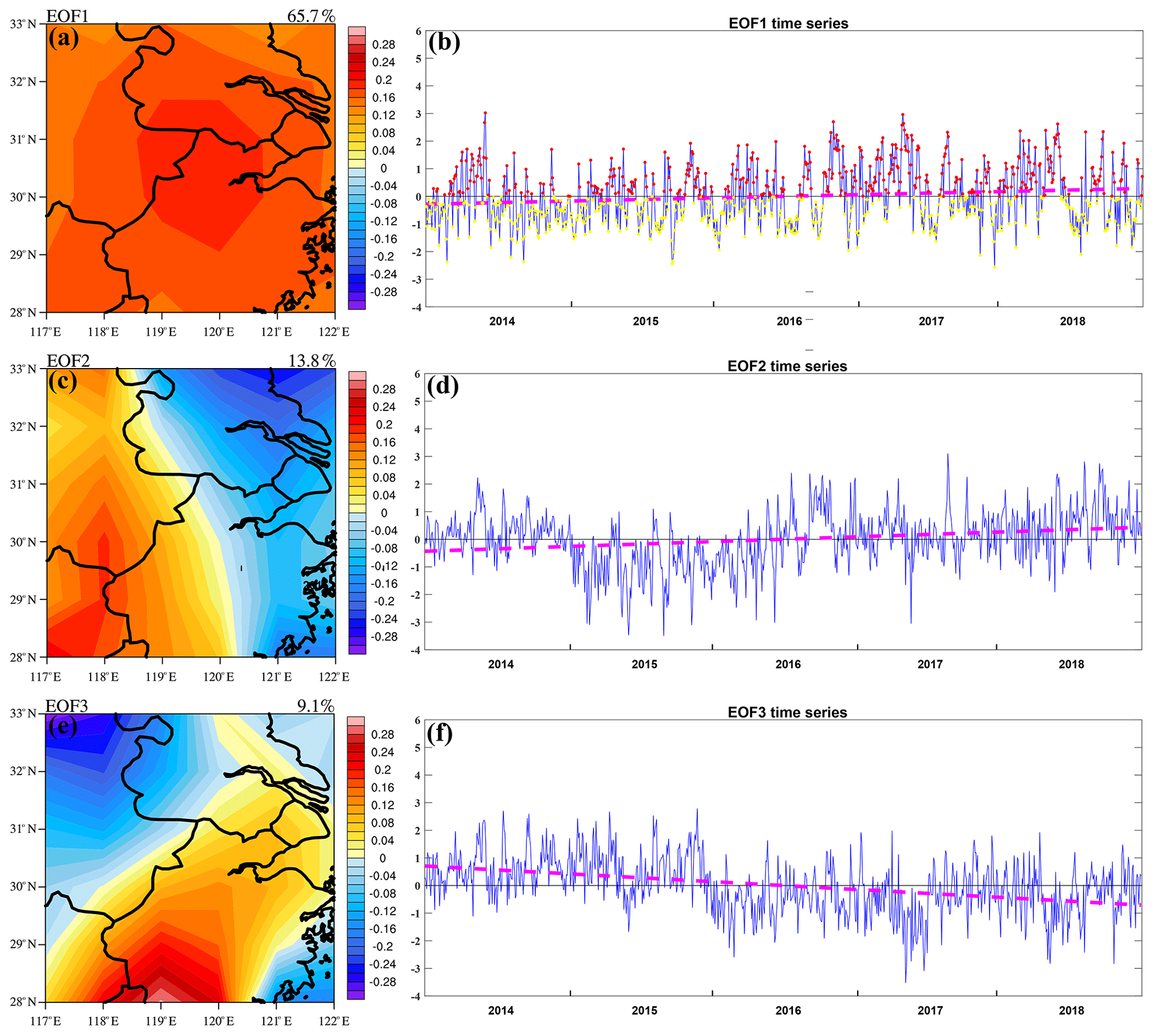
Figure 2Three EOF patterns of O3 concentration in the warm seasons from 2014 to 2018, including the spatial pattern (a, c, e) and time coefficient (b, d, f). The percentages in panels (a), (c) and (e) are the variance contributions of each EOF mode. The dashed pink line in panels (b), (d) and (f) represents the linear fitted curve.
3.2 Effects of meteorological conditions on O3 concentration over the YRD region
3.2.1 Quantifying the effects of meteorological conditions
With the primary pollutant emissions being cut down, the surface O3 increase in recent years in China might be attributable to a variety of factors, one of which was suggested to be the slowing down sink of hydroperoxy radicals, related to the variation in PM2.5 (Li et al., 2019). Yet, it is uncertain how meteorological conditions influence the increasing trend in surface O3. Yang et al. (2019) quantified the meteorological impact on O3 variation over the Pearl River Delta region using meteorological adjustment. Using a methodology similar to that in Yang et al. (2019), we investigate meteorological influences on the increase in ozone over the YRD in the warm seasons during 2014–2018. Figure 3a shows the ambient O3 variation from 2014 to 2018; i.e. O3 concentration increases from 2014, reaches a maximum in 2017 and maintains a relatively high level in 2018. After the meteorological adjustment, the variable magnitude is lower than the original one, implying that if the meteorological conditions remained unchanged over the 5 years, the variation in ambient O3 concentration would be lower. The meteorological impact can be examined from the difference between the solid and dashed black lines in Fig. 3a. The difference is negative from 2014 to the middle of 2016 and positive from the middle of 2016 to 2018. In 2017, the meteorological conditions increase O3 concentration by about 1.2 ppb. However, in 2015, the meteorological conditions become unfavorable to the O3 accumulation, leading to an O3 reduction of 1.4 ppb. The meteorological conditions make a difference in O3 concentration by 3.1 ppb at most between the most favorable year (2017) and the most unfavorable year (2015), which roughly corresponds to 8.7 % () of the annual O3 concentration.
In addition, we select the most influential meteorological factors to discuss their impacts on O3 variation, including T2, RH, SR, LCC and WS. As shown in Fig. 3b, RH is the most crucial factor, and its variation is similar to the variation in the total meteorological impact. In addition, SR and LCC also play important roles and have large impacts on O3 variation. RH can impact O3 concentration in two ways. One is gas-phase H2O reacting with O3 (). The other is its influence on clouds and thereby its shielding of SR. The East Asian summer monsoon plays a key role in affecting the local RH, and meanwhile it might bring a certain amount of O3 from the areas south of the YRD. However, O3 concentration is high negatively related to RH, which implies that local chemical reactions might contribute to the O3 accumulation more than the regional transport. The impacts of T2 and WS are inconsistent with the overall meteorological impacts.
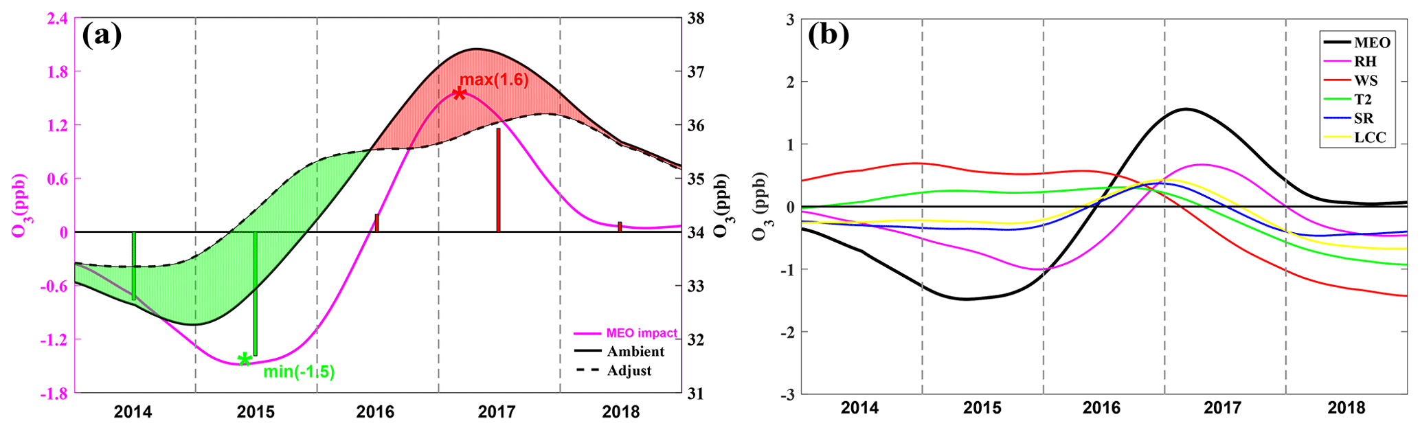
Figure 3(a) The 5-year trends of ambient O3 (solid black line), meteorological adjusted O3 (dashed black line) and the meteorological impact (pink line) over the YRD during 2014–2018. Periods with positive and negative meteorological impacts are shaded in red and green, respectively; red and green bars represent the O3 increases and decreases attributable to meteorological influences in each year. (b) The 5-year variations in the meteorological impact of different meteorological factors (MEO), including relative humidity (RH), solar radiation (SR), air temperature (T2), wind speed (WS) and low cloud cover (LCC).
3.3 Dynamic processes of O3 variation driven by synoptic circulations
As discussed in Sect. 3.2, the local meteorological factors have a large impact on the O3 variation. However, to some extent, the variation in local meteorological factors is largely affected by the synoptic-scale weather circulations (Leibensperger et al., 2008; Fiore et al., 2003; Wang et al., 2017). For example, in summer the YRD is under a hot, wet environment controlled by the WPSH, while in winter it is under a cold, dry environment, affected by the northwesterly flow caused by the Siberian High. The different weather systems under their corresponding SWPs have unique meteorological characteristics. Moreover, even under one SWP, the location and intensity changes in a specific weather system can cause changes in local meteorological factors correspondingly (Gao et al., 2020).
3.3.1 The main synoptic weather patterns in the warm season over the YRD
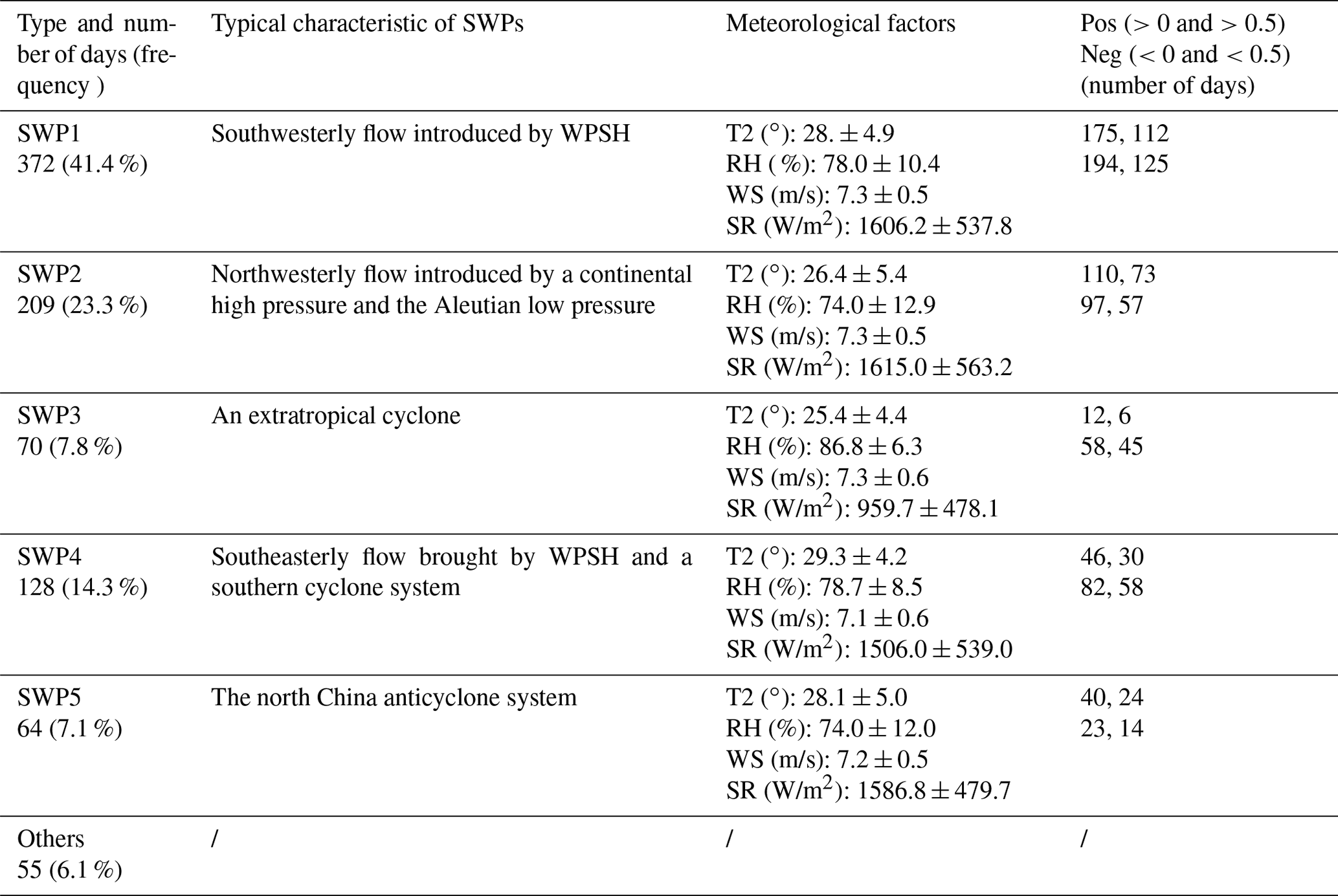
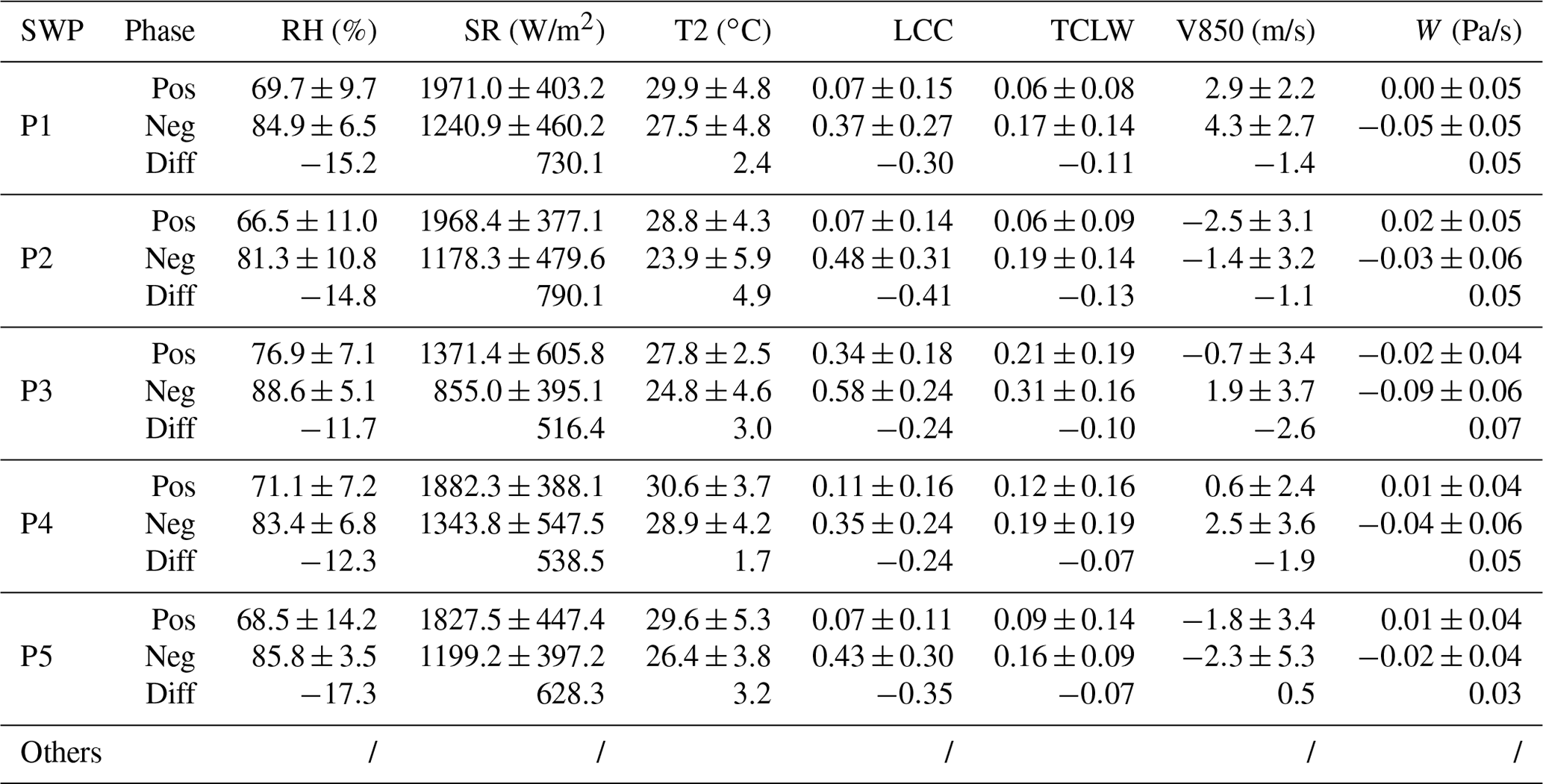
Applying the PTT classification method, nine SWPs are identified for the warm seasons in the YRD. Due to the relatively large variance, the first dominant five SWPs are selected, and the other four SWPs are grouped as “others”. As shown in Table 1, SWP1, SWP2 and SWP4 are dominant, accounting for 41.4 %, 23.3 % and 14.3 % of the occurrence frequency, respectively. In contrast, SWP3, SWP5 and other types occur in low frequencies, being 7.8 %, 7.1 % and 6.1 %, respectively. Specifically, SWP1 is under control of the southwesterly flow introduced by the WPSH. SWP2 is influenced by the northwesterly flow introduced by a continental high pressure and the Aleutian low pressure. SWP4 is influenced by the southeasterly flow introduced by the WPSH and a cyclone. SWP3 and SWP5 are affected by a cyclone and an anticyclone. SWP1 and SWP4 have high T2 and RH induced by the southerly flow, while under SWP5, the YRD has high T2 and low RH because the northerly flows are weakened and cannot carry sufficient water vapor. SWP2 has relatively low T2. SWP3 is under the control of a cyclone and the strong upward motion; it has weak SR and low T2. Specific figures of atmospheric circulation at 850 hPa under the five SWPs are provided in the Supplement.
Table 1The occurrence days and frequency, typical characteristics, regional mean ± the standard error for T2, RH, WS and SR and positive and negative days under each SWP. The >0 and >0.5 represent the value of EOF1 time series more than 0 and 0.5, respectively. The <0 and <0.5 show the opposite.
3.3.2 Impacts of SWP change on O3 concentration variation
We explore the impacts of SWP change on O3 variation through an analysis combined with EOF. As illustrated in Sect. 3.1.2, the EOF1 mode is the dominant mode, and it implies that an increase of O3 in the entire YRD region is the main trend. The EOF1 time series is closely correlated to the regional mean O3 concentration (R=0.98). In this study, we primarily focus on why O3 concentration increases in the entire YRD region, rather than on why the increases in O3 differ spatially inside the YRD. Therefore, we use the EOF1 time series as a proxy to present the regional O3 concentration. In Table 1, the positive phase (Pos) represents the EOF1 time series being more than 0, and it is beneficial to the production and accumulation of O3. Conversely, the negative phase (Neg) corresponds to low O3 concentrations. We extract the information by comparing Pos with Neg to find the changes in each SWP. Yin et al. (2019) explored dominant patterns of summer O3 pollution and associated atmospheric circulation changes in eastern China. Differently from their study, we analyzed the daily variation in SWPs and thus identified the change in atmospheric circulations more precisely.
In the five main SWPs, the EOF1 time series show an increase trend during their occurrence days in the warm seasons. It means that the five main SWPs tend to bring high ambient O3 concentration through changes in the SWPs, which include SWP changes in both frequency and intensity. We find that the change in SWP intensity impacts the inter-annual variation in O3 levels more significantly than the change in SWP frequency, consistent with the results of Hegarty et al. (2007) and Liu et al. (2019). This will be further discussed in Sect. 3.4. In the following, we will concretely discuss the variation characteristics of the five SWPs and their impacts on the increase of O3 in the YRD. In particular, we will show atmospheric circulations at 850 and 500 hPa, meteorological factors including SR, T2, LCC, TCLW, RH, meridional wind at 850 hPa (V850) and W (vertical velocity) under positive and negative phase of all SWPs and correlation coefficients of RH, SR and T2 with EOF1 time series under all SWPs.
As shown in a previous study, SR, T2 and RH are dominant meteorological factors and can directly impact O3 photochemical formation and loss (Xie et al., 2017; Gao et al., 2020). To explore the importance and difference of their impacts on O3 concentrations under different SWPs, we calculate the correlation coefficients between the EOF1 time series and these meteorological factors under each SWP. As shown in Tables 2 and 3, when the absolute values of the calculated correlation coefficients under a SWP are greater than 0.40, the corresponding meteorological factors present significant changes between Pos and Neg phases. Therefore, we regard them as the crucial meteorological factors that impact O3 variation under that SWP. In the end, we find that significant decreases in RH and increases in SR are the crucial meteorological factors under SWP1, SWP4 and SWP5. For SWP2, significant decreases in RH and increases in SR and T2 are the crucial meteorological factors. For SWP3, significant decreases in RH are the crucial meteorological factor. Hereinafter, we discuss variations in crucial meteorological factors induced by changes in atmospheric circulations.
Table 2Correlation coefficients of RH, SR and T2 with EOF1 time series under each SWP.

Figure 4 shows the atmospheric circulations at 850 and 500 hPa, and Table 3 shows meteorological factors including SR, T2, LCC, TCLW, RH, V850 and W for SWP1_Pos and SWP1_Neg. As shown in Fig. 4a and b, the YRD is located at the northwest of the WPSH, mainly affected by the southwesterly winds. Due to the weakening of the WPSH, compared with V850 of 4.3 m/s under SWP1_neg, weakening V850 of 2.9 m/s under SWP1_pos brings a lower amount of water vapor to the YRD region; therefore, RH significantly decreases by 15.2 %. At 500 hPa, a shallow trough located at approximate 113∘ E is replaced by a slow, straight westerly flow, and the downward motion would strengthen and last longer. In addition, significant decreases in RH under the downward motion condition hinder cloud formation. LCC and TCLW decrease by 0.30 and 0.11, respectively. Furthermore, SR significantly increases by 730.1 W/m2 due to less shelter of the clouds and less reflection above the clouds. Eventually, significant decreases in RH and increases in SR lead to a stronger O3 photochemical reaction.
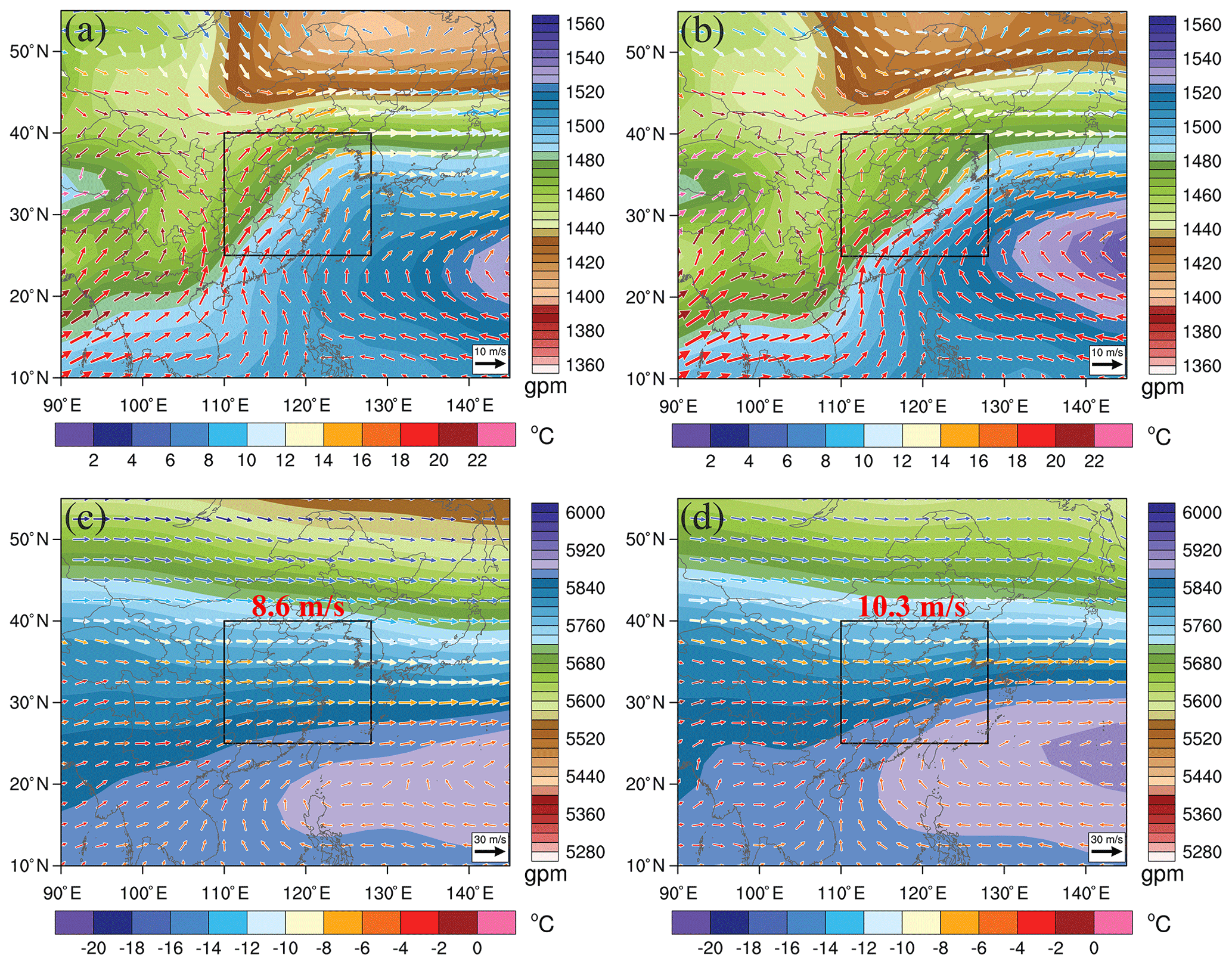
Figure 4The geopotential height (shaded) and 850 hPa wind with temperature (color vector) under (a) SWP1_Pos and (b) SWP1_Neg. The geopotential height (shaded) and 500 hPa wind with temperature (color vector) under (c) SWP1_Pos and (d) SWP1_Neg. The red values represent the regionally averaged wind speed at 500 hPa in the zone marked by black lines. The boxed area in panels (a)–(d) encloses the YRD.
Figure 5 shows the atmospheric circulations at 850 and 500 hPa, and Table 3 shows meteorological factors including SR, T2, LCC, TCLW, RH, V850 and W for SWP2_Pos and SWP2_Neg. As shown in Fig. 5a and b, the YRD is affected by a continental high and the Aleutian low, characterized by northwesterly flow and a slight southwesterly flow. Compared with the SWP2_Neg, the continental high in SWP2_Pos is weakening. Therefore, the YRD region is influenced by warm flows, and T2 significantly increases by 4.9 ∘C. The correlation between the EOF1 time series and T2 under SWP2 () is closer than the correlation in the whole period (). This implies that the weakening of the continental high plays an important role in enhancing O3 there. Meanwhile, as the Aleutian low moves southward slightly, the southwesterly flow can hardly bring water vapor to the YRD, which leads to significant decreases in RH by 14.8 %. At 500 hPa, a trough located at approximate 120–125∘ E is strengthened associated with the Aleutian low shifting southward, leading to a stronger downward motion in the northwestern YRD behind the strengthening trough. Just like SWP1, stronger downward motion and significantly decreasing RH enhance SR significantly by 790.1 W/m2. Significant decreases in RH and increases in SR and T2 are beneficial to O3 formation.
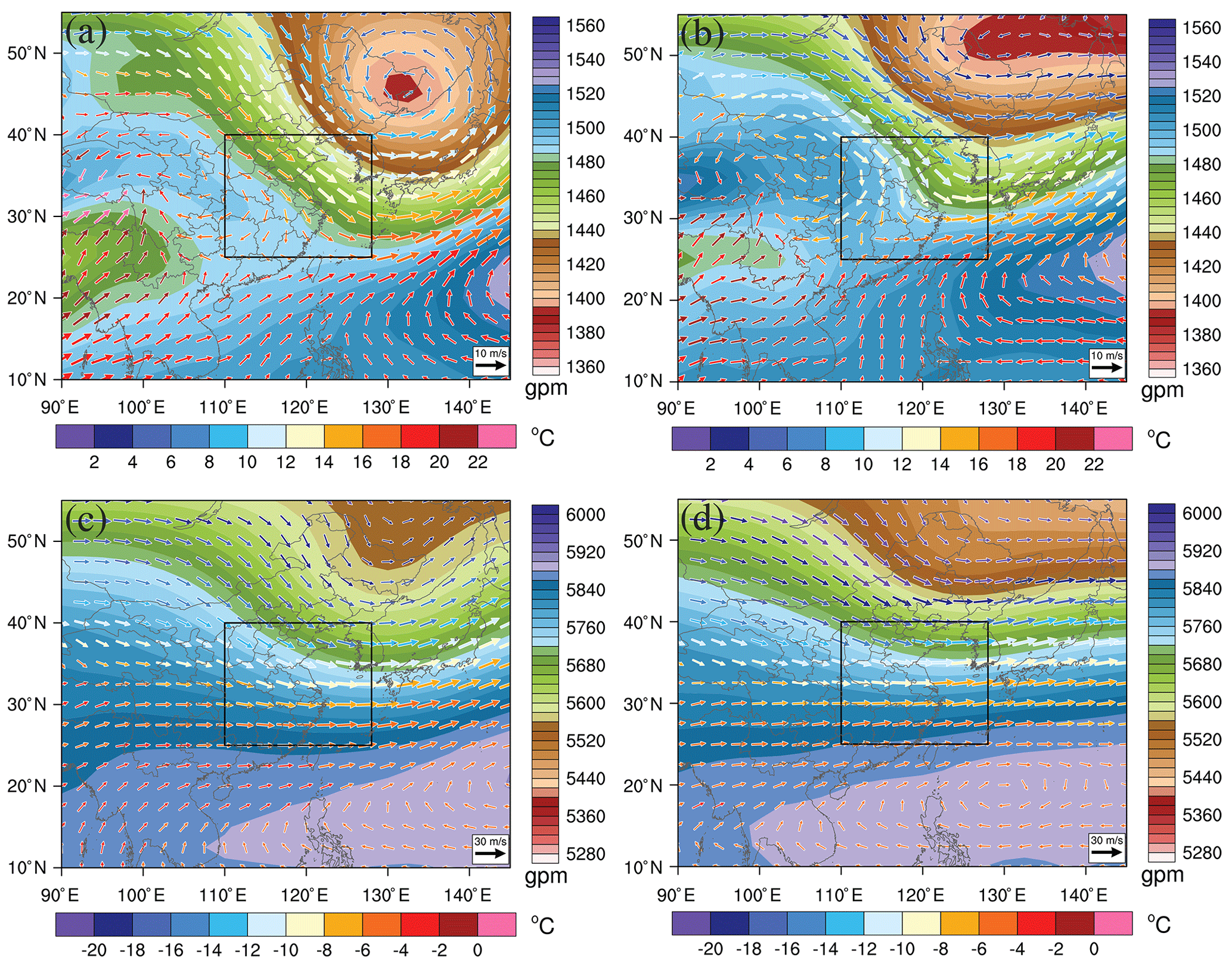
Figure 5The geopotential height (shaded) and 850 hPa wind with temperature (color vector) under (a) SWP2_Pos and (b) SWP2_Neg. The geopotential height (shaded) and 500 hPa wind with temperature (color vector) under (c) SWP2_Pos and (d) SWP2_Neg. The boxed area in panels (a)–(d) encloses the YRD.
Figure 6 shows the atmospheric circulations at 850 and 500 hPa, and Table 3 shows meteorological factors including SR, T2, LCC, TCLW, RH, V850 and W for SWP3_Pos and SWP3_Neg. As shown in Fig. 6a and b, the YRD is controlled by an extratropical cyclone. Compared with the SWP3_Neg, the low pressure in SWP3_Pos strengthens, and its location is slightly further eastward. Under this circumstance, the weakening southerly flow could hardly bring water vapor to the YRD, and thus RH significantly decreases by 11.7 %. At 500 hPa, the upward motion would be weakening due to the eastern movement of cyclone and western area controlled by back of a strengthening trough located at about 120∘ E. However, LCC still is at a high level under upward motion condition. Furthermore, high LCC and its lower variation lead to low SR. Therefore, the correlation coefficient between SR and EOF1 time series is relatively low under this SWP3 (). Lastly, only significant decreases in RH would be a crucial factor for high O3 concentration.
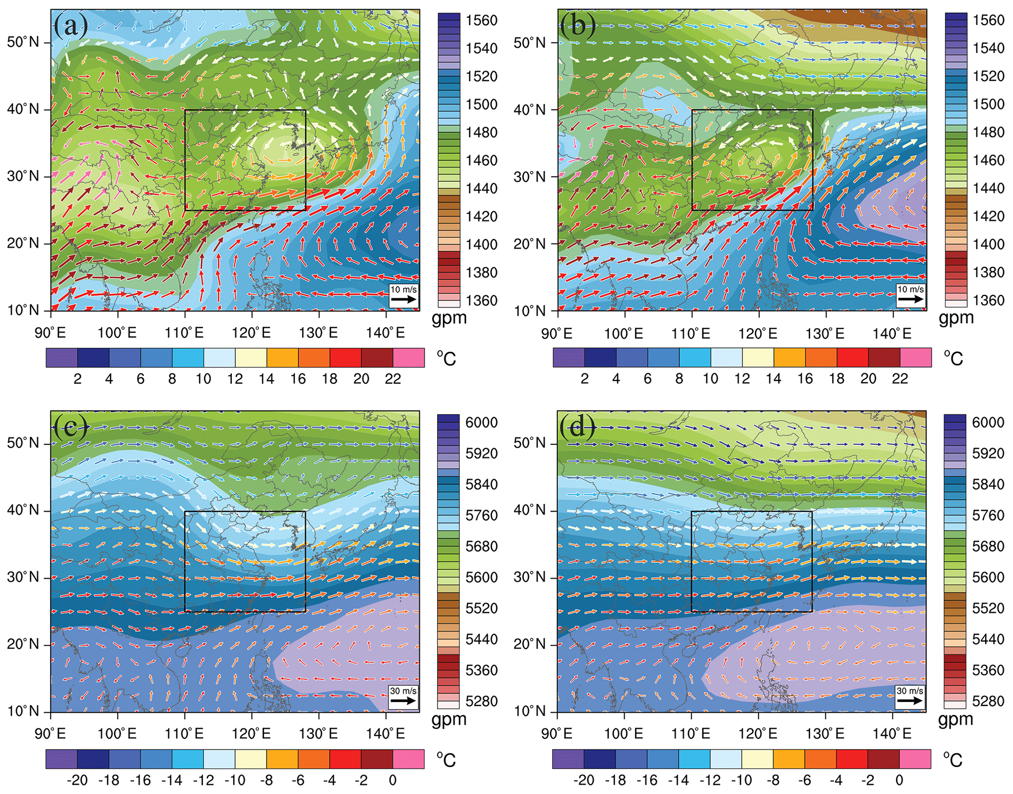
Figure 6The geopotential height (shaded) and 850 hPa wind with temperature (color vector) under (a) SWP3_Pos and (b) SWP3_Neg. The geopotential height (shaded) and 500 hPa wind with temperature (color vector) under (c) SWP3_Pos and (d) SWP3_Neg. The boxed area in panels (a)–(d) encloses the YRD.
Figure 7 shows the atmospheric circulations at 850 and 500 hPa, and Table 3 shows meteorological factors including SR, T2, LCC, TCLW, RH, V850 and W for SWP4_Pos and SWP4_Neg. As shown in Fig. 7a and b, southeasterly winds prevail in the YRD, which is modulated by a southern low pressure and WPSH. Compared with the SWP4_Neg, the southern low pressure and southeasterly flow in SWP4_Pos are weaker and thus bring less water vapor to the YRD and significantly decrease RH by 12.3 %. At 500 hPa, a shallow trough located at about 125∘ E strengthens, associated with weakening of the southern cyclone pressure, causing the strong sink motion, less LCC and significant increases in SR by 538.5 W/m2. Significant increases in SR and decreases in RH are important for O3 pollution.

Figure 7The geopotential height (shaded) and 850 hPa wind with temperature (color vector) under (a) SWP4_Pos and (b) SWP4_Neg. The geopotential height (shaded) and 500 hPa wind with temperature (color vector) under (c) SWP4_Pos and (d) SWP4_Neg. The boxed area in panels (a)–(d) encloses the YRD.
Figure 8 shows the atmospheric circulations at 850 and 500 hPa, and Table 3 shows meteorological factors including SR, T2, LCC, TCLW, RH, V850 and W for SWP5_Pos and SWP5_Neg. As shown in Fig. 8a and b, the YRD is controlled by the north China anticyclone, characterized by the northeasterly and the southwesterly winds. Compared with the SWP5_Neg, the high pressure in the SWP5_Pos is weaker, and the northeasterly flow responds accordingly. The weakened sea flow makes air drier and RH significantly lower by 17.3 %. At 500 hPa, a trough located at about 130∘ E controlling the YRD strengthens, associated with the appearance of low pressure over Japan. The downward motions become strong correspondingly and result in significant increases in SR by 628.3 W/m2. Significant increases in SR and decreases in RH lead to increases in O3 concentration.
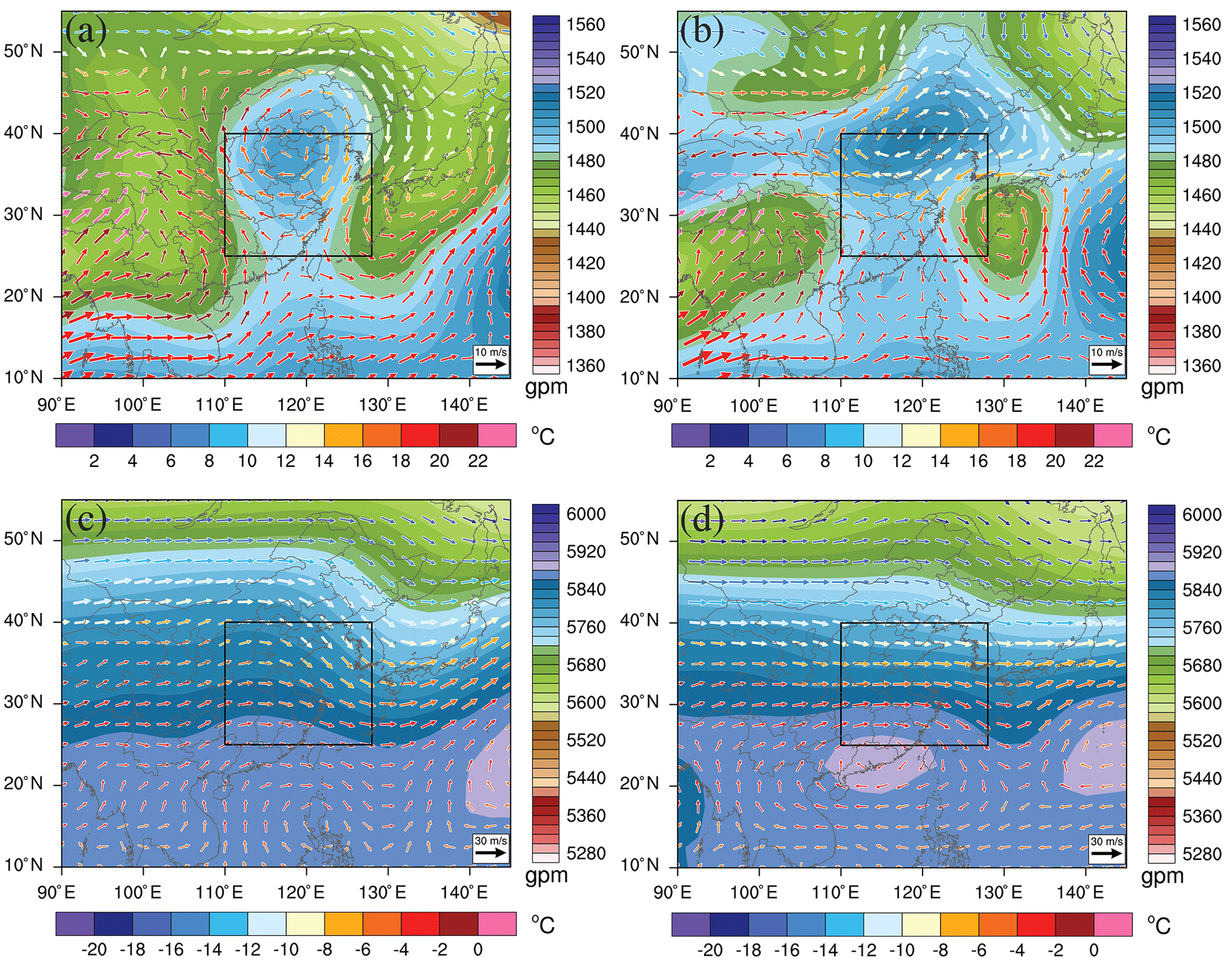
Figure 8The geopotential height (shaded) and 850 hPa wind with temperature (color vector) under (a) SWP5_Pos and (b) SWP5_Neg. The geopotential height (shaded) and 500 hPa wind with temperature (color vector) under (c) SWP5_Pos and (d) SWP5_Neg. The boxed area in panels (a)–(d) encloses the YRD.
Table 3Regional mean ± the standard error of meteorological factors in Pos and Neg phases and their difference (Diff) under each SWP pattern.
3.4 Indicators for reconstructing inter-annual O3 variation affected by synoptic-scale atmospheric circulation
Due to the similar variations in regional mean O3 concentration and EOF1 time series, we have reconstructed the inter-annual EOF1 time series to replace the regional mean O3 concentration by accounting for either frequency variation only or for both frequency and intensity variations in SWPs, which are EOF1 time series (Fre) and EOF1 time series (Fre + Int), respectively. The observed and reconstructed inter-annual EOF1 time series in 2014–2018 over the entire YRD region are shown in Fig. 9. Evidently, the frequency changes in SWPs almost have no impact on the O3 variability in the entire YRD region. However, considering intensity change, the fitting curve would be closer to the EOF1 time series. To obtain the accurate frequency and intensity change contributions, quantitative evaluation is carried out, and we define the contribution index as the difference between the maximum and the minimum of a certain reconstructed time series divided by the difference between the maximum and the minimum of the inter-annual EOF1 time series: contribution index = (the reconstructed maximum − the reconstructed minimum) (the original maximum − the original minimum). Through the above equation, we derive the relative contribution (contribution index) of the frequency change and the intensity change. Compared with the contribution index of 10.9 % for SWPs' frequency change, the value of 48.9 % for SWPs' intensity change accounts for a larger proportion. Therefore, the intensity change in SWP is more important for the inter-annual O3 variation than the frequency change.
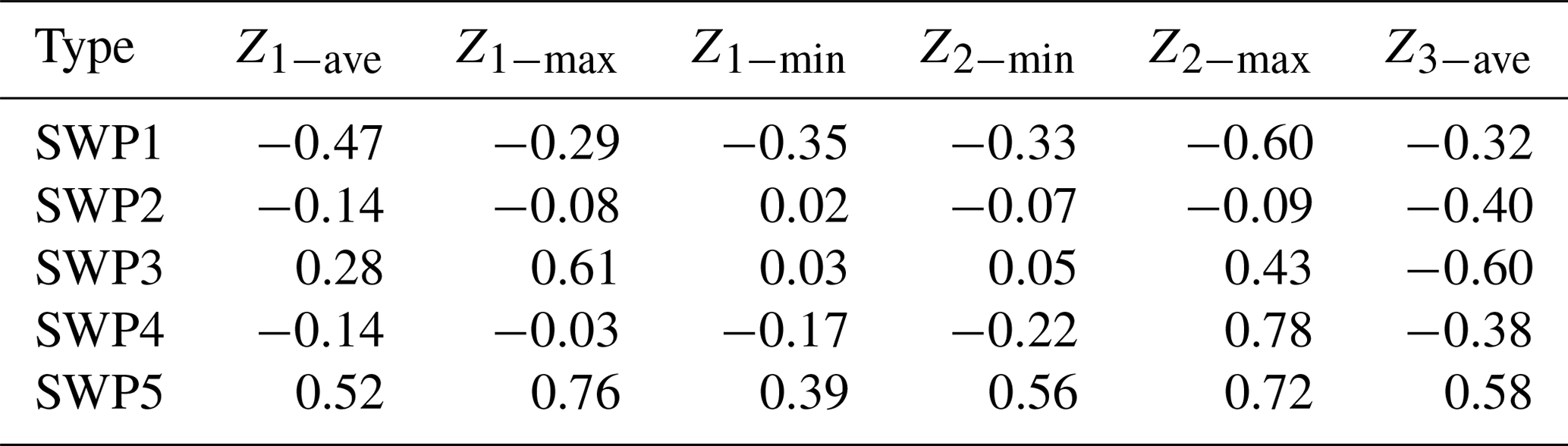
During the reconstruction process, we significantly found that the definition of the SWPIIs (SWP intensity indexes) plays an important role in reconstructing the curve. In previous studies, Hegarty et al. (2007) and Liu et al. (2019) reconstructed the inter-annual O3 level in the northeastern United States and northern China using the same method as ours. They defined the intensity change in SWPs using the domain-averaged sea level pressure and the pressure of the lowest-pressure system. However, the correlation under Hegarty's pattern V is poor, which has a negative effect on their reconstructed curve. Therefore, we select six SWPIIs and judge their rationality through their correlation coefficients with EOF1 time series under each SWP: the maximum geopotential height in zone 1 (25–40∘ N, 110–130∘ E) and zone 2 (20–50∘ N, 90–140∘ E), the minimum geopotential height in zone 1 (25–40∘ N, 110–130∘ E) and zone 2 (20–50∘ N, 90–140∘ E), and the average geopotential height in zone 1 (25–40∘ N, 110–130∘ E) and zone 3 (10–40∘ N, 110–130∘ E). As shown in Table 4, for SWP3 and SWP5, the SWPII for the maximum geopotential height in zone 1 has a relative high correlation. For SWP1 and SWP4, the SWPII for the maximum geopotential height in zone 2 has a relative high correlation. We found that the maximum geopotential height shows a relatively close correlation with the annual EOF1 time series. This is because the maximum geopotential height reflects the wind speed affecting water vapor transport under this pattern. Compared with SWP3 and SWP5, the weather systems are larger than the classification region for SWP1 and SWP4, so there are better correlation coefficients in zone 2 than in zone 1 under SWP1 and SWP4. For SWP2, when O3 concentration tends to be at a high level, a cold continental high behind the YRD tends to weaken. Therefore, we select the average geopotential height in zone 3 to represent the SWPII. Table 4 shows that the reconstructed curve improves when we select different SWPIIs according to the characteristics of a high O3 level under each SWP.
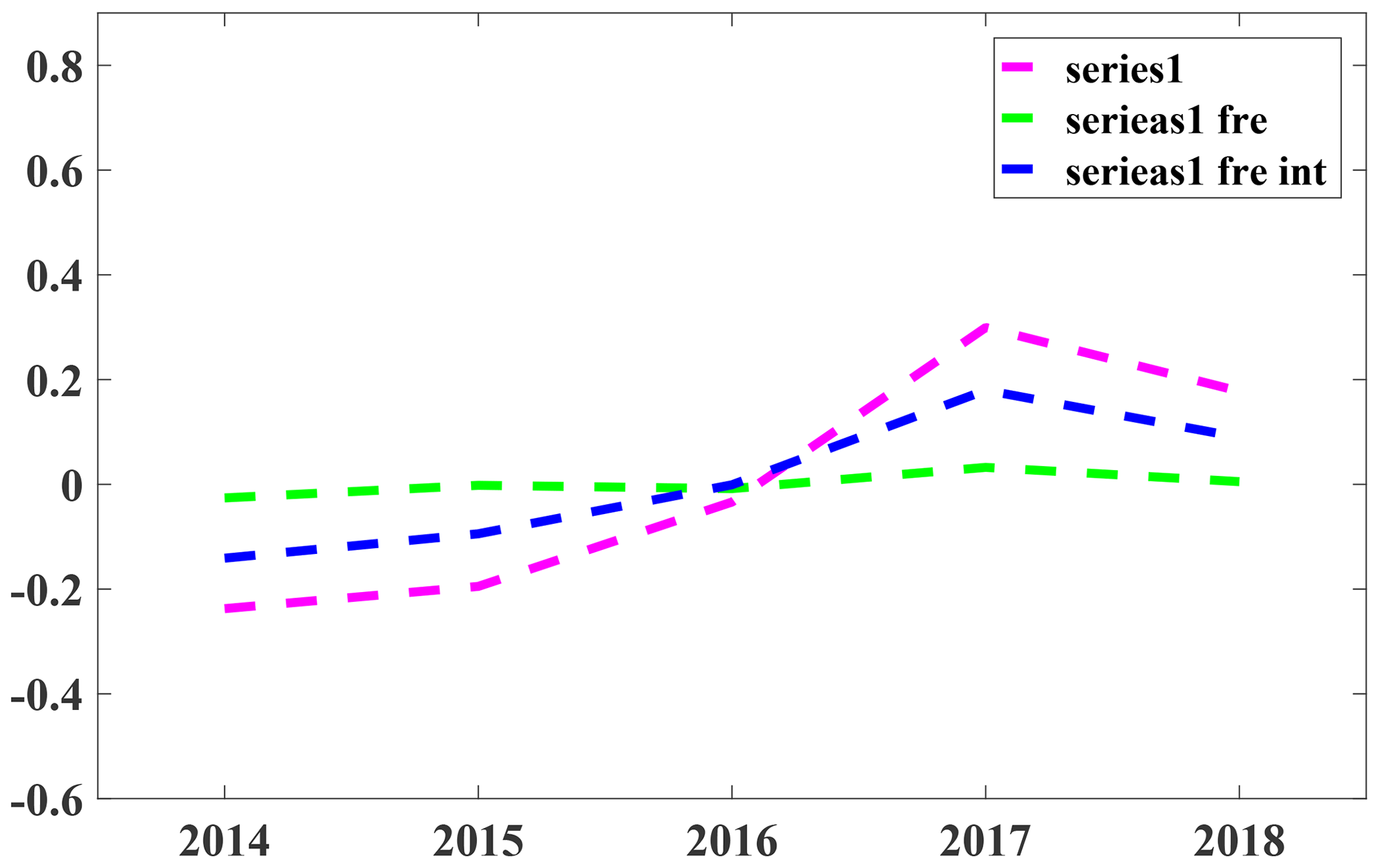
Figure 9The trend of the inter-annual EOF1 time series in the warm seasons. The pink curve represents the original inter-annual EOF1 time series in the warm seasons, the green line represents the reconstructed EOF1 time series only accounting for the frequency variation in SWPs and the blue line represents the reconstructed one, accounting for both the frequency and the intensity variations in SWPs.
Table 4Correlation coefficients between EOF1 time series and different SWPIIs under each SWP.
In this study, we discussed meteorological influences on the O3 variation in the warm seasons during 2014–2018 in the YRD, China. Specifically, we analyzed the O3 spatiotemporal distribution characteristics, quantified the contribution of meteorological conditions to the O3 variations, explored how changes in SWPs and corresponding meteorological factors lead to O3 increase in the YRD over 2014–2018 and assessed the contributions of SWP frequency and intensity to the inter-annual O3 variation in the region. The main conclusions are as follows.
The annual mean O3 concentrations during the warm seasons averaged over the YRD are 32.5, 33.0, 35.1, 37.4 and 36.0 ppb, respectively, for each year from 2014 to 2018, with a significantly increasing rate of 1.8 ppb/yr (5.2 %/yr). Meanwhile, the total number of days on which O3 concentration exceeding the national standard also increases each year in a similar pattern. Through the EOF analysis of O3 in space and time, three dominant modes were identified. The first mode is the most dominant mode, accounting for 65.7 % of the O3 variation, suggesting that increasing tendencies in O3 prevail over the entire YRD region.
We quantified the influence of meteorology on the inter-annual variation and trend of O3 over the YRD from 2014–2018 and found that the influence could lead to a regional O3 increase by 3.1 ppb at most. In particular, RH plays the most important role in modulating the inter-annual O3 variation, followed by SR and LCC. RH impacts O3 concentration in two ways. One is gas-phase H2O reacting with . The other is its influence on clouds and thereby its shielding of SR. To explore connections between the O3 variation and synoptic circulations, we further identified nine types of SWPs objectively based on the PTT method and selected five main types to explore their impact on O3 variation. The typical weather systems of the five SWPs include the WPSH under SWP1, a continental high and the Aleutian low under SWP2, an extratropical cyclone under SWP3, a southern low pressure and the WPSH under SWP4 and the north China anticyclone under SWP5. Combining EOF1 time series variation under each SWP, we found that the variation in all SWPs over 2014–2018 is favorable to O3 increase during that period. However, the crucial changes in meteorological factors attributable to the increases in O3 concentrations are different under each SWP. For SWP1, 4 and 5, the crucial changes in meteorological factors include significant decreases in RH and increases in SR, which are predominantly attributable to the WPSH weakening under SWP1, the southern low pressure weakening under SWP4, and the north China anticyclone weakening under SWP5. These changes in weather systems prevent the water vapor from being transported to the YRD and result in RH being significantly decreased by 15.2 %, 12.3 % and 17.3 %, respectively. Moreover, the significant decreases in RH and increases in downward motion (behind the strengthening trough and in front of the strengthening ridge) lead to less LCC, and thereby SR significantly increases by 730.1, 538.5 and 628.3 W/m2, respectively. Under SWP2, the crucial changes in meteorological factors are a significant decrease in RH by 14.8 % and increases in SR by 790.1 W/m2 and T2 by 4.9 ∘C. The significant decrease in RH and increases in SR are mainly induced by the Aleutian low extending southward, which has a similar influential mechanism between RH, LCC and SR with SWP1, 4 and 5. In addition, significant increases in T2 would be due to weakening cold flow introduced by a weakening continental high. Under SWP3, the significant decrease in RH by 11.7 % is mainly induced by an intensified extratropical cyclone that blocks the southerly flow carrying water vapor into the YRD. All changes are critical to O3 formation under each SWP.
As the overall change in SWP intensity and that in SWP frequency contribute to 48.9 % and 10.9 % to the changes in O3, we conclude that the change in SWP intensity is more important to the O3 increase over 2014–2018 than that in SWP frequency. We further reconstructed the EOF1 time series by considering different SWPIIs due to the unique characteristics of each SWP. The results are better than those in Hegarty et al. (2007) and Liu et al. (2019), who used the same SWPIIs in all SWPs.
This study quantified the inter-annual variation and increasing rate of O3 in the YRD, China, and explored the connection between SWP variations and the O3 increase. It provides an enhanced understanding of the response of O3 variation to changes in SWPs from year to year, and thus this understanding may be insightful in planning strategies for O3 pollution control.
The code used in this study is available upon request from Da Gao (dagao94@foxmail.com).
The maximum daily 8 h average O3 data were acquired from the air quality real-time publishing platform (http://106.37.208.233:20035, last access: 15 April 2021). Meteorological data were acquired from the National Meteorological Center of China Meteorological Administration (http://www.wmc-bj.net, last access: 15 April 2021) and the National Center for Environmental Prediction Final Operational Global Analysis (FNL) data (http://rda.ucar.edu/datasets/ds083.2/, last access: 15 April 2021).
The supplement related to this article is available online at: https://doi.org/10.5194/acp-21-5847-2021-supplement.
DG had the original ideas, collected and processed the data, designed the research study and prepared the original draft. MX helped DG to form the research ideas, discuss the results and revise the original draft and also provided financial support that led to this publication. JL and TW helped DG to collect the data and revise the paper. CM and HB helped DG to process the raw data. XC, ML, BZ and SL checked the English of the original paper.
The authors declare that they have no conflict of interest.
This research has been supported by the National Key Research and Development Program of China (grant nos. 2018YFC0213502 and 2018YFC1506404).
This paper was edited by Yugo Kanaya and reviewed by two anonymous referees.
Barnes, E. A. and Fiore, A. M.: Surface ozone variability and the jet position: Implications for projecting future air quality, Geophys. Res. Lett., 40, 2839–2844, https://doi.org/10.1002/grl.50411, 2013.
Cooper, O. R., Schultz, M. G., Schroder, S., Chang, K. L., Gaudel, A., Benitez, G. C., Cuevas, E., Frohlich, M., Galbally, I. E., Molloy, S., Kubistin, D., Lu, X., McClure-Begley, A., Nedelec, P., O'Brien, J., Oltmans, S. J., Petropavlovskikh, I., Ries, L., Senik, I., Sjoberg, K., Solberg, S., Spain, G. T., Spangl, W., Steinbacher, M., Tarasick, D., Thouret, V., and Xu, X. B.: Multi-decadal surface ozone trends at globally distributed remote locations, Elementa-Sci. Anthrop., 8, 23, https://doi.org/10.1525/Elementa.420, 2020.
Day, D. B., Xiang, J., and Mo, J.: Association of ozone exposure with cardiorespiratory pathophysiologic mechanisms in healthy adults, Jama Intern. Med., 177, 1400–1400, https://doi.org/10.1001/jamainternmed.2017.4605, 2017.
Doherty, R. M., Wild, O., Shindell, D. T., Zeng, G., MacKenzie, I. A., Collins, W. J., Fiore, A. M., Stevenson, D. S., Dentener, F. J., Schultz, M. G., Hess, P., Derwent, R. G., and Keating, T. J.: Impacts of climate change on surface ozone and intercontinental ozone pollution: A multi-model study, J. Geophys. Res.-Atmos., 118, 3744–3763, https://doi.org/10.1002/jgrd.50266, 2013.
Eskridge, R. E., Ku, J. Y., Rao, S. T., Porter, P. S., and Zurbenko, I. G.: Separating different scales of motion in time series of meteorological variables, B. Am. Meteorol. Soc., 78, 1473–1483, https://doi.org/10.1175/1520-0477(1997)078<1473:Sdsomi>2.0.Co;2, 1997.
Fiore, A. M., Jacob, D. J., Mathur, R., and Martin, R. V.: Application of empirical orthogonal functions to evaluate ozone simulations with regional and global models, J. Geophys. Res.-Atmos., 108, 4431, https://doi.org/10.1029/2002jd003151, 2003.
Gao, D., Xie, M., Chen, X., Wang, T. J., Liu, J., Xu, Q., Mu, X. Y., Chen, F., Li, S., Zhuang, B. L., Li, M. M., Zhao, M., and Ren, J. Y.: Systematic classification of circulation patterns and integrated analysis of their effects on different ozone pollution levels in the Yangtze River Delta Region, China, Atmos. Environ., 242, 117760, https://doi.org/10.1016/j.atmosenv.2020.117760, 2020.
Gao, W., Tie, X. X., Xu, J. M., Huang, R. J., Mao, X. Q., Zhou, G. Q., and Chang, L. Y.: Long-term trend of O3 in a mega City (Shanghai), China: Characteristics, causes, and interactions with precursors, Sci. Total Environ., 603, 425–433, https://doi.org/10.1016/j.scitotenv.2017.06.099, 2017.
Han, H., Liu, J., Shu, L., Wang, T., and Yuan, H.: Local and synoptic meteorological influences on daily variability in summertime surface ozone in eastern China, Atmos. Chem. Phys., 20, 203–222, https://doi.org/10.5194/acp-20-203-2020, 2020.
Hegarty, J., Mao, H., and Talbot, R.: Synoptic controls on summertime surface ozone in the northeastern United States, J. Geophys. Res.-Atmos., 112, D14306, https://doi.org/10.1029/2006jd008170, 2007.
Hou, X. W., Zhu, B., Kumar, K. R., and Lu, W.: Inter-annual variability in fine particulate matter pollution over China during 2013-2018: Role of meteorology, Atmos. Environ., 214, 116842, https://doi.org/10.1016/j.atmosenv.2019.116842, 2019.
Jacob, D. J. and Winner, D. A.: Effect of climate change on air quality, Atmos. Environ., 43, 51–63, https://doi.org/10.1016/j.atmosenv.2008.09.051, 2009.
Jerrett, M., Burnett, R. T., Pope, C. A., Ito, K., Thurston, G., Krewski, D., Shi, Y. L., Calle, E., and Thun, M.: Long-Term Ozone Exposure and Mortality., New Engl. J. Med., 360, 1085–1095, https://doi.org/10.1056/Nejmoa0803894, 2009.
Leibensperger, E. M., Mickley, L. J., and Jacob, D. J.: Sensitivity of US air quality to mid-latitude cyclone frequency and implications of 1980–2006 climate change, Atmos. Chem. Phys., 8, 7075–7086, https://doi.org/10.5194/acp-8-7075-2008, 2008.
Li, K., Jacob, D. J., Liao, H., Shen, L., Zhang, Q., and Bates, K. H.: Anthropogenic drivers of 2013–2017 trends in summer surface ozone in China, P. Natl. Acad. Sci. USA, 116, 422–427, 2019.
Liu, J., Wang, L., Li, M., Liao, Z., Sun, Y., Song, T., Gao, W., Wang, Y., Li, Y., Ji, D., Hu, B., Kerminen, V.-M., Wang, Y., and Kulmala, M.: Quantifying the impact of synoptic circulation patterns on ozone variability in northern China from April to October 2013–2017, Atmos. Chem. Phys., 19, 14477–14492, https://doi.org/10.5194/acp-19-14477-2019, 2019.
Lu, X., Hong, J. Y., Zhang, L., Cooper, O. R., Schultz, M. G., Xu, X. B., Wang, T., Gao, M., Zhao, Y. H., and Zhang, Y. H.: Severe Surface Ozone Pollution in China: A Global Perspective, Environ. Sci. Tech. Lett., 5, 487–494, https://doi.org/10.1021/acs.estlett.8b00366, 2018.
Lu, X., Zhang, L., Wang, X. L., Gao, M., Li, K., Zhang, Y. Z., Yue, X., and Zhang, Y. H.: Rapid Increases in Warm-Season Surface Ozone and Resulting Health Impact in China Since 2013, Environ. Sci. Tech. Lett., 7, 240–247, https://doi.org/10.1021/acs.estlett.0c00171, 2020.
Milanchus, M. L., Rao, S. T., and Zurbenko, I. G.: Evaluating the effectiveness of ozone management efforts in the presence of meteorological variability, J. Air Waste Manage., 48, 201–215, https://doi.org/10.1080/10473289.1998.10463673, 1998.
Papanastasiou, D. K., Melas, D., Bartzanas, T., and Kittas, C.: Estimation of Ozone Trend in Central Greece, Based on Meteorologically Adjusted Time Series, Environ. Model. Assess., 17, 353–361, https://doi.org/10.1007/s10666-011-9299-6, 2012.
Philipp, A., Beck, C., Huth, R., and Jacobeit, J.: Development and comparison of circulation type classifications using the COST 733 dataset and software, Int. J. Climatol., 36, 2673–2691, https://doi.org/10.1002/joc.3920, 2016.
Pu, X., Wang, T. J., Huang, X., Melas, D., Zanis, P., Papanastasiou, D. K., and Poupkou, A.: Enhanced surface ozone during the heat wave of 2013 in Yangtze River Delta region, China, Sci. Total Environ., 603, 807–816, https://doi.org/10.1016/j.scitotenv.2017.03.056, 2017.
Rao, S. T. and Zurbenko, I. G.: Detecting And Tracking Changes In Ozone Air-Quality, J. Air Waste Manage., 44, 1089–1092, https://doi.org/10.1080/10473289.1994.10467303, 1994.
Santurtun, A., Gonzalez-Hidalgo, J. C., Sanchez-Lorenzo, A., and Zarrabeitia, M. T.: Surface ozone concentration trends and its relationship with weather types in Spain (2001–2010), Atmos. Environ., 101, 10–22, https://doi.org/10.1016/j.atmosenv.2014.11.005, 2015.
Shu, L., Xie, M., Wang, T., Gao, D., Chen, P., Han, Y., Li, S., Zhuang, B., and Li, M.: Integrated studies of a regional ozone pollution synthetically affected by subtropical high and typhoon system in the Yangtze River Delta region, China, Atmos. Chem. Phys., 16, 15801–15819, https://doi.org/10.5194/acp-16-15801-2016, 2016.
Shu, L., Xie, M., Gao, D., Wang, T., Fang, D., Liu, Q., Huang, A., and Peng, L.: Regional severe particle pollution and its association with synoptic weather patterns in the Yangtze River Delta region, China, Atmos. Chem. Phys., 17, 12871–12891, https://doi.org/10.5194/acp-17-12871-2017, 2017.
Shu, L., Wang, T., Han, H., Xie, M., Chen, P., Li, M., and Wu, H.: Summertime ozone pollution in the Yangtze River Delta of eastern China during 2013–2017: Synoptic impacts and source apportionment, Environ. Pollut., 257, 113631, https://doi.org/10.1016/j.envpol.2019.113631, 2020.
Wang, B. and Fan, Z.: Choice of south Asian summer monsoon indices, B. Am. Meteorol. Soc., 80, 629–638, https://doi.org/10.1175/1520-0477(1999)080<0629:Cosasm>2.0.Co;2, 1999.
Wang, B., Wu, Z. W., Li, J. P., Liu, J., Chang, C. P., Ding, Y. H., and Wu, G. X.: How to measure the strength of the East Asian summer monsoon, J. Climate, 21, 4449–4463, https://doi.org/10.1175/2008JCLI2183.1, 2008.
Wang, T., Xue, L. K., Brimblecombe, P., Lam, Y. F., Li, L., and Zhang, L.: Ozone pollution in China: A review of concentrations, meteorological influences, chemical precursors, and effects, Sci. Total Environ., 575, 1582–1596, https://doi.org/10.1016/j.scitotenv.2016.10.081, 2017.
Wise, E. K. and Comrie, A. C.: Extending the Kolmogorov-Zurbenko filter: Application to ozone, particulate matter, and meteorological trends, J. Air Waste Manage., 55, 1208–1216, https://doi.org/10.1080/10473289.2005.10464718, 2005.
Xie, M., Zhu, K. G., Wang, T. J., Yang, H. M., Zhuang, B. L., Li, S., Li, M. G., Zhu, X. S., and Ouyang, Y.: Application of photochemical indicators to evaluate ozone nonlinear chemistry and pollution control countermeasure in China, Atmos. Environ., 99, 466–473, https://doi.org/10.1016/j.atmosenv.2014.10.013, 2014.
Xie, M., Liao, J., Wang, T., Zhu, K., Zhuang, B., Han, Y., Li, M., and Li, S.: Modeling of the anthropogenic heat flux and its effect on regional meteorology and air quality over the Yangtze River Delta region, China, Atmos. Chem. Phys., 16, 6071–6089, https://doi.org/10.5194/acp-16-6071-2016, 2016a.
Xie, M., Zhu, K., Wang, T., Chen, P., Han, Y., Li, S., Zhuang, B., and Shu, L.: Temporal characterization and regional contribution to O3 and NOx at an urban and a suburban site in Nanjing, China, Sci. Total Environ., 551–552, 533–545, https://doi.org/10.1016/j.scitotenv.2016.02.047, 2016b.
Xie, M., Shu, L., Wang, T.-j., Liu, Q., Gao, D., Li, S., Zhuang, B.-l., Han, Y., Li, M.-M., and Chen, P.-l.: Natural emissions under future climate condition and their effects on surface ozone in the Yangtze River Delta region, China, Atmos. Environ., 150, 162–180, https://doi.org/10.1016/j.atmosenv.2016.11.053, 2017.
Yang, L., Luo, H., Yuan, Z., Zheng, J., Huang, Z., Li, C., Lin, X., Louie, P. K. K., Chen, D., and Bian, Y.: Quantitative impacts of meteorology and precursor emission changes on the long-term trend of ambient ozone over the Pearl River Delta, China, and implications for ozone control strategy, Atmos. Chem. Phys., 19, 12901–12916, https://doi.org/10.5194/acp-19-12901-2019, 2019.
Yang, Y., Liao, H., and Li, J.: Impacts of the East Asian summer monsoon on interannual variations of summertime surface-layer ozone concentrations over China, Atmos. Chem. Phys., 14, 6867–6879, https://doi.org/10.5194/acp-14-6867-2014, 2014.
Yarnal, B.: Synoptic Climatology in Environmental Analysis A Primer, Journal of Preventive Medicine Information, 347, 170–180, 1993.
Yin, Z., Cao, B., and Wang, H.: Dominant patterns of summer ozone pollution in eastern China and associated atmospheric circulations, Atmos. Chem. Phys., 19, 13933–13943, https://doi.org/10.5194/acp-19-13933-2019, 2019.
Yue, X., Unger, N., Harper, K., Xia, X., Liao, H., Zhu, T., Xiao, J., Feng, Z., and Li, J.: Ozone and haze pollution weakens net primary productivity in China, Atmos. Chem. Phys., 17, 6073–6089, https://doi.org/10.5194/acp-17-6073-2017, 2017.
Zhang, J., Gao, Y., Luo, K., Leung, L. R., Zhang, Y., Wang, K., and Fan, J.: Impacts of compound extreme weather events on ozone in the present and future, Atmos. Chem. Phys., 18, 9861–9877, https://doi.org/10.5194/acp-18-9861-2018, 2018.
Zhao, Z. J. and Wang, Y. X.: Influence of the West Pacific subtropical high on surface ozone daily variability in summertime over eastern China, Atmos. Environ., 170, 197–204, 2017.