the Creative Commons Attribution 4.0 License.
the Creative Commons Attribution 4.0 License.
 | 01 Apr 2021
COVID-19 lockdown-induced changes in NO2 levels across India observed by multi-satellite and surface observations
Akash Biswal
Shweta Singh
Amit P. Kesarkar
Khaiwal Ravindra
Ranjeet S. Sokhi
Martyn P. Chipperfield
Sandip S. Dhomse
Richard J. Pope
Tanbir Singh
Suman Mor
We have estimated the spatial changes in NO2 levels over different regions of India during the COVID-19 lockdown (25 March–3 May 2020) using the satellite-based tropospheric column NO2 observed by the Ozone Monitoring Instrument (OMI) and the Tropospheric Monitoring Instrument (TROPOMI), as well as surface NO2 concentrations obtained from the Central Pollution Control Board (CPCB) monitoring network. A substantial reduction in NO2 levels was observed across India during the lockdown compared to the same period during previous business-as-usual years, except for some regions that were influenced by anomalous fires in 2020. The reduction (negative change) over the urban agglomerations was substantial (∼ 20 %–40 %) and directly proportional to the urban size and population density. Rural regions across India also experienced lower NO2 values by ∼ 15 %–25 %. Localised enhancements in NO2 associated with isolated emission increase scattered across India were also detected. Observed percentage changes in satellite and surface observations were consistent across most regions and cities, but the surface observations were subject to larger variability depending on their proximity to the local emission sources. Observations also indicate NO2 enhancements of up to ∼ 25 % during the lockdown associated with fire emissions over the north-east of India and some parts of the central regions. In addition, the cities located near the large fire emission sources show much smaller NO2 reduction than other urban areas as the decrease at the surface was masked by enhancement in NO2 due to the transport of the fire emissions.
- Article
(3916 KB) - Full-text XML
-
Supplement
(863 KB) - BibTeX
- EndNote


Nitrogen oxides, NOx (NO + NO2), are one of the major air pollutants, as defined by various national environmental agencies across the world, due to their adverse impact on human health (Mills et al., 2015). Furthermore, tropospheric levels of NOx can affect tropospheric ozone formation (Monks et al., 2015), contribute to secondary aerosol formation (Lane et al., 2008) and acid deposition, and impact climatic cycles (Lin et al., 2015). The major anthropogenic sources of NOx emissions include the combustion of fossil fuels in road transport, aviation, shipping, industries, and thermal power plants (e.g. USEPA and CATC, 1999; Ghude et al., 2013; Hilboll et al., 2017). Other sources include open biomass burning (OBB), mainly large-scale forest fires (e.g. Hilboll et al., 2017), lightning (e.g. Solomon et al., 2007), and emissions from soil (e.g. Ghude et al., 2010). NOx hotspots are often observed over regions with large thermal power plants and industries as well as urban areas with significant traffic volumes causing large localised emissions (e.g. Prasad et al., 2012; Hilboll et al., 2013; Ghude et al., 2013).
With growing scientific awareness of the adverse impacts of air pollution, the number of air quality monitoring stations has expanded to over 10 000 across the globe (Venter et al., 2020). Additionally, multiple satellite instruments such as the Global Ozone Monitoring Instrument (GOME) on ERS-2, the Scanning Imaging Absorption Spectrometer for Atmospheric Cartography (SCIAMACHY, 2002–2012) on Envisat, the Ozone Monitoring Instrument (OMI, 2005–present) on Aura, GOME-2 (2007–present) on MetOp, and the TROPOspheric Monitoring Instrument (TROPOMI, 2017–present) on Sentinel-5P (S5P) have monitored NO2 pollution from the space for over 2 decades. Surface sites typically measure NO2 in concentration quantities (e.g. in units of µg m−3), but satellite NO2 measurements are retrieved as integrated vertical columns (e.g. tropospheric vertical column density, VCDtrop). The latter is preferred for studying NO2 trends and variabilities because of global spatial coverage and spatio-temporal coincidence with ground-based measurements (Martin et al., 2006; Kramer et al., 2008; Lamsal et al., 2010; Ghude et al., 2011). NO2 has been reported to increase in south Asian countries (Duncan et al., 2016; Hilboll et al., 2017; ul-Haq et al., 2017) and decrease over Europe (van der A et al., 2008; Curier et al., 2014; Georgoulias et al., 2019) and the United States (Russell et al., 2012; Lamsal et al., 2015). In the case of India, a tropospheric NO2 increase was observed during the 2000s (e.g. Mahajan et al., 2015), but since 2012 it has either stabilised or even declined owing to the combined effect of economic slowdown and adoption of cleaner technology (e.g. Hilboll et al., 2017). However, thermal power plants, megacities, large urban areas, and industrial regions remain NO2 emission hotspots (Ghude et al., 2008, 2013; Prasad et al., 2012; Hilboll et al., 2013, 2017; Duncan et al., 2016). Moreover, despite the measures taken to control NOx emissions, urban areas often exceed national ambient air quality standards in India (Sharma et al., 2013; Nori-Sarma et al., 2020; Hama et al., 2020) and thus require a detailed scenario analysis.
The nationwide lockdown in various countries during March–May 2020, due to the outbreak of COVID-19, reduced traffic and industrial activities, leading to a significant reduction of NO2. Studies using space-based and surface observations of NO2 have reported reductions in the range of ∼ 30 %–60 % for China, South Korea, Malaysia, Western Europe, and the USA (Bauwens et al., 2020; Kanniah et al., 2020; Muhammad et al., 2020; Tobías et al., 2020; Dutheil et al., 2020; Liu et al., 2020; Huang and Sun, 2020; Naeger and Murphy, 2020; Barré et al., 2020; Goldberg et al., 2020) against the same period in previous years, with the observed reductions strongly linked to the restrictions imposed on vehicular movement. The lockdown in India was implemented in various phases starting on the 25 March 2020 (MHA, 2020; Singh et al., 2020). The lockdown restrictions in the first two phases (phase 1: 25 March–14 April 2020 and phase 2: 15 April–3 May 2020) were the strictest, during which all non-essential services and offices were closed, and the movement of the people was restricted, resulting in a considerable reduction in the anthropogenic emissions. The restrictions were relaxed in a phased manner from the third phase onwards in less affected areas by permitting activities and partial movement of people (MHA, 2020).
A decline in NO2 levels over India during the lockdown has been reported from both surface observations (Singh et al., 2020; Sharma et al., 2020; Mahato et al., 2020) and satellite observations (ESA, 2020; Biswal et al., 2020; Siddiqui et al., 2020; Pathakoti et al., 2020) against the previous year or average of a few previous years. A detailed study by Singh et al. (2020) based on 134 sites across India reported a decline of ∼ 30 %–70 % in NO2 during lockdown with respect to the mean of 2017–2019, with the largest reduction being observed during peak morning traffic hours and late evening hours. While Sharma et al. (2020) reported a smaller decrease (18 %) in NO2 for selected sites against the levels during 2017–2019, Mahato et al. (2020) found a decrease of over 50 % in Delhi for the first phase of lockdown against previous years (2017–2019), which was also confirmed by Singh et al. (2020) for the extended period of analysis. The satellite-based studies by Biswal et al. (2020) and Pathakoti et al. (2020) estimated the change in NO2 levels using OMI observations, whereas Siddiqui et al. (2020) used TROPOMI to compute the change over eight major urban centres of India. Biswal et al. (2020) reported that the average OMI NO2 over India decreased by 12.7 %, 13.7 %, 15.9 %, and 6.1 % during the subsequent weeks of the lockdown relative to similar periods in 2019. Similarly, Pathakoti et al. (2020) reported a decrease of 17 % in average OMI NO2 over India compared to the pre-lockdown period and a decrease of 18 % against the previous 5-year average. Moreover, both studies reported a larger reduction of more than 50 % over Delhi. Similarly, Siddiqui et al. (2020) also reported an average reduction of 46 % in the eight cities during the first lockdown phase with respect to the pre-lockdown phase. While recent studies have used either only satellite observations or only surface observations, this study goes further by adopting an integrated approach by combining both measurement types to investigate NO2 level changes over India in response to the COVID-19 pandemic using OMI, TROPOMI, and surface observations over different regions. As both OMI and TROPOMI have similar local overpass times of approximately 13:30 (Penn and Holloway, 2020; van Geffen et al., 2020), diurnal influences on the retrievals of NO2 for both instruments are similar. Moreover, as both instruments use nearly similar retrieval schemes (i.e. differential optical absorption spectroscopy, DOAS), their NO2 measurements are believed to be comparable with a suitable degree of confidence (van Geffen et al., 2020; Wang et al., 2020). Any product differences are likely to be caused by inconsistent inputs/processing of the retrievals (e.g. derivation of the stratospheric slant column, the a priori tropospheric NO2 profile, and the treatment of aerosols/clouds in the calculation of the air mass factor; van Geffen et al., 2019; Lamsal et al., 2021).
We estimate the changes in the NO2 levels over different land-use categories (i.e. urban, cropland, and forestland) and urban sizes. In addition to this, we investigate the spatial agreement between population density and NO2 spatial variability observed at the surface. A key benefit of this study will be to understand and assess the impact of reduced anthropogenic activity on NO2 levels, not only over the urban areas but also over the rural areas (cropland and forestland). This study thus provides an improved understanding of the spatial variations of tropospheric NO2 for future air quality management in India.
2.1 Data
Satellite observations of VCDtrop NO2 were obtained from OMI (2016–2020) and TROPOMI (2019–2020). Surface NO2 observations (2016–2020) at 139 sites across India were from the Central Pollution Control Board (CPCB). The period from 25 March to 3 May each year is defined as the analysis period. Average NO2 levels during the analysis period in 2020 and previous years are referred to as lockdown (LDN) NO2 and business-as-usual (BAU) NO2, respectively. The BAU years for OMI and CPCB are 2016–2019, whereas for TROPOMI the BAU year is 2019 because of the unavailability of earlier observations.
NO2 data were analysed for six geographical regions (north, Indo-Gangetic Plain (IGP), north-west, north-east, central, and south) of India (Fig. S1 in the Supplement). The NO2 changes over various land-use categories (i.e. urban, cropland, and forestland) have been analysed using spatially collocated land-use land cover (LULC) data (NRSC, 2012) and OMI- and TROPOMI-observed VCDtrop NO2. Visible Infrared Imaging Radiometer Suite (VIIRS) fire count data were used to study the fire anomalies during the LDN and other analysis periods.
2.1.1 OMI NO2
OMI has a nadir footprint of approximately 13 km × 24 km, measuring in the ultraviolet–visible (UV–Vis) spectral range of 270–500 nm (Boersma et al., 2011). It uses differential optical absorption spectroscopy (DOAS) to retrieve VCDtrop (i.e. VCDtrop is the difference between the total and stratospheric slant columns divided by the tropospheric air mass factor; Boersma et al., 2004). Here, we use the OMI NO2 30 % Cloud-Screened Tropospheric Column L3 Global Gridded (Version 4) at a 0.25∘ × 0.25∘ (∼25 km × 25 km) spatial grid from the NASA Goddard Earth Sciences Data and Information Services Center (GESDISC), available at (https://disc.gsfc.nasa.gov/datasets/OMNO2d_003/summary, last access: 1 January 2021). Details of the retrieval scheme and OMI data product Version 4 are discussed by Krotkov et al. (2019) and Lamsal et al. (2021) and for older versions by, for example, Celarier et al. (2008) and Krotkov et al. (2017).
2.1.2 TROPOMI NO2
TROPOMI has a nadir-viewing spectral range of 270–500 nm (UV–Vis), 675–775 nm (near-infrared, NIR), and 2305–2385 nm (shortwave-infrared, SWIR). In the UV-Vis and NIR wavelengths, TROPOMI has an unparalleled spatial footprint of 3.5 km × 7.0 km, along with 7 km × 7 km in the SWIR (Veefkind et al., 2012). Details of the TROPOMI scheme and data are discussed by Eskes et al. (2019) and Van Geffen et al. (2019). The TROPOMI VCDtrop NO2 over India for the analysis period was obtained at 3.5 km × 7 km resolution from http://www.temis.nl/airpollution/no2.php (last access: 25 December 2020) and re-gridded at a spatial resolution of 0.05∘ × 0.05∘ (∼5 km × 5 km) based on the gridding methodology of Pope et al. (2018). The source data are filtered to remove pixels with QA (quality assurance) values greater than 50, which removes cloud fraction less than 0.2, part of the scenes covered by snow/ice, errors, and problematic retrievals (Eskes et al., 2019).
Although substantial differences are found between OMI and TROPOMI (such as the differences in the orbit and spatial resolution; van Geffen et al., 2020), they exhibit good correlation with the surface observations (Chan et al., 2020; Wang et al., 2020) but are ∼30 % lower than the multi-axis differential optical absorption spectroscopy (MAX-DOAS) observations. Overall, TROPOMI has been reported to be superior to OMI (van Geffen et al., 2020). Detailed descriptions of the recent retrieval schemes used for TROPOMI and OMI data products are provided in van Geffen et al. (2019) and Lamsal et al. (2021), respectively. Analysis of differences between these two satellite data products is beyond the scope of this study.
2.1.3 Surface NO2 concentration
The hourly averaged surface NO2 concentration at 139 sites (Fig. S1) for 2016–2020 across India was acquired from the CPCB CAAQMS (Continuous Ambient Air Quality Monitoring Stations) portal (https://app.cpcbccr.com/ccr/#/caaqm-dashboard-all/caaqm-landing, last access: 1 December 2020). The data were further quality-controlled by removing the outliers, constant values, and sites with less than 60 % data during the analysis period. Details of the surface observations are explained in Singh et al. (2020).
2.1.4 Land use land cover data
The high-resolution (50 m × 50 m) LULC data mapped with level-III classification for 18 major categories (NRSC, 2012) were obtained from the Bhuvan geo-platform (https://bhuvan-app1.nrsc.gov.in/thematic/thematic/index.php, last access: 3 January 2020) of the Indian Space Research Organisation (ISRO). To quantify the changes over urban, crop, and forest areas, the OMI and TROPOMI NO2 at urban grids (category 1), cropland (category 2 to 5), and forestland (category 7 to 10) were extracted for further analysis. In order to match the OMI and TROPOMI grid resolution with the Indian LULC, the dominant LULC was considered within the OMI and TROPOMI grid. Figure S2 shows the high-resolution LULC data used in this study for cropland, forestland, and urban areas separately. Urban areas were further divided into four sizes (10–50, 50–100, 100–200, and greater than 200 km2) to study the change in NO2 with respect to the size of the urban agglomeration.
2.1.5 VIIRS fire counts
The VIIRS aboard the Suomi National Polar-orbiting Partnership (S-NPP) satellite provides daily global fire count at a 375 m × 375 m spatial resolution (Schroeder et al., 2014; Li et al., 2018). The fire count data over India during the analysis period from 2016 to 2020 were obtained from the FIRMS (Fire Information for Resource Management System) web portal (https://firms.modaps.eosdis.nasa.gov/download/, last access: 25 December 2020). The fire count data were gridded at 5 km × 5 km for each year by summing the fire counts falling on each spatially overlapping grid. The burnt area was calculated from the fire counts by multiplication by the VIIRS grid size (Prosperi et al., 2020).
2.1.6 Population data
The gridded population density (people per hectare, pph) data for 2020 were taken from Worldpop. (2017). Worldpop estimates the population density to be approximately 100 m × 100 m (near the Equator) by disaggregating census data for population mapping using a random forest estimation technique with remotely sensed and ancillary data. Details of the population mapping methodology can be found in Stevens et al. (2015).
2.1.7 Google mobility change
Google estimated the change in people's movement from 15 February 2020 onwards based on Google Maps information on people's locations at places of retail and recreation, grocery and pharmacy stores, parks, transit stations, workplaces, and residential places, etc. The changes were estimated with reference to the baseline days that represent a normal value for that day of the week. The baseline day is the median value from the 5-week period 3 January–6 February 2020. The Google mobility change dataset provided an excellent proxy for the anthropogenic activity change and has therefore been used for several purposes of air quality studies such as lockdown emission estimation and temporal relation with pollutant species (Archer et al., 2020; Forster et al., 2020; Gama et al., 2020; Guevara et al., 2021) during the lockdown period of 2020. The Google mobility data and reports are available from Google (2020).
2.1.8 Meteorological data
The Copernicus Climate Change Service (C3S) provides the ERA5 reanalysis (Hersbach et al., 2020) meteorological data with an improved vertical, temporal, and spatial coverage. The monthly mean meteorological data (temperature, wind speed, and planetary boundary layer height) at 0.25∘ × 0.25∘ resolution for March, April, and May 2016–2020 were used for the analysis. For details, see https://www.ecmwf.int/en/forecasts/datasets/reanalysis-datasets/era5 (last access: 25 January 2021).
2.1.9 Analysis methodology
The change in the NO2 levels for each analysis period has been calculated by subtracting the BAU NO2 from LDN NO2. We calculate the percentage change (D) using the following equation:
The analysis was done over the whole of India as well as over the separately considered regions and selected LULC categories using the open-source geographic information system QGIS.
3.1 Meteorological variations
Air pollutant concentration over a region is governed by emission sources and prevailing meteorological conditions. Meteorological factors (e.g. wind, temperature, radiation, and rainfall) can affect the NO2 concentration (Barré et al., 2020) as well as biogenic emissions (Guenther et al., 2012). The meteorological variations between years can cause ∼ 15 % variations in monthly column NO2 values (Goldberg et al., 2020). However, the NO2 levels are likely to be similar under similar meteorological conditions. Recent studies (e.g. Singh et al., 2020; Navinya et al., 2020; Sharma et al., 2020) have shown that meteorological conditions remained relatively consistent over recent years during the lockdown period and therefore assumed that the changes in the pollution levels during the lockdown are primarily driven by the emission changes. However, it is important to highlight the meteorological differences during the study period to assess the uncertainties associated with meteorological differences.
We used monthly mean ERA-5 reanalysis data (Hersbach et al., 2020) at 0.25∘ × 0.25∘ resolution for March, April, and May for BAU as well as LDN periods at the satellite local overpass time. We considered temperature (T), wind speed (WS), and boundary layer height (BLH) in our analysis. Figure 1a–c show the spatial variation in these quantities during BAU (left column), LDN (middle column) and the calculated difference (LDN−BAU, right column). The probability density function (PDF) using kernel density estimation (KDE) of the meteorological parameters is also shown (Fig. S3) for the BAU (blue) and LDN (red). KDE is a non-parametric way to estimate the PDF. The peak of the distribution shows the most probable value, and the width of the distribution shows the variability. The temperature difference between LDN and BAU shows a slight reduction (∼ 0–3 K range) during the lockdown. Wind speed values also show a reduction (up to 2 m s−1) during the lockdown, although the reduction is mainly seen in certain parts of central India. Reduction in the BLH is also seen in most parts of India. In general, the meteorological parameters during the lockdown were similar. However, the PDF (Fig. S3) during BAU and LDN shows a small reduction (less than 5 %) in temperature and wind speed and ∼ 10 % reduction in BLH. Although small, this weather variability can further add to the variability in the NO2 levels. However, during the lockdown in India, the NO2 change was more sensitive to the emission change than the meteorology variability. Shi et al. (2021) compared the detrended and de-weathered change in NO2 observed over selected cities in India, Europe, China, and the USA. While the reduction in NO2 was highest for Delhi (∼ 50 %), the difference between a detrended and de-weathered change in NO2 observed over Delhi was much smaller (∼ 2 %) as compared to the difference calculated for other cities. This suggests that weather variability did not have much impact on NO2 levels over India and that most of the changes were driven by a change in the anthropogenic emissions.

Figure 1Spatial map showing the variation in surface meteorological parameters (a temperature, b wind speed, and c BLH) from ERA-5 by comparing BAU (left column), LDN (middle column), and observed difference (LDN − BAU, right column).
3.2 Fire count anomalies during the lockdown
Forest fires are an important source of surface NO2 and VCDtrop NO2 (Sahu et al., 2015; Yarragunta et al., 2020), depending on the occurrence time and the intensity of fires (Mebust et al., 2011). Also, as the forest fire plumes can be transported longer distances (Alonso-Blanco et al., 2018), forest-fire-related NO2 can contribute to regional and global air pollution. In India, forest fires are prevalent as 36 % of the country's forest cover is prone to frequent fires, of which nearly 10 % is extremely to very highly prone to fires (ISFR, 2019). Long-term satellite-derived fire counts suggest that Indian fire activities typically peak during March–May (Sahu et al., 2015), predominantly over the north, central, and north-east regions (Venkataraman et al., 2006; Ghude et al., 2013). However, the spatial and temporal distribution of fire events is largely heterogeneous (Sahu et al., 2015), meaning an abrupt increase or decrease in fire activity could significantly impact NO2 levels over anomalous regions during the lockdown.
An investigation of fire counts during the 2020 lockdown (LDN analysis period), when compared with the corresponding 2016–2020 average, highlights a substantial decrease over the eastern part of central India and an increase over the western part of central India and the north-east. In Fig. 2a widespread fire activity (counts of 10–50) is shown across India, such as the central region (Madhya Pradesh, Chhattisgarh, Odisha), parts of Andhra Pradesh, the Western Ghats in Maharashtra, and the north-east region (Assam, Meghalaya, Tripura, Mizoram, and Manipur). The fire anomaly during the lockdown (Fig. 2b) shows positive fire counts (5–20) over the north-east region, west of Madhya Pradesh in central India, and scattered locations in South India. The negative fire anomalies (−20 to −5) observed over the central region (Chhattisgarh and Odisha) suggest a decrease in fire activity during the 2020 lockdown period. To minimise the impact of fire emission in our analysis, we have considered the grids with zero fire anomaly to assess the changes in NO2 during the lockdown. By considering the grids with zero fire anomaly, we excluded almost all the grids which have recorded fire activity during the analysis period. However, the impact of long-range transport of forest fire plumes cannot be ignored.

Figure 2Spatial distribution of the 5 km × 5 km gridded VIIRS fire counts. (a) Average fire counts during the analysis period (25 March–3 May 2016–2020). (b) Gridded fire anomaly during the lockdown in 2020.
3.3 VCDtrop NO2 over India during lockdown period
The spatial distribution of VCDtrop NO2 is largely determined by local emission sources; therefore, NO2 hotspots are found over urban regions, thermal power plants, and major industrial corridors. For the Indian subcontinent, maximum NO2 is observed during winter to pre-monsoon (December–May) and minimum NO2 during the monsoon (June–September). Region-specific peaks such as the wintertime peak (December–January) in the IGP are associated with anthropogenic emissions, or the summertime peak (March–April) in central India and north-east India is associated with enhanced biomass burning activities (Ghude et al., 2008, 2013; Hilboll et al., 2017).
We compare the LDN mean VCDtrop NO2 with the BAU mean for OMI and TROPOMI. The spatial distribution of the BAU and LDN VCDtrop NO2 observed by OMI and TROPOMI is shown in Fig. 3a–d. The mean VCDtrop NO2 from the two instruments shows similar spatial distributions during the LDN and BAU analysis period. In BAU years, the NO2 hotspots are seen over the large fossil-fuel-based thermal power plants (∼ 1000 × 1013 molec. cm−2), urban areas (∼ 400–700 × 1013 molec. cm−2), and industrial areas. Scattered sources are also present in western India, covering the industrial corridor of Gujarat and Mumbai, various locations of south India, and densely populated areas (e.g. IGP). The spatial distribution showed significant changes during the lockdown in 2020. The details of absolute and percentage changes are discussed in the subsequent sections.
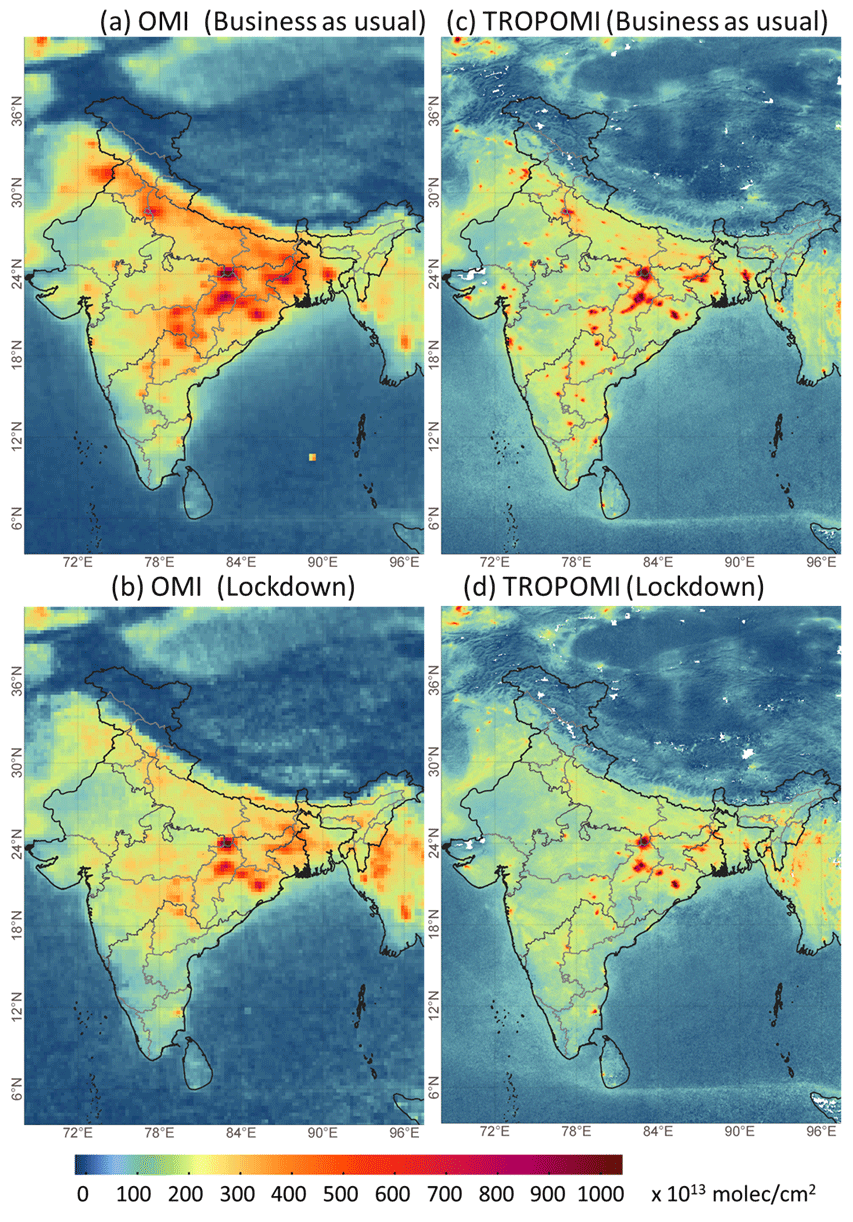
Figure 3Spatial distribution of mean VCDtrop NO2 (molec. cm−2) during the analysis period (25 March–3 May) for (a) OMI NO2 during business as usual (BAU, 2016–2019), (b) OMI NO2 during the lockdown (LDN, 2020), (c) TROPOMI NO2 during BAU (2019), and (d) TROPOMI NO2 during LDN (2020).
3.4 Changes observed by OMI and TROPOMI
There is a substantial reduction in VCDtrop NO2 between the LDN and BAU (Fig. 4a and c). A large reduction in the number of hotspots, mainly urban areas, is seen in both OMI and TROPOMI observations. However, hotspots due to coal-based power plants remain during the lockdown as electricity production was continued. Over the NO2 hotspots, there has been an absolute decrease of over 150 × 1013 molec. cm−2 (∼ 250 × 1013 molec. cm−2 over megacities) detected by both OMI and TROPOMI. The rural VCDtrop NO2 has typically reduced by approximately 30–100 × 1013 molec. cm−2, representing a percentage decrease of 30 %–50 % for OMI and 20 %–30 % for TROPOMI (Fig. 4b and d). For urban regions, both OMI and TROPOMI see a decrease of approximately 50 %, but reductions in smaller urban areas are clearly noticeable in the TROPOMI data, given its better spatial resolution. Both instruments observe an increase in VCDtrop NO2 in the north-eastern regions and moderate enhancement over the western and central regions. These enhancements are linked with the biomass burning activities during this period (Fig. 2).
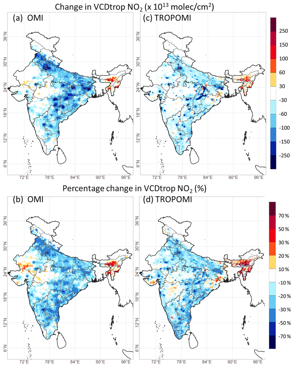
Figure 4(a, c) Absolute change and (b, d) percentage change in VCDtrop NO2 during the analysis period for LDN year compared to BAU years as observed by OMI (a, b) and TROPOMI (c, d).
3.5 Changes in NO2 over different land use types
Anthropogenic NOx emissions are typically more localised in urban and industrial centres, while biogenic sources (e.g. soil) are more important in rural regions. OBB activities peak in March–April (Sahu et al., 2015) and represent more sporadic sources. As the lockdown is expected to have reduced urban anthropogenic NOx sources (as shown in Fig. 4), it is important to assess the lockdown impact over the rural regions such as cropland and forestland as well. This section estimates the changes in VCDtrop NO2 over different land types such as cropland, forestland, and urban areas (Fig. S2). Industrial emissions are often part of the urban agglomerates scattered around the city and are part of urban emissions. To minimise the impact of OBB emissions in our analysis, we exclude grids with fire anomalies (Fig. 2) and those containing thermal power plants (Fig. S2d). However, absolute separation of the impact of long-range transportation is beyond the scope of this study.
3.5.1 Changes over cropland and forestland
The changes in VCDtrop NO2 observed by OMI and TROPOMI over the cropland (Fig. S2a) in different regions of India are shown in Fig. 5a and b and Table S1 in the Supplement. A decline in VCDtrop NO2 has been observed over croplands in all regions except for the north-east. A higher percentage decline was observed over IGP and south regions by both the satellites. While VCDtrop NO2 has decreased, prominent enhancements have been observed over the north-east and few grids in central and north-west regions. These enhancements can be attributed to the impact of nearby forest fires (Fig. 2). The observed changes over the forestland (Fig. S2c) over different regions of India are shown in Fig. 5c–d and Table S1. The average VCDtrop NO2 has declined over forestland in all the regions except for the north-east, where VCDtrop NO2 was enhanced due to the positive fire anomaly (Fig. 2) during the analysis period. It can be noted that although we have taken the grids with zero fire anomaly, the effect of a nearby grid exhibiting positive fire anomaly cannot be ignored due to atmospheric dispersion and mixing. The inter-comparison of the changes observed by two satellites suggests that OMI data indicate a larger reduction in VCDtrop NO2 than TROPOMI in most of the regions.
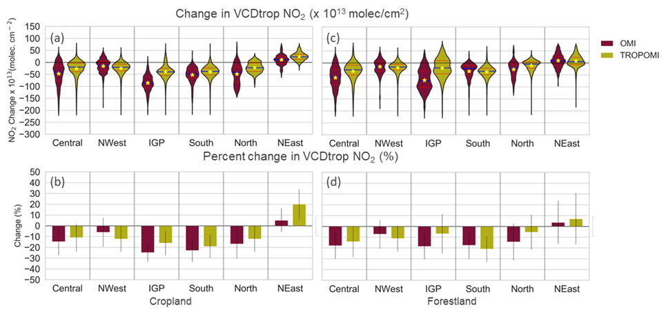
Figure 5Observed change in VCDtrop NO2 between LDN and BAU from OMI and TROPOMI for different regions shown as (a) a violin plot of the absolute change over cropland, (b) the percentage change over cropland, (c) a violin plot of the absolute change over forestland, and (d) the percentage change over forestland. A violin plot is a combination of a box plot and a kernel density estimation (KDE) plot. KDE is a non-parametric way to estimate the probability density function (PDF). The red lines in the violin plot show the interquartile range; the blue line shows the median value; the yellow star shows the mean value. The vertical lines in the bar plot show the standard deviation. The abbreviations NWest and NEast are for north-west and north-east regions, respectively.
3.5.2 Changes over urban regions
We analysed the changes in VCDtrop NO2 over the urban areas (Fig. S2b) in different regions of India. The calculated actual and percentage changes observed by OMI and TROPOMI are shown in Fig. 6 and in Table S1. The mean changes observed by OMI and TROPOMI show similar variations in different regions. The changes observed over urban areas are larger than those observed over the forest and croplands. In contrast to the cropland and forestland, TROPOMI observed a larger reduction in VCDtrop NO2 than OMI in most of the regions. Densely populated IGP with the largest urban agglomeration shows the maximum change in VCDtrop NO2 followed by the central and north-west regions. The VCDtrop NO2 over the urban areas in the north-east region is likely to be influenced by the nearby forest fires through atmospheric dispersion and mixing, resulting in the enhancement of VCDtrop NO2 over the urban grids.
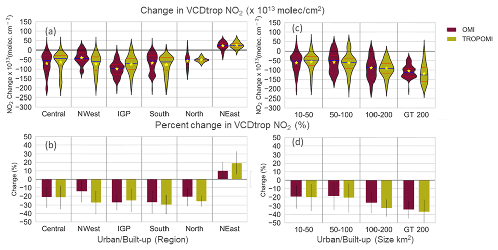
Figure 6Observed change in VCDtrop NO2 between LDN and BAU from OMI and TROPOMI for different regions shown as (a) a violin plot of the absolute change over urban areas, (b) the percentage change over the urban area, (c) a violin plot of the observed change over different sized urban areas, and (d) the percentage change over different sized urban areas.
We have also analysed the change in the VCDtrop NO2 over urban areas of different sizes. We have taken the urban areas of sizes more than 10 km2 and grouped them into four bins of size 10–50, 50–100, 100–200, and greater than 200 km2. We then calculate the changes observed for all the cities filling into the respective bins. Figure 6c–d show the absolute and percentage change in VCDtrop NO2, as observed by OMI and TROPOMI, respectively. A significant reduction of 50–150 × 1013 molec. cm−2 (20–40 %) was observed over the urban area of different sizes. The actual reduction in VCDtrop NO2 is greater for the larger urban area, with peak reductions for the urban area bin (>200 km2) for both OMI and TROPOMI. The greater reduction in the larger urban areas is mainly due to the reduction in local emission sources, as evidenced by the Google mobility reduction, which is higher for larger cities than the smaller ones (Fig. S6).
3.5.3 Changes over thermal power plants
Thermal power plants (TPPs) are the hotspots of NO2 pollution. These are scattered across the nation, with the majority of them in Madhya Pradesh, Bihar, Uttar Pradesh, Odisha, Gujarat, Chhattisgarh, West Bengal, and Tamil Nadu (Fig. S2d). During the lockdown period, TPPs were still operated to fulfil electricity demands. In this section, we analyse the changes observed over TPPs. The changes in VCDtrop NO2 observed by OMI and TROPOMI over the TPPs are shown in Fig. S5. A decrease in mean VCDtrop NO2 levels over TPPs has been observed that is in line with the power sector report, which mentions that during April 2020, energy demand met for India decreased by 24 % as compared to April 2019 (POSOCO, 2021). Also, there is a drop (∼ 30 %) in thermal power production during the lockdown compared to the respective period of 2019.
3.6 Inter-comparison of changes observed by OMI, TROPOMI and surface observation
Figure 7a–b show the relationship of OMI and TROPOMI NO2 with surface NO2 for the BAU and LDN periods, respectively. During BAU, there are reasonable positive correlations between the satellite instruments and the surface sites (OMI: 0.48, 95 % CI 0.33–0.60 and TROPOMI: 0.52, 95 % CI 0.37–0.64). In LDN, these correlations drop to 0.36 (95 % CI 0.20–0.49) and 0.28 (95 % CI 0.12–0.43), respectively. The decrease in the correlation during LDN could be due to the decrease in the signal-to-noise ratio, potentially linked with the primary reduction in urban NO2 levels. We also determined the correlation between satellite- and surface-observed changes during the lockdown (Fig. 7c), finding values of 0.44 (95 % CI 0.28–0.57) for OMI and 0.49 (95 % CI 0.33–0.63) for TROPOMI. This indicates that the lockdown NO2 reductions appear to be present in both measurement types, providing us with confidence in the observed changes detected in this study. The correlation observed over India in this study is lower than that reported for the USA (Lamsal et al., 2015). The low correlation between OMI and surface NO2 has been reported previously by Ghude et al. (2011). While they report the temporal correlation for a single site, our study reports the spatial correlation representing the satellites' ability to capture the spatial heterogeneity. One of the reasons for the lower correlation could be the choice of surface station. Generally, urban background sites are preferred for this kind of analysis. However, the surface NO2 monitoring station type classification is not available for the CPCB sites. Therefore, sites used in the analysis could be potentially impacted by traffic emissions, resulting in lower correlation. Another reason is that in situ measurements are more sensitive to the local emission sources than remotely sensed measurements and therefore have larger variability, resulting in low correlation. Proper classification of the monitoring stations could provide a better assessment of satellite-based observations.

Figure 7Scatter plots between surface- and satellite-observed NO2 for (a) business as usual (BAU) and (b) lockdown (LDN). Panel (c) shows a scatter plot of observed absolute change (LDN − BAU) in surface and satellite NO2. The values shown in the brackets are the correlation coefficients with 95 % confidence intervals (CIs).
The LDN NO2 percentage change, observed by surface and spatially co-located satellite measurements, is shown in Fig. 8a for various Indian regions. For this comparison, the number of available CPCB surface monitoring stations was 17, 15, 81, 25, and 1 for central, north-west, IGP, south, and north-east regions (north region data not available), respectively. Most of the CPCB stations are in urban areas, so our results reflect changes in predominantly urban-sourced NO2. At all surface sites in all regions, there was a percentage reduction greater than 20 % (Fig. 8a). Satellite observations show a similar trend except for the north-east region, where enhancements are due to forest fires. Both OMI and TROPOMI observed the highest reduction (∼ 50 %) over IGP. A smaller average reduction of ∼ 20 % over central India might be due to the aggregate effect of power plants, forest fires, and prevalent biomass burning activities during this season. While the effect of forest fires can be observed in the column NO2, its impact on the surface NO2 is minimal. For the central, IGP, and south regions, the mean percentage change observed by the surface monitoring station is comparable to that observed by the satellites.

Figure 8(a) Box plot showing the percentage change between LDN and BAU in NO2 levels observed by ground and satellite measurements at CPCB monitoring locations in different regions. (b) Bar chart showing the percentage change in NO2 levels observed in megacities in India for the same measurements as panel (a). The vertical line in the bar chart is the standard deviation.
We have inter-compared the percentage change in NO2 observed at the surface and satellite over the major Indian cities (i.e. New Delhi, Chennai, Mumbai, Bangalore, Ahmedabad, Kolkata, and Hyderabad; Fig. 8b). A significant reduction in the range of ∼ 25 %–75 % is observed, consistent in all observational sources used in this study. A similar reduction observed by the satellites over the cities in other parts of the world has been reported (Tobías et al., 2020; Naeger and Murphy, 2020; Kanniah et al., 2020; Huang and Sun, 2020). The satellites observe the largest reduction over Delhi and the smallest over Kolkata. While the observed decline is comparable for cities, Ahmedabad and Kolkata showed smaller declines than observed by ground measurements. Also, the reduction observed at the surface has a larger spatial variability than the one observed from the space. This is potentially linked to the influence of the local emissions which could not be detected by the space-based instruments because of relatively large satellite footprints. The results of percentage change observed by OMI are consistent with the change reported by Pathakoti et al. (2020), although Siddiqui et al. (2020) reported a higher decline of NO2 using TROPOMI. This is because we computed the changes between lockdown and BAU during the same period of the year, whereas Siddiqui et al. (2020) estimated the changes between the pre-lockdown NO2 and the lockdown NO2, which includes the seasonal component of NO2. We have also analysed the changes in VCDtrop NO2 observed by both OMI and TROPOMI for the other major cities (Guttikunda et al., 2019), as shown in Fig. S4. A reduction of over 20 % was observed in most cities except for a few in north-east and central India. Cities showing enhancement or smaller reductions reflect the enhanced fire activities in the north-east and central Indian regions. TROPOMI can capture the reduction over the cities near the fire-prone areas (e.g. Indore and Bhopal) because of its higher spatial resolution.
3.7 Correlation of tropospheric columnar NO2 with the population density
In this section, we examine the VCDtrop NO2 and population relationship for India except where fire anomalies or large thermal power plants existed. The scatter density plots between VCDtrop NO2 and population density for the BAU and LDN analysis period are shown in Fig. 9 for OMI and TROPOMI. The data were log-transformed to establish the log–log relationship as neither dataset is normally distributed. As the observed changes had negative values, this log transformation was obtained by adding a constant value (Ekwaru and Veugelers, 2018), which was later subtracted when plotting to display the corresponding NO2 values. Both OMI and TROPOMI NO2 show a similar relationship with the population density, with correlations of ∼ 0.65 during the LDN and BAU periods, suggesting a strong dependence upon the population (i.e. anthropogenic emissions). The slopes of the lines in Fig. 9a, b, d, and e show that VCDtrop NO2 follows a power-law scaling with population density (Lamsal et al., 2013). During BAU, the VCDtrop NO2 observed over a grid increased by factors of 100.28=1.9 and 100.20=1.58 for OMI and TROPOMI, respectively, with a 10-fold increase in the population density. The rate of increase of the VCDtrop NO2 during LDN was 100.23=1.7 and 100.16=1.45 times for OMI and TROPOMI, respectively, which was lower than BAU. The correlation during the LDN period was marginally lower than the BAU period. This could be due to a larger reduction in the NO2 levels in the densely populated grids. The changes observed in the VCDtrop NO2 during the LDN (Fig. 9c and f) were negatively correlated (i.e. reduction was positively correlated) with the population density. The linear relation suggests an increase in the reduction with an increase in the population density; however, some grids exhibit enhancements in VCDtrop NO2 due to the local emissions.
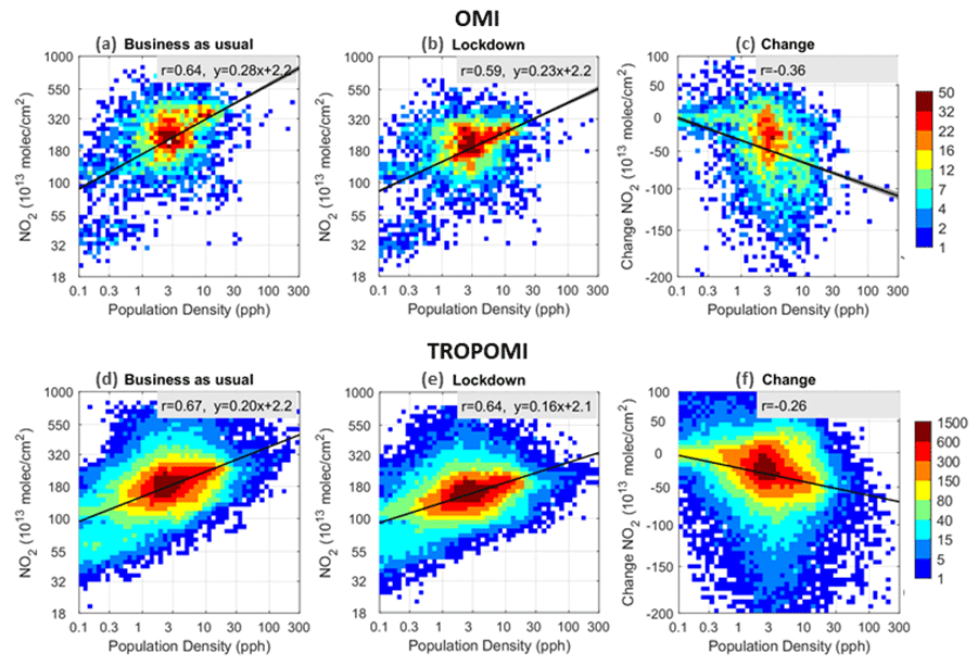
Figure 9Scatter density plot between the VCDtrop NO2 (×1013 molec. cm−2) and population density (pph) for the analysis period in different years. (a) Business as usual (BAU, 2016–2019) observed by OMI; (b) lockdown (LDN, 2020) observed by OMI; (c) changes (LDN − BAU) observed by OMI; (d) BAU (2019) observed by TROPOMI; (e) LDN (2020) observed by TROPOMI; (f) LND-BAU changes observed by TROPOMI. The linear best fit lines show the log–log relationship between VCDtrop NO2 (Y) and population density (X) given by equation , where y=log (Y), x=log (X) and c=log (C). Therefore, the equation can be written as or , where β is the slope of the line.
3.8 Linking the mobility change with NO2 change
In order to link the observed reduction in NO2 levels with the traffic emissions over the urban areas, Fig. 10 shows the 7 d moving average of the daily percentage change observed by OMI, TROPOMI, and CPCB across urban India from 1 March to 31 May 2020 against the Google mobility percentage reduction for three mobility categories: transit stations, workplace, and residential. Transit stations and workplace, proxies for traffic emissions (Forster et al., 2020), show a sharp decline (∼ 70 %) due to the lockdown. The signatures of reduced traffic can be seen even before the start of lockdown in mid-March 2020. The decrease in the workplaces resulted in the enhancement (25 %–30 %) of people at a residential location. The percentage reductions observed by satellites and surface monitoring are consistent with each other and follow the same trend of the workplaces and transit stations. The reductions observed by satellites and surface monitoring are ∼ 20 % lower than the reductions in workplaces and transit stations, which are compensated for by the enhancement in residential emissions. Surface (CPCB) measurements exhibit higher correlation (∼ 0.9 and 0.8, with and without moving average) with the mobility reduction compared to the satellite observation, which has a relatively weaker correlation (∼ 0.8 and 0.5). The positive correlation of NO2 reduction with workplaces and transit stations suggests that the reduction observed over the urban areas was linked with reduced traffic emissions due to travel restrictions for COVID-19 containment. Moreover, the mobility reduction was higher for larger cities as compared to the smaller ones (Fig. S6).
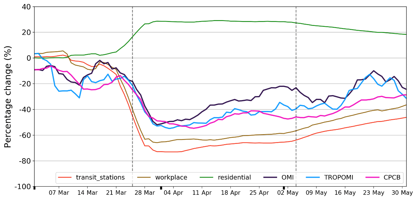
Figure 10Temporal evolution of estimated change (7 d rolling mean) of satellite-observed VCDtrop NO2 and surface-measured NO2 for the period 1 March–31 May 2020 from the baseline.
3.9 Limitations of this study
This study has few limitations that need to be considered while interpreting the results. The observed changes in the NO2 levels are the combined effect of changes in the emissions, local meteorology, large-scale dynamics, and non-linear chemistry. The variability in NO2, caused by weather patterns and non-linear chemistry is not included in the present work. Our study does not distinguish the differences in the upwind and downwind transport of plumes originating from urban areas and thermal power plants. Moreover, the estimates can be biased by the forest-fire plumes, which can be transported over a long distance. These limitations warrant a detailed modelling study to quantify the impact of long-range transport of plumes in the drastic reduction of urban emissions. One of the limitations arises due to the unavailability of the surface monitoring classification according to its location and vicinity of the local sources, which restricted a proper assessment of the space-based NO2 observation. To overcome this limitation, proper classification of the monitoring stations (Geiger et al., 2013) based on the environment type and vicinity of the sources will be helpful in air quality assessment.
The changes in NO2 levels over India during the COVID-19 lockdown (25 March–3 May 2020) have been studied using satellite-based VCDtrop NO2 observed by OMI and TROPOMI and surface NO2 concentrations obtained from CPCB. The changes between lockdown (LDN) and the same period during business-as-usual (BAU) years have been estimated over different land-use categories (e.g. urban, cropland, and forestland) across six geographical regions of India. Also, the changes observed from space and at the surface have been inter-compared, and the correlation with the population density has been studied.
Overall, a significant reduction in NO2 levels of up to ∼ 70 % was observed over India during the lockdown compared to the same period during BAU. The usual prominent NO2 hotspots observed by OMI and TROPOMI over urban agglomerations during BAU were barely noticeable during the lockdown. However, despite the reduction in electricity production, the coal-based thermal power plants continued to be major NO2 hotspots during the lockdown. Some of the largest reductions in NO2 were observed to be over the urban areas of the IGP region. The reduction observed for urban agglomerations was over 150 × 1013 molec. cm−2 (∼ 30 %) and even more for megacities showing a reduction of around 250 × 1013 molec. cm−2 (50 %). The reduction observed over the urban areas was linked with reduced traffic emissions due to travel restrictions for COVID-19 containment. The decrease was also observed over rural regions. Average declines of NO2 in the ranges of 14 %–30 %, 8 %–28 %, and 10 %–24 % were observed by OMI, and 22 %–27 %, 6 %–18 %, and 3 %–21 % were observed by TROPOMI over the urban, cropland, and forestland, respectively, in different regions of India. In contrast, an average enhancement over north-east India was observed due to positive fire anomalies during the lockdown. Although we have considered the grids with zero fire anomaly during the lockdown, the fire emissions can still enhance NO2 levels over grids with no fire activity because of horizontal transport.
The observed changes in VCDtrop NO2 were found to be spatially positively correlated with surface NO2 concentrations, indicating that the lockdown NO2 changes appear to be present in both measurement types. The TROPOMI NO2 showed a better correlation with surface NO2 and was more sensitive to the changes than the OMI because of the finer resolution. Therefore, TROPOMI can provide a better estimate of NO2 associated with fine-scale heterogeneous emissions. Also, VCDtrop NO2 was found to exhibit a good correlation with the population density, suggesting a strong dependence on the anthropogenic emissions. The changes observed in the VCDtrop NO2 during the lockdown were negatively correlated (i.e. reduction was positively correlated), with the population density suggesting a larger reduction for the densely populated cities. However, the influence of local emissions can be different in different cities.
The analysis presented in this work shows a significant change in NO2 levels across India. The observed reductions can be linked with the control measures taken to prevent the spread of the COVID-19 that restricted people's movement, resulting in a significant reduction in anthropogenic emissions. As an important message to policymakers, this study indicates the level of decrease in NO2 that is possible if dramatic reductions in key emission sectors such as road traffic were incorporated into air quality management strategies.
OMI data are available at the NASA Goddard Earth Sciences Data and Information Services Center (GESDISC) (https://disc.gsfc.nasa.gov/datasets/OMNO2d_003/summary, GESDISC, 2021). TROPOMI data are obtained from (http://www.temis.nl/airpollution/no2.php, TEMIS, 2020). Surface measured NO2 data across India are available at CPCB site (https://app.cpcbccr.com/ccr/, CPCB, 2020). VIIRS fire count data are available at the FIRMS web portal (https://firms.modaps.eosdis.nasa.gov/, FIRMS, 2020). India Population data used in this study are available at the https://www.worldpop.org/ (https://doi.org/10.5258/SOTON/WP00532, WorldPop., 2017). The LULC data for India are available at the Bhuvan, (https://bhuvan.nrsc.gov.in, Bhuvan, 2020) Indian Geo-Platform of Indian Space Research Organisation. ERA5 meteorology data are available at CDC (https://cds.climate.copernicus.eu/cdsapp, CDC, 2021). The mobility data are available on Google platform (https://www.google.com/covid19/mobility, Google, 2020).
The supplement related to this article is available online at: https://doi.org/10.5194/acp-21-5235-2021-supplement.
AB and VS conceived the study, analysed the data and interpreted the results with SS. MPC, SSD, RJP provided the processed TROPOMI data and provided useful discussion on satellite products. APK, KR, RSS, MPC, SSD, RJP, TS, SM provided useful discussion on the results. AB, VS, SS wrote the first draft and finalised the paper with input from all co-authors.
The authors declare that they have no conflict of interest.
The authors are thankful to the director, National Atmospheric Research Laboratory (NARL, India), for encouragement to conduct this research and provision of the necessary support. Akash Biswal and Shweta Singh greatly acknowledge the Ministry of Earth Sciences (MoES, India) for the research fellowship. We acknowledge and thank Central Pollution Control Board (CPCB), Ministry of Environment, Forest and Climate Change (MoEFCC, India) for making air quality data publicly available. We acknowledge Bhuvan, Indian Geo-Platform of Indian Space Research Organisation (ISRO), National Remote Sensing Centre (NRSC), for providing high-resolution LULC data. The authors gratefully acknowledge OMI, TROPOMI, and ERA5 science teams for making data publicly available. We also acknowledge the NASA Goddard Earth Sciences Data and Information Services Center, Tropospheric Emission Monitoring Internet Service and Climate Data Store. We also acknowledge Google community mobility data and report. We acknowledge support from the Air Pollution and Human Health for an Indian Megacity project PROMOTE funded by UK NERC and the Indian MOES (grant no. NE/P016391/1).
This research has been supported by the Natural Environment Research Council, UK (grant no. NE/P016391/1), and the Ministry of Earth Sciences, India.
This paper was edited by Andreas Hofzumahaus and reviewed by two anonymous referees.
Alonso-Blanco, E., Castro, A., Calvo, A. I., Pont, V., Mallet, M., and Fraile, R.: Wildfire smoke plumes transport under a subsidence inversion: Climate and health implications in a distant urban area, Sci. Total Environ., 619, 988–1002 2018.
Archer, C. L., Cervone, G., Golbazi, M., Al Fahel, N., and Hultquist, C.: Changes in air quality and human mobility in the USA during the COVID-19 pandemic, Bull. Atmospheric Sci. Technol., 1, 491–514, https://doi.org/10.1007/s42865-020-00019-0, 2020.
Barré, J., Petetin, H., Colette, A., Guevara, M., Peuch, V.-H., Rouil, L., Engelen, R., Inness, A., Flemming, J., Pérez García-Pando, C., Bowdalo, D., Meleux, F., Geels, C., Christensen, J. H., Gauss, M., Benedictow, A., Tsyro, S., Friese, E., Struzewska, J., Kaminski, J. W., Douros, J., Timmermans, R., Robertson, L., Adani, M., Jorba, O., Joly, M., and Kouznetsov, R.: Estimating lockdown induced European NO2 changes, Atmos. Chem. Phys. Discuss. [preprint], https://doi.org/10.5194/acp-2020-995, in review, 2020.
Bauwens, M., Compernolle, S., Stavrakou, T., Müller, J.-F., Gent, J. van, Eskes, H., Levelt, P. F., A, R. van der, Veefkind, J. P., Vlietinck, J., Yu, H., and Zehner, C.: Impact of Coronavirus Outbreak on NO2 Pollution Assessed Using TROPOMI and OMI Observations, Geophys. Res. Lett., 47, e2020GL087978, https://doi.org/10.1029/2020GL087978, 2020.
Bhuvan: Indian Geo-Platform of Indian Space Research Organisation, Thematic Services, available at: https://bhuvan.nrsc.gov.in, last access: 3 January 2020.
Biswal, A., Singh, T., Singh, V., Ravindra, K., and Mor, S.: COVID-19 lockdown and its impact on tropospheric NO2 concentrations over India using satellite-based data, Heliyon, 6, e04764, https://doi.org/10.1016/j.heliyon.2020.e04764, 2020.
Boersma, K. F., Eskes, H. J., and Brinksma, E. J.: Error analysis for tropospheric NO2 retrieval from space, J. Geophys. Res.-Atmos., 109, D04311, https://doi.org/10.1029/2003JD003962, 2004.
Boersma, K. F., Eskes, H. J., Dirksen, R. J., van der A, R. J., Veefkind, J. P., Stammes, P., Huijnen, V., Kleipool, Q. L., Sneep, M., Claas, J., Leitão, J., Richter, A., Zhou, Y., and Brunner, D.: An improved tropospheric NO2 column retrieval algorithm for the Ozone Monitoring Instrument, Atmos. Meas. Tech., 4, 1905–1928, https://doi.org/10.5194/amt-4-1905-2011, 2011.
CDC: Climate Data Store, ERA5 meteorology, available at: https://cds.climate.copernicus.eu/cdsapp, last access: 15 January 2021.
Celarier, E. A., Brinksma, E. J., Gleason, J. F., Veefkind, J. P., Cede, A., Herman, J. R., Ionov, D., Goutail, F., Pommereau, J.-P., Lambert, J.-C., Roozendael, M. van, Pinardi, G., Wittrock, F., Schönhardt, A., Richter, A., Ibrahim, O. W., Wagner, T., Bojkov, B., Mount, G., Spinei, E., Chen, C. M., Pongetti, T. J., Sander, S. P., Bucsela, E. J., Wenig, M. O., Swart, D. P. J., Volten, H., Kroon, M., and Levelt, P. F.: Validation of Ozone Monitoring Instrument nitrogen dioxide columns, J. Geophys. Res.-Atmos., 113, D15S15, https://doi.org/10.1029/2007JD008908, 2008.
Chan, K. L., Wiegner, M., van Geffen, J., De Smedt, I., Alberti, C., Cheng, Z., Ye, S., and Wenig, M.: MAX-DOAS measurements of tropospheric NO2 and HCHO in Munich and the comparison to OMI and TROPOMI satellite observations, Atmos. Meas. Tech., 13, 4499–4520, https://doi.org/10.5194/amt-13-4499-2020, 2020.
CPCB: Central Pollution Control Board, Central Control Room for Air Quality Management – All India, Surface measured NO2 data, available at: https://app.cpcbccr.com/ccr/, last access: 1 December 2020.
Curier, R. L., Kranenburg, R., Segers, A. J. S., Timmermans, R. M. A., and Schaap, M.: Synergistic use of OMI NO2 tropospheric columns and LOTOS–EUROS to evaluate the NOx emission trends across Europe, Remote Sens. Environ., 149, 58–69, https://doi.org/10.1016/j.rse.2014.03.032, 2014.
Duncan, B. N., Lamsal, L. N., Thompson, A. M., Yoshida, Y., Lu, Z., Streets, D. G., Hurwitz, M. M., and Pickering, K. E.: A space-based, high-resolution view of notable changes in urban NOx pollution around the world (2005–2014), J. Geophys. Res.-Atmos., 121, 976–996, https://doi.org/10.1002/2015JD024121, 2016.
Dutheil, F., Baker, J. S., and Navel, V.: COVID-19 as a factor influencing air pollution?, Environ. Pollut., 263, 114466, https://doi.org/10.1016/j.envpol.2020.114466, 2020.
Ekwaru, J. P. and Veugelers, P. J.: The overlooked importance of constants added in log transformation of independent variables with zero values: A proposed approach for determining an optimal constant, Stat. Biopharm. Res., 10, 26–29, 2018.
ESA: Air pollution drops in India following lockdown, available at: https://www.esa.int/Applications/Observing_the_Earth/Copernicus/Sentinel-5P/Air_pollution_drops_in_India_following_lockdown, last access: 1 October 2020.
Eskes, H., van Geffen, J., Boersma, F., Eichmann, K.-U., Apituley, A., Pedergnana, M., Sneep, M., Veefkind, J. P., and Loyola, D.: Sentinel-5 precursor/TROPOMI Level 2 Product User Manual Nitrogendioxide, Tech. Rep. S5P-KNMI-L2- 0021-MA, Koninklijk Nederlands Meteorologisch Instituut (KNMI), available at: https://sentinel.esa.int/documents/247904/2474726/Sentinel-5P-Level-2-Product-User-Manual-Nitrogen-Dioxide (last access: 20 December 2020), CI-7570-PUM, issue 3.0.0, 2019.
FIRMS (NASA Fire Information for Resource Management System): VIIRS fire count data, available at: https://firms.modaps.eosdis.nasa.gov/, last access: 25 December 2020.
Forster, P. M., Forster, H. I., Evans, M. J., Gidden, M. J., Jones, C. D., Keller, C. A., Lamboll, R. D., Quéré, C. L., Rogelj, J., Rosen, D., Schleussner, C.-F., Richardson, T. B., Smith, C. J., and Turnock, S. T.: Current and future global climate impacts resulting from COVID-19, Nat. Clim. Change, 10, 913–919, https://doi.org/10.1038/s41558-020-0883-0, 2020.
Gama, C., Relvas, H., Lopes, M., and Monteiro, A.: The impact of COVID-19 on air quality levels in Portugal: A way to assess traffic contribution, Environ. Res., 193, 110515, https://doi.org/10.1016/j.envres.2020.110515, 2020.
Geiger, J., Malherbe, L., Mathe, F., Ross-Jones, M., Sjoberg, K., Spangl, W., Stacey, B., Ortiz, A. G., de Leeuw, F., Borowiak, A., Galmarini, S., Gerboles, M., and de Saeger, E.: Assessment on siting criteria, classification and representativeness of air quality monitoring stations. JRC–AQUILA Position Paper, 2013, available at: https://ec.europa.eu/environment/air/pdf/SCREAM final.pdf (last access: 20 December 2020), 2013.
Georgoulias, A. K., van der A, R. J., Stammes, P., Boersma, K. F., and Eskes, H. J.: Trends and trend reversal detection in 2 decades of tropospheric NO2 satellite observations, Atmos. Chem. Phys., 19, 6269–6294, https://doi.org/10.5194/acp-19-6269-2019, 2019.
GESDISC (NASA Goddard Earth Sciences Data and Information Services Center): OMI/Aura NO2 Cloud-Screened Total and Tropospheric Column L3 Global Gridded 0.25 degree × 0.25 degree V3 (OMNO2d), available at: https://disc.gsfc.nasa.gov/datasets/OMNO2d_003/summary, last access: 1 January 2021.
Ghude, S. D., Fadnavis, S., Beig, G., Polade, S. D., and van der A, R. J.: Detection of surface emission hot spots, trends, and seasonal cycle from satellite-retrieved NO2 over India, J. Geophys. Res.-Atmos., 113, D20305, https://doi.org/10.1029/2007JD009615, 2008.
Ghude, S. D., Lal, D. M., Beig, G., van der A, R., and Sable, D.: Rain-Induced Soil NOx Emission From India During the Onset of the Summer Monsoon: A Satellite Perspective, J. Geophys. Res.-Atmos., 115, D16304, https://doi.org/10.1029/2009JD013367, 2010.
Ghude, S. D., Kulkarni, P. S., Kulkarni, S. H., Fadnavis, S. and A, R. J. V. D.: Temporal variation of urban NOx concentration in India during the past decade as observed from space, Int. J. Remote Sens., 32, 849–861, https://doi.org/10.1080/01431161.2010.517797, 2011.
Ghude, S. D., Kulkarni, S. H., Jena, C., Pfister, G. G., Beig, G., Fadnavis, S., and van der A, R. J.: Application of satellite observations for identifying regions of dominant sources of nitrogen oxides over the Indian Subcontinent, J. Geophys. Res.-Atmos., 118, 1075–1089, https://doi.org/10.1029/2012JD017811, 2013.
Goldberg, D. L., Anenberg, S. C., Griffin, D., McLinden, C. A., Lu, Z., and Streets, D. G.: Disentangling the impact of the COVID-19 lockdowns on urban NO2 from natural variability, Geophys. Res. Lett., 47, e2020GL089269, https://doi.org/10.1029/2020GL089269, 2020.
Google: LLC Community Mobility Reports, available at: https://www.google.com/covid19/mobility/, last access: December 2020.
Guenther, A. B., Jiang, X., Heald, C. L., Sakulyanontvittaya, T., Duhl, T., Emmons, L. K., and Wang, X.: The Model of Emissions of Gases and Aerosols from Nature version 2.1 (MEGAN2.1): an extended and updated framework for modeling biogenic emissions, Geosci. Model Dev., 5, 1471–1492, https://doi.org/10.5194/gmd-5-1471-2012, 2012.
Guttikunda, S. K., Nishadh, K. A., and Jawahar, P.: Air pollution knowledge assessments (APnA) for 20 Indian cities, Urban Clim., 27, 124–141, https://doi.org/10.1016/j.uclim.2018.11.005, 2019.
Guevara, M., Jorba, O., Soret, A., Petetin, H., Bowdalo, D., Serradell, K., Tena, C., Denier van der Gon, H., Kuenen, J., Peuch, V.-H., and Pérez García-Pando, C.: Time-resolved emission reductions for atmospheric chemistry modelling in Europe during the COVID-19 lockdowns, Atmos. Chem. Phys., 21, 773–797, https://doi.org/10.5194/acp-21-773-2021, 2021.
Hama, S. M. L., Kumar, P., Harrison, R. M., Bloss, W. J., Khare, M., Mishra, S., Namdeo, A., Sokhi, R., Goodman, P., and Sharma, C.: Four-year assessment of ambient particulate matter and trace gases in the Delhi-NCR region of India, Sustain. Cities Soc., 54, 102003, https://doi.org/10.1016/j.scs.2019.102003, 2020.
Hersbach, H., Bell, B., Berrisford, P., Hirahara, S., Horányi, A., Muñoz-Sabater, J., Nicolas, J., Peubey, C., Radu, R., Schepers, D., and Simmons, A.: The ERA5 global reanalysis, Q. J. Roy. Meteor. Soc., 146, 1999–2049, 2020.
Hilboll, A., Richter, A., and Burrows, J. P.: Long-term changes of tropospheric NO2 over megacities derived from multiple satellite instruments, Atmos. Chem. Phys., 13, 4145–4169, https://doi.org/10.5194/acp-13-4145-2013, 2013.
Hilboll, A., Richter, A., and Burrows, J. P.: NO2 pollution over India observed from space – the impact of rapid economic growth, and a recent decline, Atmos. Chem. Phys. Discuss. [preprint], https://doi.org/10.5194/acp-2017-101, in review, 2017.
Huang, G. and Sun, K.: Non-negligible impacts of clean air regulations on the reduction of tropospheric NO2 over East China during the COVID-19 pandemic observed by OMI and TROPOMI, Sci. Total Environ., 745, 141023, https://doi.org/10.1016/j.scitotenv.2020.141023, 2020.
ISFR: Indian State of forest Report, available at: https://fsi.nic.in (last access: 27 January 2021), 2019.
Kanniah, K. D., Kamarul Zaman, N. A. F., Kaskaoutis, D. G., and Latif, M. T.: COVID-19's impact on the atmospheric environment in the Southeast Asia region, Sci. Total Environ., 736, 139658, https://doi.org/10.1016/j.scitotenv.2020.139658, 2020.
Kramer, L. J., Leigh, R. J., Remedios, J. J., and Monks, P. S.: Comparison of OMI and ground-based in situ and MAX-DOAS measurements of tropospheric nitrogen dioxide in an urban area, J. Geophys. Res.-Atmos., 113, D16S39, https://doi.org/10.1029/2007JD009168, 2008.
Krotkov, N. A., Lamsal, L. N., Celarier, E. A., Swartz, W. H., Marchenko, S. V., Bucsela, E. J., Chan, K. L., Wenig, M., and Zara, M.: The version 3 OMI NO2 standard product, Atmos. Meas. Tech., 10, 3133–3149, https://doi.org/10.5194/amt-10-3133-2017, 2017.
Krotkov, N. A., Lamsal, L. N., Marchenko, S. V., and Swartz, W. H.: OMNO2 README Document Data Product Version 4.0, December 2019, Document Version 9.0, available at: https://acdisc.gesdisc.eosdis.nasa.gov/data/Aura_OMI_Level3/OMNO2d.003/doc/README.OMNO2.pdf (last access: 22 January 2021, login required), 2019.
Lamsal, L. N., Martin, R. V., Donkelaar, A. van, Celarier, E. A., Bucsela, E. J., Boersma, K. F., Dirksen, R., Luo, C., and Wang, Y.: Indirect validation of tropospheric nitrogen dioxide retrieved from the OMI satellite instrument: Insight into the seasonal variation of nitrogen oxides at northern midlatitudes, J. Geophys. Res.-Atmos., 115, D05302, https://doi.org/10.1029/2009JD013351, 2010.
Lamsal, L. N., Martin, R. V., Parrish, D. D., and Krotkov, N. A.: Scaling Relationship for NO2 Pollution and Urban Population Size: A Satellite Perspective, Environ. Sci. Technol., 47, 7855–7861, https://doi.org/10.1021/es400744g, 2013.
Lamsal, L. N., Duncan, B. N., Yoshida, Y., Krotkov, N. A., Pickering, K. E., Streets, D. G., and Lu, Z.: U.S. NO2 trends (2005–2013): EPA Air Quality System (AQS) data versus improved observations from the Ozone Monitoring Instrument (OMI), Atmos. Environ., 110, 130–143, https://doi.org/10.1016/j.atmosenv.2015.03.055, 2015.
Lamsal, L. N., Krotkov, N. A., Vasilkov, A., Marchenko, S., Qin, W., Yang, E.-S., Fasnacht, Z., Joiner, J., Choi, S., Haffner, D., Swartz, W. H., Fisher, B., and Bucsela, E.: Ozone Monitoring Instrument (OMI) Aura nitrogen dioxide standard product version 4.0 with improved surface and cloud treatments, Atmos. Meas. Tech., 14, 455–479, https://doi.org/10.5194/amt-14-455-2021, 2021.
Lane, T. E., Donahue, N. M., and Pandis, S. N.: Effect of NOx on Secondary Organic Aerosol Concentrations, Environ. Sci. Technol., 42, 6022–6027, https://doi.org/10.1021/es703225a, 2008.
Li, F., Zhang, X., Kondragunta, S., and Csiszar, I.: Comparison of Fire Radiative Power Estimates From VIIRS and MODIS Observations, J. Geophys. Res.-Atmos., 123, 4545–4563, https://doi.org/10.1029/2017JD027823, 2018.
Lin, J.-T., Liu, M.-Y., Xin, J.-Y., Boersma, K. F., Spurr, R., Martin, R., and Zhang, Q.: Influence of aerosols and surface reflectance on satellite NO2 retrieval: seasonal and spatial characteristics and implications for NOx emission constraints, Atmos. Chem. Phys., 15, 11217–11241, https://doi.org/10.5194/acp-15-11217-2015, 2015.
Liu, F., Page, A., Strode, S. A., Yoshida, Y., Choi, S., Zheng, B., Lamsal, L. N., Li, C., Krotkov, N. A., Eskes, H., A, R. van der, Veefkind, P., Levelt, P. F., Hauser, O. P., and Joiner, J.: Abrupt decline in tropospheric nitrogen dioxide over China after the outbreak of COVID-19, Sci. Adv., 6, eabc2992, https://doi.org/10.1126/sciadv.abc2992, 2020.
Mahajan, A. S., De Smedt, I., Biswas, M. S., Ghude, S., Fadnavis, S., Roy, C., and van Roozendael, M.: Inter-annual variations in satellite observations of nitrogen dioxide and formaldehyde over India, Atmos. Environ., 116, 194–201, https://doi.org/10.1016/j.atmosenv.2015.06.004, 2015.
Mahato, S., Pal, S., and Ghosh, K. G.: Effect of lockdown amid COVID-19 pandemic on air quality of the megacity Delhi, India, Sci. Total Environ., 730, 139086, https://doi.org/10.1016/j.scitotenv.2020.139086, 2020.
Martin, R. V., Sioris, C. E., Chance, K., Ryerson, T. B., Bertram, T. H., Wooldridge, P. J., Cohen, R. C., Neuman, J. A., Swanson, A. and Flocke, F. M.: Evaluation of space-based constraints on global nitrogen oxide emissions with regional aircraft measurements over and downwind of eastern North America, J. Geophys. Res.-Atmos., 111, D15308, https://doi.org/10.1029/2005JD006680, 2006.
Mebust, A. K., Russell, A. R., Hudman, R. C., Valin, L. C., and Cohen, R. C.: Characterization of wildfire NOx emissions using MODIS fire radiative power and OMI tropospheric NO2 columns, Atmos. Chem. Phys., 11, 5839–5851, https://doi.org/10.5194/acp-11-5839-2011, 2011.
MHA (No.40-3/2020-DM-I (A)): Government of India, Ministry of Home Affairs, available at: https://www.mha.gov.in/sites/default/files/MHA order dt 15.04.2020, with Revised Consolidated Guidelines_compressed (3).pdf, http://www.du.ac.in/du/uploads/PR_Consolidated Guideline of MHA_28032020 (1)_1.PDF, https://mha.gov.in/sites/default/files/MHA Order Dt. 1.5.2020 to extend Lockdown period for 2 weeks w.e.f. 4.5.2020 with new guidelines.pdf, last access: 1 October 2020.
Mills, I. C., Atkinson, R. W., Kang, S., Walton, H., and Anderson, H. R.: Quantitative systematic review of the associations between short-term exposure to nitrogen dioxide and mortality and hospital admissions, BMJ Open, 5, e006946, https://doi.org/10.1136/bmjopen-2014-006946, 2015.
Monks, P. S., Archibald, A. T., Colette, A., Cooper, O., Coyle, M., Derwent, R., Fowler, D., Granier, C., Law, K. S., Mills, G. E., Stevenson, D. S., Tarasova, O., Thouret, V., von Schneidemesser, E., Sommariva, R., Wild, O., and Williams, M. L.: Tropospheric ozone and its precursors from the urban to the global scale from air quality to short-lived climate forcer, Atmos. Chem. Phys., 15, 8889–8973, https://doi.org/10.5194/acp-15-8889-2015, 2015.
Muhammad, S., Long, X., and Salman, M.: COVID-19 pandemic and environmental pollution: A blessing in disguise?, Sci. Total Environ., 728, 138820, https://doi.org/10.1016/j.scitotenv.2020.138820, 2020.
Naeger, A. R. and Murphy, K.: Impact of COVID-19 Containment Measures on Air Pollution in California, Aerosol Air Qual. Res., 20, 2025–2034, https://doi.org/10.4209/aaqr.2020.05.0227, 2020.
Navinya, C., Patidar, G., and Phuleria, H. C.: Examining Effects of the COVID-19 National Lockdown on Ambient Air Quality across Urban India, Aerosol Air Qual. Res., 20, 1759–1771, https://doi.org/10.4209/aaqr.2020.05.0256, 2020.
Nori-Sarma, A., Thimmulappa, R. K., Venkataramana, G. V., Fauzie, A. K., Dey, S. K., Venkareddy, L. K., Berman, J. D., Lane, K. J., Fong, K. C., Warren, J. L., and Bell, M. L.: Low-cost NO2 monitoring and predictions of urban exposure using universal kriging and land-use regression modelling in Mysore, India, Atmos. Environ., 226, 117395, https://doi.org/10.1016/j.atmosenv.2020.117395, 2020.
NRSC: National Remote Sensing Centre, Natural Resources Census, National Land Use and Land Cover Mapping Using Multitemporal AWiFS Data (LULC-AWiFS), Eighth Cycle (2011–12) Indian Space Research Organisation Department of Space, Government of India, available at: https://bhuvan-app1.nrsc.gov.in/2dresources/thematic/LULC250/1112.pdf (last access: 1 October 2020), 2012.
Pathakoti, M., Muppalla, A., Hazra, S., Dangeti, M., Shekhar, R., Jella, S., Mullapudi, S. S., Andugulapati, P., and Vijayasundaram, U.: An assessment of the impact of a nation-wide lockdown on air pollution – a remote sensing perspective over India, Atmos. Chem. Phys. Discuss. [preprint], https://doi.org/10.5194/acp-2020-621, 2020.
Penn, E. and Holloway, T.: Evaluating current satellite capability to observe diurnal change in nitrogen oxides in preparation for geostationary satellite missions, Environ. Res. Lett., 15, 034038, https://doi.org/10.1088/1748-9326/ab6b36, 2020.
Pope, R. J., Arnold, S. R., Chipperfield, M. P., Latter, B. G., Siddans, R., and Kerridge, B. J.: Widespread changes in UK air quality observed from space, Atmos. Sci. Lett., 19, e817, https://doi.org/10.1002/asl.817, 2018.
POSOCO: Power system operation corporation limited, monthly statistical report, available at: https://posoco.in/reports/monthly-reports/monthly-reports-2020-21/, last access: 15 January 2021.
Prasad, A. K., Singh, R. P., and Kafatos, M.: Influence of coal-based thermal power plants on the spatial–temporal variability of tropospheric NO2column over India, Environ. Monit. Assess., 184, 1891–1907, https://doi.org/10.1007/s10661-011-2087-6, 2012.
Prosperi, P., Bloise, M., Tubiello, F. N., Conchedda, G., Rossi, S., Boschetti, L., Salvatore, M., and Bernoux, M.: New estimates of greenhouse gas emissions from biomass burning and peat fires using MODIS Collection 6 burned areas, Clim. Change, 161, 415–432, https://doi.org/10.1007/s10584-020-02654-0, 2020.
Russell, A. R., Valin, L. C., and Cohen, R. C.: Trends in OMI NO2 observations over the United States: effects of emission control technology and the economic recession, Atmos. Chem. Phys., 12, 12197–12209, https://doi.org/10.5194/acp-12-12197-2012, 2012.
Sahu, L. K., Sheel, V., Pandey, K., Yadav, R., Saxena, P., and Gunthe, S.: Regional biomass burning trends in India: Analysis of satellite fire data, J. Earth Syst. Sci., 124, 1377–1387, https://doi.org/10.1007/s12040-015-0616-3, 2015.
Schroeder, W., Oliva, P., Giglio, L., and Csiszar, I. A.: The New VIIRS 375m active fire detection data product: Algorithm description and initial assessment, Remote Sens. Environ., 143, 85–96, https://doi.org/10.1016/j.rse.2013.12.008, 2014.
Sharma, P., Sharma, P., Jain, S., and Kumar, P.: An integrated statistical approach for evaluating the exceedence of criteria pollutants in the ambient air of megacity Delhi, Atmos. Environ., 70, 7–17, https://doi.org/10.1016/j.atmosenv.2013.01.004, 2013.
Sharma, S., Zhang, M., Anshika, Gao, J., Zhang, H., and Kota, S. H.: Effect of restricted emissions during COVID-19 on air quality in India, Sci. Total Environ., 728, 138878, https://doi.org/10.1016/j.scitotenv.2020.138878, 2020.
Siddiqui, A., Halder, S., Chauhan, P., and Kumar, P.: COVID-19 Pandemic and City-Level Nitrogen Dioxide (NO2) Reduction for Urban Centres of India, J. Indian Soc. Remote Sens., 48, 999–1006, https://doi.org/10.1007/s12524-020-01130-7, 2020.
Shi, Z., Song, C., Liu, B., Lu, G., Xu, J., Vu, T. V., Elliott, R. J. R., Li, W., Bloss, W. J., and Harrison, R. M.: Abrupt but smaller than expected changes in surface air quality attributable to COVID-19 lockdowns, Sci. Adv., 7, eabd6696, https://doi.org/10.1126/sciadv.abd6696, 2021.
Siddiqui, A., Halder, S., Chauhan, P., and Kumar, P.: COVID-19 Pandemic and City-Level Nitrogen Dioxide (NO2) Reduction for Urban Centres of India, J. Indian Soc. Remote Sens., 48, 999–1006, https://doi.org/10.1007/s12524-020-01130-7, 2020.
Singh, V., Singh, S., Biswal, A., Kesarkar, A. P., Mor, S., and Ravindra, K.: Diurnal and temporal changes in air pollution during COVID-19 strict lockdown over different regions of India, Environ. Pollut., 266, 115368, https://doi.org/10.1016/j.envpol.2020.115368, 2020.
Solomon, S., Qin, D., Manning, M., Marquis, M., Averyt, K., Tignor, M. M. B., LeRoy Miller, H. J., and Chen, Z.: Climate Change 2007: 10Working Group I: The Physical Science Basis, Tech. rep., Intergovernmental Panel on Climate Change, Geneva, 2007.
Stevens, F. R., Gaughan, A. E., Linard, C., and Tatem, A. J.: Disaggregating Census Data for Population Mapping Using Random Forests with Remotely-Sensed and Ancillary Data, PLOS ONE, 10, e0107042, https://doi.org/10.1371/journal.pone.0107042, 2015.
TEMIS (Tropospheric Emission Monitoring Internet Service): Tropospheric NO2 from satellites, TROPOMI (S5-p), available at: http://www.temis.nl/airpollution/no2.php, last access: 1 December 2020.
Tobías, A., Carnerero, C., Reche, C., Massagué, J., Via, M., Minguillón, M. C., Alastuey, A., and Querol, X.: Changes in air quality during the lockdown in Barcelona (Spain) one month into the SARS-CoV-2 epidemic, Sci. Total Environ., 726, 138540, https://doi.org/10.1016/j.scitotenv.2020.138540, 2020.
ul-Haq, Z., Tariq, S., Ali, M., Rana, A. D., and Mahmood, K.: Satellite-sensed tropospheric NO2 patterns and anomalies over Indus, Ganges, Brahmaputra, and Meghna river basins, Int. J. Remote Sens., 38, 1423–1450, https://doi.org/10.1080/01431161.2017.1283071, 2017.
USEPA and CATC (Clean Air Technology Center): Nitrogen oxides (NOx) why and how they are controlled, Diane Publishing, available at: https://www3.epa.gov/ttncatc1/dir1/fnoxdoc.pdf (last access: 20 December 2020), 1999.
van der A, R. J., Eskes, H. J., Boersma, K. F., Noije, T. P. C. van, Roozendael, M. V., Smedt, I. D., Peters, D. H. M. U., and Meijer, E. W.: Trends, seasonal variability and dominant NOx source derived from a ten year record of NO2 measured from space, J. Geophys. Res.-Atmos., 113, https://doi.org/10.1029/2007JD009021, 2008.
van Geffen, J. H. G. M., Eskes, H. J., Boersma, K. F., Maasakkers, J. D., and Veefkind, J. P.: TROPOMI ATBD of the total and tropospheric NO2 data products, Report S5P-KNMI-L2-0005-RP, version 2.1.0, to be released, KNMI, De Bilt, the Netherlands, available at: http://www.tropomi.eu/documents/atbd/ (last access: 10 September 2020), 2019.
van Geffen, J., Boersma, K. F., Eskes, H., Sneep, M., ter Linden, M., Zara, M., and Veefkind, J. P.: S5P TROPOMI NO2 slant column retrieval: method, stability, uncertainties and comparisons with OMI, Atmos. Meas. Tech., 13, 1315–1335, https://doi.org/10.5194/amt-13-1315-2020, 2020.
Veefkind, J. P., Aben, I., McMullan, K., Förster, H., de Vries, J., Otter, G., Claas, J., Eskes, H. J., de Haan, J. F., Kleipool, Q., van Weele, M., Hasekamp, O., Hoogeveen, R., Landgraf, J., Snel, R., Tol, P., Ingmann, P., Voors, R., Kruizinga, B., Vink, R., Visser, H., and Levelt, P. F.: TROPOMI on the ESA Sentinel-5 Precursor: A GMES mission for global observations of the atmospheric composition for climate, air quality and ozone layer applications, Remote Sens. Environ., 120, 70–83, https://doi.org/10.1016/j.rse.2011.09.027, 2012.
Venkataraman, C., Habib, G., Kadamba, D., Shrivastava, M., Leon, J.-F., Crouzille, B., Boucher, O., and Streets, D. G.: Emissions from open biomass burning in India: Integrating the inventory approach with high-resolution Moderate Resolution Imaging Spectroradiometer (MODIS) active-fire and land cover data, Global Biogeochem. Cy., 20, GB2013, https://doi.org/10.1029/2005GB002547, 2006.
Venter, Z. S., Aunan, K., Chowdhury, S., and Lelieveld, J.: COVID-19 lockdowns cause global air pollution declines, P. Natl. Acad. Sci., 117, 18984–18990, https://doi.org/10.1073/pnas.2006853117, 2020.
Wang, C., Wang, T., Wang, P., and Rakitin, V.: Comparison and Validation of TROPOMI and OMI NO2 Observations over China, Atmosphere, 11, 636, https://doi.org/10.3390/atmos11060636, 2020.
WorldPop.: India 100m Population, Version 2, University of Southampton, https://doi.org/10.5258/SOTON/WP00532, https://www.worldpop.org/ (last access: 30 June 2020), 2017.
Yarragunta, Y., Srivastava, S., Mitra, D., and Chandola, H. C.: Influence of forest fire episodes on the distribution of gaseous air pollutants over Uttarakhand, India, GIScience Remote Sens., 57, 190–206, https://doi.org/10.1080/15481603.2020.1712100, 2020.