the Creative Commons Attribution 4.0 License.
the Creative Commons Attribution 4.0 License.
 | 31 Mar 2021
Constraints on global aerosol number concentration, SO2 and condensation sink in UKESM1 using ATom measurements
Ananth Ranjithkumar
Christina Williamson
Andrew Rollins
Kirsty Pringle
Agnieszka Kupc
Nathan Luke Abraham
Charles Brock
Ken Carslaw
Understanding the vertical distribution of aerosol helps to reduce the uncertainty in the aerosol life cycle and therefore in the estimation of the direct and indirect aerosol forcing. To improve our understanding, we use measurements from four deployments of the Atmospheric Tomography (ATom) field campaign (ATom1–4) which systematically sampled aerosol and trace gases over the Pacific and Atlantic oceans with near pole-to-pole coverage. We evaluate the UK Earth System Model (UKESM1) against ATom observations in terms of joint biases in the vertical profile of three variables related to new particle formation: total particle number concentration (NTotal), sulfur dioxide (SO2) mixing ratio and the condensation sink. The NTotal, SO2 and condensation sink are interdependent quantities and have a controlling influence on the vertical profile of each other; therefore, analysing them simultaneously helps to avoid getting the right answer for the wrong reasons. The simulated condensation sink in the baseline model is within a factor of 2 of observations, but the NTotal and SO2 show much larger biases mainly in the tropics and high latitudes. We performed a series of model sensitivity tests to identify atmospheric processes that have the strongest influence on overall model performance. The perturbations take the form of global scaling factors or improvements to the representation of atmospheric processes in the model, for example by adding a new boundary layer nucleation scheme. In the boundary layer (below 1 km altitude) and lower troposphere (1–4 km), inclusion of a boundary layer nucleation scheme (Metzger et al., 2010) is critical to obtaining better agreement with observations. However, in the mid (4–8 km) and upper troposphere (> 8 km), sub-3 nm particle growth, pH of cloud droplets, dimethyl sulfide (DMS) emissions, upper-tropospheric nucleation rate, SO2 gas-scavenging rate and cloud erosion rate play a more dominant role. We find that perturbations to boundary layer nucleation, sub-3 nm growth, cloud droplet pH and DMS emissions reduce the boundary layer and upper tropospheric model bias simultaneously. In a combined simulation with all four perturbations, the SO2 and condensation sink profiles are in much better agreement with observations, but the NTotal profile still shows large deviations, which suggests a possible structural issue with how nucleation or gas/particle transport or aerosol scavenging is handled in the model. These perturbations are well-motivated in that they improve the physical basis of the model and are suitable for implementation in future versions of UKESM.
- Article
(14090 KB) - Full-text XML
- BibTeX
- EndNote


Aerosols affect the global energy balance directly by scattering and absorbing solar radiation and indirectly by their ability to act as cloud condensation nuclei (CCN), which changes the microphysical properties of clouds (Albrecht, 1989; Twomey, 1977). The direct and indirect effects aerosols have on climate have been identified as the largest source of uncertainty in the assessment of anthropogenic forcing (Bellouin et al., 2020; Carslaw et al., 2013; Myhre et al., 2013). The direct radiative forcing by aerosol particles is dependent on the scattering and absorption of solar radiation, which in turn is dependent on aerosol properties like their size, shape and refractive index. The indirect radiative forcing is dependent on aerosol particles forming or behaving as CCN (or ice nuclei), which is controlled by the hygroscopicity and aerosol size distribution at cloud base (1–3 km). There are still gaps in our knowledge of atmospheric processes that control the spatial, temporal and size distribution of aerosols in the atmosphere. Atmospheric aerosol concentrations depend on their sources; primary (emissions) and secondary (new particle formation and particle growth), their sinks (scavenging, wet and dry deposition) and transport through the atmosphere (Merikanto et al., 2009). Thus, the different atmospheric processes that have a controlling influence on the aerosol distribution throughout the atmosphere must be better understood.
Global-scale measurements of aerosol microphysical properties are needed to evaluate general circulation models (GCMs). Satellite measurements have extensive global coverage, but they cannot detect particles smaller than about 100 nm diameter. In situ aircraft measurements give more detailed information about the full size distribution, chemical composition and radiative properties of aerosol particles. In past studies (Dunne et al., 2016; Ekman et al., 2012; Watson-Parris et al., 2019) global models have been compared against measurement campaigns such as CARIBIC (Civil Aircraft for Regular Investigation of the Atmosphere Based on an Instrument) (Heintzenberg et al., 2011), ACE1 (First Aerosol Characterization Experiment) (Clarke et al., 1998), PEM Tropics (Pacific Exploratory missions – Tropics) (Clarke et al., 1999), ARCTAS (Arctic Research of the Composition of the Troposphere from Aircraft and Satellites) (Jacob et al., 2010), PASE (Pacific Atmosphere Sulphur Experiment) (Faloona et al., 2009), INTEX-A (Intercontinental chemistry transport experiment – North America) (Singh et al., 2006) and VOCALS (VAMOS Ocean-Cloud-Atmosphere-Land Study) (Wood et al., 2011). Each of these campaigns had goals to help us understand particle size distribution in the upper troposphere, the particle production rate in cloud outflow regions, Arctic atmospheric composition, sulfur processing, tropospheric composition over land and clouds/precipitation in the south-eastern Pacific respectively. The measurements from these campaigns were used to identify atmospheric processes that help constrain the particle size distribution in global climate models like MIT-CAM3 (Ekman et al., 2012) and ECHAM-HAM (Watson-Parris et al., 2019) with observations.
In this work, we compare in situ aircraft observations conducted as part of the NASA Atmospheric Tomography Mission (ATom) (Wofsy et al., 2018) to a global climate model (UK Earth System Model, UKESM1) to better quantify the model biases in particle number concentration, SO2 and the condensation sink. The ATom campaigns provide a representative continuous dataset of daytime aerosol, gas and radical concentrations and properties by continuously sampling the atmosphere vertically and spatially over a vast region of the marine-free troposphere. This single global dataset was obtained between 2016 and 2018 during four campaigns sampling each of the four seasons. During these campaigns, a large aerosol and gas instrument payload was deployed on the NASA DC-8 aircraft for systematic sampling of the atmosphere spanning altitudes between 0.2 and 12 km, and spatially it encompasses the Pacific and Atlantic oceans with near pole-to-pole coverage. These data have been used recently (Williamson et al., 2019) to highlight the importance of new particle formation to CCN concentration in the upper and free troposphere and to highlight severe deficiencies in the ability of state-of-the-art global chemistry climate models to capture new particle formation, particle growth and aerosol vertical transport accurately.
The ATom data have also been used in previous work to address biases in the vertical profile of sea salt and black carbon in the Community Earth System Model (CESM) and to better understand the in-cloud removal of aerosols by deep convection (Yu et al., 2019). Black carbon lifetime and differences in black carbon loading between the Pacific and Atlantic basins have also been researched using ATom measurements (Katich et al., 2018; Lund et al., 2018). Other studies used the measurements to address uncertainties associated with the life cycle of organic aerosol in the remote troposphere (Hodzic et al., 2020) and to investigate the mechanisms of new particle formation in the tropical upper troposphere (Kupc et al., 2020). The measurements have also shed light on the global distribution of biomass-burning aerosol (Schill et al., 2020), brown carbon (Zeng et al., 2020) and DMS oxidation chemistry (Veres et al., 2020).
Although the ATom dataset is extensive and provides important information about aerosol number and gas concentrations (Williamson et al., 2019; Wofsy et al., 2018), there are some challenges when comparing it to a GCM. A single data point sampled represents a point in the atmosphere defined by the latitude, longitude, altitude and time the data were collected. The UKESM output is, however, an average over a broad horizontal grid box of ∼ 135 km across, and it is usually temporally averaged over a month. In previous studies (Lund et al., 2018; Samset et al., 2018; Schutgens et al., 2016) it has been shown that sampling errors can be minimised by averaging the observations over time, and model errors can be reduced by using 4D model fields with high temporal resolution. In the first part of this paper, we evaluate UKESM at 3-hourly time resolution against observations and highlight some of the biases that exist in the model in different regions of Earth.
In the second part of this paper, we focus on trying to understand and reduce these biases. We focus on processes related to new particle formation, as this is the dominant source of aerosol number concentration globally (Gordon et al., 2017; Yu and Luo, 2009). Some model developments and a series of sensitivity simulations are performed to determine the source of the model–measurement bias. As well as resolving a bug in the model, we also address some of the deficiencies in the nucleation-mode microphysics and the dependence of coagulation sink on particle diameter. The sensitivity tests comprise model simulations in which we perturb various parameters that control different atmospheric processes, one at a time.
In order to obtain physically motivated reductions in model bias, we evaluate the model simultaneously against three observed quantities related to new particle formation: total particle number concentration (NTotal), SO2 mixing ratio and condensation sink. The condensation sink is a measure of how rapidly condensable vapour molecules (in UKESM, sulfuric acid and secondary organic aerosol material) and newly formed molecular clusters are removed by the existing aerosol surface area. It is a loss term for new particles, while SO2 is effectively a production term because it controls sulfuric acid vapour concentrations. Assessing the influence of model processes on only one of these quantities in one-at-a-time sensitivity tests can result in misleading or incomplete conclusions about model performance, because different atmospheric processes affect NTotal, SO2 and the condensation sink to varying degrees and can be independent of each other. As an example, an atmospheric process like in-cloud production of sulfate aerosol can increase the condensation sink, which will decrease the gas concentration of precursors such as sulfuric acid, H2SO4, for new particle formation and then in turn decrease NTotal. Perturbing atmospheric processes can also have a direct effect on the SO2 mixing ratio and affect H2SO4 concentration, which controls new particle formation (NPF), and we know from past studies (Gordon et al., 2017) that new particle formation is the source of about half of the CCN in the atmosphere. Improving the model–observation match to only one of NTotal, SO2 and the condensation sink can result in a poorer match for the other two quantities. Therefore, it is important to identify atmospheric processes that reduce NTotal, SO2 and condensation sink biases simultaneously.
The main goal of the ATom campaign was to improve our scientific understanding of the chemistry and climate processes in the remote atmosphere over marine regions. In relation to aerosols, the campaign helps to quantify the abundance, distribution, composition and optical properties of aerosol particles in the remote atmosphere. This can help determine the source of these particles and evaluate the mechanism for formation and growth of new particles to form CCN. The whole campaign used the NASA DC-8 research aircraft and was subdivided into four series of flights, ATom1 (August–September 2016), ATom2 (January–February 2017), ATom3 (September–October 2017) and ATom4 (April–May 2018). The flight path for each of the ATom deployments is shown in Fig. 1. Measurements were made between ∼ 0.18 and ∼ 12 km altitude, from the Antarctic to the Arctic, over the Atlantic and Pacific oceans. All of the data are publicly available (Wofsy et al., 2018).
We used the SO2 data from ATom4 (the SO2 data from ATom1 to 3 were not sensitive at concentrations less than 100 ppt) and the particle number concentration data from ATom1, ATom2, ATom3 and ATom4. The instruments used to measure the aerosol size distribution from 2.7 nm to 4.8 µm are a nucleation-mode aerosol size spectrometer (NMASS) (Williamson et al., 2018), an ultra-high-sensitivity aerosol size spectrometer (UHSAS) and a laser aerosol spectrometer (LAS). The NMASS consists of five continuous laminar flow condensation particle counters (CPCs) in parallel, with each CPC operated at different settings so as to detect different size classes (Brock et al., 2019; Williamson et al., 2018). During ATom1, the cut-off sizes (the probability of the particles at cut-off size of being detected is greater than 50 %) for each of the CPCs were 3.2, 8.3, 14, 27 and 59 nm. From ATom2 to ATom4 (more CPCs were present in addition to the CPCs from ATom1), additional cut-off sizes of 5.2, 6.9, 11, 20 and 38 nm were present. This setup helps establish the aerosol size distribution for particles smaller than 59 nm. The UHSAS measures particle number concentrations for particles with diameter between 63 and 1000 nm (Kupc et al., 2018). The LAS efficiently measures particles between 120 nm and 4.8 µm. The POPS instrument was operated as a backup to detect coarse-mode particles (Gao et al., 2016).
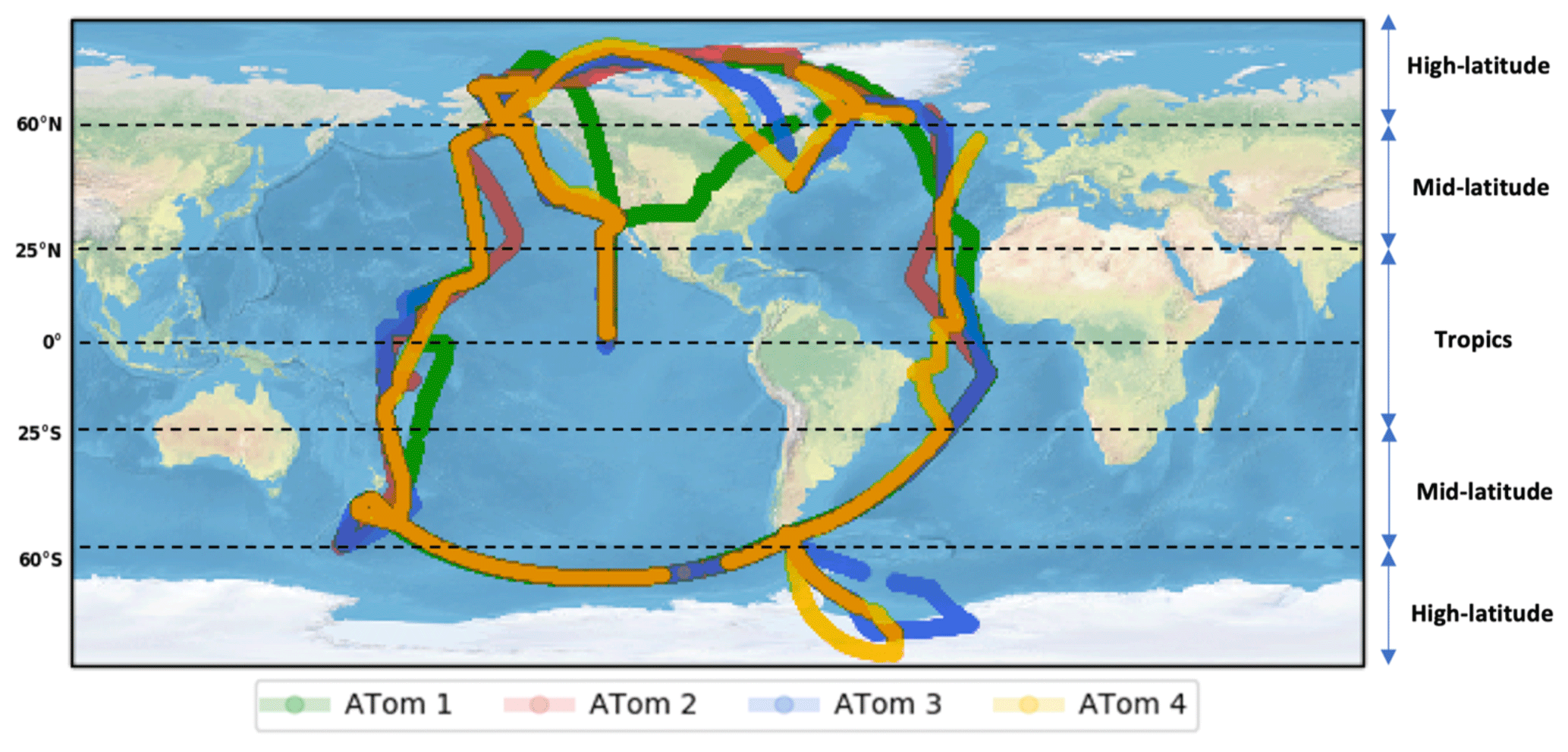
Figure 1Flight tracks for NASA DC-8 for the four ATom campaigns: ATom1 (August–September 2016, green), ATom2 (January–February 2017, red), ATom3 (September–October 2017, blue) and ATom4 (April–May 2018, yellow).
The SO2 measurements were obtained using the laser-induced fluorescence instrument (Rollins et al., 2016). SO2 mixing ratios at high altitudes are quite low (between 1 and 10 parts per trillion). It is difficult to measure the SO2 mixing ratio at low pressure with high precision. This instrument is capable of retrieving precise measurements of SO2 concentration at pressures as low as 35 hPa, making this instrument operable up to altitudes of 20 km. The instrument has a detection limit of 2 ppt (at a 10 s measurement interval) and an overall uncertainty of ± (16 % + 0.9 ppt).
The model used in this work is UKESM1 (Mulcahy et al., 2020; Sellar et al., 2019) in its atmosphere-only configuration (with fixed sea surface temperatures and prescribed biogenic emissions from a fully coupled model simulation). The latest HadGEM3 global coupled (GC) climate configuration of the UK Met Office was used to develop UKESM. HadGEM3 consists of the core physical dynamical processes of the atmosphere, land, ocean and sea ice systems (Ridley et al., 2018; Storkey et al., 2018; Walters et al., 2017). The UK's contribution to the Coupled Model Intercomparison Project Phase 6 (CMIP 6) (Eyring et al., 2016) is comprised of model simulations from the HadGEM3 and UKESM1 models.
Atmospheric composition is simulated with the chemistry-aerosol component of UKESM, which is the UK Chemistry and Aerosol model (UKCA) (Morgenstern et al., 2009; O'Connor et al., 2014; Archibald et al., 2020). The anthropogenic, biomass-burning, biogenic and DMS land emissions used by the model are taken from Hoesly et al. (2018), van Marle et al. (2017), Sindelarova et al. (2014) and Spiro et al. (1992) respectively. The aerosol scheme within UKCA is referred to as the Global Model of Aerosol Processes, GLOMAP mode (Mann et al., 2010; Mulcahy et al., 2020). It uses a two-moment pseudo-modal approach and simulates multicomponent global aerosol, which includes sulfate, black carbon, organic matter and sea spray. Dust is simulated separately using a difference scheme (Woodward, 2001). GLOMAP mode includes aerosol microphysical processes of new particle formation, condensation, coagulation, wet scavenging, dry deposition and cloud processing. The aerosol particle size distribution is represented using five log-normal modes, nucleation soluble, Aitken soluble, accumulation soluble, coarse soluble and Aitken insoluble, with their size ranges shown in Table A1 (Appendix A). UKCA is coupled to other modules in UKESM to handle tracer transport by convection, advection and boundary layer mixing. Originally in GLOMAP mode, sulfate and secondary organic formation was driven by prescribed oxidant fields (Mann et al., 2010). However, in this study the UKCA chemistry and aerosol modules are fully coupled (Mulcahy et al., 2020).
The model can be run in different configurations (Walters et al., 2017): in this work we use the N96L85 configuration, which is 1.875∘ × 1.25∘ longitude–latitude, corresponding to a horizontal resolution of approximately 135 km. The model has 85 vertical levels up to an altitude of 85 km from the Earth's surface, with 50 levels between 0 and 18 km and 35 levels between 18 and 85 km. To compare the model against observations, we run the model in a nudged configuration over the period during which the ATom campaigns took place (2016–2018). In this configuration, horizontal winds and potential temperature in the model are relaxed towards fields from the ERA-Interim reanalysis fields (Dee et al., 2011; Telford et al., 2008). This helps to reproduce the same meteorological conditions at the exact time and location the measurements were performed and to reduce model biases compared to free-running configurations (Kipling et al., 2013; Zhang et al., 2014). A relaxation time constant of 6 h is chosen (equal to the temporal resolution of the reanalysis fields), and the nudging is applied between model levels 12 and 80. When comparing the model data to observations, the output fields from the model are retrieved at high temporal resolution (3-hourly output) at the same times as the observations. This is done to reduce model sampling errors (Schutgens et al., 2016). The diagnostics fields that we use for our analysis are total particle number concentration (NTotal), sulfur dioxide (SO2) mixing ratio and condensation sink. These 4D diagnostics fields occupy significant disk space, and due to storage space constraints, we developed an online interpolator to process the model fields as and when they are output to give the value of the required diagnostics at the exact time and location where the measurement was obtained. To reduce sampling errors, 5 min averages of the measurements were used in this study. The interpolated diagnostic fields occupy less storage space and are retained for our analysis, while the original large model field file is erased.
Figure 2 shows the simulated longitudinal mean fields of total particle number concentration (NTotal), SO2 mixing ratio and condensation sink from the atmosphere-only configuration of UKESM. The particle number concentrations are much lower at the surface than the free and upper troposphere, mainly due to the stronger production rate of new particles via binary homogenous nucleation at higher altitudes. The highest zonal mean NTotal concentration (8×10⁴ particles cm−3 at STP) occurs at an altitude range of 12 to 16 km. At an altitude of 15 km, most of the particles are present in the intertropical latitude band (25∘ N–25∘ S). The SO2 mixing ratio is maximum (> 1000 ppt) at the surface in the Northern Hemisphere because there are significant SO2 sources from land as a consequence of industrial activity. In the Southern Hemisphere, the SO2 source is mainly from the oxidation of dimethyl sulfide emitted from the ocean. The SO2 mixing ratio at high altitudes is substantial, with a simulated mixing ratio of ∼ 50 pptv (at 15 km) in the tropics. A secondary peak in the mixing ratio of SO2 occurs at 30 km altitude from the oxidation of carbonyl sulfide (we include the stratosphere up to 30 km altitude in Fig. 2 for completeness and the troposphere is the main focus of this study). The condensation sink is directly related to the number of large particles present in the atmosphere, which provides a surface for the condensation of condensable vapours like H2SO4. Large particles are typically present at a lower altitude; this leads to a higher condensation sink close to the surface, where its maximum value (when longitudinally averaged) is ∼ 0.01 s−1 (i.e. the lifetime of condensable vapours before condensation is ∼ 100 s). The minimum in the condensation sink is around 5 × 10⁻⁵ s−1, in the upper troposphere. A low condensation sink at a higher altitude increases the lifetime and mixing ratio of condensable vapours like H2SO4, which is an important factor in the rapid formation of new particles at these altitudes.
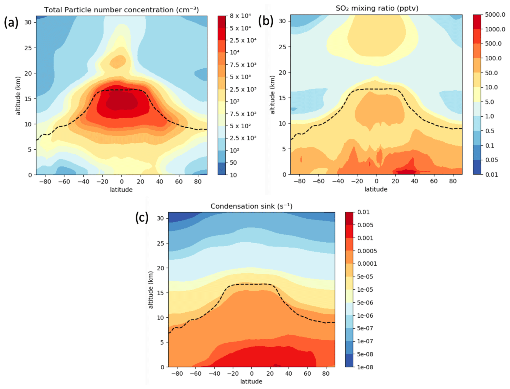
Figure 2Global longitudinal mean vertical profile of the simulated (a) total particle number concentration (NTotal), (b) SO2 mixing ratio and (c) condensation sink from the default version of our model. In this figure, we show altitudes up to 30 km, and our model top is 85 km, but our analysis focuses on the troposphere. The black dashed line represents the tropopause height.
To compare the model with ATom data, we use high temporal resolution 4D model output data along the flight track. The default version of the model shows substantial biases when compared to observations (Appendix Figs. A1, A2 and A3). On investigating these biases, we discovered a bug in the subroutine in which the tendency in H2SO4 concentration in the chemistry scheme was calculated. The chemistry and aerosol processes in the model are handled using the operator-splitting technique, where the usual timestep for chemical reactions is 1 h and the algorithm that handles the chemistry introduces sub-steps where necessary. Microphysical processes (nucleation, condensation and coagulation) are treated on a separate 4 min-long sub-timestep within the 1 h chemistry timestep. The H2SO4 concentration is updated on every microphysics timestep, and this was incorrectly implemented: the production of sulfuric acid from SO2 on the microphysics timestep was missing and the sulfuric acid was being produced only at the beginning of every chemistry timestep. This resulted in an excess H2SO4 concentration at the beginning of every chemistry timestep but no production of H2SO4 later in the timestep. Nucleation is a very non-linear process, and so the high initial H2SO4 concentration resulted in an excessive number of small particles being produced via nucleation. We resolved this bug and used this corrected version, which we refer to as the “baseline” version, as the starting point for our sensitivity analysis in Sect. 6. The released version of UKESM, which we started with, does not contain the bug fix and was used in CMIP6 experiments (Eyring et al., 2016). In this study we refer to this version of the model as the “default” version. Figures 3, 4 and 5 focus exclusively on how the baseline version of the model performs against observations, and a comparison of how the default and baseline versions perform against observations is shown in Appendix Figs. A1, A2 and A3.
The SO2 instrument was only flown on the ATom4 campaign, in spring 2018, while the vertical profiles of NTotal and condensation sink are produced using all of the ATom campaigns, in all four seasons. However, we compare like with like, in that, for example, SO2 observations in spring are compared only with SO2 model data at 3-hourly time resolution in spring. We perform our analysis using the available data; however, our analysis could benefit from more SO2 data. We can also see that the vertical profiles of NTotal and condensation sink for just ATom4 (Appendix Fig. A4) show similar biases to Figs. 3 and 5, which have data from all the ATom campaigns aggregated together.
Figure 3 compares the simulated and measured vertical profile of NTotal and the model–measurement normalised mean bias factor (NMBF) (defined in Eq. 1) (Yu et al., 2006) for the baseline simulation. The global data are divided into three regions: the tropics (25∘ N–25∘ S), mid latitudes (25–60∘ N, 25–60∘ S) and high latitudes (60–90∘ N, 60–90∘ S). The baseline version of UKESM is shown in green and the ATom measurements in black. The magnitude of the model bias is quantified by the value , which is the factor by which the model overestimates or underestimates the observations.
where M indicates the model and O is the observation. A positive NMBF indicates that the model prediction is higher than the measurements and a negative value indicates that the model is lower than the measurements.
The default model substantially overpredicts NTotal (Fig. A1) in the upper troposphere (> 8 km), with a factor of 10–15 overestimate at an altitude of 12 km in the tropics. In the lower free troposphere (between 1 and 3 km) and boundary layer (< 1 km), the model agrees well (NMBF ∼ 0) with observations in the tropics. However, the model underestimates the observations by a factor of 3 in the mid and high latitudes. The baseline (bug-fixed) version of the model shows biases a factor 5–10 lower in the upper troposphere than the default version, for the reasons explained above.
Figure 4 shows the vertical profile of the SO2 mixing ratio in the model. The baseline model is positively biased by approximately a factor 2–6 in the boundary layer regions of the tropics and mid latitudes. In the tropical upper troposphere, the model overpredicts SO2 by up to a factor 2–6, while the biases in the upper-tropospheric mid and high latitudes are negligible. We speculate that the small differences in biases we see between the baseline and default version (Fig. A2) are due to cloud adjustments, which can affect the SO2 concentration and condensation sink. Adjustments arise because changes in NTotal can affect cloud drop concentration and liquid water path and can therefore change the SO2 lost in aqueous chemical processing in clouds.
Figure 5 shows the vertical profile of the condensation sink in the atmosphere. The condensation sink simulated by the baseline version of the model shows positive and negative biases within a factor of 2 of the observations. Larger particles in the atmosphere contribute to the condensation sink, and a higher concentration of these large particles would result in more available surface area for condensable vapours to condense. The bias when comparing the model to observations can be explained by uncertainties in primary aerosol/gas emissions or other atmospheric processes. From the vertical profile it appears that the model either transports larger aerosol particles to the free troposphere or removes too little in precipitation.
To explore any longitudinal differences, we also plotted the observations and model data in the Pacific and Atlantic oceans to briefly explore whether the model shows differing trends in these regions (Appendix Fig. A5). From the figure we can see that the model shows biases of similar magnitude in the Pacific and Atlantic when compared to observations. The model shows biases of up to 10, 5 and 2 for the NTotal, SO2 and condensation sink respectively in the Pacific and Atlantic. We also note that we have lumped Northern Hemisphere and Southern Hemisphere data for the mid and high latitudes. The magnitudes of NTotal, SO2 and condensation sink are different in both hemispheres, and we illustrate that in Appendix Fig. A6. The vertical profiles of all three variables show similar biases in both the northern and southern mid latitudes. In the high latitudes we see more substantial interhemispheric differences. The most notable are that (a) NTotal shows a factor of 5 underprediction in the northern high-latitude boundary layer, with the southern high-latitude boundary layer showing good agreement with observations, and that (b) the model predicts a less than 1 pptv SO2 mixing ratio in the southern high latitudes, with observation showing a mixing ratio of ∼ 10 ppt. We explore ways to reduce these biases in Sects. 6 and 7.
From Figs. 3, 4 and 5, an immediate result of the baseline model evaluation is that the too-high particle number concentration in the free and upper troposphere at tropical and mid latitudes is qualitatively consistent with too-high SO2 mixing ratios but inconsistent with the too-high condensation sink. The possible reasons for the biases in NTotal, SO2 and condensation sink are explored later in Sect. 5.
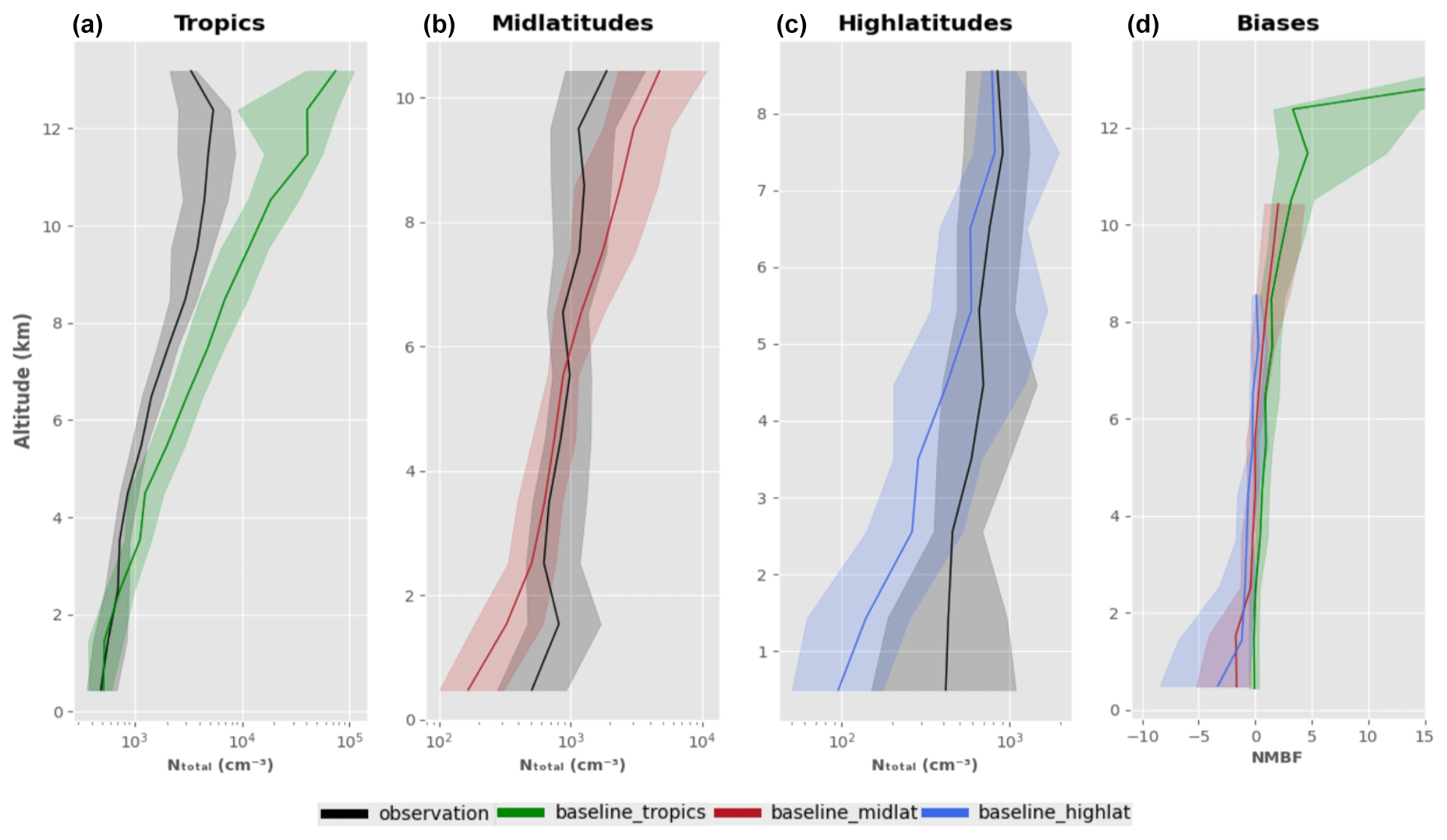
Figure 3The first three columns show the vertical profile of the total particle number concentration (at standard temperature and pressure – STP) as observed (ATom1–4) and in the simulated data from the baseline (bug-fixed) configuration of UKESM in the tropics (25∘ N–25∘ S), mid latitudes (25–60∘ N and 25–60∘ S) and high latitudes (60–90∘ N and 60–90∘ S). The fourth column shows the NMBF of the baseline simulation in the tropics, mid latitudes and high latitudes. The bold line represents the median and the shaded region represents the corresponding interquartile range (25th and 75th percentiles) in a 1 km altitude bin.

Figure 4The first three columns show the vertical profile of the SO2 (at STP) as observed (ATom4, April–May 2018) and the simulated data from the baseline (bug-fixed) configuration of UKESM in the tropics (25∘ N–25∘ S), mid latitudes (25–60∘ N and 25–60∘ S) and high latitudes (60–90∘ N and 60–90∘ S). The fourth column shows the NMBF of the baseline simulation in the tropics, mid latitudes and high latitudes. The bold line represents the median and the shaded region represents the corresponding interquartile range (25th and 75th percentiles) in a 1 km altitude bin.
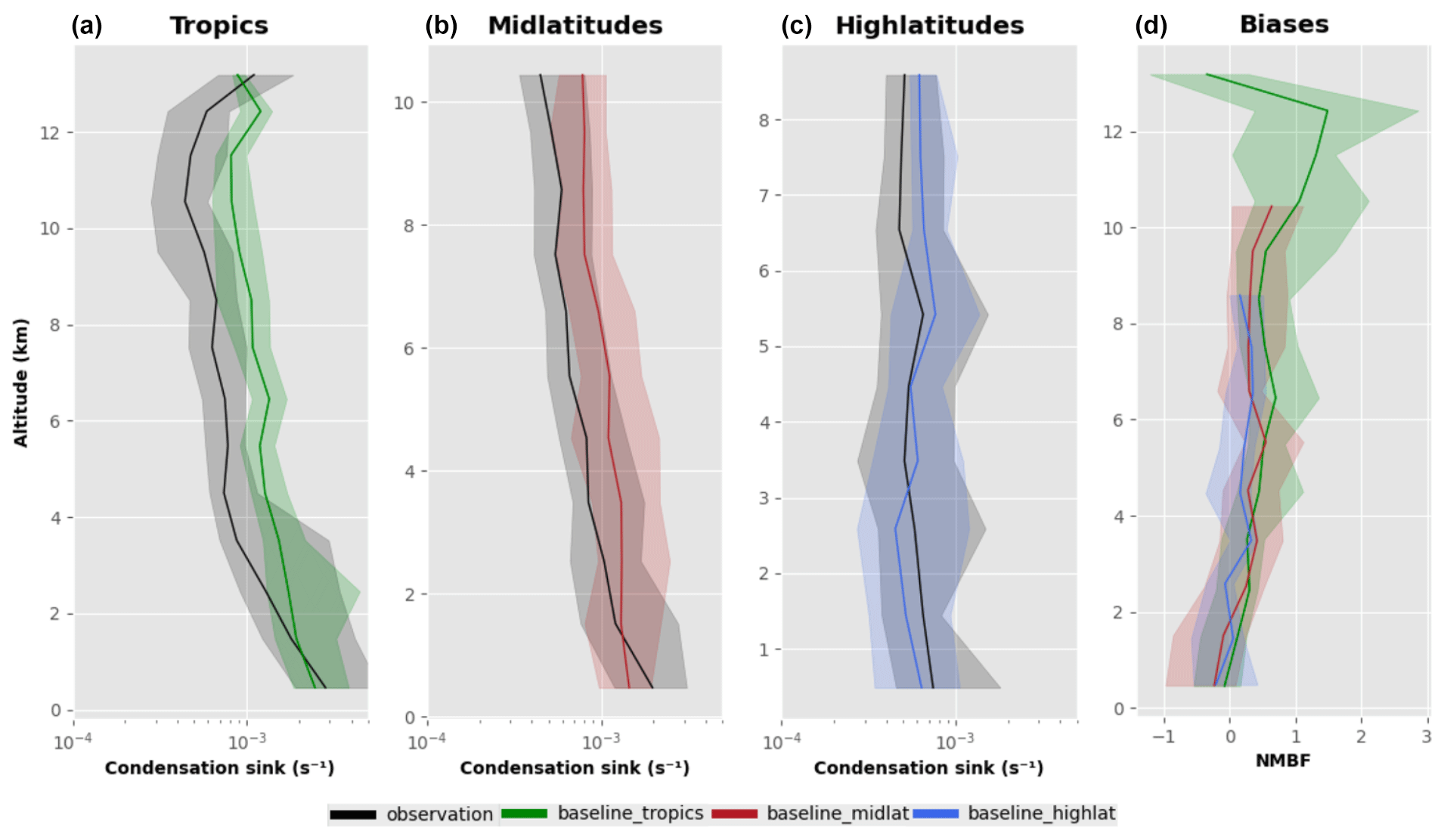
Figure 5The first three columns show the vertical profile of the condensation sink (at STP) as observed (ATom1–4) and in the simulated data from the baseline (bug-fixed) configuration of UKESM in the tropics (25∘ N–25∘ S), mid latitudes (25–60∘ N and 25–60∘ S) and high latitudes (60–90∘ N and 60–90∘ S). The fourth column shows the NMBF of the baseline simulation in the tropics, mid latitudes and high latitudes. The bold line represents the median and the shaded region represents the corresponding interquartile range (25th and 75th percentiles) in a 1 km altitude bin.
To investigate the potential causes of the model biases, we have identified several atmospheric processes that are expected to influence the vertical profile of the NTotal, SO2 and condensation sink. The model simulations that we performed include a combination of direct perturbations to atmospheric processes and changes in model microphysics. The perturbations were applied globally, and we analyse model performance at different regions in the troposphere. A more complete method of sensitivity analysis is to consider the joint effect of a combination of parameters on model performance, which has been done in the past with perturbed parameter ensemble studies (Lee et al., 2013; Regayre et al., 2018). The one-at-a time sensitivity tests that we carry out here help to determine which processes have the largest effect on model biases, and this information can be used in ensemble studies in the future. The atmospheric processes which we have selected for this study along with the motivation for why we picked them are described from Sect. 5.1 to 5.5 and also summarised in Table 1. A more detailed analysis of the effect of these model simulations on model biases is described in Sect. 6, and a three-way comparison of NTotal, SO2 and condensation sink biases is explored in Sect. 7.
Table 1Overview of the atmospheric processes that we have chosen for one-at-a-time sensitivity tests and the magnitude of the perturbation/scaling applied.
5.1 Nucleation rate and nucleation-mode microphysics
Binary homogeneous nucleation. UKESM uses a binary neutral homogeneous H2SO4–H2O nucleation scheme (Vehkamäki et al., 2002) throughout the atmosphere. The upper-tropospheric positive biases in NTotal which we see from Fig. 3 could be because of a high nucleation rate. Therefore, we perform simulations where we reduce the nucleation rate by factors of 10 and 100 to assess its influence on the large bias in upper-tropospheric particle number concentration. These perturbations to the nucleation rate could indirectly compensate for the biases in the production rate of H2SO4 from SO2 (which can affect the concentration of sulfuric acid in the atmosphere, which affects new particle formation). It should be noted that the H2SO4–H2O nucleation scheme (Vehkamäki et al., 2002) is an old scheme and the parameterised nucleation rates are valid only for a limited temperature range (230–305 K). A new nucleation scheme (Määttänen et al., 2018) for the H2SO4–H2O system extended the validity range to lower temperatures and a wider range of environmental conditions. Global particle number concentrations for both schemes were compared in that study (Määttänen et al., 2018), and the vertical profile of particle number concentration was found to be slightly higher (by ∼ 100 particles cm−3) at lower altitude (between 300 and 800 hPa), with particle number concentrations in the upper troposphere (> 300 hPa) being almost identical. This addresses the uncertainty associated with the Vehkamaki nucleation scheme for the H2SO4–H2O system at low temperatures in the upper troposphere. However, this perturbation is not well-motivated by available nucleation parameterisations but is intended only as a candidate for crude tuning to compensate for model biases.
Boundary layer nucleation. We incorporated a boundary layer nucleation (BLN) scheme (Metzger et al., 2010) to account for a source of new particles in the boundary layer to address the model's boundary layer negative bias (Fig. 5). Most of our measurements are over the remote ocean, and the scheme we use is dependent on oxidation products from organics which, in our model, originate only from terrestrial vegetation. However, these organic vapours or the nucleated particles are transported to the remote ocean and thereby affect the vertical profile. The condensation sink is also affected by BLN since the new particles that are formed can grow to larger particles by condensation of sulfuric acid and volatile organic compounds onto their surface (Pierce et al., 2012). We perform one model simulation with boundary layer nucleation included and then one where the boundary layer nucleation rate is reduced by a factor of 10. All of the oxidation products of volatile organic compounds (VOCs) are treated similarly in the model and have been lumped into a tracer called “Sec_org”. This could lead to biases in the BLN rate and condensational particle growth rate since in reality the oxidation products of VOCs have different volatilities which can nucleate and condense at different rates. Reducing this nucleation rate by a factor of 10 (Regayre et al., 2018; Yoshioka et al., 2019) was found to match better with observations.
New particle growth. We improved the handling of the growth of newly formed clusters in the model because the initial stage of particle growth up to about 3 nm diameter is crucial to global CCN concentrations (Gordon et al., 2017; Tröstl et al., 2016) and can affect the vertical profile of particle number concentration. Measurement of particle growth rate at diameters smaller than 3 nm is difficult for most atmospheric instrumentation. This growth of small particles is determined by competing processes where particles grow by condensation of vapour onto the particle surface and are lost by coagulation with larger pre-existing particles (Pierce and Adams, 2007). Particle growth is simulated explicitly for particle sizes larger than 3 nm. However, for the sub-3 nm size range, the growth is represented implicitly by defining an effective rate of production of particles at 3 nm (accounting for competing growth and loss processes). This rate is calculated using a parametrisation (Kerminen and Kulmala, 2002):
where J3 nm and refer to the particle production rate at 3 nm and the critical size (dc) respectively, CS (dc) is the coagulation sink for particles of diameter dc onto pre-existing aerosol and GR is the growth rate of the particles. The coagulation sink for a particle of diameter dp is CS, where K(dpdj) is the coagulation coefficient for particles of diameter dp coagulating onto particles of diameter dj. An assumption made to derive Eq. (2) was that the coagulation coefficient for particles was proportional to the inverse of the square of the particle diameter (). This is not always a sufficiently good approximation, and the power dependency of the coagulation coefficient can vary depending on the ambient particle size distribution which varies from one location on the planet to another (Kürten et al., 2015). For example, observations at Hyytiala in the Finnish boreal forest (Dal Maso et al., 2005) reveal that the power law dependency of the coagulation sink with particle diameter is not −2: it was in a range between −1.5 and −1.75. In a previous study (Lehtinen et al., 2007) a new analytical expression for J3 nm was derived as shown in Eq. (3).
where and .
We have incorporated this new expression into the model, and we show (Sect. 6) that this affects the concentration of smaller particles in the atmosphere by more correctly accounting for their losses due to coagulation.
Coagulation sink. The GLOMAP coagulation scheme (Jacobson et al., 1994) includes both inter-modal (collision between particles that belong to different modes) and intra-modal (collision between particles in the same mode) coagulation. The estimation of the coagulation kernel has uncertainties in the effect of Van der Waals forces and charge on the particles (Nadykto and Yu, 2003). In this study we are focused only on the overall uncertainty of atmospheric processes, so we perturbed the model by scaling up the whole coagulation kernel by a factor of 5 to observe its impact on the model–observation comparison.
Condensation sink. The two condensable species present in the model are H2SO4 (formed from the oxidation of SO2) and Sec_org (formed from the oxidation of monoterpenes). The condensation sink refers to the rate at which these condensable gases condense onto aerosol particles in the atmosphere. It is equal to 2πD∑jβjdjNj, where D is the diffusion coefficient, βj is the transition regime correction factor (Fuchs and Sutugin, 1971), dj is the particle diameter and Nj is the particle number concentration for the jth aerosol mode. It is conceivable that the presence of too much sulfuric acid in the atmosphere results in the formation of excess new particles, which could explain the bias in NTotal. Therefore, having a stronger condensation sink could help reduce the bias. The model also handles the condensation of H2SO4 and Sec_org differently in that the sulfuric acid concentration is updated every microphysics timestep (4 min), while the Sec_org concentration is updated only on every chemistry timestep (1 h). Since condensation in the atmosphere can happen on very short timescales, the Sec_org concentration may need to be updated at the end of every microphysics timestep as well. We perform model runs after incorporating this change into the frequency at which Sec_org is updated and also perform simulations where we manually increase the condensation sink by factors of 5 and 10 to see how sensitive the vertical profiles are to this perturbation (the condensation sink can also be indirectly affected by perturbations to other atmospheric processes). The motivation for increasing the condensation sink by large factors was to test the magnitude of the condensation sink required to reduce the large biases in NTotal. We only perturb the condensation sink directly and not the SO2 or particle number concentration, because perturbing the condensation sink is technically more straightforward.
5.2 DMS and primary marine organic emissions
There is a significant uncertainty in gas-phase DMS emission from the ocean, because the DMS emission fields are derived from a small set of ocean cruise measurements. Interpolation of this small dataset (Kettle and Andreae, 2000; Lana et al., 2011) is used to obtain a global DMS emission field which is used by global models. This results in a large uncertainty range in the DMS annual budget that lies between 17.6 and 34.4 Tg[S] (Lana et al., 2011). From past studies (McCoy et al., 2015; O'Dowd et al., 2004) we know that over marine regions, gas-phase volatile organic compounds emitted from the ocean surface layer are a source of organic-enriched sea-spray aerosol. We also note that the DMS oxidation chemistry is also quite uncertain (Hoffmann et al., 2016; Veres et al., 2020), and this can lead to biases as well. Our default model version included an emission parametrisation with the DMS field scaled up by a factor of 1.7 to account for neglecting primary organic aerosol emissions in the model (Mulcahy et al., 2018). This simplified approach may not be realistic because scaling up DMS emissions will result in a larger production of SO2 and H2SO4 via DMS and SO2 oxidation. Since our goal is to reduce biases in SO2 and particle number, we ran a simulation without the scale factor of 1.7. More recent versions of the model also include an emission parametrisation to estimate the primary marine organic aerosol flux, which is significantly correlated with the chlorophyll concentration (Gantt et al., 2012). Without removing the scale factor of DMS, we tested the sensitivity of aerosol number concentration to this parametrisation by running model simulations with the primary marine organic emissions switched on and also running simulations in which the emissions are scaled up by a factor of 5.
5.3 Cloud pH
Cloud droplet pH is an important parameter in the model because the aqueous-phase oxidation of SO2 by O3 (to form sulfate) (Kreidenweis et al., 2003) is very sensitive to the pH of the cloud droplet. It is assumed in the model that this reaction occurs in all clouds, but the model only tracks the sulfate produced in shallow clouds and not in deep convective clouds, since most of the sulfate formed would be scavenged from the atmosphere by precipitation in convective clouds but not in non-precipitating or lightly precipitating shallow clouds. The rate of this reaction increases by a factor of 105 for a pH change from 3 to 6 (Seinfeld and Pandis, 2016). Droplet pH is important because the consumption of SO2 in a cloud droplet affects the mixing ratio of gas-phase SO2 available in the atmosphere, thereby reducing the gas-phase concentration of H2SO4 (which can form particles). The cloud pH depends on the thermodynamic and kinetic processes in a changing cloud droplet distribution, which are not explicitly simulated in our model; instead a constant cloud pH of 5 is assumed. This assumption could lead to significant errors in regions of the planet where the pH is higher or lower than 5, owing to the regional variability in the amount of acidic and basic material present in the particles. Since we overestimate SO2 compared to ATom observations, we performed perturbations by increasing the pH to 6 and 7 so as to lower the SO2 and NTotal bias. This parameter has also been identified in previous studies as one of the most important parameters for global CCN uncertainty (Lee et al., 2013).
5.4 Scavenging of aerosol particles and gases
The removal of aerosol particles and gases in convective clouds is an important atmospheric process that can control the vertical profiles of NTotal, SO2 and condensation sink. Convection in the model is represented using a mass flux scheme (Gregory and Rowntree, 1990) which is responsible for the vertical transport of aerosol and gases. Understanding the effect of the removal mechanism for aerosol particles and gases during their vertical transport is crucial in quantifying their vertical distribution. In the model, aerosol particles are scavenged using a convective plume-scavenging scheme (Kipling et al., 2013), where scavenging coefficients for aerosol particles are assigned for each mode (denoted by the parameter “rscav”). This convective plume-scavenging scheme addresses, albeit crudely, biases that resulted from operator splitting between scavenging and convective transport and simulation of activation above cloud base, which were subsequently highlighted in other models (Yu et al., 2019). As a plume rises through the atmosphere, the change in aerosol number and mass mixing ratios is dependent on the precipitation rate, convective updraught mass flux, mass mixing ratio of ice and liquid water, and the scavenging coefficients (“rscav”) assigned to each mode. The nucleation mode is not scavenged and is assigned a scavenging coefficient of 0; the Aitken, accumulation and coarse modes are assigned scavenging coefficients of 0.5, 1 and 1 respectively. We assess the sensitivity of the model–observation comparison to perturbations in these values. These scavenging coefficients used are consistent with convective cloud models which show that the aerosol in-cloud scavenging is close to the water-scavenging efficiency (less than 1) (Flossmann and Wobrock, 2010).
We also scale up the convective rain-scavenging rate for all gases (denoted by the parameter “csca”) by factors of 10 and 20. These have higher uncertainty than aerosol-scavenging coefficients because gas uptake into droplets and subsequent removal depends on gas solubility, temperature, ice formation (and gas retention during freezing), and aqueous-phase chemistry (Yin et al., 2002).
5.5 Cloud erosion rate
The cloud erosion rate is an important tuning parameter (represented by UKESM parameter “dbsdtbs”) (Yoshioka et al., 2019) for the prognostic cloud fraction and prognostic condensate scheme (PC2) used in the model (Wilson et al., 2008). This parameter determines the rate at which unresolved subgrid motions mix the clear and cloudy air, thereby removing liquid condensate, and it changes the cloud liquid fraction for shallow clouds. Changing this parameter should have an effect on SO2 lifetime as a result of its uptake into cloud droplets. Its effect on the fraction of cloud in each grid box will also change the amount of shortwave radiation received by the Earth's surface, which in turn can have feedback effects on aerosol processes. This parameter is usually tuned so that the outgoing shortwave radiation the model predicts matches observations. The default value of “dbsdtbs” in the model is . We perform two perturbation simulations with this value set to 0 and another with a value of 10−3.
The goal of the model one-at-a-time sensitivity tests is to understand the causes of biases in the model. Since we are interested in reducing the absolute magnitude of the biases, we use the normalised mean absolute error factor (NMAEF) (Yu et al., 2006) defined in Eq. (4) instead of NMBF to characterise the bias. This new equation allows us to calculate the percentage change in model performance as the relative change in NMAEF of a model experiment with respect to the baseline version of UKESM as shown in Eq. (5).
where Mi represents model data, Oi represents observations, represents the model mean and represents the mean of the observations.
The percentage change is zero when the sensitivity test has no effect on mean model bias, positive when there is an reduction in bias, and negative when the bias increases. A model that is in agreement with observations will have an NMAEF of zero and a percentage improvement of 100 %. Different simulations have varying effects on the vertical profiles at different altitudes in the troposphere, and we have therefore split our analysis to study model performance with altitude. The real boundary layer height varies with latitude, but for the purposes of this study we assume it is 1 km everywhere. Our results are similar for the boundary layer and lower troposphere, suggesting that our analysis is not sensitive to this assumed boundary layer height. In Sect. 6.1 we look closely at the model's performance in the boundary layer (which we define here as altitudes below 1 km) and lower troposphere (1 km < altitude < 4 km), and in Sect. 6.2 we study the mid (4 km < altitude < 8 km) and upper troposphere (> 8 km).
6.1 Boundary layer and lower troposphere
The performance for the different perturbation simulations in the boundary layer (altitude < 1 km) can be assessed from Fig. 6. The NMAEF values for the simulations in the boundary layer are provided in Table 2a. The percentage change in the bias of NTotal, SO2 mixing ratio, and condensation sink from each of these perturbation simulations is calculated relative to the baseline version of UKESM and is represented by bar plots.
Firstly, we look at the model performance with respect to NTotal in the altitude range 0–1 km, where the model is biased low (Fig. 6a). The baseline version of the model produces boundary layer NTotal values that are negatively biased (NMAEF = 2.21). To reduce the bias in particle number concentration near the surface, the model perturbation simulations (denoted as “BL_nuc” and “BL_nuc/10”) that include a boundary layer nucleation mechanism show the best improvement in performance. “BL_nuc” refers to the simulation that includes the Metzger boundary layer nucleation mechanism (Metzger et al., 2010), and “BL_nuc/10” refers to a simulation with the same nucleation mechanism but with the nucleation rate reduced by a factor of 10. Including this nucleation mechanism substantially improves model performance by 63 % (NMAEF = 0.78) for “BL_nuc” and 68 % (NMAEF = 0.72) for “BL_nuc/10”. This is an indication that the negative model bias in the boundary layer (Fig. 3) could be explained by a missing boundary layer nucleation mechanism in the model, even though this mechanism depends on terrestrial emissions of short-lived organic compounds (typically not found in large concentrations over marine regions). A nucleation mechanism other than the Metzger mechanism (Metzger et al., 2010), which could be a scheme controlled by chemical species found in the marine boundary layer like methane sulfonic acid (MSA) (Pham et al., 2005), iodine (Cuevas et al., 2018) or ammonia (Dunne et al., 2016), could help reduce model biases even more but is not the focus of this work. All the other perturbation simulations either have no significant effect or decrease NTotal model performance in the boundary layer. The perturbation simulations that stand out as performing the poorest in the boundary layer are when we increase the pH (denoted by “pH = 6”, NMAEF = 2.75, and “pH = 7”, NMAEF = 2.94), condensation sink (denoted by “condsink*5”, NMAEF = 2.58, and “condsink*10”, NMAEF = 2.89) and scavenging of SO2 (“csca*10”, NMAEF = 2.55, and “csca*20”, NMAEF = 2.61). These perturbations show (Fig. 6a) an approximate decrease of 25 % in NTotal model performance.
Secondly, we look at the parameters that significantly improve the ability of the model to reproduce SO2 mixing ratios in the boundary layer (Fig. 6b), where the model is biased high (NMAEF = 2.09). Figure 6b shows that perturbations to cloud pH, DMS emissions (denoted by “seadms = 1.0”), convective rain-scavenging rate (denoted by “csca*10” and “csca*20”) and the cloud erosion rate (denoted by “dbsdtbs=0”) all improve model performance. The DMS emission perturbation, where we removed the artificial scaling factor of 1.7 that was used to compensate for the lack of primary marine organics, was also found to improve the model performance by 36 % (NMAEF = 1.34). Increases in cloud pH from the default value of 5 to 6 or 7 (denoted in the figure as “pH = 6” and “pH = 7”) improve the model by 34 % (NMAEF = 1.39) and 48 % (NMAEF = 1.09) respectively. In the atmosphere, a lower cloud pH is typically associated with polluted environments where particles are sulfate-rich, and higher cloud pH is associated with marine regions where particles are larger and contain carbonates from sea spray (Gurciullo and Pandis, 1997). Therefore, perturbations to cloud pH by increasing it to 6 or 7 are plausible explanations for the improved model skill since the observations are primarily over the remote ocean. Increasing the pH increases the rate of the reaction in a cloud droplet, thereby resulting in a larger consumption of aqueous SO2. This drives more SO2 from the gas phase to the aqueous phase, thereby reducing the gas-phase SO2 model bias. Increasing the pH can also compensate for the oxidation of SO2 with O3 on sea salt particles, which is shown to be a significant atmospheric process in marine regions (Korhonen et al., 2008). Furthermore, when the cloud erosion rate was set to zero (denoted by “dbsdtbs_0”), it resulted in a model improvement of 25 % (NMAEF = 1.56). A high value for dbsdtbs will cause more mixing of clear and dry air into clouds, thereby reducing the cloud liquid water content, cloud amount, and autoconversion of cloud droplets to raindrops. A low value of this parameter results in an increased lifetime for aerosol and precursor gases like SO2.
Thirdly, we look at the parameters that most affect the model performance with respect to the prediction of the condensation sink (Fig. 6c). The condensation sink in the boundary layer for the baseline version of the model has an NMAEF of 0.82. Simulations where we perturbed the boundary layer nucleation rate (“BL_nuc” and “BL_nuc/10”) and the primary marine organic emissions (“primmoc*5”) showed 15 % (NMAEF = 0.69), 10 % (NMAEF = 0.73) and 25 % (NMAEF = 0.61) improvements in bias. This could be because the boundary layer is lacking particles, and including a new source of particles via boundary layer nucleation and emissions reduces the negative bias in the boundary layer (Fig. 6c). The simulations where we increase the condensation sink by factors of 5 and 10 show larger biases (NMAEF = 2.46 and 5.5 respectively). These perturbations are somewhat unrealistic, because the baseline version already agrees well (within a factor of 2) with observations, but they are useful as tests of the sensitivity of new particle formation in the model to the condensation sink.

Figure 6Percentage change in model performance for different perturbation simulations in the boundary layer (altitude < 1 km) with respect to (a) NTotal, (b) SO2, and (c) condensation sink.
The atmospheric processes that improve the skill of the model in the lower troposphere (between 1 and 4 km) (Appendix A, Fig. A7) (NMAEF values are shown in Appendix A, Table A2) are the same as the boundary layer, with very slight differences in the magnitude of the percentage change in model performance.
6.2 Mid and upper troposphere
The model sensitivities in the upper troposphere are shown in Fig. 7. Firstly, we assess NTotal model performance for all the model simulations (Fig. 7a). We observe that perturbations to several atmospheric processes help improve the model performance. Perturbations to the condensation sink, nucleation rate, sub-3 nm growth, DMS emissions, gas-scavenging rate, cloud erosion rate and cloud pH are found to have a significant effect on model performance. The range of parameter sensitivities is more diverse than in the boundary layer, and the magnitudes are larger.
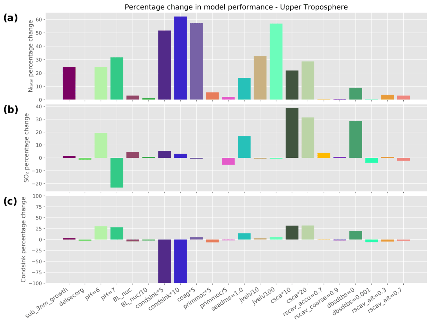
Figure 7Percentage change in model performance for different perturbation simulations in the upper troposphere (> 8 km) with respect to (a) NTotal, (b) SO2, and (c) condensation sink.
First, we look at the model's performance with respect to NTotal. The baseline simulation produces NTotal values that are biased high (NMAEF = 3.25) in the upper troposphere (Table 2b). The most improvement in model performance with respect to NTotal (Fig. 7a) was for the model simulations, where we directly perturbed the condensation sink. These model runs were denoted as “condsink*5” and “condsink*10” and show an improvement in performance by 51 % (NMAEF = 1.57) and 62 % (NMAEF = 1.23) respectively (Table 2b). This improvement in performance is because increasing the condensation sink will increase the rate at which H2SO4 is removed from the atmosphere via condensation onto particles. Therefore, increasing the condensation sink can help reduce the H2SO4 concentration and thus reduce the NTotal bias. However, as noted earlier, directly scaling the condensation sink by factors of 5 and 10 in this way is unrealistic, as the model's condensation sink is within a factor of 2 of observations (Fig. 6)
Perturbations to nucleation rate where we reduced nucleation rate by factors of 10 and 100 (denoted as “Jveh/10” and “Jveh/100”) also improved the model by 32 % (NMAEF = 2.19) and 56 % (NMAEF = 1.4) respectively. This improvement in model performance by reducing nucleation rate is an indication that the sources of the biases in NTotal are mainly from small particles formed via nucleation. Model runs where we increase the convective gas-scavenging rate (denoted as “csca*10” and “csca*20”) by factors of 10 and 20 result in 21 % (NMAEF = 2.54) and 28 % (NMAEF = 2.32) improvements respectively. This scavenging rate simply scavenges the SO2 from the atmosphere at a higher rate, which leaves less SO2 to form H2SO4 via oxidation and therefore decreases NTotal. The cloud pH perturbation simulations show 25 % (NMAEF = 2.45) and 31 % (NMAEF = 2.22) improvements for “pH = 6” and “pH = 7” respectively. Increasing cloud pH would increase the oxidation rate of SO2 by ozone in cloud droplets (to form sulfate), thereby causing a reduction in the concentration of gaseous H2SO4. Incorporating the dependency of the coagulation sink on particle diameter (by using the Lehtinen et al., 2007, parametrisation denoted as “sub_3nm_growth”) reduces the positive bias in the model and improves the model by 24 % (NMAEF = 2.45). This is because in the new expression (Lehtinen et al., 2007) the coagulation sink for sub-3 nm particles is greater than the previous assumption (Kerminen and Kulmula, 2002).
Second, we analyse the model sensitivity and performance with respect to SO2 (Fig. 7b and Table 2). The baseline simulation produces SO2 mixing ratios that are biased high (NMAEF = 1.3). The simulations that have the strongest effect on the biases are the perturbations to the DMS emissions (“seadms = 1.0”), cloud pH (“pH = 6”) and SO2 scavenging rate (“csca*10” and “csca*20”): they improve the model by 17 % (NMAEF = 1.08), 19 % (NMAEF = 1.05), 38 % (NMAEF = 0.80) and 31 % (NMAEF = 0.89) respectively (Table 2). The large SO2 over-prediction by the model in the tropical upper troposphere (NMAEF = 1.3) is corrected by the perturbations where the SO2 in the atmosphere is removed by scavenging (“csca*10” and “csca*20”), by reduction in DMS emissions (“seadms = 1.0”) or by reduction in the SO2 mixing ratio as a result of increasing the cloud droplet pH. However, the simulation with cloud pH set to 7 results in too much SO2 being removed by lower-level clouds, leaving less available SO2 to be convected to the upper troposphere, causing a large negative bias (NMAEF = 1.6).
Third, we look at the model performance with respect to the condensation sink (Fig. 7c), where the model is biased with NMAEF = 0.61. The perturbations cloud pH (“pH = 6” and “pH = 7”), convective gas-scavenging rate (“csca*10” and “csca*20”), cloud erosion rate (“dbsdtbs = 0”) and DMS emissions (“seadms = 1.0”) all improve model performance by 15 %–30 %. Increasing the pH of a cloud drop enhances SO2 aqueous-phase chemistry in low-level clouds to form sulfate, which partitions sulfur to the aqueous phase and increases wet removal, leaving less SO2 to be convected upward to higher altitudes. This also results in a reduction in the concentration of larger particles being transported by convection to higher altitudes, thereby reducing the condensation sink to match better with observations. Similarly, reduction in cloud erosion rate will result in greater uptake of SO2 on cloud droplets to form sulfate, thereby increasing aerosol mass and increasing the amount of scavenged larger particles. The other perturbations, where we indirectly influenced the SO2 mixing ratio in the atmosphere by reducing the DMS emissions and SO2 scavenging, also reduce the positive bias in the model condensation sink by reducing the SO2 available to form sulfate.
The atmospheric processes that are of significance to model performance with respect to NTotal and condensation sink in the mid troposphere are similar to the upper troposphere, with decreases in the magnitude of model performance (Fig. A8) relative to the upper troposphere. This indicates that the atmospheric processes that have been identified are of more importance at higher altitudes. However, the model performance with respect to SO2 in the mid troposphere shows more similarity to the lower troposphere (Fig. A7).
7.1 Effect of perturbations on multiple variables
The main reason for analysing NTotal, SO2 and condensation sink model performance simultaneously is to make sure that performing one-at-a-time sensitivity tests to assess model performance leads to a consistent result. Improving only one of these quantities in comparison with observations can lead to a misleading impression that overall model performance has improved. Analysing NTotal, SO2 and condensation sink simultaneously helps reduce the probability of getting the right answer for the wrong reasons. We find that different atmospheric processes affect the vertical profile of NTotal, SO2 and condensation sink to varying degrees.
Firstly, we analyse the boundary layer (< 1 km) and lower troposphere (1–4 km). In Sect. 6.1 we identified the atmospheric processes that are important for the boundary layer and how they affected model performance with respect to NTotal, SO2 and condensation sink independently. Here we look at which simulations perform best when comparing these variables simultaneously. Table 2 shows the NMAEF in the boundary layer and upper troposphere for all of the simulations. The NMAEF values for the baseline simulation are highlighted in yellow, the green boxes represent NMAEF values for the simulations that have the same or lower biases than the baseline simulation, and the orange boxes represent those simulations that have higher biases than the baseline simulation. The results show that the model simulations where we perturbed the cloud pH, DMS emissions, convective gas-scavenging rate and cloud erosion rate all significantly reduce biases with respect to SO2 but make the model perform worse with respect to NTotal and the condensation sink. In Table 2, the blue dotted boxes highlight the simulations for which the biases with respect to NTotal, SO2 and condensation sink are less than or equal to the baseline simulation. The only model simulation that improved NTotal, SO2 and condensation skill simultaneously was when we included boundary layer nucleation (“BL_nuc” and “BL_nuc/10”). Including a boundary layer nucleation scheme adds a new source of particles which helps reduce the negative bias the model shows in the boundary layer.
Table 2Normalised mean absolute error factor (NMAEF) with respect to NTotal, SO2 and condensation sink for different model simulations. NMAEF values for the baseline simulation are highlighted in yellow. NMAEF values that are less than or equal to the baseline simulation are highlighted in green. NMAEF values that are greater than the baseline simulation are highlighted in orange. The plus (+) and minus (−) signs next to each NMAEF value indicate whether the bias is positive or negative. The dotted blue box indicates the model simulation for which NMAEF values for NTotal, SO2 and condensation sink are less than the baseline simulation simultaneously: (a) boundary layer (below 1 km) and (b) upper troposphere (> 8 km).

In the upper troposphere (Table 2b), several simulations improve NTotal model performance. The positive model bias in NTotal is significantly reduced by perturbations to the sub-3 nm growth, cloud pH, condensation sink, coagulation sink, primary marine organic emissions, DMS emissions, nucleation rate, and SO2 gas-scavenging rate. Direct perturbations to the condensation sink, although they improve NTotal model skill significantly, worsen the model performance with respect to the condensation sink (NMAEF = 12.1 for the “condsink*10” simulation). Thus, from Table 2b, the blue dotted boxes indicate the simulations for which the model biases for NTotal, SO2 and condensation sink are less than (or equal to) the baseline version of the model simultaneously.
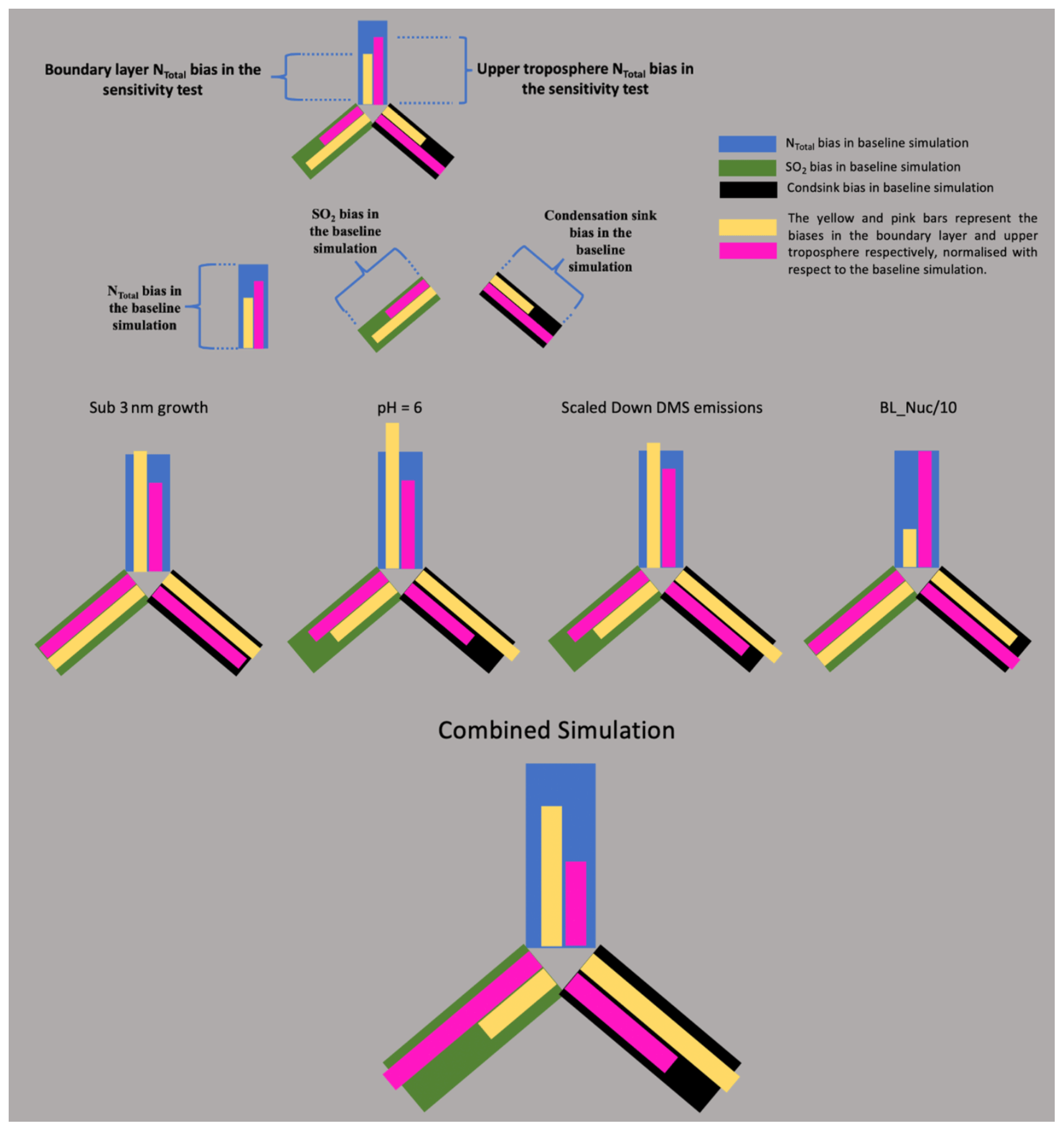
Figure 8Diagram to represent the NTotal, SO2 and condensation sink biases (in the boundary layer and upper troposphere) for the one-at-a-time sensitivity tests: sub-3 nm growth, cloud pH = 6, scaling down DMS emissions, and boundary layer nucleation/10. The blue, green and black legs of the diagram represent the NTotal, SO2 and condensation sink bias respectively. The yellow and pink bars represent the biases in the boundary layer and upper troposphere normalised with respect to the baseline simulation.
We see this simultaneous reduction of biases in the mid (Table A2) and upper troposphere for simulations where we perturbed sub-3 nm growth, cloud pH, DMS emissions, nucleation rate, SO2 gas-scavenging rate and cloud erosion rate. The one main difference between the simulations in the mid and upper troposphere is that the perturbation to cloud pH (pH = 7) improves overall model performance in the mid troposphere but not in the upper troposphere. At pH = 7 the model in the upper troposphere also shows a larger SO2 bias (NMAEF = 1.6) than the baseline (NMAEF = 1.3).
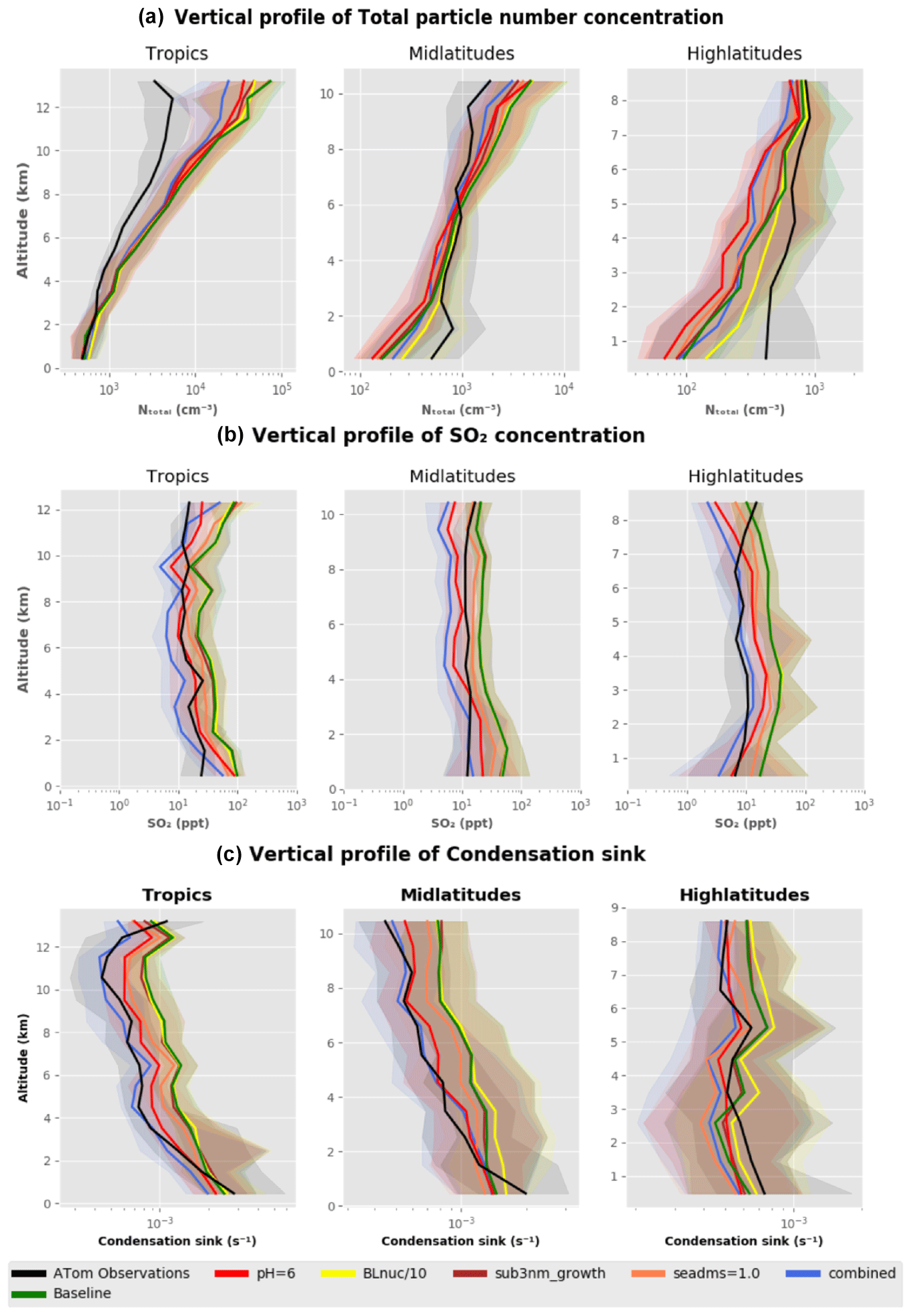
Figure 9The vertical profile of (a) NTotal, (b) SO2 and (c) condensation sink for different model experiments that were found to have the most influence on model performance. The vertical profiles of observation data, the baseline simulation and perturbation simulations of cloud pH, boundary layer nucleation, sub-3 nm growth, scaled-down DMS emissions, and the combined simulation are shown and categorised into three regions of the Earth: the tropics (25∘ N–25∘ S), mid latitudes (25–60∘ N and 25–60∘ S), and high latitudes (60–90∘ N and 60–90∘ S).
We show the combined model bias for a select few sensitivity tests in the boundary layer and upper troposphere using a bar diagram (Fig. 8). In this presentation, the blue, green and black bars represent the normalised NMAEF in NTotal, SO2 and condensation sink for the baseline simulation. The yellow and pink bars represent the corresponding biases in the boundary layer and upper troposphere for any given sensitivity test (normalised with respect to the baseline simulation). If the lengths of the blue, green or black bars are greater than the length of the corresponding yellow and pink bars, then the bias in the sensitivity test is less than the baseline simulation. The vertical profiles for the simulations used in Fig. 8 are shown in Fig. 9. Simulations where we perturbed sub-3 nm growth, pH = 6, DMS scaling, and boundary layer nucleation/10 showed a reduction in biases and in some cases negligibly increased biases. The boundary layer nucleation simulation (BL_nuc/10) reduces biases in the boundary layer NTotal by ∼ 67 % without affecting the upper-tropospheric NTotal bias. This simulation does not have any effect on the SO2 mixing ratio but does reduce the condensation sink bias in the boundary layer by ∼ 11 % and shows a negligible change in bias (∼ 2 %) in the upper troposphere. Changing the pH to 6 causes a slight degradation in the model's NTotal and condensation sink (increase in bias by ∼ 24 % and ∼ 8 %) in the boundary layer and improved the SO2 by 33 %. However, in the upper troposphere perturbations to pH have a positive effect on model performance against observations. The “sub_3nm_growth” simulation improves the upper-tropospheric NTotal bias by ∼ 24 % without significantly affecting other parameters. Removing the scaling factor for DMS emission helps improve the upper-tropospheric NTotal, SO2, and condensation sink bias by 16 %, 17 % and 14 % respectively. It also reduces the boundary layer SO2 bias by 35 % and shows small increases of 6 % and 10 % in the NTotal and condensation sink bias respectively. Thus, we have identified the perturbation simulations, “BL_nuc/10”, “pH = 6”, “Seadms = 1.0” and “sub_3nm_growth”, as the simulations that help reduce model biases in most cases across NTotal, SO2 and condensation in the boundary layer and upper troposphere. These perturbations are well-motivated in that they improve the physical basis of the model and can be looked at more closely when developing future versions of UKESM.
7.2 Effect of combined perturbations on multiple variables
We performed one simulation incorporating the four perturbations (BL_nuc/10, pH = 6, “Seadms = 1.0” and “sub_3nm_growth”) discussed in Sect. 7.1 simultaneously (bottom row in Fig. 8) to assess model performance. For NTotal, the model's boundary layer and upper-tropospheric performance is improved (NMAEF reduced by 24 % and 54 % respectively). The positive SO2 bias improves by 54 % in the boundary layer but showed a slight degradation of 10 % in the upper troposphere. The positive condensation sink bias shows a negligible increase of 4 % in the boundary layer and a 29 % decrease in the upper troposphere. From Fig. 9, the SO2 profile for the combined simulation shows better agreement with observations in the tropics and high latitudes and shows a small negative bias in the mid-latitude free troposphere. The condensation sink profile of the combined simulation does show a much better agreement with the observations in the tropics, mid latitudes and high latitudes. The combined simulation also shows a substantial reduction in the upper-tropospheric NTotal bias in the tropics and mid latitudes, but the large negative bias in the high latitudes remains, and at high altitudes in the high-latitude regions it is exacerbated. In the boundary layer, the combined simulation shows a small improvement in the mid latitudes but otherwise performs similarly to the baseline simulation. The interhemispheric differences in the vertical profile of the combined simulation and baseline simulation are shown in the Appendix (Fig. A9). Overall, the combined simulation performs better than the baseline simulation in both hemispheres, with a couple of notable exceptions. The combined simulation underpredicts observations of NTotal in the southern high-latitude upper troposphere and of SO2 concentration in the northern high-latitude upper troposphere by up to a factor of 2 more than the baseline simulation. We speculate that a marine nucleation mechanism or regional changes in cloud pH that are not simulated in the model currently could be the reason for these interhemispheric biases.
In the tropical free troposphere, the fact that the SO2 and condensation sink for the combined simulation agree very well with observations and NTotal is still overpredicted suggests a missing loss process for nucleation-mode particles in the upper troposphere or a bias in the downward transport of these particles to lower altitudes. The biases in NTotal in the high-latitude and mid-latitude boundary layers for the combined simulation could be because of a missing source of small particles from a marine nucleation mechanism which is not included in the model, for example involving iodine or methane sulfonic acid (Baccarini et al., 2018; Hodshire et al., 2019). Even though simulations with the Metzger boundary layer nucleation scheme (Metzger et al., 2010) helped reduce this bias, this nucleation scheme is primarily dependent on the concentration of organic vapours from terrestrial sources, which are low over marine regions. The biases in the boundary layer high latitudes could also be due to uncertainties associated with the sea-spray parametrisation in the model (Regayre et al., 2020).
To summarise, our new combined simulation performs significantly better than the baseline model we started with for all three variables, NTotal, SO2 and condensation sink. However, we were still unable to reproduce observations of NTotal in the tropical free troposphere, the mid-latitude boundary layer, and the high latitudes with the well-motivated adjustments we applied. Clearly structural errors in the model remain, possibly associated with the way that aerosols and trace gases are incorporated into the convection parametrisation (Prein et al., 2015) or other atmospheric processes: this study motivates future model developments to address the biases and indicates where the developments should be focused.
We have evaluated the vertical profile of NTotal, SO2 and condensation sink from UKESM against ATom aircraft measurements. The model captured the trends in the vertical profiles. Quantitatively, the model reproduced the vertical profile of condensation sink moderately well but shows higher biases in the NTotal and SO2 vertical profile. We performed model simulations to help understand which atmospheric processes influence the model skill and thereby help match the model's prediction of NTotal, SO2, and condensation sink simultaneously with observations. We found that different atmospheric processes have a varying impact on model skill with altitude.
In the boundary layer and lower troposphere, the model showed negative biases in NTotal (up to a factor of 3) and positive biases in SO2 (up to a factor of 6) with moderate positive/negative model biases in the condensation sink (within a factor of 2). We found that simulations with boundary layer nucleation included were the only simulations that reduced the biases in NTotal and condensation sink in the boundary layer simultaneously with negligible changes to the SO2 mixing ratio.
In the middle and upper troposphere, the largest biases were again observed in NTotal (positive biases up to a factor of 15) and SO2 (positive biases up to a factor of 6), with the model's condensation sink showing modest positive/negative biases (within a factor of 2). However, in contrast to lower altitudes, we found that adjustment of several atmospheric processes improved overall model performance. From our one-at-a-time sensitivity tests we found that simulations with perturbations to the sub-3 nm growth, cloud pH, DMS emissions, nucleation rate, gas-scavenging rate and cloud erosion rate all help reduce model biases in NTotal, SO2, and condensation sink simultaneously at higher altitudes.
Simulations where we increased the condensation sink by a factor of 10 or reduced the nucleation rate by a factor of 100 also substantially improved the model's NTotal profile in the tropical upper troposphere. However, while useful to understanding the sensitivity, artificial adjustment of the condensation sink is unrealistic because the model shows only a factor of 2 bias compared to observations. Substantial reduction of the nucleation rate was also explored as this is the main source of particles in the cold upper troposphere. However, the default nucleation rate (Vehkamäki et al., 2002) has been shown to be reasonably accurate or even underestimated for a given sulfuric acid concentration, temperature and humidity (Määttänen et al., 2018). If the effective nucleation rate in the model is indeed too high by a factor of 100, then this may instead suggest a structural deficiency in the way nucleation is implemented in the model, which we discuss below. Any adjustment of the nucleation rate itself is not supported by our current understanding of the rate of nucleation under upper-tropospheric conditions.
Though there are differences in the importance of certain atmospheric processes over others at low and high altitudes, we have identified a few well-motivated changes that help reduce the bias in the boundary layer and upper-tropospheric regions of the tropics, mid latitudes and high latitudes. From our analysis we can suggest the following.
-
Including a boundary layer nucleation scheme helps reduce model biases at lower altitudes without causing large changes in biases in the upper troposphere.
-
Changing the value of cloud pH from 5 to 6 produces a significant improvement in model performance in the mid and upper troposphere. However, this change does result in a slight degradation of the model's NTotal profile at lower altitudes.
-
Improvements to the model's microphysics by updating the parametrisation of nuclei growth (Kerminen and Kulmala, 2002) to include a corrected dependency of coagulation sink on particle diameter (Lehtinen et al., 2007) improves upper-tropospheric model performance without significant degradation of the model at lower altitudes.
-
Removing the scaling factor for DMS emissions also helps reduce the positive biases in SO2 in both the boundary layer and upper troposphere. This simulation does however increase the biases in NTotal and condensation sink in the boundary layer.
We performed a simulation with these four perturbations included simultaneously and found the model's performance in the boundary layer and upper troposphere improved simultaneously. The combined simulation's SO2 and condensation sink profiles agree very well with observations and perform much better than the baseline simulation. However, the NTotal profile for the combined simulation in the tropics and high latitudes, while performing better than the baseline simulation, still has significant biases when compared to observations. The fact that this adjusted simulation reduces the NTotal bias but does not completely eliminate it will help us identify the possible deficiencies of the model in future work. The absence of a scavenging mechanism for nucleation-mode particles (for example on cirrus clouds) or uncertainties in the downward transport of particles could explain the reason for the NTotal positive bias in the upper troposphere–tropics. The negative bias in the boundary layer NTotal could be explained by uncertainties associated with the sea-spray parametrisation or the absence of a nucleation scheme involving gaseous precursors found in the marine environment. Thus, in this work, we have identified several atmospheric processes and parameters in UKESM that are key to the skilful simulation of SO2 mixing ratio, condensation sink and NTotal simultaneously, although we reached a limit in how much the NTotal can be improved upon with the current set of simulations. These perturbations shed light on the influence of different atmospheric processes on aerosol number concentration and motivate further development of parameterisations in the model. Our work will also help inform future perturbed parameter ensemble studies designed to analyse and constrain the effect of a combination of parameters on model skill.
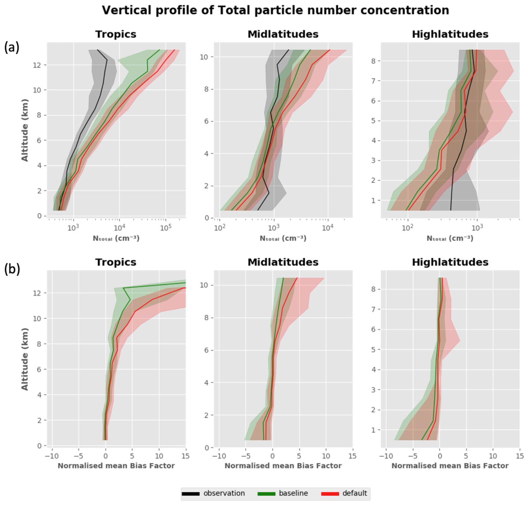
Figure A1(a) The vertical profile of the total particle number concentration (at standard temperature and pressure – STP) as observed (ATom1–4) and in the simulated data from the default and baseline (bug-fixed) configurations of UKESM. (b) The vertical profile of the normalised mean bias factor (NMBF) for the two configurations of the model. The vertical profiles have been provided for the tropics (25∘ N–25∘ S), mid latitudes (25–60∘ N and 25–60∘ S) and high latitudes (60–90∘ N and 60–90∘ S). In both (a) and (b) the bold line represents the median and the shaded region represents the corresponding interquartile range (25th and 75th percentiles) in a 1 km altitude bin.
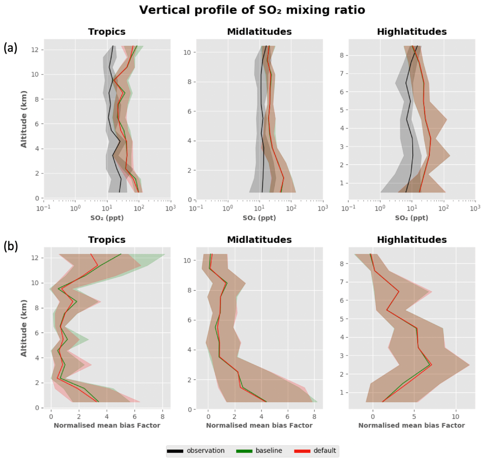
Figure A2(a) The vertical profile of the SO2 mixing ratio as observed (ATom4, April–May 2018) and in the simulated data from the default and baseline configurations of UKESM. (b) The vertical profile of the NMBF for the two configurations of the model. The vertical profiles have been provided for the tropics (25∘ N–25∘ S), mid latitudes (25–60∘ N and 25–60∘ S) and high latitudes (60–90∘ N and 60–90∘ S). In both (a) and (b) the bold line represents the median and the shaded region represents the corresponding interquartile range (25th and 75th percentiles) in a 1 km altitude bin.
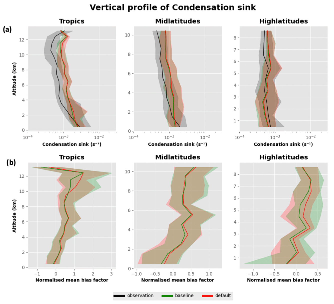
Figure A3(a) The vertical profile of the dry condensation sink in the atmosphere, as observed, and in simulated data from the default and baseline configurations of UKESM. (b) The vertical profile of the NMBF for the two configurations of the model. The vertical profiles have been provided for the tropics (25∘ N–25∘ S), mid latitudes (25–60∘ N and 25∘ S–60∘ S) and high latitudes (60–90∘ N and 60–90∘ S). In both (a) and (b) the bold line represents the median and the shaded region represents the corresponding interquartile range (25th and 75th percentiles) in a 1 km altitude bin.
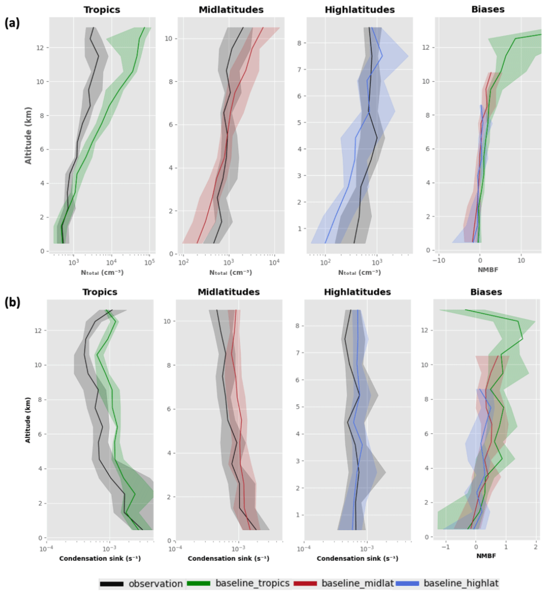
Figure A4Vertical profiles of the baseline model and observation (a) NTotal and (b) condensation sink for only the ATom4 campaign. The first three columns show the vertical profile (at standard temperature and pressure – STP) as observed and in the simulated data from the baseline (bug-fixed) configuration of UKESM in the tropics (25∘ N–25∘ S), mid latitudes (25–60∘ N and 25–60∘ S) and high latitudes (60–90∘ N and 60–90∘ S). The fourth column shows the NMBF of the baseline simulation in the tropics, mid latitudes and high latitudes. The bold line represents the median and the shaded region represents the corresponding interquartile range (25th and 75th percentiles) in a 1 km altitude bin.
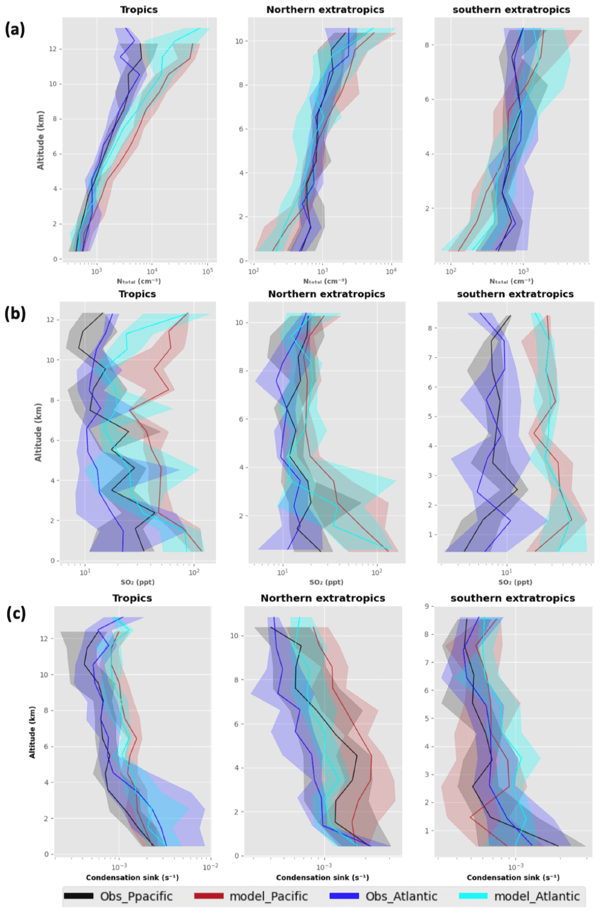
Figure A5The vertical profiles of the ATom and baseline models (tropics, northern extratropics, 25–90∘ N, and southern extratropics, 25–90∘ S) in the Pacific and Atlantic oceans: (a) NTotal, (b) SO2, and (c) condensation sink.

Figure A6(a) The vertical profile of the total particle number concentration, (b) the vertical profile of the SO2 mixing ratio and (c) the vertical profile of the condensation sink. The vertical profiles are provided for the northern and southern mid latitudes (25–60∘ N and 25–60∘ S) as well as the northern and southern high latitudes (60–90∘ N and 60–90∘ S). The bold line represents the median and the shaded region represents the corresponding interquartile range (25th and 75th percentiles) in a 1 km altitude bin.
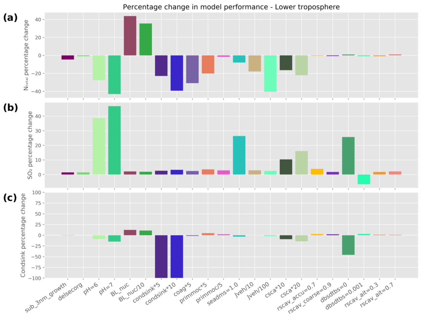
Figure A7Percentage change in model performance for the different perturbation experiments in the lower troposphere (1 km < altitude < 4 km) with respect to (a) NTotal, (b) SO2, and (c) condensation sink.
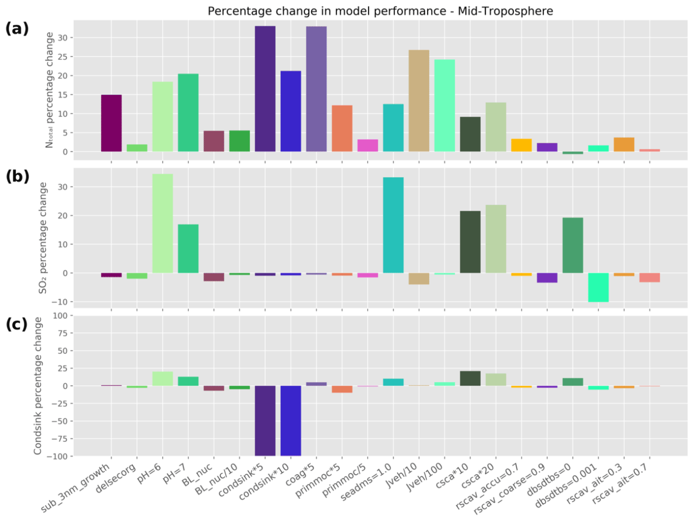
Figure A8Percentage change in model performance for the different perturbation experiments in the mid troposphere (4 km < altitude < 8 km) with respect to (a) NTotal, (b) SO2, and (c) condensation sink.
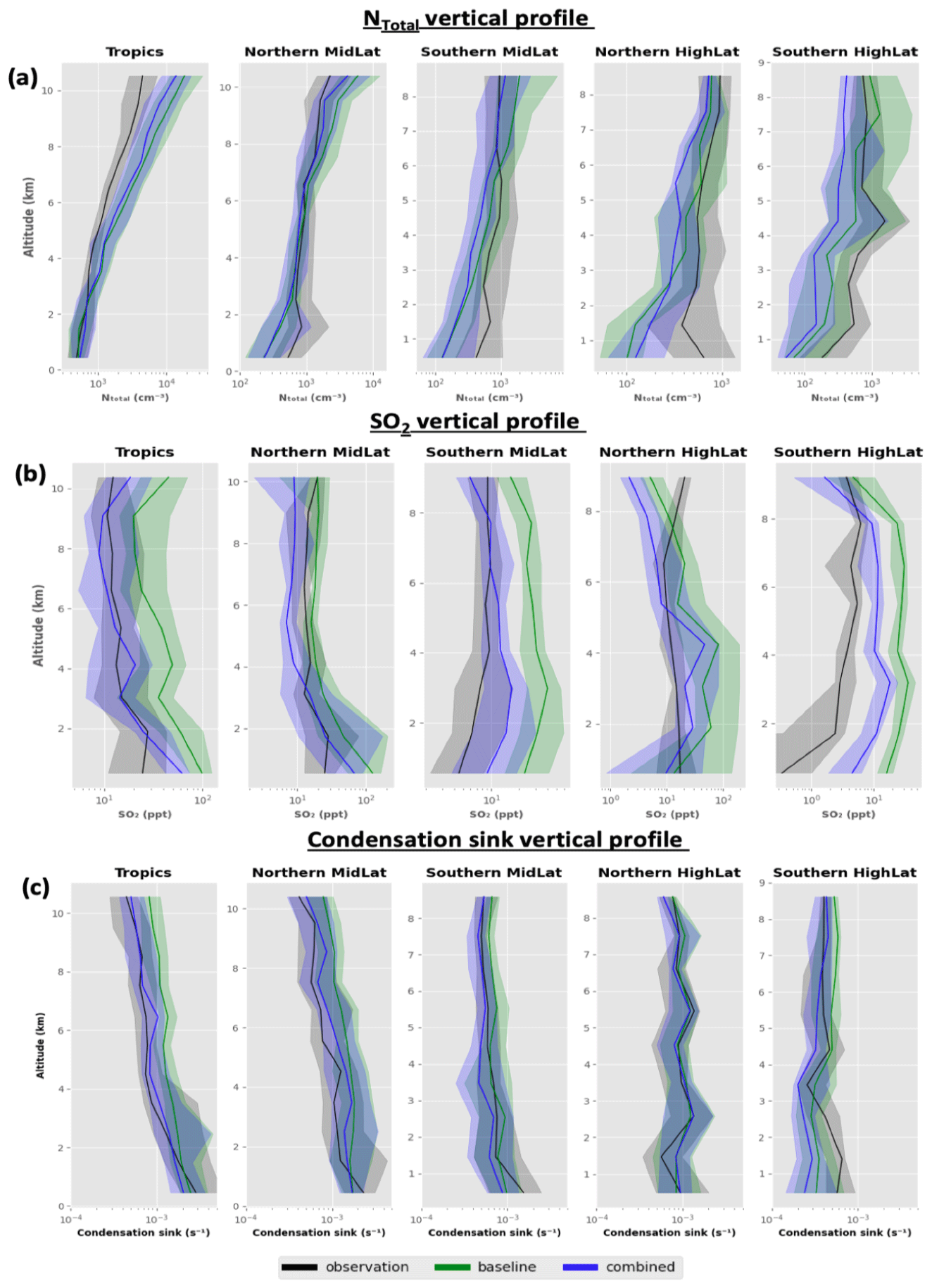
Figure A9The vertical profiles for the baseline simulation and the combined simulation (a) NTotal, (b) SO2, and (c) condensation sink in the tropics (25∘ S–25∘ N), northern mid (25–60∘ N) and high latitudes (60–90∘ N), and southern mid (25–60∘ S) and high latitudes (60–90∘ S).
Table A1The different aerosol size modes in UKESM along with their size ranges, mode standard deviation and aerosol species in each mode. The species are organic matter (OM), sulfate (SO4), BC (black carbon) and sea salt. Dust is treated separately as described in the text.

Table A2Normalised mean absolute error factor (NMAEF) with respect to NTotal, SO2 and condensation sink for different model simulations. NMAEF values for the baseline simulation are highlighted in yellow. NMAEF values that are less than (or equal to) the baseline simulation are highlighted in green. NMAEF values that are greater than the baseline simulation are highlighted in orange. The plus (+) and minus (−) signs next to each NMAEF value indicate whether the bias is positive or negative. The dotted blue box indicates the model simulation for which NMAEF values for NTotal, SO2 and condensation sink are less than (or equal to) the baseline simulation simultaneously: (a) lower troposphere (between 1 and 4 km) and (b) mid troposphere (between 4 and 8 km).
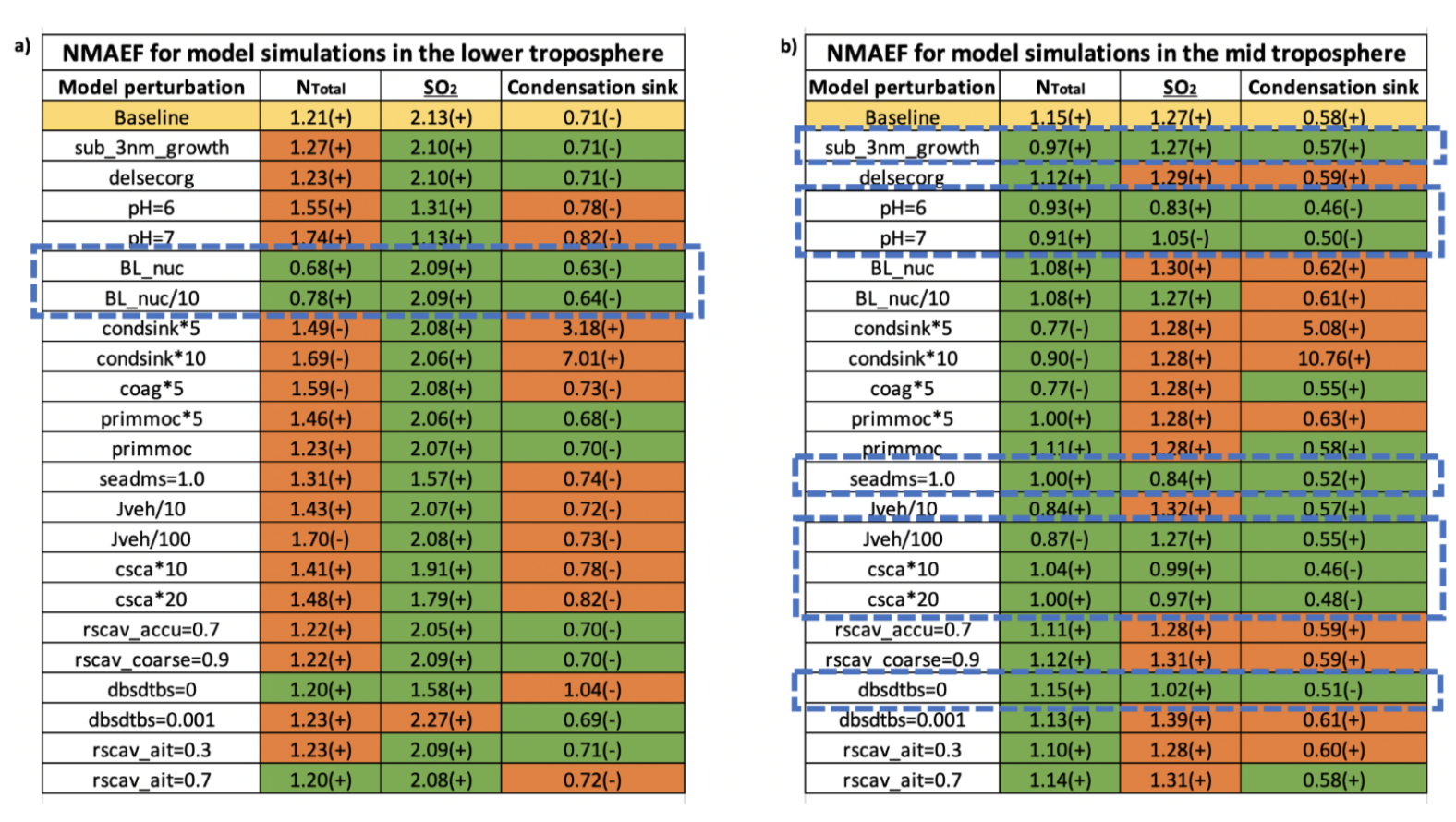
All model and observation data used in this study can be accessed from https://doi.org/10.5281/zenodo.4088640 (Ranjithkumar, 2020). The observations from the ATom campaign can also be obtained from Wofsy et al. (2018).
AnaR, HG and KC designed the idea for this study. AnaR performed all model simulations and analysis with guidance from HG and KC. CW, AK, AndR and CB were responsible for the data from the ATom campaign used in this study. HG and NLA helped identify and resolve the bug in the model code discussed in the article. KP provided scientific guidance and infrastructure support. AnaR wrote the manuscript with help from HG and KC and contributions from all the co-authors.
The authors declare that they have no conflict of interest.
We thank the ATom science team and the NASA DC-8 flight crew for their contributions to the ATom dataset. We are grateful for the use of the MONSooN system, a collaborative facility supplied under the Joint Weather and Climate Research Programme, a strategic partnership between the Met Office and the Natural Environment Research Council. We also thank all the people responsible for the development of UKESM.
This research has been supported by the H2020 Marie Skłodowska-Curie Actions (grant no. 764991, “CLOUDMOTION”).
This paper was edited by Veli-Matti Kerminen and reviewed by two anonymous referees.
Albrecht, B. A.: Aerosols, cloud microphysics, and fractional cloudiness, Science, 245, 1227–1230, https://doi.org/10.1126/science.245.4923.1227, 1989.
Archibald, A. T., O'Connor, F. M., Abraham, N. L., Archer-Nicholls, S., Chipperfield, M. P., Dalvi, M., Folberth, G. A., Dennison, F., Dhomse, S. S., Griffiths, P. T., Hardacre, C., Hewitt, A. J., Hill, R. S., Johnson, C. E., Keeble, J., Köhler, M. O., Morgenstern, O., Mulcahy, J. P., Ordóñez, C., Pope, R. J., Rumbold, S. T., Russo, M. R., Savage, N. H., Sellar, A., Stringer, M., Turnock, S. T., Wild, O., and Zeng, G.: Description and evaluation of the UKCA stratosphere–troposphere chemistry scheme (StratTrop vn 1.0) implemented in UKESM1, Geosci. Model Dev., 13, 1223–1266, https://doi.org/10.5194/gmd-13-1223-2020, 2020.
Baccarini, A., Karlsson, L., Dommen, J., Duplessis, P., Vüllers, J., Brooks, I. M., Saiz-lopez, A., Salter, M., Tjernström, M., Baltensperger, U., Zieger, P., and Schmale, J.: Arctic pack ice by enhanced iodine emissions, Nat. Commun., 11, 4924, https://doi.org/10.1038/s41467-020-18551-0, 2018.
Bellouin, N., Quaas, J., Gryspeerdt, E., Kinne, S., Stier, P., Watson-Parris, D., Boucher, O., Carslaw, K. S., Christensen, M., Daniau, A. L., Dufresne, J. L., Feingold, G., Fiedler, S., Forster, P., Gettelman, A., Haywood, J. M., Lohmann, U., Malavelle, F., Mauritsen, T., McCoy, D. T., Myhre, G., Mülmenstädt, J., Neubauer, D., Possner, A., Rugenstein, M., Sato, Y., Schulz, M., Schwartz, S. E., Sourdeval, O., Storelvmo, T., Toll, V., Winker, D., and Stevens, B.: Bounding Global Aerosol Radiative Forcing of Climate Change, Rev. Geophys., 58, e2019RG000660, https://doi.org/10.1029/2019RG000660, 2020.
Brock, C. A., Williamson, C., Kupc, A., Froyd, K. D., Erdesz, F., Wagner, N., Richardson, M., Schwarz, J. P., Gao, R.-S., Katich, J. M., Campuzano-Jost, P., Nault, B. A., Schroder, J. C., Jimenez, J. L., Weinzierl, B., Dollner, M., Bui, T., and Murphy, D. M.: Aerosol size distributions during the Atmospheric Tomography Mission (ATom): methods, uncertainties, and data products, Atmos. Meas. Tech., 12, 3081–3099, https://doi.org/10.5194/amt-12-3081-2019, 2019.
Carslaw, K. S., Lee, L. A., Reddington, C. L., Pringle, K. J., Rap, A., Forster, P. M., Mann, G. W., Spracklen, D. V., Woodhouse, M. T., Regayre, L. A., and Pierce, J. R.: Large contribution of natural aerosols to uncertainty in indirect forcing, Nature, 503, 7474, https://doi.org/10.1038/nature12674, 2013.
Clarke, A. D., Varner, J. L., Eisele, F., Mauldin, R. L., Tanner, D., and Litchy, M.: Particle production in the remote marine atmosphere: Cloud outflow and subsidence during ACE 1, J. Geophys. Res.-Atmos., 103, 16397–16409, https://doi.org/10.1029/97JD02987, 1998.
Clarke, A. D., Eisele, F., Kapustin, V. N., Moore, K., Tanner, D., Mauldin, L., Litchy, M., Lienert, B., Carroll, M. A., and Albercook, G.: Nucleation in the equatorial free troposphere: Favorable environments during PEM-Tropics, J. Geophys. Res.-Atmos., 104, 5735–5744, https://doi.org/10.1029/98JD02303, 1999.
Cuevas, C. A., Maffezzoli, N., Corella, J. P., Spolaor, A., Vallelonga, P., Kjær, H. A., Simonsen, M., Winstrup, M., Vinther, B., Horvat, C., Fernandez, R. P., Kinnison, D., Lamarque, J. F., Barbante, C., and Saiz-Lopez, A.: Rapid increase in atmospheric iodine levels in the North Atlantic since the mid-20th century, Nat. Commun., 9, 1452, https://doi.org/10.1038/s41467-018-03756-1, 2018.
Dal Maso, M., Kulmala, M., Riipinen, I., Wagner, R., Hussein, T., Aalto, P. P., and Lehtinen, K. E. J.: Formation and growth of fresh atmospheric aerosols: Eight years of aerosol size distribution data from SMEAR II, Hyytiälä, Finland, Boreal Environ. Res., 10, 323–336, 2005.
Dee, D. P., Uppala, S. M., Simmons, A. J., Berrisford, P., Poli, P., Kobayashi, S., Andrae, U., Balmaseda, M. A., Balsamo, G., Bauer, P., Bechtold, P., Beljaars, A. C. M., van de Berg, L., Bidlot, J., Bormann, N., Delsol, C., Dragani, R., Fuentes, M., Geer, A. J., Haimberger, L., Healy, S. B., Hersbach, H., Hólm, E. V., Isaksen, L., Kållberg, P., Köhler, M., Matricardi, M., Mcnally, A. P., Monge-Sanz, B. M., Morcrette, J. J., Park, B. K., Peubey, C., de Rosnay, P., Tavolato, C., Thépaut, J. N., and Vitart, F.: The ERA-Interim reanalysis: Configuration and performance of the data assimilation system, Q. J. Roy. Meteor. Soc., 137, 553–597, https://doi.org/10.1002/qj.828, 2011.
Dunne, E. M., Gordon, H., Kürten, A., Almeida, J., Duplissy, J., Williamson, C., Ortega, I. K., Pringle, K. J., Adamov, A., Baltensperger, U., Barmet, P., Benduhn, F., Bianchi, F., Breitenlechner, M., Clarke, A., Curtius, J., Dommen, J., Donahue, N. M., Ehrhart, S., Flagan, R. C., Franchin, A., Guida, R., Hakala, J., Hansel, A., Heinritzi, M., Jokinen, T., Kangasluoma, J., Kirkby, J., Kulmala, M., Kupc, A., Lawler, M. J., Lehtipalo, K., Makhmutov, V., Mann, G., Mathot, S., Merikanto, J., Miettinen, P., Nenes, A., Onnela, A., Rap, A., Reddington, C. L. S., Riccobono, F., Richards, N. A. D., Rissanen, M. P., Rondo, L., Sarnela, N., Schobesberger, S., Sengupta, K., Simon, M., Sipilä, M., Smith, J. N., Stozkhov, Y., Tomé, A., Tröstl, J., Wagner, P. E., Wimmer, D., Winkler, P. M., Worsnop, D. R., and Carslaw, K. S.: Global atmospheric particle formation from CERN CLOUD measurements, Science, 354, 1119–1124, https://doi.org/10.1126/science.aaf2649, 2016.
Ekman, A. M. L., Hermann, M., Gro, P., Heintzenberg, J., Kim, D., and Wang, C.: Sub-micrometer aerosol particles in the upper troposphere/lowermost stratosphere as measured by CARIBIC and modeled using the MIT-CAM3 global climate model, J. Geophys. Res.-Atmos., 117, D11202, https://doi.org/10.1029/2011JD016777, 2012.
Eyring, V., Bony, S., Meehl, G. A., Senior, C. A., Stevens, B., Stouffer, R. J., and Taylor, K. E.: Overview of the Coupled Model Intercomparison Project Phase 6 (CMIP6) experimental design and organization, Geosci. Model Dev., 9, 1937–1958, https://doi.org/10.5194/gmd-9-1937-2016, 2016.
Faloona, I., Conley, S. A., Blomquist, B., Clarke, A. D., Kapustin, V., Howell, S., Lenschow, D. H., and Bandy, A. R.: Sulfur dioxide in the tropical marine boundary layer: Dry deposition and heterogeneous oxidation observed during the pacific atmospheric sulfur experiment, J. Atmos. Chem., 63, 13–32, https://doi.org/10.1007/s10874-010-9155-0, 2009.
Flossmann, A. I. and Wobrock, W.: A review of our understanding of the aerosol-cloud interaction from the perspective of a bin resolved cloud scale modelling, Atmos. Res., 97, 478–497, https://doi.org/10.1016/j.atmosres.2010.05.008, 2010.
Fuchs, N. A. and Sutugin, A. G.: High-Dispersed Aerosols, in: Topics in Current Aerosol Research, edited by: Hidy, G. M. and Brock, J. R., Pergamon, New York, 1–60, 1971.
Gantt, B., Johnson, M. S., Meskhidze, N., Sciare, J., Ovadnevaite, J., Ceburnis, D., and O'Dowd, C. D.: Model evaluation of marine primary organic aerosol emission schemes, Atmos. Chem. Phys., 12, 8553–8566, https://doi.org/10.5194/acp-12-8553-2012, 2012.
Gao, R. S., Telg, H., McLaughlin, R. J., Ciciora, S. J., Watts, L. A., Richardson, M. S., Schwarz, J. P., Perring, A. E., Thornberry, T. D., Rollins, A. W., Markovic, M. Z., Bates, T. S., Johnson, J. E., and Fahey, D. W.: A light-weight, high-sensitivity particle spectrometer for PM2.5 aerosol measurements, Aerosol Sci. Technol., 50, 88–99, https://doi.org/10.1080/02786826.2015.1131809, 2016.
Gordon, H., Kirkby, J., Baltensperger, U., Bianchi, F., Breitenlechner, M., Curtius, J., Dias, A., Dommen, J., Donahue, N. M., Dunne, E. M., Duplissy, J., Ehrhart, S., Flagan, R. C., Frege, C., Fuchs, C., Hansel, A., Hoyle, C. R., Kulmala, M., Kürten, A., Lehtipalo, K., Makhmutov, V., Molteni, U., Rissanen, M. P., Stozkhov, Y., Tröstl, J., Tsagkogeorgas, G., Wagner, R., Williamson, C., Wimmer, D., Winkler, P. M., Yan, C., and Carslaw, K. S.: Causes and importance of new particle formation in the present-day and preindustrial atmospheres, J. Geophys. Res.-Atmos., 122, 8739–8760, https://doi.org/10.1002/2017JD026844, 2017.
Gregory, D. and Rowntree, P. R.: A mass flux convection scheme with representation of cloud ensemble characteristics and stability-dependent closure, Mon. Weather Rev., 118, 1483–1506, https://doi.org/10.1175/1520-0493(1990)118<1483:AMFCSW>2.0.CO;2, 1990.
Gurciullo, C. S. and Pandis, S. N.: Effect of composition variations in cloud droplet populations on aqueous-phase chemistry, J. Geophys., 102, 9375–9385 Res.-Atmos., https://doi.org/10.1029/96jd03651, 1997.
Heintzenberg, J., Hermann, M., Weigelt, A., Clarke, A., Kapustin, V., Anderson, B., Thornhill, K., van Velthoven, P., Zahn, A., and Brenninkmeijer, C.: Near-global aerosol mapping in the upper troposphere and lowermost stratosphere with data from the CARIBIC project, Tellus B, 63, 875–890, https://doi.org/10.1111/j.1600-0889.2011.00578.x, 2011.
Hodshire, A. L., Campuzano-Jost, P., Kodros, J. K., Croft, B., Nault, B. A., Schroder, J. C., Jimenez, J. L., and Pierce, J. R.: The potential role of methanesulfonic acid (MSA) in aerosol formation and growth and the associated radiative forcings, Atmos. Chem. Phys., 19, 3137–3160, https://doi.org/10.5194/acp-19-3137-2019, 2019.
Hodzic, A., Campuzano-Jost, P., Bian, H., Chin, M., Colarco, P. R., Day, D. A., Froyd, K. D., Heinold, B., Jo, D. S., Katich, J. M., Kodros, J. K., Nault, B. A., Pierce, J. R., Ray, E., Schacht, J., Schill, G. P., Schroder, J. C., Schwarz, J. P., Sueper, D. T., Tegen, I., Tilmes, S., Tsigaridis, K., Yu, P., and Jimenez, J. L.: Characterization of organic aerosol across the global remote troposphere: a comparison of ATom measurements and global chemistry models, Atmos. Chem. Phys., 20, 4607–4635, https://doi.org/10.5194/acp-20-4607-2020, 2020.
Hoesly, R. M., Smith, S. J., Feng, L., Klimont, Z., Janssens-Maenhout, G., Pitkanen, T., Seibert, J. J., Vu, L., Andres, R. J., Bolt, R. M., Bond, T. C., Dawidowski, L., Kholod, N., Kurokawa, J.-I., Li, M., Liu, L., Lu, Z., Moura, M. C. P., O'Rourke, P. R., and Zhang, Q.: Historical (1750–2014) anthropogenic emissions of reactive gases and aerosols from the Community Emissions Data System (CEDS), Geosci. Model Dev., 11, 369–408, https://doi.org/10.5194/gmd-11-369-2018, 2018.
Hoffmann, E. H., Tilgner, A., Schrödner, R., Bräuer, P., Wolke, R., and Herrmann, H.: An advanced modeling study on the impacts and atmospheric implications of multiphase dimethyl sulfide chemistry, P. Natl. Acad. Sci. USA, 113, 11776–11781, https://doi.org/10.1073/pnas.1606320113, 2016.
Jacob, D. J., Crawford, J. H., Maring, H., Clarke, A. D., Dibb, J. E., Emmons, L. K., Ferrare, R. A., Hostetler, C. A., Russell, P. B., Singh, H. B., Thompson, A. M., Shaw, G. E., McCauley, E., Pederson, J. R., and Fisher, J. A.: The Arctic Research of the Composition of the Troposphere from Aircraft and Satellites (ARCTAS) mission: design, execution, and first results, Atmos. Chem. Phys., 10, 5191–5212, https://doi.org/10.5194/acp-10-5191-2010, 2010.
Jacobson, M. Z., Turco, R. P., Jensen, E. J., and Toon, O. B.: Modeling coagulation among particles of different composition and size, Atmos. Environ., 28A, 1327–1338, https://doi.org/10.1016/1352-2310(94)90280-1, 1994.
Katich, J. M., Samset, B. H., Bui, T. P., Dollner, M., Froyd, K. D., Campuzano-Jost, P., Nault, B. A., Schroder, J. C., Weinzierl, B., and Schwarz, J. P.: Strong Contrast in Remote Black Carbon Aerosol Loadings Between the Atlantic and Pacific Basins, J. Geophys. Res.-Atmos., 123, 13386–13395, https://doi.org/10.1029/2018JD029206, 2018.
Kerminen, V. M. and Kulmala, M.: Analytical formulae connecting the “real” and the “apparent” nucleation rate and the nuclei number concentration for atmospheric nucleation events, J. Aerosol Sci., 33, 609–622, https://doi.org/10.1016/S0021-8502(01)00194-X, 2002.
Kettle, A. J. and Andreae, M. O.: Flux of dimethylsulfide from the oceans: A comparison of updated data sets and flux models, J. Geophys. Res.-Atmos., 105, 26793–26808, https://doi.org/10.1029/2000JD900252, 2000.
Kipling, Z., Stier, P., Schwarz, J. P., Perring, A. E., Spackman, J. R., Mann, G. W., Johnson, C. E., and Telford, P. J.: Constraints on aerosol processes in climate models from vertically-resolved aircraft observations of black carbon, Atmos. Chem. Phys., 13, 5969–5986, https://doi.org/10.5194/acp-13-5969-2013, 2013.
Korhonen, H., Carslaw, K. S., Spracklen, D. V., Mann, G. W., and Woodhouse, M. T.: Influence of oceanic dimethyl sulfide emissions on cloud condensation nuclei concentrations and seasonality over the remote Southern Hemisphere oceans: A global model study, J. Geophys. Res.-Atmos., 113, D15204, https://doi.org/10.1029/2007JD009718, 2008.
Kreidenweis, S. M., Walcek, C. J., Feingold, G., Gong, W., Jacobson, M. Z., Kim, C. H., Liu, X., Penner, J. E., Nenes, A., and Seinfeld, J. H.: Modification of aerosol mass and size distribution due to aqueous-phase SO2 oxidation in clouds: Comparisons of several models, J. Geophys. Res.-Atmos., 108, 4213, https://doi.org/10.1029/2002jd002697, 2003.
Kupc, A., Williamson, C., Wagner, N. L., Richardson, M., and Brock, C. A.: Modification, calibration, and performance of the Ultra-High Sensitivity Aerosol Spectrometer for particle size distribution and volatility measurements during the Atmospheric Tomography Mission (ATom) airborne campaign, Atmos. Meas. Tech., 11, 369–383, https://doi.org/10.5194/amt-11-369-2018, 2018.
Kürten, A., Williamson, C., Almeida, J., Kirkby, J., and Curtius, J.: On the derivation of particle nucleation rates from experimental formation rates, Atmos. Chem. Phys., 15, 4063–4075, https://doi.org/10.5194/acp-15-4063-2015, 2015.
Lana, A., Bell, T. G., Simó, R., Vallina, S. M., Ballabrera-Poy, J., Kettle, A. J., Dachs, J., Bopp, L., Saltzman, E. S., Stefels, J., Johnson, J. E., and Liss, P. S.: An updated climatology of surface dimethlysulfide concentrations and emission fluxes in the global ocean, Global Biogeochem. Cy., 25, GB1004, https://doi.org/10.1029/2010GB003850, 2011.
Lee, L. A., Pringle, K. J., Reddington, C. L., Mann, G. W., Stier, P., Spracklen, D. V., Pierce, J. R., and Carslaw, K. S.: The magnitude and causes of uncertainty in global model simulations of cloud condensation nuclei, Atmos. Chem. Phys., 13, 8879–8914, https://doi.org/10.5194/acp-13-8879-2013, 2013.
Lehtinen, K. E. J., Dal Maso, M., Kulmala, M., and Kerminen, V. M.: Estimating nucleation rates from apparent particle formation rates and vice versa: Revised formulation of the Kerminen-Kulmala equation, J. Aerosol Sci., 38, 988–994, https://doi.org/10.1016/j.jaerosci.2007.06.009, 2007.
Lund, M. T., Samset, B. H., Skeie, R. B., Watson-Parris, D., Katich, J. M., Schwarz, J. P., and Weinzierl, B.: Short Black Carbon lifetime inferred from a global set of aircraft observations, NPJ Clim. Atmos. Sci., 1, 31, https://doi.org/10.1038/s41612-018-0040-x, 2018.
Määttänen, A., Merikanto, J., Henschel, H., Duplissy, J., Makkonen, R., Ortega, I. K., and Vehkamäki, H.: New Parameterizations for Neutral and Ion-Induced Sulfuric Acid-Water Particle Formation in Nucleation and Kinetic Regimes, J. Geophys. Res.-Atmos., 1269–1296, https://doi.org/10.1002/2017JD027429, 2018.
Mann, G. W., Carslaw, K. S., Spracklen, D. V., Ridley, D. A., Manktelow, P. T., Chipperfield, M. P., Pickering, S. J., and Johnson, C. E.: Description and evaluation of GLOMAP-mode: a modal global aerosol microphysics model for the UKCA composition-climate model, Geosci. Model Dev., 3, 519–551, https://doi.org/10.5194/gmd-3-519-2010, 2010.
McCoy, D. T., Burrows, S. M., Wood, R., Grosvenor, D. P., Elliott, S. M., Ma, P. L., Rasch, P. J., and Hartmann, D. L.: Natural aerosols explain seasonal and spatial patterns of Southern Ocean cloud albedo, Sci. Adv., 1, e1500157, https://doi.org/10.1126/sciadv.1500157, 2015.
Merikanto, J., Spracklen, D. V., Mann, G. W., Pickering, S. J., and Carslaw, K. S.: Impact of nucleation on global CCN, Atmos. Chem. Phys., 9, 8601–8616, https://doi.org/10.5194/acp-9-8601-2009, 2009.
Metzger, A., Verheggen, B., Dommen, J., Duplissy, J., Prevot, A. S. H., Weingartner, E., Riipinen, I., Kulmala, M., Spracklen, D. V., Carslaw, K. S. and Baltensperger, U.: Evidence for the role of organics in aerosol particle formation under atmospheric conditions, P. Natl. Acad. Sci. USA, 107, 6646–6651, https://doi.org/10.1073/pnas.0911330107, 2010.
Morgenstern, O., Braesicke, P., O'Connor, F. M., Bushell, A. C., Johnson, C. E., Osprey, S. M., and Pyle, J. A.: Evaluation of the new UKCA climate-composition model – Part 1: The stratosphere, Geosci. Model Dev., 2, 43–57, https://doi.org/10.5194/gmd-2-43-2009, 2009.
Mulcahy, J. P., Jones, C., Sellar, A., Johnson, B., Boutle, I. A., Jones, A., Andrews, T., Rumbold, S. T., Mollard, J., Bellouin, N., Johnson, C. E., Williams, K. D., Grosvenor, D. P., and McCoy, D. T.: Improved Aerosol Processes and Effective Radiative Forcing in HadGEM3 and UKESM1, J. Adv. Model. Earth Syst., 10, 2786–2805, https://doi.org/10.1029/2018MS001464, 2018.
Mulcahy, J. P., Johnson, C., Jones, C. G., Povey, A. C., Scott, C. E., Sellar, A., Turnock, S. T., Woodhouse, M. T., Abraham, N. L., Andrews, M. B., Bellouin, N., Browse, J., Carslaw, K. S., Dalvi, M., Folberth, G. A., Glover, M., Grosvenor, D. P., Hardacre, C., Hill, R., Johnson, B., Jones, A., Kipling, Z., Mann, G., Mollard, J., O'Connor, F. M., Palmiéri, J., Reddington, C., Rumbold, S. T., Richardson, M., Schutgens, N. A. J., Stier, P., Stringer, M., Tang, Y., Walton, J., Woodward, S., and Yool, A.: Description and evaluation of aerosol in UKESM1 and HadGEM3-GC3.1 CMIP6 historical simulations, Geosci. Model Dev., 13, 6383–6423, https://doi.org/10.5194/gmd-13-6383-2020, 2020.
Myhre, G., Shindell, D., Bréon, F.-M., Collins, W., Fuglestvedt, J., Huang, J., Koch, D., Lamarque, J.-F., Lee, D., Mendoza, B., Nakajima, T., Robock, A., Stephens, G., Takemura, T., and Zhang, H.: Anthropogenic and natural radiative forcing, in Climate change 2013: The physical science basis, Contribution of Working Group I to the Fifth Assessment Report of the Intergovernmental Panel on Climate Change, edited by: Stocker, T., Qin, D., Plattner, G.-K., Tignor, M., Allen, S., Boschung, J., Nauels, A., Xia, Y., Bex, V., and Midgley, P., chap. 8, Cambridge University Press, Cambridge, United Kingdom and New York, NY, USA, 659–740, https://doi.org/10.1017/CBO9781107415324.018, 2013.
Nadykto, A. B. and Yu, F.: Uptake of neutral polar vapor molecules by charged clusters/particles: Enhancement due to dipole-charge interaction, J. Geophys. Res.-Atmos., 108, 4717, https://doi.org/10.1029/2003jd003664, 2003.
O'Connor, F. M., Johnson, C. E., Morgenstern, O., Abraham, N. L., Braesicke, P., Dalvi, M., Folberth, G. A., Sanderson, M. G., Telford, P. J., Voulgarakis, A., Young, P. J., Zeng, G., Collins, W. J., and Pyle, J. A.: Evaluation of the new UKCA climate-composition model – Part 2: The Troposphere, Geosci. Model Dev., 7, 41–91, https://doi.org/10.5194/gmd-7-41-2014, 2014.
O'Dowd, C. D., Facchini, M. C., Cavalli, F., Ceburnis, D., Mircea, M., Decesari, S., Fuzzi, S., Young, J. Y., and Putaud, J. P.: Biogenically driven organic contribution to marine aerosol, Nature, 431, 676–680, https://doi.org/10.1038/nature02959, 2004.
Pham, M., Boucher, O., and Hauglustaine, D.: Changes in atmospheric sulfur burdens and concentrations and resulting radiative forcings under IPCC SRES emission scenarios for 1990–2100, J. Geophys. Res.-Atmos., 110, D06112, https://doi.org/10.1029/2004JD005125, 2005.
Pierce, J. R. and Adams, P. J.: Efficiency of cloud condensation nuclei formation from ultrafine particles, Atmos. Chem. Phys., 7, 1367–1379, https://doi.org/10.5194/acp-7-1367-2007, 2007.
Pierce, J. R., Leaitch, W. R., Liggio, J., Westervelt, D. M., Wainwright, C. D., Abbatt, J. P. D., Ahlm, L., Al-Basheer, W., Cziczo, D. J., Hayden, K. L., Lee, A. K. Y., Li, S.-M., Russell, L. M., Sjostedt, S. J., Strawbridge, K. B., Travis, M., Vlasenko, A., Wentzell, J. J. B., Wiebe, H. A., Wong, J. P. S., and Macdonald, A. M.: Nucleation and condensational growth to CCN sizes during a sustained pristine biogenic SOA event in a forested mountain valley, Atmos. Chem. Phys., 12, 3147–3163, https://doi.org/10.5194/acp-12-3147-2012, 2012.
Prein, A. F., Langhans, W., Fosser, G., Ferrone, A., Ban, N., Goergen, K., Keller, M., Tölle, M., Gutjahr, O., Feser, F., Brisson, E., Kollet, S., Schmidli, J., Van Lipzig, N. P. M. and Leung, R.: A review on regional convection-permitting climate modeling: Demonstrations, prospects, and challenges, Rev. Geophys., 53, 323–361, https://doi.org/10.1002/2014RG000475, 2015.
Ranjithkumar, A.: UKESM1 and Atom data, Zenodo, https://doi.org/10.5281/zenodo.4088640, 2020.
Regayre, L. A., Johnson, J. S., Yoshioka, M., Pringle, K. J., Sexton, D. M. H., Booth, B. B. B., Lee, L. A., Bellouin, N., and Carslaw, K. S.: Aerosol and physical atmosphere model parameters are both important sources of uncertainty in aerosol ERF, Atmos. Chem. Phys., 18, 9975–10006, https://doi.org/10.5194/acp-18-9975-2018, 2018.
Regayre, L. A., Schmale, J., Johnson, J. S., Tatzelt, C., Baccarini, A., Henning, S., Yoshioka, M., Stratmann, F., Gysel-Beer, M., Grosvenor, D. P., and Carslaw, K. S.: The value of remote marine aerosol measurements for constraining radiative forcing uncertainty, Atmos. Chem. Phys., 20, 10063–10072, https://doi.org/10.5194/acp-20-10063-2020, 2020.
Ridley, J. K., Blockley, E. W., Keen, A. B., Rae, J. G. L., West, A. E., and Schroeder, D.: The sea ice model component of HadGEM3-GC3.1, Geosci. Model Dev., 11, 713–723, https://doi.org/10.5194/gmd-11-713-2018, 2018.
Rollins, A. W., Thornberry, T. D., Ciciora, S. J., McLaughlin, R. J., Watts, L. A., Hanisco, T. F., Baumann, E., Giorgetta, F. R., Bui, T. V., Fahey, D. W., and Gao, R.-S.: A laser-induced fluorescence instrument for aircraft measurements of sulfur dioxide in the upper troposphere and lower stratosphere, Atmos. Meas. Tech., 9, 4601–4613, https://doi.org/10.5194/amt-9-4601-2016, 2016.
Samset, B. H., Stjern, C. W., Andrews, E., Kahn, R. A., Myhre, G., Schulz, M., and Schuster, G. L.: Aerosol Absorption: Progress Towards Global and Regional Constraints, Curr. Clim. Chang. Rep., 4, 65–83, https://doi.org/10.1007/s40641-018-0091-4, 2018.
Schill, G. P., Froyd, K. D., Bian, H., Kupc, A., Williamson, C., Brock, C. A., Ray, E., Hornbrook, R. S., Hills, A. J., Apel, E. C., Chin, M., Colarco, P. R., and Murphy, D. M.: Widespread biomass burning smoke throughout the remote troposphere, Nat. Geosci., 13, 422–427, https://doi.org/10.1038/s41561-020-0586-1, 2020.
Schutgens, N. A. J., Gryspeerdt, E., Weigum, N., Tsyro, S., Goto, D., Schulz, M., and Stier, P.: Will a perfect model agree with perfect observations? The impact of spatial sampling, Atmos. Chem. Phys., 16, 6335–6353, https://doi.org/10.5194/acp-16-6335-2016, 2016.
Seinfeld, J. H. and Pandis, S. N.: Atmospheric Chemistry and physics, From air Pollution to Climate Change, Third edit, John Wiley & Sons, Hoboken, 2016.
Sellar, A. A., Jones, C. G., Mulcahy, J., Tang, Y., Yool, A., Wiltshire, A., O'Connor, F. M., Stringer, M., Hill, R., Palmieri, J., Woodward, S., Mora, L., Kuhlbrodt, T., Rumbold, S., Kelley, D. I., Ellis, R., Johnson, C. E., Walton, J., Abraham, N. L., Andrews, M. B., Andrews, T., Archibald, A. T., Berthou, S., Burke, E., Blockley, E., Carslaw, K., Dalvi, M., Edwards, J., Folberth, G. A., Gedney, N., Griffiths, P. T., Harper, A. B., Hendry, M. A., Hewitt, A. J., Johnson, B., Jones, A., Jones, C. D., Keeble, J., Liddicoat, S., Morgenstern, O., Parker, R. J., Predoi, V., Robertson, E., Siahaan, A., Smith, R. S., Swaminathan, R., Woodhouse, M. T., Zeng, G., and Zerroukat, M.: UKESM1: Description and evaluation of the UK Earth System Model, J. Adv. Model. Earth Syst., 11, 4513–4558, https://doi.org/10.1029/2019ms001739, 2019.
Sindelarova, K., Granier, C., Bouarar, I., Guenther, A., Tilmes, S., Stavrakou, T., Müller, J.-F., Kuhn, U., Stefani, P., and Knorr, W.: Global data set of biogenic VOC emissions calculated by the MEGAN model over the last 30 years, Atmos. Chem. Phys., 14, 9317–9341, https://doi.org/10.5194/acp-14-9317-2014, 2014.
Singh, H. B., Brune, W. H., Crawford, J. H., Jacob, D. J., and Russell, P. B.: Overview of the summer 2004 Intercontinental Chemical Transport Experiment-North America (INTEX-A), J. Geophys. Res.-Atmos., 111, D24S01, https://doi.org/10.1029/2006JD007905, 2006.
Spiro, P. A., Jacob, D. J., and Logan, J. A.: Global inventory of sulfur emissions with resolution, J. Geophys. Res., 97, 6023–6036, https://doi.org/10.1029/91JD03139, 1992.
Storkey, D., Blaker, A. T., Mathiot, P., Megann, A., Aksenov, Y., Blockley, E. W., Calvert, D., Graham, T., Hewitt, H. T., Hyder, P., Kuhlbrodt, T., Rae, J. G. L., and Sinha, B.: UK Global Ocean GO6 and GO7: a traceable hierarchy of model resolutions, Geosci. Model Dev., 11, 3187–3213, https://doi.org/10.5194/gmd-11-3187-2018, 2018.
Telford, P. J., Braesicke, P., Morgenstern, O., and Pyle, J. A.: Technical Note: Description and assessment of a nudged version of the new dynamics Unified Model, Atmos. Chem. Phys., 8, 1701–1712, https://doi.org/10.5194/acp-8-1701-2008, 2008.
Tröstl, J., Chuang, W. K., Gordon, H., Heinritzi, M., Yan, C., Molteni, U., Ahlm, L., Frege, C., Bianchi, F., Wagner, R., Simon, M., Lehtipalo, K., Williamson, C., Craven, J. S., Duplissy, J., Adamov, A., Almeida, J., Bernhammer, A. K., Breitenlechner, M., Brilke, S., Dias, A., Ehrhart, S., Flagan, R. C., Franchin, A., Fuchs, C., Guida, R., Gysel, M., Hansel, A., Hoyle, C. R., Jokinen, T., Junninen, H., Kangasluoma, J., Keskinen, H., Kim, J., Krapf, M., Kürten, A., Laaksonen, A., Lawler, M., Leiminger, M., Mathot, S., Möhler, O., Nieminen, T., Onnela, A., Petäjä, T., Piel, F. M., Miettinen, P., Rissanen, M. P., Rondo, L., Sarnela, N., Schobesberger, S., Sengupta, K., Sipilä, M., Smith, J. N., Steiner, G., Tomè, A., Virtanen, A., Wagner, A. C., Weingartner, E., Wimmer, D., Winkler, P. M., Ye, P., Carslaw, K. S., Curtius, J., Dommen, J., Kirkby, J., Kulmala, M., Riipinen, I., Worsnop, D. R., Donahue, N. M., and Baltensperger, U.: The role of low-volatility organic compounds in initial particle growth in the atmosphere, Nature, 533, 527–531, https://doi.org/10.1038/nature18271, 2016.
Twomey, S.: The Influence of Pollution on the Shortwave Albedo of Clouds, J. Atmos. Sci., 34, 1149–1152, https://doi.org/10.1175/1520-0469(1977)034<1149:tiopot>2.0.co;2, 1977.
van Marle, M. J. E., Kloster, S., Magi, B. I., Marlon, J. R., Daniau, A.-L., Field, R. D., Arneth, A., Forrest, M., Hantson, S., Kehrwald, N. M., Knorr, W., Lasslop, G., Li, F., Mangeon, S., Yue, C., Kaiser, J. W., and van der Werf, G. R.: Historic global biomass burning emissions for CMIP6 (BB4CMIP) based on merging satellite observations with proxies and fire models (1750–2015), Geosci. Model Dev., 10, 3329–3357, https://doi.org/10.5194/gmd-10-3329-2017, 2017.
Vehkamäki, H., Kulmala, M., Napari, I., Lehtinen, K. E. J., Timmreck, C., Noppel, M., and Laaksonen, A.: An improved parameterization for sulfuric acid-water nucleation rates for tropospheric and stratospheric conditions, J. Geophys. Res.-Atmos., 107, 4622, https://doi.org/10.1029/2002JD002184, 2002.
Veres, P. R., Andrew Neuman, J., Bertram, T. H., Assaf, E., Wolfe, G. M., Williamson, C. J., Weinzierl, B., Tilmes, S., Thompson, C. R., Thames, A. B., Schroder, J. C., Saiz-Lopez, A., Rollins, A. W., Roberts, J. M., Price, D., Peischl, J., Nault, B. A., Møller, K. H., Miller, D. O., Meinardi, S., Li, Q., Lamarque, J. F., Kupc, A., Kjaergaard, H. G., Kinnison, D., Jimenez, J. L., Jernigan, C. M., Hornbrook, R. S., Hills, A., Dollner, M., Day, D. A., Cuevas, C. A., Campuzano-Jost, P., Burkholder, J., Paul Bui, T., Brune, W. H., Brown, S. S., Brock, C. A., Bourgeois, I., Blake, D. R., Apel, E. C., and Ryerson, T. B.: Global airborne sampling reveals a previously unobserved dimethyl sulfide oxidation mechanism in the marine atmosphere, P. Natl. Acad. Sci. USA, 117, 4505–4510, https://doi.org/10.1073/pnas.1919344117, 2020.
Walters, D., Boutle, I., Brooks, M., Melvin, T., Stratton, R., Vosper, S., Wells, H., Williams, K., Wood, N., Allen, T., Bushell, A., Copsey, D., Earnshaw, P., Edwards, J., Gross, M., Hardiman, S., Harris, C., Heming, J., Klingaman, N., Levine, R., Manners, J., Martin, G., Milton, S., Mittermaier, M., Morcrette, C., Riddick, T., Roberts, M., Sanchez, C., Selwood, P., Stirling, A., Smith, C., Suri, D., Tennant, W., Vidale, P. L., Wilkinson, J., Willett, M., Woolnough, S., and Xavier, P.: The Met Office Unified Model Global Atmosphere 6.0/6.1 and JULES Global Land 6.0/6.1 configurations, Geosci. Model Dev., 10, 1487–1520, https://doi.org/10.5194/gmd-10-1487-2017, 2017.
Watson-Parris, D., Schutgens, N., Reddington, C., Pringle, K. J., Liu, D., Allan, J. D., Coe, H., Carslaw, K. S., and Stier, P.: In situ constraints on the vertical distribution of global aerosol, Atmos. Chem. Phys., 19, 11765–11790, https://doi.org/10.5194/acp-19-11765-2019, 2019.
Williamson, C., Kupc, A., Wilson, J., Gesler, D. W., Reeves, J. M., Erdesz, F., McLaughlin, R., and Brock, C. A.: Fast time response measurements of particle size distributions in the 3–60 nm size range with the nucleation mode aerosol size spectrometer, Atmos. Meas. Tech., 11, 3491–3509, https://doi.org/10.5194/amt-11-3491-2018, 2018.
Williamson, C. J., Kupc, A., Axisa, D., Bilsback, K. R., Bui, T. P., Campuzano-Jost, P., Dollner, M., Froyd, K. D., Hodshire, A. L., Jimenez, J. L., Kodros, J. K., Luo, G., Murphy, D. M., Nault, B. A., Ray, E. A., Weinzierl, B., Wilson, J. C., Yu, F., Yu, P., Pierce, J. R., and Brock, C. A.: A large source of cloud condensation nuclei from new particle formation in the tropics, Nature, 574, 399–403, https://doi.org/10.1038/s41586-019-1638-9, 2019.
Wilson, D. R., Bushell, A. C., Kerr-Munslow, A. M., Price, J. D., and Morcrette, C. J.: PC2: A prognostic cloud fraction and condensation scheme. I: Scheme description, Q. J. Roy. Meteorol. Soc., 134, 2093–2107, https://doi.org/10.1002/qj.333, 2008.
Wofsy, S. C., Afshar, S., Allen, H. M., Apel, E. C., Asher, E. C., Barletta, B., Bent, J., Bian, H., Biggs, B. C., Blake, D. R., Blake, N., Bourgeois, I., Brock, C. A., Brune, W. H., Budney, J. W., Bui, T. P., Butler, A., Campuzano-Jost, P., Chang, C. S., Chin, M., Commane, R., Corr, G., and Zeng, L. H.: ATom: merged atmospheric chemistry, trace gases, and aerosols, data set, ORNL DAAC, Oak Ridge, Tennessee, USA, https://doi.org/10.3334/ORNLDAAC/1581, 2018.
Wood, R., Mechoso, C. R., Bretherton, C. S., Weller, R. A., Huebert, B., Straneo, F., Albrecht, B. A., Coe, H., Allen, G., Vaughan, G., Daum, P., Fairall, C., Chand, D., Gallardo Klenner, L., Garreaud, R., Grados, C., Covert, D. S., Bates, T. S., Krejci, R., Russell, L. M., de Szoeke, S., Brewer, A., Yuter, S. E., Springston, S. R., Chaigneau, A., Toniazzo, T., Minnis, P., Palikonda, R., Abel, S. J., Brown, W. O. J., Williams, S., Fochesatto, J., Brioude, J., and Bower, K. N.: The VAMOS Ocean-Cloud-Atmosphere-Land Study Regional Experiment (VOCALS-REx): goals, platforms, and field operations, Atmos. Chem. Phys., 11, 627–654, https://doi.org/10.5194/acp-11-627-2011, 2011.
Woodward, S.: Modeling the atmospheric life cycle and radiative impact of mineral dust in the Hadley Centre climate model, J. Geophys. Res.-Atmos., 106, 18155–18166, https://doi.org/10.1029/2000JD900795, 2001.
Yin, Y., Carslaw, K. S., and Parker, D. J.: Redistribution of trace gases by convective clouds - mixed-phase processes, Atmos. Chem. Phys., 2, 293–306, https://doi.org/10.5194/acp-2-293-2002, 2002.
Yoshioka, M., Regayre, L. A., Pringle, K. J., Johnson, J. S., Mann, G. W., Partridge, D. G., Sexton, D. M. H., Lister, G. M. S., Schutgens, N., Stier, P., Kipling, Z., Bellouin, N., Browse, J., Booth, B. B. B., Johnson, C. E., Johnson, B., Mollard, J. D. P., Lee, L., and Carslaw, K. S.: Ensembles of Global Climate Model Variants Designed for the Quantification and Constraint of Uncertainty in Aerosols and Their Radiative Forcing, J. Adv. Model. Earth Syst., 11, 3728–3754, https://doi.org/10.1029/2019MS001628, 2019.
Yu, F. and Luo, G.: Simulation of particle size distribution with a global aerosol model: contribution of nucleation to aerosol and CCN number concentrations, Atmos. Chem. Phys., 9, 7691–7710, https://doi.org/10.5194/acp-9-7691-2009, 2009.
Yu, P., Froyd, K. D., Portmann, R. W., Toon, O. B., Freitas, S. R., Bardeen, C. G., Brock, C., Fan, T., Gao, R. S., Katich, J. M., Kupc, A., Liu, S., Maloney, C., Murphy, D. M., Rosenlof, K. H., Schill, G., Schwarz, J. P., and Williamson, C.: Efficient In-Cloud Removal of Aerosols by Deep Convection, Geophys. Res. Lett., 46, 1061–1069, https://doi.org/10.1029/2018GL080544, 2019.
Yu, S., Eder, B., Dennis, R., Chu, S.-H., and Schwartz, S. E.: New unbiased symmetric metrics for evaluation of air quality models, Atmos. Sci. Lett., 7, 26–34, https://doi.org/10.1002/asl.125, 2006.
Zeng, L., Zhang, A., Wang, Y., Wagner, N. L., Katich, J. M., Schwarz, J. P., Schill, G. P., Brock, C., Froyd, K. D., Murphy, D. M., Williamson, C. J., Kupc, A., Scheuer, E., Dibb, J., and Weber, R. J.: Global Measurements of Brown Carbon and Estimated Direct Radiative Effects, Geophys. Res. Lett., 47, e2020GL088747, https://doi.org/10.1029/2020GL088747, 2020.
Zhang, K., Wan, H., Liu, X., Ghan, S. J., Kooperman, G. J., Ma, P.-L., Rasch, P. J., Neubauer, D., and Lohmann, U.: Technical Note: On the use of nudging for aerosol–climate model intercomparison studies, Atmos. Chem. Phys., 14, 8631–8645, https://doi.org/10.5194/acp-14-8631-2014, 2014.
- Abstract
- Introduction
- The ATom dataset
- Model description
- Evaluation of the baseline model
- Model sensitivity simulations and improvements to model microphysics
- Results
- Model performance: a three-way comparison
- Discussion and conclusions
- Appendix A
- Data availability
- Author contributions
- Competing interests
- Acknowledgements
- Financial support
- Review statement
- References