the Creative Commons Attribution 4.0 License.
the Creative Commons Attribution 4.0 License.
 | 29 Mar 2021
A long-term estimation of biogenic volatile organic compound (BVOC) emission in China from 2001–2016: the roles of land cover change and climate variability
Alex B. Guenther
Xiaochun Yang
Lanning Wang
Tang Xiao
Jie Li
Jinming Feng
Qi Xu
Huaqiong Cheng
Satellite observations reveal that China has been leading the global greening trend in the past 2 decades. We assessed the impact of land cover change as well as climate variability on total biogenic volatile organic compound (BVOC) emission in China from 2001–2016. We found the greening trend in China is leading a national-scale increase in BVOC emission. The BVOC emission level in 2016 could be 11.7 % higher than that in 2001 because of higher tree cover fraction and vegetation biomass. On the regional scale, the BVOC emission level from 2013–2016 could be 8.6 %–19.3 % higher than that from 2001–2004 in hotspots including (1) northeastern China, (2) Beijing and its surrounding areas, (3) the Qin Mountains, (4) Yunnan Province, (5) Guangxi–Guangdong provinces, and (6) Hainan island because of the land cover change without considering the impact of climate variability. The comparison among different scenarios showed that vegetation changes resulting from land cover management are the main driver of BVOC emission change in China. Climate variability contributed significantly to interannual variations but not much to the changing trend during the study period. In the standard scenario, which considers both land cover change and climate variability, a statistically significant increasing trend can still be found in regions including Beijing and its surroundings, Yunnan Province, and Hainan island, and BVOC emission total amount in these regions from 2013–2016 is 11.0 %–17.2 % higher that from 2001–2004. We compared the long-term HCHO vertical columns (VC) from the satellite-based Ozone Monitoring Instrument (OMI) with the estimation of isoprene emission in summer. The results showed statistically significant positive correlation coefficients over the regions with high vegetation cover fractions. In addition, the isoprene emission and HCHO VC both showed statistically significant increasing trends in the south of China where these two variables have high positive correlation coefficients. This result may support our estimation of the variability and trends of BVOC emission in this region; however, the comparison still has large uncertainties since the chemical and physical processes, including transportation, diffusion and chemical reactions, were not considered. Our results suggest that the continued increase in BVOC will enhance the importance of considering BVOC when making policies for controlling ozone pollution in China along with ongoing efforts to increase the forest cover fraction.
- Article
(11992 KB) - Full-text XML
- Companion paper
-
Supplement
(1443 KB) - BibTeX
- EndNote


Biogenic volatile organic compounds (BVOCs) play an important role in air quality and the climate system due to their large emission amount and reactivity (Guenther et al., 1995, 2006). BVOCs are important precursors of ozone and secondary organic aerosols (SOAs) (Kavouras et al., 1998; Claeys et al., 2004); therefore, it is important to understand the variability of BVOC emission and its impact on air quality and the climate system. The emission of BVOC is controlled by multiple environmental factors like temperature, radiation, CO2 concentration and other stresses. Therefore it is affected by climate changes (Guenther et al., 1995; Arneth et al., 2007; Penuelas and Staudt, 2010). Besides the climatic factors, land cover change also plays a key role in the variability of BVOC emission (Stavrakou et al., 2014; Unger, 2013; Chen et al., 2018). For instance, the global cropland expansion has been estimated to dominate the reduction of isoprene, the dominant BVOC species, in the last century (Lathière et al., 2010; Unger, 2013), although there are large uncertainties associated with these estimates.
China has been greening in recent decades (Piao et al., 2015). A recent study points out that China accounts for 25 % of the net increase in global leaf area from 2000–2017 (Chen et al., 2019). The increase in forest area plays a dominant role in greening in China, with multiple programs to maintain and expand forests (Zhang et al., 2016; Bryan et al., 2018; Chen et al., 2019). The enhancement of vegetation cover rate and biomass can lead to the increase in BVOC emission and induce changes in local air quality and the climate system. Previous studies have investigated the long-term emission trend of dominant BVOC species like isoprene in China (Fu and Liao, 2012; Li and Xie, 2014; Stavrakou et al., 2014; Chen et al., 2019). Li and Xie (2014) estimated the historical BVOC emissions from 1981–2003 in China using the national forest inventory records and reported that the BVOC emission increased at a rate of 1.27 % yr−1. Another estimation by Stavrakou et al. (2014) showed an upward trend of 0.42 % yr−1 of isoprene emission in China from 1979–2005 driven by the increasing temperature and solar radiation; moreover, the upward trend of isoprene emission reached 0.7 % yr−1 when considering the replacement of cropland with forest. A recent study by Chen et al. (2018) concluded that the global isoprene emission decreased by 1.5 % because of the tree cover change from 2000–2015, but in China, the isoprene emitted by broadleaf trees and non-trees increased by 3.6 % and 5.4 %, respectively. However, these studies have limitations in representing annual changes of vegetation; e.g., Li and Xie (2014) used fixed leaf area index (LAI) input of the year 2003 over the whole study period of 1981–2003.
Considering the significant land cover change and greening trend in China, it is necessary to thoroughly investigate the impact of intense reforestation on BVOC emission in China. In this study, we used the latest annually continuous land cover products Version 6 by the Moderate Resolution Imaging Spectroradiometer (MODIS) sensors as well as the Model of Emissions of Gases and Aerosols from Nature (MEGAN; Guenther et al. 2012) to investigate BVOC emission in China from 2001 to 2016. By annually updating the vegetation information of MODIS observations, we could accurately estimate interannual variability of BVOC emission to assess the impact of greening trend on BVOC in China from 2001–2016.
A long-term in situ observation of BVOC is not available in China currently to investigate interannual variability of BVOC emission; however, satellite formaldehyde (HCHO) observations provide an opportunity to validate the interannual variability of isoprene, the dominant compound among BVOC species that accounts for almost half of total BVOC emission in China (Li et al., 2013). Since HCHO is an important proxy of isoprene in forest regions with no significant anthropogenic impact, satellite HCHO columns are widely used to derive isoprene emission at regional to global scales (Palmer et al., 2003; Marais et al., 2012; Stavrakou et al., 2009, 2015; Kaiser et al., 2018). Zhu et al. (2017b) reported an increasing trend of HCHO vertical columns (VC) detected by the Ozone Monitoring Instrument (OMI) driven by increasing cover rate of local forest in the northwestern United States. Stavrakou et al. (2018) also used the long-term HCHO VC to investigate the annual variability of BVOC induced by climate variability. Here we used the long-term OMI 2005–2016 record to evaluate the interannual isoprene variability we estimated in China.
2.1 MEGAN
MEGAN (Guenther et al., 2006, 2012) is the most widely used model for calculating BVOC emission from regional to global scales (Müller et al., 2008; Li et al., 2013; Sindelarova et al., 2014; Chen et al., 2018; Bauwens et al., 2018; Messina et al., 2016). The offline version of MEGAN v2.1 (Guenther et al., 2012), available at https://bai.ess.uci.edu/megan (last access: 25 March 2021), was used to estimate the BVOC emission in China from 2001 to 2016. MEGAN v2.1 calculates emissions for 19 major compound categories and uses the fundamental algorithm
where Fi, εi and γi represent the emission amount, the standard emissions factor and emission activity factor of chemical species i. The standard emission factor in this study is based on the plant functional type (PFT) distribution from the Community Land Model 4.0 (Lawrence et al., 2011). The emission activity factor γi accounts for the impact of multiple environmental factors and can be written as
where γp,i, and γC,i represent the activity factors for light, temperature, leaf age, soil moisture and CO2 inhibition impact. The CCE (=0.57) is a factor to set the γi equal to 1 at standard conditions (Guenther et al., 2006). LAI is the leaf area index, and it is used to define the amount of foliage and the leaf age response function as described in Guenther et al. (2012). The light and temperature response algorithms in MEGAN v2.1 are from Guenther et al. (1991, 1993, 2012), which described enzymatic activities controlled by temperature and light conditions. The CO2 inhibition algorithm is from Heald et al. (2009), and only the estimation of isoprene emission considers the impacts of soil moisture and CO2 concentration. The detailed descriptions of these algorithms can be found in Guenther et al. (2012) and Sakulyanontvittaya et al. (2008).
2.2 Land cover datasets
The land cover parameters for driving MEGAN including LAI, PFT and vegetation cover fraction (VCF) were provided by satellite datasets. The MODIS MOD15A2H dataset for 2001 (https://lpdaac.usgs.gov/products/mod15a2hv006/, last access: 25 March 2021, Myneni et al., 2015a) and MCD15A2H dataset for 2002–2016 LAI (https://lpdaac.usgs.gov/products/mcd15a2hv006/, last access: 25 March 2021, Myneni et al., 2015b) were used in this study. The parameter LAIv in MEGAN is calculated as
where VCF is provided by MODIS MOD44B datasets (https://lpdaac.usgs.gov/products/mod44bv006/, last access: 25 March 2021, Dimiceli et al., 2015).
The PFT was used to determine the canopy structure and standard emission factors in MEGAN (Guenther et al., 2012). We adopted the default emission factors for PFTs described in Guenther et al. (2012), which have been presented in Table S3 in the Supplement. The PFT dataset in this study is obtained from the MODIS MCD12C1 land cover product (https://lpdaac.usgs.gov/products/mcd12c1v006/, last access: 25 March 2021, Friedl and Sulla-Menashe, 2015). MODIS IGBP classifications were mapped to the PFT classification of MEGAN or the Community Land Model (CLM) (Lawrence et al., 2011) based on the description of the legends in the user guide (Sulla-Menashe and Friedl, 2018) and the climatic criteria described in Bonan et al. (2002). The spatial distribution of percentage of PFTs in model grids is presented in Fig. 1. According to the description of the legends, we firstly mapped the IGBP classification to eight main vegetation categories: (1) needleleaf evergreen forests, (2) broadleaf evergreen forests, (3) needleleaf deciduous forests, (4) broadleaf deciduous forests, (5) mixed forests, (6) shrub, (7) grass and (8) crop. The mapping method is described in Table S1 in the Supplement. Eight main categories were then mapped to the classification of MEGAN–CLM for boreal, temperate and tropical climatic zones using the definition in Bonan et al. (2002). Table S2 in the Supplement presents the climatic criteria for mapping, and the climatic information for mapping was from the ERA-Interim climatology (https://www.ecmwf.int/en/forecasts/datasets/reanalysis-datasets/era-interim, last access: 25 March 2021, Berrisford et al., 2011) reanalysis dataset over 2001–2016.
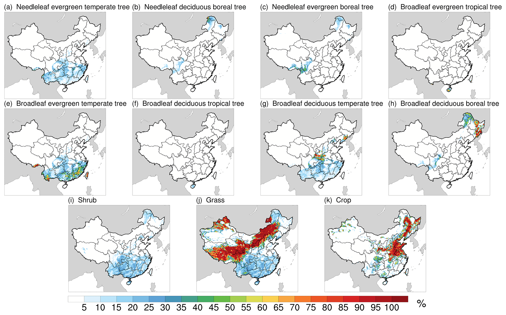
Figure 1The cover fractions of different PFTs for the year 2016.
2.3 Meteorological datasets
The hourly meteorological fields including temperature, downward shortwave radiation (DSW), wind speed, surface pressure, precipitation and water vapor mixing ratio were provided by the Weather Research and Forecast (WRF) model V3.9 (Skamarock et al., 2008) simulations. The model was driven by ERA-Interim reanalysis data (Berrisford et al., 2011) with 27 km horizontal spatial resolution and 39 vertical layers. The physical schemes are presented in Supplement Table S4.
Since light and temperature conditions are the main environmental drivers of BVOC emission (Guenther et al., 1993; Sakulyanontvittaya et al., 2008), we assessed the reliability of the WRF-simulated DSW and 2 m temperature (T2) using in situ observations from 98 radiation observation sites and 697 meteorology observation sites in China. The in situ observations are from the National Meteorological Information Center (http://data.cma.cn/, last access: 25 March 2021). We converted the hourly model outputs and daily observations to monthly averaged values from 2001 to 2016 for comparison. For DSW, the average mean bias (MB), mean error (ME) and root-mean-square error (RMSE) are 40.37 (±20.81), 43.55 (±17.52) and 49.79 (±17.70) W m−2 for 98 studied sites. The overestimation of DSW simulation is a common issue in multiple simulation studies and may be induced by the lack of physical processes for aerosol radiation effect (Wang et al., 2011; Situ et al., 2013; Wang et al., 2018) and misrepresentation of the radiative effect of the sub-grid-scale cumulus cloud (Ruiz-Arias et al., 2016). For T2, the average MB, ME and RMSE are −1.19 (±2.87), 2.40 (±2.14) and 2.65 (±2.11) ∘C among 697 sites over China. The regional-scale validation was also conducted in five main regions (Fig. S1) by comparing the averaged values of the observation and the simulation among the sites in the regions we defined, and the results (Figs. S2 and S3) and statistical parameters (Tables S5 and S6) can be found in the Supplement.
We also compared the monthly anomalies of DSW and T2 from the model simulation and observation to validate the interannual variability of meteorological fields simulated by WRF. As shown in Fig. 2, the results indicate that the model accurately reproduced the interannual variability of DSW and T2, and the correlation coefficients of DSW and T2 anomaly between the simulation and observation reached 0.77 and 0.88, respectively. The trends in growing-season-averaged T2 and DSW from model results as well as in situ measurements are presented in Fig. 3. The model and the in situ measurements show similar patterns of T2. For instance, the model and observations both show an increasing trend in regions like the Tibetan Plateau and southern China as well as a decreasing trend in eastern and northeastern China. For DSW, the model presented a dimming trend in northeastern and eastern China and a brightening trend in southeastern and central China, and the limited number of radiation observation sites show a similar pattern of trend as model results. In general, the WRF simulation successfully captured the long-term meteorological variabilities and is reasonable to use for estimating the impact of climatic variability on BVOC emission in China for this study.
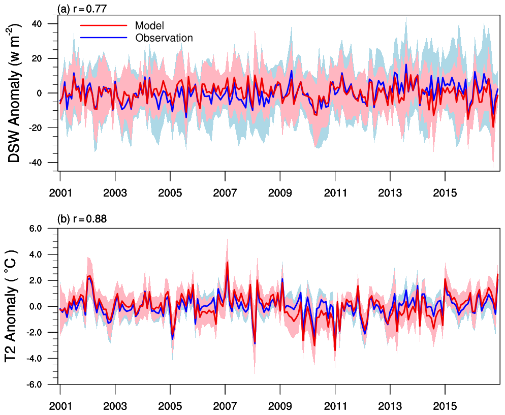
Figure 2The comparison of monthly anomaly of downward shortwave (DSW) radiation (a) and 2 m temperature (T2) (b) for model simulation and in situ observation, and the filled areas present the standard deviations among 98 sites for DSW and 697 sites for T2.
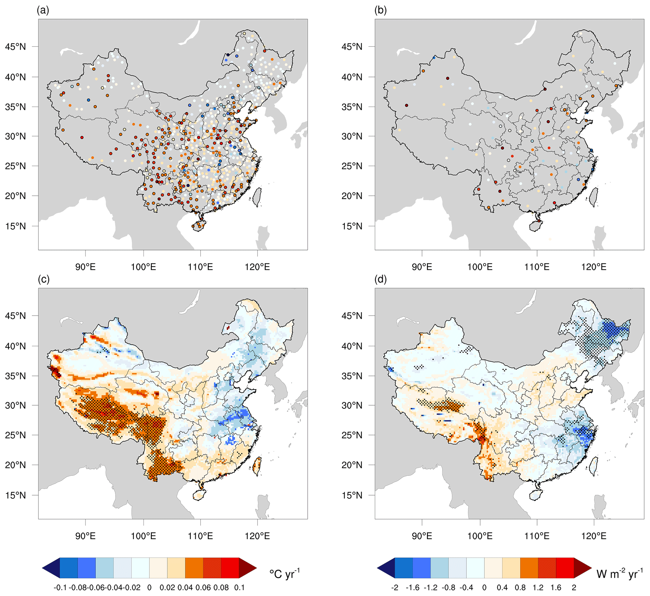
Figure 3The trend of growing-season-averaged 2 m temperature (T2) and downward shortwave radiation (DSW). Panels (a) and (b) are for in situ T2 and DSW, respectively, and the sites with a statistically significant trend are marked by black circles. Panels (c) and (d) are for the WRF-simulated T2 and DSW, respectively, and the regions with statistically significant trends are illustrated by shadow.
2.4 Satellite formaldehyde (HCHO) observations
The satellite HCHO VC used in this study is from the Belgian Institute for Space Aeronomy (BIRA-IASB) and was retrieved using the differential optical absorption spectroscopy (DOAS) algorithm (De Smedt et al., 2012, 2015). We used the monthly Level-3 HCHO VC product with 0.25∘ × 0.25∘ spatial resolution, and the rows affected by the row anomaly since June 2007 have been filtered in this product (De Smedt et al., 2015; Jin and Holloway, 2015). Since the OMI instrument is temporally stable (Dobber et al., 2008; De Smedt et al., 2015), the OMI HCHO VC product is suitable for long-term analysis (Jin and Holloway, 2015) and was used to primarily validate our estimation of isoprene emission variability. The major sources of tropospheric HCHO are biogenic VOCs, anthropogenic VOCs and open fires (Zhu et al., 2017a). Since biogenic isoprene is the dominant source of HCHO over forests in summertime (Palmer et al., 2003), we used HCHO as the proxy of isoprene to validate the interannual variability of isoprene estimates.
2.5 Scenarios and analysis method
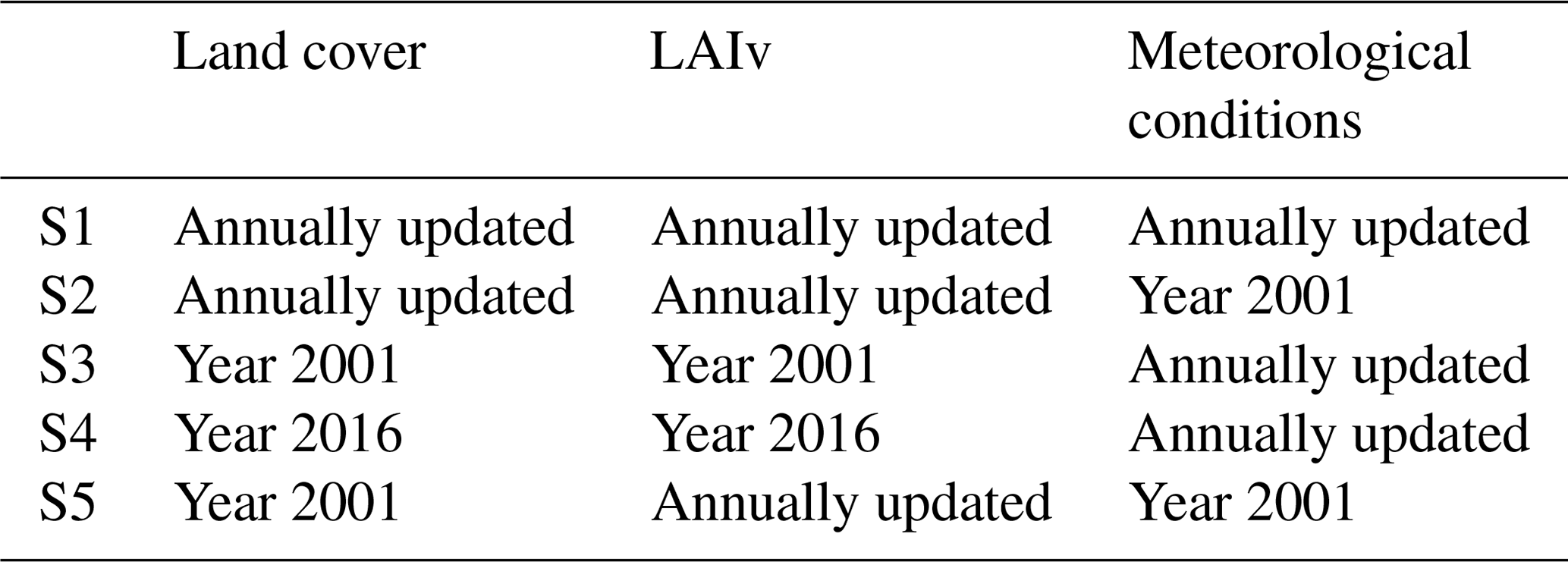
We designed five scenarios (S1–S5) to investigate the impact of land cover change and climatic conditions on BVOC emission. The configurations of the five scenarios are shown in Table 1.
-
S1 was considered as the standard or full scenario.
-
S2 was used to investigate the impact of the ecosystem and land cover variability on BVOC emission.
-
S3 and S4 characterize the effect of climate variability and compare the difference of BVOC emission induced by vegetation change between 2001 and 2016.
-
S5 investigates the contribution of solely the LAI trend to the BVOC emission trend.
The climatic variability can affect the growth of vegetation and then affect LAI values (Piao et al., 2015). In this study, the interaction between climate and ecosystem is not considered in offline MEGAN, which means that the meteorological conditions, e.g., precipitation, will not affect the LAI values or phenology of vegetation.
Table 1Description of different scenarios used to estimate the BVOC emission.
The chemical species emissions estimated by MEGAN were grouped into four major categories including isoprene, monoterpene, sesquiterpene and other VOCs since the terpenoids account for the majority of total BVOC emission and have known impacts on atmospheric oxidants and SOA (Wang et al., 2011). The trend analysis in this study was done following the Theil–Sen trend estimation method, and the results were tested by the Mann–Kendall non-parametric trend test (MK test) (Gilbert, 1987). The trend analysis and the MK tests in this study were implemented using the trend_manken (https://www.ncl.ucar.edu/Document/Functions/Built-in/trend_manken.shtml, last access: 25 March 2021) function of the NCAR Command Language (NCL, https://www.ncl.ucar.edu/, last access: 25 March 2021).
3.1 The variability of BVOC emission in China from 2001–2016
As shown in Table 2, the average annual emissions from 2001–2016 of isoprene, monoterpene, sesquiterpene and other VOCs estimated from S1 are 15.94 (±1.12), 3.99 (±0.17), 0.50 (±0.03) and 13.84 (±0.78) Tg, respectively. Isoprene is the dominant species and accounts for about half of the total BVOC emission in China. As shown in Fig. 4, the estimated BVOC emission in S2 has a statistically significant increasing trend without considering the annual variability of meteorological conditions. The increasing rates of isoprene, monoterpenes, sesquiterpenes and total BVOC emission in S2 scenarios are 0.64, 0.44, 0.39 and 0.50 % yr−1, respectively. The S1 scenario considers the impact of annual meteorological variability as well as the surface vegetation change, and the BVOC emission in S1 shows an upward trend but did not pass the significance test of p<0.1. There is no significant trend of BVOC emission for S3 or S4, with fixed land cover and annually updated meteorological conditions, which demonstrates that meteorology was not the direct driver of the BVOC emission trend in China during this period. Climatic conditions could affect the BVOC emission indirectly by affecting the growth of vegetation and controlling BVOC emission (Peñuelas et al., 2009), which is not considered in the model used in this study. The estimated total BVOC emission in S5 also has a statistically significant increasing trend of 0.26 % yr−1 (p<0.05) without considering the annual variability of meteorological conditions, which is purely caused by the increase in LAI from 2001–2016. The changing trend of BVOC in the full scenario cannot be treated by the linear summation of trends in other one-factor scenarios. On the one hand, the response of isoprene emission to meteorological conditions is nonlinear (Guenther et al., 1993). On the other hand, the calculation of national-scale total emission amount is affected by the spatial variabilities of vegetation types as well as climatic conditions, and it should not be a linear combination of the two aspects.
Table 2The mean annual emission (Tg) of different species in China from 2001 to 2016. The scenarios S1 to S5 are described in Table 1.
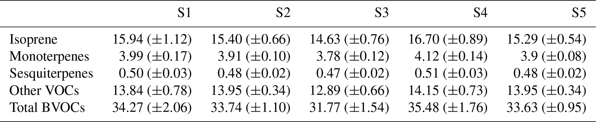

Figure 4Annual BVOC emissions in China from 2001 to 2016 for five scenarios (S1–S5) described in Table 1. The increasing trends and the probabilities (p) using the Mann–Kendall test are shown in the legend.
We also tested the impact of first 2 years on the trend estimation of the national-scale BVOC emission. After removing the first 2 years, the scenarios other than S2 did not show statistically significant trends for most species; however, scenario S2 with the fixed climate inputs of 2001 and the annually updated land cover still showed statistically significant increasing trends for all species (p<0.05), which means the change of land cover is not dominated by the first 2 years.
The surface vegetation change had a significant influence on BVOC emissions in China from 2001–2016 according to our estimation. In S2, the interannual variability of total BVOC emission is primarily determined by the surface vegetation change resulting in a nearly linear increasing trend of BVOC emission. The average annual emission of total BVOC from 2009–2016 is 3.9 % (1.29 Tg) higher than that from 2001–2008 in S2, and the average annual emissions of isoprene, monoterpene and sesquiterpene during the previous 8 years are 5.0 % (0.75 Tg), 3.5 % (0.13 Tg) and 3.1 % (0.02 Tg) higher than those during the next 8 years, respectively. The comparison of S3 and S4 results further demonstrates the importance of vegetation development on BVOC emission considering the interannual variability of meteorological conditions. S3 and S4 adopted the same annually updated meteorological field but with the fixed land cover information of the years 2001 and 2016, respectively. The fluctuation of meteorological factors leads to an interannual variability of BVOC emission in S3 and S4, but the increase in vegetation cover rate in 2016 results in BVOC emissions that are much higher than those in 2001. As presented in Table 2, the average total BVOC emissions are 31.77 (±1.54) and 35.48 (±1.76) Tg in S3 and S4, respectively, and the total BVOC emission in S4 is 11.7 % (3.71 Tg) higher than that in S3. The emissions of isoprene, monoterpene and sesquiterpene with the land cover information of the year 2016 are 14.1 % (2.07 Tg), 9.0 % (0.34 Tg) and 8.5 % (0.04 Tg) higher than those estimated based on the land cover information of the year 2001, respectively.
3.2 The regional variability of BVOC emission in China
The hotspots of BVOC emission are mainly located in northeast, central and south China where the forest is widely distributed and the climate is warm and favorable for emitting BVOCs as shown in Fig. 5. The Changbai Mountains, the Qin Mountains, the southeast and southwest China forest regions, southeast Tibet, and Hainan and Taiwan islands are the regions with the highest BVOC emission in 2001. The spatial patterns of statistically significant (p<0.1) changing trends in S1–S5 are also presented for individual categories in Fig. 5. The spatial distributions of trends of different species in S2 all show a significantly increasing trend in the regions including northeast, central and south China since the vegetation development is the main driver of the increasing trend of BVOC emission (c, i, o and u in Fig. 5). In the full scenario of S1, the area with statistically significant trend is less than that in S2 considering the impact of meteorological variability. S5 also shows a nationwide significantly increasing trend of BVOC emission but with smaller rates compared to S2 (f, l, r and x in Fig. 5). A positive increasing trend induced by meteorology is also found in Tibet, western Sichuan and southeastern Yunnan Province in S3 and S4, which is induced by the warming climate and stronger DSW as presented in Fig. 3.

Figure 5The horizontal distributions of isoprene, monoterpenes, sesquiterpenes and total BVOCs emissions of China in 2001 are shown in panels (a), (g), (m) and (s), respectively. The rest of the rows present the changing trend of isoprene (b–f), monoterpenes (h–l), sesquiterpenes (n–r) and total BVOCs (t–x) in S1, S2, S3, S4 and S5, respectively. The Mann–Kendall test was used to mark the grids where p is smaller than 0.1.
The spatial patterns of changing trends of total BVOC emission and land cover parameters are presented in Fig. 6. The cover fraction of broadleaf trees shows a strong increasing trend in the regions including northeastern, central and southern China. Meanwhile, the grass and crop cover fractions show a decreasing trend in these regions. The crop cover rate also shows an increasing trend in northeastern China, Shan Xi, Gansu and Xinjiang provinces by replacing the grass there. Besides the change of PFTs, a nationwide increasing trend of LAIv was also found for most regions in China.

Figure 6Spatial distribution of total BVOC emission in 2001 (a) and the changing trends of annual emission flux (S1, S2 and S5) and cover fractions of the main PFTs and LAIv. The Mann–Kendall test was used to filter the grids where p is greater than 0.1.
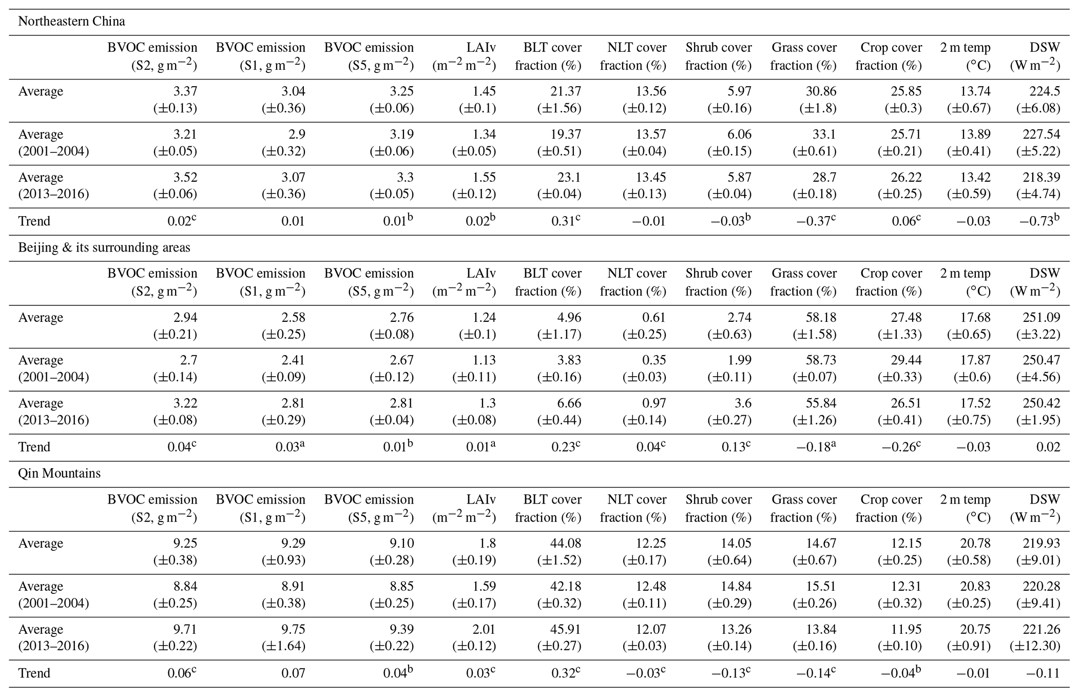
In order to understand the regional discrepancies of the changing trend of BVOC emission and its drivers, we chose six regions of interest to further analyze. Our selection is based on the changing trends we found from Figs. 5 and 6. We did not use the geographical boundaries as the criteria to select the regions of interest, and we chose the hotspots with positive trends and investigated the drivers of trends in these regions. As shown in (a) of Fig. 6, the six regions include (1) northeastern China (orange frame in Fig. 6a, 45.5–54∘ N, 118–130∘ E), (2) Beijing and its surrounding areas (black frame in Fig. 6a, 39–42.5∘ N, 114–120∘ E), (3) Qin Mountains (red frame in Fig. 6a, 30–34∘ N, 105.5–112∘ E), (4) Yunnan Province (blue frame in Fig. 6a, 21–27∘ N, 97.5–106∘ E), (5) Guangxi–Guangdong provinces (purple frame in Fig. 6a, 21–25∘ N, 106–117∘ E), and (6) Hainan island (green frame in Fig. 6a, 17.5–20.5∘ N, 108–112∘ E). The annual changes of vegetation conditions (PFTs and LAIv), annual emission flux, growing-season-averaged temperature and DSW are presented in Figs. 7 and 8, and the averaged values and trends of the above variables are listed in Tables 3 and 4. In general, six regions all show that woody vegetation replaced herbaceous vegetation with a significantly increasing trend of annual LAIv. Since the broadleaf trees tend to have a higher emission potential than grass or crop (Guenther et al., 2012), the transformation of land cover from grass or crop to broadleaf tree is expected to enhance the emission of BVOC by increasing the landscape average emission factor. As shown in Tables 3 and 4, the broadleaf tree cover fraction increased at a rate of 0.15 % yr−1–0.32 % yr−1, and the grass cover fraction decreased at a rate of 0.11 % yr−1–0.37 % yr−1 among the six regions from 2001–2016. Except for the region of northeastern China that we defined, the other five regions all show a decreasing trend of 0.04 % yr−1–0.26 % yr−1 for the crop cover fraction. As a result, the total tree cover fraction during the last 4 years (2013–2016) is 11.0 %, 82.5 %, 6.1 %, 5.7 %, 5.9 % and 8.0 % higher than that during the first 4 years (2001–2004) for northeastern China, Beijing and its surroundings, Qin Mountains, Yunnan Province, Guangxi–Guangdong provinces, and Hainan Island, respectively, and the LAIv for these regions also increased by 14.8 %–26.4 %. Correspondingly, the annual BVOC emission flux in all six regions shows a significantly increasing trend without considering the variability of meteorology in S2. The mean annual BVOC emission flux for the last 4 years (2013–2016) is 8.6 %–9.8 % higher than that for the first 4 years (2001–2004) in the regions defined above except for Beijing and its surrounding areas, where the change of the annual BVOC emission flux reached 19.3 %, with the tree cover fraction increasing by 82.5 %. If we only consider the contribution of LAI change, as described in scenario S5, the above subregions except for Guangxi–Guangdong provinces still show a statistically significant increasing trend of BVOC emission without considering the variability of meteorology, and the increasing trend of contributions of the LAIv change to BVOC emission is about 25 %–66 % in these regions.
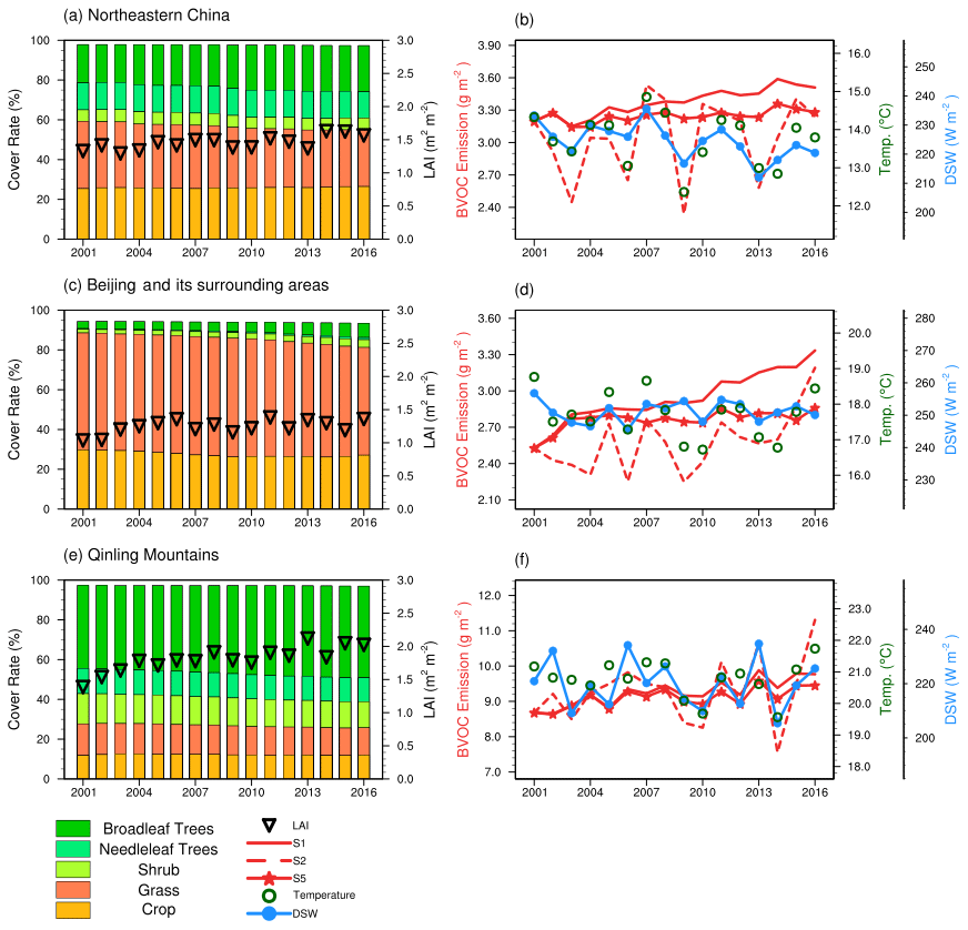
Figure 7The annual changes of PFTs and the annual emission amount of BVOC and LAI in (a) northeastern China, (b) Beijing and its surroundings, and the (c) Qin Mountains. The solid, dashed and marked lines represent the mean emission flux rate of total BVOC in S1, S2 and S5, respectively.
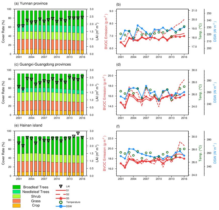
Figure 8The annual changes of PFTs and the annual emission amount of BVOC and LAI in (a) southwestern China, (b) southern China and (c) Hainan island. The solid, dashed and marked lines represent the mean emission flux rate of total BVOC in S1, S2 and S5, respectively.
Table 3The change and trend of annual emission flux (S1, S2 and S5), cover fractions of the main PFTs, LAIv, growing season temperature and DSW in northeastern China, Beijing and its surrounding areas, and the Qin Mountains.
a p<0.1. b p<0.05. c p<0.01.
Table 4The change and trend of annual emission flux (S1, S2 and S5), cover fractions of the main PFTs, LAIv, growing season temperature and DSW in Yunnan Province, Guangxi–Guangdong provinces and Hainan island.
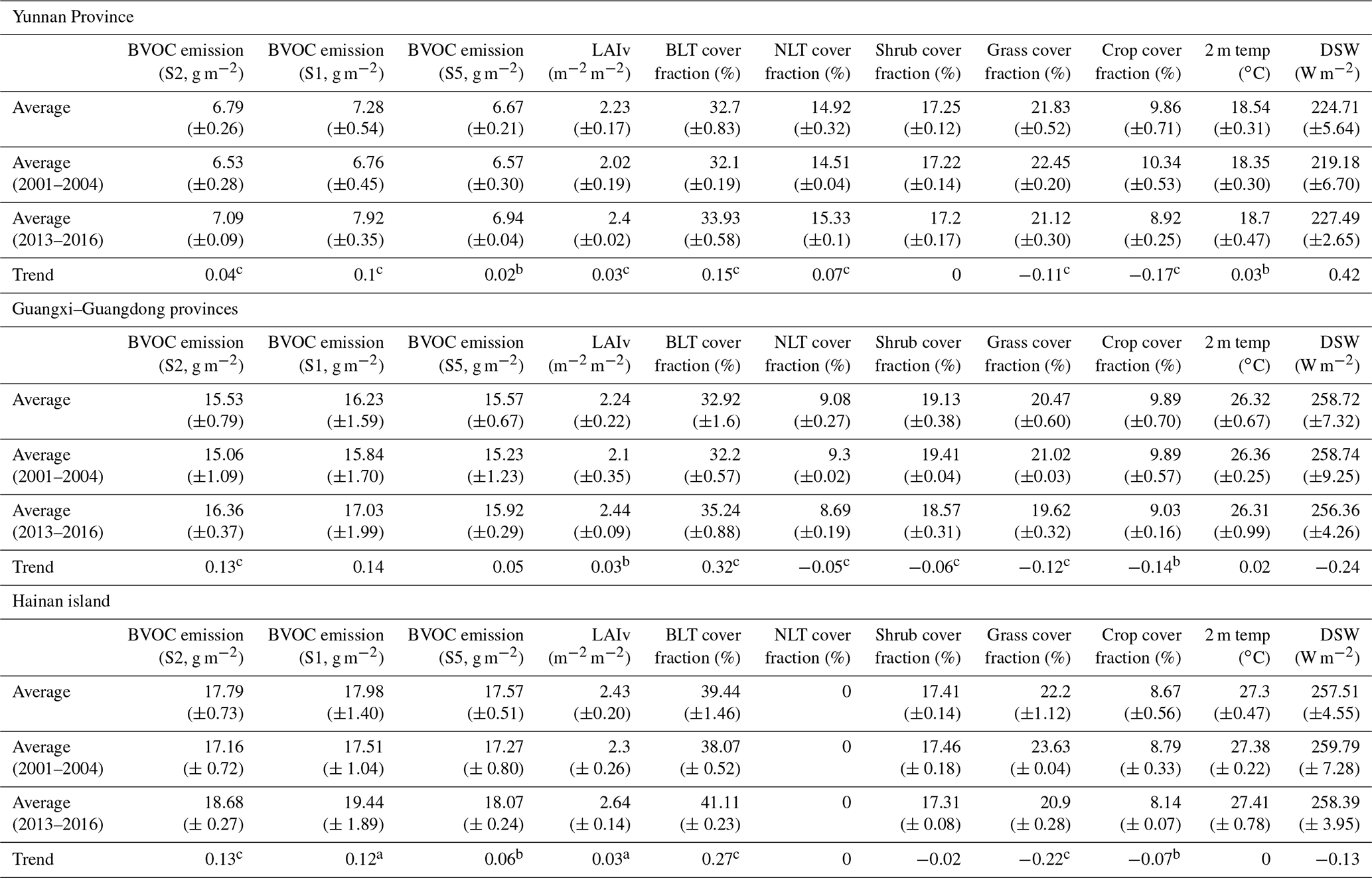
a p<0.1. b p<0.05. c p<0.01.
The changing trend of the annual BVOC emission flux is different in S1 when the impact of meteorological variability is taken into account. The simulated T2 and DSW during the growing season do not show a significant trend in most regions we chose. As shown in Figs. 7 and 8, the variabilities of the temperature and DSW during the growing season controlled the variability of BVOC flux in S1. When the meteorological variability is considered, there are still three regions we defined above that show a significantly increasing trend of BVOC emission: (1) Beijing and its surrounding areas, (2) Guangxi–Guangdong provinces, and (3) Hainan island. In Beijing and its soundings, the changing trend of the annual BVOC emission flux is 0.03 g m−1 yr−1 in S1, and the mean annual BVOC emission flux in the last 4 years still shows a large increase of 16.6 % compared to that in the first 4 years in this region. A significantly increasing trend of temperature of 0.03 ∘C yr−1 was found in southwestern China; therefore, the increasing trend of the annual BVOC emission flux is 0.1 g m−1 yr−1 in S1, which is higher than that in S2 of 0.04 g m−1 yr−1. The BVOC flux in the last 4 years is about 17.2 % higher than that in the first 4 years in southwestern China. In Hainan island, the changing trend of the annual BVOC emission flux is 0.12 g m−1 yr−1 in S1, and the annual BVOC emission flux in the last 4 years is 11.0 % higher than that in the first 4 years.
The estimated increase in BVOC in regions like the Qin Mountains and southern China is expected to affect regional air quality. For the Qin Mountains and surrounding areas, as estimated by Li et al. (2018) using the WRF-Chem model, the average contribution of BVOC to O3 could reach 16.8 ppb for the daily peak concentration and 8.2 ppb for the 24 h concentration in the urban region of Xi'an, one of the biggest cities near the Qin Mountains suffering from poor air quality in recent years (Yang et al., 2019). For Guangxi–Guangdong provinces, Situ et al. (2013) reported that BVOC emission could contribute an average 7.9 ppb surface peak O3 concentration for the urban area in the Pearl River Delta region, and the contribution from BVOC even reached 24.8 ppb over the Pearl River Delta (PRD) in November. Since BVOC plays an important role in local air quality, the change of BVOC emission may have an even greater effect on the local ozone pollution. For instance, the simulation study by Li et al. (2018) also found that the urban region of Xi'an is VOC-limited because of the abundant NOx emissions there. Therefore, the increase in BVOC emission in the Qin Mountains would further favor the formation of O3 in the urban region of Xi'an.
3.3 Comparison of estimates of isoprene emission and satellite-derived formaldehyde column concentration
The OMI HCHO VC product from 2005–2016 developed by BIRA-IASB (De Smedt et al., 2015) was used in this study. The interannual variability of isoprene emission estimated in this study was evaluated by comparing the summer-averaged (June–August) isoprene emission with the summer-averaged HCHO VC.
The annually averaged LAI from 2005–2016 presented in Fig. 9 indicates the spatial distribution of vegetation in China. However, the spatial pattern of estimated isoprene emission (Fig. 9b) differs from the spatial distribution of vegetation because of the variability of emission potentials among different PFTs in MEGAN as well as the climatic conditions. The spatial pattern of average summertime HCHO VC observed by the OMI sensor from 2005–2016 is also presented in Fig. 9c. The highest summer HCHO concentrations in the US are mainly distributed in rural forest regions dominated by biogenic emission (Palmer et al., 2003), while the highest summer HCHO concentrations in China are mainly distributed in developed regions like the North China Plain where HCHO concentration is dominated by anthropogenic sources (Smedt et al., 2010). There is a moderate HCHO VC of about 6–10 × 1015 molec. cm−2 in the vegetation-dominated regions of China.
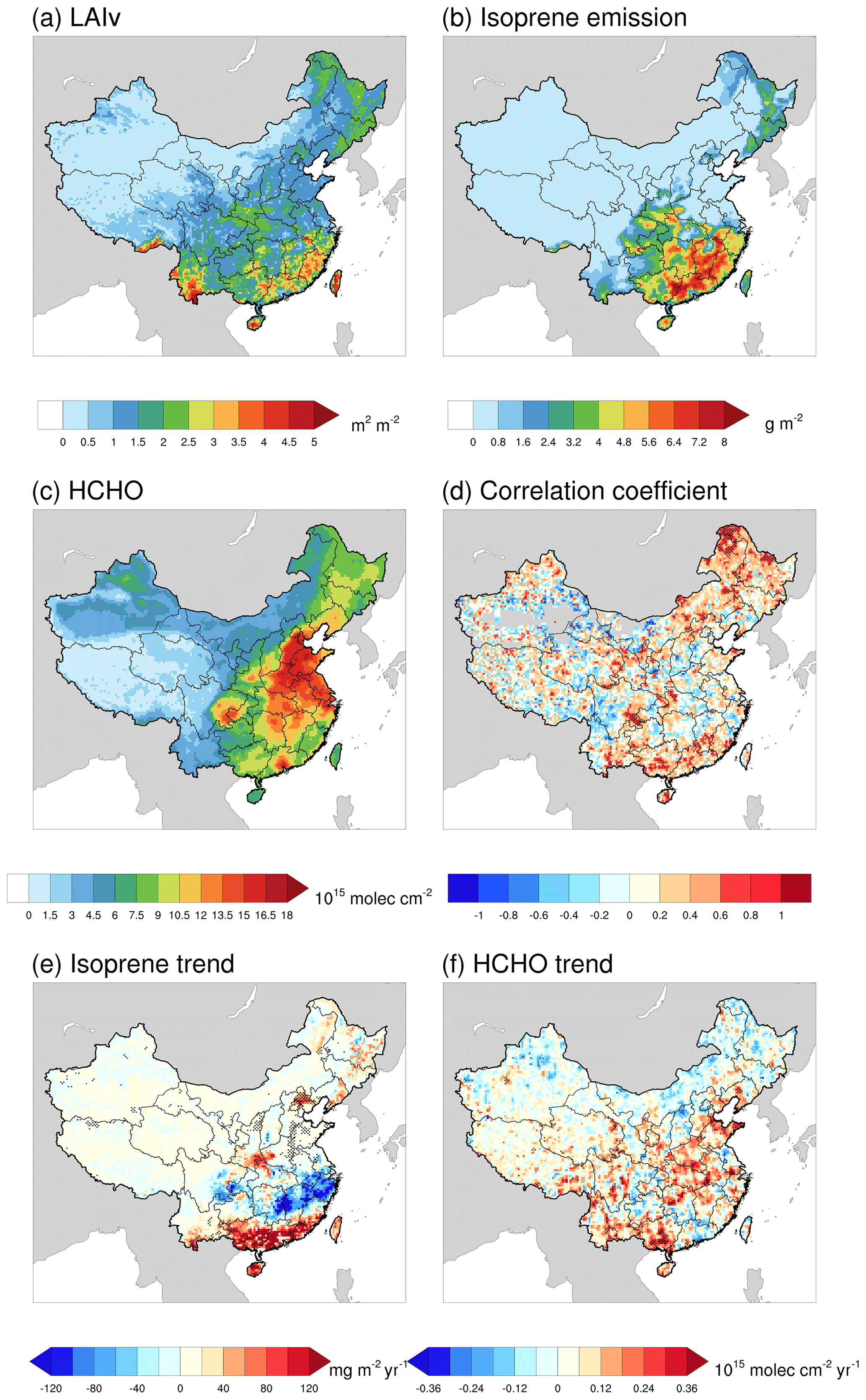
Figure 9Comparison of estimated isoprene annual emission with the satellite-derived tropospheric HCHO vertical column concentration by OMI from 2005–2016. Panels (a), (b) and (c) illustrate the spatial patterns of annual mean LAIv, isoprene emission and HCHO vertical columns (VC) by OMI, respectively. Panel (d) presents the spatial distribution of the correlation coefficient between summertime isoprene emission and HCHO VC. Panels (e) and (f) show the increasing trend of isoprene and HCHO VC from 2005–2016.
The grid level correlation coefficients between the average summer HCHO VC and isoprene emission estimated in our study are shown in Fig. 9d, and the grids with statistically significant correlations (p<0.1, N=12) are marked with black dots. A correlation is found in northeast, central and south China where there are relatively high vegetation cover rates and low anthropogenic influence. In contrast, there is almost no statistically significant correlation in the high-HCHO-VC regions like the North China Plain, which is dominated by anthropogenic emissions. However, the distribution of statistically significant positive correlated points is not completely consistent with the vegetation distribution indicated by LAI due to the absence of consideration of physical and chemical processes, including transportation, diffusion and chemical reactions. The grids with significant correlation are mostly distrusted in or near rural regions with high vegetation biomass, indicating that our estimations can represent the annual variation in isoprene emission.
The increasing trends of isoprene and HCHO VC from 2005–2016 are presented in e and f of Fig. 9, and the statistically significant (p<0.1) grids are marked with black dots. The increasing trend pattern of isoprene emission from 2005–2016 is basically consistent with that from 2001–2016, which has been described in Sect. 3.2, and it is clear that southern China is the region with the strongest positive trend. For HCHO, developed regions such as the North China Plain have an increasing trend because of the increase in human activities (Smedt et al., 2010), there is also an obvious increasing trend of HCHO VC at Yunnan and Guangxi provinces in the south of China. Moreover, these regions, especially Guangxi Province, also show a statistically significant positive correlation between isoprene emission and HCHO VC as presented in Fig. 9d. This implies that biogenic emissions might be the main driver of the increased HCHO in Guangxi Province; however, the absence of physical and chemical processes like transport led to a large uncertainty to this conclusion. Here we conducted a primary comparison between HCHO VC and isoprene emission, and a more thorough study by using a chemical transport model may help to further explain the relationship between the variability of HCHO VC and isoprene emission in the future.
3.4 Comparison with other studies and discussion of uncertainties
The comparison of isoprene and monoterpene emission estimations between our study and previous studies is presented in Table 5. The estimations of isoprene emission range from 4.65 to 33.21 Tg, and the estimations of monoterpene emission range from 3.16 to 5.6 Tg in China. Multiple factors including emission factor, meteorology and land cover inputs can lead to the discrepancy of these estimations. We listed the inputs of these estimations in Table 6 to fully understand the discrepancies between our results and other estimations.
Table 5Comparison of isoprene and monoterpene emissions (Tg) in China with previous studies.
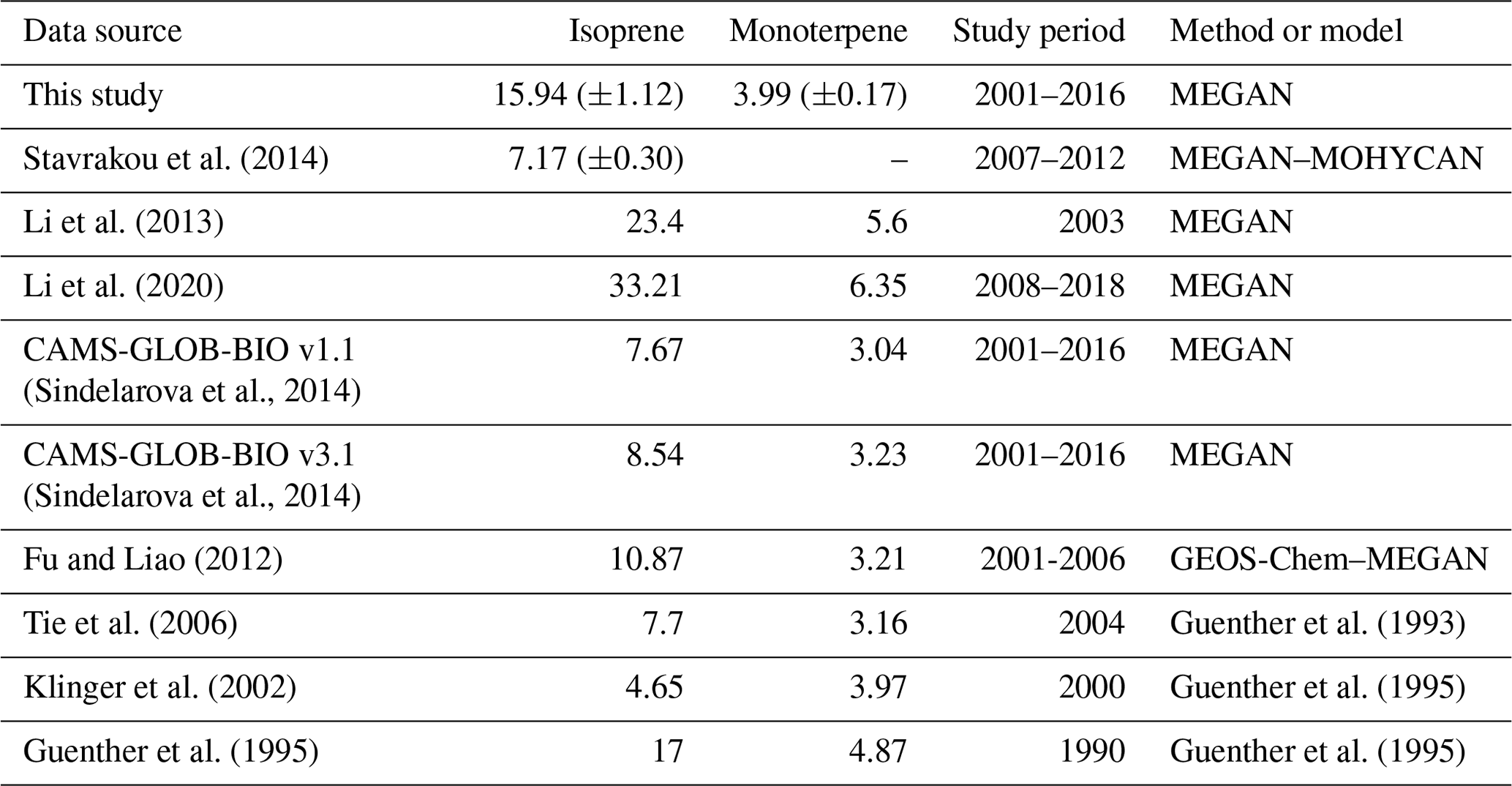
Table 6Comparison of inputs for BVOC estimation with previous studies.

The setting of inputs in this study is relatively close to the study by Stavrakou et al. (2014) and CAMS-GLOB-BIO biogenic emission inventories (https://eccad3.sedoo.fr/#CAMS-GLOB-BIO, last access: 25 March 2021) that adopted the method described by Sindelarova et al. (2014). However, the estimation of isoprene emission in this study is about 86.6 %–122.3 % higher than their estimations, and the estimation of monoterpene emission is about 23.5 % and 31.3 % higher than that from CAMS-GLOB-BIO v3.1 and v1.1, respectively. We further compared our results with two versions of CAMS-GLOB-BIO inventories. Figures 10 and 11 present the trends of isoprene emission and monoterpene emission, respectively, from S1 and S3 in this study and the CAMS-GLOB-BIO inventory v1.1 and v3.1 from 2001–2016. As shown in Figs. 10 and 11, S3 shows similar spatial patterns and magnitude of the changing trend of isoprene and monoterpene emissions as CAMS-GLOB-BIO v1.1 and CAMS-GLOB-BIO v3.1, e.g., three datasets all showed a strong increasing trend in Yunnan Province, and S1 shows much stronger changing trends comparing with the other three datasets with annually updated LAI and PFT datasets. The meteorological inputs for CAMS-GLOB-BIO v1.1 and v3.1 are ERA-Interim and ERA-5 reanalysis data, respectively, and the WRF model used in this study was also driven by ERA-Interim reanalysis data. Therefore, the four datasets have the same source of meteorological inputs. In addition, these estimations all adopted the same PFT-level emission factors from Guenther et al. (2012). Therefore, the potential reason for the differences of isoprene and monoterpene emission among the datasets in Figs. 10 and 11 is the discrepancies of PFT and LAI inputs. CAMS-GLOB-BIO also adopted the annually updated LAI inputs developed by Yuan et al. (2011) based on the MODIS MOD15A v5 LAI product, but the two versions of the CAMS-GLOB-BIO inventory did not show the same level of strong increasing trend as S1. The increasing trend of LAI in China is confirmed by multiple LAI products but with different rates (Piao et al., 2015; Chen et al., 2020). In this study, we adopted the latest MODIS LAI product of version 6, and a strong increasing trend of LAI in China has been found by using this product (Chen et al., 2019). Therefore, an increasing trend of BVOC emission induced by LAI should be seen in the estimation with annually updated LAI inputs, but the magnitude of this trend is also affected by the magnitude of changing trend of LAI products. The PFT map used in this study is coming from the MODIS land cover product, which is a mesoscale satellite product with the highest resolution of 500 m. Besides the quality of the product, the method for converting the original land cover classification system to a PFT classification system is also important. Hartley et al. (2017) illustrated that the cross-walking table for converting land cover class maps to PFT fractional maps can lead to 20 %–90 % uncertainties for gross primary production estimation in land surface models by using different vegetation fractions for mixed pixels, and the BVOC emission estimation has the same issue. In this study, we assumed that the pixels that were assigned as vegetation are 100 % covered by that kind of vegetation (Table S1 in the Supplement). Therefore, this will lead to an overestimation of vegetation cover rate for mixed pixels, which can lead to higher BVOC emission.
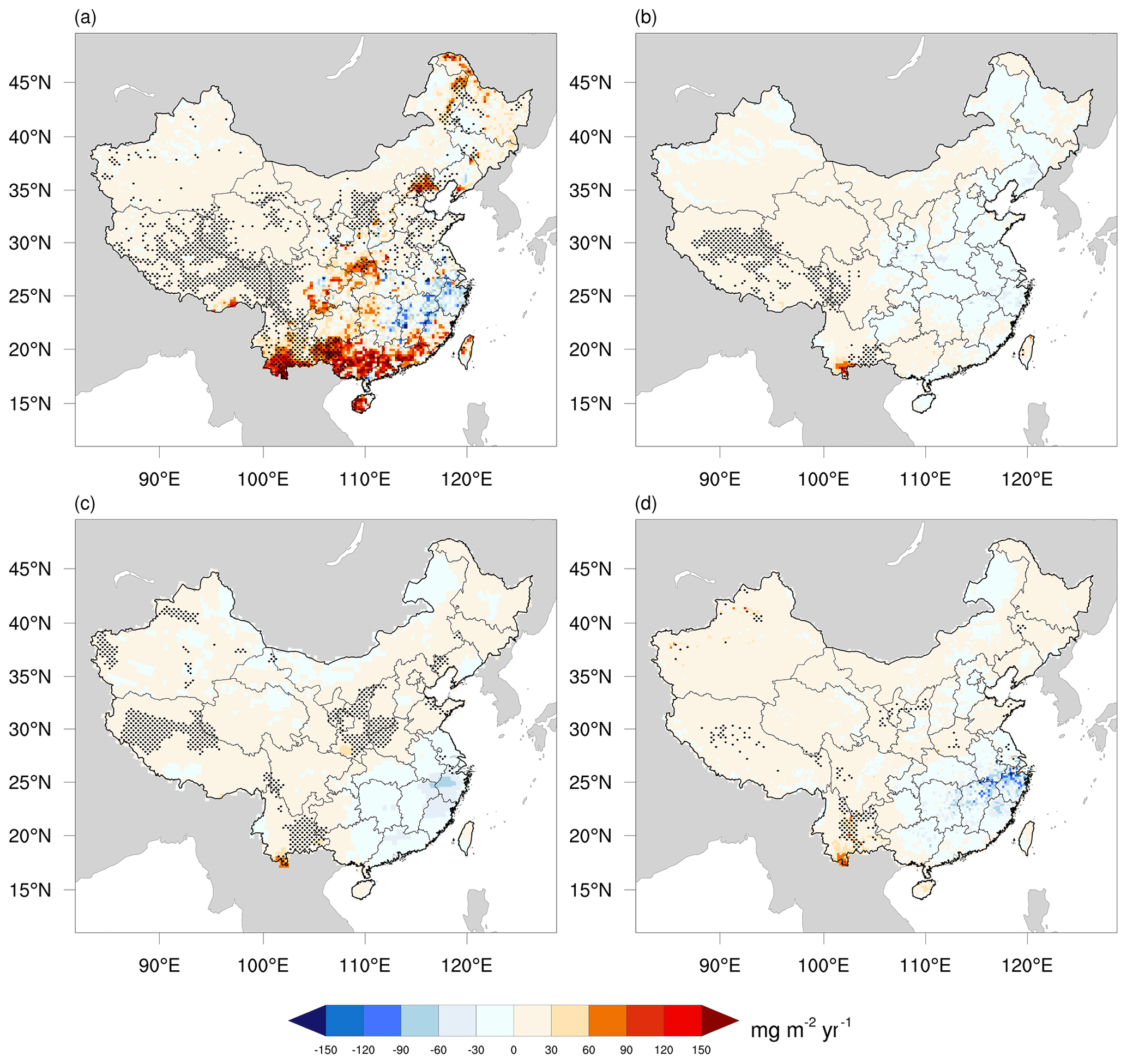
Figure 10Comparison of the trend of isoprene emission between this study (S1) and other estimations from 2001–2016. Panels (a) and (b) are for S1 and S3, respectively, in this study, and (c) and (d) are for CAMS-GLOB-BIO v1.1 and CAM-GLOB-BIO v3.1, respectively. The Mann–Kendall test was used to mark the grids where p is smaller than 0.1.
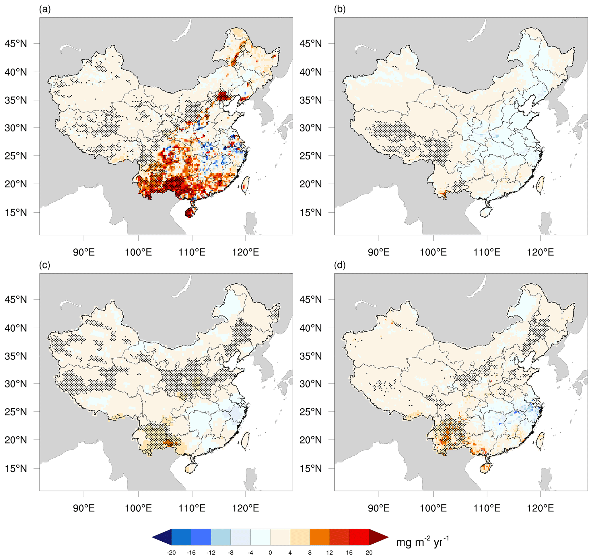
Figure 11Comparison of the trend of monoterpene emission between this study (S1) and other estimations from 2001–2016. Panels (a) and (b) are for S1 and S3, respectively, in this study, and (c) and (d) are for CAMS-GLOB-BIO v1.1 and CAM-GLOB-BIO v3.1, respectively. The Mann–Kendall test was used to mark the grids where p is smaller than 0.1.
The emission factor is also an important source of uncertainties, and it decided the spatial patterns of emission rates together with the PFT distribution. In order to understand the role of the emission factor, the flux measurements of isoprene and monoterpenes from the campaigns conducted from 2010 to 2016 in China (Bai et al., 2015, 2016, 2017) were collected and compared with model results in this study. The details of these campaigns are provided in Table 7, and the emission factors that were retrieved from the observations are also listed for these sites. Most samples were collected during the daytime every 3 h according to the descriptions of the measurements (Bai et al., 2015, 2016, 2017); therefore, we averaged the model results from 08:00 to 20:00 in local time with a 3 h interval for comparison. As shown in (a) and (b) of Fig. 12, the modeled fluxes of isoprene and monoterpenes with the default emission factors in this study did not capture the variability of the observations. The ME, MB and RMSE are 1.60, 1.59 and 2.31 mg m−2 h−1 for isoprene and 0.21, −0.003 and 0.32 mg m−2 h−1 for monoterpenes. When we adopted the emission factors retrieved from observations (Bai et al., 2015, 2016, 2017), the simulated isoprene and monoterpene fluxes showed relatively good consistence with the observations by using the same activity factor from the model (γ in Eq. 1) as shown in (c) and (b) of Fig. 12. The ME, MB and RMSE are 0.44, 0.41 and 0.57 mg m−2 h−1 for isoprene and 0.32, 0.14 and 0.49 mg m−2 h−1 for monoterpenes after adopting the observation-based emission factors, and the statistic parameters for isoprene simulation are largely improved. Although the MB and ME of monoterpene simulation increased, the simulated monoterpene flux shows better agreement with observations (Fig. 12). Therefore, it is clear that our calculation of activity factors is in a reasonable range, but the emission factor is the main source of uncertainties. The PFT-level emission factors used in this study from Guenther et al. (2012) represent the globally averaged emission factor for PFTs, and it is relatively easy to use them with the satellite PFT products. Therefore, most studies listed in Table 6 adopted the PFT or land use emission factors. Our validation showed that an accurate emission factor based on observations could largely improve the performance of MEGAN, but it also requires abundant efforts to conduct measurements. However, the measurements listed in Table 7 are still very limited for describing the spatial discrepancies of ecosystems in China, so we still used the default emission factors in MEGAN for our national-scale estimation. The estimations by Li et al. (2013, 2020) used the species-level emission factors and vegetation atlas of China for 2007 to describe the spatial distribution of BVOC emission potentials, and they concluded the reason why their estimations were far higher than other studies is the high emission factors they adopted. Therefore, the same validations by using canopy-scale BVOC flux measurements are also needed for these studies to validate and constrain the emission factors they used.
Table 7Detailed descriptions of the flux measurements used in this study and corresponding campaigns.

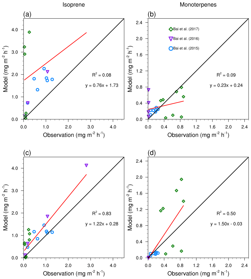
Figure 12Validation of the model with flux measurements in China. Panels (a) and (b) show the performance of MEGAN with the default emission factors (N=19). Panels (c) and (d) show the performance of MEGAN with the emission factors derived from observations (N=19).
Meteorological input is also a source of uncertainties for BVOC emission estimation. As shown in Fig. 12, the modeled isoprene and monoterpene fluxes are still generally higher than observations when observation-based emission factors were used. One potential reason for this phenomenon is the overestimation of temperature and radiation as described in Sect. 2.3. The sensitivity tests by Wang et al. (2011) showed that the 1.89 ∘C discrepancy of temperature can result in −19.2 % to 23.2 % change of isoprene emission and −16.2 % to 18.5 % change of monoterpene emission for the Pearl River Delta region in July, which is also a hotspot for BVOC emission in this study. They also found that 115.8 W m−2 discrepancy of DSW can result in −31.4 % to 36.2 % change of isoprene emission and −14.3 % to 16.8 % change of monoterpene emission for the same region. The BVOC emission in this study might be overestimated because of the overestimated temperature and DSW in meteorological inputs. However, inaccurate emission factors could lead to over 100 % uncertainties, which is more significant than the uncertainties induced by meteorological inputs.
Satellite observations have shown that China has led the global greening trend in recent decades (Chen et al., 2019). In this study, we investigated the impact of this greening trend on BVOC emission in China from 2001 to 2016. We used long-term satellite vegetation products as inputs in MEGAN. According to the estimation of the model, we found the greening trend of China is leading a national-scale increase in BVOC emission. The BVOC emission level in 2016 could be 11.7 % higher than that in 2001 because of higher tree cover fraction and biomass. The comparison among different scenarios showed that vegetation changes resulting from land cover management are the main driver of BVOC emission change in China. Climate variability contributed significantly to interannual variations but not much to the long-term trend during the study period.
On regional scales, there are strong increasing trends in (1) northeastern China, (2) Beijing and its surrounding areas, (3) the Qin Mountains, (4) Yunnan Province, (5) Guangdong–Guangxi provinces, and (6) Hainan island. A strong increasing trend of broadleaf tree cover fractions and LAIv was found in these regions. The mean total tree cover fraction during the last 4 years (2013–2016) is 5.7 %–82.5 % higher than that of the first 4 years (2001–2004) for these regions, and the LAIv from 2013–2016 increased by 14.8 %–26.4 % compared to that from 2001–2004 in these regions. Consequently, the average BVOC emission flux for the last 4 years (2013–2016) is 8.6 %–19.3 % higher than that for the first 4 years (2001–2004) in the subregions we defined driven by the same meteorological inputs. In the standard scenario of S1, a statistically significant increasing trend could still be found in the subregions including Beijing and its surroundings, Yunnan Province, and Hainan island when the climate variability was considered.
We used the long-term record of satellite HCHO VC from the OMI sensor to assess our estimation of isoprene emission in China from 2005–2016. The results indicated statistically significant positive correlation coefficients between the isoprene emission estimate and satellite HCHO VC in summer over the regions with a high vegetation cover fraction including northeast, central and southern China. In addition, isoprene emission and HCHO VC both had a statistically significant increasing trend in the south of China, mainly Guangxi Province, where there was a statistically significant positive correlation supporting the estimated variability of BVOC emission in China. However, the absence of the physical and chemical processes, e.g., transport, led to a large uncertainty in this conclusion, and a more thorough study using a chemical transport model may help to further explain the relationship between the variability of HCHO VC and the isoprene emission.
We conclude that uncertainties of this study mainly come from the emission factor, PFT and LAI inputs through comparing our results with other studies and flux measurements from 2010–2016 in China. The validation with flux measurements suggested that using the observation-based emission factor could largely improve the performance of the model, but it also requires much more effort. Our results suggest that the continued increase in BVOC will enhance the importance of considering BVOC when making policies for controlling ozone pollution in China along with ongoing efforts to increase the cover fraction of forest.
The source code of MEGAN v2.1 is available at https://bai.ess.uci.edu/megan/data-and-code/megan21 (last access: 25 March 2021; Guenther et al., 2006, 2012). The MODIS MCD12C1 land cover product Version 6, MODIS MCD15A2 LAI Version 6 and MODIS MOD44B VCF Version 6 datasets are available on the website of the Land Processes Distributed Active Archive Center (LP DAAC) at https://lpdaac.usgs.gov/dataset_discovery/modis/modis_products_table (last access: 25 March 2021). The version 14 Level 3 OMI HCHO VC products were downloaded from the website of the Tropospheric Emission Monitoring Internet Service (TEMIS) at http://h2co.aeronomy.be (last access: 25 March 2021; De Smedt et al., 2012, 2015).
The supplement related to this article is available online at: https://doi.org/10.5194/acp-21-4825-2021-supplement.
QW, LW and HW planned and organized the project. HW, JF and QX prepared the input datasets. HW modeled and analyzed the data. HW and QW wrote the manuscript. HW, ABG and QW revised the manuscript. ABG, XY, LW, TX, JL, JF and HC reviewed and provided key comments on the paper.
The authors declare that they have no conflict of interest.
The National Key R&D Program of China (2017YFC0209805 and 2016YFB0200800), the National Natural Science Foundation of China (41305121), the Fundamental Research Funds for the Central Universities and Beijing Advanced Innovation Program for Land Surface funded this work. The research is support by the High Performance Scientific Computing Center(HSCC) of Beijing Normal University. The authors thank the topical editor and the anonymous referees for their valuable comments.
This research has been supported by the National Key R&D Program of China (grant nos. 2017YFC0209805 and 2016YFB0200800), the National Natural Science Foundation of China (grant no. 41305121), the Fundamental Research Funds for the Central Universities and Beijing Advanced Innovation Program for Land Surface.
This paper was edited by Eleanor Browne and reviewed by two anonymous referees.
Arneth, A., Niinemets, Ü., Pressley, S., Bäck, J., Hari, P., Karl, T., Noe, S., Prentice, I. C., Serça, D., Hickler, T., Wolf, A., and Smith, B.: Process-based estimates of terrestrial ecosystem isoprene emissions: incorporating the effects of a direct CO2-isoprene interaction, Atmos. Chem. Phys., 7, 31–53, https://doi.org/10.5194/acp-7-31-2007, 2007.
Bai, J., Guenther, A., Turnipseed, A., and Duhl, T.: Seasonal and interannual variations in whole-ecosystem isoprene and monoterpene emissions from a temperate mixed forest in Northern China, Atmos. Pollut. Res., 6, 696–707, https://doi.org/10.5094/APR.2015.078, 2015.
Bai, J., Guenther, A., Turnipseed, A., Duhl, T., Yu, S., and Wang, B.: Seasonal variations in whole-ecosystem BVOC emissions from a subtropical bamboo plantation in China, Atmos. Environ., 124, 12–21, https://doi.org/10.1016/j.atmosenv.2015.11.008, 2016.
Bai, J., Guenther, A., Turnipseed, A., Duhl, T., and Greenberg, J.: Seasonal and interannual variations in whole-ecosystem BVOC emissions from a subtropical plantation in China, Atmos. Environ., 161, 176–190, 10.1016/j.atmosenv.2017.05.002, 2017.
Bauwens, M., Stavrakou, T., Müller, J.-F., Van Schaeybroeck, B., De Cruz, L., De Troch, R., Giot, O., Hamdi, R., Termonia, P., Laffineur, Q., Amelynck, C., Schoon, N., Heinesch, B., Holst, T., Arneth, A., Ceulemans, R., Sanchez-Lorenzo, A., and Guenther, A.: Recent past (1979–2014) and future (2070–2099) isoprene fluxes over Europe simulated with the MEGAN–MOHYCAN model, Biogeosciences, 15, 3673–3690, https://doi.org/10.5194/bg-15-3673-2018, 2018.
Berrisford, P., Dee, D. P., Poli, P., Brugge, R., Mark, F., Manuel, F., Kållberg, P. W., Kobayashi, S., Uppala, S., and Adrian, S.: The ERA-Interim archive Version 2.0, ECMWF, Shinfield Park, Reading, 2011.
Bonan, G. B., Levis, S., Kergoat, L., and Oleson Keith, W.: Landscapes as patches of plant functional types: An integrating concept for climate and ecosystem models, Global Biogeochem. Cy., 16, 5-1–5-23, https://doi.org/10.1029/2000GB001360, 2002.
Bryan, B. A., Gao, L., Ye, Y., Sun, X., Connor, J. D., Crossman, N. D., Stafford-Smith, M., Wu, J., He, C., Yu, D., Liu, Z., Li, A., Huang, Q., Ren, H., Deng, X., Zheng, H., Niu, J., Han, G., and Hou, X.: China's response to a national land-system sustainability emergency, Nature, 559, 193–204, https://doi.org/10.1038/s41586-018-0280-2, 2018.
Chen, C., Park, T., Wang, X., Piao, S., Xu, B., Chaturvedi, R. K., Fuchs, R., Brovkin, V., Ciais, P., Fensholt, R., Tømmervik, H., Bala, G., Zhu, Z., Nemani, R. R., and Myneni, R. B.: China and India lead in greening of the world through land-use management, Nature Sustainability, 2, 122–129, https://doi.org/10.1038/s41893-019-0220-7, 2019.
Chen, W. H., Guenther, A. B., Wang, X. M., Chen, Y. H., Gu, D. S., Chang, M., Zhou, S. Z., Wu, L. L., and Zhang, Y. Q.: Regional to Global Biogenic Isoprene Emission Responses to Changes in Vegetation From 2000 to 2015, J. Geophys. Res-Atmos., 123, 3757–3771, https://doi.org/10.1002/2017JD027934, 2018.
Chen, Y., Chen, L., Cheng, Y., Ju, W., Chen, H. Y. H., and Ruan, H.: Afforestation promotes the enhancement of forest LAI and NPP in China, Forest Ecol. Manag., 462, 117990, https://doi.org/10.1016/j.foreco.2020.117990, 2020.
Claeys, M., Graham, B., Vas, G., Wang, W., Vermeylen, R., Pashynska, V., Cafmeyer, J., Guyon, P., Andreae, M. O., and Artaxo, P.: Formation of secondary organic aerosols through photooxidation of isoprene, Science, 303, 1173–1176, 2004.
De Smedt, I., Van Roozendael, M., Stavrakou, T., Müller, J.-F., Lerot, C., Theys, N., Valks, P., Hao, N., and van der A, R.: Improved retrieval of global tropospheric formaldehyde columns from GOME-2/MetOp-A addressing noise reduction and instrumental degradation issues, Atmos. Meas. Tech., 5, 2933–2949, https://doi.org/10.5194/amt-5-2933-2012, 2012.
De Smedt, I., Stavrakou, T., Hendrick, F., Danckaert, T., Vlemmix, T., Pinardi, G., Theys, N., Lerot, C., Gielen, C., Vigouroux, C., Hermans, C., Fayt, C., Veefkind, P., Müller, J.-F., and Van Roozendael, M.: Diurnal, seasonal and long-term variations of global formaldehyde columns inferred from combined OMI and GOME-2 observations, Atmos. Chem. Phys., 15, 12519–12545, https://doi.org/10.5194/acp-15-12519-2015, 2015 (data available at: http://h2co.aeronomy.be, last access: 25 March 2021).
Dimiceli, C., Carroll, M., Sohlberg, R., Kim, D. H., Kelly, M., and Townshend, J. R. G.: MOD44B MODIS/Terra Vegetation Continuous Fields Yearly L3 Global 250m SIN Grid V006, NASA EOSDIS Land Processes DAAC, USA, https://doi.org/10.5067/MODIS/MOD44B.006, 2015.
Dobber, M., Kleipool, Q., Dirksen, R., Levelt, P., Jaross, G., Taylor, S., Kelly, T., Flynn, L., Leppelmeier, G., and Rozemeijer, N.: Validation of Ozone Monitoring Instrument level 1b data products, J. Geophys. Res-Atmos., 113, D15S06, https://doi.org/10.1029/2007JD008665, 2008.
Friedl, M. and Sulla-Menashe, D.: MCD12C1 MODIS/Terra+Aqua Land Cover Type Yearly L3 Global 0.05Deg CMG V006, NASA EOSDIS Land Processes DAAC, USA, https://doi.org/10.5067/MODIS/MCD12C1.006, 2015.
Fu, Y. and Liao, H.: Simulation of the interannual variations of biogenic emissions of volatile organic compounds in China: Impacts on tropospheric ozone and secondary organic aerosol, Atmos. Environ., 59, 170–185, https://doi.org/10.1016/j.atmosenv.2012.05.053, 2012.
Gilbert, R. O.: Statistical methods for Environ. Pollut. monitoring, John Wiley & Sons, New York, USA, 1987.
Guenther, A., Hewitt, C. N., Erickson, D., Fall, R., Geron, C., Graedel, T., Harley, P., Klinger, L., Lerdau, M., McKay, W. A., Pierce, T., Scholes, B., Steinbrecher, R., Tallamraju, R., Taylor, J., and Zimmerman, P.: A global model of natural volatile organic compound emissions, J. Geophys. Res., 100, 8873, https://doi.org/10.1029/94jd02950, 1995.
Guenther, A., Karl, T., Harley, P., Wiedinmyer, C., Palmer, P. I., and Geron, C.: Estimates of global terrestrial isoprene emissions using MEGAN (Model of Emissions of Gases and Aerosols from Nature), Atmos. Chem. Phys., 6, 3181–3210, https://doi.org/10.5194/acp-6-3181-2006, 2006.
Guenther, A. B., Monson, R. K., and Fall, R.: Isoprene and monoterpene emission rate variability: Observations with eucalyptus and emission rate algorithm development, J. Geophys. Res-Atmos., 96, 10799–10808, https://doi.org/10.1029/91JD00960, 1991.
Guenther, A. B., Zimmerman, P. R., Harley, P. C., Monson, R. K., and Fall, R.: Isoprene and monoterpene emission rate variability: Model evaluations and sensitivity analyses, J. Geophys. Res-Atmos., 98, 12609–12617, https://doi.org/10.1029/93JD00527, 1993.
Guenther, A. B., Jiang, X., Heald, C. L., Sakulyanontvittaya, T., Duhl, T., Emmons, L. K., and Wang, X.: The Model of Emissions of Gases and Aerosols from Nature version 2.1 (MEGAN2.1): an extended and updated framework for modeling biogenic emissions, Geosci. Model Dev., 5, 1471–1492, https://doi.org/10.5194/gmd-5-1471-2012, 2012 (data available at: https://bai.ess.uci.edu/megan/data-and-code/megan21, last access: 25 March 2021).
Hartley, A. J., MacBean, N., Georgievski, G., and Bontemps, S.: Uncertainty in plant functional type distributions and its impact on land surface models, Remote. Sens. Environ., 203, 71–89, https://doi.org/10.1016/j.rse.2017.07.037, 2017.
Heald, C. L., Wilkinson, M. J., Monson, R. K., Alo, C. A., Wang, G., and Guenther, A.: Response of isoprene emission to ambient CO2 changes and implications for global budgets, Glob. Change Biol., 15, 1127–1140, https://doi.org/10.1111/j.1365-2486.2008.01802.x, 2009.
Jin, X. and Holloway, T.: Spatial and temporal variability of ozone sensitivity over China observed from the Ozone Monitoring Instrument, J. Geophys. Res-Atmos., 120, 7229–7246, https://doi.org/10.1002/2015JD023250, 2015.
Kaiser, J., Jacob, D. J., Zhu, L., Travis, K. R., Fisher, J. A., González Abad, G., Zhang, L., Zhang, X., Fried, A., Crounse, J. D., St. Clair, J. M., and Wisthaler, A.: High-resolution inversion of OMI formaldehyde columns to quantify isoprene emission on ecosystem-relevant scales: application to the southeast US, Atmos. Chem. Phys., 18, 5483–5497, https://doi.org/10.5194/acp-18-5483-2018, 2018.
Kavouras, I. G., Mihalopoulos, N., and Stephanou, E. G.: Formation of atmospheric particles from organic acids produced by forests, Nature, 395, 683–686, 1998.
Klinger, L. F., Li, Q. J., Guenther, A. B., Greenberg, J. P., Baker, B., and Bai, J. H.: Assessment of volatile organic compound emissions from ecosystems of China, J. Geophys. Res-Atmos., 107, ACH 16-11–ACH 16-21, https://doi.org/10.1029/2001jd001076, 2002.
Lathière, J., Hewitt, C. N., and Beerling, D. J.: Sensitivity of isoprene emissions from the terrestrial biosphere to 20th century changes in atmospheric CO2 concentration, climate, and land use, Global Biogeochem. Cy., 24, GB1004, https://doi.org/10.1029/2009GB003548, 2010.
Lawrence, D. M., Oleson, K. W., Flanner, M. G., Thornton, P. E., Swenson, S. C., Lawrence, P. J., Zeng, X., Yang, Z. L., Levis, S., and Sakaguchi, K.: Parameterization improvements and functional and structural advances in Version 4 of the Community Land Model, J. Adv. Model. Earth. Sy., 3, 365–375, 2011.
Leemans, R. and Cramer, W. P.: The IIASA database for mean monthly values of temperature, precipitation, and cloudiness on a global terrestrial grid, INternational Institute for Applied Systems Analysis, Laxenburg, Austria, 1991.
Levis, S., Wiedinmyer, C., Bonan, G. B., and Guenther, A.: Simulating biogenic volatile organic compound emissions in the Community Climate System Model, J. Geophys. Res-Atmos., 108, 4659, https://doi.org/10.1029/2002JD003203, 2003.
Li, L., Yang, W., Xie, S., and Wu, Y.: Estimations and uncertainty of biogenic volatile organic compound emission inventory in China for 2008–2018, Sci. Total. Environ., 733, 139301, https://doi.org/10.1016/j.scitotenv.2020.139301, 2020.
Li, L. Y. and Xie, S. D.: Historical variations of biogenic volatile organic compound emission inventories in China, 1981–2003, Atmos. Environ., 95, 185–196, https://doi.org/10.1016/j.atmosenv.2014.06.033, 2014.
Li, L. Y., Chen, Y., and Xie, S. D.: Spatio-temporal variation of biogenic volatile organic compounds emissions in China, Environ. Pollut., 182, 157–168, https://doi.org/10.1016/j.envpol.2013.06.042, 2013.
Li, N., He, Q., Greenberg, J., Guenther, A., Li, J., Cao, J., Wang, J., Liao, H., Wang, Q., and Zhang, Q.: Impacts of biogenic and anthropogenic emissions on summertime ozone formation in the Guanzhong Basin, China, Atmos. Chem. Phys., 18, 7489–7507, https://doi.org/10.5194/acp-18-7489-2018, 2018.
Marais, E. A., Jacob, D. J., Kurosu, T. P., Chance, K., Murphy, J. G., Reeves, C., Mills, G., Casadio, S., Millet, D. B., Barkley, M. P., Paulot, F., and Mao, J.: Isoprene emissions in Africa inferred from OMI observations of formaldehyde columns, Atmos. Chem. Phys., 12, 6219–6235, https://doi.org/10.5194/acp-12-6219-2012, 2012.
Messina, P., Lathière, J., Sindelarova, K., Vuichard, N., Granier, C., Ghattas, J., Cozic, A., and Hauglustaine, D. A.: Global biogenic volatile organic compound emissions in the ORCHIDEE and MEGAN models and sensitivity to key parameters, Atmos. Chem. Phys., 16, 14169–14202, https://doi.org/10.5194/acp-16-14169-2016, 2016.
Müller, J.-F., Stavrakou, T., Wallens, S., De Smedt, I., Van Roozendael, M., Potosnak, M. J., Rinne, J., Munger, B., Goldstein, A., and Guenther, A. B.: Global isoprene emissions estimated using MEGAN, ECMWF analyses and a detailed canopy environment model, Atmos. Chem. Phys., 8, 1329–1341, https://doi.org/10.5194/acp-8-1329-2008, 2008.
Myneni, R., Knyazikhin, Y., and Park, T.: MOD15A2H MODIS/Terra Leaf Area Index/FPAR 8-Day L4 Global 500m SIN Grid V006, NASA EOSDIS Land Processes DAAC, USA, https://doi.org/10.5067/MODIS/MOD15A2H.006, 2015a.
Myneni, R., Knyazikhin, Y., and Park, T.: MCD15A2H MODIS/Terra+Aqua Leaf Area Index/FPAR 8-day L4 Global 500m SIN Grid V006, NASA EOSDIS Land Processes DAAC, USA, https://doi.org/10.5067/MODIS/MCD15A2H.006, 2015b.
Palmer, P. I., Jacob, D. J., Fiore, A. M., Martin, R. V., Chance, K., and Kurosu, T. P.: Mapping isoprene emissions over North America using formaldehyde column observations from space, J. Geophys. Res.-Atmos., 108, 4180, https://doi.org/10.1029/2002JD002153, 2003.
Peñuelas, J. and Staudt, M.: BVOCs and global change, Trends Plant Sci., 15, 133–144, https://doi.org/10.1016/j.tplants.2009.12.005, 2010.
Peñuelas, J., Rutishauser, T., and Filella, I.: Phenology Feedbacks on Climate Change, Science, 324, 887, https://doi.org/10.1126/science.1173004, 2009.
Piao, S., Yin, G., Tan, J., Cheng, L., Huang, M., Li, Y., Liu, R., Mao, J., Myneni, R. B., Peng, S., Poulter, B., Shi, X., Xiao, Z., Zeng, N., Zeng, Z., and Wang, Y.: Detection and attribution of vegetation greening trend in China over the last 30 years, Glob. Change Biol., 21, 1601–1609, https://doi.org/10.1111/gcb.12795, 2015.
Ramankutty, N. and Foley, J. A.: Estimating historical changes in global land cover: Croplands from 1700 to 1992, Global Biogeochem. Cy., 13, 997–1027, https://doi.org/10.1029/1999GB900046, 1999.
Ruiz-Arias, J. A., Arbizu-Barrena, C., Santos-Alamillos, F. J., Tovar-Pescador, J., and Pozo-Vázquez, D.: Assessing the Surface Solar Radiation Budget in the WRF Model: A Spatiotemporal Analysis of the Bias and Its Causes, Mon. Weather Rev., 144, 703–711, https://doi.org/10.1175/MWR-D-15-0262.1, 2016.
Sakulyanontvittaya, T., Duhl, T., Wiedinmyer, C., Helmig, D., Matsunaga, S., Potosnak, M., Milford, J., and Guenther, A.: Monoterpene and sesquiterpene emission estimates for the United States, Environ. Sci. Technol., 42, 1623–1629, 2008.
Sindelarova, K., Granier, C., Bouarar, I., Guenther, A., Tilmes, S., Stavrakou, T., Müller, J.-F., Kuhn, U., Stefani, P., and Knorr, W.: Global data set of biogenic VOC emissions calculated by the MEGAN model over the last 30 years, Atmos. Chem. Phys., 14, 9317–9341, https://doi.org/10.5194/acp-14-9317-2014, 2014.
Situ, S., Guenther, A., Wang, X., Jiang, X., Turnipseed, A., Wu, Z., Bai, J., and Wang, X.: Impacts of seasonal and regional variability in biogenic VOC emissions on surface ozone in the Pearl River delta region, China, Atmos. Chem. Phys., 13, 11803–11817, https://doi.org/10.5194/acp-13-11803-2013, 2013.
Skamarock, W. C., Klemp, J. B., Dudhia, J., Gill, D. O., Barker, D. M., Duda, M. G., Huang, X.-Y., Wang, W., and Powers, J. G.: A description of the advanced research WRF version 3, NCAR Technical Note, NCAR/TN-475+STR, 2008.
Smedt, I. D., Stavrakou, T., Müller, J. F., van der A, R. J., and Roozendael, M. V.: Trend detection in satellite observations of formaldehyde tropospheric columns, Geophys. Res. Lett., 37, L18808, 2010.
Stavrakou, T., Müller, J.-F., De Smedt, I., Van Roozendael, M., van der Werf, G. R., Giglio, L., and Guenther, A.: Evaluating the performance of pyrogenic and biogenic emission inventories against one decade of space-based formaldehyde columns, Atmos. Chem. Phys., 9, 1037–1060, https://doi.org/10.5194/acp-9-1037-2009, 2009.
Stavrakou, T., Müller, J.-F., Bauwens, M., De Smedt, I., Van Roozendael, M., Guenther, A., Wild, M., and Xia, X.: Isoprene emissions over Asia 1979–2012: impact of climate and land-use changes, Atmos. Chem. Phys., 14, 4587–4605, https://doi.org/10.5194/acp-14-4587-2014, 2014.
Stavrakou, T., Müller, J.-F., Bauwens, M., De Smedt, I., Van Roozendael, M., De Mazière, M., Vigouroux, C., Hendrick, F., George, M., Clerbaux, C., Coheur, P.-F., and Guenther, A.: How consistent are top-down hydrocarbon emissions based on formaldehyde observations from GOME-2 and OMI?, Atmos. Chem. Phys., 15, 11861–11884, https://doi.org/10.5194/acp-15-11861-2015, 2015.
Stavrakou, T., Müller, J. F., Bauwens, M., Smedt, I., Roozendael, M., and Guenther, A.: Impact of Short-term Climate Variability on Volatile Organic Compounds Emissions Assessed Using OMI Satellite Formaldehyde Observations, Geophys. Res. Lett., 45, 8681–8689, https://doi.org/10.1029/2018GL078676, 2018.
Sulla-Menashe, D. and Friedl, M. A.: User guide to collection 6 MODIS land cover (MCD12Q1 and MCD12C1) product, USGS, Reston, VA, USA, 1–18, 2018.
Unger, N.: Isoprene emission variability through the twentieth century, J. Geophys. Res.-Atmos., 118, 13606–13613, https://doi.org/10.1002/2013JD020978, 2013.
Wang, H., Wu, Q., Liu, H., Wang, Y., Cheng, H., Wang, R., Wang, L., Xiao, H., and Yang, X.: Sensitivity of biogenic volatile organic compound emissions to leaf area index and land cover in Beijing, Atmos. Chem. Phys., 18, 9583–9596, https://doi.org/10.5194/acp-18-9583-2018, 2018.
Wang, X., Situ, S., Guenther, A., Chen, F. E. I., Wu, Z., Xia, B., and Wang, T.: Spatiotemporal variability of biogenic terpenoid emissions in Pearl River Delta, China, with high-resolution land-cover and meteorological data, Tellus B, 63, 241–254, https://doi.org/10.1111/j.1600-0889.2010.00523.x, 2011.
Yang, X., Wu, Q., Zhao, R., Cheng, H., He, H., Ma, Q., Wang, L., and Luo, H.: New method for evaluating winter air quality: PM2.5 assessment using Community Multi-Scale Air Quality Modeling (CMAQ) in Xi'an, Atmos. Environ., 211, 18–28, https://doi.org/10.1016/j.atmosenv.2019.04.019, 2019.
Yuan, H., Dai, Y., Xiao, Z., Ji, D., and Shangguan, W.: Reprocessing the MODIS Leaf Area Index products for land surface and climate modelling, Remote. Sens. Environ., 115, 1171–1187, https://doi.org/10.1016/j.rse.2011.01.001, 2011.
Zhang, Y., Peng, C., Li, W., Tian, L., Zhu, Q., Chen, H., Fang, X., Zhang, G., Liu, G., Mu, X., Li, Z., Li, S., Yang, Y., Wang, J., and Xiao, X.: Multiple afforestation programs accelerate the greenness in the “Three North” region of China from 1982 to 2013, Ecol. Indic., 61, 404–412, https://doi.org/10.1016/j.ecolind.2015.09.041, 2016.
Zhu, L., Jacob, D. J., Keutsch, F. N., Mickley, L. J., Scheffe, R., Strum, M., González Abad, G., Chance, K., Yang, K., Rappenglück, B., Millet, D. B., Baasandorj, M., Jaeglé, L., and Shah, V.: Formaldehyde (HCHO) As a Hazardous Air Pollutant: Mapping Surface Air Concentrations from Satellite and Inferring Cancer Risks in the United States, Environ. Sci. Technol., 51, 5650–5657, https://doi.org/10.1021/acs.est.7b01356, 2017a.
Zhu, L., Mickley, L. J., Jacob, D. J., Marais, E. A., Sheng, J., Hu, L., Abad, G. G., and Chance, K.: Long-term (2005–2014) trends in formaldehyde (HCHO) columns across North America as seen by the OMI satellite instrument: Evidence of changing emissions of volatile organic compounds, Geophys. Res. Lett., 44, 7079–7086, https://doi.org/10.1002/2017GL073859, 2017b.