Improving the sectional Model for Simulating Aerosol Interactions and Chemistry (MOSAIC) aerosols of the Weather Research and Forecasting-Chemistry (WRF-Chem) model with the revised Gridpoint Statistical Interpolation system and multi-wavelength aerosol optical measurements: the dust aerosol observation campaign at Kashi, near the Taklimakan Desert, northwestern China

The Gridpoint Statistical Interpolation data assimilation (DA) system was developed for the four size bin sectional Model for Simulating Aerosol Interactions and Chemistry (MOSAIC) aerosol mechanism in the Weather Research and Forecasting-Chemistry (WRF-Chem) model. The forward and tangent linear operators for the aerosol optical depth (AOD) analysis were derived from WRF-Chem aerosol optical code. We applied three-dimensional variational DA to assimilate the multi-wavelength AOD, ambient aerosol scattering coefficient, and aerosol absorption coefficient, measured by the sun–sky photometer, nephelometer, and aethalometer, respectively. These measurements were undertaken during a dust observation field campaign at Kashi in northwestern China in April 2019. The results showed that the DA analyses decreased the model aerosols' low biases; however, it had some deficiencies. Assimilating the surface particle concentration increased the coarse particles in the dust episodes, but AOD and the coefficients for aerosol scattering and absorption were still lower than those observed. Assimilating aerosol scattering coefficient separately from AOD improved the two optical quantities. However, it caused an overestimation of the particle concentrations at the surface. Assimilating the aerosol absorption coefficient yielded the highest positive bias in the surface particle concentration, aerosol scattering coefficient, and AOD. The positive biases in the DA analysis were caused by the forward operator underestimating aerosol mass scattering and absorption efficiency. As compensation, the DA system increased particle concentrations excessively to fit the observed optical values. The best overall improvements were obtained from the simultaneous assimilation of the surface particle concentration and AOD. The assimilation did not substantially change the aerosol chemical fractions. After DA, the clear-sky aerosol radiative forcing at Kashi was −10.4 W m⁻² at the top of the atmosphere, which was 55 % higher than the radiative forcing value before DA.

1 Introduction

Data assimilation (DA) blends the information from observations with a priori background fields from deterministic models to obtain an optimal analysis (Wang et al., 2001; Bannister, 2017). With lagged emission inventories and unsatisfactory model chemistry mechanisms, there are notable discrepancies between model aerosols and observed levels (He et al., 2017; L. Chen et al., 2019). The DA technology incorporates aerosol measurements into the models to optimize emissions (Peng et al., 2017; Ma et al., 2019) and cyclically updates the background fields in forecasts. This technology effectively improves the air quality forecasts in China (Bao et al., 2019; Cheng et al., 2019; Feng et al., 2018; Hong et al., 2020; Liu et al., 2011; Pang et al., 2018; Peng et al., 2018; Xia et al., 2019a, b).

Variational DA minimizes the distant scalar function that measures the misfit between model states and a set of observations in each assimilation window. An effective variational DA requires appropriate tangent linear and adjoint operators, which describe the gradient or sensitivity of the observed parameter to the control variable (Wang et al., 2001; Bannister, 2017). The operator is highly dependent on the types of assimilated observations and the selection of control variables; it is also sometimes dependent on the aerosol mechanism. For PM_2.5 (particulate matter with a dynamic radius less than 2.5 µm) DA, the tangent linear operator is the ratio of the PM_2.5 concentration to each aerosol composition (Pagowski et al., 2010). For the aerosol optical depth (AOD) DA, the operator is generated through Mie theory (Liu et al., 2011; Saide et al., 2013). With the development of aerosol mechanisms and the growing body of novel aerosol observations from ground-based networks and satellites, appropriate tangent linear and adjoint operators are in demand.

The community Gridpoint Statistical Interpolation (GSI) system (Wu et al., 2002; Purser et al., 2003a, b) is often used to modify regional aerosol simulations with three-dimensional variational (3D-Var) DA. The official GSI (version 3.7 in this study) can incorporate observations of surface particulate matter concentration and AOD to constrain the aerosols simulated within the aerosol mechanism of Goddard Chemistry Aerosol Radiation and Transport (GOCART; Liu et al., 2011; Pagowski et al., 2014). The tangent linear operator and adjoint operator for AOD were determined using the Community Radiative Transfer Model (CRTM). The official GSI version incorporated the Moderate Resolution Imaging Spectroradiometer (MODIS) AOD in East Asia (Liu et al., 2011) and revealed the simultaneous DA effects of PM_2.5 and AOD in the continental United States (Schwartz et al., 2012). This GSI identified DA effects that weakened during the succeeding model's running as the model error grew (Jiang et al., 2013) and assessed the radiative forcing of the aerosols released by wildfires (Chen et al., 2014). This version was also utilized to improve air quality forecasts in China by assimilating a variety of satellite AOD data retrieved from the Geostationary Ocean Color Imager (Pang et al., 2018), Visible Infrared Imaging Radiometer Suite (Pang et al., 2018); Advanced Himawari-8 Imager (Xia et al., 2019a), and the Fengyun-3A/medium-resolution spectral imager (Bao et al., 2019; Xia et al., 2019b).

The GOCART mechanism cannot simulate nitrate and secondary organic aerosols (SOAs), and the GOCART aerosol size distribution uses a bulk assumption for radiative transfer calculation. Strictly speaking, the lack of aerosol components violates the model states' unbiased requirements in the DA system. Lack of size-segregated aerosols may introduce a bias in the calculation of aerosol optics. The official GSI can assimilate the surface particle concentration from the aerosol mechanism apart from GOCART, but its AOD DA is tightly bound with the GOCART aerosols. If one wished to use GSI to assimilate AOD for the other aerosol mechanisms, a compromise solution was to either integrate the map of the speciated aerosols of other mechanisms into that of the GOCART aerosols or use a simple observation operator to convert aerosol chemical mass concentrations to AOD. For example, Tang et al. (2017) used the official GSI to assimilate MODIS AOD with the aerosols from the Community Multi-scale Air Quality Model (CMAQ). They incorporated the map of the 54 aerosol components of CMAQ into the five CRTM aerosols and repartitioned each CMAQ aerosol's mass increments according to the ratios of aerosol chemical components in the background field. This repartitioning is called the “ratio approach”. Cheng et al. (2019) assimilated the lidar extinction coefficient profiles measured in Beijing to modify the Weather Research and Forecasting-Chemistry (WRF-Chem) Model for Simulating Aerosol Interactions and Chemistry (MOSAIC) aerosols. They used the ratio approach to map eight MOSAIC aerosols based on five GOCART aerosols. This mapping strategy is readily implemented but introduces inconsistent size-segregated aerosol information (e.g., hygroscopicity and extinction efficiency) between the aerosol model and the DA system. Kumar et al. (2019) analyzed the CMAQ aerosols by assimilating MODIS AOD with GSI. Their forward operator converted aerosol chemical composition into AOD based on the well-known IMPROVE aerosol extinction model (Malm and Hand, 2007). The IMPROVE model predicts AOD with a linear combination of aerosol chemical masses, with the hydrophilic particles multiplied by a tuning factor associated with relative humidity. Since building a DA system for a new aerosol mechanism is quite technical, the official GSI for the GOCART aerosols is a primary choice for recent aerosol DA studies (Bao et al., 2019; Xia et al., 2019a, b; Hong et al., 2020).

Because of the shortcomings, the official GSI has been extended to cooperate with other aerosol mechanisms in WRF-Chem. The MOSAIC mechanism in WRF-Chem simulates aerosol mass and number concentrations in either four or eight size bins. This sectional aerosol mechanism involves nitrate chemistry and can simulate SOA with the volatility basis set scheme. Li et al. (2013) developed a 3D-Var scheme for assimilating the surface PM_2.5 and speciated aerosol chemical concentrations for the WRF-Chem MOSAIC aerosols. Zang et al. (2016) applied this scheme to incorporate aircraft speciated aerosols in California. They proved that the assimilation of aircraft profile extended the DA benefit to aerosol forecast. Saide et al. (2013) proposed a revised GSI version that performed variational DA for the MOSAIC aerosols. The authors generated the adjoint operator code with the automatic differentiation tool (ADT), TAPENADE v3.6. The ADT used the chain rule of derivative calculus on the AOD source code in WRF-Chem. They assimilated multi-source AOD data with the MOSAIC aerosols over the continental United States and found that incorporating multi-wavelength fine-mode AOD redistributed the aerosols' particulate mass concentration in sizes. Their GSI system also assimilated Korean ground-based and geostationary satellite AOD datasets to improve local aerosol simulations (Saide et al., 2014, 2020). Pang et al. (2020) developed the official GSI to work with the Modal Aerosol Dynamics Model for Europe with the Secondary Organic Aerosol Model (MADE/SORGAM) aerosols in WRF-Chem. They used the WRF-Chem AOD code as the forward operator to calculate the essential aerosol optical properties and employed the CRTM adjoint operator. Because aerosols were externally mixed in CRTM, their scheme abandoned the aerosol internal mixture in WRF-Chem but computed the AOD of each aerosol component separately.

This study provides a solution to improve the GSI 3D-Var DA system's capability for the sectional MOSAIC aerosols in WRF-Chem. We designed the tangent linear operator code for AOD DA based on the WRF-Chem intrinsic aerosol optical subroutine (Fast et al., 2006). The operator code is programmed based on the analytical equations of the tangent linear model for AOD. As our revised GSI does not use the CRTM module, it avoids the problem of needing to eliminate WRF-Chem aerosols characteristics (e.g., aerosol mixture state and size distribution) to meet the CRTM input requirements. The forward and tangent linear operators are coordinated and written in a single subroutine, coupled to the GSI at the place of invoking CRTM for the AOD calculation. In addition to AOD DA, our tangent linear operator has two variants to assimilate the aerosol scattering and absorption coefficients, measured using a nephelometer and an aethalometer, respectively.

This study verifies our revised GSI system's effectiveness by incorporating multi-wavelength aerosol optical observations that were measured during an international field campaign, the Dust Aerosol Observation-Kashi, in April 2019 at Kashi city, neighboring the Taklimakan Desert, northwestern China. This desert is the second largest globally and is the primary source of dust aerosols in East Asia. The dust from the desert affects the nearby Tibetan Plateau (Ge et al., 2014; Jia et al., 2015; Zhao et al., 2020), air quality and climate in East Asia (Huang et al., 2014), and the biogeochemical cycles in the western Pacific Ocean (Calil et al., 2011). A successful DA analysis will help improve the local air quality forecast and enhance our understanding of local dust storms' environmental impacts. The remainder of this paper is organized as follows. Section 2 describes the revised GSI system, the experimental design, and the observed data. Section 3 presents the DA results when assimilating different observations. Section 4 discusses the impact of DA on aerosol chemical composition and aerosol direct radiative forcing. Finally, Sect. 5 provides the conclusions and limitations that need further research.

2 Methodology and data

2.1 Forecast model

The background aerosol fields were simulated using the WRF-Chem model version 4.0 (Grell et al., 2005; Fast et al., 2006). The model configurations included the Purdue Lin microphysics scheme (Chen and Sun, 2002), the unified Noah land surface model (Tewari et al., 2004), the Yonsei University scheme for planetary boundary layer meteorological conditions (Hong et al., 2006), and the Rapid Radiative Transfer Model for General Circulation Models (RRTMG) scheme for shortwave and longwave radiation (Iacono et al., 2008). The gas-phase chemistry was simulated using the carbon bond mechanism (Zaveri and Peters, 1999), including aqueous-phase chemistry. The aerosol chemistry was simulated using the MOSAIC mechanism (Zaveri et al., 2008), which simulated sulfate, nitrate, ammonium, black carbon (BC), organic carbon (OC), sodium, calcium, chloride, carbonate, and other inorganic matter (OIN; e.g., trace metals and silica). The experiments did not simulate SOA to accelerate model integration. The influence of ignoring SOA was assumed to be small because of low anthropogenic and biogenic emissions in the desert's vicinity. The dust emission was simulated using the GOCART dust scheme (Ginoux et al., 2001; Zhao et al., 2010), and the dust mass was included in the OIN concentration. We performed the MOSAIC aerosol simulations with four size bins (0.039–0.156, 0.156–0.625, 0.625–2.500, and 2.5–10.0 µm dry diameters). The sectional aerosol data in the hourly model output were the aerosol dry mass mixing ratios of chemical compositions, aerosol number concentration, and aerosol water content. The aerosol compositions included hydrophilic particulates (i.e., SO${}_{\mathrm{4}}^{\mathrm{2}-}$, NO${}_{\mathrm{3}}^{-}$, NH${}_{\mathrm{4}}^{+}$, Cl⁻, Na⁺) and hydrophobic particulates (i.e., BC, OC, and OIN). According to Mie theory, we used the spherical particulate assumption and computed the aerosol optics. The aerosol compositions were internally mixed in each size bin and were externally mixed between the size bins. The internal mixing refractive index was the volume-weighted mean complex refractive index of each composition. The WRF-Chem model computed the aerosol optics at 300, 400, 600, and 999 nm and interpolated the aerosol optical parameters (AOD; single-scattering albedo, SSA; asymmetry factor) to 11 shortwave lengths with Ångström exponents for the radiative transfer calculation.

2.2 Assimilation system

The revised GSI DA system is based on the official GSI (https://dtcenter.org/community-code/gridpoint-statistical-interpolation-gsi, last access: March 2021, Wu et al., 2002; Liu et al., 2011; Schwartz et al., 2012; Pagowski et al., 2014) version 3.7. The 3D-Var DA minimizes the cost function:

$$\begin{array}{}\text{(1)}& \begin{array}{rl}& J\left(\mathit{x}\right)={\displaystyle \frac{\mathrm{1}}{\mathrm{2}}}{\left(\mathit{x}-{\mathit{x}}_{\mathrm{b}}\right)}^T{\mathbf{B}}^{-\mathrm{1}}\left(\mathit{x}-{\mathit{x}}_{\mathrm{b}}\right)\\ & +{\displaystyle \frac{\mathrm{1}}{\mathrm{2}}}{\left(H\left(\mathit{x}\right)-\mathit{y}\right)}^T{\mathbf{R}}^{-\mathrm{1}}(H\left(\mathit{x}\right)-\mathit{y}),\end{array}\end{array}$$

where x is the state vector composed of the model control variables; the subscript b denotes that x is the background state vector; y is the vector of the observations; H is the forward operator or observation operator that transfers the gridded control variables into the observed quantities at the observation locations; and B and R are the background and observation error covariance matrices, respectively.

The official GSI version only works with the GOCART aerosols for assimilating the surface-layer PM_2.5 and PM₁₀ (denoted as PM_x in the context) concentrations and the 550 nm MODIS AOD. Our revised GSI system assimilates PM_x concentrations, multi-wavelength aerosol scattering or absorption coefficients, and AOD. Figure 1 shows the workflow of our DA system. According to the AOD calculation in WRF-Chem, we can either choose the aerosol number concentration (option 1) or aerosol mass concentration (option 2) as control variables. Li et al. (2020) describes option 1. This study selects option 2 and describes it in the following subsections.

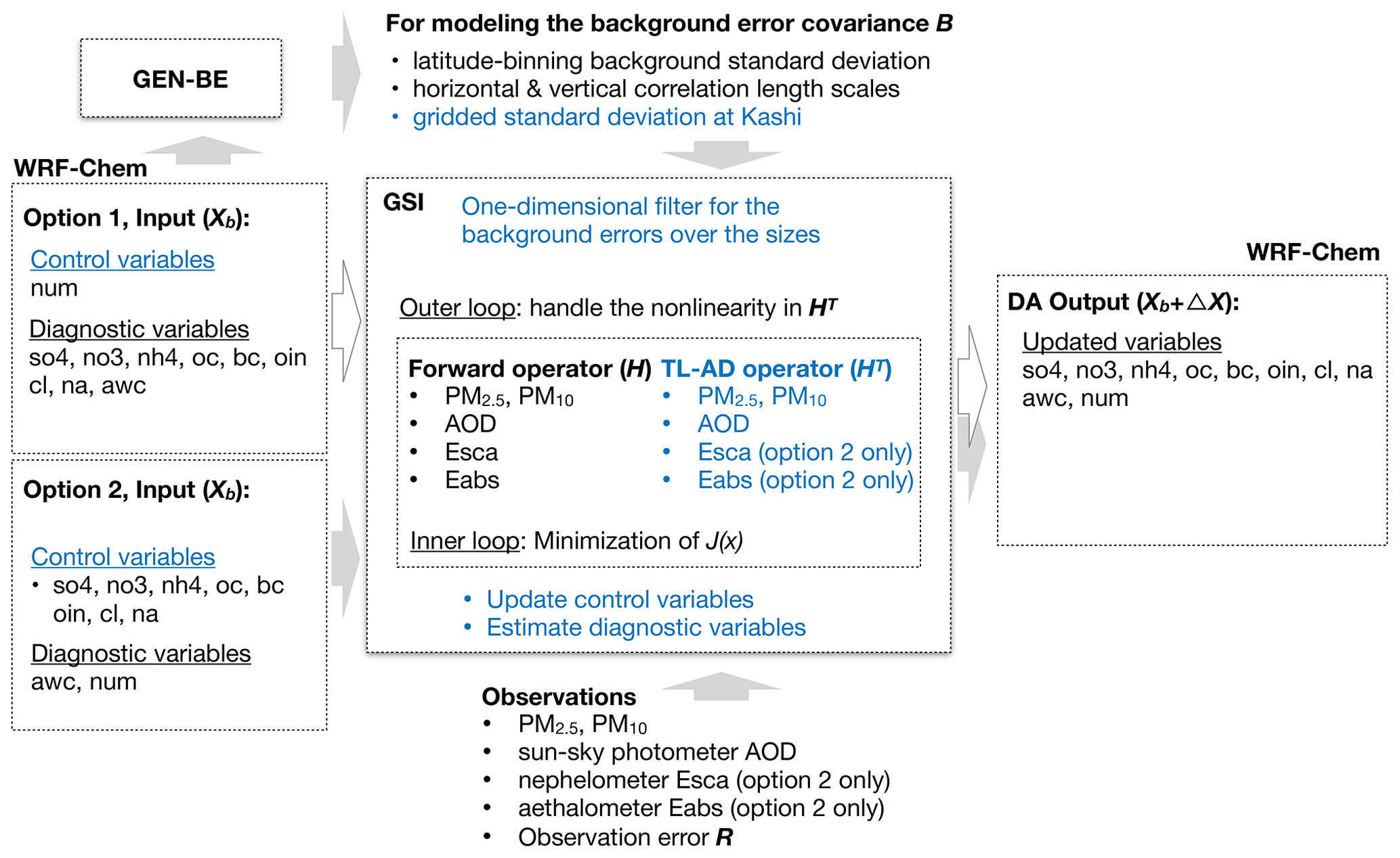
Figure 1 The workflow of aerosol DA in the revised GSI system for the sectional MOSAIC aerosols in WRF-Chem. The contents in blue are the portions we developed. The arrows in gray indicate the workflow of option 2, which was performed in this study to assimilate the aerosol scattering or absorption coefficients. Abbreviations: so4, sulfate; nh4, ammonium; oc, organic carbon; bc, black carbon; oin, other inorganic matter; awc, aerosol water content; num, aerosol number concentration; no3, nitrate; cl, chlorine; na, sodium; Esca, aerosol scattering coefficient; Eabs, aerosol absorption coefficient.

2.2.1 Control variables

The control variables were the mass mixing ratio of each aerosol composition per size bin, which corresponded to the WRF-Chem output data. This set differed from previous studies that lumped aerosols per size bin as control variables (Li et al., 2013; Pagowski et al., 2014). The control variables were six aerosol mass mixing ratios of SO${}_{\mathrm{4}}^{\mathrm{2}-}$, NH${}_{\mathrm{4}}^{+}$, NO${}_{\mathrm{3}}^{-}$, OC, BC, and OIN per size bin, the total of which was 24 for the four size bin simulations. They substantially contributed to the total aerosol mass concentrations. Chlorine and sodium had minuscule background concentrations and remained the background values. In Kashi's case near the desert, the OIN was predominant, accounting for 62 % of PM_2.5 and 82 % of PM₁₀.

Our design of the control variables was different from the AOD assimilation in Saide et al. (2013), with theirs being the natural logarithm of the total mass mixing ratio per size bin, multiplied by the thickness of the model layer. This multiplication of layer thickness prevented many modifications for the high model layers, where aerosols were low in concentrations. The logarithmic transformation decreased the extensive value range in the control variables caused by multiplication. However, since the AOD value is often smaller than 1, their transformation leads to a significant negative logarithm value and an unconstrained DA system. To handle this disadvantage, Saide et al. (2013) introduced two weak constraints in the cost function to cut off the user-defined “extraordinarily high” and “extraordinarily low” concentrations. They repartitioned the total mass per size bin's increments for the composition of each aerosol using the ratio approach. In this study, neither the logarithmic transformation nor the multiplication using layer thickness was set. Our control variable was restricted to the WRF-Chem output variable, and the DA system changed the composition of each aerosol per size bin, depending on the aerosol background errors.

Consistent with Pang et al. (2020), aerosol water content (AWC) was not one of the control variables in our GSI. Otherwise, the AWC might have increased as a mathematical artifact, contrary to the physical constraints imposed by the loading of hydrophilic particles. The AWC was diagnosed in each outer loop according to the analyzed aerosol mass concentration and the background relative humidity, using the WRF-Chem's hygroscopic growth scheme coupled to the revised GSI.

2.2.2 Tangent linear operator for PM_x

The PM₁₀ is the sum of all aerosol dry mass concentrations over the size bins, and the sum of the first three is the PM_2.5 (D. Chen et al., 2019; Wang et al., 2020). The tangent linear operator for PM_x is the gradient of the PM_x concentration to the aerosol chemical mass concentration per size bin:

$$\begin{array}{}\text{(2)}& {\displaystyle \frac{\mathit{\delta }\left[{\mathrm{PM}}_x\right]}{\mathit{\delta }\left[C_{\mathrm{aer},k}\right]}},k=\mathrm{1},\mathrm{\dots },n_{\mathrm{size}},\end{array}$$

where n_size is the number of size bins and is equal to 4 in this study; [.] denotes the mass concentration (µg m⁻³ for PM_x); C_aer,k is the aerosol mass mixing ratio (µg kg⁻¹) of SO${}_{\mathrm{4}}^{\mathrm{2}-}$, NO${}_{\mathrm{3}}^{-}$, NH${}_{\mathrm{4}}^{+}$, OC, BC, and OIN at the kth size bin. Because we did not multiply the chemical mass with a scaling factor to represent some unknown compositions in the summation of PM_x, Eq. (2) always equals 1. It means that we equally distribute the PM_x increment to each aerosol composition per size bin. The PM_2.5 and PM₁₀ are assimilated in the same way. When the observed fine- and coarse-particle concentrations are assimilated simultaneously, we assimilate the concentrations of PM_2.5 and the coarse particulate (PM₁₀-PM_2.5).

2.2.3 Forward operator for aerosol optics in WRF-Chem

We used the original forward operator in WRF-Chem for the aerosol optical parameters (Fast et al., 2006). AOD is calculated as a function of wavelength according to Mie theory. The columnar AOD τ is the sum of layer AOD across the n_z model layers:

$$\begin{array}{}\text{(3)}& \mathit{\tau }=\sum _{z=\mathrm{1}}^{n_z}{\mathit{\tau }}_z=\sum _{z=\mathrm{1}}^{n_z}\sum _{k=\mathrm{1}}^{n_{\mathrm{size}}}{e}_{\mathrm{ext},z,k}\cdot n_{z,k}\cdot H_z,\end{array}$$

where $e_{\mathrm{ext},z,k}$ is the extinction cross section of a single mixing particle in the kth size bin at the zth model layer, n_z,k is the aerosol number concentration, and H_z is the layer thickness. At the surface, the ambient aerosol scattering (E_sca) and absorbing (E_abs) coefficients that are measured by the nephelometer and aethalometer, respectively, are represented as

$$\begin{array}{}\text{(4)}& \begin{array}{rl}& E_{\mathrm{sca}}=\sum _{k=\mathrm{1}}^{n_{\mathrm{size}}}{e}_{\mathrm{sca},\mathrm{1},k}\cdot n_{\mathrm{1},k},\\ & E_{\mathrm{abs}}=\sum _{k=\mathrm{1}}^{n_{\mathrm{size}}}{e}_{\mathrm{abs},\mathrm{1},k}\cdot n_{\mathrm{1},k},\end{array}\end{array}$$

where $e_{\mathrm{sca},\mathrm{1},k}$ and $e_{\mathrm{abs},\mathrm{1},k}$ are the scattering and absorption cross section of a particle at the surface. There is the following relationship:

$$\begin{array}{}\text{(5)}& e_{\mathrm{ext},z,k}=e_{\mathrm{sca},z,k}+e_{\mathrm{abs},z,k}.\end{array}$$

The extinction cross section $e_{\mathrm{ext},z,k}$ of a wet particle with radius $r_{\mathrm{wet},z,k}$ is

$$\begin{array}{}\text{(6)}& e_{\mathrm{ext},z,k}=p_{\mathrm{ext},z,k}\cdot \mathit{\pi }\cdot r_{\mathrm{wet},z,k}^{\mathrm{2}},\end{array}$$

where $p_{\mathrm{ext},z,k}$ is the extinction efficiency, given the desired mixing refractive indexes and the wet particle radius. The $p_{\mathrm{ext},z,k}$ is attained through the Chebyshev polynomial interpolation:

$$\begin{array}{}\text{(7)}& p_{\mathrm{ext},z,k}=\exp \sum _{j=\mathrm{1}}^{n_{\mathrm{coef}}}{c}_{\mathrm{ch}}\left(j\right)\cdot c_{\mathrm{ext},z,k}\left(j\right),\end{array}$$

where c_ch is the coefficient of n_coef order Chebyshev polynomials, $c_{\mathrm{ext},z,k}$ is the polynomial value for the particle's extinction efficiency, which is an internal mixture of all aerosol compositions (i.e., the control variables plus chlorine, sodium, and AWC). The radius is in a logarithmic transform in the AOD subroutine code to handle the broad particle size range from 0.039 to 10 µm. The exponential function in Eq. (7) transforms the logarithm radius back to the normal radius. The aerosol number concentration $n_{z,k,}$ and the aerosol dry (wet) mass concentration $m_{i,z,k}$ have a linkage through the dry (wet) particle radius $r_{\mathrm{dry},z,k}$ ($r_{\mathrm{wet},z,k}$) and the aerosol density ρ_i:

$$\begin{array}{}\text{(8)}& \begin{array}{rl}& n_{z,k}=\sum _i^{n_{\text{wet\_aer}}}{\displaystyle \frac{m_{i,z,k}}{{\mathit{\rho }}_i}}\cdot {\displaystyle \frac{\mathrm{3}}{\mathrm{4}\mathit{\pi }\cdot r_{\mathrm{wet},z,k}^{\mathrm{3}}}}=\\ & \sum _i^{n_{\text{dr\_aer}}}{\displaystyle \frac{m_{i,z,k}}{{\mathit{\rho }}_i}}\cdot {\displaystyle \frac{\mathrm{3}}{\mathrm{4}\mathit{\pi }\cdot r_{\mathrm{dry},z,k}^{\mathrm{3}}}}.\end{array}\end{array}$$

Both the dry and wet particle radius appear in the tangent linear operator. The difference between the second and the third terms in Eq. (8) is whether aerosol water content is counted. n_{wet_aer} is the number of aerosol chemical composition plus aerosol water content ($n_{\text{wet\_aer}}=n_{\text{dr\_aer}}+\mathrm{1}$).

2.2.4 Tangent linear operator developed for AOD

As per the forward operator in Eq. (3) in WRF-Chem, we developed the tangent linear operator for AOD, which requires the derivative of τ in Eq. (3) to the aerosol dry mass concentration (aerosol water content is not a control variable), $m_{i,z,k}$:

$$\begin{array}{}\text{(9)}& \begin{array}{rl}& {\displaystyle \frac{\mathit{\delta }\mathit{\tau }}{\mathit{\delta }{m}_{i,z,k}}}={\displaystyle \frac{\mathit{\delta }{\mathit{\tau }}_z}{\mathit{\delta }{m}_{i,z,k}}}={\displaystyle \frac{\mathit{\delta }{e}_{\mathrm{ext},z,k}\cdot n_{z,k}\cdot H_z}{\mathit{\delta }{m}_{i,z,k}}}\\ & +{\displaystyle \frac{e_{\mathrm{ext},z,k}\cdot \mathit{\delta }{n}_{z,k}\cdot H_z}{\mathit{\delta }{m}_{i,z,k}}}+{\displaystyle \frac{e_{\mathrm{ext},z,k}\cdot n_{z,k}\cdot \mathit{\delta }{H}_z}{\mathit{\delta }{m}_{i,z,k}}}.\end{array}\end{array}$$

The first term on the righthand side of Eq. (9) indicates the change in AOD as the perturbation of extinction cross section. According to Eq. (6), considering that the particle radius is constant, $\mathit{\delta }{e}_{\mathrm{ext},z,k}$ is represented as

$$\begin{array}{}\text{(10)}& \mathit{\delta }{e}_{\mathrm{ext},z,k}=\mathit{\delta }{p}_{\mathrm{ext},z,k}\cdot \mathit{\pi }\cdot r_{\mathrm{wet},z,k}^{\mathrm{2}},\end{array}$$

where δc_ch(j)=0 assuming that the particle radius is constant. This assumption simplifies the tangent linear operator and is also employed in Saide et al. (2013).

Equation (10) is expanded with the derivative of Eq. (7):

$$\begin{array}{}\text{(11)}& \mathit{\delta }{p}_{\mathrm{ext},z,k}=p_{\mathrm{ext},z,k}\cdot \mathit{\left\{}\sum _{j=\mathrm{1}}^{n_{\mathrm{coef}}}{c}_{\mathrm{ch}}\right(j)\cdot \mathit{\delta }{c}_{\mathrm{ext},z,k}(j).\end{array}$$

By expanding $\mathit{\delta }{c}_{\mathrm{ext},z,k}$ in Eq. (11), we have

$$\begin{array}{}\text{(12)}& \begin{array}{rl}& \mathit{\delta }{c}_{\mathrm{ext},z,k}\left(j\right)=\mathit{\delta }{w}_{\mathrm{00}}\cdot C_{\mathrm{ext},\mathrm{00}}\left(j\right)+\mathit{\delta }{w}_{\mathrm{01}}\\ & \cdot C_{\mathrm{ext},\mathrm{01}}\left(j\right)+\mathit{\delta }{w}_{\mathrm{10}}\cdot C_{\mathrm{ext},\mathrm{10}}\left(j\right)+\mathit{\delta }{w}_{\mathrm{11}}\cdot C_{\mathrm{ext},\mathrm{11}}\left(j\right).\end{array}\end{array}$$

The four parameters of C_ext indicate the Chebyshev polynomial values of the extinction efficiencies in the Mie lookup table surrounding the point with the desired mixing refractive indexes and the wet particle radius. The interpolation weights δw are determined as

$$\begin{array}{}\text{(13)}& \begin{array}{rl}& \mathit{\delta }{w}_{\mathrm{00}}=\left(v-\mathrm{1}\right)\mathit{\delta }u+\left(u-\mathrm{1}\right)\mathit{\delta }v,\\ & \mathit{\delta }{w}_{\mathrm{10}}=\left(\mathrm{1}-v\right)\mathit{\delta }u-u\mathit{\delta }v,\\ & \mathit{\delta }{w}_{\mathrm{01}}=\left(\mathrm{1}-u\right)\mathit{\delta }v-v\mathit{\delta }u,\\ & \mathit{\delta }{w}_{\mathrm{11}}=u\mathit{\delta }v+v\mathit{\delta }u,\end{array}\end{array}$$

where

$$\begin{array}{}\text{(14)}& \begin{array}{r}u={\displaystyle \frac{R_{\mathrm{mix}}-R_{\mathrm{low}}}{R_{\mathrm{up}}-R_{\mathrm{low}}}}\mathit{\delta }u={\displaystyle \frac{\mathit{\delta }{R}_{\mathrm{mix}}}{R_{\mathrm{up}}-R_{\mathrm{low}}}},\\ v={\displaystyle \frac{I_{\mathrm{mix}}-I_{\mathrm{low}}}{I_{\mathrm{up}}-I_{\mathrm{low}}}}\mathit{\delta }v={\displaystyle \frac{\mathit{\delta }{I}_{\mathrm{mix}}}{I_{\mathrm{up}}-I_{\mathrm{low}}}}.\end{array}\end{array}$$

In Eq. (14), R_mix and I_mix are the aerosol volume-weighted mean real and imaginary parts of complex refractive indices, respectively. R_up (I_up) and R_low(I_low) are the nearest upper and lower limits for R_mix (I_mix) in the Mie table. Considering $V_{\mathrm{wet},z,k}$ is the volume of all aerosol dry masses plus aerosol water content, the real and imaginary parts and their derivatives are

$$\begin{array}{}\text{(15)}& \begin{array}{rl}& R_{\mathrm{mix},z,k}=\sum _i^{n_{\text{wet\_aer}}}{R}_i\cdot {\displaystyle \frac{m_{i,z,k}}{{\mathit{\rho }}_i\cdot V_{\mathrm{wet},z,k}}},\\ & \mathit{\delta }{R}_{\mathrm{mix},z,k}=\sum _{\mathrm{1}}^{n_{\text{wet\_aer}}}{\displaystyle \frac{R_i}{{\mathit{\rho }}_i\cdot V_{\mathrm{wet},z,k}}}\cdot \mathit{\delta }{m}_{i,z,k},\\ & I_{\mathrm{mix},z,k}=\sum _i^{n_{\text{wet\_aer}}}{I}_i\cdot {\displaystyle \frac{m_{i,z,k}}{{\mathit{\rho }}_i\cdot V_{\mathrm{wet},z,k}}},\\ & \mathit{\delta }{I}_{\mathrm{mix},z,k}=\sum _{\mathrm{1}}^{n_{\text{wet\_aer}}}{\displaystyle \frac{I_i}{{\mathit{\rho }}_i\cdot V_{\mathrm{wet},z,k}}}\cdot \mathit{\delta }{m}_{i,z,k},\end{array}\end{array}$$

where

$$\begin{array}{}\text{(16)}& V_{\mathrm{wet},z,k}=\sum _i^{n_{\text{wet\_aer}}}{\displaystyle \frac{m_{i,z,k}}{{\mathit{\rho }}_i}}.\end{array}$$

Putting Eqs. (12) and (13) into Eq. (11) and assuming the independence of scattering (absorbing) Chebyshev values on the imaginary (real) part leads to

$$\begin{array}{}\text{(17)}& \begin{array}{rl}& \mathit{\delta }{p}_{\mathrm{ext}z,k}=\left[\left(v-\mathrm{1}\right){\mathit{\alpha }}_{\mathrm{sca},\mathrm{00}}+\left(\mathrm{1}-v\right){\mathit{\alpha }}_{\mathrm{sca},\mathrm{10}}\right.\\ & \left.-v{\mathit{\alpha }}_{\mathrm{sca},\mathrm{01}}+v{\mathit{\alpha }}_{\mathrm{sca},\mathrm{11}}\right]\mathit{\delta }u+\\ & \left[\left(u-\mathrm{1}\right){\mathit{\alpha }}_{\mathrm{abs},\mathrm{00}}-u{\mathit{\alpha }}_{\mathrm{abs},\mathrm{10}}+\left(\mathrm{1}-u\right){\mathit{\alpha }}_{\mathrm{abs},\mathrm{01}}\right.\\ & \left.+u{\mathit{\alpha }}_{\mathrm{abs},\mathrm{11}}\right]\mathit{\delta }v,\end{array}\end{array}$$

where

$$\begin{array}{}\text{(18)}& \begin{array}{rl}& {\mathit{\alpha }}_{\mathrm{sca},\mathrm{00}}=p_{\mathrm{sca},\mathrm{1},k}\cdot \sum _{j=\mathrm{1}}^{n_{\mathrm{coef}}}{c}_{\mathrm{ch}}\left(j\right)\cdot C_{\mathrm{sca},\mathrm{00}}\left(j\right),\\ & {\mathit{\alpha }}_{\mathrm{sca},\mathrm{01}}=p_{\mathrm{sca},\mathrm{1},k}\cdot \sum _{j=\mathrm{1}}^{n_{\mathrm{coef}}}{c}_{\mathrm{ch}}\left(j\right)\cdot C_{\mathrm{sca},\mathrm{01}}\left(j\right),\\ & {\mathit{\alpha }}_{\mathrm{sca},\mathrm{10}}=p_{\mathrm{sca},\mathrm{1},k}\cdot \sum _{j=\mathrm{1}}^{n_{\mathrm{coef}}}{c}_{\mathrm{ch}}\left(j\right)\cdot C_{sca,\mathrm{10}}\left(j\right),\\ & {\mathit{\alpha }}_{\mathrm{sca},\mathrm{11}}=p_{\mathrm{sca},\mathrm{1},k}\cdot \sum _{j=\mathrm{1}}^{n_{\mathrm{coef}}}{c}_{\mathrm{ch}}\left(j\right)\cdot C_{\mathrm{sca},\mathrm{11}}\left(j\right),\\ & {\mathit{\alpha }}_{\mathrm{abs},\mathrm{00}}=p_{\mathrm{abs},\mathrm{1},k}\cdot \sum _{j=\mathrm{1}}^{n_{\mathrm{coef}}}{c}_{\mathrm{ch}}\left(j\right)\cdot C_{\mathrm{abs},\mathrm{00}}\left(j\right),\\ & {\mathit{\alpha }}_{\mathrm{abs},\mathrm{01}}=p_{\mathrm{abs},\mathrm{1},k}\cdot \sum _{j=\mathrm{1}}^{n_{\mathrm{coef}}}{c}_{\mathrm{ch}}\left(j\right)\cdot C_{\mathrm{abs},\mathrm{01}}\left(j\right),\\ & {\mathit{\alpha }}_{\mathrm{abs},\mathrm{10}}=p_{\mathrm{abs},\mathrm{1},k}\cdot \sum _{j=\mathrm{1}}^{n_{\mathrm{coef}}}{c}_{\mathrm{ch}}\left(j\right)\cdot C_{\mathrm{abs},\mathrm{10}}\left(j\right),\\ & {\mathit{\alpha }}_{\mathrm{abs},\mathrm{11}}=p_{\mathrm{abs},\mathrm{1},k}\cdot \sum _{j=\mathrm{1}}^{n_{\mathrm{coef}}}{c}_{\mathrm{ch}}\left(j\right)\cdot C_{\mathrm{abs},\mathrm{11}}\left(j\right).\end{array}\end{array}$$

The subscripts of sca and abs in Eqs. (17) and (18) denote “scattering” and “absorption” , respectively. The first term on the righthand side of Eq. (9) is determined using Eqs. (10) and (17). The second term on the righthand side of Eq. (9) indicates the linkage of the aerosol number and mass concentrations. It is the derivative of the dry particle in Eq. (8) by assuming a constant radius:

$$\begin{array}{}\text{(19)}& \mathit{\delta }{n}_{z,k}={\displaystyle \frac{\mathrm{3}\cdot \mathit{\delta }{m}_{i,z,k}}{\mathrm{4}\mathit{\pi }\cdot r_{\mathrm{dyr},z,k}^{\mathrm{3}}\cdot {\mathit{\rho }}_i}}.\end{array}$$

The third term on the righthand side of Eq. (9) contains the layer thickness's derivative to the concentrations in this layer. It indicates that the light attenuation length is based on per unit concentration, which can be intuitively represented by the ratio of layer thickness to the aerosol mass concentration in this layer. Putting Eqs. (10) and (19) into Eq. (9), we have the original formula of the tangent linear operator for AOD for the aerosol dry mass concentration:

$$\begin{array}{}\text{(20)}& \begin{array}{rl}& {\displaystyle \frac{\mathit{\delta }\mathit{\tau }}{\mathit{\delta }{m}_{i,z,k}}}={\displaystyle \frac{\mathit{\delta }{\mathit{\tau }}_z}{\mathit{\delta }{m}_{i,z,k}}}={\displaystyle \frac{\mathit{\delta }{e}_{\mathrm{ext},z,k}\cdot n_{z,k}\cdot H_z}{\mathit{\delta }{m}_{i,z,k}}}\\ & +{\displaystyle \frac{e_{\mathrm{ext},z,k}\cdot \mathit{\delta }{n}_{z,k}\cdot H_z}{\mathit{\delta }{m}_{i,z,k}}}+{\displaystyle \frac{e_{\mathrm{ext},z,k}\cdot n_{z,k}\cdot \mathit{\delta }{H}_z}{\mathit{\delta }{m}_{i,z,k}}}=\\ & [\left(v-\mathrm{1}\right){\mathit{\alpha }}_{\mathrm{sca},\mathrm{00}}+\left(\mathrm{1}-v\right){\mathit{\alpha }}_{\mathrm{sca},\mathrm{10}}-v{\mathit{\alpha }}_{\mathrm{sca},\mathrm{01}}+v{\mathit{\alpha }}_{\mathrm{sca},\mathrm{11}}]\\ & \cdot {\displaystyle \frac{\mathit{\pi }\cdot r_{\mathrm{wet},z,k}^{\mathrm{2}}\cdot R_i\cdot n_{z,k}\cdot H_z}{{\mathit{\rho }}_i\cdot V_{\mathrm{wet},z,k}\cdot \left(R_{\mathrm{up},z,k}-R_{\mathrm{low},z,k}\right)}}+\\ & \left[\left(u-\mathrm{1}\right){\mathit{\alpha }}_{\mathrm{abs},\mathrm{00}}-u{\mathit{\alpha }}_{\mathrm{abs},\mathrm{10}}+\left(\mathrm{1}-u\right){\mathit{\alpha }}_{\mathrm{abs},\mathrm{01}}+u{\mathit{\alpha }}_{\mathrm{abs},\mathrm{11}}\right]\\ & \cdot {\displaystyle \frac{\mathit{\pi }\cdot r_{\mathrm{wet},z,k}^{\mathrm{2}}\cdot I_i\cdot n_{z,k}\cdot H_z}{{\mathit{\rho }}_i\cdot V_{\mathrm{wet},z,k}\cdot \left(I_{\mathrm{up},z,k}-I_{\mathrm{low},z,k}\right)}}+\\ & {\displaystyle \frac{\mathrm{3}{e}_{\mathrm{ext},z,k}\cdot H_z}{\mathrm{4}\mathit{\pi }\cdot r_{\mathrm{dry},z,k}^{\mathrm{3}}\cdot {\mathit{\rho }}_i}}+{\displaystyle \frac{e_{\mathrm{ext},z,k}\cdot n_{z,k}\cdot H_z}{m_{i,z,k}}}\cdot \mathit{\beta },\end{array}\end{array}$$

where β changes the mass unit from µg kg⁻¹ to µg m⁻³. The last righthand term in Eq. (20) may not have a quick convergence in the DA outer loops because the aerosol mass concentration $m_{i,z,k}$ in the denominator often has a low bias, introducing an error into the operator. The error is further amplified by the layer thickness H_z in the numerator. Thus, Eq. (20) cannot lead to a stable analysis. For this reason, we changed the tangent linear operator to account for the columnar mean aerosol extinction coefficient, which is described as follows:

$$\begin{array}{}\text{(21)}& \begin{array}{rl}& {\displaystyle \frac{\mathit{\delta }\stackrel{\mathrm{‾}}{(e_{\mathrm{ext}}\cdot n)}}{\mathit{\delta }{m}_{i,z,k}}}={\displaystyle \frac{H_z}{\sum H_z}}\cdot {\displaystyle \frac{\mathit{\delta }\left(e_{\mathrm{ext},z,k}\cdot n_{z,k}\right)}{\mathit{\delta }{m}_{i,z,k}}}={\displaystyle \frac{H_z}{\sum H_z}}\\ & \cdot [{\displaystyle \frac{\mathit{\delta }{e}_{\mathrm{ext},z,k}\cdot n_{z,k}}{\mathit{\delta }{m}_{i,z,k}}}+{\displaystyle \frac{e_{\mathrm{ext},z,k}\cdot \mathit{\delta }{n}_{z,k}}{\mathit{\delta }{m}_{i,z,k}}}]=\\ & [\left(v-\mathrm{1}\right){\mathit{\alpha }}_{\mathrm{sca},\mathrm{00}}+\left(\mathrm{1}-v\right){\mathit{\alpha }}_{\mathrm{sca},\mathrm{10}}-v{\mathit{\alpha }}_{\mathrm{sca},\mathrm{01}}+v{\mathit{\alpha }}_{\mathrm{sca},\mathrm{11}}]\\ & \cdot {\displaystyle \frac{\mathit{\pi }\cdot r_{\mathrm{wet},z,k}^{\mathrm{2}}\cdot R_i\cdot n_{z,k}}{{\mathit{\rho }}_i\cdot V_{\mathrm{wet},z,k}\cdot \left(R_{\mathrm{up},z,k}-R_{\mathrm{low},z,k}\right)}}+\\ & \left[\left(u-\mathrm{1}\right){\mathit{\alpha }}_{\mathrm{abs},\mathrm{00}}-u{\mathit{\alpha }}_{\mathrm{abs},\mathrm{10}}+\left(\mathrm{1}-u\right){\mathit{\alpha }}_{\mathrm{abs},\mathrm{01}}+u{\mathit{\alpha }}_{\mathrm{abs},\mathrm{11}}\right]\\ & \cdot {\displaystyle \frac{\mathit{\pi }\cdot r_{\mathrm{wet},z,k}^{\mathrm{2}}\cdot I_i\cdot n_{z,k}}{{\mathit{\rho }}_i\cdot V_{\mathrm{wet},z,k}\cdot \left(I_{\mathrm{up},z,k}-I_{\mathrm{low},z,k}\right)}}+\\ & {\displaystyle \frac{\mathrm{3}{e}_{\mathrm{ext},z,k}}{\mathrm{4}\mathit{\pi }\cdot r_{\mathrm{dry},z,k}^{\mathrm{3}}\cdot {\mathit{\rho }}_i}}\cdot \mathit{\beta }\cdot {\displaystyle \frac{H_z}{\sum H_z}}.\end{array}\end{array}$$

In Eq. (21), the operator is based on the extinction coefficient at each layer, weighted by the layer thickness normalized to the total model layer thickness. Correspondingly, the AOD observations and AOD observation error are divided by the total layer thickness at the observation location. Note that the dry ($r_{\mathrm{dry},z,k}$) and wet ($r_{\mathrm{wet},z,k}$) particle radiuses are both present in Eq. (21). Because aerosol water content is not a control variable, $r_{\mathrm{dry},z,k}$ is used in Eq. (19) and appears in Eq. (21). Aerosol water content participates in the computation of internal mixing refractive indexes, and $r_{\mathrm{wet},z,k}$ is also present in Eq. (21). Equation (21) is the final tangent linear operator for AOD DA in this study.

2.2.5 Tangent linear operator developed for surface aerosol attenuation coefficients

The aerosol scattering and absorption coefficients measured by the nephelometer and aethalometer, respectively, are similar to the aerosol extinction coefficient at the surface in Eq. (21). Neither of the two coefficients addresses the layer thickness. The operator for the aerosol scattering coefficient measured by a nephelometer is described as follows:

$$\begin{array}{}\text{(22)}& \begin{array}{rl}& {\displaystyle \frac{\mathit{\delta }(e_{\mathrm{sca},\mathrm{1},k}\cdot n_{\mathrm{1},k})}{\mathit{\delta }{m}_{i,\mathrm{1},k}}}=\mathit{\left\{}\right[\left(v-\mathrm{1}\right){\mathit{\alpha }}_{\mathrm{sca},\mathrm{00}}+\left(\mathrm{1}-v\right){\mathit{\alpha }}_{\mathrm{sca},\mathrm{10}}\\ & -v{\mathit{\alpha }}_{\mathrm{sca},\mathrm{01}}+v{\mathit{\alpha }}_{\mathrm{sca},\mathrm{11}}]\cdot {\displaystyle \frac{\mathit{\pi }\cdot r_{\mathrm{wet},\mathrm{1},k}^{\mathrm{2}}\cdot R_i\cdot n_{\mathrm{1},k}}{{\mathit{\rho }}_i\cdot V_{\mathrm{wet},\mathrm{1},k}\cdot \left(R_{\mathrm{up},\mathrm{1},k}-R_{\mathrm{low},\mathrm{1},k}\right)}}\\ & +{\displaystyle \frac{\mathrm{3}{e}_{\mathrm{sca},\mathrm{1},k}}{\mathrm{4}\mathit{\pi }\cdot r_{\mathrm{dry},\mathrm{1},k}^{\mathrm{3}}\cdot {\mathit{\rho }}_i}}\cdot \mathit{\beta }.\end{array}\end{array}$$

The symbols have the same meaning as before, and the subscript 1 in Eq. (22) denotes the surface layer. The operator for the aerosol absorption coefficient measured by an aethalometer is

$$\begin{array}{}\text{(23)}& \begin{array}{rl}& {\displaystyle \frac{\mathit{\delta }(e_{\mathrm{abs},\mathrm{1},k}\cdot n_{\mathrm{1},k})}{\mathit{\delta }{m}_{i,\mathrm{1},k}}}=\mathit{\left\{}\right[\left(u-\mathrm{1}\right){\mathit{\alpha }}_{\mathrm{abs},\mathrm{00}}-u{\mathit{\alpha }}_{\mathrm{abs},\mathrm{10}}\\ & +(\mathrm{1}-u){\mathit{\alpha }}_{\mathrm{abs},\mathrm{01}}+u{\mathit{\alpha }}_{\mathrm{abs},\mathrm{11}}]\\ & \cdot {\displaystyle \frac{\mathit{\pi }\cdot r_{\mathrm{wet},\mathrm{1},k}^{\mathrm{2}}\cdot I_i\cdot n_{\mathrm{1},k}}{{\mathit{\rho }}_i\cdot V_{\mathrm{wet},\mathrm{1},k}\cdot \left(I_{\mathrm{up},\mathrm{1},k}-I_{\mathrm{low},\mathrm{1},k}\right)}}\\ & +{\displaystyle \frac{\mathrm{3}{e}_{\mathrm{abs},\mathrm{1},k}}{\mathrm{4}\mathit{\pi }\cdot r_{\mathrm{dry},\mathrm{1},k}^{\mathrm{3}}\cdot {\mathit{\rho }}_i}}\cdot \mathit{\beta }.\end{array}\end{array}$$

As shown in the operators, the aerosol mass concentrations' gradients rely on the aerosol number concentration; meanwhile, the number concentration is estimated according to the mass concentration and the particle radius. The two concentrations are intertwined in the DA system, indicating the operator's nonlinearity. This nonlinearity is handled with a succeeding minimization of the cost function within the GSI. The cost function is first minimized with the number concentration in the background field, and the number concentration is updated with the first analyzed aerosol mass concentrations. In the second minimization, the first analysis's number concentration constructs a new operator value, resulting in a new analysis of mass concentrations. This iterative process is denoted as the “outer loop”, which is repeated several times to attain the final analysis (Massart et al., 2010). We set 10 maximum iterations in the experiments. The cost function in most analyses reaches the minimum in two or three outer loops. The WRF-Chem AOD code is coupled to the GSI subroutine at the place of invoking CRTM. The tangent linear operators of Eqs. (21), (22), and (23) are simultaneously determined in the subroutines, which are cyclically invoked in the outer loops.

2.2.6 Aerosol complex refractive indexes in GSI

Table S1 in the Supplement shows the complex refractive indexes for each aerosol chemical composition in the revised GSI. The refractive indexes are for 11 wavelengths, including 4 for CE318, 3 for the nephelometer, 3 for the aethalometer, and 1 for 550 nm MODIS AOD (not assimilated in this study). The real parts of refractive indexes of sulfate, nitrate, and ammonium are similar and refer to Toon et al.'s (1976) data. The real part is 1.53 at 440 nm and decreases to 1.52 at 1020 nm. The refractive indexes of OC and BC are constant across the wavelengths, being 1.55–0.001i for OC (Chen and Bond, 2010) and 1.95–0.79i for BC (Bond and Berstrom, 2006). The dust refractive index's real part is a constant value of 1.54 (Zhao et al., 2010). The dust refractive index's imaginary part depends on the dust mineralogy, size distribution, and shape associated with the dust sources. Cheng et al. (2006) reported the desert dust refractive index in winter and spring at Dunhuang, a city adjacent to the Taklimakan desert's northeast side. Their imaginary part value was approximately in the ranges of 0.0008 to 0.0028 at 440 nm, 0.0006 to 0.0030 at 670 nm, 0.0005 to 0.0036 at 870 nm, and 0.0005 to 0.0040 at 1020 nm (see Fig. 9 in their paper). Di Biagio et al. (2019) retrieved the dust's imaginary part in the Taklimakan desert's north edge (41.83^∘ N, 85.88^∘ E). Their dust imaginary part decreased from 0.0018 ± 0.0008 at 370 nm to 0.0005 ± 0.0002 at 950 nm, much lower than the generic values in climate models. The imaginary part's retrieval uncertainty is related to the iron oxide in dust samples, the cutoff coarse-particle size (< 10 µm in Di Biagio et al., 2019), and the spherical particle assumption applied in the retrieval algorithm. Here, we admit the high uncertainty and use the imaginary part following the generic model values (Table S1 in the Supplement), which are higher than the upper data limits of Di Biagio et al. (2019) and are close to the values of Cheng et al. (2006). The desert dust has a stronger absorption at shortwave wavelengths. The refractive index of a wavelength without exact literature data uses the nearby wavelength's data in the literature. Aerosol density is necessitated to compute aerosol optical parameters in the AOD forward operator and construct our tangent linear operator. The Supplement also shows the aerosol density (Table S2) that follows the data in Barnard et al. (2010).

2.3 Background error covariance (BEC)

Many aerosol DA studies used the National Meteorological Center (NMC) method (Parrish and Derber, 1992) to model the BEC matrix. The NMC method uses long-term archived weather data created in forecast cycles. It computes the statistical differences between two forecasts with different leading lengths (e.g., 24 and 48 h) but which are valid at the same time. The NMC method is workable because solving global weather forecasts is an initial value problem of mathematical physics. A slight difference in the initial atmospheric state would lead to a substantially different prediction because of the chaos in the atmosphere. However, a regional model is a boundary value problem (Giorgi and Mearns, 1999). As the regional model runs, the influence of the initial conditions becomes weak, while lateral boundary conditions always take effect. The reanalysis data that drive the paring regional model simulations are similar and lead to a limited difference between the paring simulations. The NMC method's BEC would therefore underestimate the aerosol error in WRF-Chem. Kumar et al. (2019) assimilated AOD in the contiguous United States based on the NMC method's BEC. They perturbed the background emissions by adding the gridded mean differences of four emission inventories. Their BEC accounting for meteorology and emissions uncertainties reduced the AOD bias by 38 %, superior to 10 % bias reduction, counting the meteorology uncertainty alone.

Some aerosol DA studies have created background error variance using the ensemble simulations by randomly disturbing model lateral boundary conditions and surface emissions (Peng et al., 2017; Ma et al., 2020). The ensemble experiments represent the model error better but significantly increase the computational burden. Here, we used the variance of the background hourly aerosol concentrations in April to represent the background error variance. The rationale of this approach is that the Tarim Basin acts as a “dust reservoir” and traps dust particles for a period before the dust is carried long-distance by wind (Fan et al., 2020). The model bias in dust concentration is correlated with aerosol concentration variation as the weather fluctuates. The model bias is small on clear days when the aerosol concentration is low. The bias is large when the concentration is high on heavily polluted days. The mean aerosol concentration correlated positively with the aerosol variation. Using aerosol concentration variance to represent the aerosol error prioritizes DA modification of aerosols having high background mean concentrations. It was similar to the way in Sič et al. (2016), which set a percentage of the first guess field for the background error variance.

We calculated the background error statistics, including the aerosol standard deviation and the horizontal and vertical correlation length scales, using the GENerate the Background Errors (GEN-BE) software (Descombes et al., 2015), based on the 1-month hourly aerosol concentrations in WRF-Chem. We obtained the statistics of four static BECs for the four DA analysis hours (i.e., 00:00, 06:00, 12:00, and 18:00 UTC), respectively. The DA procedures for the four analysis times a day in April 2019 repeatedly use the background error statistics at the corresponding analysis time.

A usual strategy to enrich the samples of model results for the error statistics is to gather model grid points with similar atmosphere characteristics, referred to as “binning.” The statistics are spatially averaged over the binned grid points. The GEN_BE default strategy for GSI is latitude binning, which creates a latitude-dependent error correlation function (Fig. 2a). The latitude binning is generally used for latitude flow dependency and works for large and global domains (Wu et al., 2002). However, we found that using the latitude-binning strategy overestimated the PM_x concentration when assimilating aerosol optical observations. One reason for this overestimation was related to the model's low bias in particle extinction efficiency, as discussed in Sect. 3.3. Another plausible reason is related to the background model error's vertical profile. The maximum dust error in the desert occurred at the surface (Fig. 2e) because of the local dust emissions, while the maximum error at Kashi was at the dust transporting layer above the surface (Fig. 2d). Owing to the Taklimakan Desert's vast extent, the latitude binning suppressed the local error characteristics at Kashi and led to a vertical error profile (Fig. 2c) similar to that over the desert (Fig. 2e).

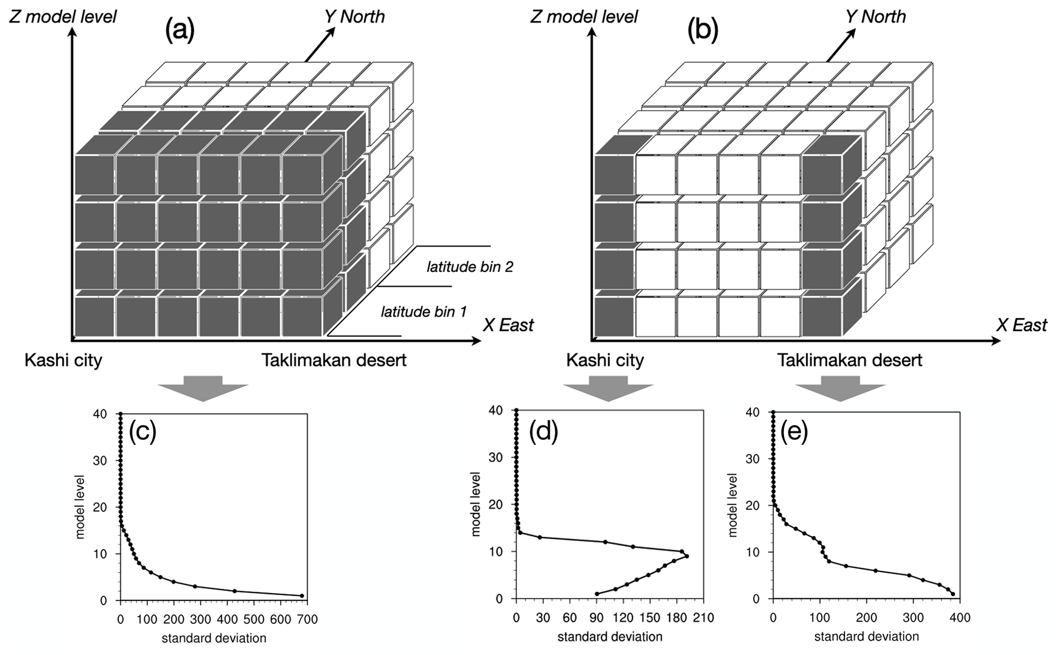
Figure 2 Schematic diagram of the binning strategy for modeling background error covariance matrix on (a) the latitude-binning data or (b) the gridded data; and the vertical profiles of standard deviations (µg kg⁻¹) of the fourth size bin OIN component concentration at 06:00 UTC over a few mild dust episodes in April 2019 (c) on average over the latitude bins, (d) at Kashi city grid, and (e) at the Taklimakan desert grid (i.e., 1.5^∘ east of Kashi city).

For this reason, we used the standard deviation of the control variable at each model grid to replace the latitude-binning standard deviation. The horizontal and vertical correlation length scales were calculated based on the latitude-binning data. Figure 3 shows the background error statistics generated by the GEN_BE software, which provided the input to the GSI. The OIN component showed high background errors in the third and fourth particle sizes at the transporting layer above the surface (Fig. 3f). The aerosol compositions related to anthropogenic emissions (i.e., sulfate, nitrate, ammonium, OC, and BC, referred to here as “anthropogenic aerosols”) that had maximum errors in the second particle size, with the greatest vertical error at the surface. The background error for OIN composition was a factor of 2–3 higher than that for anthropogenic aerosols because of the high background dust concentration.

Figure 3 Background error standard deviations at Kashi grid (std, a–f, µg kg⁻¹), horizontal correlation length scales (hls, g–l, km), and vertical correlation length scales (vls, m–r, km) at 00:00 UTC in April 2019 for the sectional sulfate (SO₄), nitrate (NO3), ammonium (NH4), organic aerosol (OC), black carbon (BC), and other inorganic aerosols (OIN, including dust) in model domain 2. The horizontal and vertical correlation length were computed based on the latitude bins with a half degree width.

The horizontal and vertical correlation length scales determine the range of observation innovations spreading from the observation locations. The horizontal influences had small changes in altitude within the lowest 15 model layers (below a height of ∼ 5 km above ground), indicating that the dust transport layer was well-mixed in the lower atmosphere. This deep dust layer was consistent with Meng et al. (2019). They showed that the dust in spring was vertically mixed in a thick boundary layer to a height of 3–5 km in the Tarim Basin. The vertical correlation length scales first increased from low values at the surface to high values at ∼ 2.5 km in height (for the eight to nine layers), indicating upward aerosol flux in windy days. The vertical correlation length scale quickly decreased from the maximum value with a further altitude rise. The maximum correlation length above the ground indicates a laminar air motion during the dust storm.

Because the background model error per size bin is independent, the DA modification of an aerosol concentration would be quite large in a single size bin with the maximum background error (e.g., the OIN in the fourth particle size). To avoid the excessive accumulation of increment, we added a one-dimensional recursive filter for the background covariances of control variables across the size bins, with a correlation length scale of four bin units.

2.4 Observational data and errors

The Dust Aerosol Observation–Kashi field campaign was performed at Kashi from 00:00 UTC 25 March to 00:00 UTC 1 May 2019. The site was located at the Kashi campus of the Aerospace Information Research Institute, Chinese Academy of Sciences (39.50^∘ N, 75.93^∘ E; Li et al., 2018), about 4 km northwest of Kashi city. The site aerosol observations included (1) the multi-wavelength AOD measured by the sun–sky photometer (Cimel CE318); (2) the multi-wavelength aerosol scattering and absorption coefficients at the surface, measured with a nephelometer (Aurora 3000) and aethalometer (Magee AE-33), respectively; and (3) the hourly PM_2.5 and PM₁₀ observations, measured with a METONE BAM-1020 continuous particulate monitor. All the instruments were deployed at the roof of a three-story building on the campus. Please refer to Li et al. (2020) for more details about the field campaign.

Table 1 summarizes the observation periods, the aerosol optical data's wavelengths, and the observation errors. The multi-wavelength data of each type of optical observation were assimilated simultaneously. The observation errors of PM_x are handled in the conventional way (Schwartz et al., 2012; Chen et al., 2019), which contains the measurement error (e₁) and the representation error (e₂). The measurement error is the sum of a baseline error of 1.5 µg m⁻³ and 0.75 % of the observed PM_x concentration. The representation error is the measurement error multiplied by the half-squared ratio of the grid spacing to the scale distance. The scale distance denotes the site representation in GSI and has four default values of 2, 3, 4, and 10 km, corresponding to the urban, unknown, suburban, and rural sites. We used 3 km for the scale distance in this study. As we had a single site in Kashi, it is difficult to estimate the site representation error. Since the DA analysis was based on the inner model domain with a horizontal resolution of 5 km, close to the site distance to the Kashi urban area, we assumed the aerosol optical measurement had good representativeness of the model grid. The observation error of CE318 AOD took the AERONET AOD uncertainty of 0.01 in cloud-free conditions (Holben et al., 1998). The AOD observational error was further divided by the total model layer thickness in GSI. It is difficult to determine instrumental errors in nephelometers and aethalometers, and we set their instrumental errors to 10 Mm⁻¹, equivalent to the magnitude of the Rayleigh extinction coefficient. The observational errors were uncorrelated, with R being a diagonal matrix.

Table 1 The observed surface particle concentration, aerosol scattering coefficient (Esca), aerosol absorption coefficient (Eabs), and AOD used for the DA analysis and their observational errors.

2.5 Experimental design

The WRF-Chem simulations were configured in a two-nested domain centered at 41.5 ^∘ N, 82.9 ^∘ E. The coarse domain was a 120 × 100 (west–east  × north–south) grid with a horizontal resolution of 20 km covering the Taklimakan Desert, and the fine domain was an 81 × 61 grid with a resolution of 5 km, focusing on Kashi and environs (Fig. 4a). Both domains had 41 vertical levels extending from the surface to 50 hPa. The lowest model layer at the site was approximately 25 m height from the ground. The two domains were two-way coupled. The coarse domain covered the entire dust emission source, providing dust transport fluxes at the fine domain's lateral boundaries. The aerosol radiative effect was set to provide feedback on the meteorology. The indirect effect of aerosols was not set in the experiments. Initial and lateral boundary meteorological conditions for WRF-Chem were the 1^∘ resolution of the National Centers for Environmental Prediction Final Analysis data created by the Global Forecast System model. The meteorological lateral boundary conditions for the coarse domain were updated every 6 h and were linearly interpolated between the updates in WRF-Chem. We did not set the chemical boundary conditions for the coarse domain. The Multiresolution Emission Inventory of China (MEIC) for 2010 (http://www.meicmodel.org, last access: March 2021) provided anthropogenic emission levels. The yearly emission differences in 2010–2019 may bias the aerosol chemical simulation, but this bias is hard to quantify due to a lack of aerosol chemical observations in this city. As the significant pollutant at Kashi is dust, we just ignore the model uncertainties due to the yearly differences in anthropogenic emission inventories. The biogenic emission levels were estimated online using the Model of Emissions of Gases and Aerosols from Nature (Guenther et al., 2006). Wildfire emissions were not set in the experiments.

Figure 4 Topography in China (a) and the model domains with the grid resolution of 20 km (b) and 5 km (c) in WRF-Chem.

We conducted a 1-month WRF-Chem simulation for April 2019, starting at 00:00 UTC on 27 March and discarding the first 5 d for spin-up. The revised GSI system modified the aerosols in the fine domain at 00:00, 06:00, 12:00, and 18:00 UTC each day starting from 00:00 UTC 1 April until the end of the month. We assimilated the observations four times a day because the reanalyzed meteorological data were available for the four time slices, facilitating the model restarting from the DA analyses. The hourly PM_x observations were assimilated at the exact time of analysis. The observed AOD and aerosol scattering or absorption coefficients were assimilated when they fell within 3 h before the time of analysis. Table 2 shows the DA experiments, in which the multi-wavelength AOD (440, 675, 870, and 1020 nm) in DA_AOD, the aerosol scattering coefficients (450, 525, and 635 nm) in DA_Esca, and the aerosol absorption coefficients (470, 520, and 660 nm) in DA_Eabs were assimilated simultaneously in each experiment. The literal meanings of the experimental names denote the observations that were assimilated. To study the impact of DA on aerosol direct radiative forcing (ADRF), we modified the WRF-Chem code to calculate the shortwave irradiance with and without aerosols at each model integration step. The modified WRF-Chem model restarted from each DA analysis and ran to the next analysis time. Each running performed the radiation transfer calculation twice, and each calculation saw the aerosols and clean air, respectively. The irradiance difference between the two pairing calls was aerosol radiative forcing. Section 4.2 shows the DA effects on the clear-sky ADRF values.

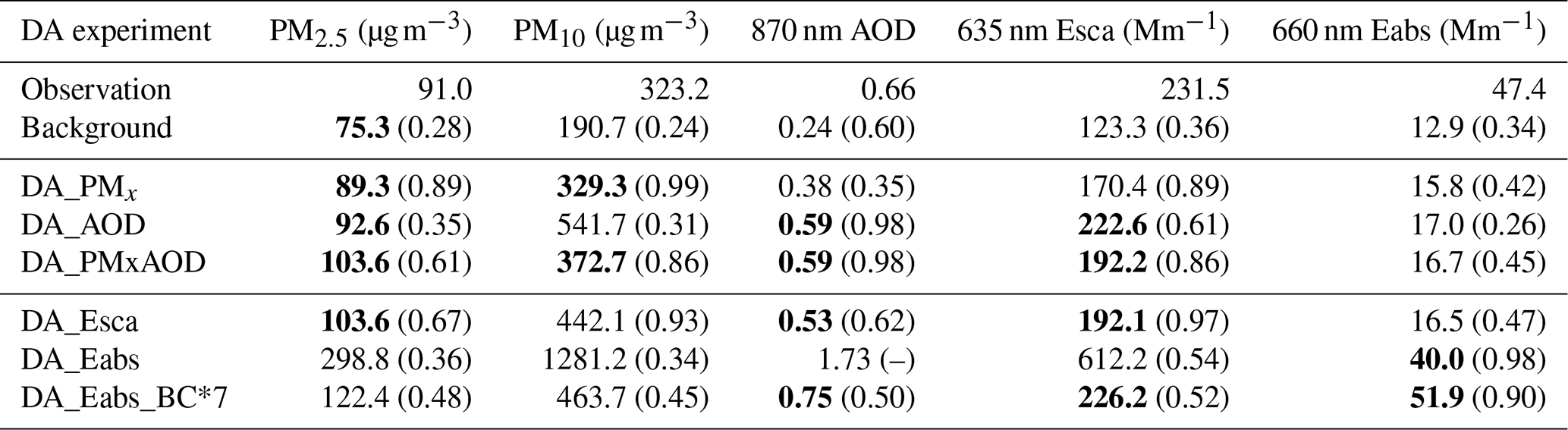
Table 2 The mean values of the PM_2.5 and PM₁₀ concentrations (µg m⁻³), 635 nm aerosol scattering coefficient (Esca, Mm⁻¹), 660 nm aerosol absorption coefficient (Eabs, Mm⁻¹), and 870 nm AOD in the background and analysis data and their correlation coefficients (in brackets) with the observations at 00:00, 06:00, 12:00, and 18:00 UTC at Kashi in April 2019. The bold numbers denote the mean value that is not significantly different from the observation, and the line (–)denotes an insignificant correlation. Both the statistical tests of the mean difference and correlation are conducted at the significance level of 0.05.

3 Results

3.1 Evaluation of control experiment

Table 2 shows the monthly mean values and correlations between the observed data and the model results. The statistical values were based on the pairing data between the model results and the observations. Figure 6 show the surface PM_x concentrations, aerosol scattering coefficients, and AOD when assimilating the observations at 00:00, 06:00, 12:00, and 18:00 UTC each day in April.

Figure 5 Monthly mean PM₁₀ concentration (µg m⁻³) and the streamlines of the 10 m wind (m s⁻¹) in April (a, b) and their daily mean anomalies (c, d) during a dust storm on 24 April to the monthly mean values. Only the streamlines at the topographical height lower than 2500 m are shown for clarity. The rectangles in panels (b) and (d) denote the fine model domain 2, which was the geographical range in panels (a) and (c). The black points indicate Kashi city.

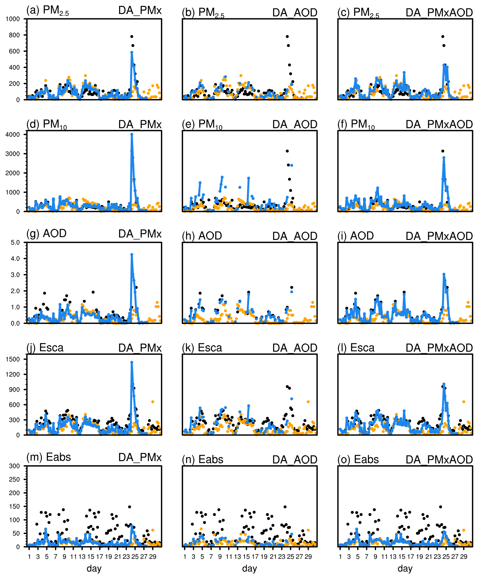
Figure 6 Comparison of PM_2.5 (µg m⁻³; a–c), PM₁₀ (µg m⁻³; d–f), 870 nm AOD (g–i), 635 nm aerosol scattering coefficient (Esca, Mm⁻¹; j–l), and 660 nm aerosol absorption coefficient (Eabs, Mm⁻¹; m–o) in the observation (black solid points), the background simulation (orange solid points), and the DA analyses (blue line) when assimilating the observed PM_2.5 and PM₁₀ (DA_PM_x), AOD (DA_AOD), and simultaneously assimilating PM_x and AOD (DA_PMxAOD) at Kashi in April 2019.

Kashi is in the junction between the Tian Shan to the west and the Taklimakan Desert to the east (Fig. 5a). In the Tarim Basin, the prevailing surface wind is easterly or northeasterly, which raises dust levels and carries the particles westward (Fig. 5b). An intense dust storm hit the city at noon on 24 April 2019, with a peak PM₁₀ concentration exceeding 3000 µg m⁻³. The dust storm traveled across the northern part of the desert and carried the dust particles to Kashi and the mountainous area (Fig. 5c, d). A few mild dust storms occurred at Kashi on 3–5, 8–11, and 14–17 April, and the maximum PM₁₀ concentrations were in the range of 400–600 µg m⁻³. The time series of PM_2.5, aerosol scattering or absorption coefficient, and AOD showed patterns similar to those for PM₁₀ (Fig. 6).

WRF-Chem captured the main dust episodes but significantly underestimated the aerosols at Kashi (Table 2). The monthly mean background concentrations of PM_2.5 and PM₁₀ were 17 % and 41 % lower than the observed values, respectively, with a low correlation (R < 0.3). The simulated dust storm on 24 April was a mild dust event and had a maximum PM₁₀ of ∼ 300 µg m⁻³, 1/10 of the observed value. The model underestimates the aerosol scattering or absorption coefficients and AOD by 40 %–70 %.

The OIN component accounted for the model bias in PM₁₀ on dusty days. Zhao et al. (2020) proposed that the GOCART scheme reproduced dust emission fluxes under weak wind erosion conditions but underestimated the emissions in conditions of strong wind erosion. We did not assimilate meteorology. The model bias in the surface wind could introduce an error in dust emission and a bias in the number of dust particles entering the city. In the non-dust days with the PM₁₀ lower than the 25th percentile PM₁₀ in April, the model PM_2.5 on average accounted for 60 % of the observed data levels. The PM_2.5 low bias could be due to the lack of SOA chemistry in our experiments and the low emission bias in the residential sector, a major source of anthropogenic emissions for PM_2.5, BC, and OC in the developing western area. The residential sector accounts for 36 %–82 % of the primary particle emissions, according to the MEIC emission inventory (Li et al., 2017), and is the primary source of uncertainty in anthropogenic emissions inventories in China.

3.2 Assimilating PM_2.5 and PM₁₀ concentrations

Simultaneous assimilation of the observed PM_x (DA_PM_x) improved both the fine- and coarse-particle concentrations, with a substantial increase in the third and fourth particle sizes of the OIN composition (Fig. 8f). The analyzed monthly mean PM₁₀ increased to 329.3 µg m⁻³, with a high correlation of 0.99. The analyzed monthly mean PM_2.5 was improved to 89.3 µg m⁻³, although it was still lower than the observed levels, with a high correlation of 0.89. The low bias in PM_2.5 and the high bias in PM₁₀ in the analyses were mainly in the dust storm on 24–25 April (Fig. 6a, d).

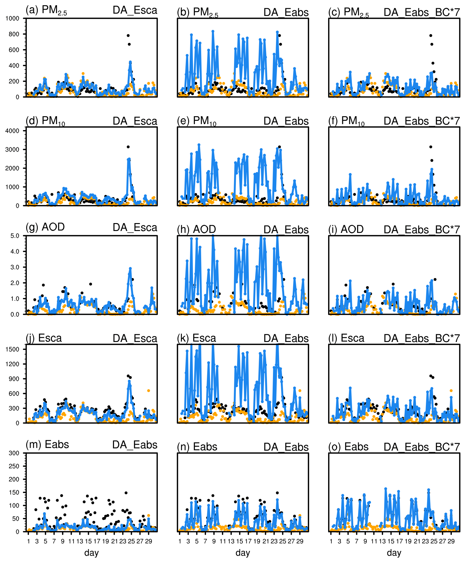
Figure 7 Comparison of PM_2.5 (µg m⁻³; a–c), PM₁₀ (µg m⁻³; d–f), 870 nm AOD (g–i), 635 nm aerosol scattering coefficient (Esca, Mm⁻¹; j–l), and 660 nm aerosol absorption coefficient (Eabs, Mm⁻¹; m–o) in the observation (black solid points), the background simulation (orange solid points), and the DA analyses (blue line) when assimilating the aerosol scattering coefficient (DA_Esca), aerosol absorption coefficient (DA_Eabs), and absorption coefficient with the background error of BC enlarged by a factor of 7 (DA_Eabs_BC*7) at Kashi in April 2019.

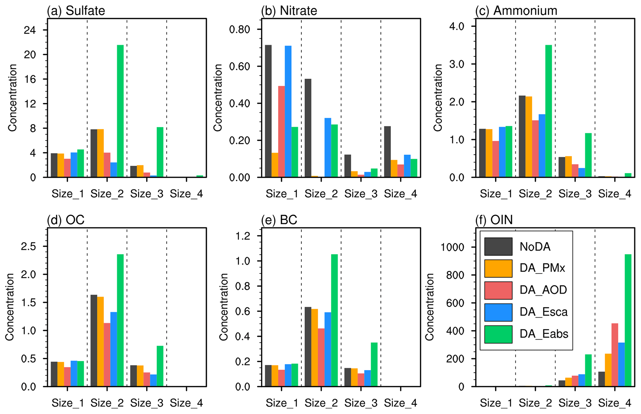
Figure 8 Mean aerosol concentrations (µg m⁻³) per size bin in the background (NoDA) and the DA analyses when assimilating each individual observation at Kashi in April 2019.

Applying the inter-size bin correlation length caused the interlinked analyses of PM_2.5 and PM₁₀. In the desert area, the coarse and fine dust is readily affected by BEC's magnitude of the fourth size bin OIN (oin_a04). We performed a few sensitivity tests decreasing the BEC of oin_a04 by 10 % each time until the BEC was 30 % of its original value. The magnitude of 30 % of oin_a04 was comparable to the magnitude of the third size bin (oin_a03) OIN's background error. As shown in Table S3, because the oin_a04's BEC reduction relaxes the constraint on the coarse particle, the PM₁₀ bias becomes more negative along with the decrease in on_a04's BEC. The PM_2.5 bias meanwhile becomes more positive. Correspondingly, the ratio of PM_2.5 to PM₁₀ was increased to 0.33 with 30 % of oin_a04's BEC, higher than the observed value of 0.28. According to these experiments, the original BEC of oin_a04 is a reasonable tradeoff. The inter-size bin correlation length tunes the cross size bin modifications and also affects the analyses of PM_2.5 and PM₁₀. The experiment's correlation length is a little bit arbitrary, but we found that our DA analyses were not very sensitive to the inter-size bin correlation length.

According to our BEC modeling strategy, the DA system preferentially modified the coarse-particle concentrations because of the coarse particles' high background model error. Intuitionally, our modification that mainly focused on the highest concentration of coarse particles was reasonable. It decreased the model biases by raising the heaviest aerosol loadings. As a result, the ratio of PM_2.5 to PM₁₀ decreased from 0.39 in the background to 0.27 in DA_PM_x, approaching the observed ratio of 0.28. Such improvement was consistent with the correction required for the model desert dust in literature. Kok et al. (2011) found that regional and global circulation models underestimate the fraction of emitted coast dust ($>\sim$ 5 µm) and overestimate the fraction of fine dust (< 2 µm diameter). Adebiyi and Kok (2020) claimed that too rapid a deposition of coarse dust out of the atmosphere accounts for the missing coarse dust in models. According to Kashi's AOD between 440 nm and 1020 nm, the observed Ångström exponent (AE) was 0.18, while the background value was 0.54 (Table 3), showing too many fine particles in the background field. DA_PM_x reduced the AE value to 0.30, a small improvement but not sufficient.

As the particle concentration increased, the 635 nm aerosol scattering coefficient in DA_PM_x moderately increased to 170.4 Mm⁻¹, still lower than the observed level of 231.5 Mm⁻¹, with a high correlation of 0.89. The scattering AE was 1.32 in the background and decreased to 0.96 (Table 3), indicating a more reasonable wavelength dependence of the coarse particles' scattering in the analysis. The analyzed 660 nm absorption coefficient had a small improvement, which was 15.8 Mm⁻¹, 67 % lower than observed levels, with a correlation of 0.42. There was no improvement in absorption AE, which increased to 1.84 in DA_PM_x, far higher than the observation value of 1.65. The analyzed 870 nm AOD showed a monthly mean value of 0.38 in DA_PM_x, 42 % lower than observed levels, with a low correlation of 0.35.

Figure 9a shows the diurnal concentrations of PM₁₀ in the analyses in April. The observed PM₁₀ showed a substantial variation at 18:00 UTC, the local midnight. This substantial nocturnal variation was partly owing to the dust storm that started on 24 April and ended the next day. This midnight variation was also related to a nocturnal low-level jet. Ge et al. (2016) pointed out a nocturnal low-level jet at the height of 100–400 m, with a wind speed of 4–10 m s⁻¹ throughout the year in the Tarim Basin. They stressed that the low-level jet broke down in the morning, transporting its momentum toward the surface, and increased dust emissions. The nocturnal low-level jet increased the possibility of dust particles moving towards the city at night, causing a high PM₁₀ variation at 18:00 UTC. The diurnal changes in the DA analyses followed the observed levels but had higher mean values.

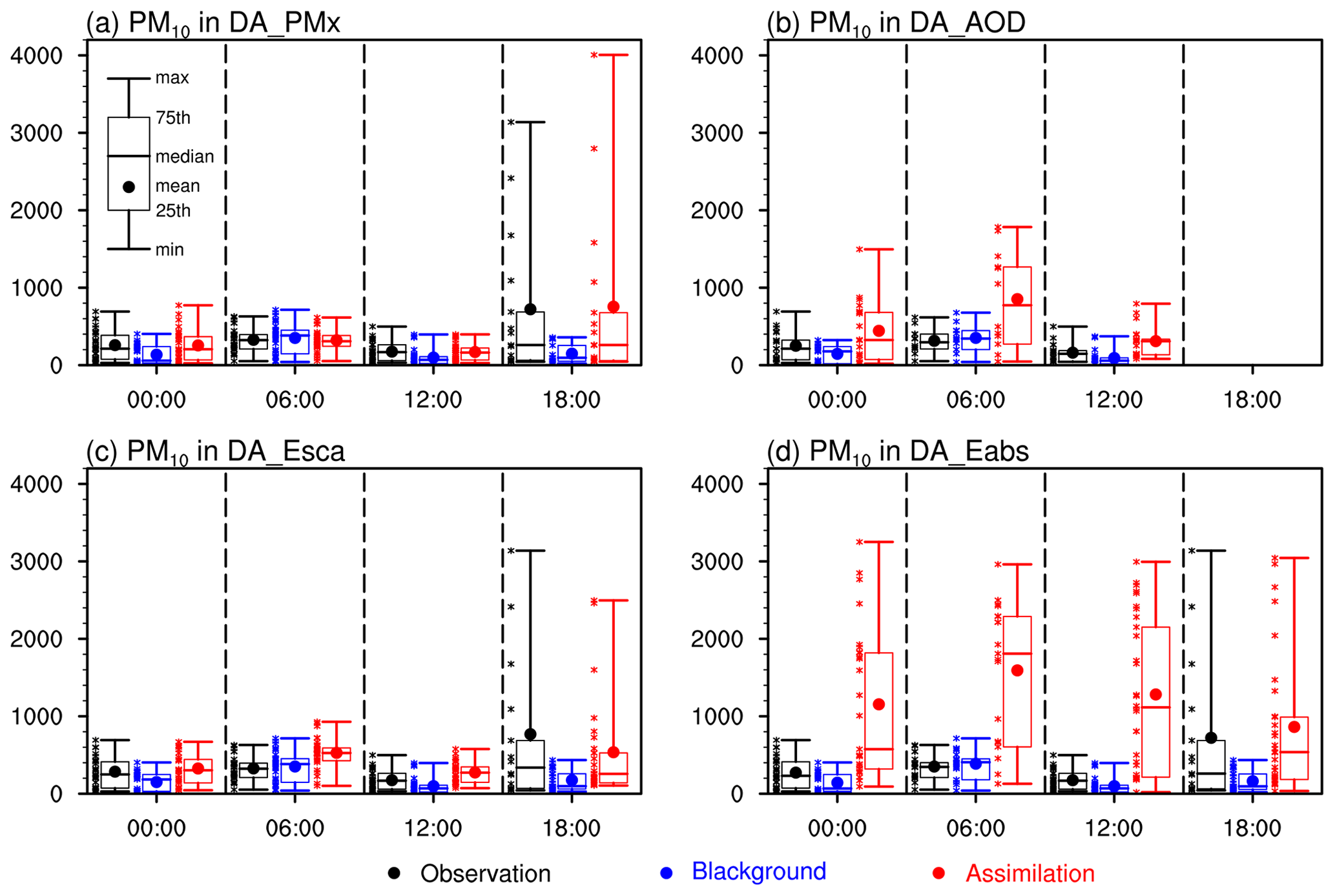
Figure 9 Surface PM₁₀ concentrations (µg m⁻³) in the observation (black), background simulation (blue), and the DA analyses (red) at 00:00, 06:00, 12:00, and 18:00 UTC in April 2019 when assimilating the observations of (a) PM_x, (b) AOD, (c) aerosol scattering coefficients (Esca), and (d) aerosol absorption coefficient (Eabs), respectively. The DA_AOD had no analysis at 18:00 UTC that was local midnight. Kashi is 6 h ahead of UTC (UTC+6).

3.3 Assimilating AOD

Assimilating AOD (DA_AOD) improved the monthly mean of 870 nm AOD to 0.59, approaching the observed value of 0.66, with a high correlation of 0.98 (Fig. 6h). The monthly mean PM_2.5 was improved to 92.6 µg m⁻³, quite close to the observed level of 91 µg m⁻³, but the analyzed PM₁₀ was 541.7 µg m⁻³, 68 % higher than the observed value. The DA system improved the AOD at the price of deteriorating the data quality of surface coarse-particle concentrations. Such surface particle overestimations have been reported in previous studies (Liu et al., 2011; Ma et al., 2020; Saide et al., 2020). As a result, the ratio of PM_2.5 to PM₁₀ reduced to 0.17 in DA_AOD, which was too far compared with the observed ratio of 0.28. The overestimation of aerosol mass concentration also tended to raise scattering or absorption coefficients. The analyzed 635 nm scattering coefficient in DA_AOD increased to 222.6 Mm⁻¹, slightly lower than the observed value. The analyzed 660 nm absorption coefficient slightly increased to 17.0 Mm⁻¹, 64 % lower than the observed value.

The scattering and absorption AE values in DA_AOD had the responses as those in DA_PM_x. As shown in Table 3, the scattering AE decreased to 0.44 in DA_AOD, which was slightly better than the AE value of 0.96 in DA_PM_x. By contrast, the absorption AE increased to 1.97 in DA_AOD, deviating greatly from the observed value. The analysis fit to the aerosol scattering overwhelmed the fit to the aerosol absorption. The AE based on AOD was reduced to −0.01 in DA_AOD, in line with the decrease in DA_PM_x, but the reduction in DA_AOD was much lower than the observation value of 0.18.

Table 4 shows the ratios of the AOD and aerosol scattering or absorption coefficients to the surface PM₁₀ concentrations. The ratio of AOD to PM₁₀ in the background model result was one-third of the observed levels. The observed mass scattering coefficient (Esca $/$ PM₁₀) was 1.05 Mm⁻¹ µg⁻¹ m³, while the background value was only 0.65 Mm⁻¹ µg⁻¹ m³. DA_AOD did not eliminate the low bias but lowered the ratio to 0.51 Mm⁻¹ µg⁻¹ m³. The same thing occurred for Eabs $/$ PM₁₀, which was 0.09 in the background and 0.05 in DA_AOD, much lower than the observed value of 0.25. Figure 10 shows these mean ratios at the other wavelengths. The low bias in AOD $/$ PM₁₀ was comparable at each wavelength with a slightly stronger low bias in short wavelengths (Fig. 10a). The ratios' low biases indicated the low scattering and absorption efficiencies, and the DA system overestimated the PM₁₀ to fit the observed AOD data.

Table 3 The Ångström exponent values based on the AOD (440 and 1020 nm; AEaod), aerosol scattering coefficients (450 and 635 nm; AEsca), aerosol absorption coefficients (470 and 660 nm; AEabs), and the surface single-scattering albedo (SSA_srf = Esca525$/$(Esca525+Eabs520)) at Kashi in April 2019.

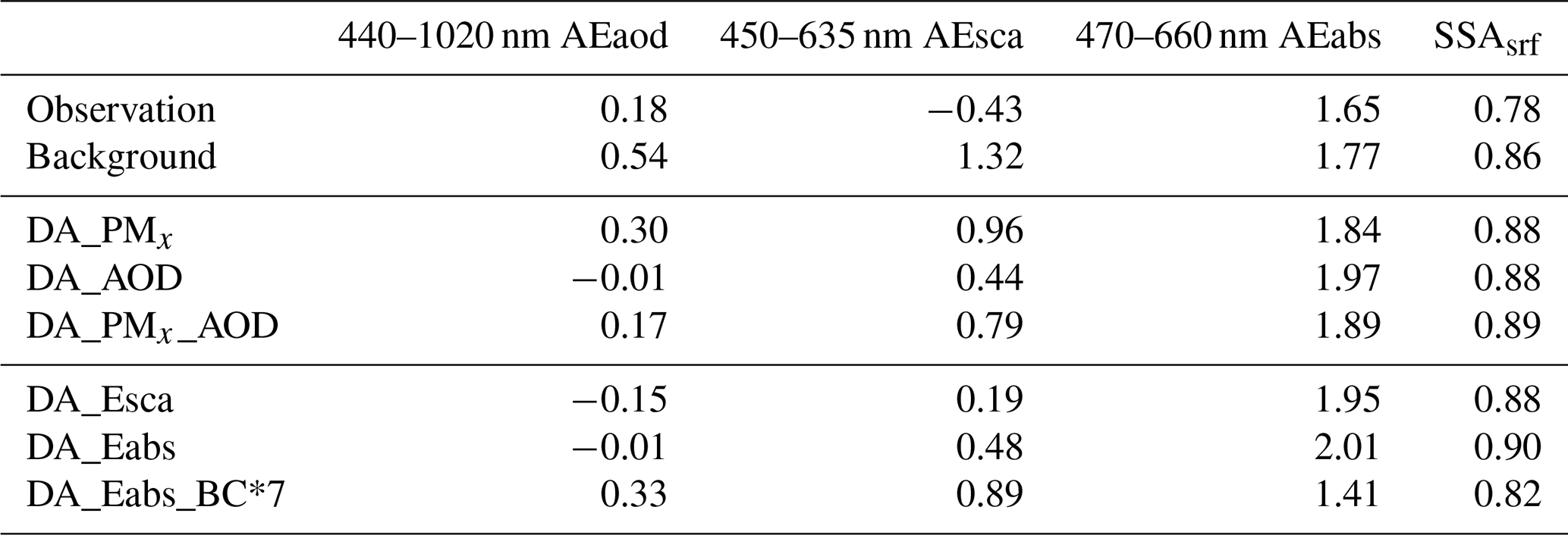
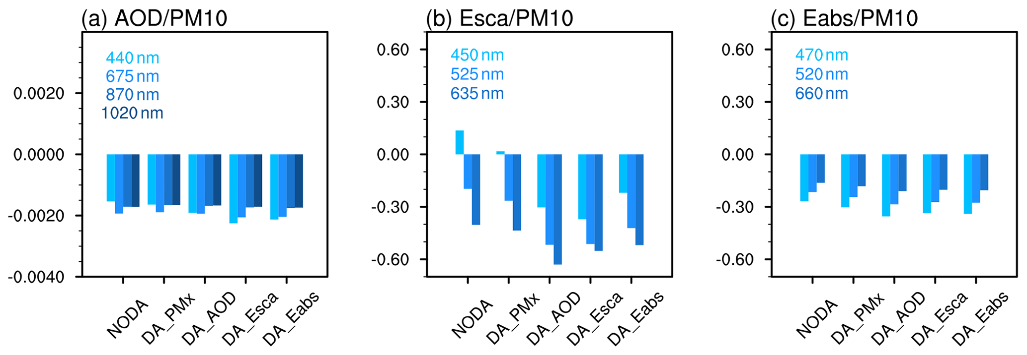
Figure 10 Mean biases in the ratio of AOD to PM₁₀, the mass scattering efficiency (Esca $/$ PM₁₀, Mm⁻¹ µg⁻¹ m³), and the mass absorbing efficiency (Eabs $/$ PM₁₀, Mm⁻¹ µg⁻¹ m³) at Kashi in April 2019.

We computed the surface single-scattering albedo (SSA_srf) with the 525 nm scattering coefficient and 520 nm absorption coefficient. We did not use the Ångström exponent to interpolate the scattering or absorption coefficients to a similar wavelength because the AE itself had a large model bias even after DA (Table 3). The observed SSA_srf value was 0.78, indicating an emphatic absorption particle, probably due to the mixture of anthropogenic black carbon and natural desert dust in the local air. The model background SSA_srf was 0.86. The DA analyses gave an even higher SSA_srf (0.88 to 0.9).

The low bias in mass scattering or absorption efficiency is related to the aerosol optical module based on Mie theory in WRF-Chem. First, the simulations used four size bin particle segregation. This coarse size representation aggregated many aerosols in the accumulation mode (Fig. 8f). Because small particles have a strong light attenuation capability, according to Mie theory, too many coarse particles would not effectively increase the AOD. Saide et al. (2020) linked the aerosol optics to the size bin representation (from 4 to 16 bins) for hazes in South Korea. They showed that WRF-Chem underestimated the dry aerosol extinction, and the underestimation could be relieved when using a finer size bin than four. Okada and Kai (2004) found that the dust particle radius in the Taklimakan Desert was in the range of 0.1–4 µm, indicating the dominant fine-mode particles in the desert.

Second, the dust particles are irregular in shape (Okada and Kai, 2004), while the spherical particle is a common assumption for the aerosol optics in Mie theory in current models, which is an essential source of uncertainty in the forward operator of WRF-Chem when the assumption of spherical particles for dust fails. The irregular morphology has a significant influence on the dust simulation. Okada et al. (2001) found that the aspect ratio (the ratio of the longest dimension to its orthogonal width) of the mineral dust particles (0.1–6 µm) in China's arid regions exhibited a median of 1.4. Dubovik et al. (2006) suggested the aspect ratio of ∼ 1.5 and higher in desert dust plumes. Kok et al. (2017) found that the dust' sphericity assumption underestimated dust extinction efficiency by ∼ 20 %–60 % for the dust particle larger than 1 µm. Tian et al. (2020) found that using a dust ellipsoid model could increase the concentration of coarse dust particle (5–10 µm) by ∼ 5 % in eastern China and ∼ 10 % in the Taklimakan area because of the decrease in gravitational settling, compared with the simulations with dust sphericity model. Nevertheless, the aspect ratio of the spheroid dust is uncertain. Even after applying the spheroidal approximation, Sorribas et al. (2015) found that the model underestimated 550 nm aerosol scattering and backscattering values by 49 % and 11 % because of the uncertainties in a particle's axial ratio, complex refractive index, and the particle size distribution. To date, the assumption of spherical particles has been widespread in models (including WRF-Chem) for computational efficiency. The impact of dust morphology on DA deserves further investigation.

To reduce the overestimate in PM_x concentrations, we set the gridded standard deviation in place of the latitude-binning standard deviation, as discussed in Sect. 2.3. Figure 11 shows the analyzed vertical profiles of PM_x concentrations. Higher PM₁₀ concentrations were shown in the low atmosphere than at the surface for the assimilation experiments. These vertical error profiles decreased the surface PM₁₀ particles and increased the PM_2.5 $/$ PM₁₀ ratio. The BEC tuning was not sufficient to increase the mass extinction efficiency to the observed value. The mass extinction efficiency in the analysis was almost equivalent to the background value (Table 4). Finer aerosol size representation and a more advanced aerosol optical calculation for dust could be considered as solutions.

Table 4 The ratios of AOD, aerosol scattering or absorption coefficient to PM₁₀ concentration (mean ± standard deviation) in the observations, the model background data, and the DA analyses.

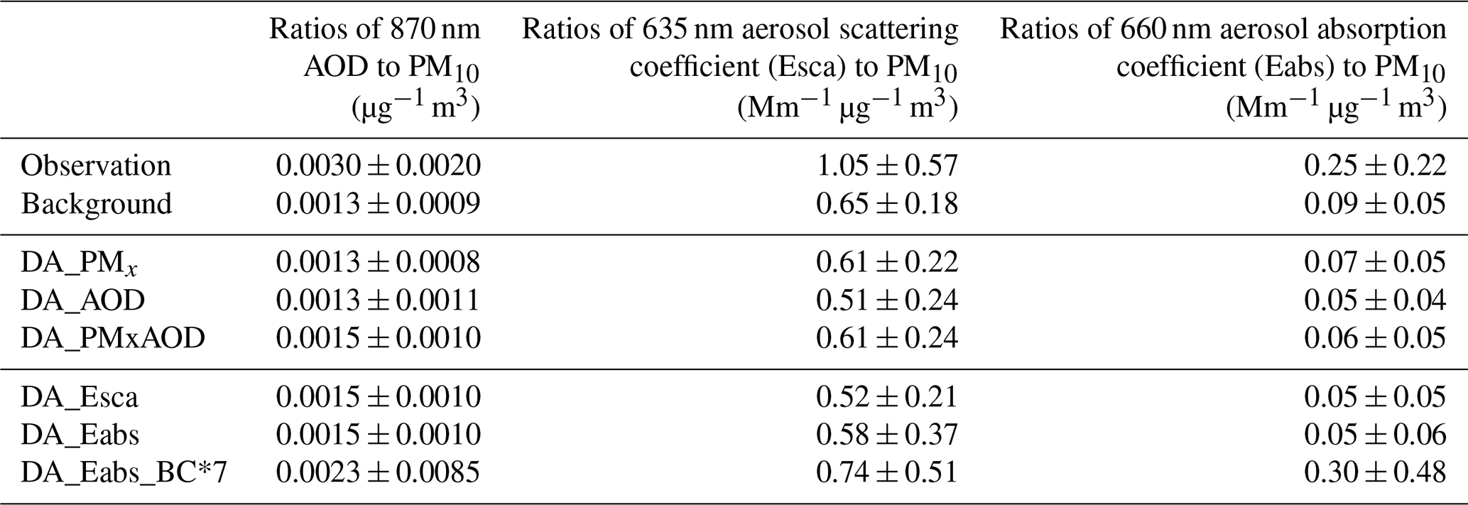
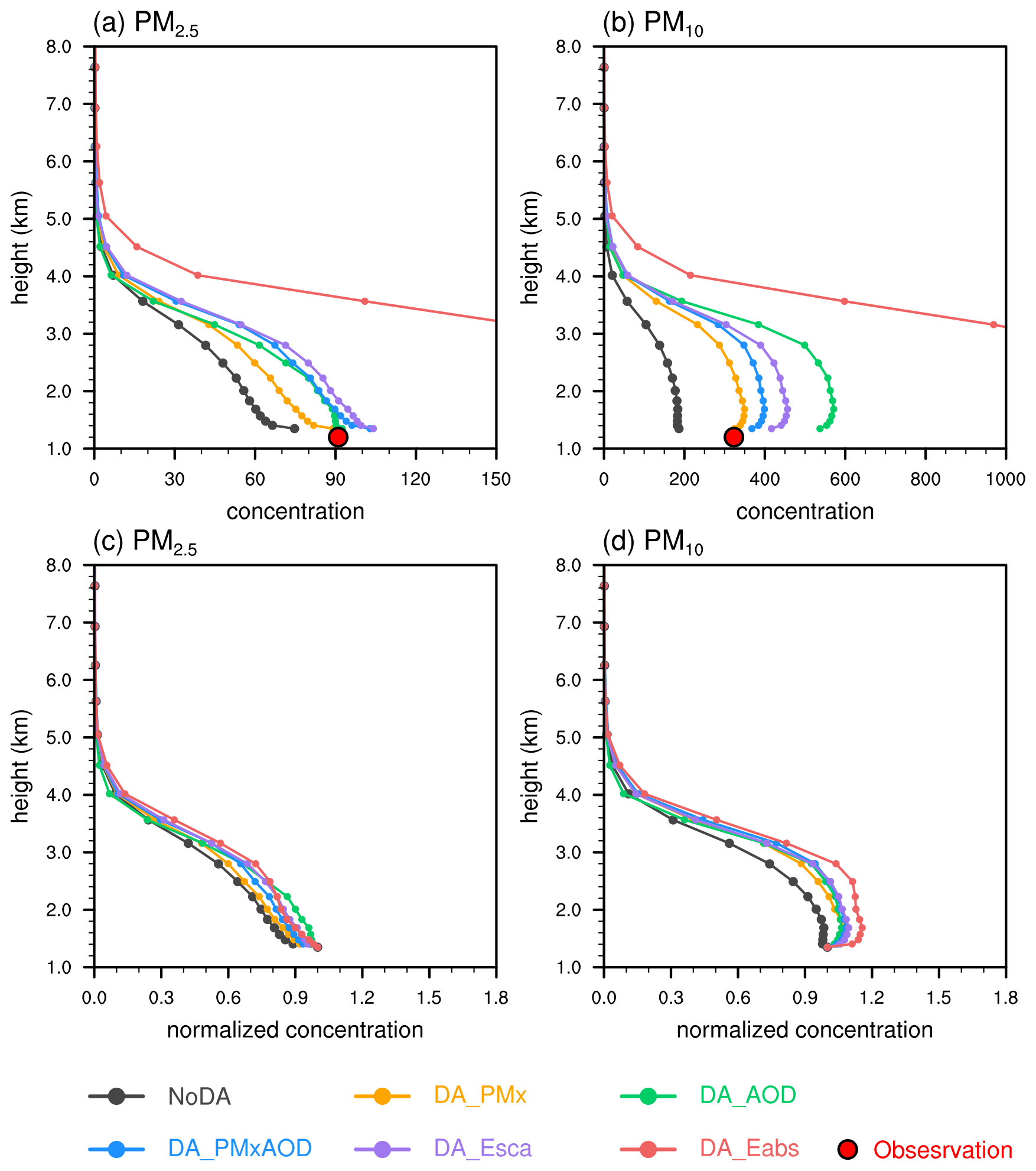
Figure 11 Mean vertical profiles of (a) PM_2.5 (µg m⁻³), (b) PM₁₀ (µg m⁻³), and their normalized concentration respect to their own surface concentrations (c, d) at Kashi in April 2019.

Assimilating the AOD seems to increase the diurnal variation in the DA analyses, but this variation was not conclusive since there were different amounts of AOD data for DA at 00:00, 06:00, and 12:00 UTC. The AOD data were not always available as the data quality control (i.e., cloud screening). There was a higher increase in the concentration at noon (06:00 UTC) (Fig. 9b), corresponding to a few high AODs during mild dust episodes at that hour. The DA system had to raise the PM₁₀ to fit the observed high AOD values. Because the CE318 AOD was only available in the daytime, no DA analysis was performed at 18:00 UTC. Also, due to the limited AOD data, assimilating AOD did not substantially increase the correlation of PM_x. The analyzed PM_2.5 and PM₁₀ still had low correlations with the observed levels (R=0.31–0.35).

3.4 Assimilating aerosol scattering coefficient

Assimilating the aerosol scattering coefficient (DA_Esca) yielded overall analyses similar to the phenomenon in DA_AOD. The analyzed 635 nm scattering coefficient (192.1 Mm⁻¹) was lower than the observation (231.5 Mm⁻¹), with a high correlation of 0.97. The low biases were smaller at short wavelengths (Fig. 10b). The wavelength-dependent biases indicated that the current DA system cannot eliminate the bias at each wavelength simultaneously. The analyzed monthly mean AOD was 0.53, better than the AOD of 0.38 when assimilating PM_x. However, the surface particle concentrations were overestimated (i.e., positive biases by 14 % for PM_2.5 and 37 % for PM₁₀), with a substantial increase in the coarse particles of OIN. Overestimations appeared during a few mild dust episodes (Fig. 7d). It indicated that WRF-Chem underestimated the dust scattering efficiency, in accordance with the low bias in the ratio of the scattering coefficient to PM₁₀ (0.52 Mm⁻¹ µg⁻¹ m³; Table 4). Thus, the DA system overfitted the PM_x concentration to approach the observed scattering coefficient. The diurnal PM₁₀ in the analysis was similar to the assimilation of PM_x, showing a maximum improvement and a robust nocturnal variation at 18:00 UTC (Fig. 9c). Assimilating the scattering coefficient failed to improve the absorption coefficient. The monthly mean absorption coefficient was 16.5 Mm⁻¹, 65 % lower than the observed value. The AE responses in DA_Esca followed those in DA_AOD. The AE values were overfitted (−0.15) for AOD, slightly improved (0.19) for the scattering coefficient, and got much larger (1.95) for absorption coefficient.

3.5 Assimilating aerosol absorption coefficient

In contrast to the above results, assimilating the absorption coefficient (DA_Eabs) deteriorated all the analyses other than the absorption coefficient. The analyses showed substantial daily variations, and strong positive biases appeared in the dust episodes (Fig. 7). The PM_2.5 was overestimated by a factor of 3, and the PM₁₀ was overestimated by a factor of 4. The increases occurred each hour (Fig. 9d). Because of the constant ratio between mass and number concentration, the particle number concentration increased. As a result, the aerosol scattering coefficient was overfitted to 612.2 Mm⁻¹, higher than the observed levels by a factor of 3. The monthly mean AOD improbably rose to 1.73. Nevertheless, the absorption coefficient (40 Mm⁻¹) was improved to the observed level (47.4 Mm⁻¹). The AE responses were similar to the results in DA_AOD, showing an overfitting (−0.01) for AOD, a slightly better value for the scattering (0.48), and a much larger value for the absorption (2.01).

Improving the absorption coefficient at the cost of PM₁₀ overestimation indicates the model biases in the representation of the particle mixture and the other absorbing particles (e.g., black carbon, brown carbon, and aged dust). The leading absorption aerosol in WRF-Chem is BC, which had the maximum absorption and hence the maximum DA modification in the second size (0.156–0.625 µm; Fig. 8e). Because the BC had a small background concentration, the BC showed a small DA improvement (< 1.5 µg m⁻³) and did not greatly enhance the particle absorption. Meanwhile, the coarse dust particle concentration was primarily increased but did not have a strong absorption as BC. As a result, the model lowered the absorption coefficient's ratio to PM₁₀ by 1 order of magnitude (0.05; Table 4). Because of the observed absorption coefficient constraint, the DA system dramatically overestimated the particle concentrations and induced too much higher aerosol scattering coefficient and AOD. The overestimated PM₁₀ lowered the mass scattering and absorption efficiencies. The mass absorption efficiency was much lower at a short wavelength (Fig. 10c), opposing the lower bias at a long wavelength for the mass scattering efficiency (Fig. 10b). The low biases were dependent on the wavelength, indicating an elaborate tuning that simultaneously eliminates the wavelength-dependent bias. It requires the DA system, for example, to add aerosol number concentration as an additional control variable and specify complex refractive index at each wavelength more precisely. The WRF-Chem aerosol simulation uses a high number of size bin representation is also helpful.

As the strong positive biases in PM_x were concerned, the scattering coefficient's overestimation was higher than that of the absorption coefficient in DA_Eabs (Table 2). As a result, DA_Eabs gave the highest SSA_srf (0.9; Table 3) in all DA experiments, the opposite of our expectation that the assimilation of absorption coefficient should decrease the positive bias in SSA.

To understand the DA_Eabs's failure, we performed a few sensitivity experiments by changing the imaginary part of the dust refractive index on 12:00 UTC on 9 April. The dust's imaginary part that we set in the experiments covers the retrieved value range of imaginary index for typical desert dust as shown in Di Biagio et al. (2019). The results are presented in the Supplement Table S4a and b. The sensitivity experiments show that a high imaginary part of the dust refractive index decreases the aerosol absorption coefficient (Table S4b). This paradox is due to the BC's reduction. Specifically, a high imaginary part increases coarse dust's absorption efficiency and decreases the coarse dust number concentration (num_a04; Table S4a). This reduction led to less fine aerosol number concentrations (e.g., num_a02) because of the inter-size bin correlation. BC is abundant in the second and third size bins, and its imaginary part of the refractive index is 2 orders of magnitude higher than dust. Less BC caused a weak absorption coefficient. By contrast, the low dust imaginary part would not greatly increase dust numbers in the coarse size bin because the DA system also attempts to increase BC in the fine particles to enhance the absorption coefficient. In an extreme case with a zero value for the imaginary part of dust, the improvement of absorption coefficient exclusively relies on BC; the num_a02 is increased by 1 order of magnitude (Table S4a), and 660 nm Eabs rose to 92.5 Mm⁻¹ (Table S4b), much higher than the observed level.

At Kashi, BC has a low background concentration and low background error. The innovation of BC was limited. Thus, tuning the imaginary part of dust's complex refractive index would not significantly change the SSA_srf value (0.89 to 0.92). Excluding the contribution from OIN in PM₁₀, the scattering coefficient was associated with sulfate. The sulfate's background error was higher than the BC's by 1 order of magnitude. The DA system prioritized sulfate modification even when assimilating the absorption coefficient, resulting in a smaller BC mass fraction in PM₁₀ (Fig. 12f) and a high SSA_srf of 0.90.

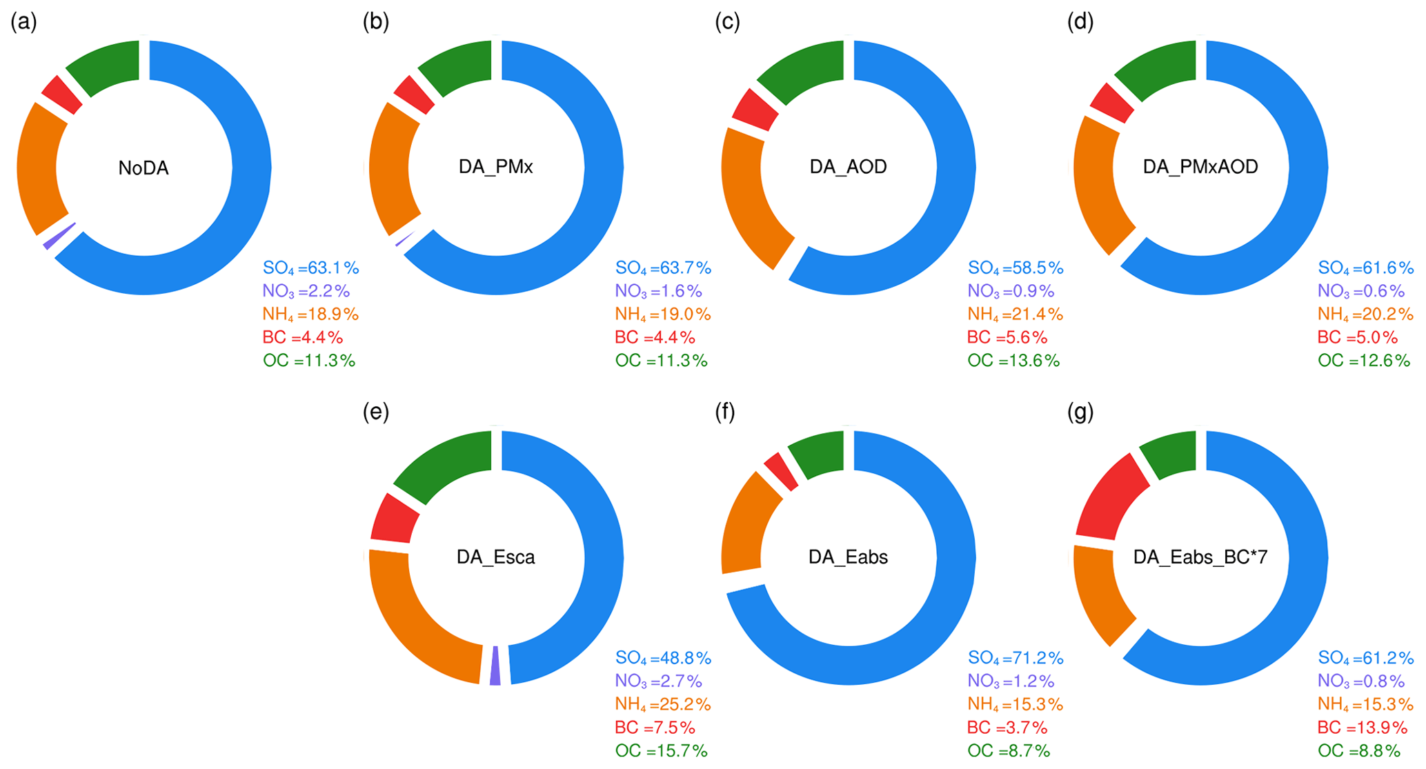
Figure 12 Mean mass percentage (%) of chemical composition in PM₁₀ excluding the OIN component at Kashi in April 2019.

We did another set of sensitivity experiments by increasing the original BC's BEC per size bin. As shown in the Supplement Table S5, increasing the BC's BECs would not much deteriorate the absorption coefficient and significantly decrease the positive biases in PM_x, AOD, and scattering coefficient; the SSA_srf approached the observation. Increasing BC's BECs by a factor of 7 (DA_Eabs_BC*7) shows the best analyses. This experiment suppressed the positive biases without decreasing the absorption coefficient's accuracy (Fig. 7), and the BC mass fraction increased (Fig. 12g). The absorption AE decreased to 1.41 (Table 3). Although the decrease was small, this change was the opposite of the increase in the absorption AE in the other DA experiments. Nevertheless, the disadvantage of the enlargement of BC's BEC is noticeable. The simultaneous assimilation of scattering and absorption coefficient is not as convergent as before. After four outer loops each with 50 inner iterations, the analyzed absorption coefficient in DA_Eabs_BC*7 was still higher than the observed value by 47 % (Fig. S1j). These results indicate a low bias in BC's background concentration that violates the prerequisite unbiased condition for the control variable in Eq. (1), and this background bias is too large to be consumed in BEC.

3.6 Assimilating multi-source observations

Assimilating an individual observation improves the corresponding model parameter (i.e., PM_2.5, PM₁₀, Esca, Eabs, and AOD) but may worsen other parameters. The reasons for the inconsistent improvements are relevant to the aerosol model itself. These are that (1) the model parameters have opposite signs in biases (e.g., one model parameter has a positive bias while another has a negative bias) and (2) the model biases have vast differences in magnitude (e.g., a good fit of a parameter may lead to another's overfit) and the different biases in magnitude cannot be reconciled because the forward operator is inaccurate in representing the linkage between aerosol mass and aerosol optics (e.g., lower particle mass extinction efficiency).

In our case, simultaneous assimilation of the scattering and absorption coefficients (DA_Esca_Eabs) resulted in the analyses when assimilating the scattering coefficient alone (DA_Esca), and the inferior analysis in DA_Eabs vanished. This was because incorporating the scattering coefficient constrained the aerosol number concentrations. DA_PMxAOD substantially improved the AE for AOD, with an analyzed value of 0.17, consistent with the observed value of 0.18 (Table 3). The scattering AE was somewhat improved (0.79), although it was still far from the observed value of −0.43. The absorption AE (1.89) was worse than the background (1.77), far deviating from the observed value of 1.65. Among the DA experiments, simultaneous assimilation of PM_x and AOD (DA_PMxAOD) gave the best DA results, in which all the analyses except the absorption coefficient were not significantly different in the monthly mean values from the observations. Simultaneous assimilation of all observations (DA_PM_x_Esca_Eabs_AOD) did not substantially improve the analyses compared with DA_PMxAOD because the surface coefficients and AOD had overlapping information on the light attenuation. A redundant information source did not introduce extra constraints on the DA system.

3.7 Vertical profiles of aerosol concentrations

Figure 11 shows the vertical concentration profiles of PM_2.5 and PM₁₀. The DA system increased the aerosol concentrations up to a height of 4 km, consistent with previous studies on the Taklimakan Desert. Meng et al. (2019) simulated a deep dust layer thickness in spring, with a 3–5 km depth. Ge et al. (2014) analyzed the Cloud-Aerosol Lidar Orthogonal Polarization data in 2006–2012 in the desert. They showed that dust could be lifted to 5 km above the Tarim Basin and even higher along the northern slope of the Tibetan Plateau. Among our DA experiments, the vertical PM₁₀ concentration increased quickly in the lowest three model layers and maintained high values at heights of less than 3 km. This vertical profile corresponded to the background vertical error profile, reflecting the deep dust transporting layer. The PM_2.5 vertical profiles showed a rapid reduction with an increase in altitude. The figure clearly shows that DA_PM_x improved the PM_2.5 and PM₁₀ better, whereas DA_AOD preferentially adjusted the coarse particles and overestimated the PM₁₀. Also shown in the figure are the vertical profiles normalized to their own respective surface particulate concentrations. The assimilations added a larger fraction of the mass in these layers and adjusted the shapes of the PM₁₀ profiles within 3 km above the ground (Fig. 11d).

4 Discussions

4.1 DA impact on aerosol chemical composition

Due to the control variable design, our DA system modifies each aerosol's chemical composition according to the BEC values. The PM₁₀ chemical fractions remain close to their background values (Fig. 12). As discussed in Sect. 3.5, the assimilation of the aerosol absorption coefficient alone (DA_Eabs) increased the sulfate fraction. Sulfate was the predominant anthropogenic aerosol at Kashi and had a high background error value. The DA system prioritized sulfate modification and prevented a rise in the BC fraction in DA_Eabs. For the enlarged BC's BEC in DA_Eabs_BC*7, the BC mass fraction showed the largest increase. The magnitude of the background error determines the analyzed aerosol chemical fraction. The total aerosol quantities' assimilation cannot eliminate the intrinsic bias in aerosol composition. Accurate aerosol chemistry and optical modules are crucial to attaining better background aerosol chemical data for DA analysis (Saide et al., 2020).

4.2 DA impact on aerosol direct radiative forcing

Table 5 shows the instantaneous clear-sky ADRF in the background data and the analyses of DA_PM_x and DA_PMxAOD. The DA effect gradually faded away after restarting the model run. Because AOD and the surface particle concentrations had different DA frequencies, we focused on the instantaneous radiative forcing values 1 h after assimilating AOD data in the two DA experiments to ensure that the comparison was based on similar analysis times. The immediate data after DA also show the effective DA effects.

Table 5 The mean instantaneous clear-sky shortwave (SW), longwave (LW), and the net (SW+LW) direct radiative forcing (W m⁻²) at the top of the atmosphere (TOA), in the atmosphere (ATM) and at the surface (SRF) in the background and the simulations restarted from the analyses of DA_PM_x and DA_PM_x_AOD at 1 h after the analysis times of AOD at Kashi in April 2019.

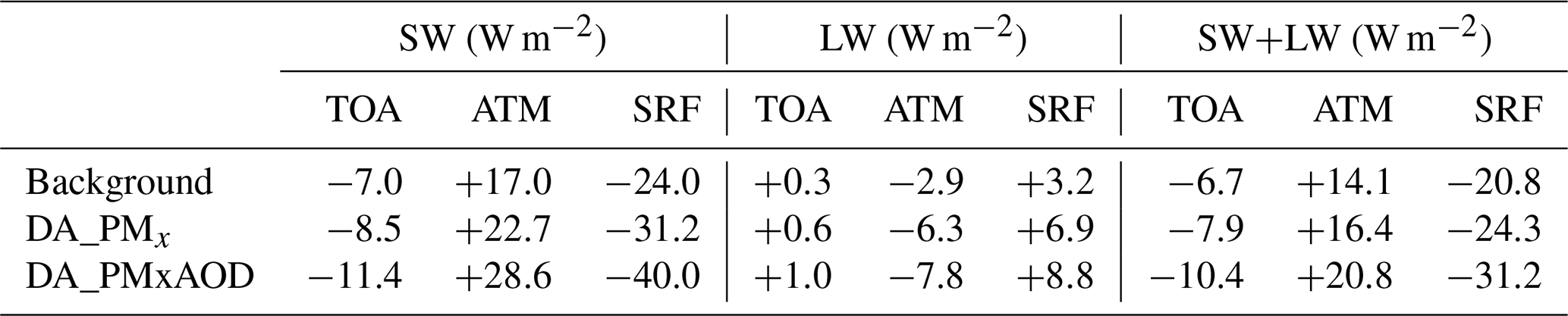
Aerosol redistributes the energy between the land and the atmosphere. The atmosphere gains more shortwave energy as the dust and black carbon particle absorption; the warming atmosphere emits more longwave energy as it absorbs shortwave energy. The change in energy budget at the surface is correspondingly the opposite of that in the atmosphere. As shown in Table 5, the enhancements in surface cooling forcings were slightly stronger than those of atmospheric warming. The difference between the surface forcing and atmospheric forcing is the ADRF at the top of the atmosphere (TOA). When assimilating the surface particle concentrations, the TOA ADRF were enhanced by 21 % in the shortwave, 100 % in the longwave, and 18 % in the net forcing values, and when assimilating the AOD, enhanced by 34 %, 67 %, and 32 %, respectively. At Kashi, the total net (shortwave plus longwave) clear-sky ADRF with assimilating surface particles and the AOD were −10.4 W m⁻² at the TOA, +20.8 W m⁻² within the atmosphere, and −31.2 W m⁻² at the surface, and they were enhanced by 55 %, 48 %, and 50 % respectively, compared to the background ADRF values.

It is noteworthy that the ADRF estimation remains uncertain even after DA. The AOD observation is only sporadically available because of cloud screening in retrieval data. The DA experiments cannot eliminate the low bias in AOD in WRF-Chem. The ADRF values in the DA experiments are likely to be weaker than the plausible aerosol radiative forcing at Kashi. Neither DA experiment lowers SSA_srf to approach the observation. Penner et al. (2001) claimed that under average conditions, an SSA less than ∼ 0.85 tends to lead to net warming. The observed SSA_srf (0.78) indicates likely aerosol warming forcing at Kashi, while WRF-Chem and the DA analyses tend to impose aerosol cooling forcing. The ADRF uncertainty is associated with the background aerosols. WRF-Chem simulates aerosol size up to 10 µm, whereas larger particles (> 10 µm) exhibit substantial absorption relative to scattering in the visible wavelength (Kok et al., 2017). Anthropogenic emission inventories need an update for the year 2019, reducing the potential low bias in BC concentration. Additionally, the revised GSI does not consider the change in particle effective radius per size bin when calculating the aerosol number concentration in each outer loop. The low absorption cross section raises aerosol number concentration as compensation, increasing the aerosol scattering coefficient too much. If our tangent operator considered the change in particle effective radius per size bin, we could use aerosol mass and number concentration as control variables simultaneously. The DA system would have higher flexibility to balance the particle radius and number concentration and improve the absorption coefficient. All these need further research in the future.

5 Conclusions

This study described our revised GSI DA system for assimilating observed aerosol data for the four size bin sectional MOSAIC aerosol mechanism in WRF-Chem. The DA system has new design tangent linear operators for the multi-wavelength AOD, aerosol scattering, and absorption coefficients measured by the sun–sky radiometer, nephelometer, and aethalometer, respectively. We examined the DA system for Kashi city in northwestern China by assimilating the multi-wavelength aerosol optical measurements gathered by the Dust Aerosol Observation–Kashi field campaign of April 2019 and the concurrent hourly measurements of surface PM_2.5 and PM₁₀ concentrations.

Our DA system includes two main aspects. Firstly, the control variable is the aerosol chemical composition per size bin corresponding to the WRF-Chem output data. This design allows modifying the composition of each aerosol based on their background error covariances. The number of control variables could be reduced by intentionally excluding a few aerosol compositions in a specific case if these compositions have low concentrations (e.g., chlorine and sodium in this study). Second, the DA system incorporates the observed AOD by assimilating the column mean aerosol extinction coefficient. This transfer avoids handling sensitivity from light attenuation length to the aerosol mass concentration in the tangent linear operator, which is difficult to accurately estimate and which introduces significant errors in the operator. The tangent linear operator for AOD has two variants that can incorporate nephelometer and aethalometer measurements at the surface.

The most abundant aerosol at Kashi in April 2019 was dust. The WRF-Chem model captured the main dust episodes but underestimated the monthly mean concentrations of PM_2.5 and PM₁₀ by 17 % and 41 %, respectively. The model failed to capture the peak concentrations from a dust storm on 24 April. The aerosol scattering or absorption coefficients and AOD in the background data showed strong low biases and weak correlations with the observed levels. The DA systems effectively assimilate the surface particle concentrations, aerosol scattering coefficients, and AOD. Some deficiencies in the DA analysis were related to the forward model bias in transferring the aerosol mass concentrations to the aerosol optical parameter. Simultaneous assimilation of the PM_2.5 and PM₁₀ concentrations improved the model aerosol concentrations, with significant increases in the coarse particles; meanwhile, the analyzed AOD was 42 % lower than observed levels. The assimilation of AOD significantly improved the AOD but overestimated the surface PM₁₀ concentration by 68 %. Assimilating the aerosol scattering coefficient improved the scattering coefficient in the analysis but overestimated the surface PM₁₀ concentration by 37 %. Therefore, it seems that WRF-Chem underestimated the aerosol extinction efficiency. As compensation, the DA system overestimated the aerosol concentration to fit the observed optical values, yielding overly high particle concentrations.

A notable problem was the assimilation of the absorption coefficient, which greatly overestimated the monthly mean values by a factor of 4 in PM₁₀. The aerosol absorption coefficient was improved but was still 16 % lower than observed values. The failure of DA analysis when assimilating the absorption coefficient is associated with many factors, including the biases of the model in aerosol particle mixture and aged dust, the uncertainties in the imaginary part of dust complex refractive index, the uncertain background error of BC, and the likely low bias in anthropogenic emissions. The most effective DA is the simultaneous assimilation of surface particle concentration and AOD, which provides the best overall DA analysis.

Our control variables' design allowed the DA system to adjust the aerosol chemical compositions individually. However, the analyzed anthropogenic aerosol chemical fractions were almost equivalent to the background chemical fractions. The reason is that the hydrophilic aerosols have equivalent or comparable refractive indices and hygroscopic parameters in the forward operator; they, therefore, have comparable tangent linear operator values when assimilating the aerosol optical data. It may be possible to separate the chemical compositions based on their background errors. The model anthropogenic aerosols were low at Kashi, probably due to the anthropogenic emissions' low biases. The low background concentrations led to low background errors and few increments for all chemical compositions. As a result, the chemical fractions of the anthropogenic aerosols remained close to their background values.

When assimilating surface particles and AOD, the instantaneous clear-sky ADRFs (shortwave plus longwave) at Kashi were −10.4 W m⁻² at the TOA, +20.8 W m⁻² within the atmosphere, and −31.2 W m⁻² at the surface. Since the DA analyses still underestimated the AOD value and overestimated SSA, the aerosol radiative forcing values assimilating the observations were underestimated in the atmosphere and the surface.

The limitations that necessitate further research include the following points:

1. The desired binning strategy should link the circulation flow and particle emission sources. A better hybrid DA coupled with the ensemble Kalman filter will be more effective for estimating the aerosol background error.

2. The observational error could be elaborated further. The PM₁₀ included the anthropogenic coarse particles, which should be separated from the dust originating from the desert (Jin et al., 2019). We set the observation errors for PM_x and AOD to the conventional values. The observational errors of the nephelometer and aethalometer were slightly arbitrary in this study, necessitating further consideration.

3. The anthropogenic aerosols' background errors are needed to harmonize better to assimilate the aerosol absorption coefficient or absorption AOD.

4. The DA system was based on four size bin MOSAIC aerosols, but it can be extended to work with eight size bin MOSAIC aerosols in WRF-Chem. When assimilating aerosol optical data, the DA quality is strongly dependent on the forward model. The responses of our DA analysis to the bias and uncertainty in the forward aerosol optical model in WRF-Chem need further investigation.