Interhemispheric transport of metallic ions within ionospheric sporadic E layers by the lower thermospheric meridional circulation

Long-lived metallic ions in the Earth's atmosphere (ionosphere) have been investigated for many decades. Although the seasonal variation in ionospheric “sporadic E” layers was first observed in the 1960s, the mechanism driving the variation remains a long-standing mystery. Here, we report a study of ionospheric irregularities using scintillation data from COSMIC satellites and identify a large-scale horizontal transport of long-lived metallic ions, combining the simulations of the Whole Atmosphere Community Climate Model with the chemistry of metals and ground-based observations from two meridional chains of stations from 1975–2016. We find that the lower thermospheric meridional circulation influences the meridional transport and seasonal variations of metallic ions within sporadic E layers. The winter-to-summer meridional velocity of ions is estimated to vary between −1.08 and 7.45 m/s at altitudes of 107–118 km between 10–60^∘ N. Our results not only provide strong support for the lower thermospheric meridional circulation predicted by a whole atmosphere chemistry–climate model, but also emphasize the influences of this winter-to-summer circulation on the large-scale interhemispheric transport of composition in the thermosphere–ionosphere.

1 Introduction

Sporadic E (E_s) layers of metallic ion plasma occur in the E region at altitudes between 90 and 130 km. Unlike other ionospheric layers, formed by the photoionization of N₂ and O₂, in which the major molecular ions NO⁺ and O${}_{\mathrm{2}}^{+}$ have lifetimes on the order of seconds, the E_s layer is composed of long-lived (up to 10 d) metallic ions (Plane et al., 2015) and is remarkably thin, typically 1–3 km thick (Layzer, 1972). Over one-third of the interruptions to the Global Positioning System (GPS) and Global Navigation Satellite System (GNSS) caused by ionospheric weather can be attributed to the E_s layer (Yue et al., 2016). One long-standing mystery is the marked seasonal variability of E_s, with a maximum between 10–60^∘ latitude in the summer hemisphere and a minimum between 60–70^∘ latitude in the winter hemisphere (Whitehead, 1989; Tsai et al., 2018; Yu et al., 2019b). The most likely explanation for the seasonal dependence of E_s layers is the wind shear, by which the seasonal variations of zonal and meridional winds in the E region above 95 km cause the summer E region to be dominated by the vertical convergence of ions but dominated by the diffusion of ions in winter (Yuan et al., 2014). Model-simulated mean divergences of the concentration flux of metallic ions by vertical wind shear are mainly distributed in the mid-latitudes of 20–40^∘ in winter (Wu et al., 2005; Chu et al., 2014; Yu et al., 2019b, 2020). A fundamental disagreement of the distribution of the E_s winter minimum exists between observations and recent model simulation, particularly when the effects of magnetic declination angle were considered (Yu et al., 2019b). Although E_s layers have been investigated since the early years of ionospheric investigations (Whitehead, 1960), their seasonal dependence cannot be explained by the vertical wind shear theory (Whitehead, 1989). This remains one of the weakest points in understanding E_s layer formation. Recently, sporadic E-like phenomena were discovered in the Martian ionosphere (Collinson et al., 2020), which indicates that understanding E_s layers and the dynamical and electrodynamical processes that perturb planetary ionospheres is very important for long-distance radio communication on Earth, Mars, and other planets.

Numerical studies indicate that there is a winter-to-summer meridional circulation in the lower thermosphere driven by gravity-wave forcing. This meridional circulation is referred to as the lower thermospheric residual mean meridional circulation (Liu, 2007). Recent modelling studies (Smith et al., 2011; Qian et al., 2017; Qian and Yue, 2017) have found clear signatures that the residual meridional circulation is important for trace gas distributions and composition variations in the thermosphere and ionosphere. However, the lower thermospheric meridional wind is considerably smaller than the amplitudes of tides (Wu et al., 2008), and thus it is difficult to directly measure and characterize.

The present paper reports a study of the global-scale winter-to-summer transport of metallic ions in the upper atmosphere from scintillation data observed by the Constellation Observing System for Meteorology, Ionosphere, and Climate (COSMIC) satellites (Anthes et al., 2008). The wind shear theory is the most likely candidate for explaining the interhemispheric transport of metallic ions within E_s layers. We extend the vertical wind shear theory (Mathews, 1998) to three dimensions, deriving the zonal, meridional, and vertical ion velocities. The large-scale horizontal transport of ions is analysed with respect to the mechanism of E_s formation and a possible impact of the winter-to-summer lower thermospheric circulation on the morphology of E_s layers. The velocity of the meridional transport of metallic ions is quantitatively estimated from two meridional chains of ground-based ionospheric monitoring stations, located roughly along the Greenwich meridian (0^∘ E) and 120^∘ E. These ionospheric observations cover a period of 35 years. The quantitative assessment is consistent with the meridional ion velocity predicted by model calculations.

2 Results

It is widely accepted that vertical wind shears in zonal and meridional neutral winds drive the vertical motion of metallic ions in the E region of the ionosphere. To better understand the meridional motion of metallic ions, the contributions to meridional and vertical ion drift from zonal (U), meridional (V), and vertical (W) winds calculated from three-dimensional wind shear theory (Eqs. A3–A5) are shown in Fig. 1. It shows that V is the main contributor to the meridional velocity of ions. The meridional wind plays a more important role than the zonal and vertical winds in meridional ion drifts.

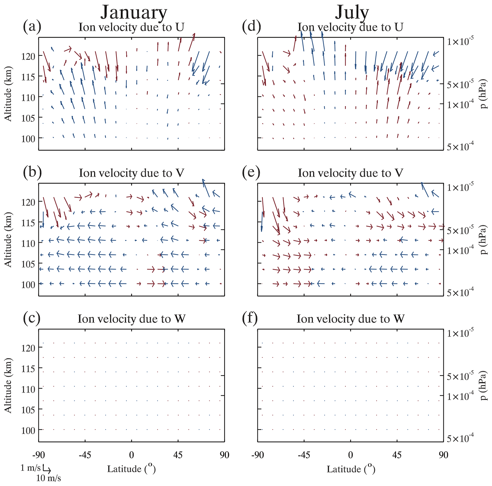
Figure 1 Ion velocity due to zonal (U), meridional (V), and vertical (W) wind in January (a–c) and July (d–f). The red arrows denote the northward ion drifts, and the blue arrows denote the southward ion drifts (vertical and meridional vectors with scale 1 m⋅s⁻¹ $/$ 10 m⋅s⁻¹).

The amplitude scintillation S4 index is one of the most important parameters in the GPS and GNSS radio occultation data, defined as the standard deviation of the normalized intensity in signals. Large S4 values indicate ionospheric plasma irregularities with strong fluctuations (Yue et al., 2015; Tsai et al., 2018), which are related to the plasma frequencies of E_s layers (Arras and Wickert, 2018; Resende Chagas et al., 2018). The E_s layer is a thin layer of enhanced plasma irregularities and is composed of metallic ions which converge vertically mainly due to wind shear (Kopp, 1997; Mathews, 1998; Grebowsky and Aiken, 2002). The E_s layer scatters, refracts, or reflects incident HF and VHF radio waves (Whitehead, 1989). It has been demonstrated that there is a universal connection between S4max occurring at heights of 90–130 km and critical frequencies of E_s layers (Yu et al., 2020, 2021a). The S4max occurring at E_s altitudes of 90–130 km is used as a proxy for the electron concentration within E_s layers (Wu et al., 2005; Yue et al., 2015; Arras and Wickert, 2018; Resende Chagas et al., 2018; Yu et al., 2019b, 2021a).

The maps in Fig. 2a and b show the geographical distribution of E_s layers represented by the S4max index for winter (December, January, February) and summer (June, July, August) based on the 6-year COSMIC multi-satellite dataset between 2006 and 2011. The most dramatic feature of the global E_s map is the pronounced summer maximum in a broad band of 10–60^∘. E_s layers are weaker in winter. The winter minimum of E_s (S4max <0.3) is observed along the 60–80^∘ geomagnetic latitude band, dividing the mid-latitude region and polar region. This typical E_s seasonal dependence has been revealed in both hemispheres over the past few decades from ground-based ionosonde, radar, and satellite measurements (Whitehead, 1989; Mathews, 1998; Wu et al., 2005; Haldoupis et al., 2007; Arras et al., 2008; Chu et al., 2014; Yu et al., 2019b, 2020).

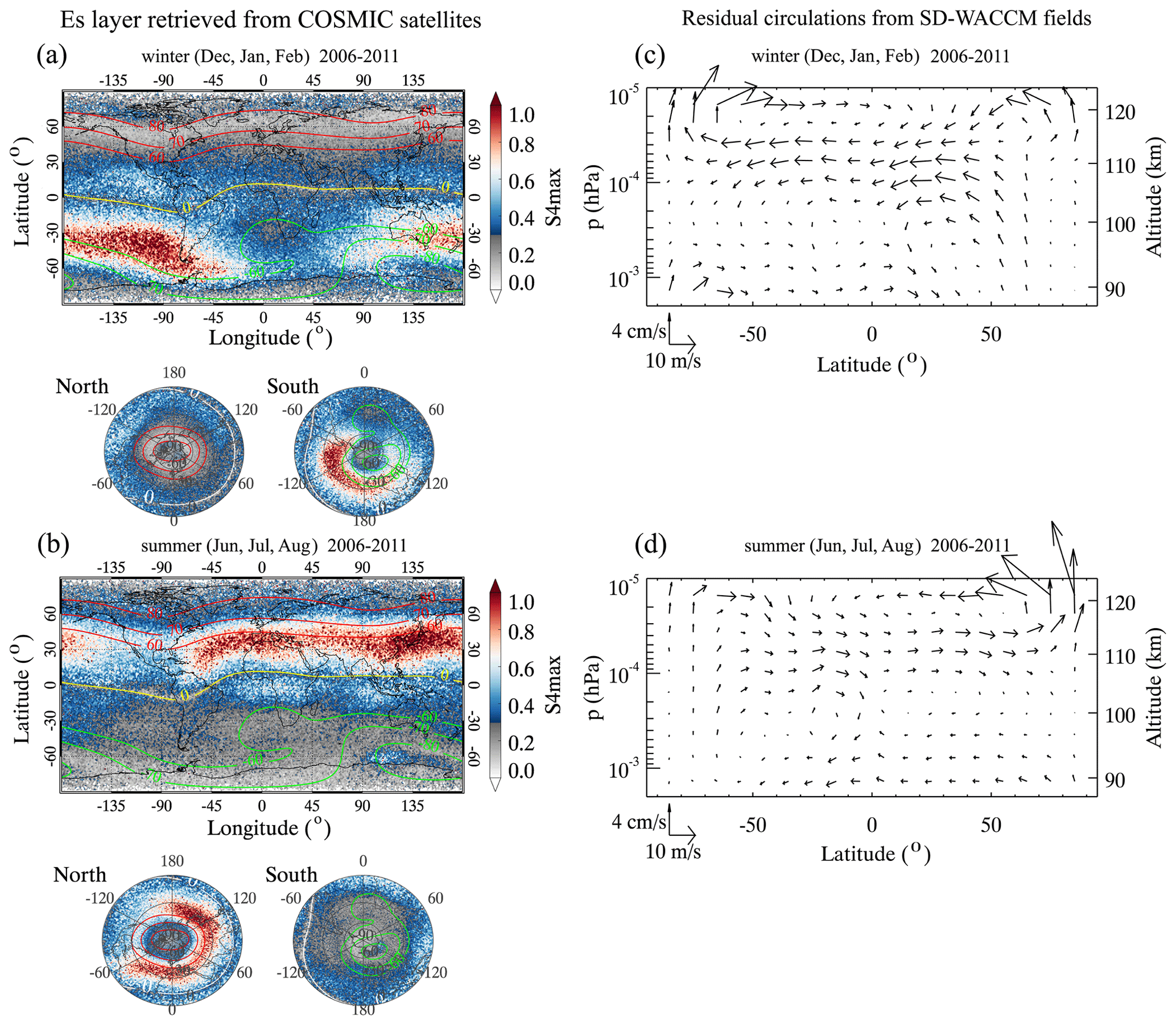
Figure 2 Global distributions of the mean E_s layer intensity represented by the S4max index from COSMIC are shown in (a) and (b) for the winter (December, January, February) and summer (June, July, August), respectively, between 2006 and 2011, detected from COSMIC multi-satellites with a resolution of a 1${}^{\circ }\times \mathrm{1}{}^{\circ }$. The red and green curves represent the geomagnetic latitude contours of 60, 70, and 80^∘ in the Northern Hemisphere and Southern Hemisphere, and the yellow curve represents the geomagnetic Equator. The mean residual circulations are calculated for winter (c) and summer (d) using the SD-WACCM4 (2006–2011). There are three circulation cells: mesospheric circulation, lower thermospheric circulation, and thermospheric circulation. Below 95 km, the summer-to-winter mesospheric circulation is driven by gravity-wave forcing. Between 95 and 115 km, the winter-to-summer lower thermospheric circulation is driven by gravity-wave forcing that is in the opposite direction to that which drives the mesospheric circulation. Above 115 km, the solar-driven thermospheric circulation is a summer-to-winter circulation.

Figure 2c and d show the atmospheric circulation in winter and summer averaged from 2006–2011, which has been calculated using SD-WACCM4. Three circulation cells are apparent, which are consistent with previous studies (Qian et al., 2017; Qian and Yue, 2017). Below ∼95 km, the summer-to-winter mesospheric circulation is driven by gravity-wave forcing. Between ∼95 and ∼115 km, the winter-to-summer lower thermospheric circulation is driven by gravity-wave forcing that is in the opposite direction to that which drives the mesospheric circulation. Above ∼115 km, the thermospheric circulation is a summer-to-winter circulation driven by solar extreme ultraviolet (EUV) heating.

Figure 3 shows the monthly mean variations in the intensity of E_s layers represented by the S4max index from COSMIC, with superposed ion drifts from the model. The observations of E_s layers from satellites suggest that the maximum E_s latitude has an interhemispheric migration to the summer hemisphere. These E_s seasonal variations have been known for over 50 years (Smith, 1968), but the cause is unknown (Whitehead, 1989; Yu et al., 2019b). The plot also shows a north-south asymmetry (the northern summer peak is stronger than the southern summer peak). The solid green lines are the ratios of column densities of E_s intensities at different latitudes to the global mean column density. Vertical wind shear alone does not account for the variations in relative column densities in E_s layers. The column density of E_s layers should not vary much from month to month if the E_s seasonal dependence is just a result of seasonal variations in vertical wind shears that favour ion convergences in different areas. The peak of the relative column densities shows an interhemispheric transport. This seasonal dependence is consistent with interhemispheric transport of long-lived metallic ions by the winter-to-summer lower thermospheric meridional circulation. The yellow arrows between 100 and 120 km show the predicted meridional and vertical velocity of ion drift from three-dimensional wind shear theory (Eq. A4 and A5) driven by the atmospheric meridional circulations. Above 100 km, metallic ions have a lifetime of at least several days in the thermosphere (Plane et al., 2015). At altitudes of 90–100 km, the lifetime of ions rapidly decrease to timescales of hours to minutes because the ions are able to form molecular ions (principally metal oxide ions through reaction with O₃). Therefore, the predicted velocity of metallic ions is calculated only above 100 km.

Figure 3 Monthly variation in the E_s layer intensity represented by the S4max index from COSMIC, with superposed ion drifts from the model caused by residual meridional circulations. The monthly mean variations in E_s layers are shown for different altitudes and latitudes from 2006 to 2011. The solid green lines are the ratios of column densities at different latitudes to the global mean column density. The yellow arrows between altitudes of 100–120 km show the predicted vertical and meridional velocity of ion drift (vectors with a scale of 1 m⋅s⁻¹ $/$ 10 m⋅s⁻¹), driven by the atmospheric meridional circulations from the SD-WACCM4.

It is found that the observed E_s seasonal variation correlates strongly with the ion meridional transport caused by the winter-to-summer lower thermospheric circulation. From February to April, the E_s moves from both hemispheres toward the Equator with a large equatorward ion drift speed over 10 m/s. Following this, E_s moves northward from May to July and reaches a strong summer maximum in accordance with the wind shear in the lower thermospheric circulation that predicts the winter-to-summer interhemispheric transport of ions. From August to January, E_s migrates toward the Equator with the equatorward metallic ion velocity, followed by a subsequent summer peak in the Southern Hemisphere with a southward ion velocity. Further evidence for a link between the seasonal variation and ion meridional transport is a distinctive northern high-latitude depression of E_s, which is not well explained by the vertical wind shear effects in previous experimental and theoretical studies (Arras et al., 2008; Chu et al., 2014; Yu et al., 2019b). The dissipative region of E_s during winter solstice agrees with the location at which the mean meridional wind splits between 60 and 70^∘ N (Fig. 2c). According to multi-satellite observations and simulation results, the seasonal variation in E_s could be highly dependent on the meridional transport of metallic ions, which is inseparable from the ion dynamics of E_s formation with wind shear effects.

In addition to neutral winds, the electric field also plays an important role in the transport of metallic ions (Nygren et al., 1984; Bristow and Watkins, 1991; Bedey and Watkins, 2001; Huba et al., 2019; Kirkwood and Nilsson, 2000). A global atmospheric model of meteoric iron (WACCM-Fe) (Feng et al., 2013) reproduces the global seasonal variations of Fe⁺ density over the altitude range of E_s layers. The E×B drift and Coulomb force-induced ion drift (Cai et al., 2019) associated with the electric field are derived from standard WACCM X (Liu et al., 2018), and the seasonal variation of global distribution of Fe⁺ is from WACCM Fe (Feng et al., 2013). Figure 4 shows the monthly mean Fe⁺ flux ${\mathrm{\Phi }}_{{\text{Fe}}^{+}}$, calculated offline from WACCM X and WACCM Fe. The corresponding latitude–height plots and maps of Fe⁺ flux due to E×B drift, Coulomb force-induced ion drift, and neutral winds in January and July are shown in Fig. 4a–b and c–d. The colour scale denotes the meridional Fe⁺ flux and extends from −1 (southward) to +1 (northward). This clearly shows a convergence of Fe⁺ flux between 105 and 115 km at 25–45^∘ S in winter and 25–45^∘ N in summer. The horizontal red lines in Fig. 4a and c represent the altitude of 106 km at which the peak density of E_s layers reaches its maximum value and the lower thermospheric meridional circulation dominates. Figure 4b and d show the Fe⁺ flux at this height as a function of latitude and longitude. The Fe⁺ meridional flux is mostly southward in winter (typically $-\mathrm{3.3}\times {\mathrm{10}}^{\mathrm{7}}$ to $-\mathrm{2.3}\times {\mathrm{10}}^{\mathrm{9}}$ m⁻²s⁻¹) and northward in summer (typically 1.6×10⁷ to 4.9×10⁹ m⁻²s⁻¹).

Figure 4 (a) Zonal mean latitude–height plot of Fe⁺ flux ${\mathrm{\Phi }}_{{\text{Fe}}^{+}}$ (m⁻² s⁻¹) calculated offline from WACCM X and WACCM Fe in January, adding E×B drift, Coulomb force-induced ion drift, and neutral wind effects. The colour scale denotes the meridional Fe⁺ flux and extends from −1 (southward) to +1 (northward). Also plotted are ion flux vectors that combine the meridional Fe⁺ flux with the vertical Fe⁺ flux. The horizontal red line represents the altitude of 106 km at which the peak density of E_s layer reaches its maximum value. (b) Map of Fe⁺ flux at an altitude of 106 km from the model in January. Panels (c) and (d) show a zonal mean latitude–height plot and map of Fe⁺ flux, respectively, from the model in July.

Although a variety of ground-based measurements have been performed, most studies interpret observations of earth metallic species in vertical and small-scale transport processes (Macleod, 1966; Plane, 2003; Davis and Johnson, 2005; Johnson and Davis, 2006; Davis and Lo, 2008; Haldoupis, 2012; Chu et al., 2014; Yu et al., 2015; Cai et al., 2017; Yu et al., 2017, 2019a). It is especially important to further monitor the ion-drift motions generated by meridional flows. Signatures in E_s seasonal variations by ion interhemispheric transport were investigated using the two meridional chains of low-latitude to mid-latitude ionosonde stations as shown in Fig. 5a. Figure 5b–c show the long-term time series of E_s layers at each station. The daily mean intensities of E_s layers, found by taking a monthly moving average, are plotted using red to blue colours, corresponding to the low-latitude to mid-latitude stations. Specifically, all 10 stations exhibit a strong summer peak, which appears earlier at the low-latitude stations than at the mid-latitude stations. This trend can be used to quantitatively estimate the ion velocity of winter-to-summer interhemispheric transport.

Figure 5 (a) Ground-based measurements of E_s from two meridional chains of low-latitude to mid-latitude ionosondes. There are 10 ionosonde stations in these two meridional chains, roughly along the Greenwich meridian (b) and 120^∘ E (c). These ionospheric observations started in 1975. A 35-year dataset is analysed to try to identify the signature of the large-scale horizontal transport of metallic ions in E_s, induced by meridional circulations.

In Fig. 6, green and red points represent annual summer peaks for 10 stations from two meridional chains. Each point represents a day of year (DOY) of the E_s summer maximum. The mean DOY for summer peaks is shown as a box, with the error bar representing the standard error in this mean. An estimation of ion meridional transport was made from the variations in peak time with latitude. Linear fits are presented using measurements from the Greenwich meridional chain (green line), 120^∘ E longitudinal chain (red line), and a total of 10 stations (blue line). A linear correlation is found in the Greenwich meridional chain (correlation coefficient: r=0.38). The p value is 0.53 calculated for testing the hypothesis of no correlation. The slope is 8.06±0.15^∘/d (10.35±0.19 m/s), indicating winter-to-summer ion transport. This value is slightly larger than the predicted meridional velocity in Fig. 3; −1.08–7.45 m/s between 10–60^∘ N in summer. The slope from the 120^∘ E longitudinal chain is 0.99±0.29^∘/d $\sim \mathrm{1.27}\pm \mathrm{0.37}$ m/s (r=0.99, p<0.01), which is within the predicted range of ion meridional velocity. This velocity is lower than that from the Greenwich meridional chain, and this is thought to be due to the differences in the magnitude of meridional flows between different solar cycles. The blue line represents the fit for all 10 stations (r=0.67, p=0.04). The estimated ion meridional velocity is 3.16±0.13^∘/d (4.06±0.17 m/s). In modelling studies, the dynamics of the lower thermospheric meridional circulation are much less understood than the well-known mesospheric meridional circulation (Liu, 2007; Qian et al., 2017; Qian and Yue, 2017). It is difficult to directly measure the mean meridional wind since the lower thermospheric meridional circulation is considerably smaller than the tidal amplitudes (Wu et al., 2008). The results presented here show that the atmospheric circulation has a marked influence on the meridional transport and seasonal variations of the metallic ions in E_s layers. There is also some evidence that the magnitude of the meridional flows may vary with longitude.

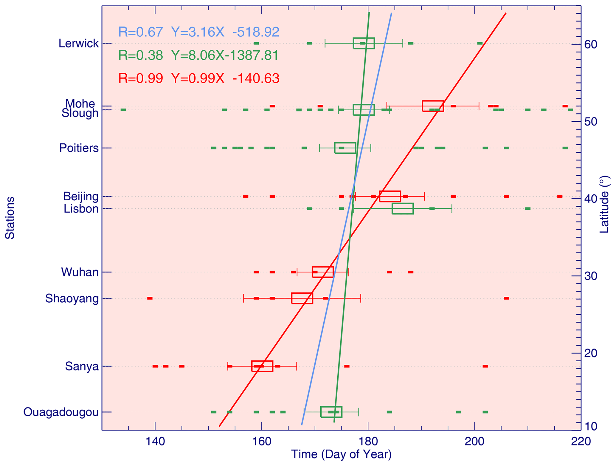
Figure 6 Latitudes of stations versus the mean day-of-year (DOY) time of the annual summer peaks for 10 stations from two meridional chains during 1975–2016. The ionosonde stations cover 10–60^∘ N. Green and red points are the annual summer peaks, and each point represents a DOY of a E_s summer peak. The mean DOY time of summer peaks is shown as a box, with the error bar representing the standard error in this mean for each station. The green, red, and blue lines show the linear fits between the peak time and latitude, using measurements from the Greenwich meridional chain, 120^∘ E longitudinal chain, and the total of all 10 stations, respectively. The linear fit relationship and correlation coefficient are also given, from which an ion meridional velocity in a meridional chain could be quantitatively estimated.

3 Conclusions

The lower thermospheric winter-to-summer meridional circulation is a process that has generally been ignored, although it plays a fundamental role, comparable to the vertical wind shear, in the transport of metallic ions throughout the Earth's upper atmosphere and ionosphere. Two differences should be noted though, i.e. the distribution of metallic ions and the formation of the E_s. The former is determined by the transport, as demonstrated here in this study, while the latter is probably directly tied to shear. The large-scale horizontal transport of metallic ions needs to be considered over seasonal-to-interannual timescales in global-scale studies of metallic species, and this provides a mechanism that explains the observed E_s seasonal variations (Whitehead, 1960). In addition to the interhemispheric transport, a comprehensive explanation for E_s production requires the use of a whole atmosphere climate model, including all the necessary chemistry and electrodynamics of metallic species. Global models of meteoric metals in the upper atmosphere have been developed by adding the metal chemistry into WACCM (Marsh et al., 2013; Feng et al., 2013; Wu et al., 2019). The results presented here provide an important dynamical constraint for modelling studies that aim to simulate the variations in composition of the thermosphere and ionosphere on seasonal and interannual timescales.

Appendix A: Methods

A1 Satellite and ground-based observations

The COSMIC multi-satellite dataset was used to investigate the global morphology of E_s layers during the period 2006–2011. For this we used the COSMIC-GPS amplitude scintillation index S4 (Yu et al., 2020), including the maximum S4 index (S4max), as well as the latitude, longitude, altitude, and time at which S4max was detected.

The long-term ground-based observations of intensities of E_s layers represented by the critical frequencies f_oE_s from two meridional chains of low-latitude to mid-latitude ionosonde stations were used in this study. These are five ionospheric sounders (ionosondes) located roughly along the Greenwich meridian (0^∘ E) at Lerwick (60.13^∘ N, 1.18^∘ W), Slough (51.51^∘ N, 0.60^∘ W), Poitiers (46.57^∘ N, 0.35^∘ E), Lisbon (38.72^∘ N, 9.27^∘ W), and Ouagadougou (12.37^∘ N, 1.53^∘ W) between 1975 and 1998 and five digital ionosondes (digisondes) (Bibl and Reinisch, 1978) located roughly along 120^∘ E longitude at Mohe (52.0^∘ N, 122.5^∘ E), Beijing (40.3^∘ N, 116.2^∘ E), Wuhan (30.5^∘ N, 114.4^∘ E), Shaoyang (27.1^∘ N, 111.3^∘ E), and Sanya (18.3^∘ N, 109.4^∘ E) between 2006 and 2016 under the Chinese Meridian Project (Wang, 2010).

A2 Atmospheric meridional circulations and three-dimensional wind shear theory

The atmospheric meridional circulations are calculated using the Whole Atmosphere Community Climate Model (WACCM). These circulations are the summer-to-winter mesospheric circulation, the winter-to-summer lower thermospheric circulation, and the summer-to-winter circulation. WACCM is a global climate model with interactive chemistry, developed at the National Center for Atmospheric Research. A specified dynamics version of WACCM4 (SD-WACCM4) (Marsh et al., 2013) is used. SD-WACCM4 is constrained by relaxing the temperature and horizontal winds to those from the Modern-Era Retrospective Analysis for Research and Applications, which is a NASA reanalysis for the satellite era by a major new version of the Goddard Earth Observing System Data Assimilation System Version 5 (Rienecker et al., 2011).

It is widely accepted that the mechanism for E_s formation at mid-latitudes is wind shear. From the vertical wind shear theory (Mathews, 1998), the vertical motion of metallic ions by the neutral winds is described by Eq. (A1):

$$\begin{array}{}\text{(A1)}& w_{\mathrm{i}}={\displaystyle \frac{r_{\mathrm{i}}\cos I}{\mathrm{1}+r_{\mathrm{i}}^{\mathrm{2}}}}\times U-{\displaystyle \frac{\sin I\cos I}{\mathrm{1}+r_{\mathrm{i}}^{\mathrm{2}}}}\times V+{\displaystyle \frac{r_{\mathrm{i}}^{\mathrm{2}}+{\sin }^{\mathrm{2}}I}{\mathrm{1}+r_{\mathrm{i}}^{\mathrm{2}}}}\times W,\end{array}$$

where w_i represents the vertical velocity of ions; I represents the dip angle of the geomagnetic field B (positive in the downward direction in the Northern Hemisphere); r_i is the ratio of the ion-neutral collision frequency (ν_i) to the ion gyrofrequency (ω_i); and V_n ($U,V,W$) represents the neutral wind in zonal (positive for eastward), meridional (positive for northward), and vertical (positive for upward).

From Eq. (A1), which describes the classical wind shear theory, the zonal and meridional winds act upon the vertical plasma convergence of metallic ions at all altitudes, as weighted by the ratio r_i of ν_i to ω_i. However, the meridional component of ion velocity should also be included in the wind shear theory. The formation of an E_s layer is controlled fully by the ion dynamics and expressed through a basic ion momentum equation (Chimonas and Axford, 1968) (Eq. A2 below). The steady-state ion momentum equation includes the ion-neutral collision and geomagnetic Lorentz forces:

$$\begin{array}{}\text{(A2)}& m_{\mathrm{i}}{\displaystyle \frac{\mathrm{d}{\mathit{v}}_{\mathrm{i}}}{\mathrm{d}t}}=\mathrm{0}=e(\mathit{E}+{\mathit{v}}_{\mathrm{i}}\times \mathit{B})-m_{\mathrm{i}}{\mathit{\nu }}_{\mathrm{i}}({\mathit{v}}_{\mathrm{i}}-{\mathit{V}}_{\mathrm{n}}),\end{array}$$

where m_i is the ion mass, B(Bsin Dcos I, Bcos Dcos I, −Bsin I) is the magnetic field, I and D are the dip angle and declination angle of the magnetic field, v_i (u_i, v_i, w_i) is the ion drift velocity, and V_n ($U,V,W$) is the neutral wind. We derive the ion drift in the zonal, meridional, and vertical directions from Eq. (A2) by adopting an east, north, and vertically upward Cartesian coordinate system, respectively. When the electric filed E is neglected, a conventional presentation of the wind shear theory is derived. As the vertical wind shear is described in the vertical component, we refer to this extended view of the formation and transport of the layering process as “generalized wind shear theory” with three-dimensional motions of ion drift:

$$\begin{array}{}\text{(A3)}& {\displaystyle }\begin{array}{rl}{u}_{\mathrm{i}}& ={\displaystyle \frac{r_{\mathrm{i}}^{\mathrm{2}}+{\sin }^{\mathrm{2}}D{\cos }^{\mathrm{2}}I}{\mathrm{1}+r_{\mathrm{i}}^{\mathrm{2}}}}U+{\displaystyle \frac{-r_{\mathrm{i}}\sin I+\sin D\cos D{\cos }^{\mathrm{2}}I}{\mathrm{1}+r_{\mathrm{i}}^{\mathrm{2}}}}V\\ & -{\displaystyle \frac{r_{\mathrm{i}}\cos D\cos I+\sin D\sin I\cos I}{\mathrm{1}+r_{\mathrm{i}}^{\mathrm{2}}}}W,\end{array}\text{(A4)}& {\displaystyle }\begin{array}{rl}{v}_{\mathrm{i}}& ={\displaystyle \frac{r_{\mathrm{i}}\sin I+\sin D\cos D{\cos }^{\mathrm{2}}I}{\mathrm{1}+r_{\mathrm{i}}^{\mathrm{2}}}}U+{\displaystyle \frac{r_{\mathrm{i}}^{\mathrm{2}}+{\cos }^{\mathrm{2}}D{\cos }^{\mathrm{2}}I}{\mathrm{1}+r_{\mathrm{i}}^{\mathrm{2}}}}V\\ & +{\displaystyle \frac{r_{\mathrm{i}}\sin D\cos I-\cos D\sin I\cos I}{\mathrm{1}+r_{\mathrm{i}}^{\mathrm{2}}}}W,\end{array}\text{(A5)}& {\displaystyle }\begin{array}{rl}{w}_{\mathrm{i}}& ={\displaystyle \frac{r_{\mathrm{i}}\cos D\cos I-\sin D\sin I\cos I}{\mathrm{1}+r_{\mathrm{i}}^{\mathrm{2}}}}U\\ & -{\displaystyle \frac{r_{\mathrm{i}}\sin D\cos I+\cos D\sin I\cos I}{\mathrm{1}+r_{\mathrm{i}}^{\mathrm{2}}}}V+{\displaystyle \frac{r_{\mathrm{i}}^{\mathrm{2}}+{\sin }^{\mathrm{2}}I}{\mathrm{1}+r_{\mathrm{i}}^{\mathrm{2}}}}W.\end{array}\end{array}$$

The contributions to meridional and vertical ion drift from U, V, and W in January and July are shown separately in Fig. 1. Both U and V are the main contributors to vertical ion velocity. The ion dynamics become collision dominated (r_i≫1) below 125 km altitude (Mathews, 1998). Therefore, the U term on the right of Eq. (A5) is more important than the V term, representing the relative dominant role of U in comparison with V in the vertical motion of ions. The second term with V of Eq. (A4) is more important than the other terms, representing the dominant V contribution to the meridional velocity of ions.