the Creative Commons Attribution 4.0 License.
the Creative Commons Attribution 4.0 License.
 | 10 Mar 2021
Attribution of the accelerating increase in atmospheric methane during 2010–2018 by inverse analysis of GOSAT observations
Yuzhong Zhang
Daniel J. Jacob
Joannes D. Maasakkers
Tia R. Scarpelli
Jian-Xiong Sheng
Lu Shen
Melissa P. Sulprizio
Jinfeng Chang
A. Anthony Bloom
Shuang Ma
John Worden
Robert J. Parker
Hartmut Boesch
We conduct a global inverse analysis of 2010–2018 GOSAT observations to better understand the factors controlling atmospheric methane and its accelerating increase over the 2010–2018 period. The inversion optimizes anthropogenic methane emissions and their 2010–2018 trends on a grid, monthly regional wetland emissions, and annual hemispheric concentrations of tropospheric OH (the main sink of methane). We use an analytical solution to the Bayesian optimization problem that provides closed-form estimates of error covariances and information content for the solution. We verify our inversion results with independent methane observations from the TCCON and NOAA networks. Our inversion successfully reproduces the interannual variability of the methane growth rate inferred from NOAA background sites. We find that prior estimates of fuel-related emissions reported by individual countries to the United Nations are too high for China (coal) and Russia (oil and gas) and too low for Venezuela (oil and gas) and the US (oil and gas). We show large 2010–2018 increases in anthropogenic methane emissions over South Asia, tropical Africa, and Brazil, coincident with rapidly growing livestock populations in these regions. We do not find a significant trend in anthropogenic emissions over regions with high rates of production or use of fossil methane, including the US, Russia, and Europe. Our results indicate that the peak methane growth rates in 2014–2015 are driven by low OH concentrations (2014) and high fire emissions (2015), while strong emissions from tropical (Amazon and tropical Africa) and boreal (Eurasia) wetlands combined with increasing anthropogenic emissions drive high growth rates in 2016–2018. Our best estimate is that OH did not contribute significantly to the 2010–2018 methane trend other than the 2014 spike, though error correlation with global anthropogenic emissions limits confidence in this result.
- Article
(5015 KB) - Full-text XML
-
Supplement
(1427 KB) - BibTeX
- EndNote


Methane is the second most important anthropogenic greenhouse gas after CO2, with an emission-based radiative forcing of 0.97 W m−2 since preindustrial times (Myhre et al., 2013). Methane is emitted to the atmosphere from a range of anthropogenic activities including fuel exploitation, agriculture, waste and wastewater treatment, and biomass burning. The main natural source is from wetlands, with minor contributions from geological seeps, forest fires, and termites. Atmospheric methane has a lifetime of 11.2±1.3 years against tropospheric oxidation by the hydroxyl radical (OH) (Prather et al., 2012). Minor sinks include stratospheric loss, oxidation by Cl atoms, and absorption by soils (Kirschke et al., 2013).
Unlike the steady rise in atmospheric CO2, the rise of methane has taken place in fits and starts. Observations from the NOAA network (Dlugokencky, 2020) (https://www.esrl.noaa.gov/gmd/ccgg/trends_ch4/, last access: 22 June 2020) show a period of stabilization in the early 2000s, followed by renewed growth after 2007 that has accelerated since 2014. Annual growth rates averaged 0.50 % a−1 for 2014–2018 compared to 0.32 % a−1 for 2007–2013. The growth of atmospheric methane concentrations, if continued at current rates in coming decades, may significantly negate the climate benefit of CO2 emission reduction (Nisbet et al., 2019).
However, our understanding of the drivers behind the methane growth rate is still limited, preventing reliable projections for future changes. Explanations have differed for the renewed growth of atmospheric methane since 2007. A concurrent increase in atmospheric ethane has been interpreted as evidence of an increase in oil and gas emissions (Hausmann et al., 2016; Franco et al., 2016). However, the assumption that the ethane-to-methane emission ratio should be stable is questionable (Lan et al., 2019). Meanwhile, a concurrent shift towards isotopically lighter methane has been attributed to an increase in microbial sources either from livestock or wetlands (Schaefer et al., 2016; Nisbet et al., 2016). Worden et al. (2017) pointed out that the trend towards isotopically lighter methane could be explained by decreases in fire emissions that are isotopically heavy. Based on methyl chloroform observations, Turner et al. (2017) and Rigby et al. (2017) suggested that a decrease in the OH sink may be the cause of the methane regrowth.
To better interpret the methane budget and its recent trends, we present an inverse analysis of global 2010–2018 methane observations from the GOSAT instrument. GOSAT provides a long record (starting in 2009) of global high-quality observations of column methane mixing ratios (Kuze et al., 2016; Buchwitz et al., 2015). A number of inverse analyses previously used GOSAT observations to constrain methane emission estimates (Fraser et al., 2013; Monteil et al., 2013; Cressot et al., 2014; Alexe et al., 2015; Turner et al., 2015; Pandey et al., 2016, 2017a; Miller et al., 2019; F. Wang et al., 2019a; Lunt et al., 2019; Maasakkers et al., 2019; Janardanan et al., 2020; Tunnicliffe et al., 2020; Yin et al., 2020). Maasakkers et al. (2019) used 2010–2015 GOSAT observations to optimize gridded methane emissions, global OH concentrations, and their 2010–2015 trends. They concluded that increasing methane emissions were driven mainly by India, China, and tropical wetlands. Our analysis is based on that of Maasakkers et al. (2019) but extends it to 2018 in order to interpret the post-2014 acceleration. We implement for that purpose a number of major improvements to the Maasakkers et al. (2019) methodology including in particular (1) separate optimization of subcontinental wetland emissions to resolve their seasonal and interannual variability, (2) correction of stratospheric methane forward model biases based on ACE-FTS solar occultation satellite data (Waymark et al., 2014), (3) prior estimates of global fuel exploitation emissions using national reports submitted to the United Nations Framework Convention on Climate Change (UNFCCC) (Scarpelli et al., 2020), and (4) optimization of annual hemispheric OH concentrations.
2.1 GOSAT observations
The observation vector for the inversion (y) consists of column-averaged dry-air methane mole fractions during 2010–2018 observed by the TANSO-FTS instrument on board the Greenhouse Gases Observing Satellite (GOSAT) (Kuze et al., 2009). The satellite is in polar sun-synchronous low-Earth orbit and observes methane by nadir solar backscatter in the 1.65 µm shortwave infrared absorption band. Observations are made at around 13:00 local solar time. We use the University of Leicester version 9 CO2 proxy retrieval (Parker et al., 2020a). The retrieval has been extensively validated against ground-based column observations from the Total Carbon Column Observing Network (Wunch et al., 2011). Validation has also been performed for the model XCO2 used in the CO2 proxy retrieval (Parker et al., 2015) and for a specific region (i.e., the Amazon) against aircraft profile observations (Webb et al., 2016). Overall, the retrieval has a single-observation precision of 13.7 ppb and a regional bias of 4 ppbv (Parker et al., 2020a), which is sufficient for a successful methane inversion (Buchwitz et al., 2015). The inversion ingests a total of 1.5 million successful GOSAT retrievals. Previous inversions of GOSAT data often excluded high-latitude observations because of seasonal bias, large retrieval errors at low solar elevations, and forward model errors for the stratosphere (Bergamaschi et al., 2013; Turner et al., 2015; Z. Wang et al., 2017; Maasakkers et al., 2019). The exclusion of high-latitude observations limited the capability of the inversions to resolve emissions at high latitudes such as from boreal wetlands and oil and gas activity in Russia (Maasakkers et al., 2019). Here we use an improved model bias correction scheme (Sect. 2.5) and include these high-latitude observations in the inversion.
2.2 State vector
The state vector (x) is the ensemble of variables that we seek to optimize in the inversion. In this work, the state vector includes (1) mean 2010–2018 methane emissions from non-wetland sources (all anthropogenic and natural emissions excluding wetlands) on a global grid (1009 elements), (2) linear trends of non-wetland emissions on that same grid (1009 elements), (3) wetland emissions from 14 subcontinental regions for individual months (1512 elements) (Fig. 1), and (4) annual mean tropospheric OH concentrations in the Northern and Southern Hemisphere (18 elements). The reason to treat wetland and non-wetland emissions separately is that wetland emissions have large seasonal and interannual uncertainties (compared to anthropogenic emissions); coarsening the spatial resolution when optimizing wetland emissions allows us to estimate monthly values for individual years (Bloom et al., 2017). This is a significant improvement over the inverse analysis of Maasakkers et al. (2019), wherein interannual and seasonal errors in prior wetland emissions were not addressed by the inversion.
Another improvement in the state vector definition relative to Maasakkers et al. (2019) is to optimize annual mean OH concentrations in each hemisphere rather than just globally. Y. Zhang et al. (2018) previously found with an observing system simulation experiment that it should be possible to constrain annual mean hemispheric OH concentrations from satellite methane observations. Patra et al. (2014) suggested that global chemical transport models (CTMs) are often biased in their inter-hemispheric OH gradient relative to methyl chloroform observations, and such bias, if not corrected, would propagate to the solution for methane emissions.
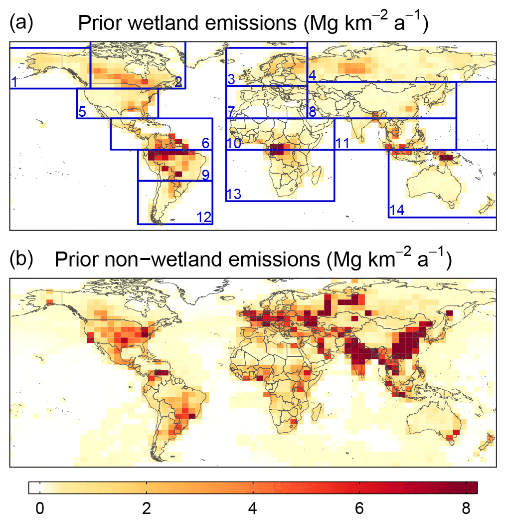
Figure 1Spatial distribution of mean 2010–2018 methane emissions used as prior estimates in the inversion of GOSAT data. The top panel shows wetland emissions, and the bottom panel shows non-wetland emissions. Blue boxes indicate the 14 subcontinental regions for which wetland emissions are optimized for individual months (Sect. 2.2): (1) Alaska + western Canada, (2) eastern Canada, (3) northern Europe, (4) Siberia, (5) temperate North America, (6) Latin America, (7) the Mediterranean, (8) East Asia, (9) the Amazon, (10) sub-Saharan Africa, (11) tropical South Asia, (12) Argentina, (13) southern Africa, and (14) Indonesia + Australia.
2.3 Prior estimates
Prior estimates for methane sources and sinks (xa) are compiled from an ensemble of bottom-up studies. Figure 1 shows the spatial distribution of prior emission estimates. For gridded anthropogenic emissions, we use as default the EDGAR v4.3.2 global emission inventory for 2012 (https://edgar.jrc.ec.europa.eu/, last access: 1 December 2017) (Janssens-Maenhout et al., 2017). We supersede it for the US with the gridded version of the Environmental Protection Agency greenhouse gas emission inventory for 2012 (Maasakkers et al., 2016). We further supersede it globally for fuel (oil, gas, and coal) exploitation with the inventory of Scarpelli et al. (2020) for 2012, which spatially disaggregates the national emissions reported to the United Nations Framework Convention on Climate Change (UNFCCC) (https://di.unfccc.int/, last access: 22 June 2020). All anthropogenic emissions are assumed to be aseasonal, except manure management for which we apply local temperature-dependent corrections (Maasakkers et al., 2016) and rice cultivation for which we apply gridded seasonal scaling factors from B. Zhang et al. (2016).
For the prior estimates of natural emissions, we take monthly wetland emissions during 2010–2018 from the WetCHARTS v1.0 extended ensemble mean (Bloom et al., 2017) for each subcontinental domain in Fig. 1. To test the impact of wetland spatial distribution within the subcontinental domains on inversion results, we performed a sensitivity inversion in which prior WetCHARTS emissions in Africa (regions 10 and 13 in Fig. 1) are increased by a factor of 3 in the Sudd wetland of South Sudan and decreased by a factor of 2.5 in the Congo Basin, following Lunt et al. (2019) and as shown in Fig. S1. Daily global emissions from open fires are taken from GFEDv4s (van der Werf et al., 2017), which accounts for high methane emissions from peatland fires (Liu et al., 2020). For geological sources, we scale the spatial distribution from Etiope et al. (2019) to a global total of 2 Tg a−1 inferred from preindustrial-era ice core 14CH4 data (Hmiel et al., 2020). Termite emissions are from Fung et al. (1991), totalling 12 Tg a−1.
The prior estimates for 2010–2018 trends in non-wetland emissions are specified as zero on the grid, except for interannual variability in fire emissions given by GFEDv4s. In this manner, all information on the posterior estimate of anthropogenic emission trends is from the GOSAT observations.
The prior estimates for the hemispheric tropospheric OH concentrations are based on a GEOS-Chem full chemistry simulation (Wecht et al., 2014). The monthly 3-D OH concentration fields from this full chemistry simulation are also used in the forward model. We optimize hemispheric OH concentrations as the methane loss frequency [s−1] due to oxidation by tropospheric OH (ki) in the Northern and Southern Hemisphere (i= north or south):
where is methane number density [molec. cm−3], v is volume, and cm3 molec.−1 s−1 is the temperature-dependent oxidation rate constant (Burkholder et al., 2015). In this definition, the denominator of Eq. (1) integrates over the entire atmosphere, and the numerator integrates over the hemispheric troposphere. Hence, global methane loss frequency (or inverse lifetime; k) due to oxidation by tropospheric OH can be expressed as the sum of hemispheric values (, where τ is the global lifetime due to oxidation by tropospheric OH). Our prior estimates from Wecht et al. (2014) are 0.050 a−1 for knorth and 0.043 a−1 for ksouth, which translates to a τ of 10.7 years and a north-to-south inter-hemispheric OH ratio of 1.16. In comparison, the methyl chloroform proxy infers τ of 11.2±1.3 years (Prather et al., 2012) and an inter-hemispheric ratio in the range 0.85–0.98 (Montzka et al., 2000; Prinn et al., 2001; Krol and Lelieveld, 2003; Bousquet et al., 2005; Patra et al., 2014), while the ACCMIP model ensemble yields a τ of 9.7±1.5 years and an inter-hemispheric ratio of 1.28±0.10 (Naik et al., 2013).
The Bayesian inversion requires error statistics for the prior estimates. The prior error covariance matrix (Sa) is constructed as follows. For mean non-wetland emissions, we assume 50 % error standard deviation for individual grid cells and 20 % for each source category when aggregated globally. For linear trends in non-wetland emissions, we specify an absolute error standard deviation of 5 % a−1 for individual grid cells. For wetland emissions, we take the full error covariance structure (including spatial and temporal error covariance) derived from the WetCHARTs ensemble members for the 14 subcontinental regions (Bloom et al., 2017). For annual hemispheric OH concentrations, we assign 5 % independent errors for individual years on top of a 10 % error for the 2010–2018 mean.
2.4 Forward model
We use the GEOS-Chem CTM v11.02 as a forward model (F) for the inversion (Wecht et al., 2014; Turner et al., 2015; Maasakkers et al., 2019) that relates atmospheric methane observations (y) to the state vector to be optimized (x) as y=F(x). The simulation is conducted at horizontal resolution with 47 vertical layers (∼30 layers in the troposphere) and is driven by 2009–2018 MERRA-2 meteorological fields (Gelaro et al., 2017) from the NASA Global Modeling and Assimilation Office (GMAO). The prior simulation is conducted from 2010 to 2018. The initial conditions are from Turner et al. (2015) with an additional 1-year spin-up starting from January 2009 to establish methane gradients driven by synoptic-scale transport (Turner et al., 2015). We further set the initial conditions on 1 January 2010 to be unbiased by removing the zonal mean biases relative to GOSAT observations. Thus, we attribute any model departures from observations over the 2010–2018 period in the inversion to errors in sources and sinks over that period.
We use archived 3-D monthly fields of OH concentrations from a GEOS-Chem full chemistry simulation (Wecht et al., 2014) to compute the removal of methane from oxidation by tropospheric OH. Other minor loss terms include stratospheric oxidation computed with archived monthly loss frequencies from the NASA Global Modeling Initiative model (Murray et al., 2012), tropospheric oxidation by Cl atoms computed with archived Cl concentration fields from X. Wang et al. (2019b), and monthly soil uptake fields from Murguia-Flores et al. (2018). The inversion does not optimize these minor sinks. The loss from oxidation by Cl is 5.5 Tg a−1, accounting for ∼1 % of methane loss. It is lower than the previous estimate of 9 Tg a−1 (Sherwen et al., 2016) used by Maasakkers et al. (2019) but is consistent with a recent analysis of methane and CO isotopic signatures (Gromov et al., 2018). Use of monthly soil uptake fields from the Murguia-Flores et al. (2018) climatology of 2000–2009 data is another update relative to Maasakkers et al. (2019) and yields a global soil sink of 34 Tg a−1.
2.5 Forward model bias correction
The GEOS-Chem-simulated methane columns have a latitude-dependent background bias relative to the GOSAT data (Turner et al., 2015). This is thought to result from excessive meridional transport in the stratosphere, a common problem in global models (Patra et al., 2011). In particular, coarse-resolution global models have difficulty resolving polar vortex dynamics that control the distribution of stratospheric methane in the winter–spring hemisphere (Stanevich et al., 2020). The GEOS-Chem model evaluation with stratospheric sub-columns derived from ground-based TCCON measurements shows that the stratospheric bias varies seasonally (Saad et al., 2016). Previous GEOS-Chem-based inversions of GOSAT data (Turner et al., 2015; Maasakkers et al., 2019) developed correction schemes by fitting differences between the prior model simulation and background GOSAT observations as a second-order polynomial function of latitude. However, these correction schemes did not consider the seasonal variation of the stratospheric biases. Moreover, they could falsely attribute high-latitude model–GOSAT differences to stratospheric model bias rather than to errors in prior emissions. Therefore, previous studies excluded high-latitude observations from their analyses (Turner et al., 2015; Maasakkers et al., 2019).
Here we improve the stratospheric bias correction by using satellite observations from ACE-FTS v3.6 (Waymark et al., 2014; Koo et al., 2017). ACE-FTS is a solar occultation instrument launched in 2003 that measures vertical profiles of stratospheric methane (Bernath et al., 2005). We compute correction factors to GEOS-Chem stratospheric methane sub-columns as a function of season and equivalent latitude based on the ratios of stratospheric methane sub-columns between the ACE-FTS and GEOS-Chem prior simulation for 2010–2015 (Fig. 2). A global scaling factor (1.06) is applied to these correction factors to enforce mass conservation for methane in the stratosphere so that the correction does not introduce a spurious stratospheric source and sink in the model simulation. We use equivalent latitude, computed on the 450 K isentropic surface from MERRA-2 reanalysis fields, as one of the predictors for parameterization. The equivalent latitude is a coordinate based on potential vorticity (PV) that maps PV to latitude based on areas enclosed by PV isopleths (Butchart and Remsberg, 1986), and it is often used to represent the influence of high-altitude dynamics (e.g., polar vortex) on chemical tracers (Engel et al., 2006; Hegglin et al., 2006; Strahan et al., 2007). We use the same stratospheric bias correction for all years because the correction does not vary significantly for individual years (Fig. S2). Figure 2 shows that GEOS-Chem model biases are largely confined to high latitudes of the winter–spring hemisphere. By having our correction factors be dependent on equivalent latitude and season, we specifically account for the overly weak polar vortex dynamical barrier in the model as the cause of the stratospheric bias (Stanevich et al., 2020).
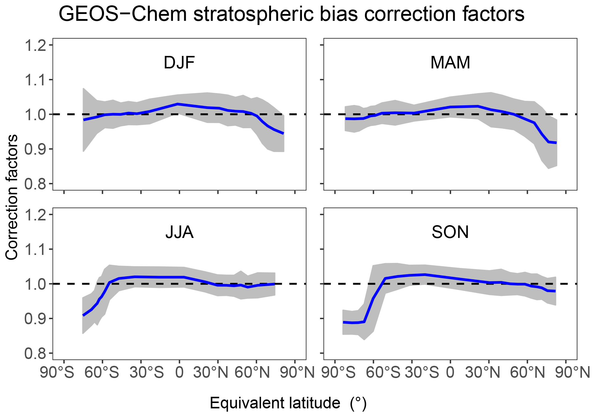
Figure 2GEOS-Chem stratospheric bias correction based on ACE-FTS observations. The figure shows the ACE-FTS to GEOS-Chem ratio of stratospheric methane sub-columns as a function of equivalent latitude and season, averaged over the 2010–2015 period. Grey shading represents the fitting uncertainty.
2.6 Inversion procedure
We perform the inversion by minimizing the Bayesian cost function (Brasseur and Jacob, 2017):
Here, the Jacobian matrix is a linearized description of the forward model (F) that relates y (observations) to x (state vector). We explicitly compute the Jacobian matrix by perturbing each individual element of x independently in GEOS-Chem simulations and calculating the sensitivity of y to that perturbation. xa is the prior estimate for x and Sa is the prior error covariance matrix (Sect. 2.3). SO is the observation error covariance matrix including contributions from the instrument error and the forward model error. We take SO to be diagonal and compute the variance terms from the statistics of the residual error (, where the overbar denotes annual averages in a grid cell) that represents the random component of model–observation differences (Heald et al., 2004). This method of constructing SO has been previously applied to GOSAT observations by Turner et al. (2015) and Maasakkers et al. (2019). The observational error standard deviation derived in this manner averages 13 ppbv. γ is the regularization parameter taken to be 0.05 following Y. Zhang (2018) and Maasakkers et al. (2019) to account for missing error covariance structure in SO.
Minimizing J(x) (Eq. 2) by solving analytically (Rodgers, 2000; Brasseur and Jacob, 2017) yields a best posterior estimate of the state vector () and the associated posterior error covariance matrix () characterizing the error statistics of :
From there we derive the averaging kernel matrix describing the sensitivity of the solution to the true state:
The trace of the averaging kernel matrix is referred to as the degrees of freedom for signal (DOFS) (Rodgers, 2000) and represents the number of independent pieces of information on the state vector that are constrained by the inversion. We refer to the diagonal terms of A as averaging kernel sensitivities, which measure the ability of the observations to quantify the individual elements of the state vector (Sheng et al., 2018c; Maasakkers et al., 2019).
The posterior solution is often presented in reduced dimensionality. For example, spatially resolved emission and trend estimates on the grid can be aggregated to countries, regions, or global and/or regional emissions from individual source sectors (oil and gas, livestock, etc.). Let W be a matrix that represents the linear transformation from the full state vector to a reduced state vector. The posterior estimation of the reduced state vector () is computed as
with posterior error covariance matrix
and averaging kernel matrix
where is the pseudo-inverse of W. The regional and global budget terms and their error covariance structures obtained by using this approach are consistent with the full inversion. In the case of aggregation by sectors, we construct W on the basis of the relative contribution of the sector to the prior emissions in each grid cell. This does not assume that the prior distribution of sectoral emissions is correct, only that the relative allocation within a given grid cell is correct.
We conduct a posterior simulation driven by the optimized (posterior) distributions of methane emissions, emission trends, and OH concentrations to evaluate the inversion. The posterior simulation results are compared with the training data (GOSAT) and independent evaluation data including TCCON total column measurements (https://tccondata.org/, last access: 22 June 2020) (Wunch et al., 2011) and NOAA surface measurements (https://www.esrl.noaa.gov/gmd/ccgg/flask.php, last access: 22 June 2020) (Dlugokencky et al., 2020). Figure 3 shows the GEOS-Chem comparison to the GOSAT data. As expected for a successful inversion, the posterior simulation achieves a better fit to GOSAT observations than the prior simulation both spatially and temporally, with root mean square errors reduced by 70 % (prior: 44 ppbv; posterior: 13 ppbv). The prior simulation shows a negative bias that grows with time and has a large seasonal structure presumably associated with errors in wetland emissions. The prior biases also have prominent spatial patterns, particularly in the extratropical Northern Hemisphere and the tropics. All these error features largely vanish in the posterior simulation through the optimized adjustment of the state vector (Fig. 3).

Figure 3Difference in methane columns between GEOS-Chem simulations and GOSAT observations. Results are shown for GEOS-Chem using prior (a, c) and posterior (b, d) state vector estimates as well as for the spatial distribution averaged during 2010–2018 (a, b) and monthly time series of zonal means in different latitude bands (c, d). Note the different color scales in (a) and (b). Tick marks on the x axes in (c) and (d) represent January in each year. Figure S6 plots panel (d) in an expanded ordinate scale.
Figure 4 presents evaluations against independent 2010–2018 observations from TCCON and NOAA sites arranged by latitude. Values are shown as the root mean square error (RMSE) for individual sites. Figure 4 shows that the inversion substantially improves the agreement between simulations and observations for all TCCON sites and almost all NOAA surface sites. Average root mean square errors are reduced by 60 % for TCCON sites (prior: 38 ppbv; posterior: 15 ppbv) and by 42 % for NOAA surface sites (prior: 43 ppbv; posterior: 25 ppbv). The seasonal component of the errors (root mean square errors computed from monthly mean model–observation differences after annual mean biases are removed; not shown in the figure) is reduced on average by 42 % for TCCON sites (prior: 6.5 ppbv; posterior: 3.8 ppbv) and 30 % for surface sites (prior: 10 ppbv; posterior: 7 ppbv), primarily owing to optimized seasonal variations in wetland emissions. In addition, we do not find large interannual variability of posterior biases that could be associated with climate oscillations such as ENSO (Fig. S3).
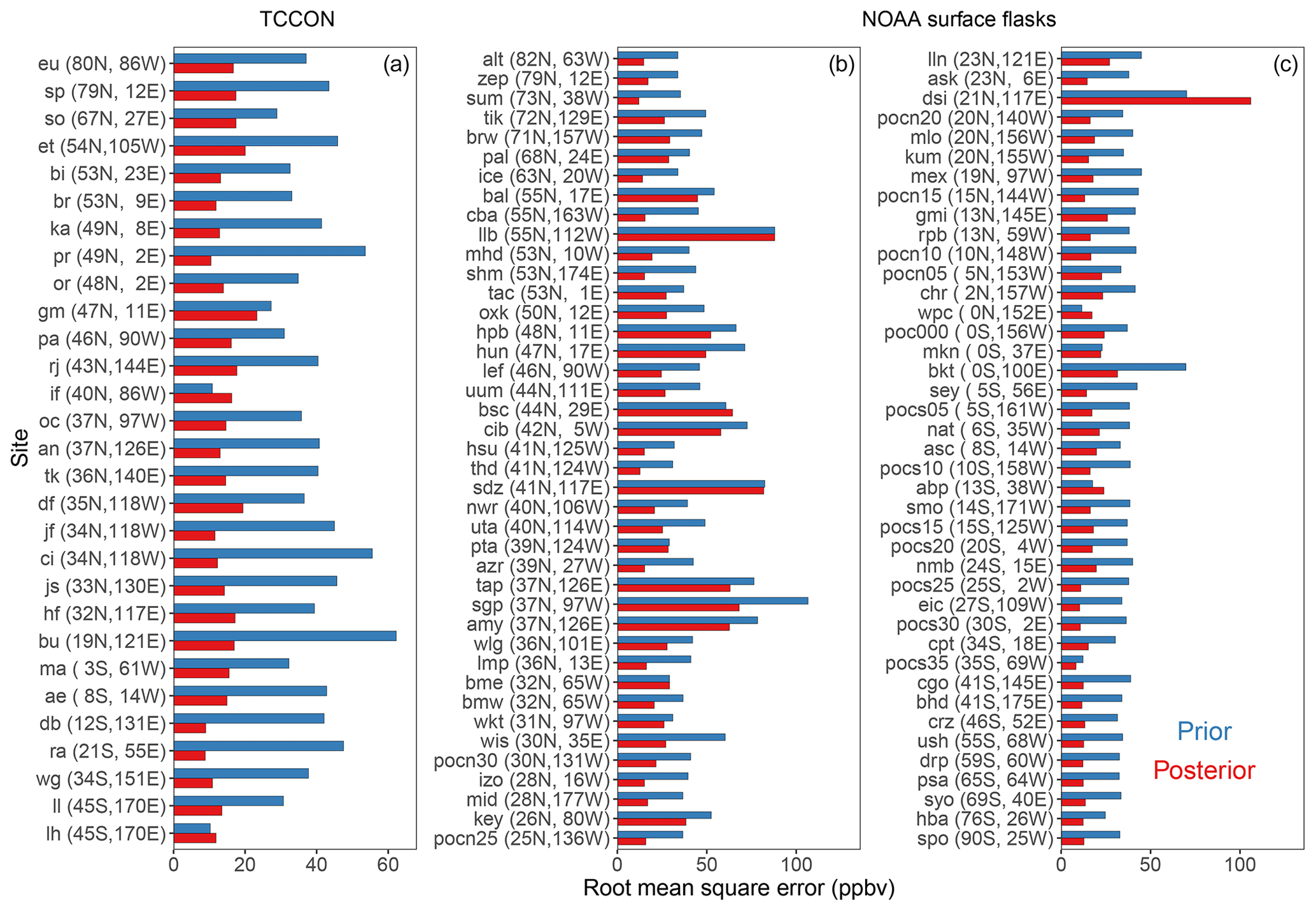
Figure 4Root mean square errors of prior and posterior GEOS-Chem simulations relative to TCCON observations of dry column methane mixing ratios (a) and NOAA observations of surface air mixing ratios (b, c). Observation sites are arranged by latitude. Data are for 2010–2018. Site names are shown along with their latitude and longitude (more information about these sites can be found at https://tccon-wiki.caltech.edu/ – last access: 22 June 2020 and https://www.esrl.noaa.gov/gmd/dv/site/index.php?program=ccgg – last access: 22 June 2020). A mountaintop TCCON site located at Zugspitze, Germany (zs; ∼3000 m a.s.l.), is excluded because the terrain effect on the total column is not resolved by the coarse-resolution model.
The posterior error covariance matrix resulting from analytically solving the Bayesian problem allows us to analyze the error structure of posterior estimates. Figure 5 plots the posterior joint probability density functions (PDFs) for pairs of global budget terms and their trends (computed following Eqs. 6–7). A strong negative error correlation in the inversion results is found between global anthropogenic emissions and methane lifetime (), reflecting the limited ability of the inversion to separate the two. In contrast, error correlations between wetland emissions and methane lifetime () as well as between wetland and anthropogenic emissions () are much smaller. We find moderate error correlations between the OH trend and either wetland or anthropogenic emission trends (). Improved separation of global budget terms and their trends may be achieved by including additional information from surface observations (Lu et al., 2020) and from thermal infrared satellite observations (Y. Zhang et al., 2018).

Figure 5Error correlations between global anthropogenic emissions, wetland emissions, and tropospheric OH concentrations (methane lifetime against oxidation by tropospheric OH; τ) in the inverse solution. Results are shown for both 2010–2018 mean values and 2010–2018 trends. The error correlations are presented as joint probability density functions for pairs of reduced global state vector elements. Confidence ellipses represent a probability of 0.1 (innermost) to 0.9 (outermost) at intervals of 0.1. The error correlation coefficients are inset.
Figure 6 further examines the error aliasing of estimates for anthropogenic and wetland emissions within or between regions. For this analysis, anthropogenic emissions optimized on the grid are aggregated to 14 subcontinental regions used for estimating wetland emissions. We find only moderate negative error correlations ( to −0.5) between estimates for anthropogenic and wetland emissions within the same region (diagonal of top left quadrant), suggesting that the inversion is able to separate the two. Cross-region error correlations are generally small for anthropogenic emissions (bottom left quadrant of Fig. 6) but have a complex structure for wetland emissions (top right quadrant of Fig. 6). For example, errors are positively correlated between sub-Saharan Africa and southern Africa wetlands (r=0.6) but are negatively correlated between eastern Canada and northern Europe wetlands ().
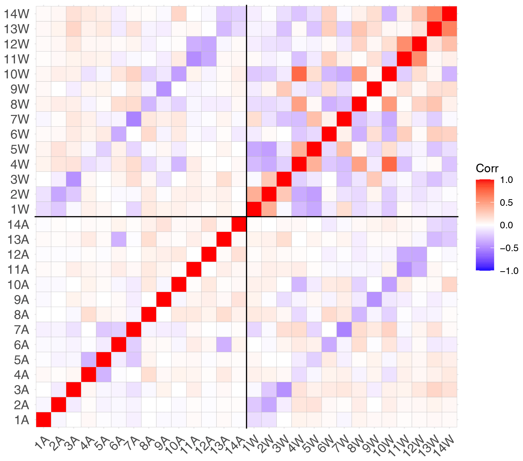
Figure 6Posterior error correlations between regional anthropogenic and wetland emissions. To examine error aliasing at a regional scale, anthropogenic emissions resolved on the grid are aggregated to the 14 subcontinental regions in Fig. 1 used for optimizing wetland emissions. Numbers (1–14) indicate the region index as in Fig. 1. “A” and “W” stand for anthropogenic and wetland emissions, respectively. For example, 5A stands for anthropogenic emissions from temperate North America.
4.1 Anthropogenic emissions
Figure 7 shows the correction factors from the inversion to 2010–2018 mean non-wetland emissions (posterior-to-prior ratios) along with the associated averaging kernel sensitivities (corresponding diagonal terms of the averaging kernel matrix). We achieve 179 independent pieces of information (DOFS) for constraining the emissions on the grid. The spatial distribution of averaging kernel sensitivities largely follows the pattern of prior emissions (right panel of Fig. 5). The inversion provides strong constraints in major anthropogenic source regions such as East Asia, South Asia, and South America. The constraints are generally weaker over North America, Europe, and Africa, indicating that the inversion provides more diffuse spatial information in these regions.
We find that the prior emission inventory significantly overestimates anthropogenic emissions in eastern China (Fig. 7). The posterior estimate of Chinese anthropogenic emissions (47±1 Tg a−1) is 30 % lower than the prior estimate (67 Tg a−1) and is also lower than the latest national report from China to the UNFCCC of 55 Tg a−1 for 2014 (Fig. 8). Based on the relative contribution of each sector in the prior inventory, we attribute ∼60 % of this downward correction to coal mining. The overestimation of anthropogenic emissions from China has been reported by previous global and regional GOSAT inversion studies using different EDGAR inventory versions as prior estimates (Monteil et al., 2013; Thompson et al., 2015; Turner et al., 2015; Maasakkers et al., 2019; Miller et al., 2019).
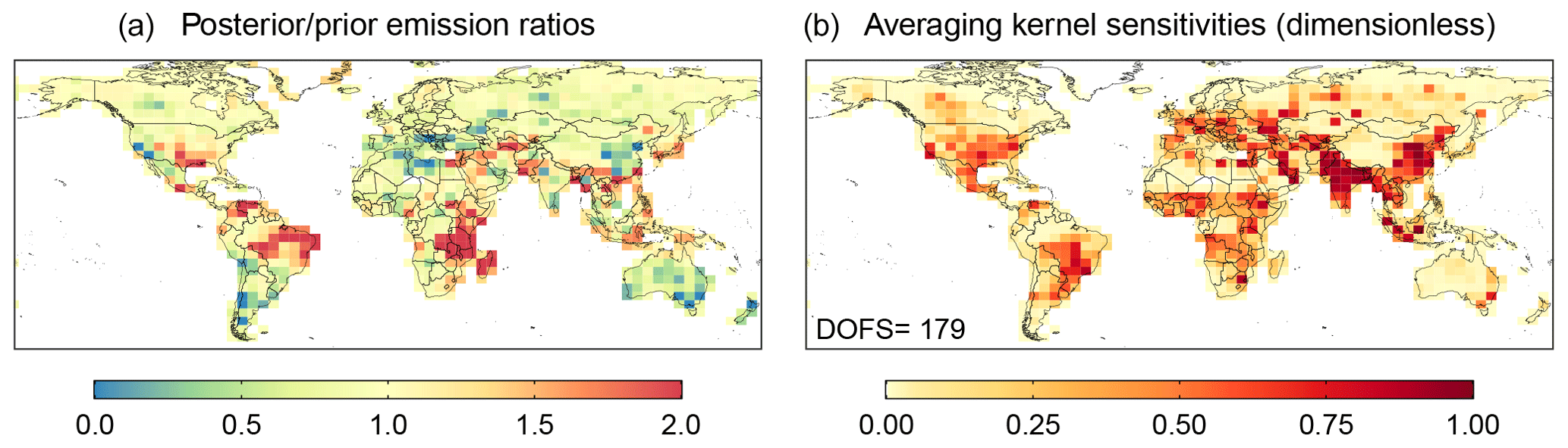
Figure 7Corrections to prior estimates of 2010–2018 mean non-wetland methane emissions. (a) Posterior-to-prior emission ratios. Figure S7 shows the same corrections as posterior–prior emission differences. (b) Averaging kernel sensitivities (diagonal elements of the averaging kernel matrix). The averaging kernel sensitivities measure the ability of the observations to constrain the posterior solution (0: not at all, 1: fully). The sum of averaging kernel sensitivities defines the degrees of freedom for signal (DOFS), which is inset.
Another major downward correction is for the oil- and gas-producing regions in Russia. We estimate Russia's anthropogenic emissions to be 20±1 Tg a−1 as opposed to the prior estimate of 34 Tg a−1 (Fig. 8), and the difference is mainly attributable to the oil and gas sector (posterior: 15 Tg a−1; prior: 27 Tg a−1). This finding is consistent with Maasakkers et al. (2019), though they used a different oil and gas emission inventory. Russia has been revising downwards its national emission estimates submitted to the UNFCCC, and our posterior estimate of total anthropogenic emissions is closer to the country's latest submission to the UNFCCC for 2010–2018 (16 Tg a−1; Fig. 8). The new submission revises oil and gas methane emissions downward by a factor of 3 relative to the previous submission used as a prior estimate in our inversion (Scarpelli et al., 2020).
We find large upward corrections to the prior inventory over East Africa (Mozambique, Zambia, Tanzania, Ethiopia, Uganda, Kenya, and Madagascar) and over South America (Brazil). A previous inversion suggested that corrections for these regions may be due to an underestimation of prior wetland emissions (Maasakkers et al., 2019). Our inversion, which optimizes wetland and anthropogenic emissions separately, attributes the underestimation to anthropogenic emissions (see also Sect. 4.3 for wetland results), though there is some error aliasing between them ( for sub-Saharan Africa, −0.4 for southern Africa; Fig. 6). We find that the upward correction over eastern Africa generally remains robust in a sensitivity inversion whereby prior wetland emissions in a neighboring region (Sudd in South Sudan) are increased by a factor of 3 (Figs. S4 and 8). Based on prior sectoral information, these underestimations are most likely due to livestock emissions, whose bottom-up estimates have large uncertainties in these developing regions (Herrero et al., 2013).
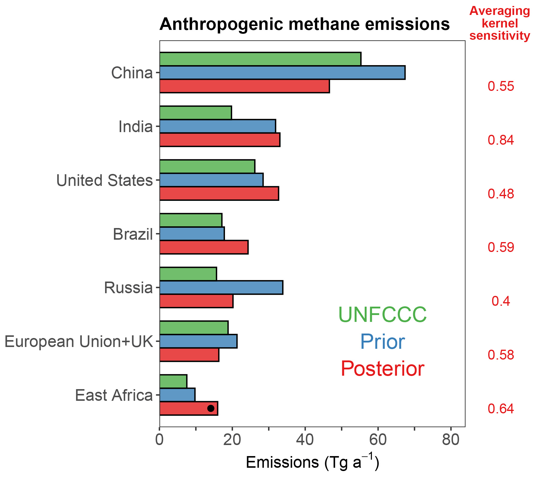
Figure 8National and regional estimates of 2010–2018 mean methane emissions from anthropogenic sources. Included are the top five individual countries in our posterior estimates, the European Union (including the United Kingdom), and East Africa (including Mozambique, Zambia, Tanzania, Ethiopia, Uganda, Kenya, and Madagascar). The UNFCCC record is from https://di.unfccc.int (last access: 10 July 2020). Non-Annex I countries do not report yearly emissions to the UNFCCC, and for those we use the latest UNFCCC submissions (Brazil, 2015; China, 2014; Ethiopia, 2013; India, Madagascar, Kenya, 2010; Uganda, Zambia, 2000; Mozambique, Tanzania, 1994). Inset are the averaging kernel sensitivities for these national and regional aggregated results, which measure the ability of the observations to constrain the posterior solution (0: not at all, 1: fully). The dot for East Africa represents the estimate inferred from a sensitivity inversion with the prior spatial distribution of African wetlands perturbed.
Another upward correction pattern in South America is located near Venezuela, a major oil-producing country in the region. The large correction in Venezuela likely reflects underestimation of fossil fuel emissions by the national estimates for 2010 reported to the UNFCCC. Upward corrections are also seen in central Asia (Iran, Turkmenistan), where the regional posterior estimates (10.1±0.9 Tg a−1) are 49 % higher than the prior (6.8 Tg a−1), with adjustments mainly attributed to the oil and gas sector. This region has previously been identified by satellite observations as a methane emission hot spot (Buchwitz et al., 2017; Varon et al., 2019; Schneising et al., 2020).
The inversion finds small upward corrections over the US (prior: 28 Tg a−1; posterior: 33±1 Tg a−1) (Fig. 8), resulting mainly from underestimation of emissions from the oil and gas sector in the western and south-central US (Fig. 7). This result is consistent with a high-resolution inversion over the US using the 2010–2015 GOSAT data, which spatially allocates the correction more specifically to oil and gas basins (Maasakkers et al., 2020). A number of previous studies have found that emissions from oil and gas production are underestimated in the national US inventory (e.g., Kort et al., 2014; Smith et al., 2017; Peischl et al., 2018; Alvarez et al., 2018; Y. Zhang et al., 2020; Gorchov Negron et al., 2020).
Small downward corrections with a diffuse pattern are found over Europe. The posterior estimate of anthropogenic emissions for the European Union (including the UK) is 16±0.7 Tg a−1, slightly lower than the prior estimate (21 Tg a−1) and the UNFCCC national reports (19 Tg a−1 for 2014) (Fig. 8). Source sector attribution is difficult in this case because of spatial overlap between emission sectors. The inversion finds only small adjustments to prior emissions for India (prior: 32 Tg a−1; posterior: 33±0.6 Tg a−1) even though the information content is relatively large, confirming the prior inventory used in the inversion. Our estimate, however, is much higher than a previous inversion study for India (Ganesan et al., 2017) (22 Tg a−1), the results of which are in agreement with India's UNFCCC report (20 Tg a−1 for 2010) (Fig. 8). Our inversion attributes the discrepancy with the UNFCCC submission mainly to the livestock sector.
4.2 Anthropogenic emission trends
Figure 9 shows the spatial distribution of 2010–2018 trends for anthropogenic emissions inferred from GOSAT observations, along with the associated averaging kernel matrix sensitivities. The GOSAT observations provide 42 pieces of information to constrain the spatial distribution of anthropogenic emission trends, suggesting that, compared to mean emissions, the inversion is only able to constrain more diffuse spatial patterns for emission trends. These constraints are strongest in China and India, but there is also fairly strong information aggregated over other continental regions. The prior estimate assumed zero anthropogenic trends anywhere; therefore, the posterior trends are driven solely by the GOSAT information.
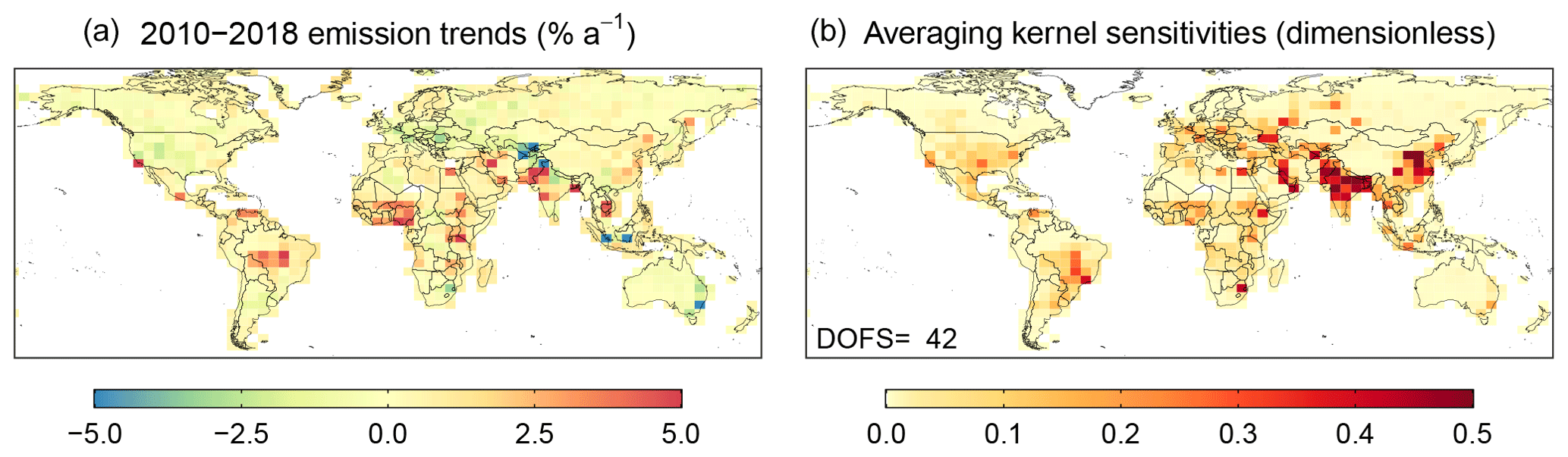
Figure 9Anthropogenic methane emission trends for 2010–2018, as informed by GOSAT observations. (a) Relative emission trends on the grid. Absolute emission trends are shown in Fig. S8. (b) Averaging kernel sensitivities that measure the ability of the observations to constrain the posterior solution (0: not at all, 1: fully). The degrees of freedom for signal (DOFS) are inset.
Significant positive trends of anthropogenic emissions are found in South Asia (0.58±0.16 Tg a−1 a−1 or 1.4±0.4 % a−1; Pakistan and India), East Africa (0.22±0.10 Tg a−1 a−1 or 1.4±0.6 % a−1; Ethiopia, Tanzania, Uganda, Kenya, and Sudan), West Africa (0.28±0.10 Tg a−1 a−1 or 4.4±1.4 % a−1; Nigeria, Niger, Ghana, Côte d'Ivoire, Mali, Benin, Burkina Faso), and Brazil (0.19±0.15 Tg a−1 a−1 or 0.8±0.6 % a−1). Based on prior sectoral fractions in each grid cell, we attribute these positive trends mostly to the livestock sector (0.31 Tg a−1 a−1 in South Asia, 0.13 Tg a−1 a−1 in East Africa, 0.09 Tg a−1 a−1 in West Africa, and 0.17 Tg a−1 a−1 in Brazil). Indeed, according to the United Nations Food and Agriculture Office (UNFAO) statistics (http://www.fao.org/faostat, last access: 22 June 2020), all these regions have had rapid increases in livestock population. The fastest-growing cattle populations in the world reported by the UNFAO over the 2010–2016 period were in Pakistan (1.4×10⁶ heads a−1), Ethiopia (1.2×10⁶ heads a−1), Tanzania (1.1×10⁶ heads a−1), and Brazil (0.9×10⁶ heads a−1). Moreover, our inversion results for these regional trends in livestock emissions are generally consistent in magnitude with the trends from bottom-up livestock emission inventories (FAOSTAT, IPCC tier I method; EDGAR v4.3.2 and v5, hybrid tier I method; Chang et al., 2019, IPCC tier II method) (Fig. 10). Because our inversion assumes zero prior trends in anthropogenic emissions, the inferred trends are solely informed by satellite observations and are independent of the bottom-up trends in Fig. 10.
A positive trend in anthropogenic emissions (0.39±0.27 Tg a−1 a−1 or 0.8±0.6 % a−1) is found over China driven by coal mining (northern China) and rice (southern China), but the magnitude of the trend is smaller than previous inverse analyses of satellite and surface observations for time horizons before 2015 (Bergamaschi et al., 2013; Thompson et al., 2015; Patra et al., 2016; Saunois et al., 2017; Miller et al., 2019; Maasakkers et al., 2019). We infer a much stronger trend (0.72±0.39 Tg a−1 a−1 or 1.6±0.9 % a−1) for China if we restrict the GOSAT record to 2010–2016. Our results thus suggest that anthropogenic emission trends in China peaked midway within the 2010–2018 record. Indeed, coal production in China peaked in 2013 (Sheng et al., 2019).
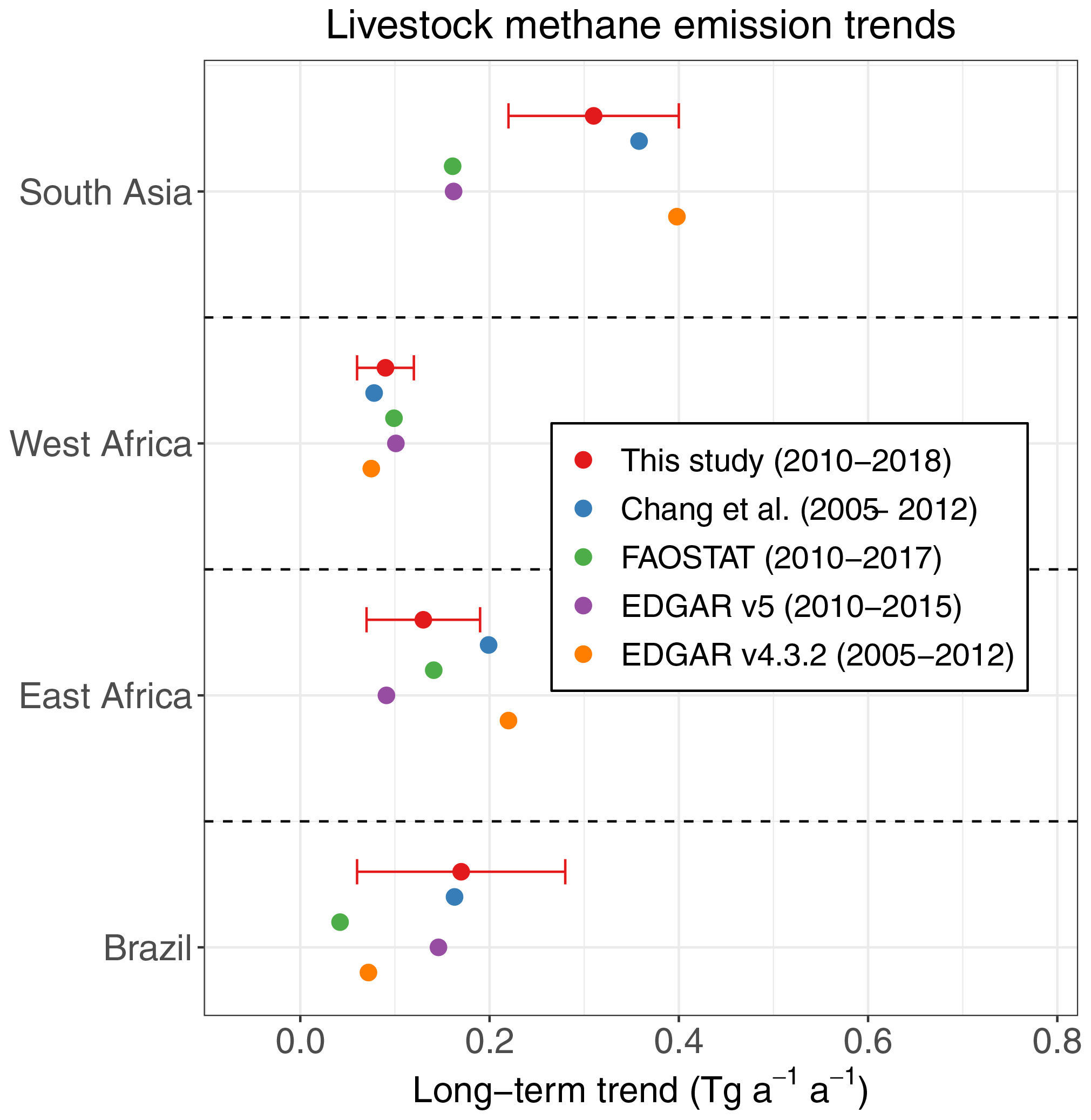
Figure 10Regional trends in anthropogenic methane emissions from livestock. Our GOSAT inversion results for 2010–2018 (with error standard deviations) are compared to estimates from different bottom-up inventories over the 2005–2017 period: Chang et al. (2019), FAOSTAT (2020), EDGAR v5 (Crippa et al., 2019), and EDGAR v4.3.2 (Janssens-Maenhout et al., 2017). Results are shown for South Asia (India and Pakistan), West Africa (Nigeria, Côte d'Ivoire, Mali, Niger, Burkina Faso, Cameroon, Ghana, and Benin), East Africa (Ethiopia, Kenya, Uganda, and Tanzania), and Brazil. By assuming zero prior trends in anthropogenic emissions, our inversion does not use trend information in any of these bottom-up inventories; the trends inferred by the inversion are solely from the GOSAT observations.
The inversion does not find significant 2010–2018 trends in anthropogenic emissions over the US ( Tg a−1 a−1, % a−1). This is generally consistent with the lack of a trend in US emissions over 2000–2014 in inversions collected by the Global Carbon Project (Bruhwiler et al., 2017) and over 2010–2015 in a North America regional inversion using GOSAT data (Maasakkers et al., 2020). It contradicts the 2 % a−1–3 % a−1 positive trend inferred from direct analysis of GOSAT enhancements (Turner et al., 2016; Sheng et al., 2018a) and the inference of large positive trends based on increasing concentrations of ethane and propane (Franco et al., 2016; Hausmann et al., 2016; Helmig et al., 2016). Bruhwiler et al. (2017) pointed out that the inference of methane emission trends from a simple analysis of GOSAT data could be subject to various biases including variability in background and seasonal sampling, which would be accounted for in an inversion. Increasing ethane-to-methane and propane-to-methane emission ratios over years may confound the inference of methane emission trends from ethane and propane records (Lan et al., 2019).
Small negative trends are found in central Asia (Uzbekistan, Kazakhstan, Turkmenistan, Afghanistan; Tg a−1 a−1), Europe ( Tg a−1 a−1), and Australia ( Tg a−1 a−1). The decrease in central Asia is attributed mainly to oil and gas, and the decrease in Australia is attributed to coal mining and livestock. Trends over Europe and Russia are too diffuse to be separated by sectors. No significant trend is found in Russia ( Tg a−1 a−1).
4.3 Wetland emissions
From the inversion we infer wetland emissions for 14 subcontinental regions (Fig. 1) and for individual months from 2010 to 2018, thus allowing seasonal and interannual variability to be optimized. This achieves 167 independent pieces of information (DOFS) for wetland emissions. The results are presented as mean seasonal cycles (Fig. 11) and time series of annual means (Fig. 12). Recent studies have found that the mean WetCHARTs inventory used here as a prior estimate is too high in the Congo Basin and too low in the Sudd region (Lunt et al., 2019; Parker et al., 2020b; Pandey et al., 2021). Our inversion is unable to resolve this subregional spatial correction pattern because of coarse resolution in the wetland state vector (Fig. 1). We therefore perform a sensitivity inversion with modified prior estimates following Lunt et al (2019) (Fig. S1), which finds a 20 % (3 Tg a−1) increase in estimates of the 2010–2018 average for sub-Saharan Africa and a 7 % (0.6 Tg a−1) increase for southern Africa relative to the base inversion (Fig. S5). Interannual trends and seasonal cycles are almost unchanged between the two inversions (Fig. S5).
As shown in Figs. 11 and 12, our results find lower wetland emissions than the mean of the WetCHARTs ensemble (prior estimate) over the Amazon, temperate North America (the US), and eastern Canada. The previous inversion of GOSAT data by Maasakkers et al. (2019) also found overestimation of emissions by WetCHARTs in the coastal US and Canadian wetlands but did not have significant corrections over the Amazon. The overestimation of wetland emissions in the US and eastern Canada is also reported in analyses of aircraft measurements in the southeastern US (Sheng et al., 2018b) and surface observations in Canada (Baray et al., 2021), both of which used WetCHARTs v1.0 as prior information. The downward correction of North American emissions is consistent with recent WetCHARTs updates (v1.2.1) that substantially reduce methane emissions across regions categorized as partial wetland complexes (Lehner and Döll, 2004; Bloom et al., 2017).
The seasonal cycles inferred from the inversion are in general consistent with prior information (Fig. 11), although averaging kernel sensitivities indicate that we only have limited constraints on the seasonality, particularly for high-latitude regions in Northern Hemisphere winter. This was generally expected given the limited GOSAT observational coverage at high latitudes during winter months. The inversion infers a sharp and late (May–June) onset of methane emissions across boreal wetlands, in contrast to an early and gradual increase starting from March predicted by the prior inventory. This feature in posterior estimates appears to be consistent with aircraft and surface observations over Canada's Hudson Bay Lowlands (Pickett-Heaps et al., 2011) and eddy flux measurements over Alaskan Arctic tundra (Zona et al., 2016), while the gradual onset in the prior inventory agrees with aircraft observations over Alaska by Miller et al. (2016). The negative fluxes right before the onset may reflect strong soil sinks during spring thaw over these high-latitude regions (Jørgensen et al., 2015). The inversion also indicates stronger seasonal cycles than the prior inventory in sub-Saharan Africa and tropical South Asia, which suggests that WetCHARTs may underestimate the sensitivity of wetland emissions to precipitation but overestimate their sensitivity to temperature.
Our posterior estimates of 2010–2018 trends in wetland emissions vary greatly by region and are generally larger than the prior estimates from WetCHARTs (Fig. 12). Large positive trends are found in the tropics (Amazon: +1.0 Tg a−1 a−1; sub-Saharan Africa: +0.6 Tg a−1 a−1; southern Africa: +0.4 Tg a−1 a−1) and high latitudes (Siberia: +0.4 Tg a−1 a−1). Increasing Amazonian wetland emissions may have been driven by intensification of flooding (Barichivich et al., 2018) or increasing temperature (Tunnicliffe et al., 2020) in the region over the past decades. Our result of increasing tropical Africa wetland emissions is consistent with a previous regional analysis of GOSAT data, which found a positive trend of 1.5–2.1 Tg a−1 a−1 in the region for 2010–2016 attributed mainly to wetlands, particularly the Sudd in South Sudan (Lunt et al., 2019). Compared to steady and linear increases in the tropics, boreal Siberia and northern Europe show abrupt increases in 2016–2018 for reasons that are unclear (Fig. 12). Decreasing but weaker trends are found in tropical Southeast Asia (−0.2 Tg a−1 a−1) and Australia (−0.1 Tg a−1 a−1).
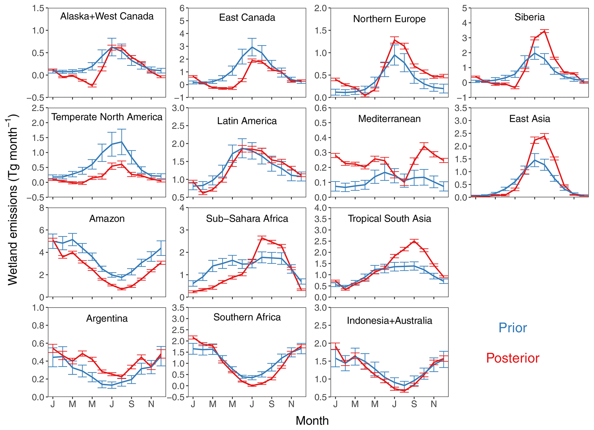
Figure 11Seasonal variation in wetland emissions for 14 subcontinental regions (Fig. 1). Values are means for 2010–2018. The prior estimate is the mean of the WetCHARTs inventory ensemble (Bloom et al., 2017). The posterior estimate is from our inversion of GOSAT data. Vertical bars are error standard deviations. The reduction of error in the posterior estimate measures the information content provided by the GOSAT data. Scales are different between panels.

Figure 12Wetland emission trends for 2010–2018. The figure shows annual mean emissions for the prior estimate (mean of WetCHARTs inventory ensemble) and the posterior estimate after inversion of GOSAT data. Values are for the 14 subcontinental regions in Fig. 1 (panels with a white background) and also aggregated for the extratropics and tropics (panels with a grey background). The trends are from ordinary linear regression. Inset are prior and posterior 2010–2018 average annual emissions (Tg a−1) with 2010–2018 trends (Tg a−1 a−1) in parentheses. Significant trends at the 95 % confidence level are denoted with *. Note the differences in scales between panels.
4.3.1 OH concentration
Our inversion infers a global methane lifetime against oxidation by tropospheric OH of 12.4±0.3 a, which is 15 % longer than the prior estimate (10.7±1.1 a) and is at the higher end of the inference from the methyl chloroform proxy (11.2±1.3 years) (Prather et al., 2012). We find that the downward correction for OH concentrations is mainly in the Northern Hemisphere. The north-to-south inter-hemispheric OH ratio is 1.02±0.05 in the posterior estimate compared to 1.16 in the prior estimate and 1.28±0.10 in the ACCMIP model ensemble (Naik et al., 2013). It is more consistent with the observation-based estimate of 0.97±0.12 (Patra et al., 2014). No significant 2010–2018 trend is seen in the methane lifetime (Fig. 13). The OH concentration in 2014 is 5 % lower than average, which may relate to particularly large peatland fires over Indonesia in 2014 that would be very large sources of carbon monoxide (CO) as a sink for OH (Pandey et al., 2017b).

Figure 13Methane loss frequency and lifetime against oxidation by tropospheric OH for 2010–2018. Values are annual means with error standard deviations. The loss frequency (k) is as calculated by Eq. (1) and the lifetime (τ) is the inverse. The prior estimate from Wecht et al. (2014) assumes no 2010–2018 trend in OH concentrations; the slight variability seen in the figure is due to temperature.
4.4 Attribution of the 2010–2018 methane trend
Figure 14 shows the 2010–2018 annual methane growth rates inferred from NOAA background surface measurements (Dlugokencky, 2020) and from our inversion of GOSAT data. There is general consistency between the two, with both showing the highest growth rates in 2014–2015 and a general acceleration after 2014. Our inversion achieves a much better match to the interannual variability of the NOAA record than the previous work of Maasakkers et al. (2019), in large part because of our optimization of the interannual variability of wetland emissions.
The bottom panel of Fig. 14 attributes the interannual variability in the methane growth rate to individual processes as determined by the inversion. The growth rate in year j (where m is the global methane mass) is determined by the balance between sources and sinks:
Here, Ej denotes the global emissions in year j, for which the inversion provides further sectoral breakdown, kj is the loss frequency against oxidation by tropospheric OH (Eq. 1), mj is the total methane mass, and Lj represents the minor sinks not optimized by the inversion. Let , , and represent the changes relative to 2010 conditions (Eo, ko, mo) taken as a reference. We can then write
where we have neglected the minor terms ΔkjΔmj and ΔLj. Here, the growth rate Gj in year j is decomposed into three terms: (1) a relaxation to steady state based on 2010 conditions (), (2) a perturbation to emissions (ΔEj) that can be further disaggregated by sectors, and (3) a perturbation to OH concentrations (moΔkj).
We see from the bottom panel of Fig. 14 that the legacy of the 2010 imbalance sustains a positive growth rate throughout the 2010–2018 period, but this influence diminishes towards the end of the record. The 2010–2018 trend in anthropogenic emissions is linear by design of the inversion and sustains a steady growth rate over the 2010–2018 period as the legacy of the 2010 imbalance declines. Figure 15 shows the sectoral breakdown of the anthropogenic trend. The increase in global anthropogenic emissions totalling 1.9±0.8 Tg a−1 a−1 is driven by livestock (0.70±0.36 Tg a−1 a−1; South Asia, tropical Africa, Brazil), rice (0.44±0.18 Tg a−1 a−1; East Asia), and wastewater treatment (0.33±0.13 Tg a−1 a−1; Asia). We find an insignificant positive global trend in emissions from fuel exploitation (oil, gas, and coal) (0.18±0.4 Tg a−1 a−1) (Fig. 15).
The bottom panel of Fig. 14 also shows that the spike in the methane growth rate in 2014–2015 is attributed to an anomalously low OH concentration in 2014 (5 % lower than 2010–2018 average; Fig. 13), partly offset by low wetland emissions and anomalously high fire emissions in 2015, mostly from Indonesia peatlands (Worden et al., 2017). Smoldering peatland fires are particularly large sources of methane (Liu et al., 2020). The large fire emissions are informed by the GFED inventory because the interannual variability of fire emissions is not optimized in our inversion. Despite their small magnitude relative to wetland and anthropogenic emissions globally, anomalous fire emissions can be an important contributor to methane interannual variability (Worden et al., 2017; Pandey et al., 2017b) both directly by releasing methane and indirectly by decreasing OH concentrations through CO emissions.
In addition to the 2014–2015 extremum, the NOAA surface observations show an acceleration of methane growth during the latter part of the 2010–2018 record (Nisbet et al., 2019), and this is reproduced in our inversion (Fig. 14). This accelerating growth is driven by strong wetland emissions, particularly in 2016–2018, on top of increasing anthropogenic emissions (Fig. 14). Our inversion infers a relatively steady 2010–2018 increase from tropical wetlands (in particular the Amazon and tropical Africa) and a 2016–2018 surge from extratropical wetlands (in particular boreal Eurasia) (Fig. 12). More work is needed to understand the drivers of changes in wetland emissions.
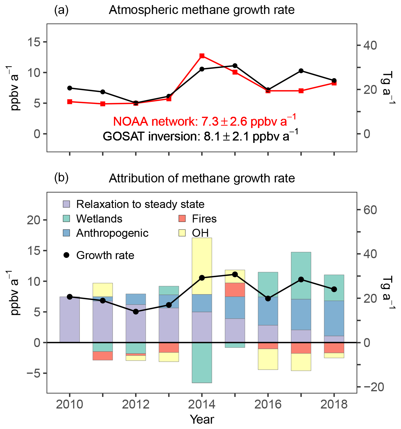
Figure 14The 2010–2018 annual growth rates in global atmospheric methane. (a) Comparison of annual growth rates inferred from our inversion of GOSAT data and from the NOAA surface network (Dlugokencky, 2020). Average methane growth rates for the period are inset. (b) Attribution of annual growth rates in the GOSAT inversion to perturbations of emissions (anthropogenic, wetlands, fires) and OH concentrations relative to 2010 conditions. The purple bar shows the relaxation of the 2010 budget imbalance to steady state. See the text for details explaining the breakdown.
We estimate from the inversion global mean methane emissions for 2010–2018 of 512±4 Tg a−1 (wetlands: 145 Tg a−1; anthropogenic: 336 Tg a−1) and a sink of 489±4 Tg a−1. This posterior global emission is lower than the prior estimate (538 Tg a−1) and the 538–593 Tg a−1 range reported by the Global Carbon Project for 2008–2017 (Saunois et al., 2020). Compared to prior emissions, we estimate lower emissions for wetlands and fossil fuel and higher emissions for livestock and rice (Figs. 12 and 15). Meanwhile, we estimate a methane lifetime against tropospheric OH oxidation of 12.4±0.3 years, which is at the high end of 11.2±1.3 years based on the methyl chloroform proxy (Prather et al., 2012), though strong error correlations between wetland emissions and methane lifetime suggest that our inversion has limited ability to constrain both independently (Fig. 5).
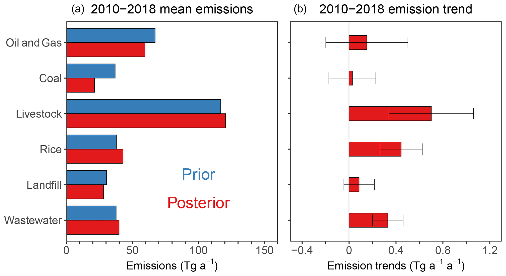
Figure 15The 2010–2018 global methane anthropogenic emissions and emission trends partitioned by individual sectors. Posterior estimates are from our inversion of GOSAT data. Prior estimates for anthropogenic emission trends are zero. Error bars in (b) show posterior error standard deviations for emission trends. Posterior error standard deviations for mean emissions are small and are thus not shown in (a).
We quantified the regional and sectoral contributions to global atmospheric methane and its 2010–2018 trend through the inversion of GOSAT observations. The inversion jointly optimizes (1) 2010–2018 anthropogenic emissions and their linear trends on a grid, (2) wetland emissions in 14 subcontinental regions for individual months, and (3) annual mean hemispheric OH concentrations for individual years. An analytical solution to the optimization problem provides closed-form estimates of posterior error covariances and information content, allowing us in particular to diagnose error correlations in our solution. The separate optimization of wetland and anthropogenic emissions allows us to resolve interannual and seasonal variations in posterior wetland emissions. Our inversion introduces additional innovations, including the correction of stratospheric model biases using ACE-FTS satellite data, and a new bottom-up inventory for emissions from fossil fuel exploitation based on national reports to the UNFCCC (Scarpelli et al., 2020).
Our optimization of 2010–2018 mean anthropogenic emissions on the grid provides strong information in source regions as measured by averaging kernel sensitivities. We find that estimates of anthropogenic emissions reported by individual countries to the UNFCCC are too high for China (coal emissions) and Russia (oil and gas emissions) and too low for Venezuela (oil and gas) and the US (oil and gas). We also find that tropical livestock emissions are larger than previous estimates, particularly in South Asia, Africa, and Brazil. Our posterior estimate of anthropogenic emissions in India (33 Tg a−1) is much higher than its most recent (2010) report to the UNFCCC (20 Tg a−1), mostly because of livestock emissions.
The 2010–2018 trends in methane emissions on the grid are successfully quantified in source regions. We find that large growth in anthropogenic emissions occurs in tropical regions including South Asia, tropical Africa, and Brazil that can be attributed to the livestock sector. This finding is consistent with trends in livestock populations. There has been little discussion in the literature about increasing agricultural methane emissions in these developing countries (Jackson et al., 2020). Our results also show a 2010–2018 increase in Chinese emissions, but the inferred rate of the increase is smaller than previously reported in inversions focused on earlier periods, likely caused by leveling of coal emissions in China. The 2010–2018 emission trend in the US is insignificant on the national scale.
We find that global wetland emissions are lower than the mean WetCHARTs emissions used as a prior estimate, mostly because of the Amazon. Wetland emissions over North America are also lower, consistent with previous studies. In both cases, posterior estimates are all well within the full WetCHARTs uncertainty range (Bloom et al., 2017). The seasonality of wetland emissions inferred by the inversion is in general consistent with WetCHARTs. An exception is in boreal wetlands where we find negative fluxes in April–May, possibly reflecting methane uptake as the soil thaws. The inversion infers increasing wetland emissions over the 2010–2018 period, superimposed on large interannual variability, in both the tropics (the Amazon, tropical Africa) and extratropics (Siberia).
Our optimization of annual hemispheric OH concentrations yields a global methane lifetime of 12.4±0.3 years against oxidation by tropospheric OH, with an inter-hemispheric OH ratio of 1.02. Our best estimate is that the global OH concentration has no significant trend over 2010–2018 except for a 5 % dip in 2014.
Taking all these methane budget terms together, our inversion of GOSAT data estimates global mean methane emissions for 2010–2018 of 512 Tg a−1, with 336 Tg a−1 from anthropogenic sources, 145 Tg a−1 from wetland sources, and 31 Tg a−1 from other natural sources. Our inferred growth rate of methane over that period matches that observed at NOAA background sites, including peak growth rates in 2014–2015 and an overall acceleration over the 2010–2018 period. We attribute the 2014–2015 peaks in methane growth rates to low OH concentrations (2014) and high fire emissions (2015), and we attribute the overall acceleration to a sustained increase in anthropogenic emissions over the period and strong wetland emissions in the latter part of the period. Most of the increase in anthropogenic emissions is attributed to livestock (in tropics), with contributions from increases in rice and wastewater emissions (Asia). Our best estimate indicates a positive trend from fuel exploitation, but this trend is statistically insignificant given the uncertainty of the inversion. Our finding is in general consistent with a previous 2010–2015 inversion of GOSAT data (Maasakkers et al., 2019), although here we use a longer record and capture the interannual variability better. Our results also agree with isotopic data, indicating that the rise in methane is driven by biogenic sources (Schaefer et al., 2016; Nisbet et al., 2016). The increase in tropical livestock emissions is quantitatively consistent with bottom-up estimates. More work is needed to understand interannual variations in wetland emissions.
The dataset for the 2010–2018 global inversion results is archived (https://doi.org/10.5281/zenodo.4052518; Zhang et al., 2021). The GOSAT proxy satellite methane observations are available at the CEDA archive (https://doi.org/10.5285/18ef8247f52a4cb6a14013f8235cc1eb, Parker and Boesch, 2020). The ACE-FTS satellite observations can be requested through http://www.ace.uwaterloo.ca/data.php (ACE, 2020). TCCON data were obtained from the TCCON Data Archive hosted by CaltechDATA (https://tccondata.org) (Deutscher et al., 2017; Dubey et al., 2017; Feist et al., 2017; Goo et al., 2017; Griffith et al., 2017a, b; Hase et al., 2017; Iraci et al., 2017a, b; Kivi et al., 2017; Liu et al., 2018; de Maziere et al., 2017; Morino et al., 2017a, b, c; Notholt et al., 2019a, b; Sherlock et al., 2017a, b; Shiomi et al., 2017; Strong et al., 2017; Sussmann et al., 2017; Te et al., 2017; Warneke et al., 2017; Wennberg et al., 2017a, b, c, d; Wunch et al., 2017). NOAA surface observations are accessed through the NOAA ESRL/GMD CCGG Group (https://doi.org/10.15138/VNCZ-M766) (Dlugokencky et al., 2020). National reports to the UNFCCC are available through the UNFCCC's Greenhouse Gas Inventory Data Interface (https://di.unfccc.int/detailed_data_by_party, UNFCCC, 2020). EDGAR anthropogenic emission inventories (v4.3.2 and v5) are available at https://data.europa.eu/doi/10.2904/JRC_DATASET_EDGAR (European Commission, 2020).
The supplement related to this article is available online at: https://doi.org/10.5194/acp-21-3643-2021-supplement.
YZ and DJJ designed the study. YZ conducted the modeling and data analyses with contributions from XL, JDM, TRS, MPS, JXS, LS, and ZQ. RJP and HB provided the GOSAT methane retrievals. AAB and SM contributed to the WetCHARTs wetland emission inventory and its interpretation. JC contributed to analyses and interpretation of bottom-up livestock emission inventories. YZ and DJJ wrote the paper with inputs from all authors.
The authors declare that they have no conflict of interest.
Work at Harvard was supported by the NASA Carbon Monitoring System (CMS), Interdisciplinary Science (IDS), and Advanced Information Systems Technology (AIST) programs. Yuzhong Zhang was supported by Harvard University, the Kravis Fellowship through the Environmental Defense Fund (EDF), the National Natural Science Foundation of China (project: 42007198), and the foundation of Westlake University. Yuzhong Zhang thanks Peter Bernath and Chris Boone for discussion on the ACE-FTS data and Benjamin Poulter for discussion on attribution of the atmospheric methane trend. Part of this research was carried out at the Jet Propulsion Laboratory, California Institute of Technology, under a contract with NASA. Robert J. Parker and Hartmut Boesch are funded via the UK National Centre for Earth Observation (NE/R016518/1 and NE/N018079/1). Robert J. Parker and Hartmut Boesch also acknowledge funding from the ESA GHG-CCI and Copernicus C3S projects. We thank the Japanese Aerospace Exploration Agency, the National Institute for Environmental Studies, and the Ministry of Environment for the GOSAT data and their continuous support as part of a joint research agreement. GOSAT retrievals were performed with the ALICE high-performance computing facility at the University of Leicester.
This research has been supported by NASA (grant nos. 80NSSC18K0178, NNX17AK81G, 80NSSC20K0009, and 1647811), the NSFC (42007198), and the UK National Centre for Earth Observation (NE/R016518/1 and NE/N018079/1).
This paper was edited by Bryan N. Duncan and reviewed by two anonymous referees.
ACE Atmospheric Chemistry Experiment: ACE-FTS satellite observations, available at: http://www.ace.uwaterloo.ca/data.php, last access: 20 July 2020.
Alexe, M., Bergamaschi, P., Segers, A., Detmers, R., Butz, A., Hasekamp, O., Guerlet, S., Parker, R., Boesch, H., Frankenberg, C., Scheepmaker, R. A., Dlugokencky, E., Sweeney, C., Wofsy, S. C., and Kort, E. A.: Inverse modelling of CH4 emissions for 2010–2011 using different satellite retrieval products from GOSAT and SCIAMACHY, Atmos. Chem. Phys., 15, 113–133, https://doi.org/10.5194/acp-15-113-2015, 2015.
Alvarez, R. A., Zavala-Araiza, D., Lyon, D. R., Allen, D. T., Barkley, Z. R., Brandt, A. R., Davis, K. J., Herndon, S. C., Jacob, D. J., Karion, A., Kort, E. A., Lamb, B. K., Lauvaux, T., Maasakkers, J. D., Marchese, A. J., Omara, M., Pacala, S. W., Peischl, J., Robinson, A. L., Shepson, P. B., Sweeney, C., Townsend-Small, A., Wofsy, S. C., and Hamburg, S. P.: Assessment of methane emissions from the U.S. oil and gas supply chain, Science, 361, 186–188, https://doi.org/10.1126/science.aar7204, 2018.
Baray, S., Jacob, D. J., Massakkers, J. D., Sheng, J.-X., Sulprizio, M. P., Jones, D. B. A., Bloom, A. A., and McLaren, R.: Estimating 2010–2015 Anthropogenic and Natural Methane Emissions in Canada using ECCC Surface and GOSAT Satellite Observations, Atmos. Chem. Phys. Discuss. [preprint], https://doi.org/10.5194/acp-2020-1195, in review, 2021.
Barichivich, J., Gloor, E., Peylin, P., Brienen, R. J. W., Schöngart, J., Espinoza, J. C., and Pattnayak, K. C.: Recent intensification of Amazon flooding extremes driven by strengthened Walker circulation, Sci. Adv., 4, eaat8785, https://doi.org/10.1126/sciadv.aat8785, 2018.
Bergamaschi, P., Houweling, S., Segers, A., Krol, M., Frankenberg, C., Scheepmaker, R. A., Dlugokencky, E., Wofsy, S. C., Kort, E. A., Sweeney, C., Schuck, T., Brenninkmeijer, C., Chen, H., Beck, V., and Gerbig, C.: Atmospheric CH4 in the first decade of the 21st century: Inverse modeling analysis using SCIAMACHY satellite retrievals and NOAA surface measurements, J. Geophys. Res.-Atmos., 118, 7350–7369, https://doi.org/10.1002/jgrd.50480, 2013.
Bernath, P. F., McElroy, C. T., Abrams, M. C., Boone, C. D., Butler, M., Camy-Peyret, C., Carleer, M., Clerbaux, C., Coheur, P.-F., Colin, R., DeCola, P., DeMazière, M., Drummond, J. R., Dufour, D., Evans, W. F. J., Fast, H., Fussen, D., Gilbert, K., Jennings, D. E., Llewellyn, E. J., Lowe, R. P., Mahieu, E., McConnell, J. C., McHugh, M., McLeod, S. D., Michaud, R., Midwinter, C., Nassar, R., Nichitiu, F., Nowlan, C., Rinsland, C. P., Rochon, Y. J., Rowlands, N., Semeniuk, K., Simon, P., Skelton, R., Sloan, J. J., Soucy, M.-A., Strong, K., Tremblay, P., Turnbull, D., Walker, K. A., Walkty, I., Wardle, D. A., Wehrle, V., Zander, R., and Zou, J.: Atmospheric Chemistry Experiment (ACE): Mission overview, Geophys. Res. Lett., 32, L15S01, https://doi.org/10.1029/2005gl022386, 2005.
Bloom, A. A., Bowman, K. W., Lee, M., Turner, A. J., Schroeder, R., Worden, J. R., Weidner, R., McDonald, K. C., and Jacob, D. J.: A global wetland methane emissions and uncertainty dataset for atmospheric chemical transport models (WetCHARTs version 1.0), Geosci. Model Dev., 10, 2141–2156, https://doi.org/10.5194/gmd-10-2141-2017, 2017.
Bousquet, P., Hauglustaine, D. A., Peylin, P., Carouge, C., and Ciais, P.: Two decades of OH variability as inferred by an inversion of atmospheric transport and chemistry of methyl chloroform, Atmos. Chem. Phys., 5, 2635–2656, https://doi.org/10.5194/acp-5-2635-2005, 2005.
Brasseur, G. P. and Jacob, D. J.: Modeling of Atmospheric Chemistry, Cambridge University Press, Cambridge, UK, 2017.
Bruhwiler, L. M., Basu, S., Bergamaschi, P., Bousquet, P., Dlugokencky, E., Houweling, S., Ishizawa, M., Kim, H.-S., Locatelli, R., Maksyutov, S., Montzka, S., Pandey, S., Patra, P. K., Petron, G., Saunois, M., Sweeney, C., Schwietzke, S., Tans, P., and Weatherhead, E. C.: U.S. CH4 emissions from oil and gas production: Have recent large increases been detected?, J. Geophys. Res.-Atmos., 122, 4070–4083, https://doi.org/10.1002/2016jd026157, 2017.
Buchwitz, M., Reuter, M., Schneising, O., Boesch, H., Guerlet, S., Dils, B., Aben, I., Armante, R., Bergamaschi, P., Blumenstock, T., Bovensmann, H., Brunner, D., Buchmann, B., Burrows, J. P., Butz, A., Chédin, A., Chevallier, F., Crevoisier, C. D., Deutscher, N. M., Frankenberg, C., Hase, F., Hasekamp, O. P., Heymann, J., Kaminski, T., Laeng, A., Lichtenberg, G., De Mazière, M., Noël, S., Notholt, J., Orphal, J., Popp, C., Parker, R., Scholze, M., Sussmann, R., Stiller, G. P., Warneke, T., Zehner, C., Bril, A., Crisp, D., Griffith, D. W. T., Kuze, A., O'Dell, C., Oshchepkov, S., Sherlock, V., Suto, H., Wennberg, P., Wunch, D., Yokota, T., and Yoshida, Y.: The Greenhouse Gas Climate Change Initiative (GHG-CCI): Comparison and quality assessment of near-surface-sensitive satellite-derived CO2 and CH4 global data sets, Remote Sens. Environ., 162, 344–362, https://doi.org/10.1016/j.rse.2013.04.024, 2015.
Buchwitz, M., Schneising, O., Reuter, M., Heymann, J., Krautwurst, S., Bovensmann, H., Burrows, J. P., Boesch, H., Parker, R. J., Somkuti, P., Detmers, R. G., Hasekamp, O. P., Aben, I., Butz, A., Frankenberg, C., and Turner, A. J.: Satellite-derived methane hotspot emission estimates using a fast data-driven method, Atmos. Chem. Phys., 17, 5751–5774, https://doi.org/10.5194/acp-17-5751-2017, 2017.
Burkholder, J. B., Sander, S. P., Abbatt, J., Barker, J. R., Huie, R. E., Kolb, C. E., Kurylo, M. J., Orkin, V. L., Wilmouth, D. M., and Wine, P. H.: Chemical Kinetics and Photochemical Data for Use in Atmospheric Studies, Evaluation No. 18, Jet Propulsion Laboratory, Pasadena, USA, 1392 pp., 2015.
Butchart, N. and Remsberg, E. E.: The Area of the Stratospheric Polar Vortex as a Diagnostic for Tracer Transport on an Isentropic Surface, J. Atmos. Sci., 43, 1319–1339, https://doi.org/10.1175/1520-0469(1986)043<1319:Taotsp>2.0.Co;2, 1986.
Chang, J., Peng, S., Ciais, P., Saunois, M., Dangal, S. R. S., Herrero, M., Havlík, P., Tian, H., and Bousquet, P.: Revisiting enteric methane emissions from domestic ruminants and their δ13C source signature, Nat. Commun., 10, 3420, https://doi.org/10.1038/s41467-019-11066-3, 2019.
Cressot, C., Chevallier, F., Bousquet, P., Crevoisier, C., Dlugokencky, E. J., Fortems-Cheiney, A., Frankenberg, C., Parker, R., Pison, I., Scheepmaker, R. A., Montzka, S. A., Krummel, P. B., Steele, L. P., and Langenfelds, R. L.: On the consistency between global and regional methane emissions inferred from SCIAMACHY, TANSO-FTS, IASI and surface measurements, Atmos. Chem. Phys., 14, 577–592, https://doi.org/10.5194/acp-14-577-2014, 2014.
Crippa, M., Oreggioni, G., Guizzardi, D., Muntean, M., Schaaf, E., Lo Vullo, E., Solazzo, E., Monforti-Ferrario, F., Olivier, J. G. J., and Vignati, E.: Fossil CO2 and GHG emissions of all world countries, 2019 Report, EUR 29849 EN, Publications Office of the European Union, Luxembourg, Luxemburg, 246 pp., https://doi.org/10.2760/687800, 2019.
de Maziere, M., Sha, M. K., Desmet, F., Hermans, C., Scolas, F., Kumps, N., Metzger, J.-M., Duflot, V., and Cammas, J.-P.: TCCON data from Reunion Island (La Reunion), France, Release GGG2014R0, TCCON data archive, CaltechDATA, https://doi.org/10.14291/tccon.ggg2014.reunion01.R1, 2017.
Deutscher, N. M., Notholt, J., Messerschmidt, J., Weinzierl, C., Warneke, T., Petri, C., Grupe, P., and Katrynski, K.: TCCON data from Bialystok, Poland, Release GGG2014R2, TCCON data archive, CaltechDATA, https://doi.org/10.14291/tccon.ggg2014.bialystok01.R2, 2017.
Dlugokencky, E. J., NOAA/GML: Trends in Atmospheric Methane: available at: https://www.esrl.noaa.gov/gmd/ccgg/trends_ch4/, last access: 22 June 2020.
Dlugokencky, E. J., Crotwell, A. M., Mund, J. W., Crotwell, M. J., and Thoning, K. W.: Atmospheric Methane Dry Air Mole Fractions from the NOAA GML Carbon Cycle Cooperative Global Air Sampling Network, Version 2020-07, https://doi.org/10.15138/VNCZ-M766, 2020.
Dubey, M., Henderson, B., Green, D., Butterfield, Z., Keppel-Aleks, G., Allen, N., Blavier, J. F., Roehl, C., Wunch, D., and Lindenmaier, R.: TCCON data from Manaus, Brazil, Release GGG2014R0, TCCON data archive, CaltechDATA, https://doi.org/10.14291/tccon.ggg2014.manaus01.R0/1149274, 2017.
Engel, A., Bönisch, H., Brunner, D., Fischer, H., Franke, H., Günther, G., Gurk, C., Hegglin, M., Hoor, P., Königstedt, R., Krebsbach, M., Maser, R., Parchatka, U., Peter, T., Schell, D., Schiller, C., Schmidt, U., Spelten, N., Szabo, T., Weers, U., Wernli, H., Wetter, T., and Wirth, V.: Highly resolved observations of trace gases in the lowermost stratosphere and upper troposphere from the Spurt project: an overview, Atmos. Chem. Phys., 6, 283–301, https://doi.org/10.5194/acp-6-283-2006, 2006.
Etiope, G., Ciotoli, G., Schwietzke, S., and Schoell, M.: Gridded maps of geological methane emissions and their isotopic signature, Earth Syst. Sci. Data, 11, 1–22, https://doi.org/10.5194/essd-11-1-2019, 2019.
European Commission: EDGAR anthropogenic emission inventories (v4.3.2 and v5), available at: https://data.europa.eu/doi/10.2904/JRC_DATASET_EDGAR, last access: 20 July 2020.
FAOSTAT Online Statistical Service (Food and Agriculture Organization, FAO): available at: http://faostat3.fao.org, last access: 20 January 2020.
Feist, D. G., Arnold, S. G., John, N., and Geibel, M. C.: TCCON data from Ascension Island, Saint Helena, Ascension and Tristan da Cunha, Release GGG2014R0, TCCON data archive, CaltechDATA, https://doi.org/10.14291/tccon.ggg2014.ascension01.R0/114928 5, 2017.
Franco, B., Mahieu, E., Emmons, L. K., Tzompa-Sosa, Z. A., Fischer, E. V., Sudo, K., Bovy, B., Conway, S., Griffin, D., Hannigan, J. W., Strong, K., and Walker, K. A.: Evaluating ethane and methane emissions associated with the development of oil and natural gas extraction in North America, Environ. Res. Lett., 11, 044010, https://doi.org/10.1088/1748-9326/11/4/044010, 2016.
Fraser, A., Palmer, P. I., Feng, L., Boesch, H., Cogan, A., Parker, R., Dlugokencky, E. J., Fraser, P. J., Krummel, P. B., Langenfelds, R. L., O'Doherty, S., Prinn, R. G., Steele, L. P., van der Schoot, M., and Weiss, R. F.: Estimating regional methane surface fluxes: the relative importance of surface and GOSAT mole fraction measurements, Atmos. Chem. Phys., 13, 5697–5713, https://doi.org/10.5194/acp-13-5697-2013, 2013.
Fung, I., John, J., Lerner, J., Matthews, E., Prather, M., Steele, L. P., and Fraser, P. J.: Three-dimensional model synthesis of the global methane cycle, J. Geophys. Res.-Atmos., 96, 13033–13065, https://doi.org/10.1029/91jd01247, 1991.
Ganesan, A. L., Rigby, M., Lunt, M. F., Parker, R. J., Boesch, H., Goulding, N., Umezawa, T., Zahn, A., Chatterjee, A., Prinn, R. G., Tiwari, Y. K., van der Schoot, M., and Krummel, P. B.: Atmospheric observations show accurate reporting and little growth in India's methane emissions, Nat. Commun., 8, 836, https://doi.org/10.1038/s41467-017-00994-7, 2017.
Gelaro, R., McCarty, W., Suárez, M. J., Todling, R., Molod, A., Takacs, L., Randles, C. A., Darmenov, A., Bosilovich, M. G., Reichle, R., Wargan, K., Coy, L., Cullather, R., Draper, C., Akella, S., Buchard, V., Conaty, A., Silva, A. M. D., Gu, W., Kim, G.-K., Koster, R., Lucchesi, R., Merkova, D., Nielsen, J. E., Partyka, G., Pawson, S., Putman, W., Rienecker, M., Schubert, S. D., Sienkiewicz, M., and Zhao, B.: The Modern-Era Retrospective Analysis for Research and Applications, Version 2 (MERRA-2), J. Climate, 30, 5419–5454, https://doi.org/10.1175/jcli-d-16-0758.1, 2017.
Goo, T. Y., Oh, Y. S., and Velazco, V. A.: TCCON data from Anmyeondo, South Korea, Release GGG2014R0, TCCON data archive, CaltechDATA, https://doi.org/10.14291/tccon.ggg2014.anmeyondo01.R0/1149 284, 2017.
Gorchov Negron, A. M., Kort, E. A., Conley, S. A., and Smith, M. L.: Airborne Assessment of Methane Emissions from Offshore Platforms in the U.S. Gulf of Mexico, Environ. Sci. Technol., 54, 5112–5120, https://doi.org/10.1021/acs.est.0c00179, 2020.
Griffith, D. W. T., Deutscher, N. M., Velazco, V. A., Wennberg, P. O., Yavin, Y., Keppel-Aleks, G., Washenfelder, R. A., Toon, G. C., Blavier, J. F., Murphy, C., Jones, N., Kettlewell, G., Connor, B. J., Macatangay, R., Roehl, C., Ryczek, M., Glowacki, J., Culgan, T., and Bryant, G.: TCCON data from Darwin, Australia, Release GGG2014R0, TCCON data archive, CaltechDATA, https://doi.org/10.14291/tccon.ggg2014.darwin01.R0/1149290, 2017a.
Griffith, D. W. T., Velazco, V. A., Deutscher, N. M., Murphy, C., Jones, N., Wilson, S., Macatangay, R., Kettlewell, G., Buchholz, R. R., and Riggenbach, M.: TCCON data from Wollongong, Australia, Release GGG2014R0, TCCON data archive, CaltechDATA, https://doi.org/10.14291/tccon.ggg2014.wollongong01.R0/1149 291, 2017b.
Gromov, S., Brenninkmeijer, C. A. M., and Jöckel, P.: A very limited role of tropospheric chlorine as a sink of the greenhouse gas methane, Atmos. Chem. Phys., 18, 9831–9843, https://doi.org/10.5194/acp-18-9831-2018, 2018.
Hase, F., Blumenstock, T., Dohe, S., Gross, J., and Kiel, M.: TCCON data from Karlsruhe, Germany, Release GGG2014R1, TCCON data archive, CaltechDATA, https://doi.org/10.14291/tccon.ggg2014.karlsruhe01.R1/1182416, 2017.
Hausmann, P., Sussmann, R., and Smale, D.: Contribution of oil and natural gas production to renewed increase in atmospheric methane (2007–2014): top–down estimate from ethane and methane column observations, Atmos. Chem. Phys., 16, 3227–3244, https://doi.org/10.5194/acp-16-3227-2016, 2016.
Heald, C. L., Jacob, D. J., Jones, D. B. A., Palmer, P. I., Logan, J. A., Streets, D. G., Sachse, G. W., Gille, J. C., Hoffman, R. N., and Nehrkorn, T.: Comparative inverse analysis of satellite (MOPITT) and aircraft (TRACE-P) observations to estimate Asian sources of carbon monoxide, J. Geophys. Res.-Atmos., 109, D23306, https://doi.org/10.1029/2004JD005185, 2004.
Hegglin, M. I., Brunner, D., Peter, T., Hoor, P., Fischer, H., Staehelin, J., Krebsbach, M., Schiller, C., Parchatka, U., and Weers, U.: Measurements of NO, NOy, N2O, and O3 during SPURT: implications for transport and chemistry in the lowermost stratosphere, Atmos. Chem. Phys., 6, 1331–1350, https://doi.org/10.5194/acp-6-1331-2006, 2006.
Helmig, D., Rossabi, S., Hueber, J., Tans, P., Montzka, S. A., Masarie, K., Thoning, K., Plass-Duelmer, C., Claude, A., Carpenter, L. J., Lewis, A. C., Punjabi, S., Reimann, S., Vollmer, M. K., Steinbrecher, R., Hannigan, J. W., Emmons, L. K., Mahieu, E., Franco, B., Smale, D., and Pozzer, A.: Reversal of global atmospheric ethane and propane trends largely due to US oil and natural gas production, Nat. Geosci., 9, 490–495, https://doi.org/10.1038/ngeo2721, 2016.
Herrero, M., Havlík, P., Valin, H., Notenbaert, A., Rufino, M. C., Thornton, P. K., Blümmel, M., Weiss, F., Grace, D., and Obersteiner, M.: Biomass use, production, feed efficiencies, and greenhouse gas emissions from global livestock systems, P. Natl. Acad. Sci. USA, 110, 20888–20893, https://doi.org/10.1073/pnas.1308149110, 2013.
Hmiel, B., Petrenko, V. V., Dyonisius, M. N., Buizert, C., Smith, A. M., Place, P. F., Harth, C., Beaudette, R., Hua, Q., Yang, B., Vimont, I., Michel, S. E., Severinghaus, J. P., Etheridge, D., Bromley, T., Schmitt, J., Faïn, X., Weiss, R. F., and Dlugokencky, E.: Preindustrial 14CH4 indicates greater anthropogenic fossil CH4 emissions, Nature, 578, 409–412, https://doi.org/10.1038/s41586-020-1991-8, 2020.
Iraci, L. T., Podolske, J., Hillyard, P. W., Roehl, C., Wennberg, P. O., Blavier, J. F., Landeros, J., Allen, N., Wunch, D., Zavaleta, J., Quigley, E., Osterman, G. B., Albertson, R., Dunwoody, K., and Boyden, H.: TCCON data from Armstrong Flight Research Center, Edwards, CA, USA, Release GGG2014R1, TCCON data archive, CaltechDATA, https://doi.org/10.14291/tccon.ggg2014.edwards01.R1/1255068, 2017a.
Iraci, L., Podolske, J., Hillyard, P., Roehl, C., Wennberg, P. O., Blavier, J. F., Landeros, J., Allen, N., Wunch, D., Zavaleta, J., Quigley, E., Osterman, G. B., Barrow, E., and Barney, J.: TCCON data from Indianapolis, Indiana, USA, Release GGG2014R1, TCCON data archive, CaltechDATA, https://doi.org/10.14291/tccon.ggg2014.indianapolis01.R1/1330 094, 2017b.
Jackson, R. B., Saunois, M., Bousquet, P., Canadell, J. G., Poulter, B., Stavert, A. R., Bergamaschi, P., Niwa, Y., Segers, A., and Tsuruta, A.: Increasing anthropogenic methane emissions arise equally from agricultural and fossil fuel sources, Environ. Res. Lett., 15, 071002, https://doi.org/10.1088/1748-9326/ab9ed2, 2020.
Janardanan, R., Maksyutov, S., Tsuruta, A., Wang, F., Tiwari, Y. K., Valsala, V., Ito, A., Yoshida, Y., Kaiser, J. W., Janssens-Maenhout, G., Arshinov, M., Sasakawa, M., Tohjima, Y., Worthy, D. E. J., Dlugokencky, E. J., Ramonet, M., Arduini, J., Lavric, J. V., Piacentino, S., Krummel, P. B., Langenfelds, R. L., Mammarella, I., and Matsunaga, T.: Country-Scale Analysis of Methane Emissions with a High-Resolution Inverse Model Using GOSAT and Surface Observations, Remote Sens., 12, 375, https://doi.org/10.3390/rs12030375, 2020.
Janssens-Maenhout, G., Crippa, M., Guizzardi, D., Muntean, M., Schaaf, E., Dentener, F., Bergamaschi, P., Pagliari, V., Olivier, J. G. J., Peters, J. A. H. W., van Aardenne, J. A., Monni, S., Doering, U., and Petrescu, A. M. R.: EDGAR v4.3.2 Global Atlas of the three major Greenhouse Gas Emissions for the period 1970–2012, Earth Syst. Sci. Data Discuss. [preprint], https://doi.org/10.5194/essd-2017-79, 2017.
Jørgensen, C. J., Lund Johansen, K. M., Westergaard-Nielsen, A., and Elberling, B.: Net regional methane sink in High Arctic soils of northeast Greenland, Nat. Geosci., 8, 20–23, https://doi.org/10.1038/ngeo2305, 2015.
Kirschke, S., Bousquet, P., Ciais, P., Saunois, M., Canadell, J. G., Dlugokencky, E. J., Bergamaschi, P., Bergmann, D., Blake, D. R., Bruhwiler, L., Cameron-Smith, P., Castaldi, S., Chevallier, F., Feng, L., Fraser, A., Heimann, M., Hodson, E. L., Houweling, S., Josse, B., Fraser, P. J., Krummel, P. B., Lamarque, J.-F., Langenfelds, R. L., Le Quéré, C., Naik, V., O'Doherty, S., Palmer, P. I., Pison, I., Plummer, D., Poulter, B., Prinn, R. G., Rigby, M., Ringeval, B., Santini, M., Schmidt, M., Shindell, D. T., Simpson, I. J., Spahni, R., Steele, L. P., Strode, S. A., Sudo, K., Szopa, S., van der Werf, G. R., Voulgarakis, A., van Weele, M., Weiss, R. F., Williams, J. E., and Zeng, G.: Three decades of global methane sources and sinks, Nat. Geosci., 6, 813, https://doi.org/10.1038/ngeo1955, 2013.
Kivi, R., Heikkinen, P., and Kyr, E.: TCCON data from Sodankyla, Finland, Release GGG2014R0, TCCON data archive, CaltechDATA, https://doi.org/10.14291/tccon.ggg2014.sodankyla01.R0/1149 280, 2017.
Koo, J.-H., Walker, K. A., Jones, A., Sheese, P. E., Boone, C. D., Bernath, P. F., and Manney, G. L.: Global climatology based on the ACE-FTS version 3.5 dataset: Addition of mesospheric levels and carbon-containing species in the UTLS, J. Quant. Spectrosc. Ra., 186, 52–62, https://doi.org/10.1016/j.jqsrt.2016.07.003, 2017.
Kort, E. A., Frankenberg, C., Costigan, K. R., Lindenmaier, R., Dubey, M. K., and Wunch, D.: Four corners: The largest US methane anomaly viewed from space, Geophys. Res. Lett., 41, 6898–6903, https://doi.org/10.1002/2014GL061503, 2014.
Krol, M. and Lelieveld, J.: Can the variability in tropospheric OH be deduced from measurements of 1,1,1-trichloroethane (methyl chloroform)?, J. Geophys. Res.-Atmos., 108, 4125, https://doi.org/10.1029/2002JD002423, 2003.
Kuze, A., Suto, H., Nakajima, M., and Hamazaki, T.: Thermal and near infrared sensor for carbon observation Fourier-transform spectrometer on the Greenhouse Gases Observing Satellite for greenhouse gases monitoring, Appl. Optics, 48, 6716–6733, https://doi.org/10.1364/AO.48.006716, 2009.
Kuze, A., Suto, H., Shiomi, K., Kawakami, S., Tanaka, M., Ueda, Y., Deguchi, A., Yoshida, J., Yamamoto, Y., Kataoka, F., Taylor, T. E., and Buijs, H. L.: Update on GOSAT TANSO-FTS performance, operations, and data products after more than 6 years in space, Atmos. Meas. Tech., 9, 2445–2461, https://doi.org/10.5194/amt-9-2445-2016, 2016.
Lan, X., Tans, P., Sweeney, C., Andrews, A., Dlugokencky, E., Schwietzke, S., Kofler, J., McKain, K., Thoning, K., Crotwell, M., Montzka, S., Miller, B. R., and Biraud, S. C.: Long-Term Measurements Show Little Evidence for Large Increases in Total U.S. Methane Emissions Over the Past Decade, Geophys. Res. Lett., 46, 4991–4999, https://doi.org/10.1029/2018gl081731, 2019.
Lehner, B. and Döll, P.: Development and validation of a global database of lakes, reservoirs and wetlands, J. Hydrol., 296, 1–22, https://doi.org/10.1016/j.jhydrol.2004.03.028, 2004.
Liu, C., Wang, W., and Sun, Y: TCCON data from Hefei, China, Release GGG2014R0, TCCON data archive, CaltechDATA, https://doi.org/10.14291/tccon.ggg2014.hefei01.R0, 2018.
Liu, T., Mickley, L. J., Marlier, M. E., DeFries, R. S., Khan, M. F., Latif, M. T., and Karambelas, A.: Diagnosing spatial biases and uncertainties in global fire emissions inventories: Indonesia as regional case study, Remote Sens. Environ., 237, 111557, https://doi.org/10.1016/j.rse.2019.111557, 2020.
Lu, X., Jacob, D. J., Zhang, Y., Maasakkers, J. D., Sulprizio, M. P., Shen, L., Qu, Z., Scarpelli, T. R., Nesser, H., Yantosca, R. M., Sheng, J., Andrews, A., Parker, R. J., Boech, H., Bloom, A. A., and Ma, S.: Global methane budget and trend, 2010–2017: complementarity of inverse analyses using in situ (GLOBALVIEWplus CH4 ObsPack) and satellite (GOSAT) observations, Atmos. Chem. Phys. Discuss. [preprint], https://doi.org/10.5194/acp-2020-775, in review, 2020.
Lunt, M. F., Palmer, P. I., Feng, L., Taylor, C. M., Boesch, H., and Parker, R. J.: An increase in methane emissions from tropical Africa between 2010 and 2016 inferred from satellite data, Atmos. Chem. Phys., 19, 14721–14740, https://doi.org/10.5194/acp-19-14721-2019, 2019.
Maasakkers, J. D., Jacob, D. J., Sulprizio, M. P., Turner, A. J., Weitz, M., Wirth, T., Hight, C., DeFigueiredo, M., Desai, M., Schmeltz, R., Hockstad, L., Bloom, A. A., Bowman, K. W., Jeong, S., and Fischer, M. L.: Gridded National Inventory of U.S. Methane Emissions, Environ. Sci. Technol., 50, 13123–13133, https://doi.org/10.1021/acs.est.6b02878, 2016.
Maasakkers, J. D., Jacob, D. J., Sulprizio, M. P., Scarpelli, T. R., Nesser, H., Sheng, J.-X., Zhang, Y., Hersher, M., Bloom, A. A., Bowman, K. W., Worden, J. R., Janssens-Maenhout, G., and Parker, R. J.: Global distribution of methane emissions, emission trends, and OH concentrations and trends inferred from an inversion of GOSAT satellite data for 2010–2015, Atmos. Chem. Phys., 19, 7859–7881, https://doi.org/10.5194/acp-19-7859-2019, 2019.
Maasakkers, J. D., Jacob, D. J., Sulprizio, M. P., Scarpelli, T. R., Nesser, H., Sheng, J., Zhang, Y., Lu, X., Bloom, A. A., Bowman, K. W., Worden, J. R., and Parker, R. J.: 2010–2015 North American methane emissions, sectoral contributions, and trends: a high-resolution inversion of GOSAT satellite observations of atmospheric methane, Atmos. Chem. Phys. Discuss. [preprint], https://doi.org/10.5194/acp-2020-915, in review, 2020.
Miller, S. M., Miller, C. E., Commane, R., Chang, R. Y.-W., Dinardo, S. J., Henderson, J. M., Karion, A., Lindaas, J., Melton, J. R., Miller, J. B., Sweeney, C., Wofsy, S. C., and Michalak, A. M.: A multiyear estimate of methane fluxes in Alaska from CARVE atmospheric observations, Global Biogeochem. Cy., 30, 1441–1453, https://doi.org/10.1002/2016gb005419, 2016.
Miller, S. M., Michalak, A. M., Detmers, R. G., Hasekamp, O. P., Bruhwiler, L. M. P., and Schwietzke, S.: China's coal mine methane regulations have not curbed growing emissions, Nat. Commun., 10, 303, https://doi.org/10.1038/s41467-018-07891-7, 2019.
Monteil, G., Houweling, S., Butz, A., Guerlet, S., Schepers, D., Hasekamp, O., Frankenberg, C., Scheepmaker, R., Aben, I., and Röckmann, T.: Comparison of CH4 inversions based on 15 months of GOSAT and SCIAMACHY observations, J. Geophys. Res.-Atmos., 118, 11807–11823, https://doi.org/10.1002/2013JD019760, 2013.
Montzka, S. A., Spivakovsky, C. M., Butler, J. H., Elkins, J. W., Lock, L. T., and Mondeel, D. J.: New Observational Constraints for Atmospheric Hydroxyl on Global and Hemispheric Scales, Science, 288, 500–503, https://doi.org/10.1126/science.288.5465.500, 2000.
Morino, I., Yokozeki, N., Matzuzaki, T., and Shishime, A.: TCCON data from Rikubetsu, Hokkaido, Japan, Release GGG2014R2, TCCON data archive, CaltechDATA, https://doi.org/10.14291/tccon.ggg2014.rikubetsu01.R2, 2017a.
Morino, I., Velazco, V. A., Akihiro, H., Osamu, U., and Griffith, D. W. T.: TCCON data from Burgos, Philippines, Release GGG2014R0, TCCON data archive, CaltechDATA, https://doi.org/10.14291/tccon.ggg2014.burgos01.R0/1368175, 2017b.
Morino, I., Matsuzaki, T., and Shishime, A.: TCCON data from Tsukuba, Ibaraki, Japan, 125HR, Release GGG2014R2, TCCON data archive, CaltechDATA, https://doi.org/10.14291/tccon.ggg2014.tsukuba02.R2, 2017c.
Murguia-Flores, F., Arndt, S., Ganesan, A. L., Murray-Tortarolo, G., and Hornibrook, E. R. C.: Soil Methanotrophy Model (MeMo v1.0): a process-based model to quantify global uptake of atmospheric methane by soil, Geosci. Model Dev., 11, 2009–2032, https://doi.org/10.5194/gmd-11-2009-2018, 2018.
Murray, L. T., Jacob, D. J., Logan, J. A., Hudman, R. C., and Koshak, W. J.: Optimized regional and interannual variability of lightning in a global chemical transport model constrained by LIS/OTD satellite data, J. Geophys. Res.-Atmos., 117, D20307, https://doi.org/10.1029/2012jd017934, 2012.
Myhre, G., Shindell, D., Bréon, F. M., Collins, W., Fuglestvedt, J., Huang, J., Koch, D., Lamarque, J. F., Lee, D., Mendoza, B., Nakajima, T., Robock, A., Stephens, G., Takemura, T., and Zhang, H.: Anthropogenic and natural radiative forcing, in: Climate Change 2013: The Physical Science Basis, Contribution of Working Group I to the Fifth Assessment Report of the Intergovernmental Panel on Climate Change, edited by: Stocker, T. F., Qin, D., Plattner, G. K., Tignor, M., Allen, S. K., Doschung, J., Nauels, A., Xia, Y., Bex, V., and Midgley, P. M., Cambridge University Press, Cambridge, UK, 659–740, 2013.
Naik, V., Voulgarakis, A., Fiore, A. M., Horowitz, L. W., Lamarque, J.-F., Lin, M., Prather, M. J., Young, P. J., Bergmann, D., Cameron-Smith, P. J., Cionni, I., Collins, W. J., Dalsøren, S. B., Doherty, R., Eyring, V., Faluvegi, G., Folberth, G. A., Josse, B., Lee, Y. H., MacKenzie, I. A., Nagashima, T., van Noije, T. P. C., Plummer, D. A., Righi, M., Rumbold, S. T., Skeie, R., Shindell, D. T., Stevenson, D. S., Strode, S., Sudo, K., Szopa, S., and Zeng, G.: Preindustrial to present-day changes in tropospheric hydroxyl radical and methane lifetime from the Atmospheric Chemistry and Climate Model Intercomparison Project (ACCMIP), Atmos. Chem. Phys., 13, 5277–5298, https://doi.org/10.5194/acp-13-5277-2013, 2013.
Nisbet, E. G., Dlugokencky, E. J., Manning, M. R., Lowry, D., Fisher, R. E., France, J. L., Michel, S. E., Miller, J. B., White, J. W. C., Vaughn, B., Bousquet, P., Pyle, J. A., Warwick, N. J., Cain, M., Brownlow, R., Zazzeri, G., Lanoisellé, M., Manning, A. C., Gloor, E., Worthy, D. E. J., Brunke, E. G., Labuschagne, C., Wolff, E. W., and Ganesan, A. L.: Rising atmospheric methane: 2007–2014 growth and isotopic shift, Global Biogeochem. Cy., 30, 1356–1370, https://doi.org/10.1002/2016GB005406, 2016.
Nisbet, E. G., Manning, M. R., Dlugokencky, E. J., Fisher, R. E., Lowry, D., Michel, S. E., Myhre, C. L., Platt, S. M., Allen, G., Bousquet, P., Brownlow, R., Cain, M., France, J. L., Hermansen, O., Hossaini, R., Jones, A. E., Levin, I., Manning, A. C., Myhre, G., Pyle, J. A., Vaughn, B. H., Warwick, N. J., and White, J. W. C.: Very Strong Atmospheric Methane Growth in the 4 Years 2014–2017: Implications for the Paris Agreement, Global Biogeochem. Cy., 33, 318–342, https://doi.org/10.1029/2018gb006009, 2019.
Notholt, J., Schrems, O., Warneke, T., Deutscher, N. M., Weinzierl, C., Palm, M., Buschmann, M., and AWI-PEV Station Engineers: TCCON data from Ny Alesund, Spitzbergen, Norway, Release GGG2014R1, TCCON data archive, CaltechDATA, https://doi.org/10.14291/tccon.ggg2014.nyalesund01.R1, 2019a.
Notholt, J., Petri, C., Warneke, T., Deutscher, N. M., Buschmann, M., Weinzierl, C., Macatangay, R., and Grupe, P.: TCCON data from Bremen, Germany, Release GGG2014R1, TCCON data archive, CaltechDATA, https://doi.org/10.14291/tccon.ggg2014.bremen01.R1, 2019b.
Pandey, S., Houweling, S., Krol, M., Aben, I., Chevallier, F., Dlugokencky, E. J., Gatti, L. V., Gloor, E., Miller, J. B., Detmers, R., Machida, T., and Röckmann, T.: Inverse modeling of GOSAT-retrieved ratios of total column CH4 and CO2 for 2009 and 2010, Atmos. Chem. Phys., 16, 5043–5062, https://doi.org/10.5194/acp-16-5043-2016, 2016.
Pandey, S., Houweling, S., Krol, M., Aben, I., Monteil, G., Nechita-Banda, N., Dlugokencky, E. J., Detmers, R., Hasekamp, O., Xu, X., Riley, W. J., Poulter, B., Zhang, Z., McDonald, K. C., White, J. W. C., Bousquet, P., and Röckmann, T.: Enhanced methane emissions from tropical wetlands during the 2011 La Niña, Sci. Rep., 7, 45759, https://doi.org/10.1038/srep45759, 2017a.
Pandey, S., Houweling, S., Nechita-Banda, N., Krol, M., Röckmann, T., and Aben, I.: What caused the abrupt increase in the methane growth rate during 2014?, EGU General Assembly, Vienna, Austria, 23 April 2017, EGU2017-13981, 2017b.
Pandey, S., Houweling, S., Lorente, A., Borsdorff, T., Tsivlidou, M., Bloom, A. A., Poulter, B., Zhang, Z., and Aben, I.: Using satellite data to identify the methane emission controls of South Sudan's wetlands, Biogeosciences, 18, 557–572, https://doi.org/10.5194/bg-18-557-2021, 2021.
Parker, R. and Boesch, H.: University of Leicester GOSAT Proxy XCH4 v9.0, Centre for Environmental Data Analysis, https://doi.org/10.5285/18ef8247f52a4cb6a14013f8235cc1eb, 2020.
Parker, R. J., Boesch, H., Byckling, K., Webb, A. J., Palmer, P. I., Feng, L., Bergamaschi, P., Chevallier, F., Notholt, J., Deutscher, N., Warneke, T., Hase, F., Sussmann, R., Kawakami, S., Kivi, R., Griffith, D. W. T., and Velazco, V.: Assessing 5 years of GOSAT Proxy XCH4 data and associated uncertainties, Atmos. Meas. Tech., 8, 4785–4801, https://doi.org/10.5194/amt-8-4785-2015, 2015.
Parker, R. J., Webb, A., Boesch, H., Somkuti, P., Barrio Guillo, R., Di Noia, A., Kalaitzi, N., Anand, J. S., Bergamaschi, P., Chevallier, F., Palmer, P. I., Feng, L., Deutscher, N. M., Feist, D. G., Griffith, D. W. T., Hase, F., Kivi, R., Morino, I., Notholt, J., Oh, Y.-S., Ohyama, H., Petri, C., Pollard, D. F., Roehl, C., Sha, M. K., Shiomi, K., Strong, K., Sussmann, R., Té, Y., Velazco, V. A., Warneke, T., Wennberg, P. O., and Wunch, D.: A decade of GOSAT Proxy satellite CH4 observations, Earth Syst. Sci. Data, 12, 3383–3412, https://doi.org/10.5194/essd-12-3383-2020, 2020a.
Parker, R. J., Wilson, C., Bloom, A. A., Comyn-Platt, E., Hayman, G., McNorton, J., Boesch, H., and Chipperfield, M. P.: Exploring constraints on a wetland methane emission ensemble (WetCHARTs) using GOSAT observations, Biogeosciences, 17, 5669–5691, https://doi.org/10.5194/bg-17-5669-2020, 2020b.
Patra, P. K., Houweling, S., Krol, M., Bousquet, P., Belikov, D., Bergmann, D., Bian, H., Cameron-Smith, P., Chipperfield, M. P., Corbin, K., Fortems-Cheiney, A., Fraser, A., Gloor, E., Hess, P., Ito, A., Kawa, S. R., Law, R. M., Loh, Z., Maksyutov, S., Meng, L., Palmer, P. I., Prinn, R. G., Rigby, M., Saito, R., and Wilson, C.: TransCom model simulations of CH4 and related species: linking transport, surface flux and chemical loss with CH4 variability in the troposphere and lower stratosphere, Atmos. Chem. Phys., 11, 12813–12837, https://doi.org/10.5194/acp-11-12813-2011, 2011.
Patra, P. K., Krol, M. C., Montzka, S. A., Arnold, T., Atlas, E. L., Lintner, B. R., Stephens, B. B., Xiang, B., Elkins, J. W., Fraser, P. J., Ghosh, A., Hintsa, E. J., Hurst, D. F., Ishijima, K., Krummel, P. B., Miller, B. R., Miyazaki, K., Moore, F. L., Muhle, J., O'Doherty, S., Prinn, R. G., Steele, L. P., Takigawa, M., Wang, H. J., Weiss, R. F., Wofsy, S. C., and Young, D.: Observational evidence for interhemispheric hydroxyl-radical parity, Nature, 513, 219–223, https://doi.org/10.1038/nature13721, 2014.
Patra, P. K., Saeki, T., Dlugokencky, E. J., Ishijima, K., Umezawa, T., Ito, A., Aoki, S., Morimoto, S., Kort, E. A., Crotwell, A., Ravi Kumar, K., and Nakazawa, T.: Regional Methane Emission Estimation Based on Observed Atmospheric Concentrations (2002–2012), J. Meteorol. Soc. Jpn., 94, 91–113, https://doi.org/10.2151/jmsj.2016-006, 2016.
Peischl, J., Eilerman, S. J., Neuman, J. A., Aikin, K. C., de Gouw, J., Gilman, J. B., Herndon, S. C., Nadkarni, R., Trainer, M., Warneke, C., and Ryerson, T. B.: Quantifying Methane and Ethane Emissions to the Atmosphere From Central and Western U.S. Oil and Natural Gas Production Regions, J. Geophys. Res.-Atmos., 123, 7725–7740, https://doi.org/10.1029/2018jd028622, 2018.
Pickett-Heaps, C. A., Jacob, D. J., Wecht, K. J., Kort, E. A., Wofsy, S. C., Diskin, G. S., Worthy, D. E. J., Kaplan, J. O., Bey, I., and Drevet, J.: Magnitude and seasonality of wetland methane emissions from the Hudson Bay Lowlands (Canada), Atmos. Chem. Phys., 11, 3773–3779, https://doi.org/10.5194/acp-11-3773-2011, 2011.
Prather, M. J., Holmes, C. D., and Hsu, J.: Reactive greenhouse gas scenarios: Systematic exploration of uncertainties and the role of atmospheric chemistry, Geophys. Res. Lett., 39, L09803, https://doi.org/10.1029/2012GL051440, 2012.
Prinn, R. G., Huang, J., Weiss, R. F., Cunnold, D. M., Fraser, P. J., Simmonds, P. G., McCulloch, A., Harth, C., Salameh, P., Doherty, S., Wang, R. H. J., Porter, L., and Miller, B. R.: Evidence for Substantial Variations of Atmospheric Hydroxyl Radicals in the Past Two Decades, Science, 292, 1882, https://doi.org/10.1126/science.1058673, 2001.
Rigby, M., Montzka, S. A., Prinn, R. G., White, J. W. C., Young, D., O'Doherty, S., Lunt, M. F., Ganesan, A. L., Manning, A. J., Simmonds, P. G., Salameh, P. K., Harth, C. M., Mühle, J., Weiss, R. F., Fraser, P. J., Steele, L. P., Krummel, P. B., McCulloch, A., and Park, S.: Role of atmospheric oxidation in recent methane growth, P. Natl. Acad. Sci. USA, 114, 5373–5377, https://doi.org/10.1073/pnas.1616426114, 2017.
Rodgers, C. D.: Inverse Methods for Atmospheric Sounding: Theory and Practice, World Scientific, River Edge, USA, 2000.
Saad, K. M., Wunch, D., Deutscher, N. M., Griffith, D. W. T., Hase, F., De Mazière, M., Notholt, J., Pollard, D. F., Roehl, C. M., Schneider, M., Sussmann, R., Warneke, T., and Wennberg, P. O.: Seasonal variability of stratospheric methane: implications for constraining tropospheric methane budgets using total column observations, Atmos. Chem. Phys., 16, 14003–14024, https://doi.org/10.5194/acp-16-14003-2016, 2016.
Saunois, M., Bousquet, P., Poulter, B., Peregon, A., Ciais, P., Canadell, J. G., Dlugokencky, E. J., Etiope, G., Bastviken, D., Houweling, S., Janssens-Maenhout, G., Tubiello, F. N., Castaldi, S., Jackson, R. B., Alexe, M., Arora, V. K., Beerling, D. J., Bergamaschi, P., Blake, D. R., Brailsford, G., Bruhwiler, L., Crevoisier, C., Crill, P., Covey, K., Frankenberg, C., Gedney, N., Höglund-Isaksson, L., Ishizawa, M., Ito, A., Joos, F., Kim, H.-S., Kleinen, T., Krummel, P., Lamarque, J.-F., Langenfelds, R., Locatelli, R., Machida, T., Maksyutov, S., Melton, J. R., Morino, I., Naik, V., O'Doherty, S., Parmentier, F.-J. W., Patra, P. K., Peng, C., Peng, S., Peters, G. P., Pison, I., Prinn, R., Ramonet, M., Riley, W. J., Saito, M., Santini, M., Schroeder, R., Simpson, I. J., Spahni, R., Takizawa, A., Thornton, B. F., Tian, H., Tohjima, Y., Viovy, N., Voulgarakis, A., Weiss, R., Wilton, D. J., Wiltshire, A., Worthy, D., Wunch, D., Xu, X., Yoshida, Y., Zhang, B., Zhang, Z., and Zhu, Q.: Variability and quasi-decadal changes in the methane budget over the period 2000–2012, Atmos. Chem. Phys., 17, 11135–11161, https://doi.org/10.5194/acp-17-11135-2017, 2017.
Saunois, M., Stavert, A. R., Poulter, B., Bousquet, P., Canadell, J. G., Jackson, R. B., Raymond, P. A., Dlugokencky, E. J., Houweling, S., Patra, P. K., Ciais, P., Arora, V. K., Bastviken, D., Bergamaschi, P., Blake, D. R., Brailsford, G., Bruhwiler, L., Carlson, K. M., Carrol, M., Castaldi, S., Chandra, N., Crevoisier, C., Crill, P. M., Covey, K., Curry, C. L., Etiope, G., Frankenberg, C., Gedney, N., Hegglin, M. I., Höglund-Isaksson, L., Hugelius, G., Ishizawa, M., Ito, A., Janssens-Maenhout, G., Jensen, K. M., Joos, F., Kleinen, T., Krummel, P. B., Langenfelds, R. L., Laruelle, G. G., Liu, L., Machida, T., Maksyutov, S., McDonald, K. C., McNorton, J., Miller, P. A., Melton, J. R., Morino, I., Müller, J., Murguia-Flores, F., Naik, V., Niwa, Y., Noce, S., O'Doherty, S., Parker, R. J., Peng, C., Peng, S., Peters, G. P., Prigent, C., Prinn, R., Ramonet, M., Regnier, P., Riley, W. J., Rosentreter, J. A., Segers, A., Simpson, I. J., Shi, H., Smith, S. J., Steele, L. P., Thornton, B. F., Tian, H., Tohjima, Y., Tubiello, F. N., Tsuruta, A., Viovy, N., Voulgarakis, A., Weber, T. S., van Weele, M., van der Werf, G. R., Weiss, R. F., Worthy, D., Wunch, D., Yin, Y., Yoshida, Y., Zhang, W., Zhang, Z., Zhao, Y., Zheng, B., Zhu, Q., Zhu, Q., and Zhuang, Q.: The Global Methane Budget 2000–2017, Earth Syst. Sci. Data, 12, 1561–1623, https://doi.org/10.5194/essd-12-1561-2020, 2020.
Scarpelli, T. R., Jacob, D. J., Maasakkers, J. D., Sulprizio, M. P., Sheng, J.-X., Rose, K., Romeo, L., Worden, J. R., and Janssens-Maenhout, G.: A global gridded () inventory of methane emissions from oil, gas, and coal exploitation based on national reports to the United Nations Framework Convention on Climate Change, Earth Syst. Sci. Data, 12, 563–575, https://doi.org/10.5194/essd-12-563-2020, 2020.
Schaefer, H., Fletcher, S. E. M., Veidt, C., Lassey, K. R., Brailsford, G. W., Bromley, T. M., Dlugokencky, E. J., Michel, S. E., Miller, J. B., Levin, I., Lowe, D. C., Martin, R. J., Vaughn, B. H., and White, J. W. C.: A 21st century shift from fossil-fuel to biogenic methane emissions indicated by 13CH4, Science, 352, 80–84, https://doi.org/10.1126/science.aad2705, 2016.
Schneising, O., Buchwitz, M., Reuter, M., Vanselow, S., Bovensmann, H., and Burrows, J. P.: Remote sensing of methane leakage from natural gas and petroleum systems revisited, Atmos. Chem. Phys., 20, 9169–9182, https://doi.org/10.5194/acp-20-9169-2020, 2020.
Sheng, J., Song, S., Zhang, Y., Prinn, R. G., and Janssens-Maenhout, G.: Bottom-Up Estimates of Coal Mine Methane Emissions in China: A Gridded Inventory, Emission Factors, and Trends, Environ. Sci. Technol. Lett., 6, 473–478, https://doi.org/10.1021/acs.estlett.9b00294, 2019.
Sheng, J.-X., Jacob, D. J., Turner, A. J., Maasakkers, J. D., Benmergui, J., Bloom, A. A., Arndt, C., Gautam, R., Zavala-Araiza, D., Boesch, H., and Parker, R. J.: 2010–2016 methane trends over Canada, the United States, and Mexico observed by the GOSAT satellite: contributions from different source sectors, Atmos. Chem. Phys., 18, 12257–12267, https://doi.org/10.5194/acp-18-12257-2018, 2018a.
Sheng, J.-X., Jacob, D. J., Turner, A. J., Maasakkers, J. D., Sulprizio, M. P., Bloom, A. A., Andrews, A. E., and Wunch, D.: High-resolution inversion of methane emissions in the Southeast US using SEAC4RS aircraft observations of atmospheric methane: anthropogenic and wetland sources, Atmos. Chem. Phys., 18, 6483–6491, https://doi.org/10.5194/acp-18-6483-2018, 2018b.
Sheng, J.-X., Jacob, D. J., Maasakkers, J. D., Zhang, Y., and Sulprizio, M. P.: Comparative analysis of low-Earth orbit (TROPOMI) and geostationary (GeoCARB, GEO-CAPE) satellite instruments for constraining methane emissions on fine regional scales: application to the Southeast US, Atmos. Meas. Tech., 11, 6379–6388, https://doi.org/10.5194/amt-11-6379-2018, 2018c.
Sherlock, V., Connor, B. J., Robinson, J., Shiona, H., Smale, D., and Pollard, D.: TCCON data from Lauder, New Zealand, 120HR, Release GGG2014R0, TCCON data archive, CaltechDATA, https://doi.org/10.14291/tccon.ggg2014.lauder01.R0/1149293, 2017a.
Sherlock, V., Connor, B. J., Robinson, J., Shiona, H., Smale, D., and Pollard, D.: TCCON data from Lauder, New Zealand, 125HR, Release GGG2014R0, TCCON data archive, CaltechDATA, https://doi.org/10.14291/tccon.ggg2014.lauder02.R0/1149298, 2017b.
Sherwen, T., Schmidt, J. A., Evans, M. J., Carpenter, L. J., Großmann, K., Eastham, S. D., Jacob, D. J., Dix, B., Koenig, T. K., Sinreich, R., Ortega, I., Volkamer, R., Saiz-Lopez, A., Prados-Roman, C., Mahajan, A. S., and Ordóñez, C.: Global impacts of tropospheric halogens (Cl, Br, I) on oxidants and composition in GEOS-Chem, Atmos. Chem. Phys., 16, 12239–12271, https://doi.org/10.5194/acp-16-12239-2016, 2016.
Shiomi, K., Kawakami, S., Ohyama, H., Arai, K., Okumura, H., Taura, C., Fukamachi, T., and Sakashita, M.: TCCON data from Saga, Japan, Release GGG2014R0, TCCON data archive, CaltechDATA, https://doi.org/10.14291/tccon.ggg2014.saga01.R0/1149283, 2017.
Smith, M. L., Gvakharia, A., Kort, E. A., Sweeney, C., Conley, S. A., Faloona, I., Newberger, T., Schnell, R., Schwietzke, S., and Wolter, S.: Airborne Quantification of Methane Emissions over the Four Corners Region, Environ. Sci. Technol., 51, 5832–5837, https://doi.org/10.1021/acs.est.6b06107, 2017.
Stanevich, I., Jones, D. B. A., Strong, K., Parker, R. J., Boesch, H., Wunch, D., Notholt, J., Petri, C., Warneke, T., Sussmann, R., Schneider, M., Hase, F., Kivi, R., Deutscher, N. M., Velazco, V. A., Walker, K. A., and Deng, F.: Characterizing model errors in chemical transport modeling of methane: impact of model resolution in versions v9-02 of GEOS-Chem and v35j of its adjoint model, Geosci. Model Dev., 13, 3839–3862, https://doi.org/10.5194/gmd-13-3839-2020, 2020.
Strahan, S. E., Duncan, B. N., and Hoor, P.: Observationally derived transport diagnostics for the lowermost stratosphere and their application to the GMI chemistry and transport model, Atmos. Chem. Phys., 7, 2435–2445, https://doi.org/10.5194/acp-7-2435-2007, 2007.
Strong, K., Roche, S., Franklin, J. E., Mendonca, J., Lutsch, E., Weaver, D., Fogal, P. F., Drummond, J. R., Batchelor, R., and Lindenmaier, R.: TCCON data from Eureka, Canada, Release GGG2014R3, TCCON data archive, CaltechDATA, https://doi.org/10.14291/tccon.ggg2014.eureka01.R3, 2017.
Sussmann, R., and Rettinger, M.: TCCON data from Garmisch, Germany, Release GGG2014R2, TCCON data archive, CaltechDATA, https://doi.org/10.14291/tccon.ggg2014.garmisch01.R2, 2017.
Te, Y., Jeseck, P., and Janssen, C.: TCCON data from Paris, France, Release GGG2014R0, TCCON data archive, CaltechDATA, https://doi.org/10.14291/tccon.ggg2014.paris01.R0/1149279, 2017.
Thompson, R. L., Stohl, A., Zhou, L. X., Dlugokencky, E., Fukuyama, Y., Tohjima, Y., Kim, S.-Y., Lee, H., Nisbet, E. G., Fisher, R. E., Lowry, D., Weiss, R. F., Prinn, R. G., O'Doherty, S., Young, D., and White, J. W. C.: Methane emissions in East Asia for 2000–2011 estimated using an atmospheric Bayesian inversion, J. Geophys. Res.-Atmos., 120, 4352–4369, https://doi.org/10.1002/2014jd022394, 2015.
Tunnicliffe, R. L., Ganesan, A. L., Parker, R. J., Boesch, H., Gedney, N., Poulter, B., Zhang, Z., Lavrič, J. V., Walter, D., Rigby, M., Henne, S., Young, D., and O'Doherty, S.: Quantifying sources of Brazil's CH4 emissions between 2010 and 2018 from satellite data, Atmos. Chem. Phys., 20, 13041–13067, https://doi.org/10.5194/acp-20-13041-2020, 2020.
Turner, A. J., Jacob, D. J., Wecht, K. J., Maasakkers, J. D., Lundgren, E., Andrews, A. E., Biraud, S. C., Boesch, H., Bowman, K. W., Deutscher, N. M., Dubey, M. K., Griffith, D. W. T., Hase, F., Kuze, A., Notholt, J., Ohyama, H., Parker, R., Payne, V. H., Sussmann, R., Sweeney, C., Velazco, V. A., Warneke, T., Wennberg, P. O., and Wunch, D.: Estimating global and North American methane emissions with high spatial resolution using GOSAT satellite data, Atmos. Chem. Phys., 15, 7049–7069, https://doi.org/10.5194/acp-15-7049-2015, 2015.
Turner, A. J., Jacob, D. J., Benmergui, J., Wofsy, S. C., Maasakkers, J. D., Butz, A., Hasekamp, O., and Biraud, S. C.: A large increase in U.S. methane emissions over the past decade inferred from satellite data and surface observations, Geophys. Res. Lett., 43, 2218–2224, https://doi.org/10.1002/2016GL067987, 2016.
Turner, A. J., Frankenberg, C., Wennberg, P. O., and Jacob, D. J.: Ambiguity in the causes for decadal trends in atmospheric methane and hydroxyl, P. Natl. Acad. Sci. USA, 114, 5367–5372, https://doi.org/10.1073/pnas.1616020114, 2017.
UNFCCC's Greenhouse Gas Inventory Data Interface (UNFCCC): National reports, available at: https://di.unfccc.int/detailed_data_by_party, last access: 20 July 2020.
van der Werf, G. R., Randerson, J. T., Giglio, L., van Leeuwen, T. T., Chen, Y., Rogers, B. M., Mu, M., van Marle, M. J. E., Morton, D. C., Collatz, G. J., Yokelson, R. J., and Kasibhatla, P. S.: Global fire emissions estimates during 1997–2016, Earth Syst. Sci. Data, 9, 697–720, https://doi.org/10.5194/essd-9-697-2017, 2017.
Varon, D. J., McKeever, J., Jervis, D., Maasakkers, J. D., Pandey, S., Houweling, S., Aben, I., Scarpelli, T., and Jacob, D. J.: Satellite Discovery of Anomalously Large Methane Point Sources From Oil/Gas Production, Geophys. Res. Lett., 46, 13507–13516, https://doi.org/10.1029/2019gl083798, 2019.
Wang, F., Maksyutov, S., Tsuruta, A., Janardanan, R., Ito, A., Sasakawa, M., Machida, T., Morino, I., Yoshida, Y., Kaiser, J. W., Janssens-Maenhout, G., Dlugokencky, E. J., Mammarella, I., Lavric, J. V., and Matsunaga, T.: Methane Emission Estimates by the Global High-Resolution Inverse Model Using National Inventories, Remote Sens., 11, 2489, https://doi.org/10.3390/rs11212489, 2019a.
Wang, X., Jacob, D. J., Eastham, S. D., Sulprizio, M. P., Zhu, L., Chen, Q., Alexander, B., Sherwen, T., Evans, M. J., Lee, B. H., Haskins, J. D., Lopez-Hilfiker, F. D., Thornton, J. A., Huey, G. L., and Liao, H.: The role of chlorine in global tropospheric chemistry, Atmos. Chem. Phys., 19, 3981–4003, https://doi.org/10.5194/acp-19-3981-2019, 2019b.
Wang, Z., Warneke, T., Deutscher, N. M., Notholt, J., Karstens, U., Saunois, M., Schneider, M., Sussmann, R., Sembhi, H., Griffith, D. W. T., Pollard, D. F., Kivi, R., Petri, C., Velazco, V. A., Ramonet, M., and Chen, H.: Contributions of the troposphere and stratosphere to CH4 model biases, Atmos. Chem. Phys., 17, 13283–13295, https://doi.org/10.5194/acp-17-13283-2017, 2017.
Warneke, T., Messerschmidt, J., Notholt, J., Weinzierl, C., Deutscher, N. M., Petri, C., Grupe, P., Vuillemin, C., Truong, F., Schmidt, M., Ramonet, M., and Parmentier, E.: TCCON data from Orleans, France, Release GGG2014R1, TCCON data archive, CaltechDATA, https://doi.org/10.14291/tccon.ggg2014.orleans01.R1, 2017.
Waymark, C., Walker, K., Boone, C. D., and Bernath, P. F.: ACE-FTS version 3.0, validation and data processing update, data set, https://doi.org/10.4401/ag-6339, 2014.
Webb, A. J., Bösch, H., Parker, R. J., Gatti, L. V., Gloor, E., Palmer, P. I., Basso, L. S., Chipperfield, M. P., Correia, C. S. C., Domingues, L. G., Feng, L., Gonzi, S., Miller, J. B., Warneke, T., and Wilson, C.: CH4 concentrations over the Amazon from GOSAT consistent with in situ vertical profile data, J. Geophys. Res.-Atmos., 121, 11006-11020, https://doi.org/10.1002/2016JD025263, 2016.
Wecht, K. J., Jacob, D. J., Frankenberg, C., Jiang, Z., and Blake, D. R.: Mapping of North American methane emissions with high spatial resolution by inversion of SCIAMACHY satellite data, J. Geophys. Res.-Atmos., 119, 7741–7756, https://doi.org/10.1002/2014JD021551, 2014.
Wennberg, P. O., Wunch, D., Roehl, C., Blavier, J. F., Toon, G. C., and Allen, N.: TCCON data from California Institute of Technology, Pasadena, California, USA, Release GGG2014R1, TCCON data archive, CaltechDATA, https://doi.org/10.14291/tccon.ggg2014.pasadena01.R1/1182415, 2017a.
Wennberg, P. O., Roehl, C., Blavier, J. F., Wunch, D., Landeros, J., and Allen, N.: TCCON data from Jet Propulsion Laboratory, Pasadena, California, USA, Release GGG2014R1, TCCON data archive, CaltechDATA, https://doi.org/10.14291/tccon.ggg2014.jpl02.R1/1330096, 2017b.
Wennberg, P. O., Wunch, D., Roehl, C., Blavier, J. F., Toon, G. C., Allen, N., Dowell, P., Teske, K., Martin, C., and Martin, J.: TCCON data from Lamont, Oklahoma, USA, Release GGG2014R1, TCCON data archive, CaltechDATA, https://doi.org/10.14291/tccon.ggg2014.lamont01.R1/1255070, 2017c.
Wennberg, P. O., Roehl, C., Wunch, D., Toon, G. C., Blavier, J. F., Washenfelder, R. A., Keppel-Aleks, G., Allen, N., and Ayers, J.: TCCON data from Park Falls, Wisconsin, USA, Release GGG2014R1, TCCON data archive, CaltechDATA, https://doi.org/10.14291/tccon.ggg2014.parkfalls01.R1, 2017d.
Worden, J. R., Bloom, A. A., Pandey, S., Jiang, Z., Worden, H. M., Walker, T. W., Houweling, S., and Röckmann, T.: Reduced biomass burning emissions reconcile conflicting estimates of the post-2006 atmospheric methane budget, Nat. Commun., 8, 2227, https://doi.org/10.1038/s41467-017-02246-0, 2017.
Wunch, D., Toon, G. C., Blavier, J.-F. L., Washenfelder, R. A., Notholt, J., Connor, B. J., Griffith, D. W. T., Sherlock, V., and Wennberg, P. O.: The Total Carbon Column Observing Network, Philos. T. R. Soc. A, 369, 2087–2112, https://doi.org/10.1098/rsta.2010.0240, 2011.
Wunch, D., Mendonca, J., Colebatch, O., Allen, N., Blavier, J.-F. L., Roche, S., Hedelius, J. K., Neufeld, G., Springett, S., Worthy, D. E. J., Kessler, R., and Strong, K.: TCCON data from East Trout Lake, Canada, Release GGG2014R1, TCCON data archive, CaltechDATA, https://doi.org/10.14291/tccon.ggg2014.easttroutlake01.R1, 2017.
Yin, Y., Chevallier, F., Ciais, P., Bousquet, P., Saunois, M., Zheng, B., Worden, J., Bloom, A. A., Parker, R., Jacob, D., Dlugokencky, E. J., and Frankenberg, C.: Accelerating methane growth rate from 2010 to 2017: leading contributions from the tropics and East Asia, Atmos. Chem. Phys. Discuss. [preprint], https://doi.org/10.5194/acp-2020-649, in review, 2020.
Zhang, B., Tian, H., Ren, W., Tao, B., Lu, C., Yang, J., Banger, K., and Pan, S.: Methane emissions from global rice fields: Magnitude, spatiotemporal patterns, and environmental controls, Global Biogeochem. Cy., 30, 1246–1263, https://doi.org/10.1002/2016gb005381, 2016.
Zhang, Y., Jacob, D. J., Maasakkers, J. D., Sulprizio, M. P., Sheng, J.-X., Gautam, R., and Worden, J.: Monitoring global tropospheric OH concentrations using satellite observations of atmospheric methane, Atmos. Chem. Phys., 18, 15959–15973, https://doi.org/10.5194/acp-18-15959-2018, 2018.
Zhang, Y., Gautam, R., Pandey, S., Omara, M., Maasakkers, J. D., Sadavarte, P., Lyon, D., Nesser, H., Sulprizio, M. P., Varon, D. J., Zhang, R., Houweling, S., Zavala-Araiza, D., Alvarez, R. A., Lorente, A., Hamburg, S. P., Aben, I., and Jacob, D. J.: Quantifying methane emissions from the largest oil-producing basin in the United States from space, Sci. Adv., 6, eaaz5120, https://doi.org/10.1126/sciadv.aaz5120, 2020.
Zhang, Y., Jacob, D .J., Lu, X., Maasakkers, J. D., Scarpelli, T. R., Sheng, J. X., Shen L., Qu, Z., Sulprizio, M. P., Chang, J., Bloom, A. A., Ma, S., Worden, J., Parker, R. J., and Boesch, H.: Dataset for “Attribution of the accelerating increase in atmospheric methane during 2010–2018 by inverse analysis of GOSAT observations” (Version v1), Zenedo, https://doi.org/10.5281/zenodo.4052518, 2021.
Zona, D., Gioli, B., Commane, R., Lindaas, J., Wofsy, S. C., Miller, C. E., Dinardo, S. J., Dengel, S., Sweeney, C., Karion, A., Chang, R. Y.-W., Henderson, J. M., Murphy, P. C., Goodrich, J. P., Moreaux, V., Liljedahl, A., Watts, J. D., Kimball, J. S., Lipson, D. A., and Oechel, W. C.: Cold season emissions dominate the Arctic tundra methane budget, P. Natl. Acad. Sci. USA, 113, 40–45, https://doi.org/10.1073/pnas.1516017113, 2016.