the Creative Commons Attribution 4.0 License.
the Creative Commons Attribution 4.0 License.
 | 26 Feb 2021
Large-eddy simulation of traffic-related air pollution at a very high resolution in a mega-city: evaluation against mobile sensors and insights for influencing factors
Xingpei Ye
Shibao Wang
Xiaojing He
Lingyao Dong
Ning Zhang
Zhongrui Wang
Yun Ma
Lei Wang
Xuguang Chi
Aijun Ding
Mingzhi Yao
Yunpeng Li
Qilin Li
Ling Zhang
Yongle Xiao
Urban air pollution has tremendous spatial variability at scales ranging from kilometers to meters due to unevenly distributed emission sources, complex flow patterns, and photochemical reactions. However, high-resolution air quality information is not available through traditional approaches such as ground-based measurements and regional air quality models (with typical resolution > 1 km). Here we develop a 10 m resolution air quality model for traffic-related CO pollution based on the Parallelized Large-Eddy Simulation Model (PALM). The model performance is evaluated with measurements obtained from sensors deployed on a taxi platform, which collects data with a comparable spatial resolution to our model. The very high resolution of the model reveals a detailed geographical dispersion pattern of air pollution in and out of the road network. The model results (0.92 ± 0.40 mg m−3) agree well with the measurements (0.90 ± 0.58 mg m−3, n=114 502). The model has similar spatial patterns to those of the measurements, and the r2 value of a linear regression between model and measurement data is 0.50 ± 0.07 during non-rush hours with middle and low wind speeds. A non-linear relationship is found between average modeled concentrations and wind speed with higher concentrations under calm wind speeds. The modeled concentrations are also 20 %–30 % higher in streets that align with the wind direction within ∼ 20∘. We find that streets with higher buildings downwind have lower modeled concentrations at the pedestrian level, and similar effects are found for the variability in building heights (including gaps between buildings). The modeled concentrations also decay fast in the first ∼ 50 m from the nearest highway and arterial road but change slower further away. This study demonstrates the potential of large-eddy simulation in urban air quality modeling, which is a vigorous part of the smart city system and could inform urban planning and air quality management.
- Article
(8610 KB) - Full-text XML
- Companion paper
- BibTeX
- EndNote


Urban air pollution is one of the greatest threats for human health in the modern world as 55 % of the global population are living in cities, but more than 80 % of them are exposed to air quality levels that exceed the World Health Organization limits (The World Bank, 2020; WHO, 2016). Traffic-related emissions are often the major source for urban regions of many air pollutants (e.g., CO, nitrogen oxides, and volatile organic compounds) (Liu and He, 2012). Patterns of traffic-related air pollution in the urban environment has substantial temporal and spatial variability due to unevenly distributed emission sources, complex flow patterns, and physicochemical transformations (Apte et al., 2017). Compounded with the complex and dynamic commuting behavior and crowd dynamics of urban residents, high-resolution air quality information is thus needed for smart-city designers and air pollution mitigation in a “big-data” era (Gao et al., 2019). However, such information is generally not available as accurate ground-based monitoring of air quality at a high spatial resolution is too expensive due to the large number of required instruments even with relatively low-cost sensors (Kumar et al., 2015). The typical monitoring site numbers are ∼ 10 even for a megacity with > 10 million population and > 1000 km2 area, and these sites are often located far away from road networks. For example, there are nine national air quality stations in Nanjing (http://hbj.nanjing.gov.cn/, last access: 16 November 2020) and eight air quality monitors in the city of New York (https://www.epa.gov/outdoor-air-quality-data/interactive-map-air-quality-monitors, last access: 16 November 2020). Alternative approaches such as satellite remote sensing and regional chemical transport models are also spatially coarse (∼ 1–10 km resolution) (van Donkelaar et al., 2010; Zhang et al., 2009). Here we present a very high-resolution air quality model for traffic-related CO air pollution in urban regions using large-eddy simulation (LES).
The impact of traffic emission on urban air quality is associated with a myriad of factors such as emission strength and air pollutant dispersion (Abou-Senna et al., 2013). For example, background meteorological factors such as the wind speed and vertical temperature stratification are known to influence the pollutant dispersion, and the most severe air pollution is associated with calm weather conditions with temperature inversions (Wolf and Esau, 2014). Trees are found to increase turbulence and reduce ambient concentrations associated with traffic emissions at pedestrian height (Jeanjean et al., 2015), while trees are also associated with reduced street ventilation, which leads to higher pollutant concentrations (Vos et al., 2013). The geometry of the street canyon is an important factor: higher buildings and narrower streets cause heavier pollution inside the canyon (Fu et al., 2017). The symmetric level of building heights also influences wind and turbulent diffusion and affects pedestrian-level concentrations (Fu et al., 2017). Preferable pathways created by the configuration of buildings and streets facilitate longer dispersion of pollutants and influence regions farther away from roads (Wolf et al., 2020).
Numerical models have been applied to model traffic-related air pollution in urban regions. Gaussian plume and puff models have a long history of being widely used for such purposes, e.g., regulatory models such as AERMOD and CALPUFF (US EPA, 2020). These models use statistical methods to parameterize turbulent diffusion based on background meteorological conditions and diagnostic building geometry characteristics, and reasonably accurate results can be achieved with representative meteorological input (Rood, 2014). Dispersion models are also nested with regional Eulerian models such as CMAQ and CAMx to bridge the coarse resolution (∼ km) to street level (∼ 10 m) (e.g., the ADMS-Urban model; Biggart et al., 2020; Righi et al., 2009). One drawback of these statistical models is the lack of explicit representation of the air flow and turbulent eddies around landscapes and buildings (Sun et al., 2016). The predicting power of these models decreases farther away from sources as they cannot describe the turbulent transport of pollutants by larger eddies which could trap air parcels over longer distances (Wolf et al., 2020). In recent years, computational fluid dynamic (CFD) models that are turbulence-resolving or turbulence-permitting have been used for urban air quality purposes, starting from ideal conditions (Kurppa et al., 2018; Sanchez et al., 2016; Steffens et al., 2014; Yu and Thé, 2017) to city-wide simulations (Cécé et al., 2016; Jeanjean et al., 2015; Wolf et al., 2020). For instance, Sanchez et al. (2016) simulated reactive pollutants (NOx, VOC, and O3) and their reactions in an urban street canyon using the OpenFOAM model. Wolf et al. (2020) utilized the Parallelized Large-Eddy Simulation Model (PALM) to simulate NO2 and PM2.5 air quality in a coastal city and successfully identified major sources under high-pollution meteorological conditions.
While the high-resolution models map urban air quality at street level, the tremendous high flow of spatially resolved data is generally lacking proper evaluation against observations. Time series of pollutant concentration data from a limited number of stationary stations are often used to compare the model results (Biggart et al., 2020; Cécé et al., 2016; Fu et al., 2017). For instance, Biggart et al. (2020) compared their model predictions at street-scale resolution to eight stations across the city of Beijing with a model domain area of ∼ 400 km2. Even though a good correlation is often achieved in these studies, the success in predicting temporal variability does not automatically transfer to spatial variability. In this study, we develop a very high-spatial-resolution (less than 10 m) model for traffic-related CO air quality based on the PALM for the city of Nanjing, a megacity in eastern China with a population of more than 8 million. We evaluate the model performance with observations obtained from sensors deployed on taxi platforms, which garner data with comparable spatial resolution to the PALM. Multiple influencing factors for pedestrian-level air pollution levels are also investigated.
2.1 PALM
We use the PALM system to simulate the transport of traffic-related emissions in Nanjing. This model was developed by the PALM group at the Leibniz University Hannover and was developed as a turbulence-resolving LES model system especially for performing on massively parallel computer architectures. We use PALM 4 (version number 3689) for urban applications in this study (The PALM Group, 2020), which includes a dynamic solver for the Navier–Stokes equations and the first law of thermodynamics. The bulk of the turbulent motions in the atmospheric boundary are explicitly resolved (The PALM Group, 2020). To save the model computation time, the pollutants are considered as a passive scalar (i.e., no chemical reactions and deposition), and a neutral stratification condition is assumed (i.e., no buoyancy-related terms are calculated). The actual vertical stability varies at Nanjing driven by the nocturnal cycle and large-scale weather patterns but with the neutral condition being the most frequent (Li, 2012). A neutral stratification is also considered as the most representative condition because stable and unstable conditions are either unfavorable or favorable for pollutant dispersion (Kurppa et al., 2018). The fifth-order upwind scheme of Wicker and Skamarock (2002) is used for both momentum and tracer advection. We use CO as a representative pollutant as it has a relatively long lifetime (months to years) (Jaffe, 1968). So the chemical reactions and dry and wet deposition are generally negligible within the timescale of model simulation (hours). A “Neumann” type boundary condition is applied for CO at the top and bottom of the model domain. A “cyclic” type is used for its lateral boundary conditions, which yields an infinite and periodically repeating model domain. This is a reasonable assumption as our model domain only covers a portion of the city of Nanjing. For the horizontal wind and pressure, we use a “Dirichlet”-type top boundary condition, a “no-slip” condition for the bottom and solid walls, and a “cyclic” condition for the lateral boundary of the model domain. The flow is assumed to be steady at the inlet. The model explicitly resolves solid obstacles (e.g., buildings) on the Cartesian grid and reduces the 3D obstacle dimension to a 2D topography conforming to the digital elevation model (DEM) format (Letzel et al., 2008).
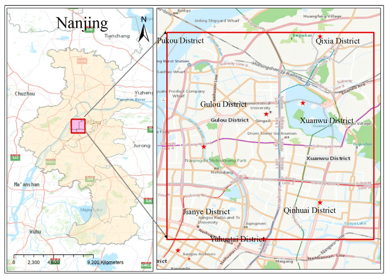
Figure 1Model domain of the PALM simulation used in the study for the city of Nanjing. The size of the model domain is approximately 10 km × 10 km. Map credit: ESRI 2020.
The model domain covers the core area of Nanjing with the center located at 32.07∘ N and 118.72∘ E (Fig. 1). The model horizontal resolution is 0.0001∘ × 0.0001∘ (equivalent to 9.4 m west–east × 11.1 m north–south) with a grid size of 960 × 960, which covers a total area of about 10 km × 10 km. To represent the CO air quality at pedestrian level, the model vertical layer depth starts from 2 m from the ground to 12 m height and stretched by a factor of 1.1 by each layer to a maximum of 40 m depth. The model has a total of 48 vertical layers reaching ∼ 1000 m a.s.l., which is approximately 3 times higher than the highest building of Nanjing (Zifeng Tower, 340 m height for the top floor). Further increasing the model domain height (e.g., to 2000 m) has no significant impact on the modeled airflow and CO concentrations near the ground as most of the buildings are lower than 150 m (Fig. 2a). The model is run for 3 h with a time step of 6 s. Hourly average data are achieved, and we use the results of the last hour for analysis.
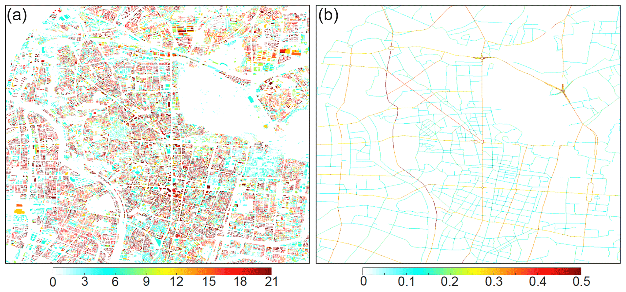
Figure 2Spatial distribution of (a) building heights (m) and (b) traffic CO emissions (mg cell−1 s−1) (during rush hours) in the model domain.
The topography of the model consists of two parts: baseline elevation and building heights. The former is based on the ASTER global digital elevation model (GDEM) dataset, which has a native resolution of 30 m and is linearly interpolated to the model grid (NASA, 2021). The building data for Nanjing are extracted from the Gaode Map (dated as the year 2018, https://ditu.amap.com, last access: 1 August 2020). The building data include the geographical location of the outer shape of buildings (0.0001∘ × 0.0001∘ resolution) and their number of floors. We transfer the raw data into the model grid and assume an average floor height of 3 m (Fig. 2a). The sum of the elevation and building height data are then used as the topographical data of the PALM. Due to the large computational cost associated with model simulation, we do not run the model for a consecutive time window with actual meteorological conditions. Instead, we choose a selective combination of meteorological scenarios to represent the variability of meteorological conditions at Nanjing. For each scenario, we assume a constant geostrophic wind field on the top of the boundary layer during model simulation. Eight wind directions with 45∘ between them (N, NE, E, SE, S, SW, W, and NW) are considered. Based on the observed wind speed at the top of the local boundary layer (∼ 500 m) (Chen et al., 2018; He et al., 2018), we choose 10, 6.5, and 3 m s−1 to represent high, median, and weak wind conditions, respectively. This results in a total of 48 scenarios, which is limited by our computational capacity. We thus consider our study as a demonstration of the model approach, and it can be improved by more scenarios.
2.2 Traffic emissions
We use a “standard road length” approach to assign the total traffic emissions to individual roads based on different road types and traffic flows (Zheng et al., 2009). We first transfer the actual road length (L) into total standard road length (TSL, km) of Nanjing using the road conversion coefficient (W):
where i, j, and k represent the area types (i.e., urban and suburban areas), grid cell index, and road type, respectively, with m, n, and o representing the total numbers of area types, grid cells, and road types, respectively. The W is calculated as follows:
where TF is the traffic flow for the kth road type and ith area type in grid j (in standard vehicles), and STF is the standard traffic flow (in standard vehicles).
The traffic emission (GEj) of each grid cell j is calculated based on the total standard road length in the grid cell (GSLj) and the standard emission intensity per standard unit length (SEI, t km−1).
where SEI is calculated based on the TSL calculated in Eq. (1) and the city-level-based vehicle emission inventories (E, t):
GSLj is calculated as
We also assign the daily mean GEj to each hour based on the diurnal variation of the 24 h traffic flow (Fig. 2b). The diurnal variation of the traffic flows and subsequently the traffic emissions at Nanjing are based on the Gaode Map (https://report.amap.com/detail.do?city=320100, last access: last access: 15 October 2020). The total traffic CO emissions in the model domain are 0.77 and 0.60 kg s−1 for rush and non-rush hours, respectively.
2.3 Taxi sensor data
We evaluate the model results with observations collected from a mobile platform that is performed during September 2019–October 2020. The details of the platform instrument and its deployment are described in Wang et al. (2020). Briefly, we use two XHAQSN-508 instruments (dimensions: 290 × 81 × 55 mm; weight: 1.0 kg) produced by Hebei Sailhero Environmental Protection High-tech Co., Ltd. (Hebei, China), which include an internal CO gas sensor (detectable CO range: 0 to 50 mg m−3) and are installed on the top of two Nanjing taxis (∼ 1.5 m above ground). The sensor is capable of continuously measuring CO concentrations at a programmable frequency of once every 10 s. The inlet system is also optimized to minimize self-sampling and gas sampling losses. The spatial coordinates are also recorded by a GPS device included in this instrument (u-blox, Switzerland). The monitoring and location data are simultaneously transmitted to a remote server in real time through wireless communication, and the real-time measurement data can be viewed through a web page or an Android app. One major advantage of this mobile platform is the minimum maintenance cost, as samples are automatically collected during the operation of the taxis. An analysis of the sensing power, defined as the fraction of city road network sampled by a taxi fleet, also demonstrates that a remarkably small number of taxis can scan a large number of streets (O'Keeffe et al., 2019; Wang et al., 2020).
The instrument is calibrated once per month against a stationary instrument (T300 CO Analyzer by Teledyne API) at the SORPES observation station in the Xianlin Campus of Nanjing University (https://as.nju.edu.cn/as_en/obsplatform/list.htm, last access: 1 November 2020). During calibration, the instrument is taken back to the campus and placed back-to-back to the calibrating instrument in the station. The calibration lasts for at least seven days, and the parameters for the sensor retrieval algorithm are adjusted to make sure the difference between the sensor-retrieved data and the station data is < 1 % (Wang et al., 2020). As only traffic-related emissions are considered in the PALM, we add the model results to the background concentrations of Nanjing for comparison to the observed data by the mobile platform (but the pure model output is used for other analyses). The hourly background CO concentrations are calculated as the minimum of measurements from all the nine national air quality monitoring stations in Nanjing metropolitan area (https://quotsoft.net/air/, last access: 24 February 2021). Seven of these stations are located inside the model domain representing different functioning districts of the city. The remaining two are located at the suburbs to the west and northeast of the city center, which could be a reasonable representative for background concentrations depending on wind directions. Corresponding hourly meteorological data of Nanjing city are obtained from the National Meteorological Information Center of China (http://data.cma.cn/en, last access: 1 November 2020). We include data on both rainy and non-rainy days as CO is not dissolvable.
3.1 Very high-resolution modeled CO concentration
Figure 3 shows an example of the spatial distribution of the modeled traffic-related ground-level (0–2 m above ground) CO concentrations during peak hours (with an east wind and 6.5 m s−1 at the top of boundary layer). The very high resolution of the model reveals a detailed geographical dispersion pattern of CO concentrations in and out of the road network. The average modeled CO concentrations inside the road network are 0.76 mg m−3 (with 25 % and 75 % percentiles as 0.45 and 0.94 mg m−3, respectively), which are much larger than those outside the network: 0.22 (0.14–0.24) mg m−3. The lowest concentrations are modeled over regions with a less dense road network and fewer water bodies (∼ 0.1 mg m−3). Higher ground-level concentrations are modeled over major highways with substantially higher emissions than other roads (Fig. 2b). The concentrations are also higher over interceptions of roads as the emissions are specified as the sum of those of the intercepted roads. The model simulates clear plumes downwind of major roads, especially if no obstacles existed in that direction. The most apparent plume is simulated in the northeast of the Xuanwu Lake (refer to the map in Fig. 3b). The high emissions are swept for about 1 km westward from a traffic center at the northeast edge of the lake. Highways such as the Neihuanxi line also produce apparent westward plumes, whereas downwind buildings may cause extra turbulence to smoothen out the signal. By contrast, the emissions from regions with dense buildings are generally trapped within the street canyons (e.g., the city center), with leakage from gaps between buildings (Fig. 3c). Overall, the modeled ground-level concentrations follow a two-mode Gaussian distribution (i.e., a sum of two Gaussian functions; Fig. 4), with one for residential streets (with a geometric mean of 0.17 mg m−3) and the other for arterial roads, highways, and the nearby regions (with a geometric mean of 0.28 mg m−3).
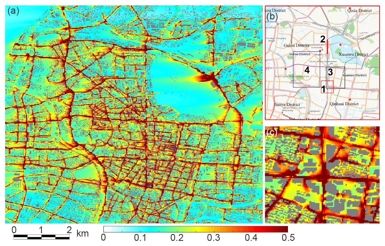
Figure 3Modeled ground-level CO concentrations (mg m−3) during rush hours by the PALM with wind from the east and speed as 6.5 m s−1 in the top of the boundary layer (a). Panel (b) shows the corresponding city map. Panel (c) shows a close-up of the Xinjiekou area with the boundary shown as a red rectangle in panel (b) (rectangle 1). Grey areas represent tops of buildings. Map credit: ESRI 2020.
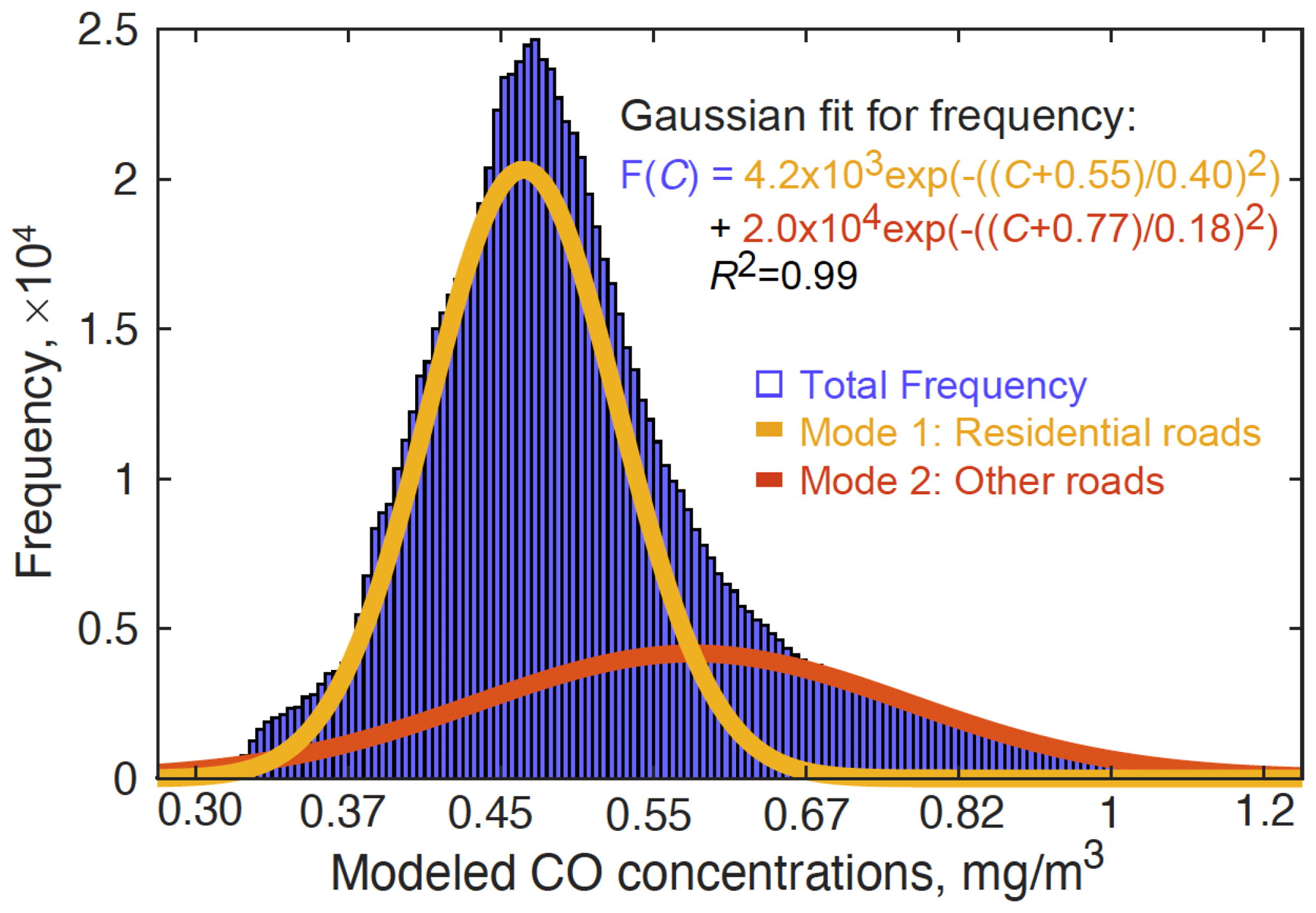
Figure 4Frequency distribution of modeled ground-level CO concentrations during rush hours under the east wind and 6.5 m s−1 at the top of boundary layer. The distribution is fitted with a two-mode Gaussian model. The yellow (residential streets) and orange (arterial roads, highways, and the nearby regions) curves represent the two Gaussian modes.
3.2 Model evaluation
The rich information provided by the model is compared to observations obtained by the mobile monitoring platform (Figs. 5 and 6). We sample the hourly-mean model results with the same location, emission level (rush or non-rush hours), and wind speed/directions as the observations. We aggregate the model results into a 100 m resolution due to the relatively low sampling frequency of the mobile sampler (10 s, equivalent to ∼ 100 m), which is indeed a drawback and can be improved by higher time-frequency sensors. The sum (0.92 ± 0.40 mg m−3) of model results that are caused by traffic-related sources (0.36 ± 0.32 mg m−3) and regional background concentrations (0.56 ± 0.28 mg m−3) agree well with the measured CO concentrations (0.90 ± 0.58 mg m−3, n=114 502) (p < 0.01). Point-by-point comparison reveals that most of the data points fall near the 1 : 1 line and are within lines for a factor-of-2 difference (Fig. 5). The model tends to overestimate the measured CO concentrations over the Neihuanxi Line (the line of points on the left of Fig. 5; location marked in Fig. 1), which is a viaduct with better ventilation than ground-level roads. However, our model considers all the emissions at the ground level and thus simulates much higher concentrations than observations over this line. This also demonstrates the significant air quality benefit of building a viaduct in an urban environment.
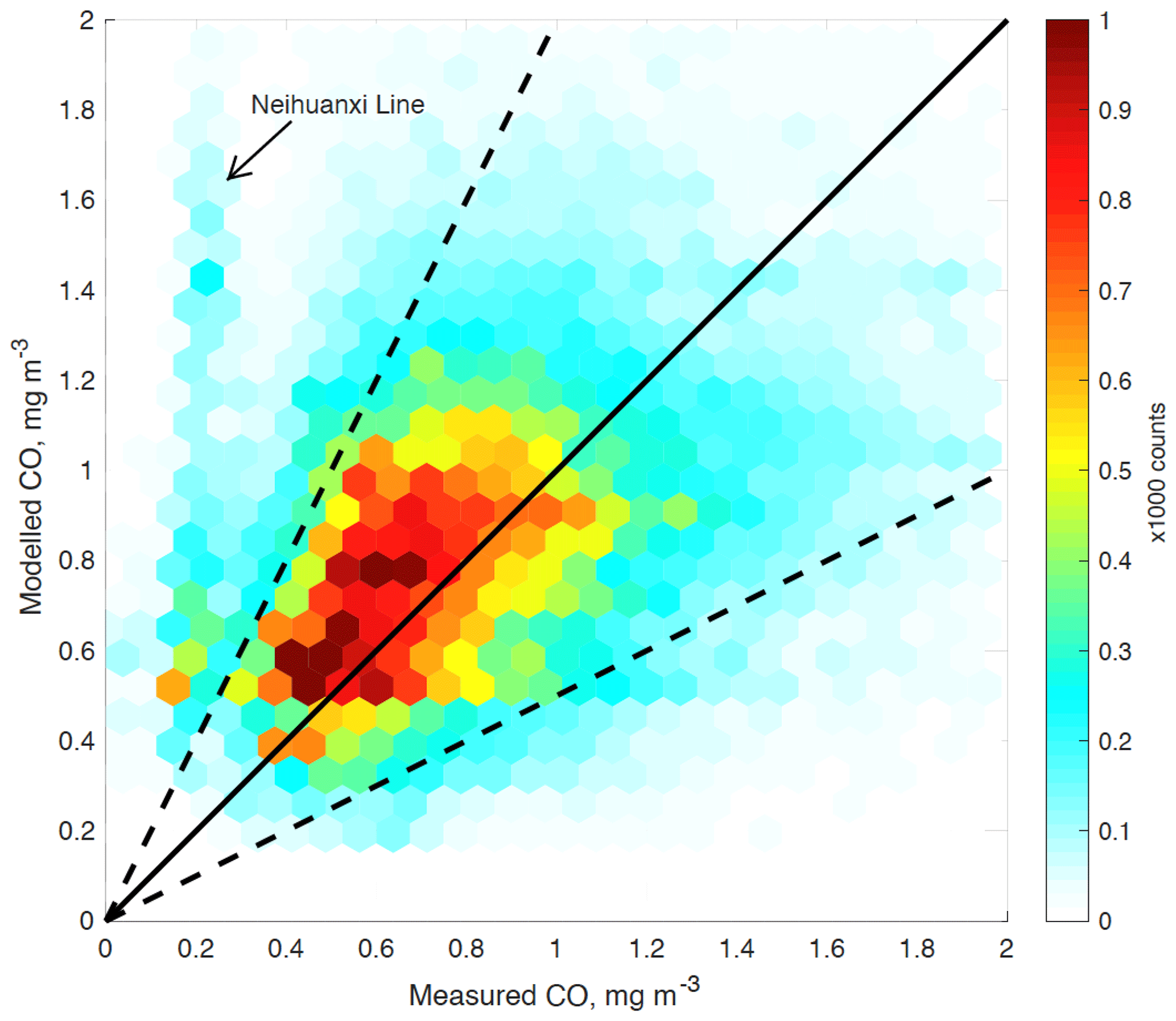
Figure 5Comparison of measured and modeled ground-level CO concentrations. Colors represent the total number of matching measured and modeled values contained within distinct hexagons. The black line indicates 1 : 1, and dashed lines mark a factor of 2 difference.
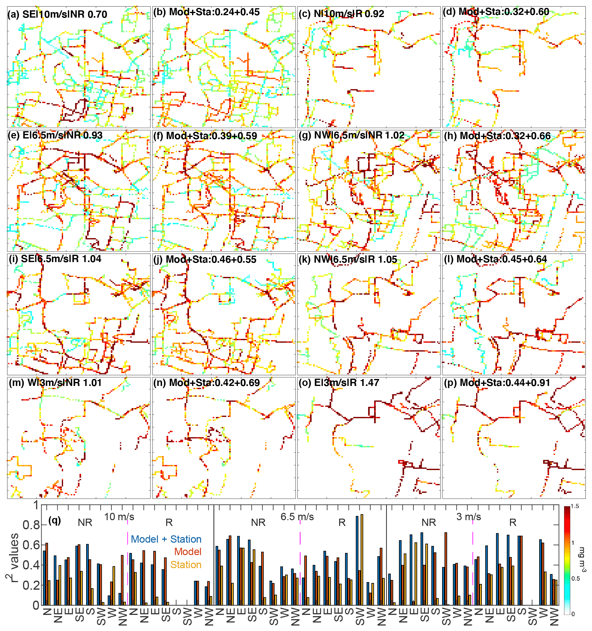
Figure 6Comparison between taxi-sensor-measured (odd columns) and modeled (even columns) ground-level CO concentrations for selected combinations of wind speed, directions, and rush/non-rush hours. As the taxi sensor data have a temporal resolution of 10 s (roughly equivalent to 100 m given an average vehicle speed of 40 km h−1), both the measurements and model results are regraded to a 100 m resolution grid. The wind and emission information is shown at the top of the panels in this format: “wind direction | wind speed | emission level rush or non-rush hours”. The mean of the data is shown at the top of each panel, with the modeled one as the sum of the model output and regional background from national stations. Panel (q) shows the coefficients of determination (r2) of a linear regression between taxi sensor data and model/station data under different emission and meteorological conditions. Blue bars represent the regression between measured and model + regional background, while red and yellow bars are for the measured vs. model only and measured vs. station data only, respectively. Note the color bar for panels (a)–(p) is in panel (q).
As both the modeled and measured CO concentrations vary drastically, we group the data based on the sampling time and meteorological conditions and compare the spatial patterns of model results and the measurements in Fig. 6. We find the model captures many of the observed spatial features under a variety of emission and meteorological conditions. Take 10 m s−1 east wind during non-rush hours as an example (Fig. 6a and b): higher concentrations are modeled and measured in the city center, the highway in north city, and the arterial roads in the southwest corner of the model domain, while lower concentrations are in the middle of the west part and southeast corner of the model domain. Similar levels of agreement between the spatial patterns of measurements and model results are achieved for other conditions.
Figure 6q shows that the coefficients of determination (r2) are generally higher (0.51 ± 0.16) during non-rush hours with middle and low wind speeds, due to the relatively larger sample sizes under such conditions. The r2 values for high wind conditions and rush hours will be increased as the accumulation of taxi sensor data (either longer sampling periods or more sensors). As the model data used in this comparison include the regional background, we calculate the r2 values if only using the station data to rule out the possibility that the agreement in spatial pattern is caused by station data. Also, taking the r2 values during non-rush hours with middle and low wind conditions as an example, only using station data lowers the r2 values to 0.28 ± 0.23. This indicates that our model indeed carries useful spatial information that significantly improves the comparison with sensor data.
One drawback of the taxi platform is that the popular streets are easily covered and sampled repeatedly, but unpopular segments are rarely visited (O'Keeffe et al., 2019; Wang et al., 2020). The sensor data used in this study mainly cover the highway and arterial roads but generally leave the model results for residential streets unevaluated. We therefore supplement the routine taxi operation data with two one-day taxi cruise campaigns, which cover all the public roads in two representative regions (especially including the residential ones less visited by taxis), as shown in Fig. 7 (the location of campaign is shown in Fig. 3b). Overall, the model captures the observed spatial patterns reasonably well with r2 values for the two campaigns of 0.50 and 0.37, comparable to the data collected during normal taxi operations (Fig. 6q). The first campaign is in the city center (Fig. 7a and b) with the traffic-related CO concentrations relatively more uniformly compared to the second one, which covers a larger area and includes highways, arterial, and residential roads (Fig. 7c and d). The model also captures the relatively higher concentrations in the highway near the west edge in the second campaign (Fig. 7c and d), as well as the generally decreasing concentrations from highways, arterial roads, to residential ones. Even though the model has highly simplified setups and the mobile sensors have relatively large uncertainties compared with reference method (Wang et al., 2020), the agreement between them lend both approaches confidence.
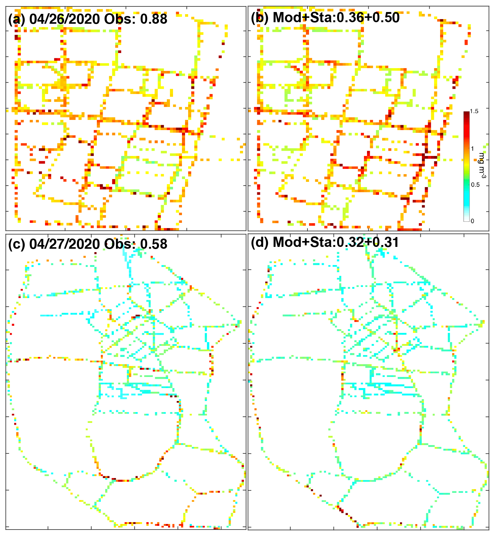
Figure 7Comparison between taxi-sensor-measured (a, c) and modeled (b, d) ground-level CO concentrations during two intensified observation campaigns during 26–27 April 2020. The locations of the campaigns are shown in Fig. 3b (rectangles 3 and 4 for the 26 and 27 April, respectively).
3.3 Influencing factors
3.3.1 Emissions, wind speed, and directions
Figure 8 shows the mean ground-level CO concentrations over the whole model domain under different emission strengths and meteorological factors. We find the wind speed is an important controlling factor for modeled CO concentrations. The average ground-level CO concentrations during rush hours with a wind speed of 3 m s−1 range from 0.37–0.46 mg m−3. The concentrations with 3 m s−1 wind are ∼ 2.4 and ∼ 1.8 times higher than those with 10 m s−1 (0.16–0.19 mg m−3) and 6.5 m s−1 (0.21–0.25 mg m−3) wind speeds, respectively. The concentration differences between 10 and 6.5 m s−1 are about 30 %. It clearly suggests a non-linear dependence of concentrations on wind speed with much higher concentrations over stagnant conditions, consistent with previous studies (Mumovic et al., 2006; Wolf et al., 2020). Indeed, convective transport of pollutants is greatly reduced under low wind speed conditions, which elevates CO concentrations at the pedestrian level. On the other hand, the response to emission strength is almost linear: the concentrations during rush hours are 27 % higher than non-rush hours given the same meteorological conditions. The concentrations with different wind directions vary by ∼ 20 %, with the highest concentration consistently shown for the west wind and the lowest for the northeast wind. This pattern could be explained by the spatial pattern of emission distributions: with higher emissions in the west part of the model domain and lower over the northeast (where a large lake is located). Wind from cleaner regions (e.g., northeast) helps to blow out the traffic-related emissions located at the other side of the model domain, and vice versa.
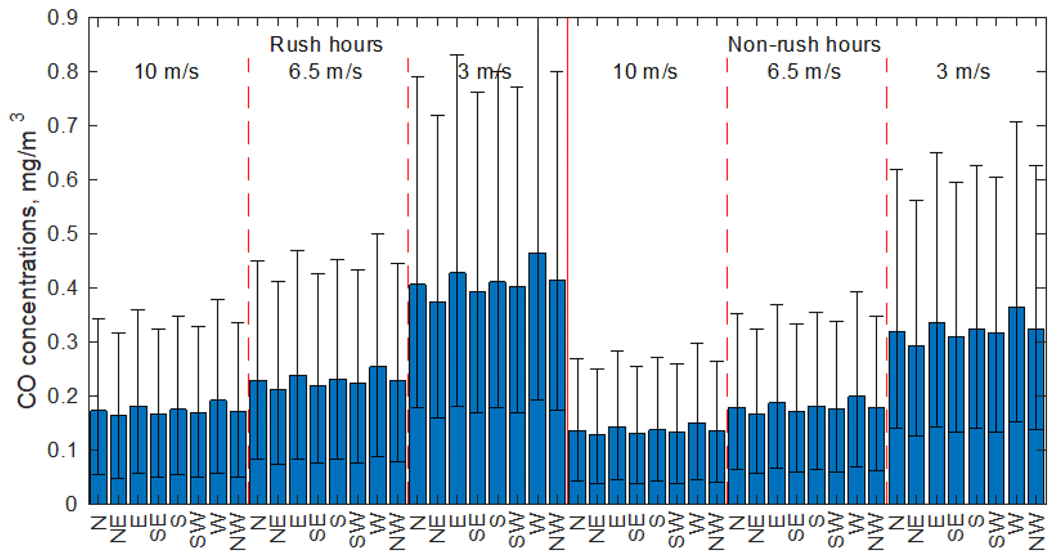
Figure 8Mean modeled ground-level CO concentrations (with 30 % and 70 % percentiles) over the whole model domain with different wind speeds, wind directions, and emission levels.
3.3.2 Street direction
Even though the wind direction seems not to be an important influencing factor for model domain-average concentrations, it is a vital factor for individual street canyons. Figure 9 shows the relationship between the mean ground-level CO concentrations and the angle between wind and street directions. We find the modeled concentrations are the highest when the wind direction aligns with streets. The concentrations decrease until the angle increases to ∼ 20∘, but no significant differences are modeled when the angles continue to increase. A wind direction parallel with the street mainly transports CO along the canyon, which traps pollutants inside of the street. By contrast, a perpendicular wind can blow pollutants outside of the canyon through gaps between buildings, which reduces the CO concentrations inside. Similar results have been found in smaller-scale studies. For example, through comparing pollutant levels with different wind directions, Kurppa et al. (2019) found lower pedestrian-level pollution when wind direction is closer to perpendicular with a boulevard and suggested building the shortest wall parallel to the road to increase ventilation and create optimal air quality. Solazzo et al. (2011) found both the highest observed and modeled NOx concentrations inside a street canyon under a “quasi-parallel” situation. Mumovic et al. (2006) also suggested an accumulation effect along those canyons whose axes are parallel to the wind direction.
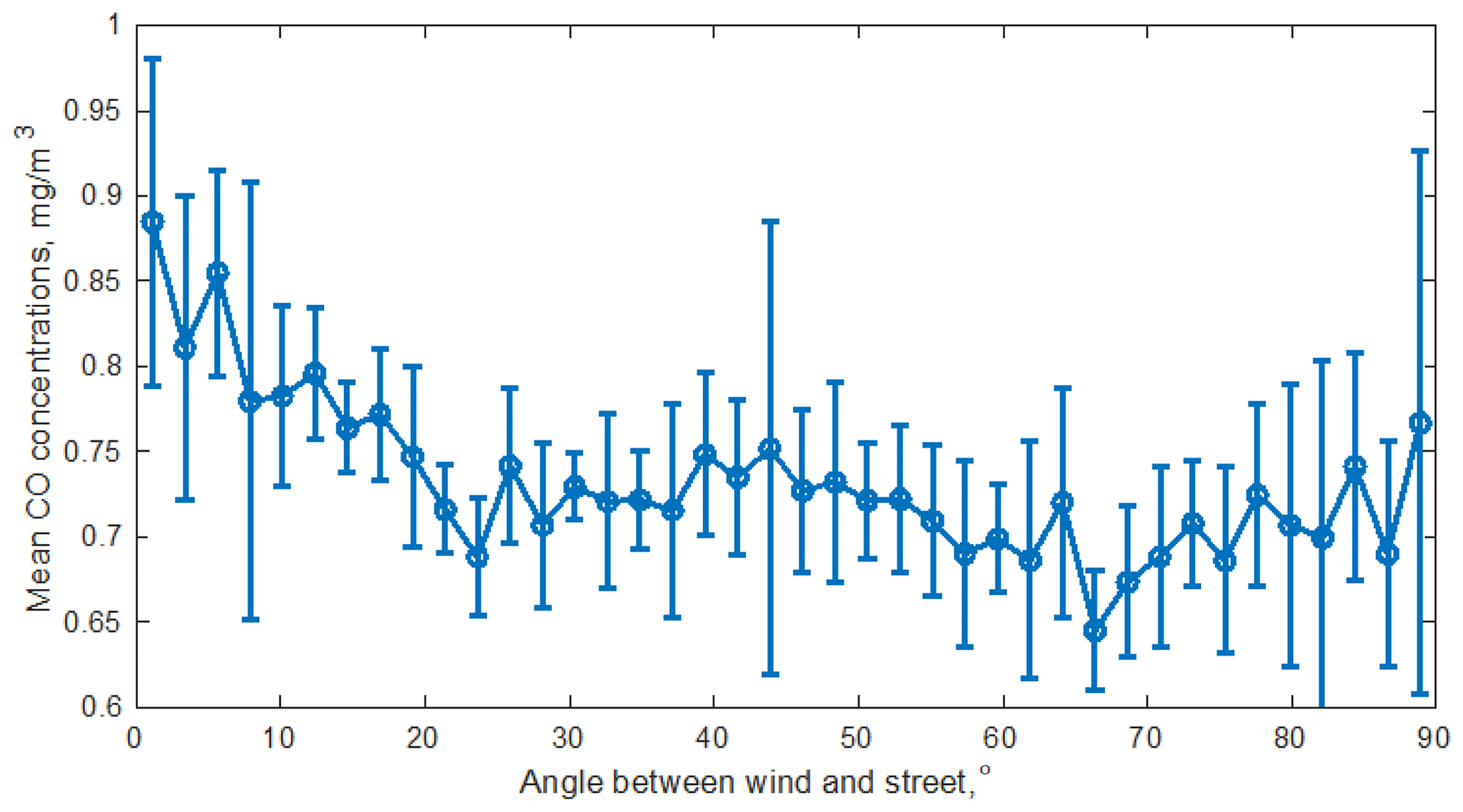
Figure 9Influence of the angle between the directions of the wind and the street on modeled ground-level CO concentrations. Wind speed is specified as 6.5 m s−1 with emissions as that during rush hours.
3.3.3 Building heights
The influence of street and wind directions on modeled CO concentrations is more obvious in a latitude–height cross section along a north–south direction street (Fig. 10). Figure 11 shows the CO concentrations in three longitude–height cross sections (marked as 1, 2, and 3 in Fig. 10a) to illustrate the leakage plumes from gaps between buildings. The modeled CO concentrations decrease sharply with height, as the sources are from near the ground (Fu et al., 2017). The buildings in the east side of this road that is close to the lake are lower than those in the west. The modeled CO concentrations are extended to a higher altitude behind the tall buildings under west wind conditions (Fig. 10a). The upwind buildings cause wake flows that transport pollutants toward the buildings at pedestrian level and make an accumulation zone at the leeward corners (Fig. 11a and d). By contrast, the traffic-related emissions are not elevated to a higher altitude with the east wind due to the short buildings on that side (Fig. 10b). Buildings located downwind of emission sources tend to create a flow pattern that blows pollutants away from them near the ground (Fig. 11b and c). Previous studies also found similar concentration gradients between leeward and windward of buildings when wind direction is perpendicular to the street canyon (Fu et al., 2017; Mumovic et al., 2006; Solazzo et al., 2011). For example, Fu et al. (2017) found that pollutants emitted inside the street canyon with lower leeward building heights than windward tend to disperse out of the canyon, and vice versa. When buildings exist on both sides of the street, the flow and concentration distributions are largely determined by which side the taller building is located on (Fig. 11e and f). The concentrations inside the street canyon are higher if the upwind building is taller than the downwind one.
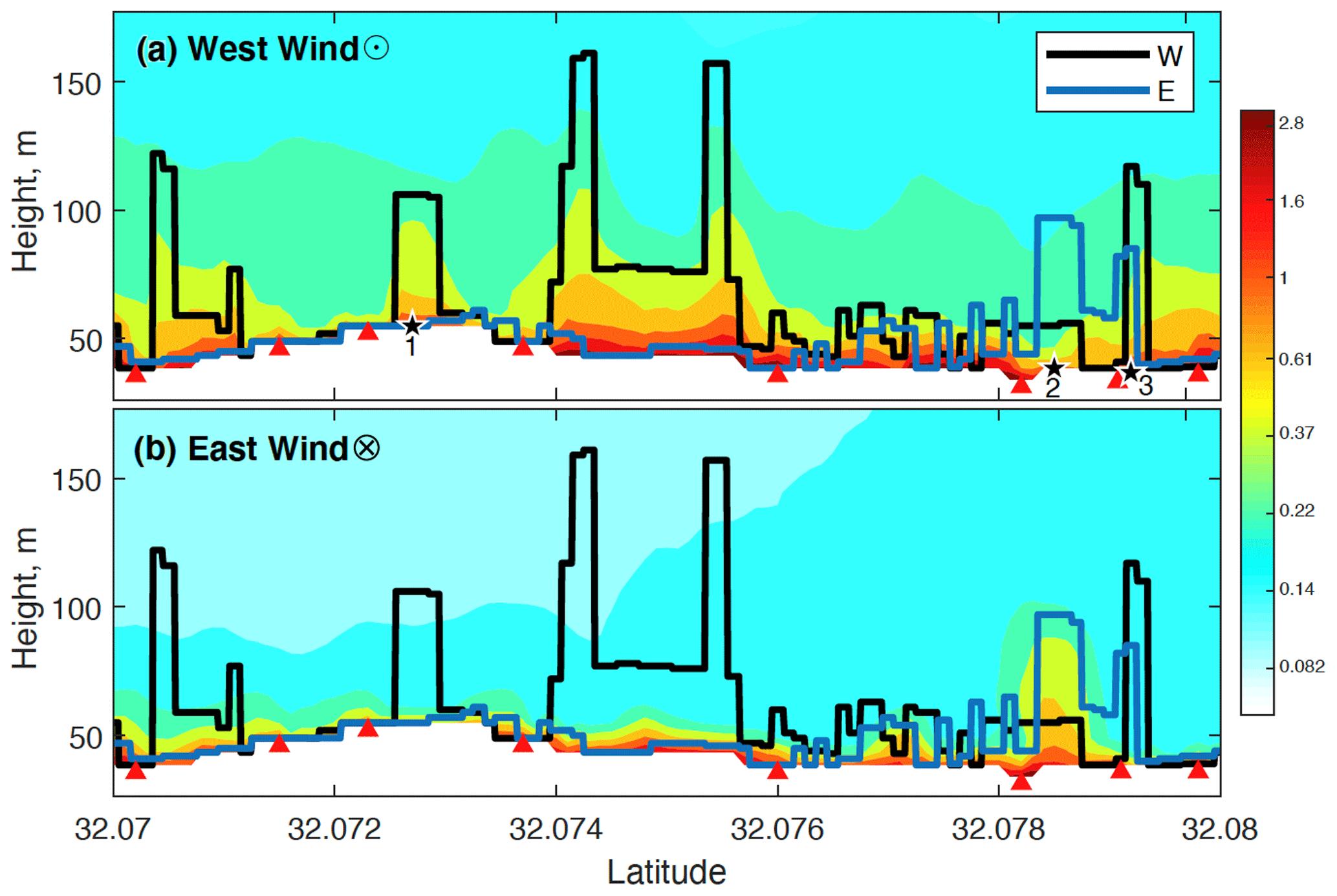
Figure 10Spatial distribution of modeled CO concentrations under west (a) and east (b) wind directions (3 m s−1) in latitude–height cross sections along Zhongyang Road during rush hours (marked as a red line 2 in Fig. 3b). The outlines of buildings on both sides of the road are shown as black (west side) and blue (east side) lines. Red triangles show the locations of major road intersections.

Figure 11Spatial distribution of modeled CO concentrations and wind vectors in longitude–height cross sections along three buildings on Zhongyang Road (marked as stars in Fig. 10a). The concentration distributions under west (a, c, e) and east (b, d, f) winds are shown. Note the vertical velocity is scaled by a factor of 2.5.
We also evaluate the relationship between the mean ground-level CO concentrations and the building heights in the upwind and downwind side of the street canyon in the whole model domain (Fig. 12). We find the existence of upwind buildings generally increases the CO concentrations inside the street canyon compared to cases without buildings in that direction (i.e., zero building height) (Fig. 12a). As discussed above, this is associated with the wake flow pattern of the building (Fig. 11a, d, and e). The concentrations show no significant difference when the upwind buildings are ∼ 10–45 m in height but decrease when building height further increases (Fig. 12a). The influence of downwind building heights are largely monotonically with lower concentrations for higher heights. The interaction of upwind and downwind building heights is evaluated by their differences (e.g., upwind – downwind heights). Overall, the concentrations are higher over street canyons with higher upwind buildings, but the enhancement in concentrations begins to decrease if the difference is larger than ∼ 30 m, consistent with Fig. 12a. Similarly, higher downwind buildings bring down the concentrations inside the canyon monotonically, consistent with Fig. 12b.
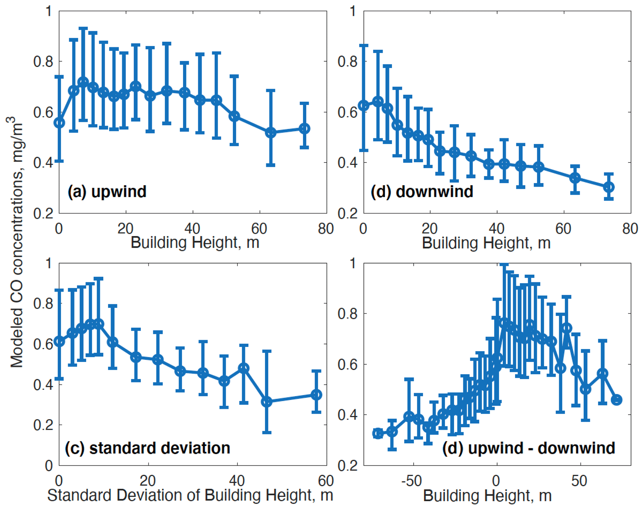
Figure 12Relationship between geometric mean modeled ground-level CO concentrations and building heights in the upwind (a) and downwind (b) directions, (c) the standard deviations of nearby (within 50 m distance) building heights, and (d) the difference between the upwind and downwind building heights. Wind speed is assumed to be 6.5 m s−1, and emissions are specified as that during rush hours.
Figure 12c illustrates the influence of the variation of building heights within 50 m distance on the modeled ground-level CO concentrations. It indicates that the concentrations first increase when the standard deviation of building heights increases from 0 to ∼ 10 m, reflecting the trapping effect of upwind buildings compared to flat surfaces. The concentrations significantly decrease when the nearby buildings are more variable. The variation in building heights has been demonstrated to increase the ventilation rates and the vertical turbulent flux density, which helps to lower pedestrian-level pollution (Kurppa et al., 2018). Fu et al. (2017) also found the concentration inside the street canyon first increased with the symmetric index of building heights but decreased when the index became larger. These results suggest putting higher buildings in the prevailing downwind side of a road with large variability in building heights and multiple gaps between them generates the best pedestrian-level air quality.
3.3.4 Distance to major roads
As discussed above, the modeled ground-level CO concentrations are higher inside the road network than outside of it. Figure 3 shows a clear decreasing trend of modeled concentrations from the road network to residential regions far away from the major roads. We thus calculate the distance from a given location to the nearest major roads (d), which include highways and arterial roads with emissions considered in this study (Fig. 2b). Figure 13 shows the mean modeled ground-level CO concentrations (C) and their standard deviations as a function of d. We used an exponential equation to fit this function: following Apte et al. (2017), where α represents the modeled background contribution from traffic-related sources, i.e., C(∞). β is the sensitivity of C to d, and k represents the spatial scale of the decay of C. The equation fits the modeled means well, despite the relatively large standard deviations especially when d is less than ∼ 50 m (Fig. 13). We find the α value decreases as wind speed increases, indicating lower background values with higher wind speed as discussed in the Sect. 3.3.1. Similarly, the β values also decrease with higher winds. However, we find nearly identical k values for all the wind speeds, suggesting that it is a universal parameter controlled by the atmospheric lifetime of pollutants but not influenced by meteorological conditions. Indeed, Apte et al. (2017) also found different k values for NO, BC, and NO2. Our k values are much smaller than those calculated by Apte et al. (2017) because they only consider the distance to the nearest highways, and their d values are much larger than ours. Our calculations are close to the model results of Biggart et al. (2020) in that NO2 concentrations also become quasi-stable ∼ 50 m away from a major highway.
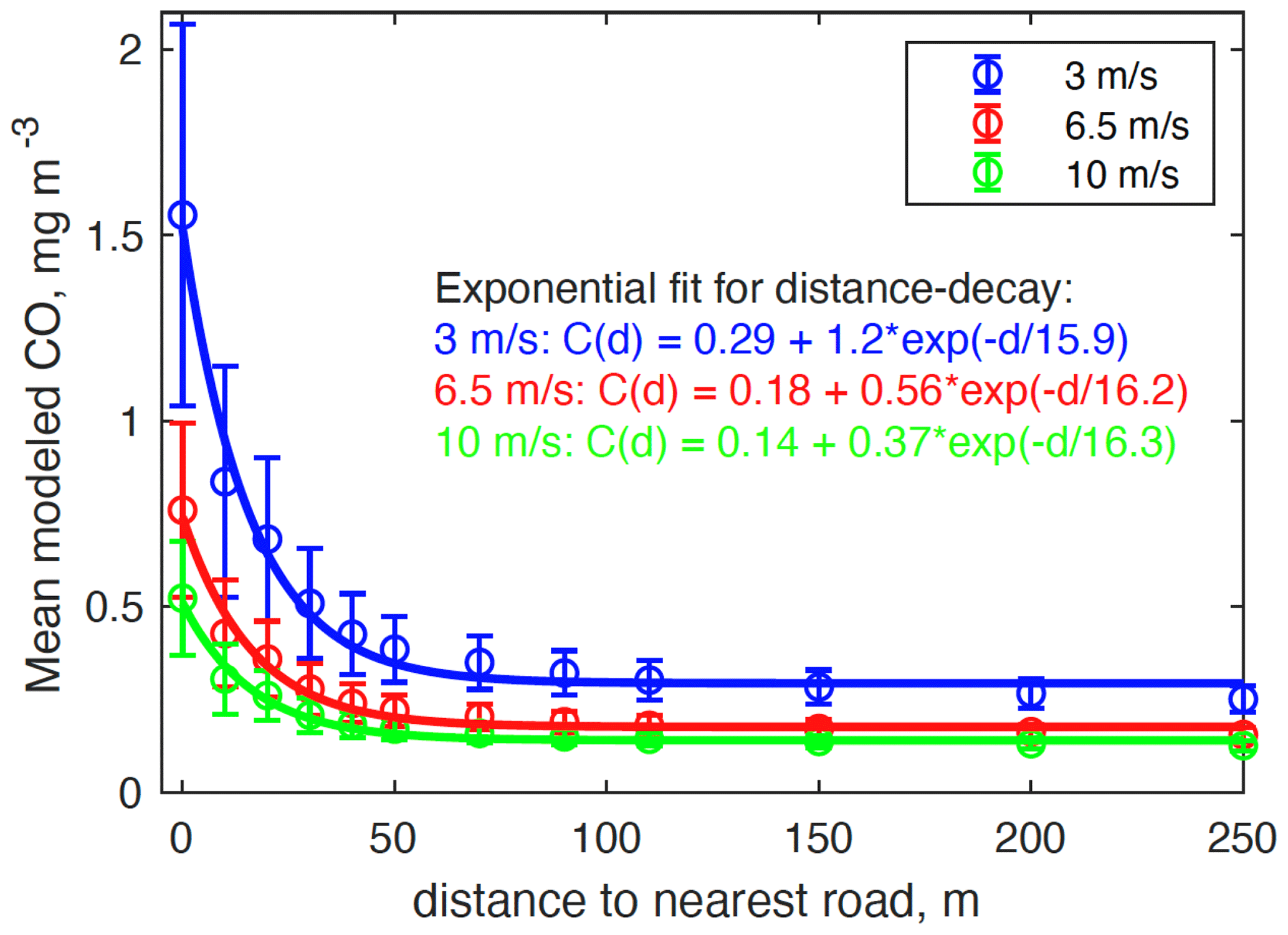
Figure 13Relationship between the modeled ground-level CO concentrations and the distance to the nearest major roads (assuming an east wind with emissions during rush hours). The circles and error bars are means and standard deviations, respectively.
This study demonstrates the potential of large-eddy simulation in urban air quality modeling. Future directions of the model include a more dynamic emission inventory that considers real-time vehicle speed and traffic congestion (Pan et al., 2016). The model frame is also readily expandable to include other pollutant sources (e.g., point and area sources), multiple pollutants, and their chemical reactions (Wolf et al., 2020; Zhong et al., 2015). More realistic meteorological conditions possibly nudging from larger-scale weather and climate data could replace the limited number of assumed scenarios as adopted in this study (Heinze et al., 2017).
The revealed high-resolution spatial variability and its association with underlying meteorological conditions are useful for developing parameterization schemes for statistical models like AERMOD and ADMS-Urban, and land use regression models (Jerrett et al., 2005). As high-resolution information on urban building and traffic distribution is becoming more available, the approach could be relatively easily applied to other cities. The simulated tremendously high-resolution maps of concentrations in all major urban areas will be a vigorous part of the smart city system (Silva et al., 2018) and serve as a data assimilation platform for many other products from satellite remote sensing and mobile platforms. The model results give hints for source contribution and hotspots for urban air pollution, which could inform urban planning, air quality management, and risk mitigation. Combined with personal GPS data, the very high resolution of air quality map revealed here can inform epidemiological studies and health risk analysis and alter personal behavior (Gao et al., 2019; Larkin and Hystad, 2017).
The model code and validation data used in this work are available at http://cn.ebmg.online/data/PALM/palm.zip (Zhang, 2021).
YZ and NZ designed the research. YZ, XY, SW, and ZW performed model simulations. YZ, LD, SW, YM, MY, YL, and QL analyzed data. XH and HW provided emission data. SW, LW, XC, AD, LZ, and YX provided validation data. YZ, SW, LD, and HW wrote the paper.
The authors declare that they have no conflict of interest.
This article is part of the special issue “Air Quality Research at Street-Level (ACP/GMD inter-journal SI)”. It is not associated with a conference.
We are grateful to the High Performance Computing Center (HPCC) of Nanjing University for doing the numerical calculations in this paper on its blade cluster system. We thank Rong Ye and Liang Luo for sample collection.
This research has been supported by the National Key R&D Program of China (grant no. 2019YFA0606803), National Natural Science Foundation of China (grant no. 71974092), Start-up fund of the Thousand Youth Talents Plan, Jiangsu Innovative and Entrepreneurial Talents Plan, and Collaborative Innovation Center of Climate Change of Jiangsu Province.
This paper was edited by Karine Sartelet and reviewed by two anonymous referees.
Abou-Senna, H., Radwan, E., Westerlund, K., and Cooper, C. D.: Using a traffic simulation model (VISSIM) with an emissions model (MOVES) to predict emissions from vehicles on a limited-access highway, J. Air Waste Manag. Assoc., 63, 819–831, https://doi.org/10.1080/10962247.2013.795918, 2013.
Apte, J. S., Messier, K. P., Gani, S., Brauer, M., Kirchstetter, T. W., Lunden, M. M., Marshall, J. D., Portier, C. J., Vermeulen, R. C. H., and Hamburg, S. P.: High-Resolution Air Pollution Mapping with Google Street View Cars: Exploiting Big Data, Environ. Sci. Technol., 51, 6999–7008, https://doi.org/10.1021/acs.est.7b00891, 2017.
Biggart, M., Stocker, J., Doherty, R. M., Wild, O., Hollaway, M., Carruthers, D., Li, J., Zhang, Q., Wu, R., Kotthaus, S., Grimmond, S., Squires, F. A., Lee, J., and Shi, Z.: Street-scale air quality modelling for Beijing during a winter 2016 measurement campaign, Atmos. Chem. Phys., 20, 2755–2780, https://doi.org/10.5194/acp-20-2755-2020, 2020.
Cécé, R., Bernard, D., Brioude, J., and Zahibo, N.: Microscale anthropogenic pollution modelling in a small tropical island during weak trade winds: Lagrangian particle dispersion simulations using real nested LES meteorological fields, Atmos. Environ., 139, 98–112, https://doi.org/10.1016/j.atmosenv.2016.05.028, 2016.
Chen, C., Meng, D., and Sun, P.: Research on Change Characteristics of wind speed at mid-low altitude layer over China based on radiosonde wind speed data, J. Arid Meteorol., 36, 82–89, 2018.
Fu, X., Liu, J., Ban-Weiss, G. A., Zhang, J., Huang, X., Ouyang, B., Popoola, O., and Tao, S.: Effects of canyon geometry on the distribution of traffic-related air pollution in a large urban area: Implications of a multi-canyon air pollution dispersion model, Atmos. Environ., 165, 111–121, https://doi.org/10.1016/j.atmosenv.2017.06.031, 2017.
Gao, Q. L., Li, Q. Q., Zhuang, Y., Yue, Y., Liu, Z. Z., Li, S. Q., and Sui, D.: Urban commuting dynamics in response to public transit upgrades: A big data approach, PLoS One, 14, 1–18, https://doi.org/10.1371/journal.pone.0223650, 2019.
He, J., Lu, C., Xie, S., Jiang, Y., and Han, Z.: Assessing the performance of wind profile radar in Nanjing and its application, J. Meteorol. Sci., 38, 406–415, 2018.
Heinze, R., Moseley, C., Böske, L. N., Muppa, S. K., Maurer, V., Raasch, S., and Stevens, B.: Evaluation of large-eddy simulations forced with mesoscale model output for a multi-week period during a measurement campaign, Atmos. Chem. Phys., 17, 7083–7109, https://doi.org/10.5194/acp-17-7083-2017, 2017.
Jaffe, L. S.: Ambient carbon monoxide and its fate in the atmosphere, J. Air Pollut. Control Assoc., 18, 534–540, https://doi.org/10.1080/00022470.1968.10469168, 1968.
Jeanjean, A. P. R., Hinchliffe, G., McMullan, W. A., Monks, P. S., and Leigh, R. J.: A CFD study on the effectiveness of trees to disperse road traffic emissions at a city scale, Atmos. Environ., 120, 1–14, https://doi.org/10.1016/j.atmosenv.2015.08.003, 2015.
Jerrett, M., Arain, A., Kanaroglou, P., Beckerman, B., Potoglou, D., Sahsuvaroglu, T., Morrison, J., and Giovis, C.: A review and evaluation of intraurban air pollution exposure models, J. Expo. Anal. Environ. Epidemiol., 15, 185–204, https://doi.org/10.1038/sj.jea.7500388, 2005.
Kumar, P., Morawska, L., Martani, C., Biskos, G., Neophytou, M., Di, S., Bell, M., Norford, L., and Britter, R.: The rise of low-cost sensing for managing air pollution in cities, Environ. Int., 75, 199–205, https://doi.org/10.1016/j.envint.2014.11.019, 2015.
Kurppa, M., Hellsten, A., Auvinen, M., Raasch, S., Vesala, T., and Järvi, L.: Ventilation and air quality in city blocks using large-eddy simulation-urban planning perspective, Atmosphere, 9, 1–27, https://doi.org/10.3390/atmos9020065, 2018.
Kurppa, M., Karttunen, S., Hellsten, A., and Järvi, L.: High-resolution urban air quality modelling using PALM 6.0, EMS (European meteorological society) Annual Meeting Abstracts, 9–13 September 2019, Copenhagen, Denmark, vol. 16, EMS2019-541, 2019.
Larkin, A. and Hystad, P.: Towards Personal Exposures: How Technology Is Changing Air Pollution and Health Research, Curr. Envir. Health Rpt., 4, 463–471, https://doi.org/10.1007/s40572-017-0163-y, 2017.
Letzel, M. O., Krane, M., and Raasch, S.: High resolution urban large-eddy simulation studies from street canyon to neighbourhood scale, Atmos. Environ., 42, 8770–8784, https://doi.org/10.1016/j.atmosenv.2008.08.001, 2008.
Li, C.: Features of the atmospheric stability at Nanjing area, in: Proceedings of the 9th forum of meteorological sciences at Yangtge River Delta, 24 November 2012, Zhenjiang, Jiangsu, China, 410–416, 2012.
Liu, H. and He, K.: Traffic optimization: A new way for air pollution control in China's urban areas, Environ. Sci. Technol., 46, 5660–5661, https://doi.org/10.1021/es301778b, 2012.
Mumovic, D., Crowther, J. M., and Stevanovic, Z.: Integrated air quality modelling for a designated air quality management area in Glasgow, Build. Environ., 41, 1703–1712, https://doi.org/10.1016/j.buildenv.2005.07.006, 2006.
NASA: ASTER Global Digital Elevation Map, available at: https://asterweb.jpl.nasa.gov/gdem.asp, last access date: 24 February 2021.
O'Keeffe, K. P., Anjomshoaa, A., Strogatz, S. H., Santi, P., and Ratti, C.: Quantifying the sensing power of vehicle fleets, Proc. Natl. Acad. Sci. USA, 116, 12752–12757, https://doi.org/10.1073/pnas.1821667116, 2019.
Pan, L., Yao, E., and Yang, Y.: Impact analysis of traffic-related air pollution based on real-time traffic and basic meteorological information, J. Environ. Manage., 183, 510–520, https://doi.org/10.1016/j.jenvman.2016.09.010, 2016.
Righi, S., Lucialli, P., and Pollini, E.: Statistical and diagnostic evaluation of the ADMS-Urban model compared with an urban air quality monitoring network, Atmos. Environ., 43, 3850–3857, https://doi.org/10.1016/j.atmosenv.2009.05.016, 2009.
Rood, A. S.: Performance evaluation of AERMOD, CALPUFF, and legacy air dispersion models using the Winter Validation Tracer Study dataset, Atmos. Environ., 89, 707–720, https://doi.org/10.1016/j.atmosenv.2014.02.054, 2014.
Sanchez, B., Santiago, J.-L., Martilli, A., Palacios, M., and Kirchner, F.: CFD modeling of reactive pollutant dispersion in simplified urban configurations with different chemical mechanisms, Atmos. Chem. Phys., 16, 12143–12157, https://doi.org/10.5194/acp-16-12143-2016, 2016.
Silva, B. N., Khan, M., and Han, K.: Towards sustainable smart cities: A review of trends, architectures, components, and open challenges in smart cities, Sustain. Cities Soc., 38, 697–713, https://doi.org/10.1016/j.scs.2018.01.053, 2018.
Solazzo, E., Vardoulakis, S., and Cai, X.: A novel methodology for interpreting air quality measurements from urban streets using CFD modelling, Atmos. Environ., 45, 5230–5239, https://doi.org/10.1016/j.atmosenv.2011.05.022, 2011.
Steffens, J. T., Heist, D. K., Perry, S. G., Isakov, V., Baldauf, R. W., and Zhang, K. M.: Effects of roadway configurations on near-road air quality and the implications on roadway designs, Atmos. Environ., 94, 74–85, https://doi.org/10.1016/j.atmosenv.2014.05.015, 2014.
Sun, J., Lenschow, D. H., LeMone, M. A., and Mahrt, L.: The Role of Large-Coherent-Eddy Transport in the Atmospheric Surface Layer Based on CASES-99 Observations, Boundary-Layer Meteorol., blackboxPlease provide volume number and page range or article number., https://doi.org/10.1007/s10546-016-0134-0, 2016.
The PALM Group: The PALM model system, available at: https://palm.muk.uni-hannover.de/trac, last access: 16 November 2020.
The World Bank: Urban population, available at: https://data.worldbank.org/indicator/SP.URB.TOTL.IN.ZS, last access: 16 November 2020.
US EPA: Air Quality Dispersion Modeling – Preferred and Recommended Models, available at: https://www.epa.gov/scram/air-quality-dispersion-modeling-preferred-and-recommended-models, last access: 16 November 2020.
van Donkelaar, A., Martin, R. V., Brauer, M., Kahn, R., Levy, R., Verduzco, C., and Villeneuve, P. J.: Global estimates of ambient fine particulate matter concentrations from satellite-based aerosol optical depth: Development and application, Environ. Health Perspect., 118, 847–855, https://doi.org/10.1289/ehp.0901623, 2010.
Vos, P. E. J., Maiheu, B., Vankerkom, J., and Janssen, S.: Improving local air quality in cities: To tree or not to tree?, Environ. Pollut., 183, 113–122, https://doi.org/10.1016/j.envpol.2012.10.021, 2013.
Wang, S., Ma, Y., Wang, Z., Wang, L., Chi, X., Ding, A., Yao, M., Li, Y., Li, Q., Wu, M., Zhang, L., Xiao, Y., and Zhang, Y.: Mobile monitoring of urban air quality at high spatial resolution by low-cost sensors: Impacts of COVID-19 pandemic lockdown, Atmos. Chem. Phys. Discuss. [preprint], https://doi.org/10.5194/acp-2020-1169, in review, 2020.
WHO: WHO Global Urban Ambient Air Pollution Database, available at: https://www.who.int/phe/health_topics/outdoorair/databases/cities/en/, (last access: 16 November 2020), 2016.
Wicker, L. J. and Skamarock, W. C.: Time-splitting methods for elastic models using forward time schemes, Mon. Weather Rev., 130, 2088–2097, https://doi.org/10.1175/1520-0493(2002)130<2088:TSMFEM>2.0.CO;2, 2002.
Wolf, T. and Esau, I.: A proxy for air quality hazards under present and future climate conditions in Bergen, Norway, Urban Clim., 10, 801–814, https://doi.org/10.1016/j.uclim.2014.10.006, 2014.
Wolf, T., Pettersson, L. H., and Esau, I.: A very high-resolution assessment and modelling of urban air quality, Atmos. Chem. Phys., 20, 625–647, https://doi.org/10.5194/acp-20-625-2020, 2020.
Yu, H. and Thé, J.: Simulation of gaseous pollutant dispersion around an isolated building using the k-Ω SST (shear stress transport) turbulence model, J. Air Waste Manag. Assoc., 67, 517–536, https://doi.org/10.1080/10962247.2016.1232667, 2017.
Zhang, Y.: Model code and data for this work, EBMG, available at: http://cn.ebmg.online/data/PALM/palm.zip, last access: 24 February 2021.
Zhang, Y., Tao, S., Shen, H., Jianmin, M., and Ma, J.: Inhalation exposure to ambient polycyclic aromatic hydrocarbons and lung cancer risk of Chinese population, Proc. Natl. Acad. Sci. USA, 106, 21063–21067, https://doi.org/10.1073/pnas.0905756106, 2009.
Zheng, J., Che, W., Wang, X., Louie, P., and Zhong, L.: Road-network-based spatial allocation of on-road mobile source emissions in the pearl river delta region, China, and comparisons with population-based approach, J. Air Waste Manag. Assoc., 59, 1405–1416, https://doi.org/10.3155/1047-3289.59.12.1405, 2009.
Zhong, J., Cai, X. M., and Bloss, W. J.: Modelling the dispersion and transport of reactive pollutants in a deep urban street canyon: Using large-eddy simulation, Environ. Pollut., 200, 42–52, https://doi.org/10.1016/j.envpol.2015.02.009, 2015.