the Creative Commons Attribution 4.0 License.
the Creative Commons Attribution 4.0 License.
 | 11 May 2021
Mobile monitoring of urban air quality at high spatial resolution by low-cost sensors: impacts of COVID-19 pandemic lockdown
Shibao Wang
Yun Ma
Zhongrui Wang
Lei Wang
Xuguang Chi
Aijun Ding
Mingzhi Yao
Yunpeng Li
Qilin Li
Mengxian Wu
Ling Zhang
Yongle Xiao
The development of low-cost sensors and novel calibration algorithms provides new hints to complement conventional ground-based observation sites to evaluate the spatial and temporal distribution of pollutants on hyperlocal scales (tens of meters). Here we use sensors deployed on a taxi fleet to explore the air quality in the road network of Nanjing over the course of a year (October 2019–September 2020). Based on GIS technology, we develop a grid analysis method to obtain 50 m resolution maps of major air pollutants (CO, NO2, and O3). Through hotspot identification analysis, we find three main sources of air pollutants including traffic, industrial emissions, and cooking fumes. We find that CO and NO2 concentrations show a pattern: highways > arterial roads > secondary roads > branch roads > residential streets, reflecting traffic volume. The O3 concentrations in these five road types are in opposite order due to the titration effect of NOx. Combined the mobile measurements and the stationary station data, we diagnose that the contribution of traffic-related emissions to CO and NO2 are 42.6 % and 26.3 %, respectively. Compared to the pre-COVID period, the concentrations of CO and NO2 during the COVID-lockdown period decreased for 44.9 % and 47.1 %, respectively, and the contribution of traffic-related emissions to them both decreased by more than 50 %. With the end of the COVID-lockdown period, traffic emissions and air pollutant concentrations rebounded substantially, indicating that traffic emissions have a crucial impact on the variation of air pollutant levels in urban regions. This research demonstrates the sensing power of mobile monitoring for urban air pollution, which provides detailed information for source attribution, accurate traceability, and potential mitigation strategies at the urban micro-scale.
- Article
(15010 KB) - Full-text XML
- Companion paper
-
Supplement
(4304 KB) - BibTeX
- EndNote


Urban air pollution poses a serious health threat with > 80 % of the world's urban residents exposed to air pollution levels that exceed the World Health Organization (WHO) guidelines (WHO, 2016). The global urban air pollution (measured by PM10 or PM2.5) also increased by 8 % during recent years despite improvement in some regions (WHO, 2018). Extremely large spatial variability exists for urban air pollutants (e.g., carbon monoxide, CO; nitrogen dioxide, NO2; and ozone, O3) over scales from kilometers to meters, as a result of complex flow patterns, non-linear chemical reactions, and unevenly distributed emissions from vehicle and industrial activities (Apte et al., 2017; Miller et al., 2020). Here we illustrate an approach to obtain a high-resolution urban air quality map using low-cost sensors deployed on a routinely operating taxi fleet.
High spatiotemporal resolution air quality data are critical to urban air quality management, exposure assessment, epidemiology study, and environmental equity (Apte et al., 2011, 2017; Boogaard et al., 2010). Numerous methodologies have been developed to obtain urban air pollutant concentrations, including stationary monitoring networks (Cavellin et al., 2016), near-roadway sampling (Karner et al., 2010; Zhu et al., 2009; Padro-Martinez et al., 2012), satellite remote sensing (Laughner et al., 2018; Xu et al., 2019), land use regression (LUR) models (Weissert et al., 2020), and chemical transport models (CTMs) (Li et al., 2010). However, the stationary monitoring stations (including near-roadway sampling) are sparsely and unevenly distributed, and the ability to reflect the details of urban air pollution is limited, especially at remote communities (Snyder et al., 2013). Remote sensing and CTMs are generally spatially coarse (∼ km resolution) and cannot resolve species that are inert to radiative transfer (e.g., mercury and lead) or without known emission inventory and/or chemical mechanisms. A LUR model can estimate concentrations at high spatial resolution, but it provides limited temporal information, and the predicting power is poor in areas with specific local sources (Kerckhoffs et al., 2016).
Mobile monitoring is a promising approach to garner high-spatial-resolution observations representative of the community scale (Miller et al., 2020; Hasenfratz et al., 2015). Different vehicle platforms are used for mobile monitoring, including minivans (Isakov et al., 2007), bicycles (Bart et al., 2012), taxi (O'Keeffe et al., 2019), Street View cars (Apte et al., 2017), and city busses (Kaivonen and Ngai, 2020). However, the scale of deployment and subsequent data coverage are limited by the cost of the observation instrument (Bossche et al., 2015). This issue has been addressed by the development of low-cost sensors that are calibrated with machine-learning-based algorithms (Miskell et al., 2018; SM et al., 2019; Lim et al., 2019). The emergence of low-cost air monitoring technologies was recognized by the US EPA (Snyder et al., 2013) and European Commission (Kaur et al., 2007) and was also recommended to be incorporated in the next Air Quality Directive (Borrego et al., 2015). For example, Weissert et al. (2020) combined land use information with low-cost sensors to obtain hourly O3 and NO2 concentration distribution at a resolution of 50 m. High agreements were also found between well-calibrated low-cost sensor systems and standard instrumentations (Chatzidiakou et al., 2019; Hagan et al., 2019).
The objective of this study is to illustrate the sensing power of low-cost sensors deployed on a routinely operating taxi fleet platform in a megacity. We combine mobile observations and a geographic information system (GIS) to obtain the hourly distribution of multiple air pollutant concentrations at 50 m resolution. By comparing these to the measurements from background sites, the contribution of traffic emission to urban air pollution is also diagnosed. We explore the influencing factors of pollutant levels including time of the day, day of the week, and holidays. Moreover, our sampling period covered the outbreak of COVID-19 in China. The pandemic lockdown had a tremendous impact on the socio-economic activities especially the traffic sector, and subsequently the air quality (Zhang et al., 2021; Huang et al., 2021). We evaluate how urban air quality changes in different periods of the pandemic and explore the impact of traffic-related emissions.
2.1 Mobile monitoring
We use the mobile sampler XHAQSN-508 from Hebei Sailhero Environmental Protection High-tech Co., Ltd. (Hebei, China) to measure the air quality in the Nanjing urban area. The instrument is equipped with internal gas sensors for CO (model XH-CO-50-7), NO2 (XH-NO2-5AOF-7), and O3 (XH-O3-1-7) (dimensions: 290 × 81 × 55 mm; weight: 1.0 kg) as well as two small in-built sensors for temperature and relative humidity and is fixed in the top lamp support pole (∼ 1.5 m above ground) of two Nanjing taxis (Fig. 1). Two taxis fueled with electricity and liquefied natural gas (one each) are selected to reduce the impact of emissions from the sampling vehicles themselves. All three sensors are electrochemical, which based on a chemical reaction between gases in the air and the electrode in a liquid inside a sensor that can detect gaseous pollutants at levels as low as parts per billion (Maag et al., 2018). Sensors are continuously powered by an external DC 12 V power supply provided by a taxi battery. The sample is refreshed by pumping air to the sensors. There is an air inlet at the bottom of the instrument, which is also checked periodically to avoid blockage. Because it is fixed in the taxi top lamp, it can reduce the impact of different wind direction airflow. This device integrates components for data integration, processing, and transmission and provides data management, quality control, and visualization functions. Pollutant concentration data are generated by different voltage values sensed by gas sensors, which are automatically uploaded to a database in the cloud via the 4G telecommunications network. We continuously measured the concentration of CO, NO2, and O3 in the street canyon in the urban area of Nanjing (with the center located at 32.07∘ N and 118.72∘ E) for a whole year (1 October 2019–30 September 2020). An instantaneous measurement of CO, NO2, and O3 concentrations is configured to continuous measurements at a frequency of once per 10 s sampling interval, and their limits of detection are 0.01 µmol mol−1, 0.1 nmol mol−1, and 0.1 nmol mol−1, respectively. The sampling routes were relatively random during taxi operations and were mainly on the arterial roads. A GPS device (u-blox, Switzerland) is utilized to record the spatial coordinates, and the spatial offsets are corrected by ArcGIS 10.2 software. Generally, the sampling campaign is conducted on both weekdays and weekends from 06:00 to 22:00 local time (LT). Occasionally the taxi drivers work for the night shift, and the instruments are run from 22:00 to 06:00 LT. The collected data cover 373 km2 with a population of 6 million (Fig. 1).
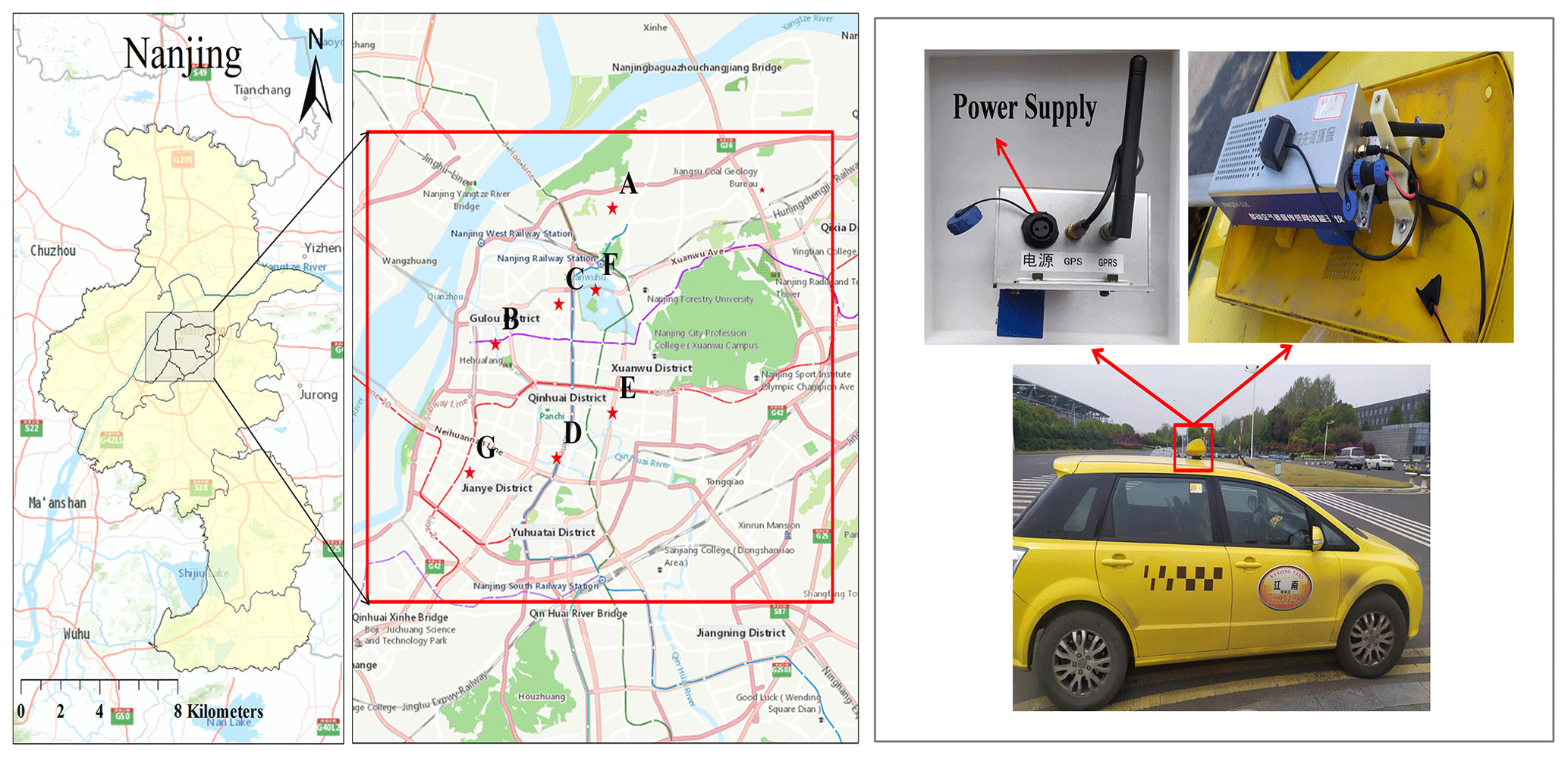
Figure 1Location of the monitoring areas in the city of Nanjing (left) and photo of instrument installment (right). Red stars are the locations of stationary stations belonging to the national air quality measurement network of China. These stations cover different functional regions of the city: A, B, C, D, E, F, and G represent industrial, cultural and educational, commercial, traffic, residential, ecological park, and new urban areas, respectively. Map credit: ESRI 2020.
2.2 Sensors calibration and validation
Different from traditional instruments, low-cost sensors have some limitations, such as nonlinear response, signal drift, environmental dependencies, low selectivity, and cross-sensitivity, so it is important that calibration procedures are applied with respect to these limitations (Maag et al., 2018; Lösch et al., 2008). For example, environmental conditions are known to cause nonlinear behavior of sensors (Popoola et al., 2016). Due to aging and impurity effects over a long time, low-cost sensors are prone to signal drift and low sensitivity (Kizel et al., 2018). In addition, cross-sensitivities differ largely according to the ambient temperature and level of gas the sensor is being exposed to (Lösch et al., 2008). So, multi-parameter joint calibration training is utilized to reduce the interference issue between air pollutants in our research, including air pollutant concentrations, temperature, and relative humidity. The sensors are usually trained with co-located data collected by reference methods before being deployed to actual measuring campaigns (Kaivonen and Ngai, 2020; Chatzidiakou et al., 2019; Bossche et al., 2015).
The XHAQSN-508 is calibrated every month starting from September 2019. The instrument is placed at the outdoor Station for Observing Regional Processes of the Earth System (SORPES) in the Xianlin Campus of Nanjing University (https://as.nju.edu.cn/as_en/obsplatform/list.htm, last access: 22 May 2021) for at least seven days before the taxi began sampling. The collected data are calibrated against standard instruments (Thermo Fisher Scientific 48i, 42i, and 49i, USA, for CO, NO2, and O3, respectively). The instrument precision is ±2 ppbv for O3 and ±1 % and ±4 % for CO and NO2, respectively, which have been used in many other studies and found to perform well for long-term runs (Ding et al., 2013; Herrmann et al., 2013). One drawback of our study is that the air pollutant concentrations observed at SORPES are lower than those observed in a road environment, which might cause issues for the calibration process. Comparing different calibration models, we found that a machine learning algorithm can improve sensor–monitor agreement with reference monitors, and many previous studies have used this method (Qin et al., 2020; Esposito et al., 2018; Vito et al., 2018). A supervised machine learning methodology based on the gradient boost decision tree (GBDT) is used for data calibration (Johnson et al., 2018). GBRT, an ensemble learning method, is a decision-tree-based regression model that implements boosting to improve model performance using both parameter selection and k-fold cross-validation. GBRT needs to be trained by the dataset with target labels (Yang et al., 2017). It takes input variables including raw signals of sensors, air pollutant concentrations (CO, NO2, and O3), temperature, and relative humidity. The stationary instrument data are taken as training targets. The parameters of the machine learning model are adjusted continuously based on a gradient descent algorithm. The R2 of the calibration results is generally high (> 0.90) for all the three air pollutants (e.g., Fig. 2a).
The success of supervised model training with target labels (i.e., co-located with SORPES, Fig. 2a) does not guarantee its predicting power for conditions without labels (i.e., on roads or co-located with SORPES but not feeding the station data to the algorithm; Fig. 2b). We use a calibration–validation methodology to evaluate the performance of the calibrated sensors (Chatzidiakou et al., 2019). This method includes two phases: first, the sampler was calibrated against the SORPES station for 10 d (1–10 June 2020), and the sensor data were used for sensor algorithm training as described above (Fig. 2a); second, we continued to place the sampler in the station (11–17 June 2020). However, the sensor data are not used for calibration but directly fed in the algorithm trained in the first phase. The results are compared with the station data (i.e., validation phase; Fig. 2b). We find that the sensor data agree well with standard instrumentation in the second phase. The sensor-retrieved CO, NO2, and O3 concentrations are 0.58 ± 0.12 mg m−3, 8.40 ± 4.30 µg m−3, 27.3 ± 16.5 µg m−3 respectively, not significantly different from those measured by standard instruments (0.50 ± 0.10 mg m−3, 10.5 ± 6.31 µg m−3, and 32.4 ± 20.2 µg m−3) (α=0.05, ANOVA analysis). The R2 values generally remain high (0.82–0.97) for different air pollutants (CO and O3) except for NO2 (R2=0.67). The lower R2 value for NO2 may be associated with the higher humidity during the validation period (13–16 June 2020). As NO2 is water dissolvable, high relative humidity may lead to a low bias for sensors (Wei et al., 2018). To improve performance of the NO2 model, temperature and relative humidity have also been involved in the training algorithm. However, the interaction between O3 and NO2 may influence the detection accuracy of these two chemicals, especially for NO2 (Ivanovskaya et al., 2001). The accuracy of the sensor generally decreases with time (a.k.a. aging) due to the evaporation of the electrolyte (Ribet et al., 2018). However, we find no significant decrease in the R2 values for the three pollutants during our campaign. It seems that the machine-learning algorithm could successfully compensate the aging of the sensors. Field calibration of low-cost sensors is still a challenging task, as it is greatly affected by atmospheric composition and meteorological conditions (Spinelle et al., 2017; Castell et al., 2017). Our results have high R2 values compared to previous studies, indicating relatively high accuracy (e.g., Castell et al., 2017). The results from the two sensors also agree with each other reasonably well, with R2 values ranging 0.97–0.99 for a linear regression. Their data are thus combined in the following analysis to achieve maximum data coverage. Overall, the sensor results have substantial uncertainty compared to reference methods. We thus focus on the relative temporal and spatial distributions rather than the absolute concentrations.
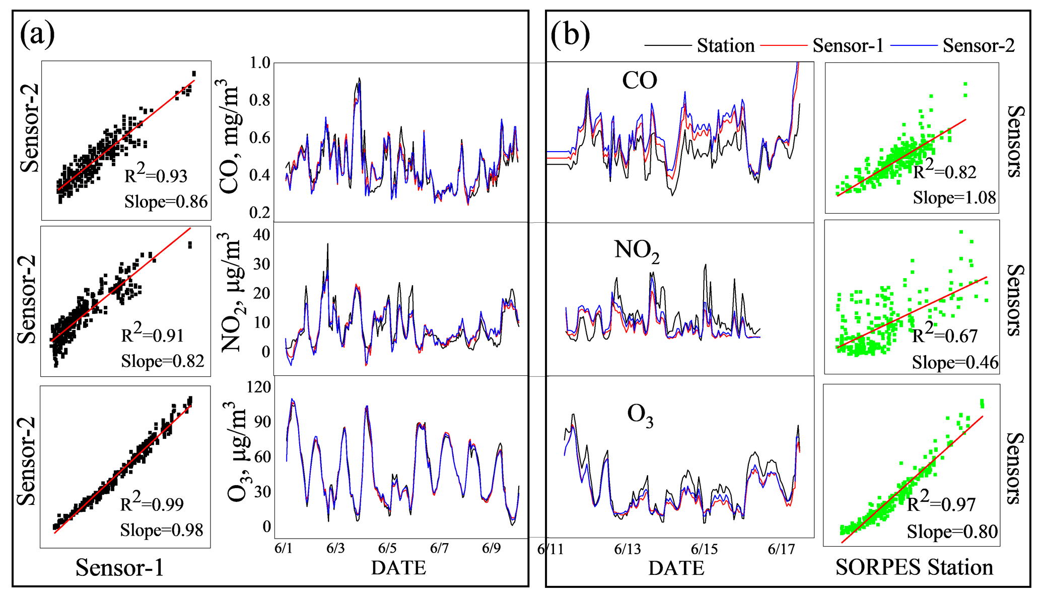
Figure 2Sensor performance evaluated by a calibration-validation methodology for CO, NO2, and O3. (a) Calibration period (1–10 June 2020); (b) validation period (11–17 June 2020). The time series plots compare the concentrations measured by the co-located sensors and standard instruments, while the scatterplots show pollutant concentrations and linear regressions between them.
2.3 Data processing
As the mobile monitoring platform samples along the trajectories of carrying vehicles, we need to sacrifice either the temporal information to calculate the spatial distribution of air pollutants, or the spatial information to temporal variations. Similar approaches have also been adopted by previous studies (Bossche et al., 2015; Apte et al., 2017; Farrell et al., 2015). To generate the spatial distribution of air pollutants at high spatial resolution, we divide the research area into grids with 50 m × 50 m resolution and calculate the mean values of the samples collected in each grid. The driving condition is highly variable and the taxi can travel more than 50 m in 10 s if the vehicle speed is over 18 km/h. However, given the complexity of the driving conditions, we ignore the vehicle trajectory in the past 10 s but assign the measured values to the location of the vehicle at the time of data uploading. Then, combined with GIS technology, we calculate the average of all the data points over one year that fall in the same grid. One drawback of our study is the impact of spike concentrations on sensor performance. The sensors keep reporting high concentrations in an approximate 1 min period after exposure to large environmental concentration spikes. This effect would reduce the effective resolution of our gridded concentration map. Similarly, we calculate the hourly average concentrations by considering only the data sampled in the same hour of different days. The GPS signal is missing when the taxis pass through the nine underground tunnels in Nanjing (e.g., Xuanwu lake tunnel and Jiuhuashan tunnel in the city center; Fig. 3). We assume the taxies travel at a constant speed and the sampling points are uniformly allocated along the tunnels. We use the ArcGIS 10.2 software for data processing. To calculate the air pollutant concentrations (CO, NO2, and O3) of different road types and the contribution of traffic emissions to them, we divide the urban roads in Nanjing area into six types, including highways, arterial roads, secondary roads, branch roads, residential streets, and tunnels (https://wiki.openstreetmap.org/wiki/Key:highway, last access: 21 January 2021). The roads and land use data of Nanjing shown in Fig. 3 are based on OpenStreetMap (OpenStreetMap contributors, 2020).
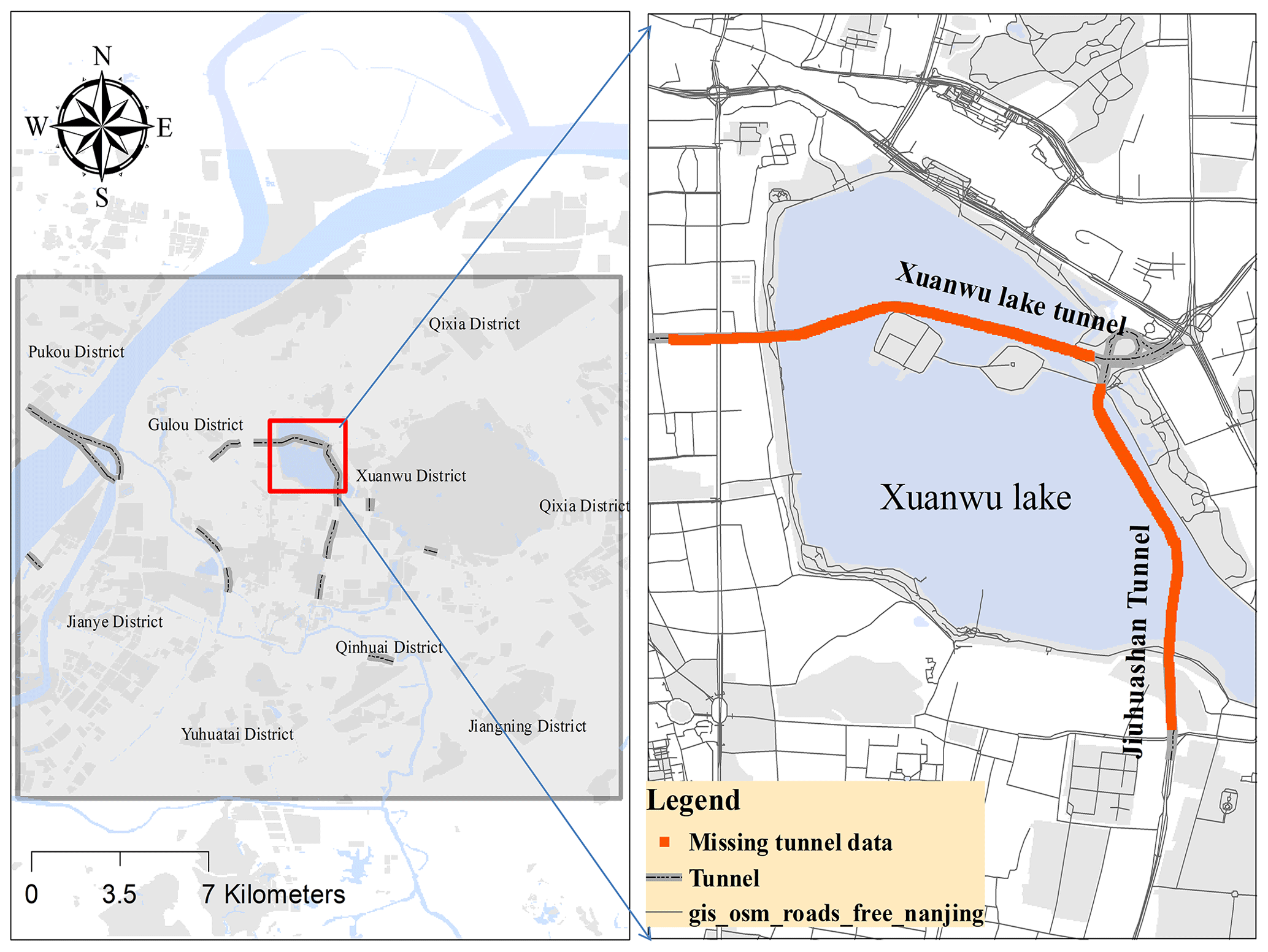
Figure 3Locations of tunnels in Nanjing urban area. © OpenStreetMap contributors 2019. Distributed under a Creative Commons BY-SA License.
2.4 Traffic source attribution
The mobile platform keeps sampling in the urban road network which carries a strong signal from traffic sources. By contrast, stationary stations are often located far away from major roads to represent a regional background air pollution level (Hilker et al., 2019). Seven state-operated air quality observation stations in Nanjing are selected in our research, including Maigaoqiao, Caochangmen, Shanxi Road, Zhonghuamen, Ruijin Road, Xuanwu Lake, and the Olympic Sports Center (Zhao et al., 2015; Zou et al., 2017), which are far away from major roads and large point sources, so they are usually used as regional backgrounds in different functional areas (Zou et al., 2017; An et al., 2015). For example, Zou et al. (2017) chose the Olympic Center station (G in Fig. 1) to get the background characteristics of CO and NO2 in Nanjing. Therefore, the normalized contribution from traffic-related emissions can be obtained by differencing the mobile measurements and the stationary ones to minimize the influence of daily meteorological variations on the urban air quality, following Bossche et al. (2015):
where APtraffic,ij represents the air pollutant concentration contributed by traffic emissions for the ith pollutant at time j (%); APij is the sensor-measured concentration of air pollutants; and APmin means the ambient background concentration, which is calculated as the minimum of the measurements from all the stations in Nanjing in the national air quality network without major sources within a direct vicinity of 50 m (https://quotsoft.net/air/, last access: 1 November 2020, Fig. 1). We refer to this method as the “background site” (BS).
We also adopt a method similar to Apte et al. (2017) for traffic source attribution. This method includes a peak detection algorithm to calculate the contribution of local traffic emission sources to on-road pollutant concentrations. We calculate the mean and minimum of air pollutant concentrations in each grid as the “peak” and “baseline”, respectively. The difference between the two is considered as the contribution from traffic sources. We refer to this method as “peak detection” (PD). MATLAB R2019a is used for such data calculation.
3.1 Effect of spatial resolution on reproducibility
There is a trade-off between the resolution of an air pollutant concentration map and its reproducibility; i.e., high-resolution maps are subject to large randomness due to the limited number of samples in each grid. We investigate the consistency of spatial patterns of different resolution (10–100 m). We calculated the standard error of the means of samples in each grid (SEM) and then averaged the SEM over all grid cells:
where σ and n are the standard deviation and number of samples in each grid, respectively. We find the calculated SEM first decays rapidly with the grid spacing but tends to be in a regime of linear decay after a resolution of approximately 50 m for all the three air pollutants (Fig. 4). Therefore, we choose a resolution of 50 m, which is consistent with previous studies (Bossche et al., 2015; Apte et al., 2017). For example, Bossche et al. (2015) used a spatial resolution of 20–50 m to map urban air quality and identify hotspots. Apte et al. (2017) found that reproducible results (with high precision and low bias) of NO, NO2, and black carbon can be generated by at least 10–25 repetitions in a specific area with 30 m median spatial aggregation.
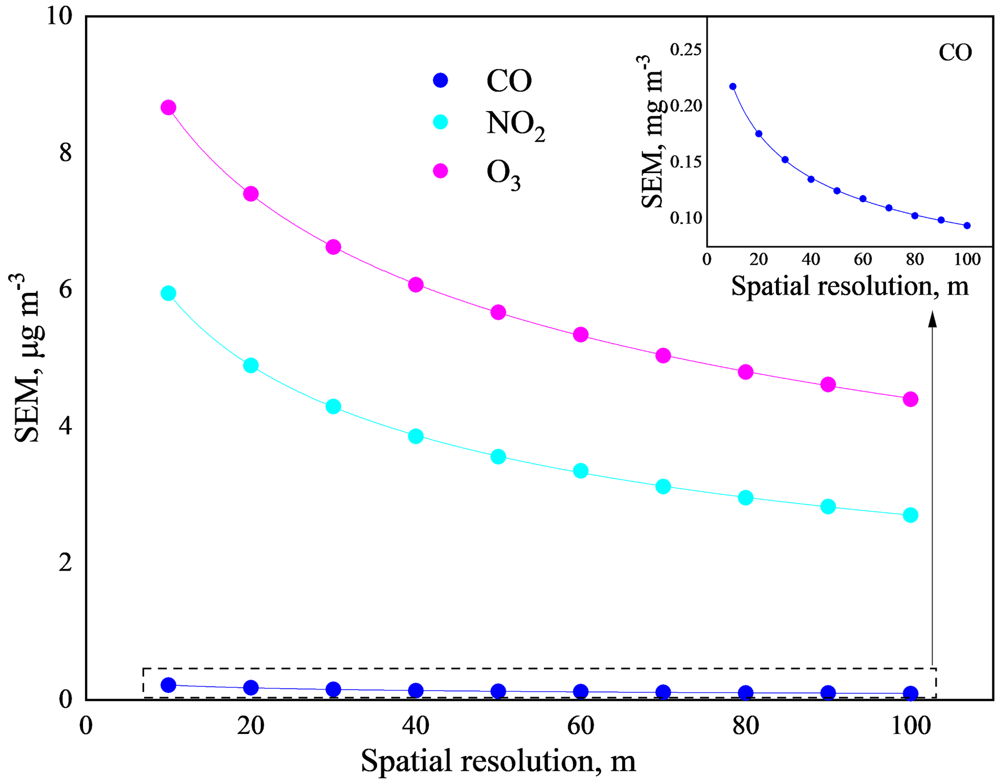
Figure 4Relationship between grid resolution and the domain-averaged standard error of the mean of samples in each grid (SEM) for CO, NO2, and O3.
3.2 Road network coverage
A total of 1.32 million pieces of data were obtained during the observation period, which covers 66.4 % of the major roads in Nanjing in the sampling domain with a large repeat-visit frequency (median repetition = 61 (14 and 264 as the lower and upper quartiles, respectively, the same hereinafter)) (Fig. 5a). The type of road with the most visits is the Neihuan lines (258 (116, 526)), followed by the arterial roads (125 (35, 393)), secondary roads (151 (24, 442)), and highways (34 (12, 115)). The residential streets (22 (6, 100)) have the fewest visits.
Apart from the areas without roads, such as the Yangtze River, Xuanwu Lake, and Purple Mountain, the data cover 43.5 % of the 50 m grids in the research area with the two taxis contributing 36.8 % and 37.2 %. As shown in Fig. 5b, the median number of repeated frequency in each grid is 66 (18, 286), with the highest value of 15 449 in Nanjing South Railway Station and the lowest in some residential roads (1). The repeated frequencies in each 50 m grid along the arterial roads and Neihuan line are higher than other types of roads, i.e., Zhongyang road, Huju road, Neihuandong, and Neihuanxi lines (Fig. 5b). Our repeated frequency is generally higher than previous research on mobile monitoring of urban air pollution (Peters et al., 2013; Poppel et al., 2013; Bossche et al., 2015; Apte at al., 2017), which can lower the uncertainty of our results. By comparing the time series of the air pollutant concentrations with that from nearby state-operated air quality observation stations (A′ and E′, with repeated frequencies > 500), we find that the results are consistent (Fig. S1 in the Supplement), which shows the stability and reliability of our data.
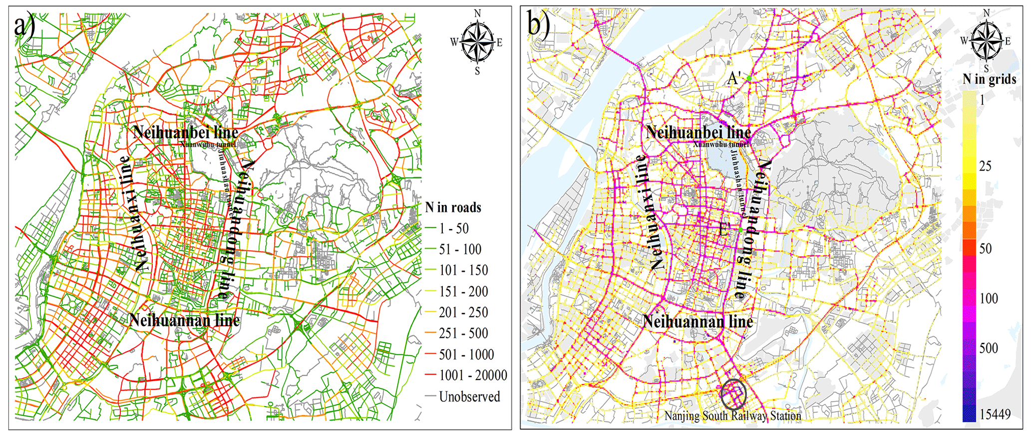
Figure 5Mobile monitoring data coverage with regard to roads (a) and 50 m grids (b). © OpenStreetMap contributors 2019. Distributed under a Creative Commons BY-SA License.
3.3 Variability analysis
Figures 6 and S2 show the coefficients of variation (CV ≡ standard deviation mean × 100 %) for different air pollutants in each grid. For one thing, this matrix quantifies the sensing power of mobile monitoring, i.e., more data points reduce the uncertainty of observations. For another, it reflects the inherent variability of pollutants caused by factors such as meteorological conditions and hotspot emission sources. We find that the CV values are lower than 100 % on the main roads, including highways and arterial roads, but higher than 100 % on some tunnels, residential streets, and Nanjing railway station. As discussed above, the road network coverage is much higher over the main roads than smaller roads. This indicates that increasing the sampling numbers within secondary and residential roads is the most useful way to reduce the uncertainty of mobile observation. It is also interesting to note that a single taxi has a data coverage of ∼ 37 % but the second one only increases it by ∼ 6.5 % to 43.5 %, which implies that the marginal increase in spatial coverage decreases substantially with an increasing number of sensors. This is indeed one limitation of our monitoring platform, and a much larger fleet size or different sampling platforms (e.g., bikes) may be needed to reduce the uncertainty over these smaller roads.
Although the spatial patterns of CV are similar for different air pollutants, we find generally higher CV for O3 (67.3 %) and NO2 (59.5 %) than CO (51.6 %). This is associated with the spatial and temporal variability of different air pollutants, which are influenced by their lifetimes in the atmosphere. Lifetime (or residence time) is the average time for a chemical compound that is transported in the atmosphere before it is deposited or consumed by chemical reactions. It is associated with its spatial scale of variability. The longer the lifetime, the more uniformly the concentrations are distributed. The chemical properties of CO are the most stable in the environment (τ=1–2 months), and its spatial concentration difference is more affected by the sampling time and the number of samples. The lifetime of NOx is shorter (τ=2–11 h, Romer et al., 2016), so the measured concentrations are more influenced by local or “hotspot” emissions and meteorological factors. O3 has the shortest lifetime ( 1 h in urban atmosphere, McClurkin et al., 2013) among the three pollutants. The level of ozone is affected by its precursors (NOx and VOCs), which both have large variability (Sharma et al., 2016). The complex chemical reactions also increase its spatial heterogeneity.
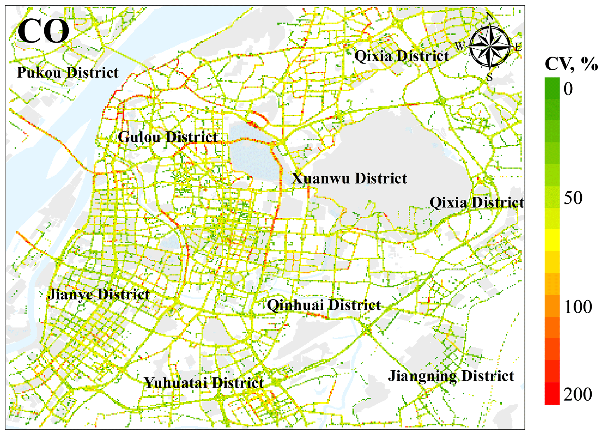
Figure 6Spatial distribution of coefficient of variation for CO in 50 m grids in research domain. © OpenStreetMap contributors 2019. Distributed under a Creative Commons BY-SA License.
3.4 Spatial distribution
3.4.1 Hotspot identification
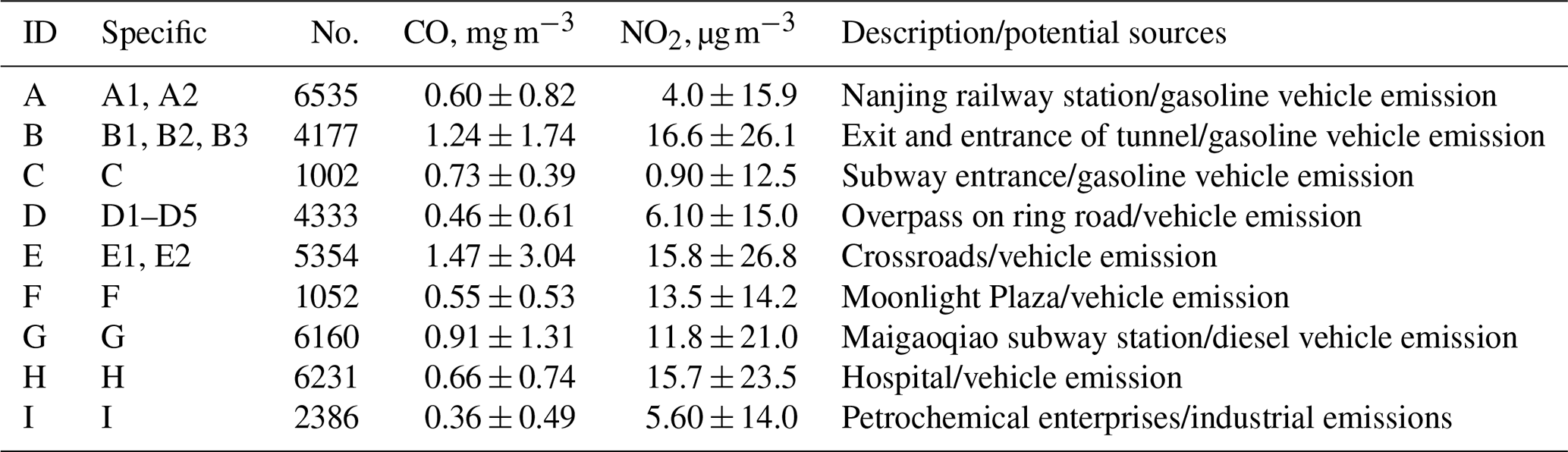
Although the instantaneous pollution level varies drastically in different road environments, we obtain a relatively robust time-integrated pollution estimate by calculating the mean of repeated samples (Fig. 7). We define the area where the pollutant concentrations are 50 % higher than nearby grids (radius = 300 m) as “hotspots” following Apte et al. (2017). The pollutant concentrations shown in Table 1 are the values after deducting the background concentration, which are calculated by the annual mean concentration of stationary stations. A total of 17 hotspots for CO and NO2, and 17 hotspots for O3 are identified, and the specific information is shown in Fig. 7 and Table 1. Most of the “hotspots” show relatively apparent spatial “peaks” for multiple pollutants. To identify the main sources contributing to these hotspots, we use the different relative concentrations of the measured pollutants (Zhao et al., 2015). We also use field information around hotspot areas, such as the existence of subway stations, construction sites, factories, and restaurants nearby. This method has substantial uncertainties in terms of the attribution of the potential sources to these “hotspots”, and further source–receptor relationships and detailed chemical component analyses are required to identify the exact emission sources.
We find that “hotspots” are mainly affected by one of the three types of emission sources, namely traffic emissions (diesel and gasoline on-road vehicle exhaust), industrial emissions, and cooking fumes. The mean CO and NO2 concentrations are relatively high at the crossroads (E, 1.47 mg m−3 and 15.8 µg m−3), tunnels (B, 1.24 mg m−3 and 16.6 µg m−3, respectively), the roads near the hospital (H, 0.66 mg m−3 and 15.7 µg m−3), and near the railway station (A, 0.60 mg m−3 and 4.0 µg m−3), which are affected by on-road traffic emissions. In addition, due to the construction of Maigaoqiao subway station (G, 0.91 mg m−3 and 11.8 µg m−3), diesel vehicles and off-road traffic emission also make a great contribution to CO and NO2 concentrations. Industrial emissions from petrochemical enterprises (I) also lead to high NO2 concentrations (0.26–93.1 µg m−3) on surrounding roads.
As shown in Fig. 7, the higher O3 concentrations in these hotspot areas are mainly caused by higher NOx and VOC emissions from the heavy traffic (W, 46.8 ± 27.4 µg m−3; Xie et al., 2016; Ding et al., 2013), cooking emissions (Q, 38.5 ± 26.0 µg m−3), and ozone precursors from industrial emissions (e.g., K, 47.1 ± 36.5 µg m−3, and J, 37.6 ± 25.8 µg m−3), such as VOCs. In addition, biogenic VOC emissions also have a significant impact on the formation of ozone (U, 40.4 ± 18.3 µg m−3, and V, 33.5 ± 20.4 µg m−3; Liu et al., 2018). Taxi sensor data also reveal the secondary pollution characteristics at the micro-scale, showing that O3 concentration in the downtown area with dense buildings is significantly higher than that in other areas, especially some residential areas in Jianye and Gulou district. Previous studies have also found that the air pollutant “hotspots” are associated with traffic-related emissions (e.g., heavy-duty diesel vehicles, Targino et al., 2016, and vehicle congestion, Gately et al., 2017) and high-density urban areas (Li et al., 2018). These identified air pollution “hotspots”, and the diagnosed source contributions provide helpful information for urban air quality management, which demonstrates the sensing power of mobile monitoring deployed on a taxi fleet.
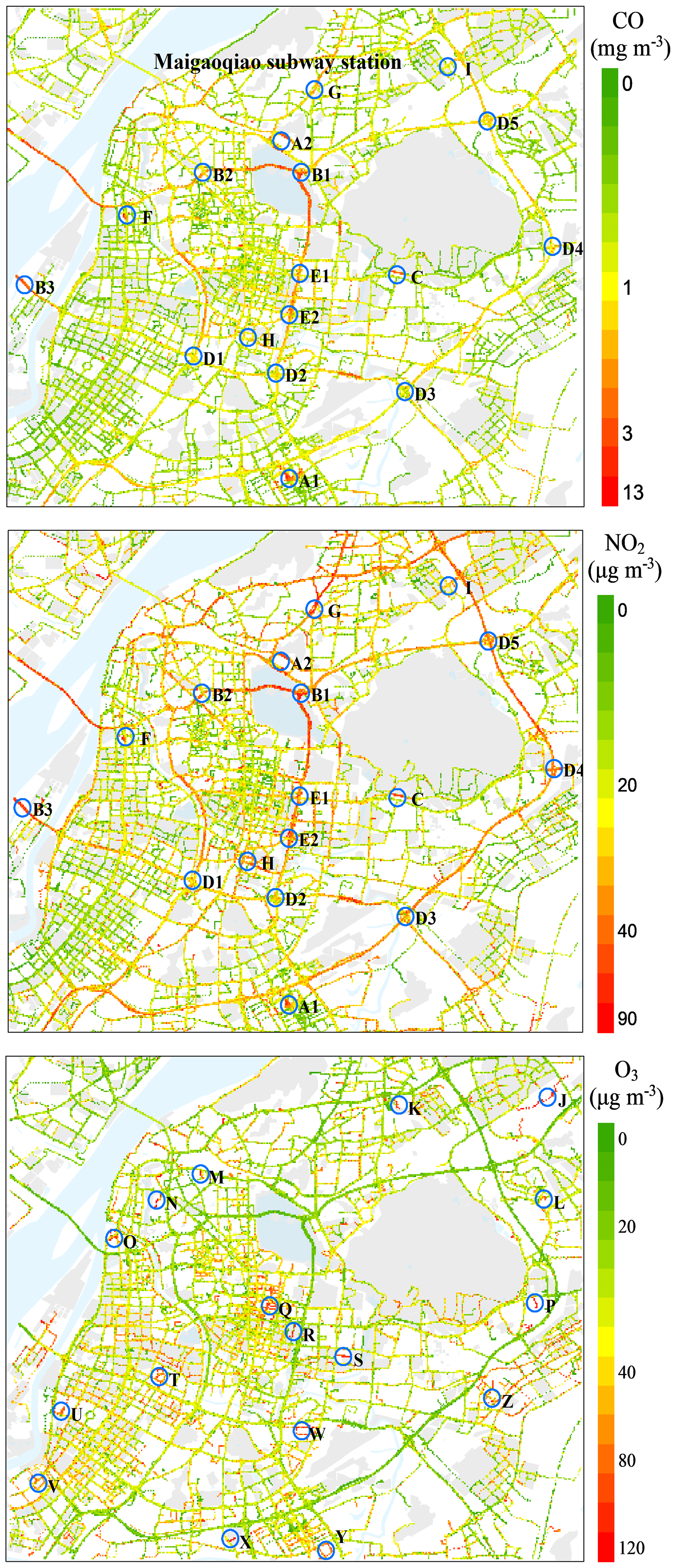
Figure 7Spatial distribution and “hotspots” of air pollutant concentrations in the research domain (CO, NO2, and O3). Circles marked with A–Z represent the identified “hotspots”, where the air pollutant concentrations are at least 50 % higher than the surrounding area (300 m radius). © OpenStreetMap contributors 2019. Distributed under a Creative Commons BY-SA License.
Table 1“Hotspots” of air pollution for multi-pollutants identified in Nanjing. “No.” refers to the number of observation points within 300 m of the hotspots.
3.4.2 Air pollutant concentrations in different types of roads
We find that air pollutant levels differ vastly among the six types of roads (p<0.05, with the ANOVA method). The mean CO and NO2 concentrations follow this trend: tunnels (2.22 ± 1.18 mg m−3 and 40.7 ± 29.7 µg m−3, respectively) > highways (1.10 ± 0.59 mg m−3 and 29.2 ± 8.66 µg m−3) > arterial roads (0.958 ± 0.308 mg m−3 and 25.0 ± 6.90 µg m−3) > secondary roads (0.855 ± 0.401 mg m−3 and 21.8 ± 8.89 µg m−3) > branch roads (0.818 ± 0.216 mg m−3 and 20.3 ± 6.79 µg m−3) > residential streets (0.783 ± 0.299 mg m−3 and 19.7 ± 8.35 µg m−3) (Table 2). However, the mean O3 concentrations in different types of roads are opposite to that of CO and NO2: residential streets (35.1 ± 15.4 µg m−3) > branch roads (32.7 ± 12.2 µg m−3) > secondary roads (31.9 ± 10.0 µg m−3) > arterial roads (29.6 ± 7.52 µg m−3) > highways (23.3 ± 9.12 µg m−3) > tunnels (15.7 ± 7.85 µg m−3).
The differences of air pollutant concentrations among different road types are firstly affected by the traffic-related emission sources including vehicle engine exhaust, which is a function of traffic flow and speed, vehicle type, etc. (Sahanavin et al., 2018). The general decreasing trends we observed for CO and NO2 are consistent with traffic flow and the congestion index in the Nanjing urban area (Table 2, Zou et al., 2017). Apte et al. (2017) also found that the NO2 concentration decreased in turn on highways, arterial roads, and residential streets, which are in good agreement with our research. The observed O3 concentrations have opposite trends of CO and NO2 with the highest concentration in residential streets (Table 2). As O3 production in Nanjing is in VOC-limited regions, lower NOx could reduce its titration of O3 and subsequently increase O3 concentration (Ding et al., 2013; Xie et al., 2016). The O3 concentrations are lowest in tunnels, which is associated with the weak sunlight in the tunnels (Awang et al., 2015). Furthermore, due to the unfavorable diffusion conditions in the tunnels, NO2 concentration is accumulated to a relatively high level (40.7 ± 29.7 µg m−3), which titrates O3. The tunnel also blocks the replenishment of surrounding O3-rich air, resulting in a lower O3 concentration than other roads (Kirchstetter et al., 1996).
Table 2Multi-pollutant concentrations for six types of roads.
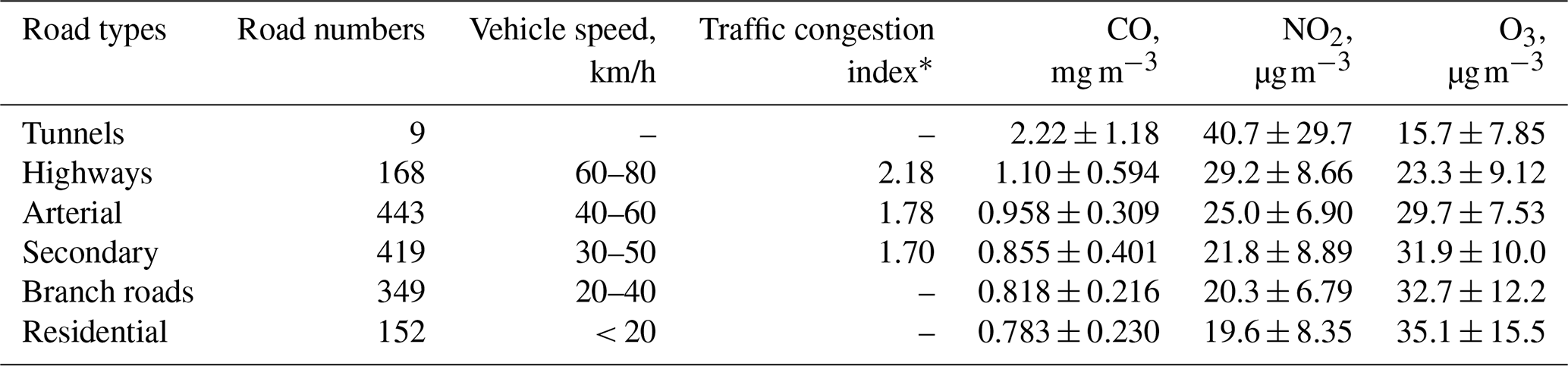
* The traffic congestion index data are from the Gaud map https://report.amap.com/detail.do?city=320100 (last access: 24 October 2020).
3.5 Temporal variation
Figure 8 shows the temporal variation of the three air pollutant concentrations during the observation campaign, with the hourly mean concentrations over the research domain shown in Fig. 9 (the corresponding spatial distributions are shown in Figs. S4–6). The difference of the hourly variation of the mean sample of different types of roads over a year is small (Fig. S7), so the data in Fig. 9 are not filtered in anyway, but for each hour a similar mix of road types is sampled. We find that the median concentrations of CO and NO2 in rush hours (07:00–09:00 and 17:00–19:00 LT) are increased by 26.4 % and 27.3 % compared to non-rush hours, respectively. The hourly mean concentrations of CO and NO2 show a double-peak pattern with higher concentrations in rush hours (Fig. 9a), reflecting the contribution of traffic-related emissions (Tan et al., 2009), which we will elaborate in the next section. The observed O3 concentrations show a unimodal diurnal pattern with a peak at ∼ 14:00 LT as a result of photochemical formation. At night, O3 concentrations are maintained at a low level due to a lack of solar radiation and the NOx-titration effect (Xie et al., 2016; Li et al., 2013). These patterns generally agree with the measurements at stationary monitoring stations (Fig. S3).
No significant differences are observed for the median concentrations and spatial distribution of three air pollutants between weekdays and weekends (α=0.05; Figs. 8b and S4), even though the morning peaks for CO are slightly higher during weekdays (Fig. 9b), which is consistent with An et al. (2015). Wang et al. (2014) found that NOx displays a weekly cycle in the Beijing–Tianjin–Hebei metropolitan area, with higher levels on weekdays than weekends. Qin et al. (2004) observed a significant weekend effect in southern California, showing that during the morning traffic rush hour, the concentrations of CO and NO2 at weekends were about 18 % and 37 % lower than on weekdays. The difference between our study and other cities lies in the difference of fleet fuel structure, and the different weekly routine of human activities and the taxi driving trajectories (Xie et al., 2016).
The median concentrations of CO and NO2 during holidays are comparable to those during non-holidays but are 18.3 % lower for O3 (Fig. 8c). In addition, compared with the spatial distribution of O3 concentration during holidays, we find that the concentrations of O3 in Xinjiekou and its surrounding areas, where many shopping malls are located, are higher during non-holidays (Fig. S6). This may be related to the higher NO2 concentrations in this area during holidays (24.8 ± 10.2 µg m−3) than non-holidays (20.6 ± 4.82 µg m−3). The hourly concentrations show no significant difference between holidays and non-holidays (Fig. 9c). The holidays include the periods of National Day (1–7 October), the Spring Festival (24–31 February), Qingming Festival (4–6 April), international labor day (1–5 May), and the Dragon Boat Festival (25–27 June). The “holiday effect” has been observed extensively for urban and regional air quality. For example, Xu et al. (2017) found that VOC tracers were significantly enhanced during the National Day holiday (from 1–10 October 2014) in the Yangtze River Delta (YRD) region, indicating that the “holiday effect” had a strong influence on the distribution and chemical reactivity of VOCs in the atmosphere. The reason why this effect is not observed in our study may be related to the relatively smaller sample size during holidays. The sample size for holidays account for only 11.3 % of those for the non-holidays.
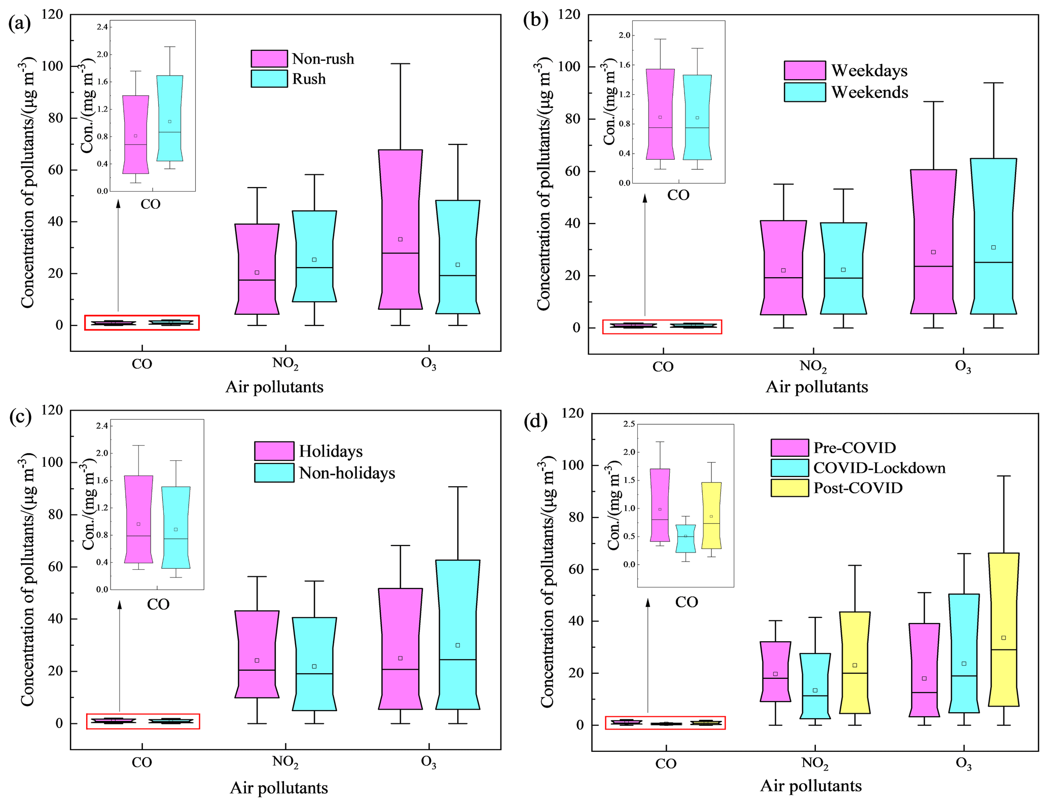
Figure 8Variation of pollutants concentrations in rush/non-rush hours, weekdays/weekend days, holidays/non-holidays, and three stages of the COVID-19 pandemic. The dot in each box represents the mean value and the solid line represents the median value. Each box extends from the 25th to the 75th percentile. The whiskers (error bars) below and above the boxes represents the 10th and 90th percentiles.
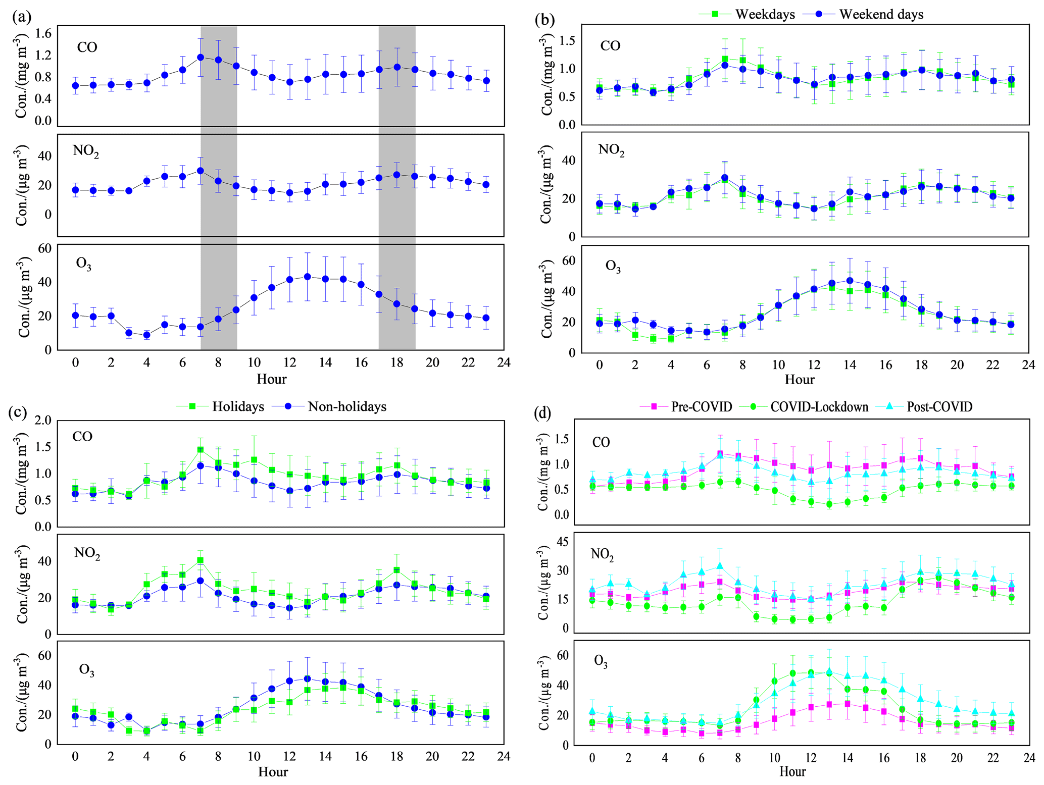
Figure 9Diurnal cycles of three pollutants concentrations measured in rush/non-rush hours, weekdays/weekend days, holidays/non-holidays, and different stage of the COVID-19 pandemic by the taxi sensors. Error bars in panel a show the standard deviation of observations. Gray areas represent the rush hours, and the other represents the non-rush hours (a).
3.6 Traffic source contribution
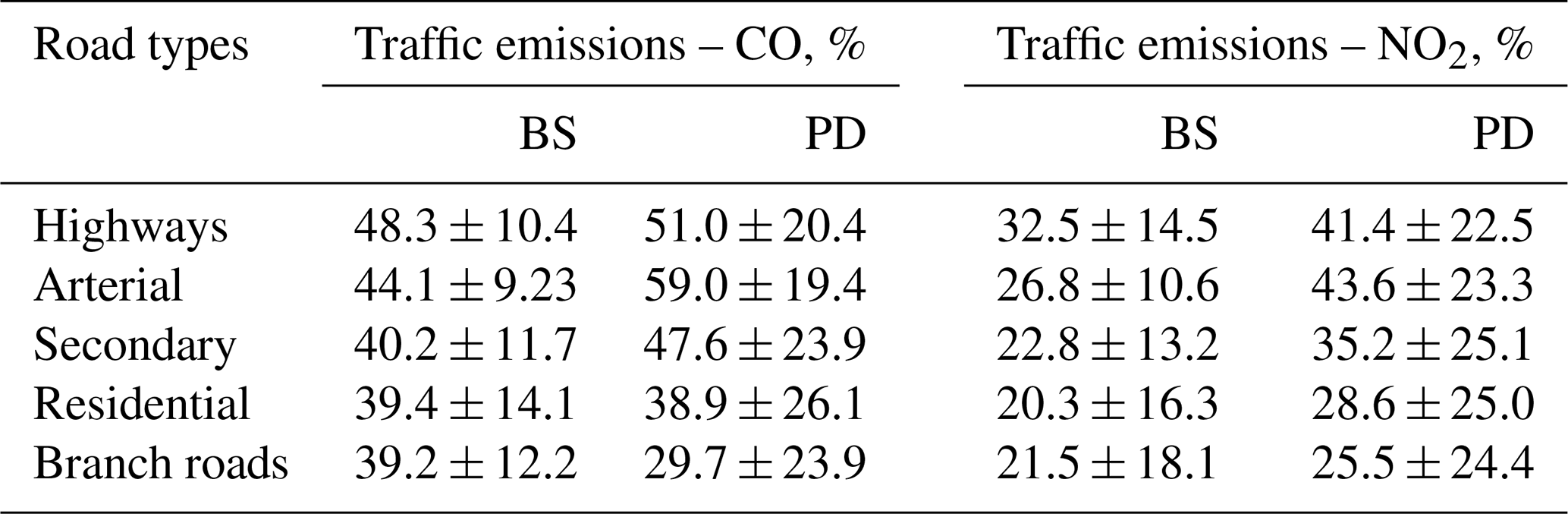
Figure 10a and b show the calculated contributions by traffic-related emission sources to the observed concentration of CO (referred to as contributions hereinafter). We find that the mean contribution calculated by the BS method (42.6 ± 11.5 %) is generally consistent with that obtained from the PD algorithm (43.9 ± 27.0 %). Their spatial patterns are also similar (Fig. 10a vs. b). Although our data coverage is much larger than that of the Apte et al. (2017) study, we find that the reference method is still applicable in our research area. The contributions in highways, near tunnel entrances and exits (e.g., Jiuhuashan and Xuanwuhu tunnel), at the railway station (Nanjing south station), and on arterial roads (44 %–59 %) calculated using both methods are higher than on secondary roads and residential streets and lowest on branch roads (29 %–39 %) (Table 3), which is consistent with the trend in traffic volumes. The patterns for NO2 are quite similar to CO (Fig. S8c and d, Table 1), but the mean contribution to NO2 calculated using the BS method (26.3 ± 14.7 %) is lower than that obtained from the PD algorithm (40.2 ± 29.9 %). This difference is associated with the relatively higher uncertainty for NO2 measurements by sensors (Sect. 2.2), while the results of the PD method seem unaffected as the sensor bias is canceled out when calculating the difference between “peak” and “baseline” (Sect. 2.4).
The bottom-up emission inventory indicates that on-road transportation contributed ∼ 11 % of total CO emissions from Nanjing in 2012 (Zhao et al., 2015). Considering the number of cars has increased by ∼ 80 % and the total CO emissions remained relatively stable (BSNM, 2019), the contribution of traffic sources in recent years is expected to be ∼ 20 %. These values are much lower than what we calculated based on mobile monitoring data because of the lower spatial resolution of these regional inventories (e.g., 0.05∘ × 0.05∘) (Zheng et al., 2014). They are unable to distinguish the emission characteristics of air pollutant within a street level (tens of meters), which leads to their underestimation of traffic-related emissions in the road micro-environment.
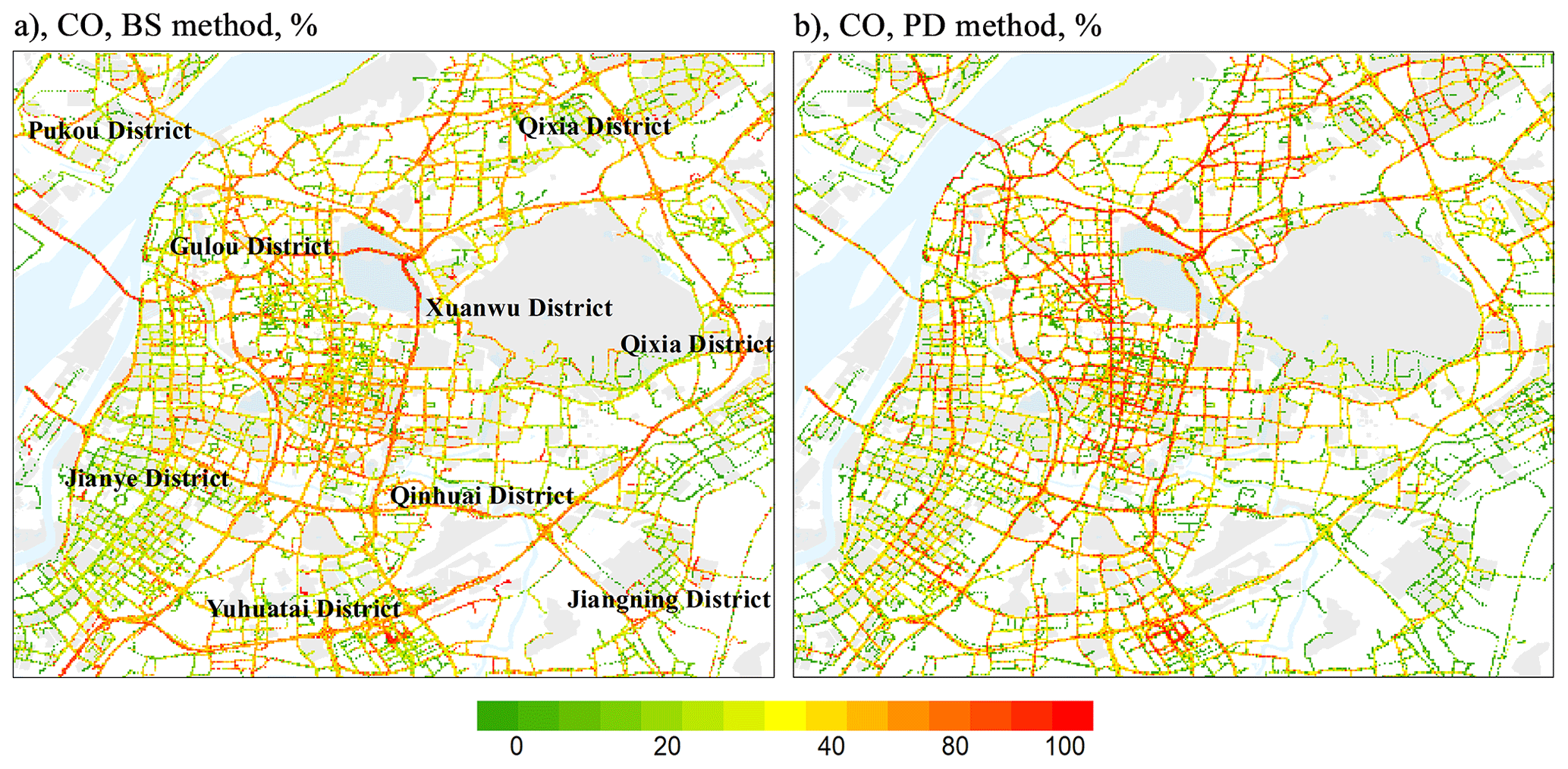
Figure 10Contributions from traffic-related emissions calculated using the stationary data method (a) and peak detection algorithm (b) for CO. © OpenStreetMap contributors 2019. Distributed under a Creative Commons BY-SA License.
Table 3Contribution of traffic emissions to CO and NO2 in different roads using the two methods.
3.7 Impact of COVID-19 pandemic
Figures 8d and 9d show the variation of air pollutant concentrations at different stages of the COVID-19 pandemic. The spatial distribution of concentrations and traffic contributions are also depicted in Figs. 11–12 and S9–S10. We divide the data into three stages: pre-COVID (P1, 1 October 2019–23 January 2020), COVID lockdown (P2, 24–31 January 2020 and 17–24 February 2020), and post-COVID (P3, 1 March–30 September 2020). We find the median concentrations of CO and NO2 were the lowest in P2 (Fig. 9d). For example, the CO and NO2 concentrations decreased by 44.9 % and 41.7 % from P1 to P2, respectively (Figs. 11 and S8). This pattern agrees well with the air quality station data over eastern China (Huang et al., 2021). We focus on the traffic sector as it is the most sensitive to lockdown measures, while other sectors, including power, industrial, and residential sectors, remain relatively unchanged (Guevara et al., 2021). We find that from P1 to P2, the average traffic source contributions of CO and NO2 using the BS method decreased by 59.9 % and 51.8 %, respectively (Figs. 12 and S9). This is consistent with the transportation index data, which shows a 70 % reduction in eastern Chinese cities during lockdown (Huang et al., 2021).
The observed CO and NO2 concentrations recovered to a level similar to P1 during P3. The traffic-related source contributions were increased by 120 % and 131 % from P2 to P3 for CO and NO2 (Figs. 11 and S9). Due to the limited data size and spatial coverage (only on some arterial roads and highways) during P2, the calculated contribution of traffic emissions to air pollutants may be not directly comparable to those shown in Fig. 9. But the changes in the contribution match well with the changes in traffic volume and human activities (Bao and Zhang, 2020). Our results also agree with top-down emission estimates from remote sensing data (Zhang et al., 2020), which showed the total NO2 emissions decreased by 31 %–44 % from P1 to P2 but increased 67 %–85 % from P2 to P3.
The observed ozone concentrations show a different trend from other pollutants in the three stages. We find a pattern of P1 < P2 < P3 for O3 median concentrations (Fig. 8d). The ozone concentration increased by 35.7 % from P1 to P2, and 48.7 % from P2 to P3 (Fig. S9). While the contribution of traffic emissions to ozone first decreased by 32.5 % from P1 to P2 and then increased by 39.3 % in P2 to P3 (Fig. S10). This is firstly associated with less titration of NOx during P2 as discussed earlier. In addition, the increased temperature and solar insolation in P2 and P3 also favor the photochemical formation of O3 compared to P1 (Xie et al., 2016; Fu et al., 2015; Reddy et al., 2010).
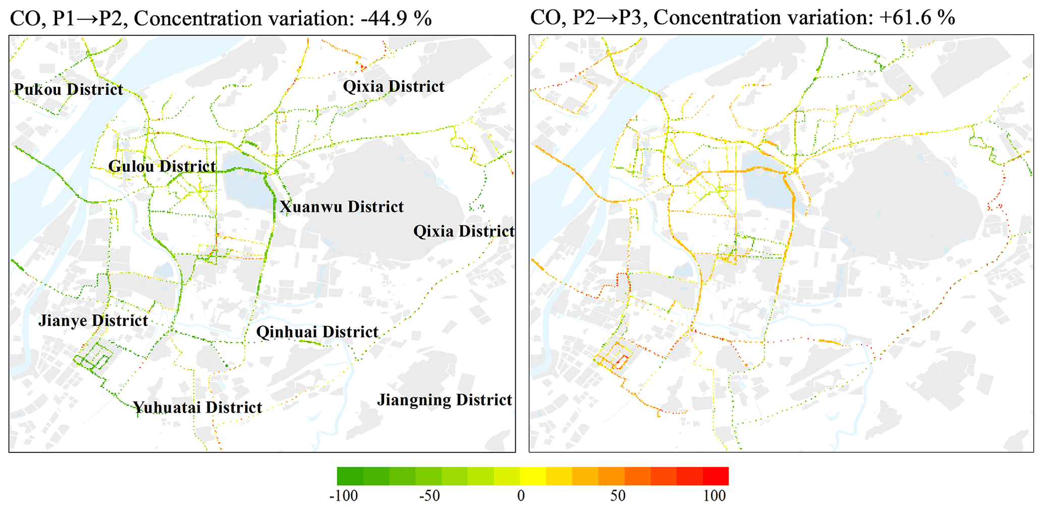
Figure 11Changes in observed CO concentration in the three stages of the COVID-19 pandemic. P1, P2, and P3 are for pre-COVID, COVID-lockdown, and post-COVID periods, respectively. © OpenStreetMap contributors 2019. Distributed under a Creative Commons BY-SA License.
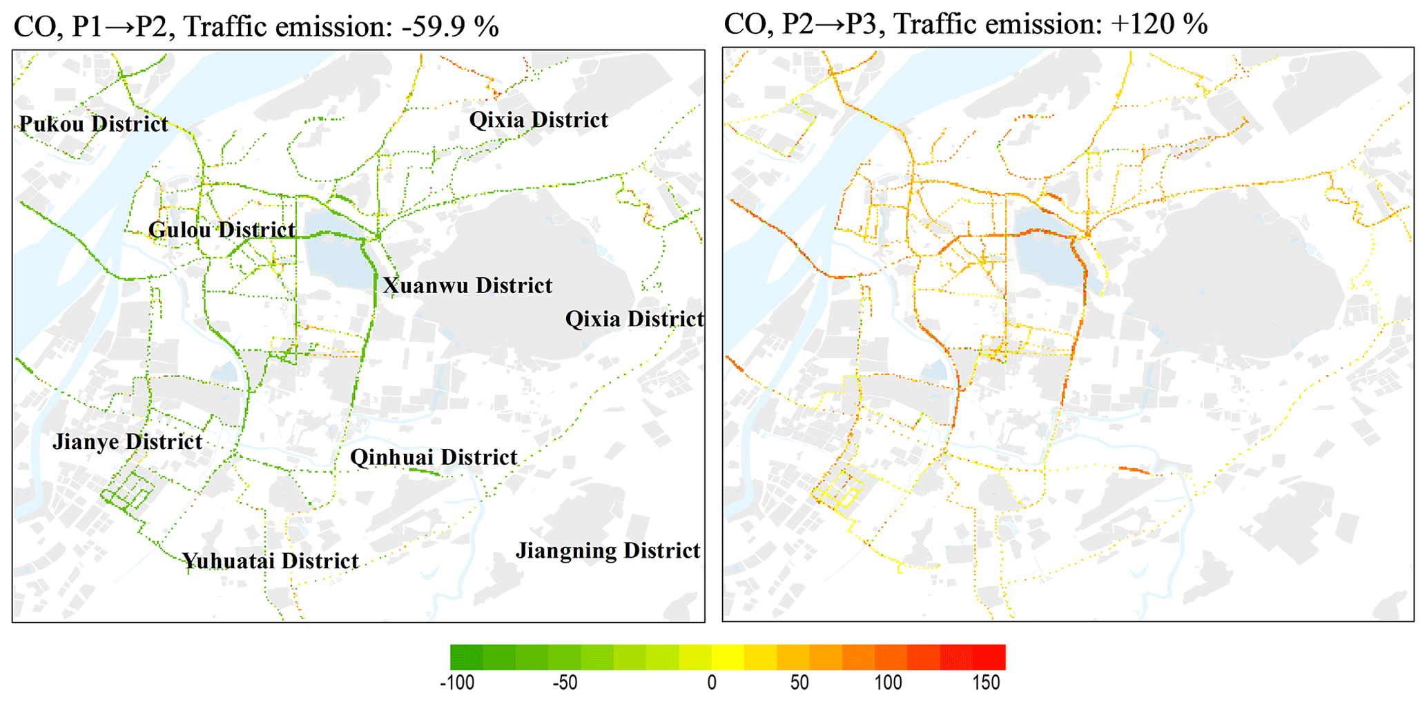
Figure 12Changes in the contributions of traffic-related sources to CO in the three stages of the COVID-19 pandemic calculated using the BS method. P1, P2, and P3 are for pre-COVID, COVID-lockdown, and post-COVID periods, respectively. © OpenStreetMap contributors 2019. Distributed under a Creative Commons BY-SA License.
Accurate assessment of human exposure to urban air pollution requires a detailed understanding of the spatial and temporal patterns of air pollutant concentrations. Combining mobile monitoring with GIS technology, we obtained high-resolution (50 m × 50 m) spatial distribution maps of three air pollutants in the main urban area of Nanjing, which demonstrates well the spatial heterogeneity of pollutants at the micro-scales. We find that higher spatial resolution is useful to identify hotspots that are mainly affected by three types of air pollution emissions sources, namely, traffic, industrial, and cooking fumes. It also provides hints for air quality management and emission source control.
We calculate the contribution of traffic-related emissions to air pollutants in different grid points by combining mobile observation and station observation data. Compared with the peak detection method, the station data method is more reasonable for secondary pollutants such as O3, while the former is less affected by sensor bias. There are also some differences in the contribution of traffic emissions to air pollutants in different types of roads. Due to the impact of the COVID-19 pandemic, the mean concentrations of CO and NO2 decreased by 44.9 % and 47.1 %, respectively, during the lockdown in Nanjing, and the contribution of traffic-related emissions also decreased by 59.9 % and 52.6 %. In contrast, the concentration of O3 increased by 35.7 %, respectively. After reopening, CO and NO2 concentrations rebounded by 61.6 % and 48.2 %, and the contribution of traffic emissions both increased by over 100 %, indicating the great impact of traffic emissions on urban air pollution.
All validation data and data processing by GIS used in this work can be accessed by contacting the authors.
The supplement related to this article is available online at: https://doi.org/10.5194/acp-21-7199-2021-supplement.
YZ designed the research. SW performed the research. SW, YZ, ZW, and MY analyzed data. LW, XC, and AD provided validation data. MY, YL, and QL helped with the data analysis. MW, LZ, and YX provided the monitoring instrument. SW and YZ wrote the paper.
The authors declare that they have no conflict of interest.
This article is part of the special issue “Air Quality Research at Street-Level (ACP/GMD inter-journal SI)”. It is not associated with a conference.
We are grateful to the Station for Observing Regional Processes of the Earth System (SORPES) in Xianlin Campus of Nanjing University for providing the background data for sensor calibration. The authors thank Rong Ye and Liang Luo for sample collection.
This study was supported by the National Key Research & Development Program of China (grant nos. 2016YFC0202000 and 2019YFA0606803), Jiangsu Innovative and Entrepreneurial Talents Plan, and the Collaborative Innovation Center of Climate Change, Jiangsu Province.
This paper was edited by Joel Thornton and reviewed by three anonymous referees.
An, J. L., Zou, J., Wang, J., Lin., X., and Zhu, B.: Differences in ozone photochemical characteristics between the megacity Nanjing and its suburban surroundings, Yangtze River Delta, China, Environ. Sci. Pollut. Res., 22, 19607–19617, https://doi.org/10.1007/s11356-015-5177-0, 2015.
Apte, J. S., Kirchstetter, T. W., Reich, A. H., Deshpande, S. J., Kaushik, G., Chel, A., Marshall, J. D., and Nazaroff, W. W.: Concentrations of fine, ultrafine, and black carbon particles in auto-rickshaws in New Delhi, India, Atmos. Environ., 45, 4470–4480, https://doi.org/10.1016/j.atmosenv.2011.05.028, 2011.
Apte, J. S., Messier, K. P., Gani, S., Brauer, M., Kirchstetter, T. W., Lunden, M. M., Marshall, J. D., Portier, C. J., Vermeulen, R. C. H., and Hamburg, S. P.: High-resolution air pollution mapping with google street view cars: exploiting big data, Environ. Sci. Technol., 51, 6999–7008, https://doi.org/10.1021/acs.est.7b00891, 2017.
Awang, N. R., Ramli, N. A., Yahaya, A. S., and Elbayoumi, M.: High nighttime ground-level ozone concentrations in Kemaman: NO and NO2 concentrations attributions, Aerosol Air Qual. Res., 15, 1357–1366, https://doi.org/10.4209/aaqr.2015.01.0031, 2015.
Bao, R. and Zhang, A.: Does lockdown reduce air pollution? Evidence from 44 cities in northern China, Sci. Total Environ., 139052, https://doi.org/10.1016/j.scitotenv.2020.139052, 2020.
Bart, E., Jan P., Martine, V. P., Nico, B., and Arnout, S.: The aeroflex: a bicycle for mobile air quality measurements, Sensors, 13, 221–240, https://doi.org/10.3390/s130100221, 2012.
Boogaard, H., Kos, G. P. A., Weijers, E. P., Janssen, N. A. H., Fischer, P. H., Van der Zee, S. C., De Hartog, J. J., and Hoek, G.: Contrast in air pollution components between major streets and background locations: Particulate matter mass, black carbon, elemental composition, nitrogen oxide and ultrafine particle number, Atmos. Environ., 45, 650–658, https://doi.org/10.1016/j.atmosenv.2010.10.033, 2010.
Borrego, C., Coutinho, M., Costa, A. M., Ginja, J., Ribeiro, C., Monteiro, A., Ribeiro, I., Valente, J., Amorim, J. H., Martins, H., Lopes, D., and Miranda, A. I.: Challenges for a new air quality directive: the role of monitoring and modelling techniques, Urban Clim., 14, 328–341, https://doi.org/10.1016/j.uclim.2014.06.007, 2015.
Bossche, J. V. D., Peters, J., Verwaeren, J., Botteldooren, D., Theunis, J., and Baets, B. D.: Mobile monitoring for mapping spatial variation in urban air quality: Development and validation of a methodology based on an extensive dataset, Atmos. Environ., 105, 148–161, https://doi.org/10.1016/j.atmosenv.2015.01.017, 2015.
Bureau Statistics of Nanjing Municipal: Nangjing Statistical Yearbook, available at: http://tjj.nanjing.gov.cn/bmfw/njsj/ (last access: 8 November 2020), 2019.
Castell, N., Dauge, F. R., Schneider, P., Vogt, M., Lerner, U., Fishbain, B., Broday, D., and Bartonova, A.: Can commercial low-cost sensor platforms contribute to air quality monitoring and exposure estimates?, Environ. Int., 99, 293–302, https://doi.org/10.1016/j.envint.2016.12.007, 2017.
Cavellin, L. D., Weichenthal, S., Tack, R., Ragettli, M. S., Smargiassi, A., and Hatzopoulou, M.: Investigating the use of portable air pollution sensors to capture the spatial variability of traffic-related air pollution, Environ. Sci. Technol., 50, 313–320, https://doi.org/10.1021/acs.est.5b04235, 2016.
Chatzidiakou, L., Krause, A., Popoola, O. A. M., Di Antonio, A., Kellaway, M., Han, Y., Squires, F. A., Wang, T., Zhang, H., Wang, Q., Fan, Y., Chen, S., Hu, M., Quint, J. K., Barratt, B., Kelly, F. J., Zhu, T., and Jones, R. L.: Characterising low-cost sensors in highly portable platforms to quantify personal exposure in diverse environments, Atmos. Meas. Tech., 12, 4643–4657, https://doi.org/10.5194/amt-12-4643-2019, 2019.
Ding, A. J., Fu, C. B., Yang, X. Q., Sun, J. N., Zheng, L. F., Xie, Y. N., Herrmann, E., Nie, W., Petäjä, T., Kerminen, V.-M., and Kulmala, M.: Ozone and fine particle in the western Yangtze River Delta: an overview of 1 yr data at the SORPES station, Atmos. Chem. Phys., 13, 5813–5830, https://doi.org/10.5194/acp-13-5813-2013, 2013.
Esposito, E., Vito, S. D., Salvato, M., Fattoruso, G., Bright, V., Jones, R. L., and Popoola, O.: Stochastic Comparison of Machine Learning Approaches to Calibration of Mobile Air Quality Monitors, in: Sensors, CNS 2016, Lecture Notes in Electrical Engineering, edited by: Andò, B., Baldini, F., Di Natale, C., Marrazza, G., Siciliano, P., vol 431, Springer, Cham, https://doi.org/10.1007/978-3-319-55077-0_38, 2018.
Farrell, W. J., Cavellin, L. D., Weichenthal, S., Goldberg, M., and Hatzopoulou, M.: Capturing the urban canyon effect on particle number concentrations across a large road network using spatial analysis tools, Build. Environ., 92, 328–334, https://doi.org/10.1016/j.buildenv.2015.05.004, 2015.
Fu, T. M., Zheng, Y., Paulot, F., and Mao, J.: Positive but variable sensitivity of August surface ozone to large-scale warming in the southeast United States, Nat. Clim. Change, 5, 454–458, https://doi.org/10.1038/nclimate2567, 2015.
Gately, C. K., Hutyra, L. R., Peterson, S., and Wing, I. S.: Urban emissions hotspots: Quantifying vehicle congestion and air pollution using mobile phone GPS data, Environ. Pollut., 229, 496–504, https://doi.org/10.1016/j.envpol.2017.05.091, 2017.
Guevara, M., Jorba, O., Soret, A., Petetin, H., Bowdalo, D., Serradell, K., Tena, C., Denier van der Gon, H., Kuenen, J., Peuch, V.-H., and Pérez García-Pando, C.: Time-resolved emission reductions for atmospheric chemistry modelling in Europe during the COVID-19 lockdowns, Atmos. Chem. Phys., 21, 773–797, https://doi.org/10.5194/acp-21-773-2021, 2021.
Hagan, D. H., Gani, S., Bhandari, S., Patel, K., Habib, G., Apte, J. S., Ruiz, L. H., and Kroll, J. H.: Inferring aerosol sources from low-cost air quality sensor measurements: a case study in Delhi, India, Environ. Sci. Tech. Let., 6, 467–472, https://doi.org/10.1021/acs.estlett.9b00393, 2019.
Hasenfratz, D., Saukh, O., Walser, C., Hueglin, C., Fierz, M., Arn, T., Beutel, J., and Thiele, L.: Deriving high-resolution urban air pollution maps using mobile sensor nodes, Pervasive Mob. Comput., 16, 268–285, https://doi.org/10.1016/j.pmcj.2014.11.008, 2015.
Herrmann, E., Ding, A. J., Petäjä, T., Yang, X. Q., Sun, J. N., Qi, X. M., Manninen, H., Hakala, J., Nieminen, T., Aalto, P. P., Kerminen, V.-M., Kulmala, M., and Fu, C. B.: New particle formation in the western Yangtze River Delta: first data from SORPES-station, Atmos. Chem. Phys. Discuss., 13, 1455–1488, https://doi.org/10.5194/acpd-13-1455-2013, 2013.
Hilker, N., Wang, J. M., Jeong, C.-H., Healy, R. M., Sofowote, U., Debosz, J., Su, Y., Noble, M., Munoz, A., Doerksen, G., White, L., Audette, C., Herod, D., Brook, J. R., and Evans, G. J.: Traffic-related air pollution near roadways: discerning local impacts from background, Atmos. Meas. Tech., 12, 5247–5261, https://doi.org/10.5194/amt-12-5247-2019, 2019.
Huang, X., Ding, A. J., Gao, J., Zheng, B., Zhou, D. R., Qi, X., Tang, R., Wang, J., Ren, C., Nie, W., Chi, X., Xu, Z., Chen, L., Li, Y., Che, F., Pang, N., Wang, H. K., Tong, D., Qin, W., Cheng, W., Liu, W., Fu, Q., Liu, B., Chai, F. H., Davis, S. J., Zhang, Q., and He, K. B.: Enhanced secondary pollution offset reduction of primary emissions during COVID-19 lockdown in China, Natl. Sci. Rev., 8, 1–9, https://doi.org/10.1093/nsr/nwaa137, 2021.
Isakov, V., Touma, J. S., and Khlystov, A.: A method of assessing air toxics concentrations in urban areas using mobile platform measurements, J. Air Waste Manage. Assoc., 57, 1286–1295, https://doi.org/10.3155/1047-3289.57.11.1286, 2007.
Ivanovskaya, M., Gurlo, A., and Bogdanov, P.: Mechanism of O3 and NO2 detection and selectivity of In2O3 sensors, Sensor Actuat. B-Chem., 77, 264–267, https://doi.org/10.1016/S0925-4005(01)00708-0, 2001.
Johnson, N. E., Bonczak, B., and Kontokosta, C. E.: Using a gradient boosting model to improve the performance of low-cost aerosol monitors in a dense, heterogeneous urban environment, Atmos. Environ., 184, 9–16, https://doi.org/10.1016/j.atmosenv.2018.04.019, 2018.
Kaivonen, S. and Ngai, E.: Real-time air pollution monitoring with sensors on city bus, Digit. Commun. Netw., 6, 23–30, https://doi.org/10.1016/j.dcan.2019.03.003, 2020.
Karner, A. A., Eisinger, D. S., and Niemeier, D. A.: Near-roadway air quality: synthesizing the findings from real-world data, Environ. Sci. Technol., 44, 5334–5344, https://doi.org/10.1021/es100008x, 2010.
Kaur, S., Nieuwenhuijsen, M. J., and Colvile, R. N.: Fine particulate matter and carbon monoxide exposure concentrations in urban street transport microenvironments, Atmos. Environ., 41, 4781–4810, https://doi.org/10.1016/j.atmosenv.2007.02.002, 2007.
Kerckhoffs, J., Hoek, G., Messier, K. P., Brunekreef, B., Meliefste, K., Klompmaker, J. O., and Vermeulen, R.: Comparison of ultrafine particle and black carbon concentration predictions from a mobile and short-term stationary land-use regression model, Environ. Sci. Technol., 50, 12894–12902, https://doi.org/10.1021/acs.est.6b03476, 2016.
Kirchstetter, T. W., Singer, B. C., Harley, R. A., Kendall, G. R., and Chan, W.: Impact of oxygenated gasoline use on California light-duty vehicle emissions, Environ. Sci. Technol., 30, 661–670, https://doi.org/10.1021/es950406p, 1996.
Kizel, F., Etzion, Y., Shafran-Nathan, R., Levy, I., Fishbain, B., Bartonova, A., and Broday, D. M.: Node-to-node field calibration of wireless distributed air pollution sensor network, Environ. Pollut., 233, 900–909, https://doi.org/10.1016/j.envpol.2017.09.042, 2018.
Laughner, J. L., Zhu, Q., and Cohen, R. C.: The Berkeley High Resolution Tropospheric NO2 product, Earth Syst. Sci. Data, 10, 2069–2095, https://doi.org/10.5194/essd-10-2069-2018, 2018.
Li, M. J., Chen, D. S., Cheng, S. Y., Wang, F., Li, Y., Zhou, Y., and Lang, J. L.: Optimizing emission inventory for chemical transport models by using genetic algorithm, Atmos. Environ., 44, 3926–3934, https://doi.org/10.1016/j.atmosenv.2010.07.010, 2010.
Li, Y., Lau, A. K. H., Fung, J. C. H., Zheng, J. Y., and Liu, S.: Importance of NOx control for peak ozone reduction in the Pearl River Delta region, J. Geophys. Res.-Atmos., 118, 9428–9443, https://doi.org/10.1002/jgrd.50659, 2013.
Li, Z., Fung, J. C. H., and Lau, A. K. H.: High spatiotemporal characterization of on-road PM2.5 concentrations in high-density urban areas using mobile monitoring, Build. Environ., 143, 196–205, https://doi.org/10.1016/j.buildenv.2018.07.014, 2018.
Lim, C. C., Kim, H., Vilcassim, M. J. R., Thurston, G. D., Gordon, T., Chen, L. C., Lee, K., Heimbinder, M., and Kim, S.: Mapping urban air quality using mobile sampling with low-cost sensors and machine learning in Seoul, South Korea, Environ. Int., 131, 105022, https://doi.org/10.1016/j.envint.2019.105022, 2019.
Liu, Y., Li, L., An, J., Huang, L., Yan, R., Huang, C., Wang, H., Wang, Q., Wang, M., and Zhang, W.: Estimation of biogenic VOC emissions and its impact on ozone formation over the Yangtze River Delta region, China, Atmos. Environ., 186, 113–128, https://doi.org/10.1016/j.atmosenv.2018.05.027, 2018.
Lösch, M., Baumbach, M., and Schütze, A.: Ozone detection in the ppb-range with improved stability and reduced cross sensitivity, Sensor Actuat. B-Chem., 130, 367–373, https://doi.org/10.1016/j.snb.2007.09.033, 2008.
Maag, B., Zhou, Z., and Thiele, L.: A Survey on Sensor Calibration in Air Pollution Monitoring Deployments, IEEE Internet Things, 5, 4857–4870, https://doi.org/10.1109/JIOT.2018.2853660, 2018.
McClurkin, J. D., Maier, D. E., and Ileleji, K. E.: Half-life time of ozone as a function of air movement and conditions in a sealed container, J. Stored Prod. Res., 55, 41–47, https://doi.org/10.1016/j.jspr.2013.07.006, 2013.
Miller, D. J., Actkinson, B., Padilla, L., Griffin, R. J., Moore, K., Lewis, P. G. T., Gardner-Frolick, R., Craft, E., Portier, C. J., Hamburg, S. P., and Alvarez, R.A.: Characterizing elevated urban air pollutant spatial patterns with mobile monitoring in Houston, Texas, Environ. Sci. Technol., 54, 2133–2142, https://doi.org/10.1021/acs.est.9b05523, 2020.
Miskell, G., Salmond, J., and Williams, D. E.: A solution to the problem of calibration of low-cost air quality measurement sensors in networks, ACS Sens., 3, 832–843, https://doi.org/10.1021/acssensors.8b00074, 2018.
O'Keeffe, K. P., Anjomshoaa, A., Strogatz, S. H., Santi, P., and Ratti C.: Quantifying the sensing power of vehicle fleets, P. Natl. Acad. Sci. USA, 116, 12752–12757, https://doi.org/10.1073/pnas.1821667116, 2019.
OpenStreetMap contributors: Roads and land use data of Nanjing, available at: https://download.geofabrik.de/asia/china.html and https://www.openstreetmap.org, last access: 2 October 2020.
Padro-Martinez, L. T., Patton, A. P., Trull, J. B., Zamore, W., Brugge, D., and Durant, J. L.: Mobile monitoring of particle number concentration and other traffic-related air pollutants in a near-highway neighborhood over the course of a year, Atmos. Environ., 61, 253–264, https://doi.org/10.1016/j.atmosenv.2012.06.088, 2012.
Peters, J., Theunis, J., Van Poppel, M., and Berghmans, P.: Monitoring PM10 and ultrafine particles in urban environments using mobile measurements, Aerosol Air Qual. Res., 13, 509–522, https://doi.org/10.4209/aaqr.2012.06.0152, 2013.
Poppel, M. V., Peters, J., and Bleux, N.: Methodology for setup and data processing of mobile air quality measurements to assess the spatial variability of concentrations in urban environments, Environ. Pollut., 183, 224–233, https://doi.org/10.1016/j.envpol.2013.02.020, 2013.
Popoola, O. A. M., Stewart, G. B., Mead, M. I., and Jones, R. L.: Development of a baseline-temperature correction methodology for electrochemical sensors and its implications for long-term stability, Atmos. Environ., 147, 330–343, https://doi.org/10.1016/j.atmosenv.2016.10.024, 2016.
Qin, X., Hou, L., Gao, J., and Si, S.: The evaluation and optimization of calibration methods for low-cost particulate matter sensors: Inter-comparison between fixed and mobile methods, Sci. Total Environ., 715, 136791, https://doi.org/10.1016/j.scitotenv.2020.136791, 2020.
Qin, Y., Tonnesen, G. S., and Wang, Z.: Weekend/weekday differences of ozone, NOx, CO, VOCs, PM10 and the light scatter during ozone season in southern California, Atmos. Environ., 38, 3069–3087, https://doi.org/10.1016/j.atmosenv.2004.01.035, 2004.
Reddy, B. S. K., Kumar, K. R., Balakrishnaiah, G., Gopal, K. R., Reddy, R. R., Ahammed, Y. N., Narasimhulu, K., Reddy, L. S. S., and Lal, S.: Observational studies on the variations in surface ozone concentration at Anantapur in southern India, Atmos. Res., 98, 125–139, https://doi.org/10.1016/j.atmosres.2010.06.008, 2010.
Ribet, F., Pietro, L. D., Roxhed, N., and Stemme, G.: Gas diffusion and evaporation control using EWOD actuation of ionic liquid microdroplets for gas sensing applications, Sensor Actuat. B-Chem., 267, 647–654, https://doi.org/10.1016/j.snb.2018.04.076, 2018.
Romer, P. S., Duffey, K. C., Wooldridge, P. J., Allen, H. M., Ayres, B. R., Brown, S. S., Brune, W. H., Crounse, J. D., de Gouw, J., Draper, D. C., Feiner, P. A., Fry, J. L., Goldstein, A. H., Koss, A., Misztal, P. K., Nguyen, T. B., Olson, K., Teng, A. P., Wennberg, P. O., Wild, R. J., Zhang, L., and Cohen, R. C.: The lifetime of nitrogen oxides in an isoprene-dominated forest, Atmos. Chem. Phys., 16, 7623–7637, https://doi.org/10.5194/acp-16-7623-2016, 2016.
Sahanavin, N., Prueksasit, T., and Tantrakarnapa, K.: Relationship between PM10 and PM2.5 levels in high-traffic area determined using path analysis and linear regression, J. Environ. Sci., 69, 105–114, https://doi.org/10.1016/j.jes.2017.01.017, 2018
Sharma, S., Sharma, P., Khare, M., and Kwatra, S.: Statistical behavior of ozone in urban environment, Sust. Environ. Res., 26, 142–148, https://doi.org/10.1016/j.serj.2016.04.006, 2016.
SM, S. N., Pavan, R. Y., Narayana, M. V., Seema, K., and Pooja, R.: Mobile monitoring of air pollution using low cost sensors to visualize spatio-temporal variation of pollutants at urban hotspots, Sustain. Cities Soc., 44, 520–535, https://doi.org/10.1016/j.scs.2018.10.006, 2019.
Snyder, E. G., Watkins, T. H., Solomon, P. A., Thoma, E. D., Williams, R. W., Hagler, G. S. W., Shelow, D., Hindin, D. A., Kilaru, V. J., and Preuss, P. W.: The changing paradigm of air pollution monitoring, Environ. Sci. Technol., 47, 11369–11377, https://doi.org/10.1021/es4022602, 2013.
Spinelle, L., Gerboles, M., Villani, M., Aleixandre, M., and Bonavitacola, F.: Field calibration of a cluster of low-cost commercially available sensors for air quality monitoring. Part B: NO, CO and CO2, Sensor Actuat. B-Chem., 238, 706–715, https://doi.org/10.1016/j.snb.2016.07.036, 2017.
Tan, P. H., Chou, C., Liang, J. Y., Chou, C. C. K., and Shiu, C. J.: Air pollution “holiday effect” resulting from the Chinese New Year, Atmos. Environ., 43, 2114–2124, https://doi.org/10.1016/j.atmosenv.2009.01.037, 2009.
Targino, A. C., Gibson, M. D., Krecl, P., Rodrigues, M. V. C., Santos, M. M. D., and Corrêa, M. D. P.: Hotspots of black carbon and PM2.5 in an urban area and relationships to traffic characteristics, Environ. Pollut., 218, 475–486, https://doi.org/10.1016/j.envpol.2016.07.027, 2016.
Vito, S. D., Esposito, E., Salvato, M., Popoola, O., Formisano, F., Jones, R., and Francia, G. D.: Calibrating chemical multisensory devices for real world applications: An in-depth comparison of quantitative machine learning approaches, Sensor Actuat. B-Chem., 255, 1191–1210, https://doi.org/10.1016/j.snb.2017.07.155, 2018.
Wang, Y. H., Hu, B., Ji, D. S., Liu, Z. R., Tang, G. Q., Xin, J. Y., Zhang, H. X., Song, T., Wang, L. L., Gao, W. K., Wang, X. K., and Wang, Y. S.: Ozone weekend effects in the Beijing–Tianjin–Hebei metropolitan area, China, Atmos. Chem. Phys., 14, 2419–2429, https://doi.org/10.5194/acp-14-2419-2014, 2014.
Wei, P., Ning, Z., Ye, S., Sun, L., Yang, F., Wong, K. C., Westerdahl, D., Louie, P.: Impact analysis of temperature and humidity conditions on electrochemical sensor response in ambient air quality monitoring, Sensors-Basel, 18, 1–16, https://doi.org/10.3390/s18020059, 2018.
Weissert, L., Alberti, K., Miles, E., Miskell, G., Feenstra, B., Henshaw, G. S., Papapostolou, V., Patel, H., Polidori, A., Salmond, J. A., and Williams, D. E.: Low-cost sensor networks and land-use regression: Interpolating nitrogen dioxide concentration at high temporal and spatial resolution in Southern California, Atmos. Environ., 223, 117287, https://doi.org/10.1016/j.atmosenv.2020.117287, 2020.
World Health Organization (WHO): WHO Global Urban Ambient Air Pollution Database, available at: https://www.who.int/phe/health_topics/outdoorair/databases/cities/en/ (last access: 4 May 2020), 2016.
World Health Organization (WHO): 9 out of 10 People Worldwide Breathe Polluted Air, but More Countries Are Taking Action, available at: https://www.who.int/news/item/02-05-2018-9-out-of-10-people- worldwide-breathe-polluted-air-but-more-countries-are-taking-action, last accessed: 16 September 2018.
Wu, Y., Zhang, S., Hao, J. M., Liu, H., Wu, X., Hu, J. N., Walsh, M. P., Wallington, T. J., Zhang, K. M., and Stevanovic, S.: On-road vehicle emissions and their control in China: a review and outlook, Sci. Total Environ., 574, 332–349, https://doi.org/10.1016/j.scitotenv.2016.09.040, 2017.
Xie, M., Zhu, K., Wang, T., Chen, P., Han, Y., Li, S., Zhuang, B. L., and Shu, L.: Temporal characterization and regional contribution to O3 and NOx at an urban and a suburban site in Nanjing, China, Sci. Total Environ., 551–552, 533–545, https://doi.org/10.1016/j.scitotenv.2016.02.047, 2016.
Xu, H., Bechle, M. J., Wang, M., Szpiro, A. A., Vedal, S., Bai, Y. Q., and Marshall, J. D.: National PM2.5 and NO2 exposure models for China based on land use regression, satellite measurements, and universal kriging, Sci. Total Environ., 655, 423–433, https://doi.org/10.1016/j.scitotenv.2018.11.125, 2019.
Xu, Z., Huang, X., Nie, W., Chi, X., Xu, Z., Zheng, L., Sun, P., and Ding, A. J.: Influence of synoptic condition and holiday effects on VOCs and ozone production in the Yangtze River Delta region, China, Atmos. Environ., 168, 112–124, https://doi.org/10.1016/j.atmosenv.2017.08.035, 2017.
Yang, S., Wu, J., Du, Y., He, Y., and Chen, X.: Ensemble learning for short-term traffic prediction based on gradient boosting machine, J. Sensors, 2017, 1–15, https://doi.org/10.1155/2017/7074143, 2017.
Zhang, R., Zhang, Y., Lin, H., Feng, X., Fu, T., and Wang, Y.: NOx emission reduction and recovery during COVID-19 in east China, Atmosphere, 11, 433, https://doi.org/10.3390/atmos11040433, 2020.
Zhang, Y., Ye, X., Wang, S., He, X., Dong, L., Zhang, N., Wang, H., Wang, Z., Ma, Y., Wang, L., Chi, X., Ding, A., Yao, M., Li, Y., Li, Q., Zhang, L., and Xiao, Y.: Large-eddy simulation of traffic-related air pollution at a very high resolution in a mega-city: evaluation against mobile sensors and insights for influencing factors, Atmos. Chem. Phys., 21, 2917–2929, https://doi.org/10.5194/acp-21-2917-2021, 2021.
Zhao, Y., Qiu, L. P., Xu, R. Y., Xie, F. J., Zhang, Q., Yu, Y. Y., Nielsen, C. P., Qin, H. X., Wang, H. K., Wu, X. C., Li, W. Q., and Zhang, J.: Advantages of a city-scale emission inventory for urban air quality research and policy: the case of Nanjing, a typical industrial city in the Yangtze River Delta, China, Atmos. Chem. Phys., 15, 12623–12644, https://doi.org/10.5194/acp-15-12623-2015, 2015.
Zheng, B., Huo, H., Zhang, Q., Yao, Z. L., Wang, X. T., Yang, X. F., Liu, H., and He, K. B.: High-resolution mapping of vehicle emissions in China in 2008, Atmos. Chem. Phys., 14, 9787–9805, https://doi.org/10.5194/acp-14-9787-2014, 2014.
Zhu, Y. F., Pudota, J., Collins, D., Allen, D., Clements, A., DenBleyker, A., Fraser, M., Jia, Y. L., McDonald-Buller, E., and Michel, E.: Air pollutant concentrations near three Texas roadways, Part I: Ultrafine particles, Atmos. Environ., 43, 4513–4522, https://doi.org/10.1016/j.atmosenv.2009.04.018, 2009.
Zou, C., Wu, L., Li, X., Yuan, Y., Jing, B., and Mao, H. J.: Relationship between traffic flow and temporal and spatial variations of NO2 and CO in Nanjing, Acta Sci. Circumstantiae, 37, 3894–3905, https://doi.org/10.13671/j.hjkxxb.2017.0374, 2017 (in Chinese).