Changes in black carbon emissions over Europe due to COVID-19 lockdowns

Following the emergence of the severe acute respiratory syndrome coronavirus 2 (SARS-CoV-2) responsible for COVID-19 in December 2019 in Wuhan (China) and its spread to the rest of the world, the World Health Organization declared a global pandemic in March 2020. Without effective treatment in the initial pandemic phase, social distancing and mandatory quarantines were introduced as the only available preventative measure. In contrast to the detrimental societal impacts, air quality improved in all countries in which strict lockdowns were applied, due to lower pollutant emissions. Here we investigate the effects of the COVID-19 lockdowns in Europe on ambient black carbon (BC), which affects climate and damages health, using in situ observations from 17 European stations in a Bayesian inversion framework. BC emissions declined by 23 kt in Europe (20 % in Italy, 40 % in Germany, 34 % in Spain, 22 % in France) during lockdowns compared to the same period in the previous 5 years, which is partially attributed to COVID-19 measures. BC temporal variation in the countries enduring the most drastic restrictions showed the most distinct lockdown impacts. Increased particle light absorption in the beginning of the lockdown, confirmed by assimilated satellite and remote sensing data, suggests residential combustion was the dominant BC source. Accordingly, in central and Eastern Europe, which experienced lower than average temperatures, BC was elevated compared to the previous 5 years. Nevertheless, an average decrease of 11 % was seen for the whole of Europe compared to the start of the lockdown period, with the highest peaks in France (42 %), Germany (21 %), UK (13 %), Spain (11 %) and Italy (8 %). Such a decrease was not seen in the previous years, which also confirms the impact of COVID-19 on the European emissions of BC.

1 Introduction

The identification of the severe acute respiratory syndrome coronavirus 2 (SARS-CoV-2 or COVID-19) in December 2019 (WHO, 2020) in Wuhan (China) and its subsequent transmission to South Korea, Japan and Europe (initially mainly Italy, France and Spain) and the rest of the world led the World Health Organization to declare a global pandemic by March 2020 (Sohrabi et al., 2020). Although the symptoms are normally mild or not even detected for most of the population, people with underlying diseases or the elderly are very vulnerable, showing complications that can lead to death (Huang et al., 2020). Considering the lack of available treatment and vaccination to combat further spread of the virus, the only prevention measures included strict social, travel and working restrictions in a so-called lockdown period that lasted for several weeks (mid-March to end of April 2020 for most of Europe). The most drastic measures were taken in China, where the outbreak started, in Italy that faced large human losses and later in the United States. Despite all these restrictions, still 6 months after the first lockdown, several countries are reporting severe human losses due to the virus (John Hopkins University of Medicine, 2020).

Despite the dramatic health and socioeconomic consequences of COVID-19 lockdowns, their environmental impact might be beneficial. Bans on mass gatherings, mandatory school closures and home confinement (He et al., 2020; Le Quéré et al., 2020) during lockdowns have all resulted in lower traffic-related pollutant emissions and improved air quality in Asia, Europe and America (Adams, 2020; Bauwens et al., 2020; Berman and Ebisu, 2020; Conticini et al., 2020; Dantas et al., 2020; Dutheil et al., 2020; He et al., 2020; Kerimray et al., 2020; Le et al., 2020; Lian et al., 2020; Otmani et al., 2020; Sicard et al., 2020; Zheng et al., 2020). The restrictions also present an opportunity to evaluate the cascading responses from the interaction of humans, ecosystems and climate with the global economy (Diffenbaugh et al., 2020).

Strongly light absorbing black carbon (BC, or “soot”), is produced from incomplete combustion of carbonaceous fuels, e.g. fossil fuels, wood-burning and biofuels (Bond et al., 2013). By absorbing solar radiation, it warms the air and reduces tropical cloudiness (Ackerman, 2000) and atmospheric visibility (Jinhuan and Liquan, 2000). BC causes pulmonary diseases (Wang et al., 2014a), may act as cloud condensation nuclei, affecting cloud formation and precipitation (Wang et al., 2016), and contributes to global warming (Bond et al., 2013; Myhre et al., 2013; Wang et al., 2014a). When deposited on snow, it reduces snow albedo (Clarke and Noone, 1985; Hegg et al., 2009), accelerating melting. Since BC is both climate-relevant and strongly linked to anthropogenic activity, it is important to determine the effects of the COVID-19 lockdowns thereon.

Here, we present a rigorous assessment of temporal and spatial changes BC emissions over Europe (including the Middle East and parts of North Africa), combining in situ observations from the Aerosol, Clouds and Trace Gases Research Infrastructure (ACTRIS) network and state-of-the-art emission inventories within a Bayesian inversion. We validate our results with independent satellite data and compare them to inventories' baseline and optimized emissions calculated for previous years.

2 Methods

This section gives a detailed description of all datasets and methods used for the calculation of COVID-19 impact. Section 2.1 describes the instrumentation of the particle light absorption measurements from Aerosol, Clouds and Trace Gases Research Infrastructure (ACTRIS) and the networks European Monitoring and Evaluation Program (EMEP) and Global Atmosphere Watch (GAW). These measurements were used in the inverse modelling algorithm (dependent measurements) and to validate the optimized (posterior) emissions of BC (independent measurements). For each of the observations and stations, the source–receptor matrices (SRMs), also known as “footprint emission sensitivities” or “footprints”, were calculated as described in Sect. 2.2. The latter together with the observations were fed into the inversion algorithm described in Sect. 2.3. To overcome classic inverse problems (Tarantola, 2005), prior (a priori) emissions of BC were used in the inverse modelling algorithm, calculated using bottom-up approaches (Sect. 2.4). The optimized (a posteriori) emissions of BC were compared with reanalysis data from MERRA-2 (Modern-Era Retrospective Analysis for Research and Applications Version 2), which are described in Sect. 2.5, while MERRA-2 Ångström exponent data, together with the absorption Ångström exponent from the Aerosol Robotic Network (AERONET) (Sect. 2.6), were used to examine the presence of biomass burning aerosols in Europe. A description of the statistical tests and the country definitions used in the paper is given in Sect. 2.7 and 2.8, respectively.

2.1 Particle light absorption measurements

The measurement sites contributing data to this paper are regional background sites (except for one site in Germany) and all contribute to the research infrastructure ACTRIS and the networks EMEP and GAW. The measurement data used for the period 2015–May 2020 consist of hourly averaged, quality-checked, particle light absorption measurements. The quality assurance and quality control correspond to the Level 2 requirements for ACTRIS, EMEP and GAW data, as described in detail in Laj et al. (2020).

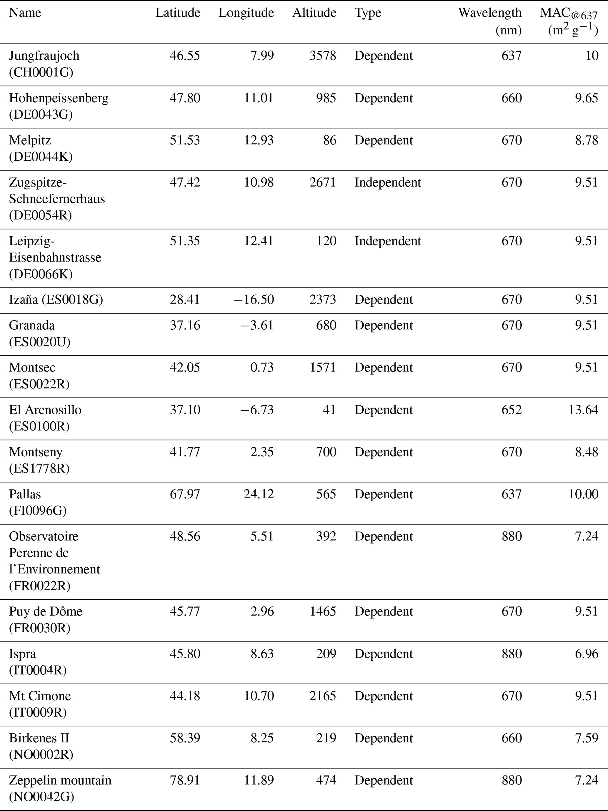
All absorption measurements within ACTRIS and EMEP are taken using a variety of filter-based photometers: Multi-Angle Absorption Photometer (MAAP), Particle Soot Absorption Photometer (PSAP) Continuous Light Absorption Photometer (CLAP) and the Aethalometer (AE-31). Information on instrument type at the various sites is included in Table 1, and procedures for harmonization of measurement protocols to produce comparable datasets are described in Laj et al. (2020) in detail. Zanatta et al. (2016) suggested that a mass absorption cross-section (MAC) value of 10 m² g⁻¹ (geometric standard deviation of 1.33) at a wavelength of 637 nm can be considered to be representative of the mixed boundary layer at European ACTRIS background sites, where BC is expected to be internally mixed to a large extent. Assuming an absorption Ångström exponent (AAE) is equal to unity, i.e. assuming no change in MAC for different sources (Zotter et al., 2017), we extrapolated the MACs at 637 nm (MAC_@λ1) to the measurement wavelengths of our study (MAC_@λ2) using the following equation:

$$\begin{array}{}\text{(1)}& \begin{array}{rl}{\mathrm{MAC}}_{\mathrm{@}\mathit{\lambda }\mathrm{2}}& ={\mathrm{MAC}}_{\mathrm{@}\mathit{\lambda }\mathrm{1}}({\displaystyle \frac{\mathit{\lambda }\mathrm{1}}{\mathit{\lambda }\mathrm{2}}}{)}^{\mathrm{AAE}}\\ & \stackrel{\text{yields}}{⟶}{\mathrm{MAC}}_{\mathrm{@}\mathit{\lambda }\mathrm{2}}=\mathrm{10}({\displaystyle \frac{\mathrm{637}}{\mathit{\lambda }\mathrm{2}}}{)}^{\mathrm{1}},\end{array}\end{array}$$

following Lack and Langridge (2013). The resulting MAC values for each measurement station are shown in Table 1.

Table 1 Observation sites from the ACTRIS platform used to perform the inversions (dependent observations) and to validate the posterior emissions (independent observations) (the altitude indicates the sampling height in metres above sea level). A Multi-Angle Absorption Photometer (MAAP) was used at all sites, except El Arenosillo (ES0100R), where a Continuous Light Absorption Photometer (CLAP) was used, Birkenes (NO0002R), where a Particle Soot Absorption Photometer (PSAP) was used and Observatoire Perenne de l'Environnement (FR0022R) and Zeppelin (NO0042G), where an Aethalometer (AW-31) was used.

2.2 Source–receptor matrix (SRM) calculations

SRMs for each of the 17 receptor sites (Table 1) were calculated using the Lagrangian particle dispersion model FLEXPART version 10.4 (Pisso et al., 2019). The model releases computational particles that are tracked backward in time based on 3-hourly operational meteorological analyses from the European Centre for Medium-Range Weather Forecasts (ECMWF) with 137 vertical layers and a horizontal resolution of 1^∘ × 1^∘. The tracking of BC particles includes gravitational settling for spherical particles, with an aerosol mean diameter of 0.25 µm, a logarithmic standard deviation of 0.3 and a particle density of 1500 kg m⁻³ (Long et al., 2013). FLEXPART also simulates dry and wet deposition (Grythe et al., 2017), turbulence (Cassiani et al., 2014) and unresolved mesoscale motions (Stohl et al., 2005) and includes a deep convection scheme (Forster et al., 2007). SRMs were calculated for 30 d backward in time, at temporal intervals that matched measurements at each receptor site. This backward tracking is sufficiently long to include almost all BC sources that contribute to surface concentrations at the receptors given a typical atmospheric lifetime of 3–11 d (Bond et al., 2013).

2.3 Bayesian inverse modelling

The Bayesian inversion framework FLEXINVERT+ described in detail in Thompson and Stohl (2014) was used to optimize emissions of BC before (January to mid-March 2020) and during the COVID-19 lockdown period in Europe (mid-March to end of April 2020). To show potential differences in the signal from the 2020 restrictions, emissions were optimized with the same setup during the same period (January to April) in the previous 5 years (2015–2019). Note that the number of stations in the inversions of 2015–2019 was slightly higher (20 stations against 15 that were used in 2020), due to different data availability. The algorithm finds the optimal emissions which lead to FLEXPART-modelled concentrations that better match the observations considering the uncertainties for observations, prior emissions and SRMs. Specifically, the state vector of BC concentrations, $y_{(M\times \mathrm{1})}^{\mathrm{mod}}$, at M points in space and time can be modelled given an estimate of the emissions, x_(N×1), of the N state variables discretized in space and time, while atmospheric transport and deposition are linear operations described by the Jacobian matrix of SRMs, H_(M×N):

$$\begin{array}{}\text{(2)}& y^{\mathrm{mod}}=Hx+\mathit{ϵ},\end{array}$$

where ϵ is an error associated with model representation, such as the modelled transport and deposition or the measurements. Since H is not invertible or may not have a unique inverse, according to Bayesian statistics, the inverse problem can be described as the maximization of the probability density function of the emissions given the prior information and observations. This is equivalent to the minimum of the cost function:

$$\begin{array}{}\text{(3)}& \begin{array}{rl}\mathbf{J}\left(\mathit{x}\right)& ={\displaystyle \frac{\mathbf{1}}{\mathbf{2}}}{\left(\mathit{x}-{\mathit{x}}_{\mathit{b}}\right)}^{\mathit{T}}{\mathbf{B}}^{-\mathbf{1}}\left(\mathit{x}-{\mathit{x}}_{\mathit{b}}\right)\\ & +{\displaystyle \frac{\mathbf{1}}{\mathbf{2}}}{\left(\mathit{y}-\mathbf{H}\mathit{x}\right)}^{\mathit{T}}{\mathbf{R}}^{-\mathbf{1}}(\mathit{y}-\mathbf{H}\mathit{x}),\end{array}\end{array}$$

where y is the vector of observed BC concentrations, and x and x_b are the vectors of optimized and prior emissions, respectively, while B and R are the error covariance matrices that weight the posterior–prior flux and observation–model mismatches, respectively. Based on Bayes' theorem, the most probable posterior emissions, x, are given by the following equation (Tarantola, 2005):

$$\begin{array}{}\text{(4)}& \mathit{x}={\mathit{x}}_{\mathit{b}}+{\mathbf{BH}}^{\mathbf{T}}{\left({\mathbf{HBH}}^{\mathbf{T}}+\mathbf{R}\right)}^{-\mathbf{1}}(\mathit{y}-\mathbf{H}{\mathit{x}}_{\mathit{b}}).\end{array}$$

Here, posterior emissions were calculated weekly between 1 January and 30 April 2020. The aggregated inversion grid (25–75^∘ N and 10^∘ W–50^∘ E) and the average SRM for inversions are shown in Fig. 1, while the measurement stations are listed in Table 1. The variable grid uses high resolution in regions in which there are many stations and hence strong contribution from emissions, while it lowers resolution in regions that lack measurement stations, following a method proposed by Stohl et al. (2010).

Figure 1 Aggregated inversion grid used for the (a) 2015–2019 and (b) 2020 inversions, respectively. The dependent measurements that were used in the inversion were taken from stations highlighted in red. The two independent stations that were used for the validation are shown in blue. (c, d) Footprint emission sensitivity (i.e. SRM) averaged over all observations and time steps for each of the inversions. Red points denote the location of each measurement site.

Prior emission errors B are correlated in space and time, but very little is known about the true temporal and spatial error correlation patterns. The spatial error correlation for the emissions is defined as an exponential decay over distance (we assume that emissions on land and ocean are not correlated). The temporal error correlation matrix is described similarly using the time difference between grid cells in different time steps. The full temporal and spatial correlation matrix is given by the Kronecker product (see Thompson and Stohl, 2014). The error covariance matrix for the emissions is the matrix product of correlation pattern and the error covariance of the prior fluxes. We calculate the error on the emissions in each grid cell (on the fine grid) as a fraction of the maximum value out of that grid cell and the eight surrounding ones.

The observation error covariance matrix R combines measurement, transport model and representation errors. For the measurement errors, we use values given by the data providers. Transport model errors are difficult to quantify and depend not only on the model but also on the meteorological inputs. Therefore, we do not quantify the full transport error but only the part of it that can be estimated from FLEXPART, i.e. the stochastic uncertainty (see Stohl et al., 2005). As regards to representation errors, we consider observation representation error and model aggregation error. The observation representation error is calculated from the standard deviation of all measurements available in a user-specified measurement averaging time interval, based on the idea that if the measurements are fluctuating strongly within that interval, then their mean value is associated with higher uncertainty than if the measurements are steady (Bergamaschi et al., 2010). The aggregation error is attributed to reduction of the spatial resolution of the model and is calculated by projecting the loss of information in the state space into the observation space (Kaminski et al., 2001). Hence, the observation error covariance matrix is defined as the diagonal matrix with elements equal to the quadratic sum of the measurement, transport model and measurement representation errors (Thompson and Stohl, 2014).

Theoretically, the algorithm can calculate negative posterior emissions, which are physically unlikely. To tackle this problem, an inequality constraint was applied on the emissions following the method of Thacker (2007) that applies the constraint as “error-free” observations:

$$\begin{array}{}\text{(5)}& \widehat{\mathit{x}}=\mathit{x}+{\mathbf{AP}}^{\mathbf{T}}{\left({\mathbf{PAP}}^{\mathbf{T}}\right)}^{-\mathbf{1}}(\mathit{c}-\mathbf{P}\mathit{x}),\end{array}$$

where A is the posterior error covariance matrix, P is a matrix operator to select the variables that violate the inequality constraint and c is a vector of the inequality constraint, which in this case is zero.

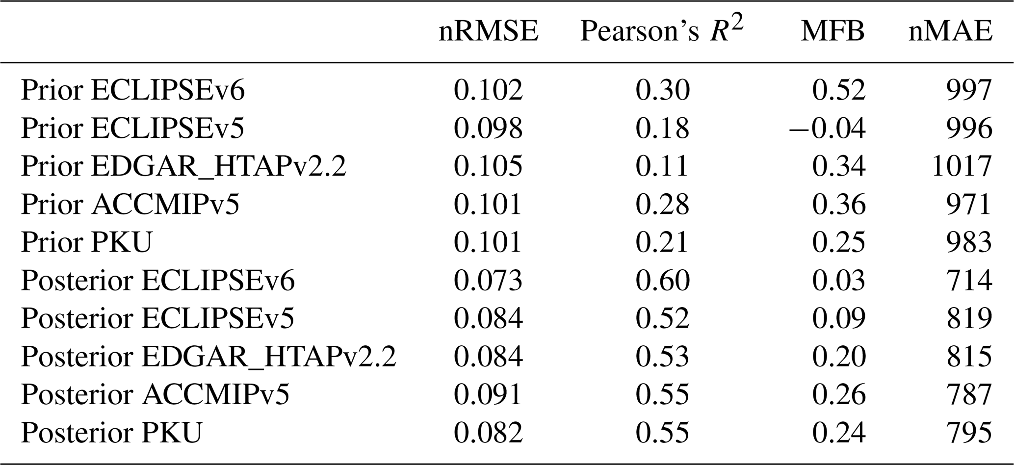
We evaluated the assumptions made on the error covariance matrices for the prior emissions and the observations using the reduced χ² statistics (B and R). When χ² is equal to unity, the posterior solution is within the limits of the prescribed uncertainties. The latter is the value of the cost function at the optimum (Thompson et al., 2015). In the inversions performed here, the calculated χ² values were between 0.8 and 1.5, indicating that the chosen uncertainty parameters are close to the ideal ones. The number of measurements used in each inversion was equal to 12 538 from 17 stations. To select the inversion that provides the most statistically significant result, an evaluation of the improvement in the posterior modelled concentrations, with respect to the prior ones, against the observations was performed (Fig. 2). The resulting values of each of the statistical measures that were performed are given in detail in Table 2. Note that this is not a validation of the posterior emissions because the comparison is only done for the observations that were included in the inversion (dependent observations), and the inversion algorithm has been designed to reduce the model–observation mismatches. This means that the reduction of the posterior concentration mismatches to the observations is determined by the weighting that is given to the observations with respect to the prior emissions. A proper validation of the posterior emissions is performed against observations that were not included in the inversion (independent observations) in Sect. 3.3.

Figure 2 Scatter plots of prior and posterior concentrations against dependent observations (observations that were included in the inversion framework) from ACTRIS from January to April 2020. Four statistical measures (nRMSE, Pearson's R², MFB and nMAE) were used to assess the performance of each inversion using five different prior emission inventories for BC (ECLIPSEv5, v6, ACCMIPv5, EDGAR_HTAPv2.2 and PKU).

Table 2 Statistical measures (RMSE, Pearson's R², MFB and nMAE) for each of the prior and posterior concentrations against dependent observations (observations that were used in the inversion algorithm) for BC (eBC). Note that the inversion using ECLIPSEv6 prior emission dataset gave the best agreement with the observations, and therefore the results of this inversion are presented here.

2.4 Prior emissions

As a priori emissions in the inversions, the ECLIPSE version 5 and 6 (Evaluating the CLimate and Air Quality ImPacts of ShortlivEd Pollutants) (Klimont et al., 2017), EDGAR (Emissions Database for Global Atmospheric Research) version HTAP_v2.2 (Janssens-Maenhout et al., 2015), ACCMIP (Emissions for Atmospheric Chemistry and Climate Model Intercomparison Project) version 5 (Lamarque et al., 2013) and PKU (Peking University) (Wang et al., 2014b) were used (Fig. 3). All inventories include the basic emission sectors (e.g. waste burning, industrial combustion and processing, all means of transportation (aerial, surface, ocean), energy conversion and residential and commercial combustion; see references therein). Biomass burning emissions were adopted from the Global Fire Emissions Database, Version 4.1s (GFEDv4.1s) (Giglio et al., 2013). Note that the a priori emissions used in the inversions of 2015–2019 period corresponded to year 2015 of ECLIPSEv6, and they were not interpolated for the years between 2015 and 2020, for which the ECLIPSEv6 emissions were calculated. We calculate that the anthropogenic emissions of BC in Europe between January–April 2015 and January–April 2020 in ECLIPSEv6 differ by 3.4 % only, and therefore we expected that this would not add significant bias in our calculations.

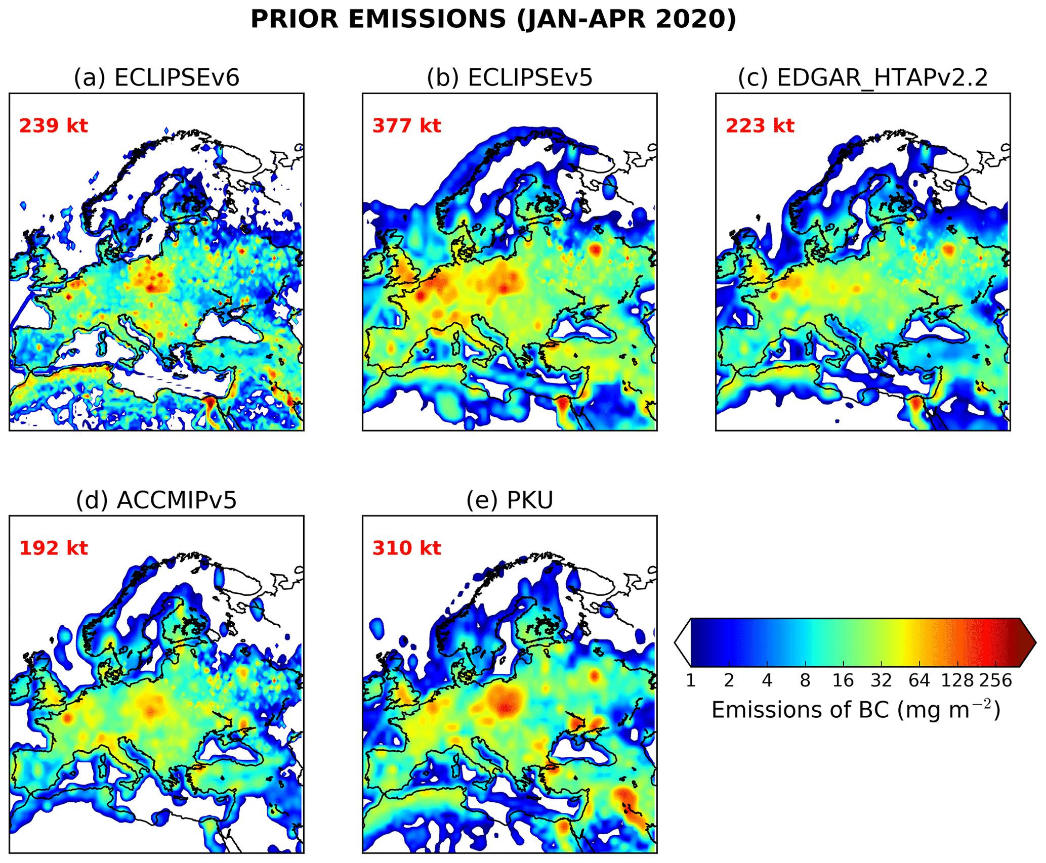
Figure 3 Prior emissions of black carbon (BC) used in the inversions. BC emissions from anthropogenic sources were adopted from ECLIPSE version 5 and 6 (Evaluating the CLimate and Air Quality ImPacts of ShortlivEd Pollutants) (Klimont et al., 2017), EDGAR (Emissions Database for Global Atmospheric Research) version HTAP_v2.2 (Janssens-Maenhout et al., 2015), ACCMIP (Emissions for Atmospheric Chemistry and Climate Model Intercomparison Project) version 5 (Lamarque et al., 2013) and PKU (Peking University) (Wang et al., 2014b). Biomass burning emissions of BC from Global Fire Emissions Database (GFED) version 4.1 (Giglio et al., 2013) were added to each of the aforementioned inventories.

2.5 MERRA-2 (Modern-Era Retrospective Analysis for Research and Applications Version 2)

The MERRA-2 reanalysis dataset for BC (Randles et al., 2017) assimilates bias-corrected aerosol optical depth (AOD) from Moderate Resolution Imaging Spectroradiometer (MODIS), Advanced Very High Resolution Radiometer (AVHRR) instruments, Multiangle Imaging SpectroRadiometer (MISR) and Aerosol Robotic Network (AERONET) with the Goddard Earth Observing System Model Version 5 (GEOS-5). BC and other aerosols in MERRA-2 are simulated with the Goddard Chemistry, Aerosol, Radiation and Transport (GOCART) model and delivered in hourly to monthly temporal resolution and at 0.5^∘ × 0.625^∘ spatial resolution. The product has been validated for AOD, PM and BC extensively (Buchard et al., 2017; Qin et al., 2019; Randles et al., 2017; Sun et al., 2019). The Ångström exponent (AE), a measure of how the AOD changes relative to the various wavelength of light, is derived here from AOD469, AOD550, AOD670 and AOD865, by fitting the data to the linear transform of Ångström's empirical expression:

$$\begin{array}{}\text{(6)}& {\mathit{\tau }}_{\mathit{\lambda }}={\mathit{\tau }}_{{\mathit{\lambda }}_{\mathrm{0}}}({\displaystyle \frac{\mathit{\lambda }}{{\mathit{\lambda }}_{\mathrm{0}}}}{)}^{-a},\end{array}$$

where τ_λ is the known AOD at wavelength λ (in nm), ${\mathit{\tau }}_{{\mathit{\lambda }}_{\mathrm{0}}}$ is the AOD at 1000 nm and α stands for AE (Gueymard and Yang, 2020).

2.6 Absorption Ångström exponent from Aerosol Robotic Network (AERONET) data

Aerosol composition over Europe during the COVID-19 lockdown was confirmed using the AERONET data (Holben et al., 1998). AERONET provides globally distributed observations of spectral aerosol optical depth (AOD), inversion products and precipitable water in diverse aerosol regimes. The AE for a spectral dependence of 440–870 nm is related to the aerosol particle size. Values less than 1 suggest an optical dominance of coarse particles corresponding to dust, ash and sea spray aerosols, while values greater than 1 imply dominance of fine particles such as smoke and industrial pollution (Eck et al., 1999). We chose data from five stations covering Western, central and Eastern Europe, for which cloud-free measurements exist for the lockdown period, namely Ben Salem (9.91^∘ E, 35.55^∘ N), Minsk (27.60^∘ E, 53.92^∘ N), Montsec (0.73^∘ E, 42.05^∘ N), MetObs Lindenberg (14.12^∘ E, 52.21^∘ N) and Munich University (11.57^∘ E, 48.15^∘ N). We used Level 1.5 absorption AE (AAE) measurements for the COVID-19 lockdown period (14 March to 30 April 2020).

2.7 Statistical measures

For the performance evaluation of the inversion results against dependent (observations that were included in the inversion) and independent observations (observations that were not included in the inversion), four different statistical quantities were used.

1. Pearson's correlation coefficient was calculated as follows:

   $$\begin{array}{}\text{(7)}& R_{\mathrm{mo}}={\displaystyle \frac{n{\sum }_{i=\mathrm{1}}^n{m}_i{o}_i-{\sum }_{i=\mathrm{1}}^n{m}_i{\sum }_{i=\mathrm{1}}^n{o}_i}{\sqrt{n{\sum }_{i=\mathrm{1}}^n{m}_i^{\mathrm{2}}-({\sum }_{i=\mathrm{1}}^n{m}_i{)}^{\mathrm{2}}}\sqrt{n{\sum }_{i=\mathrm{1}}^n{o}_i^{\mathrm{2}}-({\sum }_{i=\mathrm{1}}^n{o}_i{)}^{\mathrm{2}}}}},\end{array}$$

   where n is the sample size, m and o the individual sample points for model concentrations and observations indexed with i.

2. The normalized root mean square error (nRMSE) was calculated as follows:

   $$\begin{array}{}\text{(8)}& \mathrm{nRMSE}={\displaystyle \frac{\sqrt{{\sum }_{i=\mathrm{1}}^n\frac{\mathrm{1}}{n}(m_i-o_i{)}^{\mathrm{2}}}}{o_i^{\max }-o_i^{\min }}}.\end{array}$$

3. The mean fractional bias (MFB) was selected as a symmetric performance indicator that gives equal weights to under- or overestimated concentrations (minimum to maximum values range from −200 % to 200 %) and is defined as

   $$\begin{array}{}\text{(9)}& \mathrm{MFB}={\displaystyle \frac{\mathrm{1}}{n}}{\displaystyle \frac{{\sum }_{i=\mathrm{1}}^n\left(m_i-o_i\right)}{{\sum }_{i=\mathrm{1}}^n\left(\frac{m_i+o_i}{\mathrm{2}}\right)}}.\end{array}$$

4. The mean absolute error was computed normalized (nMAE) over the average of all the actual values (observations here), which is a widely used simple measure of error:

   $$\begin{array}{}\text{(10)}& \mathrm{nMAE}={\displaystyle \frac{{\sum }_{i=\mathrm{1}}^n\left|m_i-o_i\right|}{{\sum }_{i=\mathrm{1}}^n{o}_i}}.\end{array}$$

2.8 Region definitions

All country and regional masks are publicly available. Regions used for statistical processing purposes were adopted from the United Nations Statistics Division (https://unstats.un.org/home/, last access: 25 September 2020). Accordingly, Northern Europe includes UK, Norway, Denmark, Sweden, Finland, Iceland, Estonia, Latvia and Lithuania. Southern Europe includes Spain, Italy, Greece, Slovenia, Croatia, Bosnia, Serbia, Albania and North Macedonia. Western Europe is defined by France, Belgium, Holland, Germany, Austria and Switzerland. Eastern Europe includes Poland, Czechia, Slovakia, Hungary, Romania, Bulgaria, Moldova, Ukraine, Belarus and Russia.

3 Results

3.1 Optimized (posterior) emissions from Bayesian inversion

We performed five inversions for BC over Europe for 1 January–30 April 2020, each with different prior emissions from ECLIPSE version 5 and 6, EDGAR version HTAP_v2.2, ACCMIP version 5 and PKU (Fig. 3). Total prior emissions of BC in Europe from the five emission inventories for the period of the inversion ranged between 192–377 kt. We evaluated the assumptions made on the error covariance matrices for the prior emissions and the observations using the reduced χ² statistic (B and R; see Sect. 2.3). When χ² is equal to unity, the posterior solution is within the limits of the prescribed uncertainties. The performance of the inversions with the five different prior inventories was evaluated using four statistical parameters (see Sect. 2.7). The best performance of the inversions was achieved using ECLIPSEv6 (Table 2 and Fig. 2) with the smallest nRMSE (0.073) value, the largest Pearson's R² (0.60), the MFB value closest to zero (0.03) and the smallest nMAE (714). Therefore, all the results presented below correspond to this inversion.

Posterior emissions of BC were calculated to be 191 kt in the inversion domain (10^∘ W–50^∘ E, 25–75^∘ N) or approximately 20 % smaller than those in ECLIPSEv6 (239 kt) (Fig. 4). Note that these numbers refer to the whole inversion domain (not only Europe) and the whole study period (January–April 2020). The largest posterior differences were found in the eastern part of the domain (20–50^∘ E, 45–55^∘ N), where emissions dropped from 35 to 29 kt. Emissions of BC in the western part of the inversion domain (10^∘ W–20^∘ E, 45–55^∘ N) declined by almost 11 % (from 45 to 40 kt) compared to those in the north part (5^∘ W–35^∘ E, 55–70^∘ N) that covers Scandinavian countries (from 8.7 to 6.4 kt). Finally, in the southern part (10^∘ W–50^∘ E, 35–45^∘ N) of the domain (Spain, Italy, Greece), the posterior emissions also decreased by 21 % relative to the priors (from 61 to 48 kt). The largest country decreases were seen in France (from 14 to 8.2 kt), Italy (from 8.0 to 5.9 kt), UK (from 4.4 to 3.1 kt) and Germany (from 4.5 to 4.1 kt). Surprisingly, BC emissions were slightly enhanced in Poland (from 21 to 23 kt) and in Spain (from 6.3 to 7.5 kt). In general, inversion algorithms reduce the mismatches between modelled concentrations and observations by correcting emissions (Sect. 2.3). If decreased posterior emissions are calculated during the whole inversion period (before and during the lockdowns), impact from the COVID-19 restrictions cannot be concluded, and, most likely, the reduced emissions are due to errors in the prior emissions. In the next section (Sect. 3.2), we demonstrate that this decrease was due to the COVID-19 lockdowns, by comparing posterior emissions with emissions from previous years, as well as with the respective emissions before and during the lockdown measures.

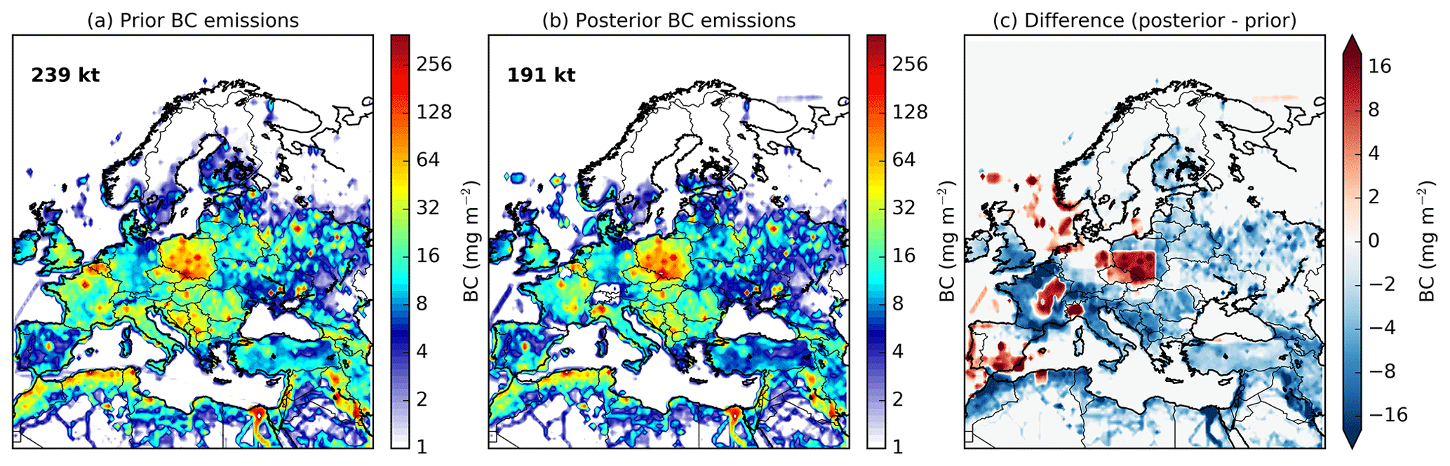
Figure 4 (a) Prior emissions of BC from ECLIPSEv6, (b) optimized (posterior) BC emissions after processing the ACTRIS data into the inversion algorithm and (c) difference between posterior and prior emissions. All the results correspond to the inversion yielding the best results (Table 2 and Fig. 2).

3.2 Comparison with previous years

We also performed inversions for 2015–2019 for the same period as the 2020 lockdowns (January–April) using almost the same measurement stations and keeping the same settings. The difference in BC emissions during the lockdown in 2020 (14 March to 30 April) to the respective emissions during the same period in 2015–2019 (14 March to 30 April) is shown in Fig. 5a (emission anomaly), together with the gross domestic product (GDP) (Kummu et al., 2020) in 5b and temperature anomaly from ERA-5 (Copernicus Climate Change Service (C3S), 2020) in 5c for the same period as the emission anomaly. The difference in the 2020 emissions of BC during the lockdown from the respective emissions in the same period in each of the previous years (2015–2019) is illustrated in Fig. S1. As an independent source of information, active fires from the MODIS satellite product MCD14DL (Giglio et al., 2003) are also shown in Fig. 5a and Fig. S1.

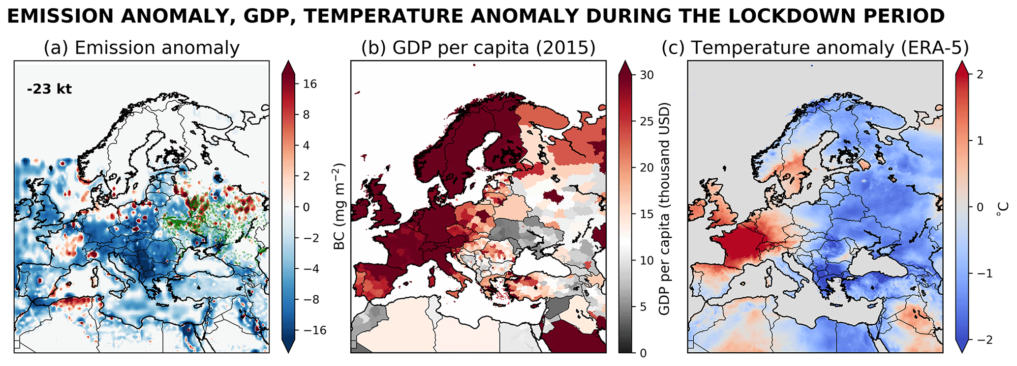
Figure 5 (a) Difference in posterior BC emissions during the lockdown (14 March to 30 April 2020) in Europe from the respective emissions during the same period in 2015–2019, (b) GDP from Kummu et al. (2020) and (c) temperature anomaly from ERA-5 (Copernicus Climate Change Service (C3S), 2020) for the same period as the emission anomaly. The base GDP value below which a low income can be assumed was set to USD 12 000. Active fires from MODIS are plotted together with the emission anomaly (green dots).

Overall, BC emissions decreased by ∼46 kt during the COVID-19 lockdown in the inversion domain (10^∘ W–50^∘ E, 25–70^∘ N) as compared with the same period in the previous 5 years. We record a significant decrease in BC emissions in central Europe (northern Italy, Austria, Germany, Spain and some Balkan countries) (Fig. 5). On average, emissions were 23 kt lower (63 to 40 kt) over Europe during the lockdown in 2020 than in the same period of 2015–2019 (Fig. 5). The decrease has the same characteristics when compared to each of previous years since 2015 (Fig. S1) based on measurements of BC in similar regions to those used for the 2020 inversion. The countries that showed drastic reductions in BC emissions during the lockdowns were those that suffered from the pandemic dramatically, with many human losses, strict social distancing rules and consequently less transport. Specifically, compared with the previous 5 years, the 2020 emissions of BC during the lockdowns dropped by 20 % in Italy (3.4 to 2.7 kt), 40 % in Germany (3.3 to 2.0 kt), 34 % in Spain (4.7 to 3.1 kt) and 22 % in France (3.5 to 2.7 kt) and remained the same or were slightly enhanced in Poland (∼9.2 kt) and Scandinavia (∼1.2 kt). Air quality in Poland may not be Europe's worst, but its emissions stand out for their large spatial spread. Poland's air pollution stems from its use of cheap coal for home heating rather than cleaner natural gas common in neighbouring countries. This causes smoke particles to rise up to 3 times higher than European average levels in winter and early spring (Bertelsen and Mathiesen, 2020). Overall, BC emissions during the 2020 lockdowns in Western Europe declined by 32 % (8.8 to 6.0 kt), in Southern Europe by 42 % (17 to 9.9 kt) and in Northern Europe by 29 % (5.4 to 3.8 kt) as compared to the 2015–2019 period. BC emissions in Eastern Europe were slightly increased during the 2020 lockdown as compared to the same period in the last 5 years (28 to 31 kt). The hotspot emissions in Eastern Europe coincide with the presence of active fires as revealed from MODIS (Fig. 5a). Note that these numbers correspond to BC emissions during the COVID-19 lockdown period only (mid-March–April 2020).

Some localized areas of increased BC emissions exist in southern France, Belgium, northern Germany and Eastern Europe (Fig. 5), which are observed relative to almost every year since 2015 (Fig. S1). While some hotspots in France cannot be easily explained, increased emissions in Eastern European countries are likely due to increased residential combustion, as people had to stay at home during the lockdown. The combination of the financial consequences of the COVID-19 lockdown with the relatively low GDP per capita in these countries and the fact that from mid-March to end of April 2020 surface temperatures in these countries were significantly lower than in previous years is suggestive of increased emissions due to residential combustion. This source is most important in Eastern Europe (Klimont et al., 2017). Although residential combustion can be performed for heating or cooking needs in poorer countries, it is also believed to provide a more natural type of warmth and a comfortable and relaxing environment. Hence, it should not be assumed as an emission source in countries with lower GDPs only, especially as people spent more time at home. Moreover, the prevailing average temperatures over Europe during the lockdown were below 15 ^∘C (Fig. S2), a temperature used as a basis temperature below which residential combustion increases (Quayle and Diaz, 1980; Stohl et al., 2013).

3.3 Uncertainty and validation of the posterior emissions

One of the basic problems when dealing with inverse modelling is that changing model, observational or prior uncertainties can have drastic impacts on posterior emissions. We addressed this issue by finding the optimal parameters, in order to have a reduced χ² statistic around unity (see Sect. 2.3). However, there are two other sources of uncertainty that, although not linked with the inversion algorithm, could affect posterior emissions drastically. The first is the use of different prior emissions; to estimate this type of uncertainty, we performed five inversions for January to April 2020 using each of the prior emission datasets (ECLIPSEv6 and v5, EDGAR_HTAPv2.2, ACCMIPv5 and PKU). The uncertainty was calculated as the gridded standard deviation of the posterior emissions resulting from the five inversions. The second type of uncertainty concerns measurement of BC, which is defined as a function of five properties (Petzold et al., 2013). However, as of today, no single instrument exists that can measure all of these properties at the same time. Hence, BC is not a single particle constituent, rather an operational definition depending on the measurement technique (Petzold et al., 2013). Here we use light absorption coefficients (Petzold et al., 2013) converted to equivalent BC (eBC) using the mass absorption cross-section (MAC). The MAC is instrument-specific and wavelength-dependent. The site-specific MAC values used to convert the filter-based light absorption to eBC can be seen in Table 1. It has been reported that MAC values vary from 2–3 up to 20 m² g⁻¹ (Bond and Bergstrom, 2006). To estimate the uncertainty of the posterior fluxes associated with the variable MAC, we performed a sensitivity study for January to April 2020 using MAC values of 5, 10 and 20 m² g⁻¹ at all stations, as well as variable MAC values for each station (Table 1). Since these values are log-normally distributed, the uncertainty is calculated as the geometric standard deviation. The impact of other sources of uncertainty, such as those referring to scavenging coefficients, particle size and density that are used in the model has been studied before and is significantly smaller than that of the sources of uncertainty that are considered here (Evangeliou et al., 2018; Grythe et al., 2017).

The posterior emissions are less sensitive to the use of different MACs than the use of different prior inventories (Fig. 6). The relative uncertainty due to different use of MAC values was up to 20 %–30 % in most of Europe and increases dramatically (∼100 %) far from the observations. The emission uncertainty of BC from the use of different priors was estimated to be up to 40 % in Europe and shows very similar characteristics (same hotspot regions and larger values where measurements are lacking). Overall, the combined uncertainty of BC emissions was ∼60 % in Europe.

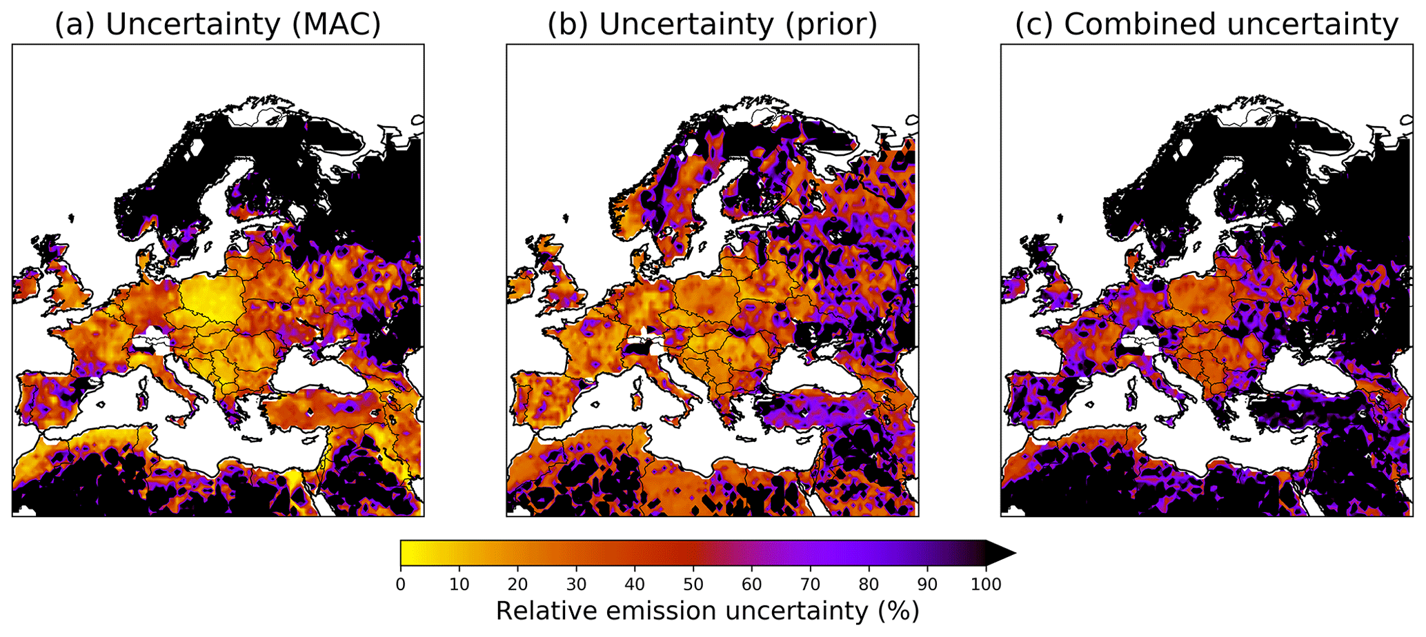
Figure 6 (a) Uncertainty of BC emissions due to the use of variable MAC values to convert from aerosol absorption to eBC concentrations that are used by the inversion algorithm. (b) Uncertainty due to the use of five different prior emissions inventories for BC. (c) Combined uncertainty.

Validation of top-down emissions obtained by inversion algorithms can be proper only if measurements that were not included in the inversion are to be used (independent observations). For this reason, we left observations from two stations (DE0054K and DE0066R; Table 1) out of the inversion. Due to the higher measurement station density in central Europe, we randomly selected two German stations, rather than from a country that is adjacent to regions that lack observations.

The prior, optimized and measured concentrations are shown in Fig. 7, together with MERRA-2 surface BC concentrations at the same stations. The average footprint emission sensitivities are also given for the period of the lockdown. At station DE0054K, prior emissions represent observations very well until the beginning of the lockdown and then fail (Fig. 7). On the other hand, the posterior emissions represent the variant concentrations during the lockdown effectively and also manage to capture some concentration peaks, which is reflected by a lower nRMSE. Backward modelling showed that the enhanced concentrations originate from northern Germany and the Netherlands, where posterior emissions were increased compared with the prior ones (Fig. 4). A similar pattern was seen at station DE0066K, although this station showed concentrations of up to 4 mg m⁻³ (Fig. 7). Again, the optimized emissions managed to represent the peaks at the end of January 2020 and at the beginning of the lockdown, which is again reflected by nRMSE values reduced by a factor of 2 and MFB close to zero as compared to the priors. The larger concentrations during the lockdown result from increased emissions over eastern Germany, Poland and the Netherlands, as well as from oil industries in the North Sea (Fig. 4b). In all these regions, the footprint emissions' sensitivities corresponding to the two independent stations were the highest.

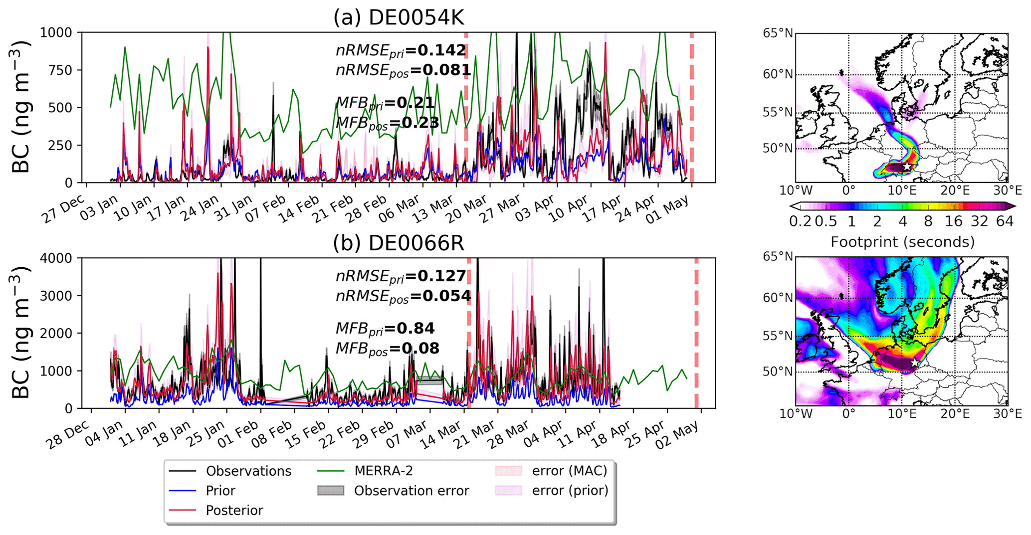
Figure 7 Prior and posterior BC concentrations at (a) DE0054K and (b) DE0066R stations that were not included in the inversion are compared with observations. The validation is done by calculating the nRMSEs and MFBs for the prior and posterior concentrations. The uncertainty of the observations is also given, together with the posterior uncertainties in the concentrations calculated from the use of different MAC and prior emissions. For comparison, we plot the concentrations from MERRA-2 at the same two stations. The vertical dashed lines denote the period of the lockdown in most of Europe. In the right-hand panels of (a) and (b), the average footprint emission sensitivities are given at each independent station for the period of the lockdown.

4 Discussion

The improved air quality that Europe experienced during the lockdown was also evident from the assimilated MERRA-2 satellite-based BC data. The latter are plotted in Fig. S3 (left axis) for 2015–2020, together with the posterior emissions calculated in the present study (right axis). For instance, weekly average concentrations of BC over Europe in MERRA-2 (Fig. S3, bottom). Many of the ACTRIS stations reported increased light absorption at the beginning of the lockdown (e.g. Fig. 7); MERRA-2 data show the same patterns in France, Italy, UK and Spain and in all of Europe, in general. This can be explained by residential combustion, considering that the surface temperature during the lockdown was lower than in previous years (Fig. 5). The latter was confirmed by the MERRA-2 reanalysis Ångström exponent (AE) parameter at 470–870 nm, which shows higher values over central and Eastern Europe during the lockdown in 2020 than in the same period of the previous years (Fig. 8a, b). Larger AE values confirm the presence of wood-burning aerosols (Eck et al., 1999). The fact that during the COVID-19 lockdown, residential combustion was a significant aerosol source in Europe, as compared to the previous years, was also confirmed by real-time observations of absorption AE from the AERONET data at five selected stations over Europe (Fig. 8c). Measured absorption AE was higher during mid-March to April 2020 than in the same period of the last 5 years.

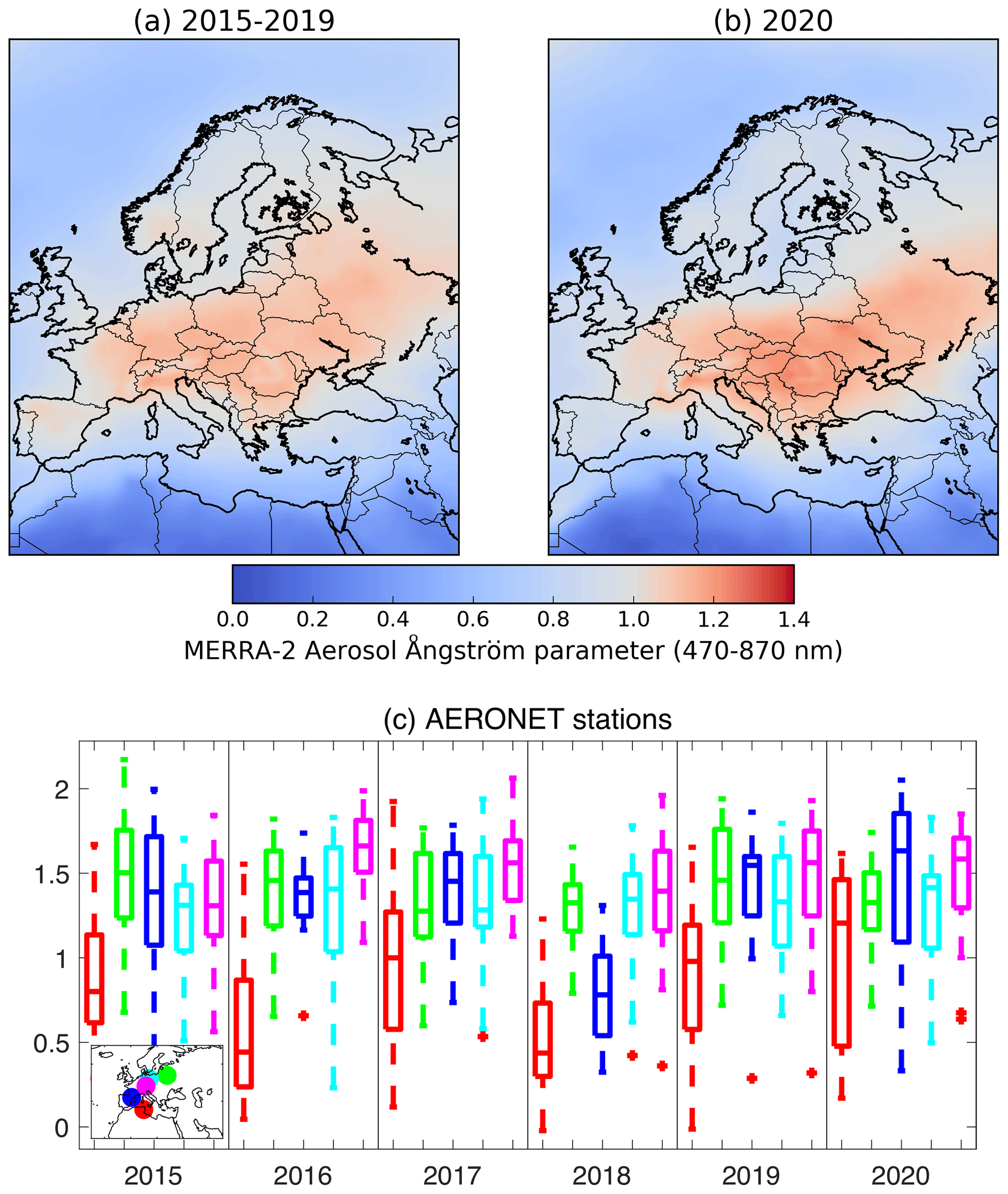
Figure 8 (a) Average total aerosol Ångström parameter (470–870 nm) over Europe (mid-March to April) in the 5 previous years (2015–2019) and (b) in 2020 (lockdown). (c) AERONET Absorption AE in Ben Salem (9.91^∘ E, 35.55^∘ N; in red), Minsk (27.60^∘ E, 53.92^∘ N; green), Montsec (0.73^∘ E, 42.05^∘ N; blue), MetObs Lindenberg (14.12^∘ E, 52.21^∘ N; magenta) and Munich University (11.57^∘ E, 48.15^∘ N) during mid-March to April in all years since 2015.

Emissions of BC calculated with Bayesian inversion for the lockdown period dropped substantially in most of the countries that suffered from further spread of the virus and, accordingly, from strict lockdown measures, as compared to the respective emissions before the lockdowns (Fig. S3). Specifically, the decrease in France was as high as 42 %, 8 % in Italy, 21 % in Germany, 11 % in Spain and 13 % in the UK. Emissions also declined in Scandinavia by 5 %, although Sweden did not enforce a lockdown. Overall, a reduction in BC emissions of about 11 % can be concluded for Europe as a whole due to the lockdown. Stronger decreases in Eastern Europe were likely partly compensated for by increased residential combustion, resulting from the prevailing low temperatures.

We report a 23 kt decrease in BC emissions in Europe during the lockdown that partially resulted from the COVID-19 outbreak, as compared to the same period in all previous years since 2015, based on particle light absorption measurements. We highlight these changes in BC emissions partially as a result of COVID-19 restrictions by plotting the temporal variability of the BC emissions in the 5 previous years (2015–2019) for France, Italy, Germany, Spain, Scandinavia and Europe (Fig. 9). We record decreases in BC emissions in France, Italy, Germany and Scandinavia in mid-March to April 2020, opposite to what was estimated for all years between 2015 and 2019, which is obviously due to COVID-19. The UK and Spain showed a similar decrease in mid-March to April 2020 emissions as in all previous years (2015–2019). However, the estimated posterior BC emissions during the 2020 lockdowns were significantly lower than those of the same period in any of the previous years. Overall, emissions declined by 20 % in Italy, 40 % in Germany, 34 % in Spain and 22 % in France and remained the same and slightly enhanced in Scandinavia and Poland as compared to those of the last 5 years.

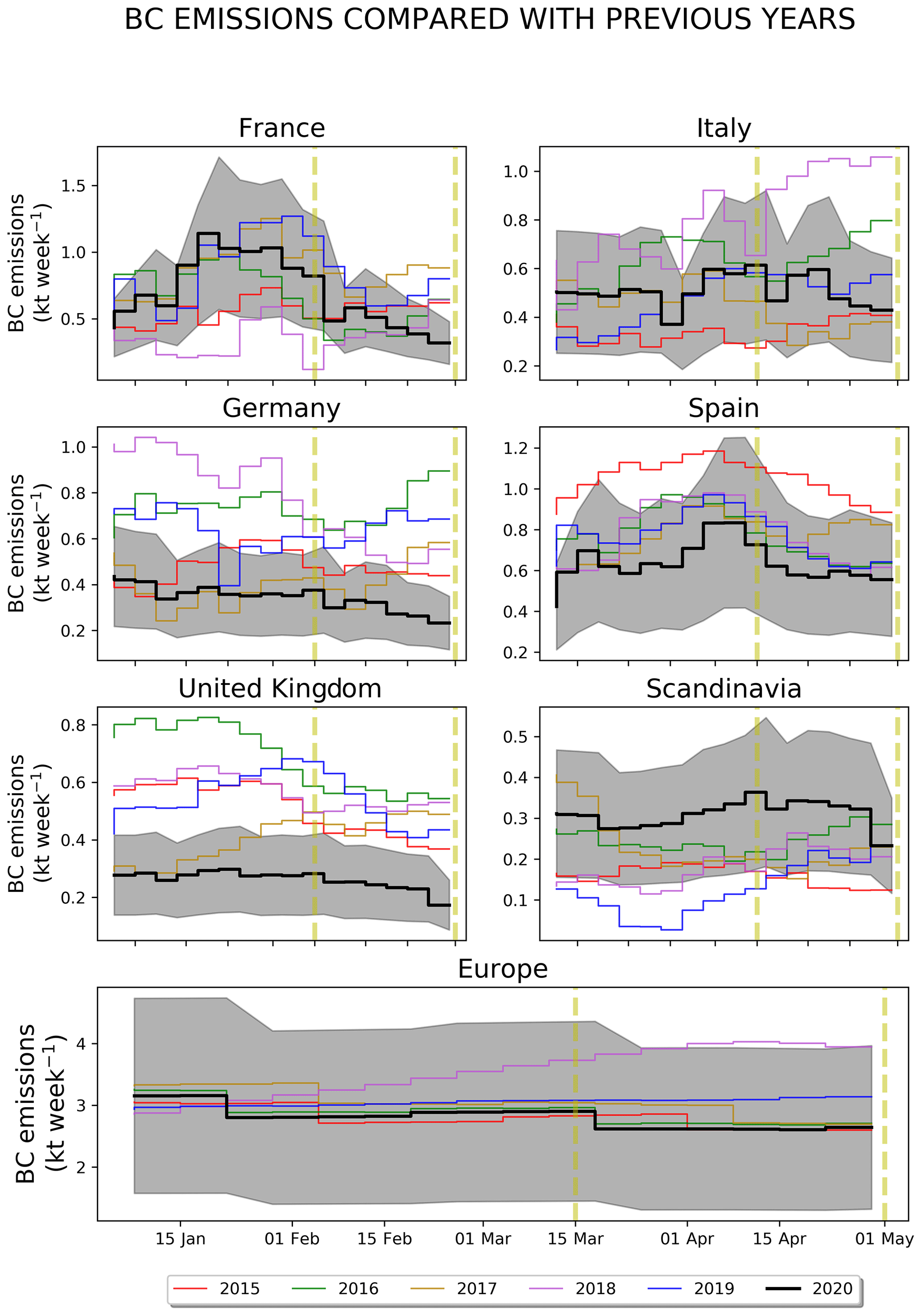
Figure 9 Posterior BC emissions in the most highly affected European countries (France, Italy, Germany, Spain and UK), Scandinavia and Europe by the COVID-19 pandemic (2020). Posterior BC emissions for every year since 2015 are also plotted with the same temporal resolution to show changes in BC emissions characteristics during the 2020 COVID-19 pandemic. The grey shaded area corresponds to the BC emission uncertainty, while the vertical dashed yellow lines correspond to the beginning and end of the 2020 lockdown.

5 Conclusions

The impact of the COVID-19 lockdowns over Europe on the BC emissions, in response to the pandemic, was assessed in the present paper. Particle light absorption measurements from 17 ACTRIS stations all around Europe were rapidly gathered and cleaned to produce a high-quality product. The latter was used in a well-established Bayesian inversion framework, and BC emissions were optimized over Europe to better capture the observations. However, one should be careful not to overinterpret the emission changes at regional scales, due to the poor station data density used and the high-resolution time steps of the inversions (weekly posterior emissions). We calculate that the optimized (posterior) BC emissions declined from 63 to 40 kt (23 %) during the lockdowns over Europe, as compared to the same period in the previous 5 years (2015–2019). The largest reductions were calculated for countries that suffered from the pandemic dramatically, such as Italy (3.4 to 2.7 kt), Germany (3.3 to 2.0 kt), Spain (4.7 to 3.1 kt) and France (3.5 to 2.7 kt). BC emissions in Western Europe during the 2020 lockdowns were decreased from 8.8 to 6.0 kt (32 %), in Southern Europe from 17 to 9.9 kt (42 %) and in Northern Europe from 5.4 to 3.8 kt (29 %) as compared to the same period in the last 5 years. BC emissions were slightly enhanced in Eastern Europe (from 28 to 31 kt) and remained unchanged in Scandinavia during the lockdown, due to increased residential combustion, as people had to stay home and temperatures at that time were the lowest of the last 5 years. The presence of wood-burning aerosols during the lockdowns was confirmed by large MERRA-2 AE values, as well as by absorption AE measurements from AERONET that were higher in the lockdowns than in the same period of the last 5 years. The impact of the European lockdowns on BC emissions was also confirmed by a 11 % decrease of the posterior emissions over Europe during the lockdowns, as compared to the period before, opposite to what was calculated in the previous years, which is obviously due to COVID-19. This decrease was more pronounced in France (42 %), Italy (8 %), Germany (21 %), Spain (11 %), UK (13 %) and Scandinavian countries (5 %). The full impact of the disastrous pandemic will likely take years to assess. Nevertheless, with COVID-19 cases once again increasing in many countries, the information presented here is essential to understand the full health and climate impacts of lockdown measures.