Impact of western Pacific subtropical high on ozone pollution over eastern China

Surface ozone is a major pollutant in eastern China, especially during the summer season. The formation of surface ozone pollution highly depends on meteorological conditions largely controlled by regional circulation patterns which can modulate ozone concentrations by influencing the emission of the precursors, the chemical production rates, and regional transport. Here we show that summertime ozone pollution over eastern China is distinctly modulated by the variability of the western Pacific subtropical high (WPSH), a major synoptic system that controls the summertime weather conditions of East Asia. Composite and regression analyses indicate that a positive WPSH anomaly is associated with higher than normal surface ozone concentration over northern China but lower ozone over southern China. Stronger than normal WPSH leads to higher temperatures, stronger solar radiation at the land surface, lower relative humidity, and less precipitation in northern China, favoring the production and accumulation of surface ozone. In contrast, all meteorological variables show reverse changes in southern China under a stronger WPSH. GEOS-Chem simulations reasonably reproduce the observed ozone changes associated with the WPSH and support the statistical analyses. We further conduct a budget diagnosis to quantify the detailed contributions of chemistry, transport, mixing, and convection processes. The result shows that chemistry plays a decisive role in leading the ozone changes among these processes. Results show that the changes in ozone are primarily attributed to chemical processes. Moreover, the natural emission of precursors from biogenic and soil sources, a major component influencing the chemical production, accounts for ∼ 30 % of the total surface ozone changes.

1 Introduction

Surface ozone is a major trace gas in the lower atmosphere. It is produced by the photochemical oxidation of carbon monoxide (CO) and volatile organic compounds (VOCs) in the presence of nitrogen oxides (NO_x = NO + NO₂) and sunlight. Not only does it act as a greenhouse gas, but it also exerts detrimental effects on both human health and the ecosystem (Heck et al., 1983; Tai et al., 2014; Monks et al., 2015; Fleming et al., 2018; Mills et al., 2018; Liu et al., 2018; Maji et al., 2019). In China, the problem of tropospheric ozone pollution is severe in most urban areas, such as the North China Plain (NCP), the Yangtze River Delta (YRD), and Pearl River Delta (PRD) (Li et al., 2019; Lu et al., 2018; Silver et al., 2018; Yin et al., 2019). Typically, surface ozone concentration reaches its peak in the summer season due to active photochemistry (Wang et al., 2017; Lu et al., 2018). The summertime daily maximum 8 h average (MDA8) ozone concentrations frequently reach or exceed the Grade II national air quality standard of 82 ppbv (parts per billion per volume) in NCP (Lu et al., 2018; Ministry of Environmental Protection of the People's Republic of China (MEP, 2012). Moreover, recent studies showed that surface ozone concentration had exhibited an increasing trend since 2013 over most parts of China (Li et al., 2019; Lu et al., 2020).

Surface ozone concentration is distinctly influenced by meteorological conditions which impact the production, transport, and removal of ozone (Lu et al., 2019a). For example, solar radiation changes surface ozone via the effects on photolysis rates, as well as on biogenic emissions. High temperature tends to enhance ozone pollution through stagnant air masses, thermal decomposition of peroxyacetyl nitrate (PAN), and the increase in biogenic emissions (Fehsenfeld et al., 1992; Guenther et al., 2012; Rasmussen et al., 2012). Wind speed is generally anticorrelated with surface ozone, indicating the important role of horizontal wind in pollutant dispersion (Zhang et al., 2015; Gong and Liao, 2019). Moreover, the variabilities in these meteorological variables are not independent but interconnected. The synchronous variation of some meteorological variables can be ascribed to the same synoptic weather pattern; thus increasing efforts have been devoted to identifying the synoptic weather patterns that enhance ozone pollution (Gong and Liao, 2019; Liu et al., 2019; Han et al., 2020). For example, Liu et al. (2019) objectively identified 26 weather types, including some that led to highly polluted days, and proved that synoptic changes account for 39.2 % of the interannual increase in the domain-averaged O₃ from 2013 to 2017. Han et al. (2020) also identified six predominant synoptic weather patterns over eastern China in summer to examine the synoptic influence of weather conditions on ozone.

A dominant system that affects the summertime weather pattern in China is the western Pacific subtropical high (WPSH). As an essential component of the East Asian summer monsoon, its intensity, shape, and location control the large-scale quasi-stationary frontal zones in East Asia (Huang et al., 2018). The WPSH can significantly influence the monsoon circulation, typhoon tracks, and moisture transport (Choi and Kim, 2019; Gao et al., 2014) and further impact surface ozone in China. Shu et al. (2016) showed stronger WPSHs would increase ozone pollution over YRD by enhancing the ozone production, as well as trapping the ozone in the boundary layer. Using observations from 2014 to 2016, Zhao and Wang (2017) indicated that stronger WPSHs in summer lead to a decrease in surface ozone in southern China but an increase in northern China through statistical analysis. While these studies arrived at qualitative conclusions, they either focused on a limited region or a short time span, and both lacked a comprehensive investigation of the mechanisms through model simulations. Considering the increasingly severe ozone pollution in China, it is desirable to further investigate this topic systematically.

For this purpose, this study aims to address how and why summertime surface ozone concentration in eastern China responds to changes in the WPSH. A joint statistical analysis and model simulation using GEOS-Chem is performed to reveal their relationship, as well as to examine changes in the relevant chemical and physical processes, in order to provide insights into the formation of summertime ozone pollution in China and to shed light on ozone simulation and prediction.

2 Data and methods

2.1 Surface ozone and meteorological data

Routine daily monitoring of air quality in China became available in 2013 with the establishment of a national network by the China National Environmental Monitoring Centre. The ozone data follow the standard released by the Chinese standard document HJ 654-2013 (MEP, 2013), and the pollutant concentration data are available at https://quotsoft.net/air/, last access: 15 January 2021. We used hourly surface ozone concentration data for all sites from 2014 to 2018. An ad hoc quality control protocol was developed to remove outliers and invalid measurements (see Supplement and Fig. S1 for examples of outliers). MDA8 was calculated based on the hourly ozone data. We removed the linear trend of the data and converted the data unit from micrograms per cubic meter (µg m⁻³) into parts per billion per volume (ppbv) for further analysis.

Meteorological fields for 2014–2018 were obtained from the Goddard Earth Observing System Forward Processing (GEOS-FP) database (Lucchesi, 2013), which is the current operational met data product from the Global Modeling and Assimilation Office (GMAO). The data are available at http://ftp.as.harvard.edu/gcgrid/data/GEOS_2x2.5/GEOS_FP, last access: 15 January 2021. The meteorological variables used include sea level pressure (SLP), cloud cover (CLDTOT), solar radiation (SWGDN), 2 m temperature (T2M), 10 m zonal wind (U10M), 10 m meridional wind (V10M), total precipitation (PRECTOT), and relative humidity (RH). These variables are 1 h averages except for RH which is 3 h averages. The hourly data are averaged into daily means for further analysis.

2.2 WPSH index and composite analysis

We first used the long-term ERA5 reanalysis SLP data (Hersbach et al., 2019; https://cds.climate.copernicus.eu/, last access: 15 January 2021) to determine the climatology of and variability in SLP over the northwestern Pacific. Figure 1a shows the multiyear averaged summertime SLP field from 1979 to 2018, and Fig. 1b shows its standard deviation. Although the center of the high-pressure system is located over the northeastern Pacific Ocean, it also shows substantial variability over the western Pacific extending to the east coast of China. This western branch has a significant impact on the summer weather patterns over eastern China. Wang et al. (2013) defined a WPSH index to characterize the change in WPSH intensity. It is calculated as the mean of the 850 hPa geopotential height anomaly within the 15–25^∘ N and 115–150^∘ E region (red box in Fig. 1b), where the maximum interannual variability in the WPSH in the western Pacific Ocean is located. Here we adopted the same method to calculate the geopotential height anomaly and divided the anomaly time series according to its standard deviation to obtain a normalized WPSH index. Then we used this index to represent the strength of and variability in the WPSH (Fig. 1c).

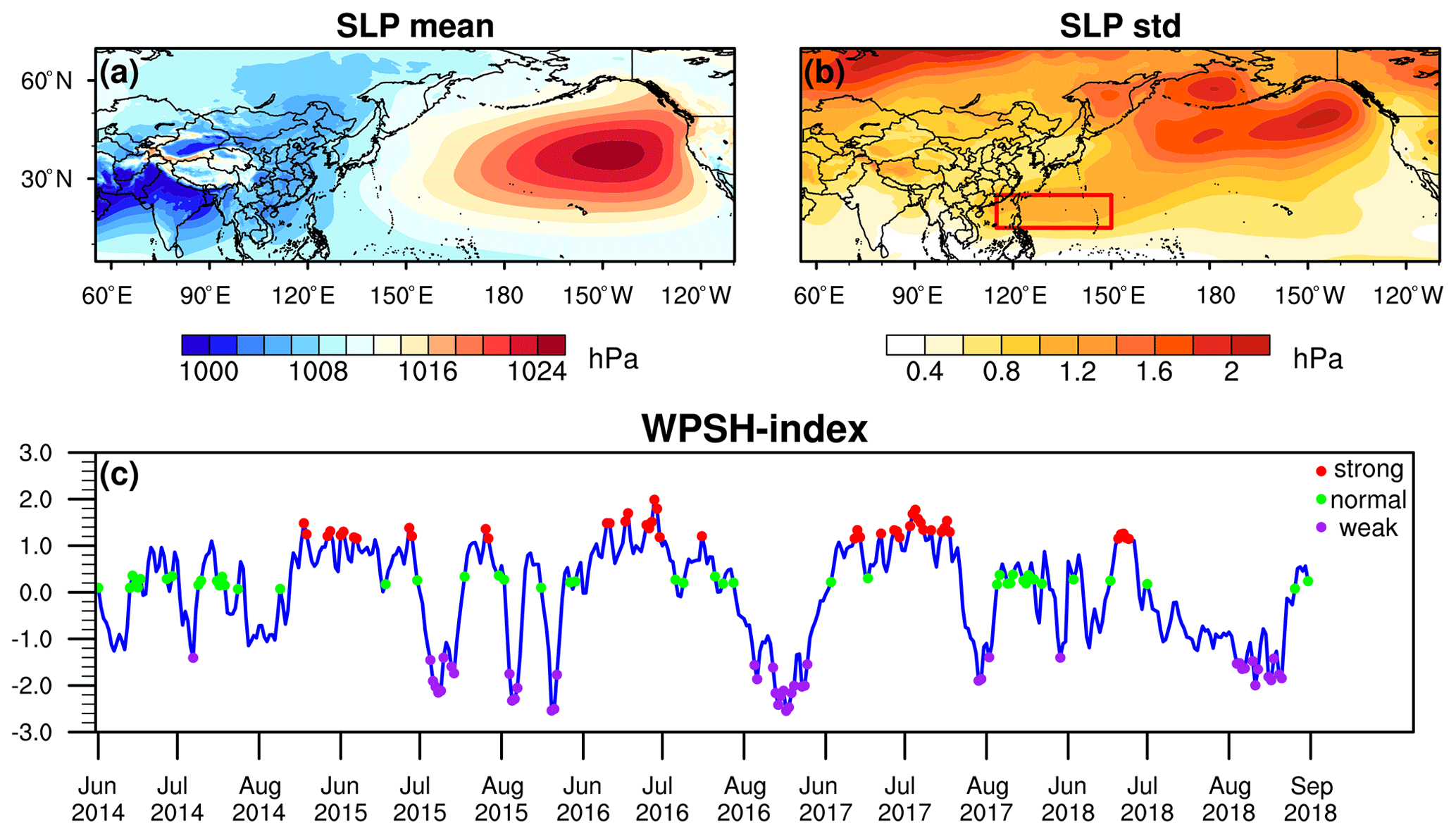
Figure 1 Western Pacific mean sea level pressure (a) and its standard deviation (b) calculated using June, July, and August (JJA) data from 1979 to 2018. Red box in (b) indicates the region (15–25^∘ N, 115–150^∘ E) used to calculate the WPSH index. Panel (c) Shows the time series of WPSH index and the selections of three types of WPSH. The blue line represents the normalized WPSH index of 460 d in JJA from 2014 to 2018. Red dots represent strong WPSH days, green dots represent normal WPSH days, and purple dots represent weak WPSH days.

Using this WPSH index, we defined three types of WPSH conditions, namely strong, normal, and weak. Specifically, days with a WPSH index exceeding the 90th percentile of its distribution are classified as strong WPSH days, the 45th–55th percentiles as normal WPSH days, and those below the 10th percentile as weak WPSH days (Fig. 1c). There are two main reasons for setting this division as the standard: (1) using the 10 % percentile range ensures that we have the same number of days during the summer from 2014 to 2018 for each type and enough samples (46 d for each type) for the composite analysis and statistical test; and (2) the choice of the percentile threshold is to maximize the difference between strong, weak, and normal WPSH conditions in the time span of our study.

Composite analyses of observed and simulated surface ozone, meteorological variables, and related model processes are performed based on these three types. We first calculate the composite mean of each variable for the 46 d of each WPSH type. As we focus on the ozone and meteorology differences induced by WPSH variation, we further calculated and discussed the difference in the composite mean between strong and normal WPSHs, as well as between weak and normal WPSHs. The statistical significance of the difference is tested using the Student's t test. We consider that the two composite means are statistically different if the test result is significant above the 95 % level. All figures except Fig. 1 are displayed in the form of the differences between composite means.

2.3 GEOS-Chem simulations

We use the GEOS-Chem chemical transport model (CTM) (Bey et al., 2001; v12.3.2; http://geos-chem.org, last access: 15 January 2021) to verify the responses of surface ozone in eastern China to changes in the WPSH and to examine changes in the processes involved. GEOS-Chem includes a detailed O_x-NO_x-HC-aerosol-Br mechanism to describe gas and aerosol chemistry (Parrella et al., 2012; Mao et al., 2013). The chemical mechanism follows the recommendations by the Jet Propulsion Laboratory (JPL) and the International Union of Pure and Applied Chemistry (IUPAC) (Sander et al., 2011; IUPAC, 2013). Photolysis rates for tropospheric chemistry are calculated by the Fast-JX scheme (Bian and Prather, 2002; Mao et al., 2010). Transport is computed by the TPCORE advection algorithm of Lin and Rood (1996) with the archived GEOS meteorological data. Vertical transport due to convective transport is computed from the convective mass fluxes in the meteorological archive as described by Wu et al. (2007). As for boundary layer mixing, we used the non-local scheme implemented by Lin and McElroy (2010).

Emissions are configured using the Harvard–NASA Emission Component (HEMCO) (Keller et al., 2014). Biogenic VOC emissions, including isoprene, monoterpenes, and sesquiterpenes, are calculated online using the Model of Emissions of Gases and Aerosols from Nature (MEGAN v2.1; Guenther et al., 2012). Soil NO_x emissions are calculated based on available nitrogen (N) in soils and edaphic conditions such as soil temperature and moisture (Hudman et al., 2012).

The model is driven by GEOS-FP meteorology fields and runs with 47 vertical levels and at 2^∘ × 2.5^∘ horizontal resolution. The model simulations started on 1 January and ended on 31 August for each year during 2014–2018, in which the first 5 months were used as spinup and June–July–August (JJA) were used for composite analysis. Anthropogenic emissions were fixed in 2010, after which the MIX emission inventory (Li et al., 2017) stopped updating so that the differences among the three types of WPSHs are solely caused by the change in meteorology. Because meteorology not only affects the production and transport of ozone but also significantly impacts the emission of biogenic volatile organic compounds (BVOCs) and NO_x from the soil, two important precursors of ozone formation, we also performed another set of simulations with MEGAN and soil NO_x emissions turned off to explore the contribution of natural emissions; in this case, these two emission datasets are not read in during the simulation. We used ozone levels at the lowest model level with an average height of 58 m to represent model-simulated surface ozone concentration.

2.4 Ozone budget diagnosis

The simulated ozone concentration is determined by four processes, namely chemistry, transport (the sum of horizontal and vertical advection), mixing, and convection. Dry deposition is not separately discussed in the budget diagnosis, as this process is included in mixing when using the non-local planetary boundary layer (PBL) mixing scheme. However, as it is an important process for ozone removal, we show the dry deposition flux and velocity at the surface level in the Supplement (Fig. S2). It is found that dry deposition velocity appears spatially correlated with precipitation, i.e., higher precipitation generally corresponds to higher dry deposition velocity, whereas dry deposition flux is proportional to the change in ozone concentrations (Fig. 2). Budget diagnosis is further performed to quantify their individual contributions. GEOS-Chem v12.1.0 or later versions provide budget diagnostics defined as the mass tendencies per grid cell (kg s⁻¹) for each species in the column (full, troposphere, or PBL) related to each GEOS-Chem component (e.g, chemistry). These diagnostics are calculated by taking the difference in the vertically integrated column ozone mass before and after the chemistry, transport, mixing, and convection components in GEOS-Chem. Here we use the budget diagnostics in the PBL column and calculate composite means for each type of WPSH.

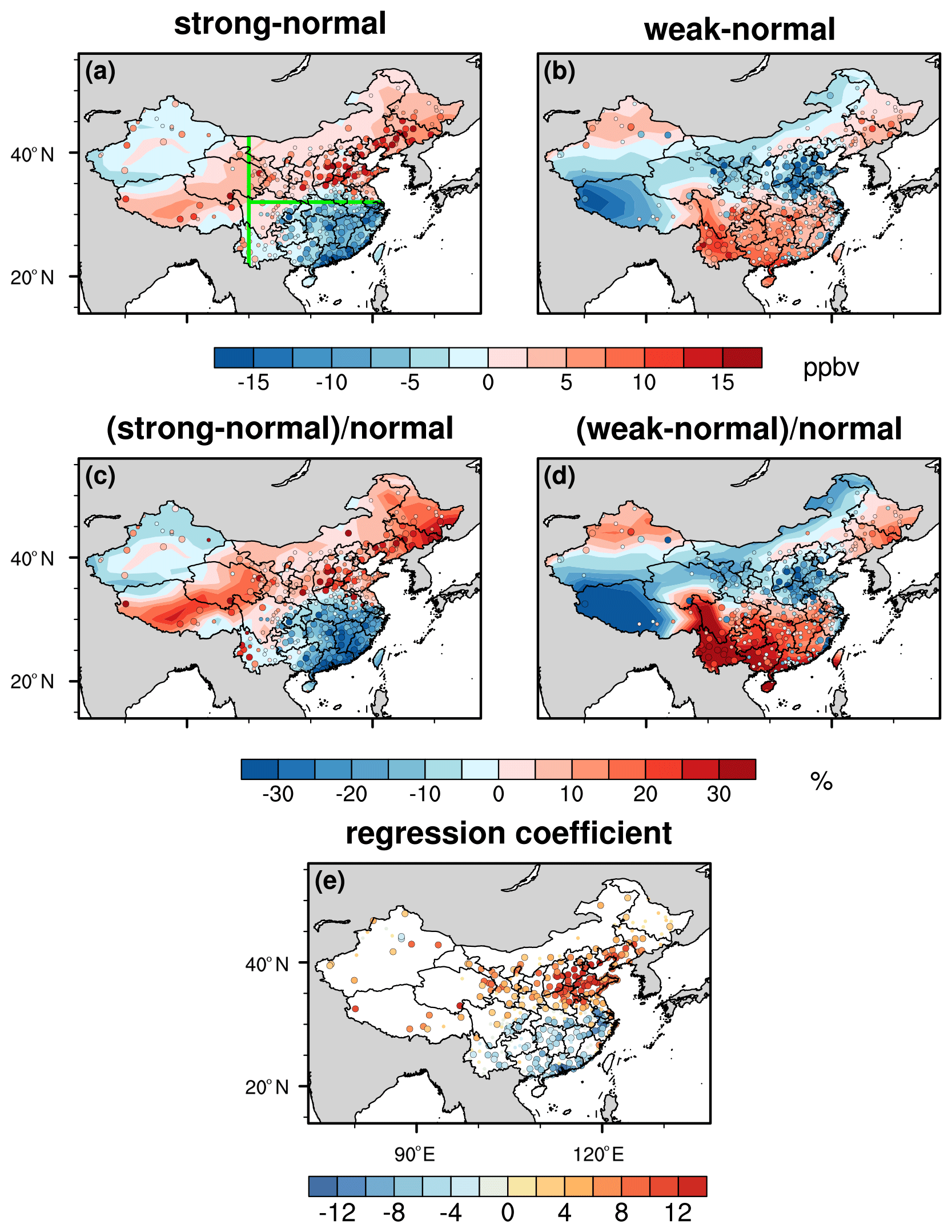
Figure 2 The observed (symbols) and simulated (filled contours) difference in MDA8 (ppbv) during strong and weak WPSH relative to normal WPSH days. (a) MDA8 of strong WPSH minus normal WPSH days and (b) MDA8 of weak WPSH minus normal WPSH days. (c) The percentage change in MDA8 of strong WPSHs relative to normal and (d) the percentage change in MDA8 of weak WPSHs relative to normal. (e) The regression coefficient between MDA8 in JJA from 2014 to 2018 and WPSH index for cities in China. Larger dots with black circles in (a)–(e) are sites with a significance level less than 0.05 from Student's t test. The vertical green line in (a) is the boundary of eastern China and the horizontal green line is the division of northern and southern China.

Regarding the region definition in this study, because in Sect. 3.1 and 3.2 the calculations are all site-based (city average), we applied a single latitude division line of 32^∘ N to separate northern and southern China and a longitude division line of 100^∘ E as a boundary for a rough definition of eastern China (green lines in Fig. 2a). In Sect. 3.3 and later, the paper mainly focuses on the model result analysis, which is grid-based (regional average); thus, we used a northern region and a southern region with the same size and shape to ensure their comparability. The principle with which we chose the northern and southern regions is based on the principle of avoiding the influence of coastline and covering as much land area as possible.

3 Results

3.1 Observed surface ozone changes associated with WPSH intensity

We first examine the relationship between observed MDA8 and WPSH index of all cities in China. Figure 2a and b (symbols) respectively show the difference in the composite mean of observed MDA8 between strong/weak WPSH days and normal WPSH days. A distinct dipole-like pattern can be observed in Fig. 2a, indicating that during strong WPSH events, surface ozone concentration tends to be higher in northern China but lower in southern China, especially the southeast region. The transition from positive to negative changes happens around 32^∘ N (Fig. 2a), which is then used as the division between northern and southern China in this study. In contrast, Fig. 2b, which shows the composite mean difference between weak and normal WPSH days, also exhibits a dipole pattern but is opposite in sign to that shown in Fig. 2a. Quantitatively, 45 % and 31 % of the cities show significant differences (p value < 0.05) in Student's t test for the strong and weak WPSH relative to normal days, respectively. During strong WPSH days, the average MDA8 increased by 10.7 ppbv (+19 %; Fig. 2a, c) in northern China and decreased by 11.2 ppbv (−24 %; Fig. 2a, c) in southern China. Under weak WPSH conditions, the average MDA8 decreased by 10.2 ppbv (−17 %; Fig. 2b, d) in northern China and increased by 4.6 ppbv (+10 %; Fig. 2b, d) in southern China. This dipole change in ozone is also confirmed by a regression analysis of surface ozone against the WPSH index (Fig. 2e), in which 71 % of cities show significant signals (p value < 0.05) with positive coefficients over northern China and negative values in southern China.

Composite and regression analyses jointly prove the robustness of the dipole-like ozone anomaly pattern associated with WPSH variability. It is likely that these changes are driven by changes in meteorological conditions. Therefore, in Fig. 3, we further examine the differences in major meteorological variables associated with WPSH intensity.

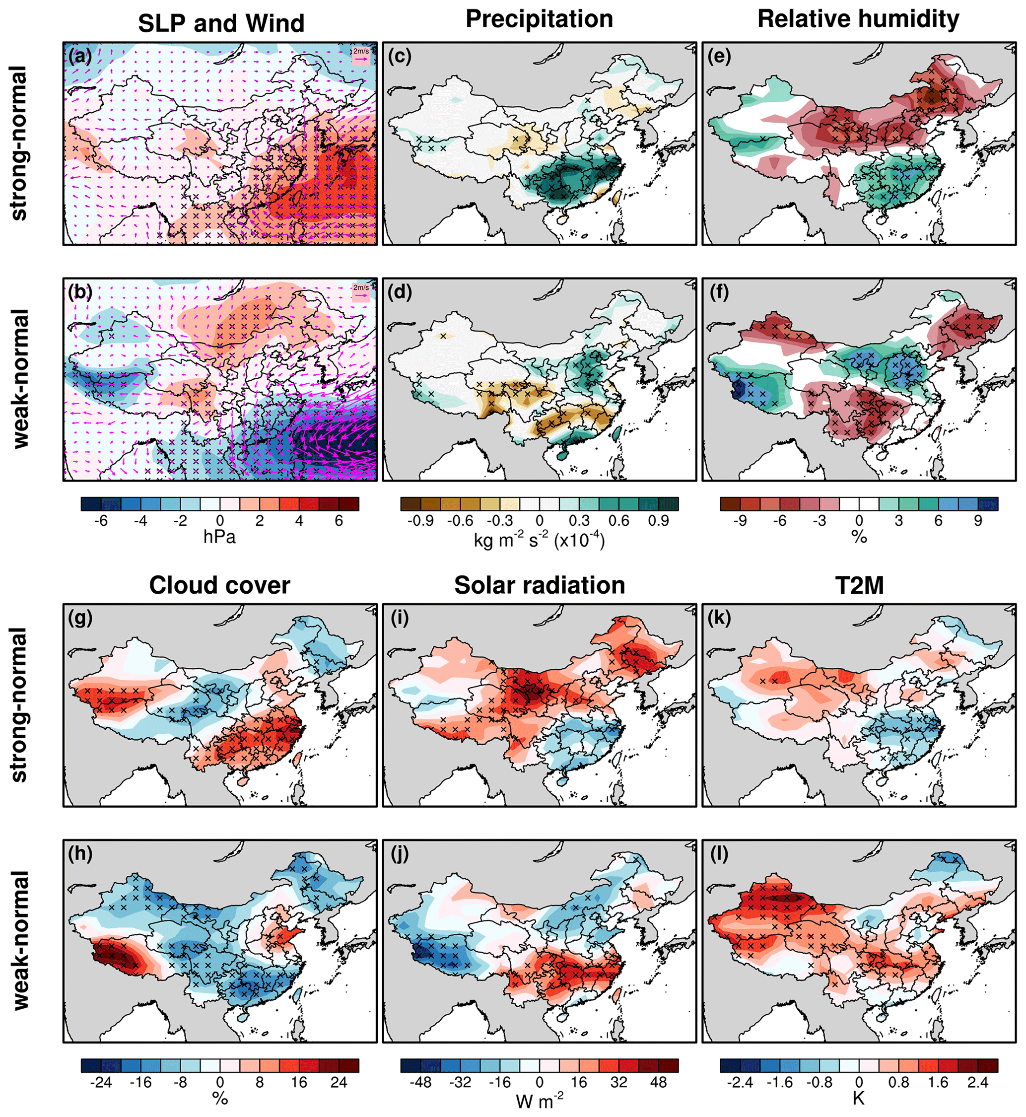
Figure 3 The difference in composite meteorological fields between different WPSH types. The first row corresponds to the difference between strong and normal WPSH days, and the second row corresponds to the difference between weak and normal WPSH days. The meteorological variables including SLP, wind, precipitation, relative humidity, cloud cover, solar radiation, and 2 m temperature. The cross symbols indicate grids with significant levels less than 0.05 from Student's t test.

The change in SLP associated with strong WPSH days clearly shows a positive center in the northwestern Pacific Ocean and to the east of the Chinese coast (Fig. 3a). This high-pressure center induces anti-cyclonic circulation anomalies which manifest themselves as southwest wind (10 m) anomalies over eastern China (Fig. 3a). In northern China, because the surface winds are blown from the land area in the south (Fig. 3a), it contains less moisture but has higher temperatures. As a result, northern China exhibits a decrease in relative humidity (Fig. 3e) and an increase in temperature (Fig. 3k). Although the precipitation does not show significant changes, the decrease in cloud cover (Fig. 3g) increases the near-surface solar radiation (Fig. 3i) and can further change the photochemical reaction rates, which partly explains the increase in ozone concentrations here (Jeong and Park, 2013; Gong and Liao, 2019). The air stagnation associated with higher temperatures and less precipitation may also limit the diffusion and removal of ozone (Lu et al., 2019b; Pu et al., 2017). Moreover, previous studies showed that ozone is negatively correlated with precipitation and RH (Jeong and Park, 2013; Zhang et al., 2015). Among these meteorological variables, RH, solar radiation, temperature, and meridional wind are most closely related to surface ozone concentrations (Fig. S3). In particular, for northern China, the highest correlation (positive) is found between ozone and temperature. For central-southern China along the Yangtze River basin, ozone is most highly correlated with RH, whereas for southern China, wind speed and meridional winds seem to play the dominant role. The latter variable also shows a reversed relationship with ozone for northern (positive) and southern China (negative), highlighting the different characteristics in the regional transport of ozone pollution. The results of our correlation analysis are also consistent with previous studies (Jeong and Park, 2013; Zhang et al., 2015; Gong and Liao, 2019). The overall changes in the meteorological fields in northern China thus act to enhance surface ozone.

In southern China, the south winds bring moisture from the ocean surface, providing ample water vapor for the rain band that forms on the northern boundary of the WPSH (Sampe et al., 2010; Rodriguez and Milton, 2019). This results in increased precipitation (Fig. 3c), relative humidity (Fig. 3e), and cloud cover (Fig. 3g) and reduced surface shortwave radiation (Fig. 3i). The increased precipitation and decreased solar radiation also help to lower the surface temperature (Fig. 3k). The corresponding ozone concentration change is thus negative and opposite to that in northern China. In addition, the transport of ozone-depleted air from the ocean can also dilute surface ozone.

Under the weak WPSH condition, it shows a negative anomaly center in the northwest Pacific Ocean and to the southeast of the Chinese coast (Fig. 3b). The changes in meteorological variables mostly show reversed patterns to those under strong WPSH cases, but some asymmetric features are noticed. For example, solar radiation decreased and total precipitation increased in Guangdong province, contrary to the general solar radiation enhancement and precipitation reduction in southern China. However, these asymmetric changes in meteorology match well the observed decrease in ozone in Guangdong province.

According to the weather anomalies related to WPSH intensity, we summarize two pathways for ozone changes: (1) the relative changes in solar radiation and the associated meteorological variables impacting on the chemical formation of ozone and (2) the transport indicated by wind anomalies serving to enrich or dilute ozone concentration depending on the wind direction. Take southern China as an example. The anticyclonic wind anomalies under strong WPSHs tend to dilute ozone, and the cyclonic wind anomalies under weak WPSHs tend to enrich ozone, which is also confirmed in the budget analysis in Sect. 3.4 below. Alternatively, this wind anomaly pattern drives an opposite change in ozone pollution over northern China.

3.2 Simulated WPSH impacts on ozone air quality

Statistical analysis in Sect. 3.1 only reveals a correlation but not causality. To investigate whether or not the WPSH-related meteorology changes indeed induce the dipole-like ozone change pattern, we perform GEOS-Chem simulations from 2014 to 2018 with anthropogenic emissions fixed in 2010. In this way, the model responses are purely attributed to changes in meteorology.

The model's capability in capturing ozone MDA8 concentrations in China is first evaluated by comparing the simulation results from 2014 to 2018 over all Chinese cities with observation (Fig. S4). GEOS-Chem reproduces the observed seasonal spatial distributions of MDA8 reasonably well. The spatial correlation coefficients (R) between the observed and simulated seasonal mean MDA8 concentrations for summers from 2014 to 2018 are 0.57, 0.59, 0.70, 0.81, and 0.81, respectively. The mean bias (normalized mean bias) between the observed and simulated seasonal mean MDA8 concentrations are in the range of 7.1–9.4 ppbv (13 %–22 %) for summers from 2014 to 2018 (Fig. S5). These evaluation results are comparable to those reported in previous studies (Lu et al., 2019b; Ni et al., 2018) despite the slight differences due to differences in season and sampling, proving the confidence of using GEOS-Chem to simulate ozone concentrations.

Figure 2 (filled contours) shows the simulated MDA8 changes during strong/weak WPSH days with respect to normal days (a, b) and their relative changes (c, d). The simulated strong/normal/weak values were calculated from the same days as the observations. Compared with observed changes (symbols), the GEOS-Chem model reproduces well the dipole-like pattern of ozone change albeit with a slight underestimation especially in northern China. By calculating the average changes in simulated ozone concentration sampled at each city, we find the ozone responses to strong and weak WPSHs are quite symmetric, with the average MDA8 increased by 3.6 ppbv (+6 %) in northern China and decreased by 7.1 ppbv (−12 %) in southern China during strong WPSHs (Fig. 2a), and the average MDA8 decreased by 3.6 ppbv (−6 %) in northern China and increased by 6.6 ppbv (+11 %) in southern China during weak WPSHs (Fig. 2b). Although the WPSH index exhibits an asymmetric feature with the difference between weak and normal days much larger than that between strong and normal days, the responses of meteorological variables appear more symmetric (Fig. 3). This thus leads to a more symmetric change in ozone concentrations (Fig. 2). Therefore, we consider this asymmetric behavior in WPSH strength has a negligible effect in the response of ozone pollution. The slight underestimation of model results compared with observation may come from the model's lack of ability in capturing the peak values of ozone MDA8 (Zhang and Wang, 2016; Ni et al., 2018).

3.3 Budget diagnosis

In order to examine and to quantify the chemical and physical processes that lead to the ozone change, Fig. 4 provides the budget diagnostics of chemistry, transport, mixing, and convection in the PBL column. Chemistry represents the changes in net chemical production, which is determined by the change in reaction rate and the amount of ozone precursors. As the photolysis rate and natural precursor emissions are both influenced by meteorological conditions, the change in chemical production is consistent with the variation in solar radiation and temperature in Fig. 3. Under the strong WPSH condition, ozone concentrations from chemical production exhibit a tripolar structure with increases in northern China and the southern edge and decreases in the Yangtze River basin (Fig. 4a).

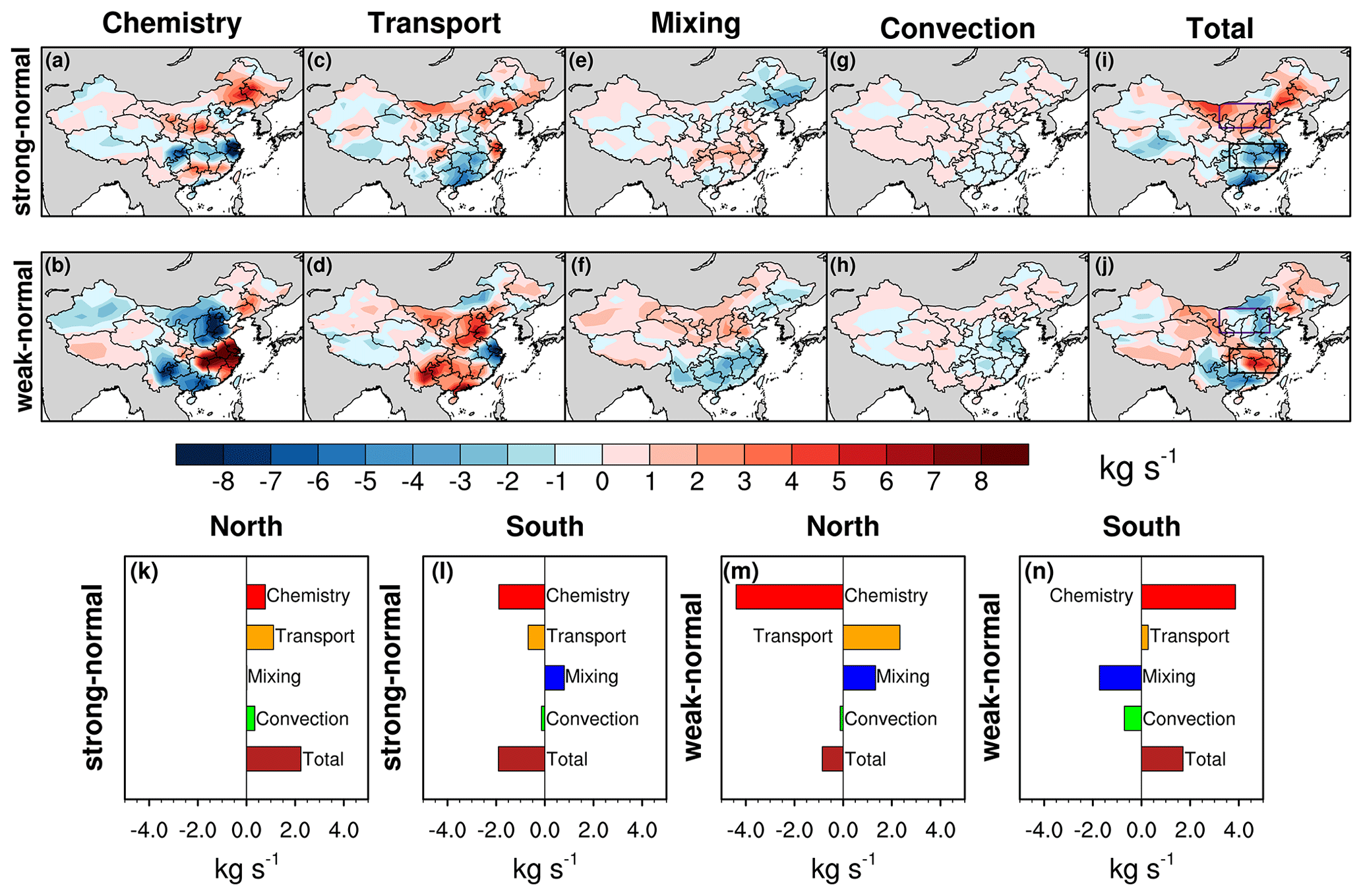
Figure 4 The budget diagnostics (kg s⁻¹) including chemistry, transport, mixing, and convection in the GEOS-Chem model. (a–j) The first row shows the differences between strong and normal WPSH days and the second row shows the differences between weak and normal WPSH days. (k–n) The area-averaged budget diagnostics (kg s⁻¹) for a northern (36.0–42.0^∘ N, 105.0–117.5^∘ E) and a southern (26.0–32.0^∘ N, 107.5–120.0^∘ E) region (purple and black boxes in i and j).

Transport represents the change in horizontal and vertical advection of ozone. For strong WPSHs, the ozone budget due to the transport budget exhibits an asymmetric pattern with decreases in most parts of southern China and increases over northern and northeastern China (Fig. 4c). As the correlation analysis shows that ozone responds to meridional wind positively in the north and negatively in the south (Fig. S3i), the changes in transport budget are consistent with the WPSH-induced wind anomalies (Fig. 3a) which tend to dilute surface ozone in the south and enhance it in the north. The mixing process describes turbulence diffusion in the boundary layer. Mixing in the whole PBL column represents the total exchange in the PBL with the free troposphere, which shows a roughly reversed pattern to chemistry (Fig. 4e). Cloud convection shows a general dipole pattern with positive signals in the north and negative signals in the south. However, the small changes in the absolute value suggest a weak impact via deep convection (Fig. 4g). Under weak WPSH conditions, ozone from chemical production significantly increases in the east of southern China but decreases strongly in northern and southwestern China (Fig. 4b). According to the wind anomalies in Fig. 3b, transport tends to minimize the difference induced by chemistry and thus leads to an opposite ozone change (Fig. 4d). Mixing shows a distinct north–south contrast pattern (Fig. 4f). Convection changes slightly in the opposite direction in the north and south (Fig. 4h). Due to PBL mixing, the total change in these processes (Fig. 4i, j) in the PBL column shows a consistent pattern with both the observed and simulated change in surface ozone (Fig. 2). In general, chemistry (Fig. 4a, b) and transport (Fig. 4c, d) account for the largest proportions of ozone change than the other two mechanisms (i.e., mixing, Fig. 4e, f, and convection, Fig. 4g, h).

In order to provide a more quantitative evaluation of the contribution of these processes, in Fig. 4k–n, we examine the regionally averaged ozone changes for a northern (36.0–42.0^∘ N, 105.0–117.5^∘ E) and a southern (26.0–32.0^∘ N, 107.5–120.0^∘ E) region, respectively defined by the purple and black boxes in Fig. 4i and j. It can be seen that the regionally averaged total ozone change is around ± 1–2 kg s⁻¹. In all cases except northern China under strong WPSHs, chemistry appears to be the dominating process, which results in the largest ozone change and with the same sign as the total change and sometimes can even exceed the amount of total change. For the northern China case, transport slightly outweighs chemistry as the primary factor (Fig. 4k). Transport contributes to total changes either positively or negatively depending on the ozone concentration gradient and wind anomalies. It tends to increase ozone when the wind anomalies come from inland regardless of the direction (Fig. 4k, m, n). In contrast, when the wind comes from the ocean, it serves to reduce surface ozone (Fig. 4l). As the mixing process transports ozone along the vertical concentration gradient, it generally contributes negatively to the total ozone change and thus counteracts excessive chemical changes (Fig. 4l–n). Convection only induces minor modulation to the total changes, generally less than ± 1 kg s⁻¹, and it is negligible for some cases (Fig. 4l, m). There are two possible reasons for this insignificant change. On the one hand, as ozone is insoluble in water, the large changes in convective activities associated with the WPSH variation may only exert a minor effect on the ozone concentration through wet scavenging. Instead, it influences ozone concentration by the vertical transport of ozone, as well as its precursors, but the average change in ozone budget due to convection transport is about an order of magnitude smaller than that due to chemical processes. On the other hand, previous studies show that the effect of convective transport of ozone alone is to reduce the tropospheric column amounts, while the convective transport of the ozone precursors tends to overcome this reduction (Wu et al., 2007; Lawrence et al., 2003). As a result, changes in ozone are neutralized, and the net effect is weak.

3.4 The contribution of the natural emission of ozone precursor gases

In the GEOS-Chem simulation, all anthropogenic emissions are fixed, so there is no anthropogenic contribution to the simulated ozone change. However, the emission of ozone precursor gases from natural sources, primarily biogenic volatile organic compounds (BVOCs) and soil-released NO_x (SNO_x), closely respond to meteorology and further impact the chemical production of ozone, which has been identified as the main driving force of ozone change (see Sect. 3.3). Therefore, in this section, we continue to quantify the contribution of BVOC and soil NO_x emissions to the ozone changes with WPSHs.

Isoprene (used as a proxy of BVOCs) emissions are strongly correlated with temperatures and increase rapidly between 15–35 ^∘C (Fehsenfeld et al., 1992; Guenther et al., 1993); thus, the pattern of their changes with WPSH are highly consistent with the temperature changes (Fig. 5a, b). An intensified WPSH results in 10 %–40 % increases in BVOCs emissions in northern China and 10 %–30 % decreases in southern China, whereas under weak WPSH conditions, they increase strongly in most parts of China but with a slight decrease over the North China Plain and northeastern China. Changes in NO_x emission from the soil also exhibit a similar pattern to those of temperature. Their responses to weak WPSH appear to be stronger than BVOCs, with decreases of up to 40 % over most of northern China (Fig. 5c, d). As most parts of China are the high-NO_x and VOC-limited regions, the overall decreases in BVOCs and NO_x reduce the ozone concentration.

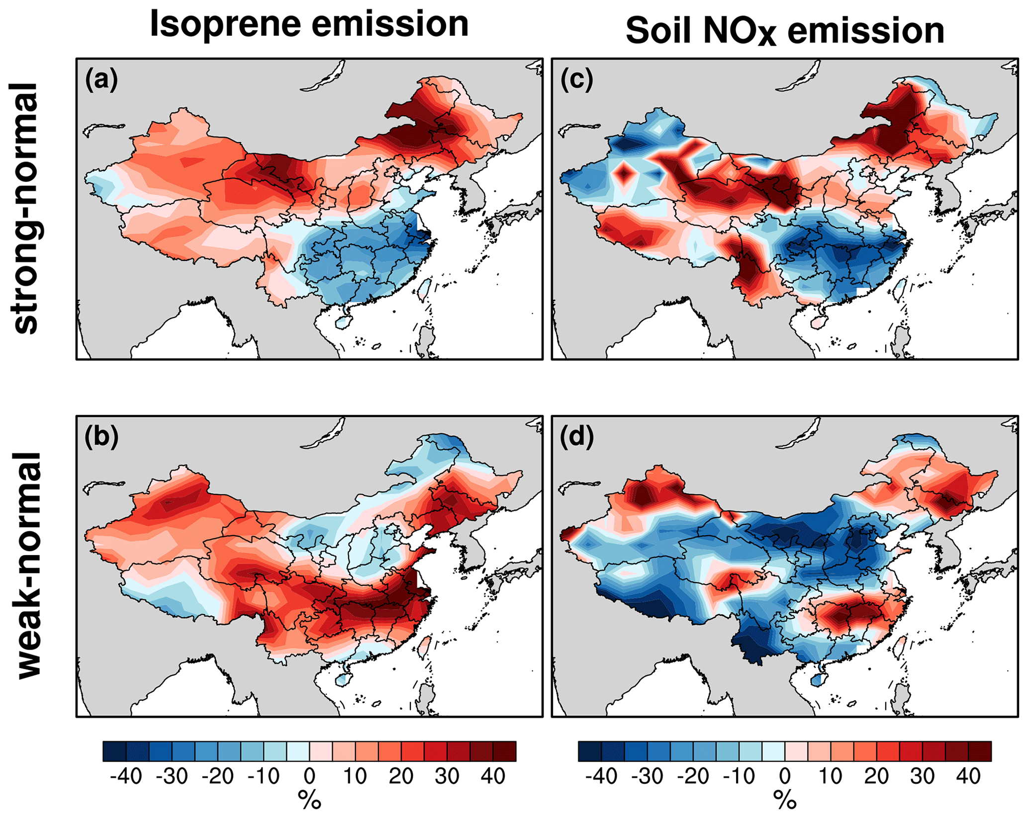
Figure 5 The changes in isoprene (a proxy of biogenic emissions) and soil NO_x emissions in the GEOS-Chem model. Panels (a) and (c) show the relative differences (percentage) between strong and normal WPSH conditions, and (b) and (d) show those between weak and normal WPSH conditions.

Figure 6 Panels (a) and (b) show the simulated difference in MDA8 (ppbv) of strong and weak WPSHs relative to normal WPSHs (same as Fig. 2a, b; filled contours). Panels (c) and (d) are the same as (a) and (b) except turning off MEGAN and soil NO_x emissions. Panels (e) and (f) show the difference between simulations with MEGAN and soil NO_x emissions on (a, b) and off (c, d), which represents the contribution of BVOCs and soil NO_x. Panels (g) and (h) show the difference between simulations with MEGAN emissions turned on and off, which represents the contribution of BVOC emissions. Panels (i) and (j) show the difference between simulations with soil NO_x emissions turned on and off, which represents the contribution of soil NO_x emissions. Note that (a)–(d) use the left color bar and (e)–(j) use the right color bar. (k–n) The contribution of BVOC, soil NO_x (SNO_x), and BVOC with soil NO_x (BVOC + SNO_x) for a northern (36.0–2.0^∘ N, 105.0–117.5^∘ E) and southern (26.0–32.0^∘ N, 107.5–120.0^∘ E) region (purple and black boxes in a and b).

We further quantify the contribution of BVOC and soil NO_x emissions to the changes in surface ozone concentration by comparing simulation results with MEGAN and soil emissions turned on and off. Figure 6a and b and Fig. 6c and d show the simulated MDA8 ozone with biogenic and soil NO_x emissions on and off, respectively. They show similar spatial patterns, but the emission off case exhibits weaker responses. Figure 6e and f show their differences, which represent the MDA8 changes due to the combined effect of BVOC and soil NO_x emission changes associated with WPSH variation. The precursor-induced ozone changes are in phase with the total ozone changes in most parts of China and show a dipole-like pattern. In total, these two factors result in $\sim \pm$ 1.3 ppbv MDA8 ozone changes (averaged over all cities), which accounts for around 30 % of the total simulated change. Figure 6g and h and Fig. 6i and j show the contribution of soil NO_x and BVOC emissions, respectively, from which we can see that the ozone change induced by soil NO_x is weaker, implying that BVOCs are the dominant factor. Figure 6k–n show the averaged contributions from individual and total emissions of BVOCs and soil NO_x for a northern and southern region marked respectively by purple and black boxes in Fig. 6a and b. The averaged ozone changes in the northern and southern regions are in the range of −4 ∼ 4 ppbv, and BVOCs and soil NO_x on average contribute 28 % to the total changes. The combined contribution of BVOCs and soil NO_x is more consistent with that of BVOCs, and the soil NO_x-induced changes are small in all cases except northern China under the weak WPSH conditions. The exception in Fig. 6m might be due to the ratio of VOC to NO_x in the northern region under weak WPSH conditions which shifts towards the NO_x-limited regime, making ozone concentration more sensitive to the change in NO_x. In sum, the result emphasizes the role of BVOC emissions in total chemistry production.

4 Conclusions and discussion

In this study, we highlight the role of weather systems like WPSH on surface ozone pollution in China interpreted with a comprehensive mechanism analysis. The statistical analysis of surface observations reveals a dipole-like ozone change associated with the WPSH intensity, with stronger WPSH increasing surface ozone concentration over northern China but reducing it over southern China and a reversed pattern during its weak phase. This phenomenon is associated with the change in meteorological conditions induced by the change in WPSH intensity. Specifically, when WPSH is stronger than normal, dry, hot southern winds from inland areas serve to increase temperature in northern China but decrease relative humidity, cloud cover, and precipitation, creating an environment that is favorable for surface ozone formation. In southern China, the changes in meteorology and ozone are reversely symmetric to the north. Opposite changes are found during weaker WPSH conditions.

This dipole pattern of surface ozone changes is reproduced well by the GEOS-Chem model simulations, which not only confirms the impact of meteorology on ozone concentration but also allows for the diagnosis of the processes involved in ozone change, namely chemistry, transport, mixing, and convection processes. Our results show that chemistry and transport processes play more important roles than mixing and convection. The transport budget confirms the pattern and quantifies the magnitude of regional transport indicated by the wind anomalies in the meteorological fields. The enormous change in the chemistry budget shows that chemical production serves as the leading process determining the direction of the ozone change. As the anthropogenic emission is fixed, the chemistry process is influenced by the changes in natural emissions and chemical reaction rates associated with WPSH variations. By comparing the GEOS-Chem simulations with the MEGAN and soil emissions turned on and off, we determined that ozone changes caused by natural emissions (including BVOCs and soil NO_x) account for ∼ 30 % of the total ozone changes. The GEOS-Chem simulations in our study serve as a useful tool to provide more quantitative insights and analysis which compensate for the statistical analysis results in previous studies (Zhao and Wang, 2017; Yin et al., 2019).

As WPSH is associated with continental-scale circulation patterns, such as the East Asian summer monsoon (EASM), several previous studies also discussed the impact of the EASM on ozone pollution in China (Yang et al., 2014; Han et al., 2020). However, our study differs from the EASM-related ones in that (1) the EASM has complex space and time structures that encompass the tropics, subtropics, and midlatitudes. Given its complexity, it is difficult to use a simple index to represent the variability in EASM (Wang et al., 2008; Ye and Chen, 2019), whereas the location and definition for WPSHs are more definitive (Lu, 2002; Wang et al., 2013). (2) The influences of the EASM on ozone mainly represent an interannual scale as EASM indices are defined by month/year, while the WPSH is a system more suitable to explore the day to day variability in ozone, which is meaningful for short-term ozone air quality prediction.

A better understanding of the internal mechanism of the WPSH's impact on ozone air quality can also help assess the air quality variation more comprehensively under climate change. The location and intensity of WPSHs keep changing over time; e.g., Zhou et al. (2009) demonstrated that the WPSH had extended westward since the late 1970s, and Li et al. (2012) indicated that the northern Pacific subtropical high would intensify in the 21st century as climate warms. Nonetheless, there still exists a great uncertainty about how the WPSH will change under climate change, and further studies are needed to discuss the responses of ozone to synoptic weather systems like WPSHs in future scenarios. In addition, the variability in WPSHs is found to be related to global climate variabilities such as El Niño–Southern Oscillation (ENSO; Paek et al., 2019) and Pacific Decadal Oscillation (PDO; Matsumura and Horinouchi, 2016). Therefore, how natural climate variabilities like ENSO and PDO interact with WPSH to impact ozone air quality also needs more investigation.