the Creative Commons Attribution 4.0 License.
the Creative Commons Attribution 4.0 License.
 | 18 Feb 2021
Sensitivity of stratospheric water vapour to variability in tropical tropopause temperatures and large-scale transport
Peter H. Haynes
Amanda C. Maycock
Neal Butchart
Andrew C. Bushell
Concentrations of water vapour entering the tropical lower stratosphere are primarily determined by conditions that air parcels encounter as they are transported through the tropical tropopause layer (TTL). Here we quantify the relative roles of variations in TTL temperatures and transport in determining seasonal and interannual variations of stratospheric water vapour. Following previous studies, we use trajectory calculations with the water vapour concentration set by the Lagrangian dry point (LDP) along trajectories. To assess the separate roles of transport and temperatures, the LDP calculations are modified by replacing either the winds or the temperatures with those from different years to investigate the wind or temperature sensitivity of water vapour to interannual variations and, correspondingly, with those from different months to investigate the wind or temperature sensitivity to seasonal variations. Both ERA-Interim reanalysis data for the 1999–2009 period and data generated by a chemistry–climate model (UM-UKCA) are investigated. Variations in temperatures, rather than transport, dominate interannual variability, typically explaining more than 70 % of variability, including individual events such as the 2000 stratospheric water vapour drop. Similarly seasonal variation of temperatures, rather than transport, is shown to be the dominant driver of the annual cycle in lower stratospheric water vapour concentrations in both the model and reanalysis, but it is also shown that seasonal variation of transport plays an important role in reducing the seasonal cycle maximum (reducing the annual range by about 30 %).
The quantitative role in dehydration of sub-seasonal and sub-monthly Eulerian temperature variability is also examined by using time-filtered temperature fields in the trajectory calculations. Sub-monthly temperature variability reduces annual mean water vapour concentrations by 40 % in the reanalysis calculation and 30 % in the model calculation. As with other aspects of dehydration, simple Eulerian measures of variability are not sufficient to quantify the implications for dehydration, and the Lagrangian sampling of the variability must be taken into account. These results indicate that, whilst capturing seasonal and interannual variation of temperature is a major factor in modelling realistic stratospheric water vapour concentrations, simulation of seasonal variation of transport and of sub-seasonal and sub-monthly temperature variability are also important and cannot be ignored.
- Article
(6526 KB) - Full-text XML
- BibTeX
- EndNote


Water vapour concentrations in the stratosphere are very low compared to those in the troposphere but have significant radiative and chemical impacts on the global climate system. For example, stratospheric water vapour changes on decadal to multi-decadal timescales contribute to radiative forcing and surface temperature trends (Forster and Shine, 1999, 2002), as well as to stratospheric temperature trends (Forster and Shine, 1999; Maycock et al., 2014), and can affect tropospheric circulation through stratosphere–troposphere dynamical coupling (Maycock et al., 2013). Stratospheric water vapour also affects ozone, through its effects on HOx radicals (Stenke and Grewe, 2005) and on polar stratospheric clouds (Kirk-Davidoff et al., 1999). It is therefore important to understand the processes that control stratospheric water vapour concentrations and to assess whether or not those processes are adequately represented in the models used for climate projections.
The basic process controlling stratospheric water vapour entry was identified by Brewer (1949). The dominant pathway by which air enters the stratosphere is via transport from the relatively moist upper troposphere through the tropical tropopause layer (TTL) (Fueglistaler et al., 2009) into the lower stratosphere (Holton et al., 1995). The low temperatures in the TTL correspond to low saturation mixing ratios, and air is “freeze-dried” as it is transported to the lower stratosphere, resulting in very low water vapour concentrations (a few ppmv). Precise concentrations depend on the lowest saturation mixing ratios, which depend primarily on temperature but also pressure, sampled by air parcels as they pass through the TTL.
Due to the three-dimensional pathways traced by air parcels, latitudinal and longitudinal variation in the TTL, as well as the vertical variation, are important in determining stratospheric water vapour concentrations (Holton and Gettelman, 2001; Hatsushika and Yamazaki, 2003; Jensen and Pfister, 2004; Bonazzola and Haynes, 2004; Fueglistaler et al., 2004, 2005). This naturally motivates a Lagrangian perspective, in which time histories of saturation mixing ratio of air parcels moving from the troposphere to stratosphere must be considered, with the water vapour concentration entering the stratosphere set by the minimum saturation mixing ratio encountered, commonly known as the Lagrangian dry point (LDP) (Liu et al., 2010). Average concentrations can be estimated by following large numbers of air parcel trajectories, using large-scale wind fields from reanalysis data or from model output, and making simple assumptions about the dehydration process, e.g. that water vapour concentrations adjust rapidly to the local saturation mixing ratio. Such calculations provide useful leading-order insight into seasonal and interannual variation in stratospheric water vapour (e.g. Fueglistaler and Haynes, 2005; Liu et al., 2010; Schoeberl and Dessler, 2011) whilst accepting that important details such as convective-scale transport, mixing and microphysical details that determine particle formation, sedimentation and potential sublimation are omitted.
The nature of the dehydration process means that Eulerian time variability of the TTL temperature field is potentially important in setting average water vapour concentrations. This has been noted by previous authors in the context of equatorial Kelvin waves (Fujiwara et al., 2001), of gravity waves and other equatorial waves on sub-monthly timescales (Kim and Alexander, 2015), and of temporary cooling of the equatorial lower stratosphere associated with stratospheric sudden warmings (Takashima et al., 2010; Evan et al., 2015; Tao et al., 2015). Furthermore, Fueglistaler et al. (2013) showed explicitly from LDP calculations that sub-monthly variations in TTL temperatures have a much larger effect on water vapour concentrations than longitudinal variations in temperature. This conclusion is slightly surprising bearing in mind that the picture of TTL dehydration which has emerged over the last 20 years has tended to emphasise the sampling of the longitudinal variation of temperatures as particularly important in setting water vapour concentrations. Kim and Alexander (2015) showed that sub-monthly time variability of temperatures is underestimated in reanalyses and suggested this is a limitation of dehydration estimates based on such datasets.
Strong interannual variability of water vapour has been observed over the last three decades and is clearly associated with corresponding interannual variability in TTL temperatures (Randel et al., 2004; Fueglistaler and Haynes, 2005). However, along with the interannual variability in temperatures, there are also substantial interannual variations of upwelling velocities in the TTL and hence transport timescales (Ploeger and Birner, 2016; Abalos et al., 2012). An important aspect of the Lagrangian description of TTL dehydration is that the water vapour concentrations entering the stratosphere depend on both the temperature field and transport pathways through the TTL, since it is the combination of the two that determines saturation mixing ratios along trajectories. However, the relative importance of the two effects for variations in water vapour concentrations in the tropical lower stratosphere is not clear. For the observed strong stepwise drop in tropical lower stratospheric water vapour concentrations in late 2000 (Randel et al., 2006; Brinkop et al., 2016), Hasebe and Noguchi (2016) undertook an LDP-based study of variability and concluded the drop was caused by a combination of both anomalously low temperatures and a modification of three-dimensional transport pathways due to weaker horizontal confinement of air masses encircling the Asian summer monsoon. However, their analysis did not include any quantitative separation of the two effects.
Whilst there has been progress in understanding the processes that affect stratospheric water vapour variability and trends, some important questions remain. In particular, the requirements for global climate models to capture the distribution of stratospheric water vapour, its seasonal and interannual variations, and any long-term trends remain unclear. Many current models have systematic biases in TTL temperatures (Kim et al., 2013; Hardiman et al., 2015), and this likely causes biases in stratospheric water vapour concentrations (Keeble et al., 2020). Global models are also likely to be limited by their representation of small-scale dynamical and microphysical processes. Thus, for example, if future changes in stratospheric water vapour were to be driven in part by changes in ice injection into the stratosphere by convective clouds (e.g. Dessler et al., 2016) or by changes in temperature fluctuations associated with gravity waves (e.g. Kim and Alexander, 2015), then global models might fail to capture such changes. The two aspects of dehydration highlighted above – the combined effects of transport and temperatures and the role of time variability in temperatures – are both likely to be important but have not yet been clearly quantified. This motivates the following questions:
-
Is variation in temperatures or in transport more important in determining seasonal, interannual and longer-term variations in water vapour?
-
What is the role of dynamical and hence temperature variability on different timescales in setting water vapour concentrations?
These two questions will be addressed in the following sections using a novel Lagrangian approach that explicitly separates temperature and transport effects. Section 2 describes the datasets and methods used for the calculations. Section 3 describes the results of isolating the roles of temperature and large-scale transport in interannual and seasonal variability of water vapour entering the stratosphere, as well as the impact of sub-seasonal temperature variability, using reanalysis data. Section 4 presents corresponding results for a climate model. Overall conclusions will then be presented in Sect. 5.
2.1 Trajectory and LDP calculations
We calculated Lagrangian dry points and water vapour concentrations using estimates of saturation mixing ratios evaluated across large sets of back trajectories. The back trajectories were calculated using the OFFLINE trajectory model (Methven, 1997; Liu, 2009) taking as input winds, temperatures and diabatic heating rates either from reanalysis data (Sect. 2.2) or from a global chemistry–climate model (Sect. 2.3).
The back trajectories were initialised once a month in the lower stratosphere (see Sects. 2.2 and 2.3 for details) and distributed every 2∘ in longitude and latitude over the tropical region between 30∘ N and 30∘ S, corresponding to 5580 trajectories per initialisation date (results are insensitive to an increased spatial density of initialised trajectories). Each back trajectory was followed for a maximum of 1 year or until it reached the troposphere defined by a potential temperature less than 340 K and a saturation mixing ratio greater than 1000 ppmv. The fraction of trajectories that reach the troposphere within 1 year is typically about 90 %, consistent with previous studies (Liu et al., 2010; Fueglistaler et al., 2013). These are often referred to as “troposphere-to-stratosphere transport trajectories” or “TST trajectories”. For each back trajectory, the time series of temperature and pressure along the trajectory is used to calculate a corresponding time series of saturation mixing ratio. The Lagrangian dry point (LDP) is the location along the trajectory where the saturation mixing ratio is minimum. This gives a water vapour estimate at a space–time location (x0,t0) which can be denoted by SMRLDP(x0,t0), representing the saturation mixing ratio evaluated at the LDP along the back trajectory starting at (x0,t0). The estimate for the tropical water vapour concentration at time t0 is then
where 〈.〉TST represents an average over the set restricted to TST trajectories.
The standard approach to calculating LDPs is to follow back trajectories using contemporaneous velocity fields (including diabatic heating if relevant) and temperature fields. The novel aspect of the calculations presented in this paper is that the relative sensitivity of stratospheric water vapour to temperature variations and to transport variations is assessed by replacing the time series of temperature fields or the time series of wind fields with time series taken from different periods. We use the terms replaced transport and replaced temperature to denote these calculations, and for brevity, we use the term replacement method to describe them together. The difference between the LDPs calculated from these replaced-transport and replaced-temperature approaches and the LDPs calculated from the standard approach may then be used to deduce information on the separate sensitivity to temperature and to transport. Such a separation between temperature and transport is inevitably artificial because in reality aspects of temperature and transport are to some extent coupled, but useful insight emerges. The choice of time series used in the replacement method is described at the start of Sect. 3.1 and 3.2. It should be noted that replaced transport will therefore investigate influences of horizontal and vertical transport without distinguishing between them.
2.2 Reanalysis dataset
The reanalysis dataset used was ERA-Interim (Dee et al., 2011). The trajectories reported in Liu et al. (2010) and Fueglistaler et al. (2013) formed the basis to calculate LDPs in the standard, replaced-temperature and replaced-transport cases. The calculations for ERA-Interim were performed using potential temperature (θ) as a vertical coordinate (with vertical motion relative to θ surfaces specified by diabatic heating), with winds, temperatures and diabatic heating rates provided at 6-hourly intervals at 1∘ × 1∘ horizontal resolution. The trajectories were initialised from the 83 hPa surface on the first of each month. The period considered was 1999–2009, during which there was significant observed interannual variability in lower stratospheric water vapour.
Liu et al. (2010) have noted that lower stratospheric water vapour estimates based on LDPs calculated using ERA-Interim winds, temperatures and diabatic heating rates are significantly lower than observed. This may be, in part, because TTL temperatures in ERA-Interim are lower than in most other reanalysis datasets and satellite observations (Tegtmeier et al., 2020) and also because of the simplified set of processes assumed by the LDP method. Different approaches have been taken when interpreting LDP estimates using ERA-Interim. Liu et al. (2010) found that the addition of a temperature correction of 3 K reduces the bias in both annual mean concentration and in the amplitude of the seasonal cycle. Other authors, for example Ploeger et al. (2013), found the inclusion of empirical corrections to represent the effects of the microphysical details of particle formation, and sedimentation also act to increase the estimates of water vapour concentrations. In this paper, since our focus is on the relative effect of different processes, rather than any comparison against observed values, we simply accept that the predicted water vapour concentrations have a systematic low bias relative to observations. To illustrate this point, and to provide background for the studies to be reported in the remainder of the paper, Fig. 1 shows the average water vapour concentrations predicted by our LDP calculations over the period 1999–2009 together with the corresponding concentrations taken from the Stratospheric Water and Ozone Satellite Homogenized (SWOOSH) database (Davis et al., 2016). The difference between the concentrations is typically about 1.5 ppmv, but the variability and amplitude of seasonal and interannual variation agree well between SWOOSH and the LDP calculation.
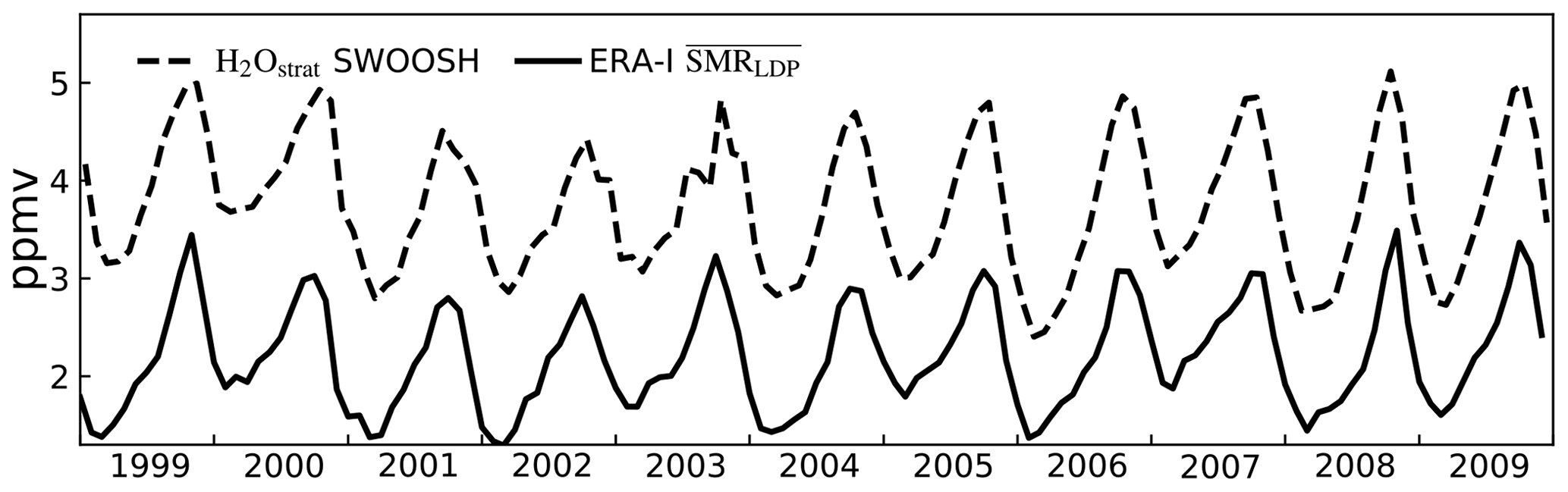
Figure 1Time series over 1999–2009 of monthly mean zonal mean of water vapour in the tropics (30∘ N–30∘ S) at 83 hPa in SWOOSH (Davis et al., 2016) and Lagrangian dry point (LDP) estimates of water vapour entering the stratosphere based on ERA-Interim diabatic back trajectories.
2.3 Chemistry–climate model simulation
The chemistry–climate model used in this study is a version of the Met Office Unified Model with United Kingdom Chemistry and Aerosols (UM-UKCA) based on the Hadley Centre Global Environmental Model 3 (HadGEM3) version 7.3 (Hewitt et al., 2011) with interactive stratospheric chemistry (Morgenstern et al., 2009). The model version was used in Ko et al. (2013). The model is run at N48 resolution (3.75∘ × 2.5∘ longitude–latitude grid) with 60 vertical levels up to an altitude ∼84 km. The model solves the three-dimensional equations of motion with vertical velocity as a prognostic variable. The radiative transfer scheme is Edwards and Slingo (1996) updated to use a correlated-k method (Cusack et al., 1999). The stratospheric chemistry module uses the Fast-Jx photolysis scheme (Telford et al., 2013) and explicitly considers seven chlorine (CCl4, CFC-11, CFC-12, CFC-113, HCFC-22, CH3CCl3, CH3Cl) and five bromine (H-1211, H-1301, CH3Br, CH2Br2, CHBr3) source gases. The model includes a non-orographic gravity wave drag parameterisation scheme and simulates a spontaneous quasi-biennial oscillation (QBO Scaife et al., 2002).
The UM-UKCA simulation analysed in this study is a time slice simulation with perpetual year 2000 boundary conditions for greenhouse gases, ozone depleting substances, HCFCs, aerosols, tropospheric ozone precursor species and orbital parameters. Following Ko et al. (2013), year 2000 sea surface temperature and sea ice boundary conditions are taken as a 10-year average from a coupled ocean–atmosphere HadGEM1 simulation with observed historical external forcings. Therefore, the simulated interannual variability is internally generated within the model. The model is spun up for more than 10 years, and a subsequent 12 years of data are used to calculate back trajectories. This model is generally representative of resolved tropical tropopause and stratospheric processes (Gettelman et al., 2010) but has a warm and wet bias as in other versions of the HadGEM3 climate model (Hardiman et al., 2015). Unlike earlier versions of the UM-UKCA model, the version used here has freely varying stratospheric water vapour that interacts with the radiation scheme. Diabatic heating rate fields were not available from the simulation, and the back trajectory calculations therefore use three-dimensional velocity fields (rather than two-dimensional velocity fields plus diabatic heating). The model uses hybrid height as a vertical coordinate, and some straightforward modifications were required to adapt the OFFLINE code to this. Trajectories were initialised in the middle of each month on the 400 K θ surface. Other details of the LDP calculation were the same as for ERA-Interim.
3.1 Interannual variability
This section examines the relative roles of interannual variation in temperatures and transport in determining observed interannual variation of stratospheric water vapour over 1999–2009. In this time, lower stratospheric water vapour decreased markedly in the period 2000–2001 and remained relatively low for several years (Randel et al., 2006; Rosenlof and Reid, 2008). There were several La Niña/El Niño events during the decade, with the largest El Niño being in 2002–2003 with weaker events in 2004–2005 and 2006–2007, which may have affected stratospheric water vapour (e.g. Gettelman et al., 2001; Bonazzola and Haynes, 2004; Tao et al., 2019).
To assess the relative roles of temperature variations and transport variations in driving interannual variations in stratospheric water vapour, the replaced-transport and replaced-temperature variations are performed as follows. For each month in the period 1999–2009, replaced-temperature LDP calculations use the standard velocity field time series but replace the temperature time series with one shifted forward or backward in time by multiples of 1 year, repeating for all possible choices of the time shift.
The shifts are restricted to multiples of 1 year to take account of the fact that interannual variations are measured relative to a strong annual cycle. To give an explicit example, the standard LDP calculation for January 2004 uses time series of temperature and transport that finish in January 2004. The set of replaced-temperature calculations use the same time series of transport but use temperature time series that finish in January of year X, where the temperature year X is chosen from the set 1999, 2000, …, 2009. Correspondingly the set of replaced-transport calculations use time series of temperature finishing in 2004 but use transport time series that finish in the transport year X.
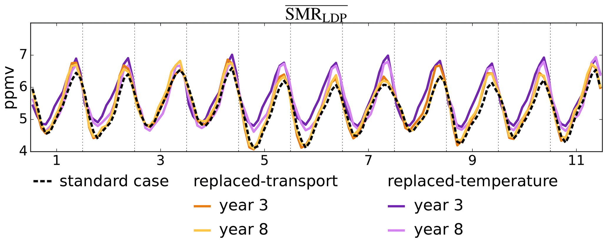
Figure 2a shows the standard (contemporaneous temperature and winds) LDP estimated water vapour time series (black line) and the replaced-transport time series (orange lines) for each of the 11 transport years. Figure 2c shows the corresponding deseasonalised time series as differences from the average annual cycle of the standard case. Note that, by construction, each of the replaced-transport curves in Fig. 2a exactly matches (and is concealed by) the black line during 1 year. The corresponding replaced-temperature LDP estimates are shown as purple lines in Fig. 2b and d.
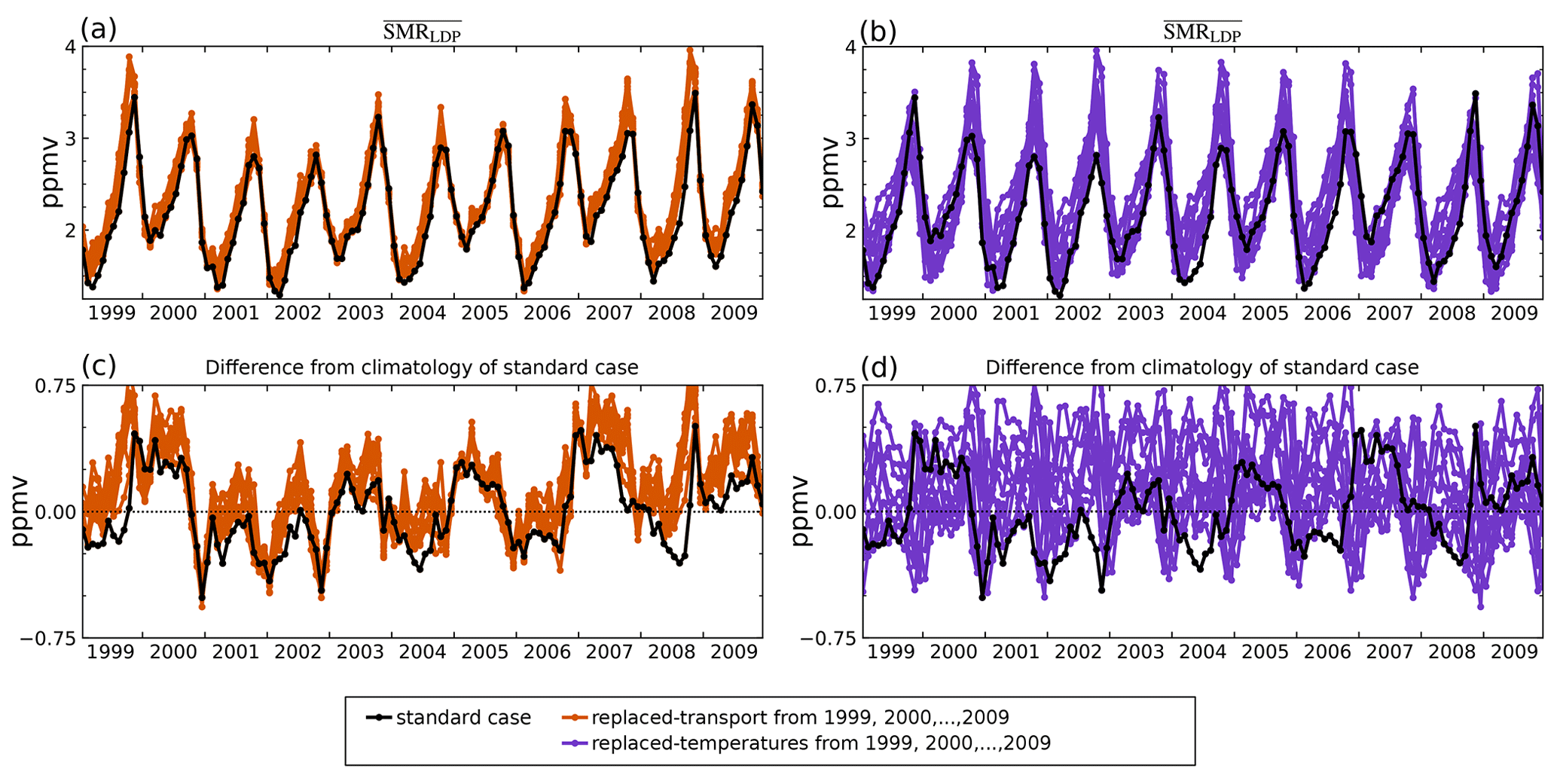
Figure 2Time series of for the standard case (black) and for replacement calculations. The 11 orange lines display cases of replaced transport from each of the other years in 1999–2009, and the 11 purple lines display cases of replaced temperatures. (a, b) Absolute concentrations. (c, d) Anomaly from the mean annual cycle of the standard case.
There is a strong contrast between the estimated stratospheric water vapour mixing ratios from the replaced-temperature and replaced-transport calculations, which is particularly clear in Fig. 2c and d. The interannual variation in the replaced-transport calculations shows much better agreement with the standard calculation than the replaced-temperature calculations. The interannual variation predicted in the standard calculation is typically ±0.5 ppmv. The difference between the replaced-transport calculation and the standard calculation is typically less than 0.2 ppmv and almost always greater than zero. Table 1 shows that the coefficient of determination (R2) between the standard calculation and the replaced-transport calculation is greater than 70 % for all but one (2005) choice of the transport year. The replaced-temperature calculations, on the other hand, show little coherence with the standard calculation, and the R2 value for the two time series is typically 10 % or less.
To give an overall measure of the behaviour of the replaced-transport cases, they are averaged over all choices of transport year except that matching the standard case; this is shown as the orange curve in Fig. 3a. The corresponding average for the replaced-temperature calculation is shown as the purple curve, which represents the mean LDP water vapour over trajectories for the matching calendar year, transported through temperature fields from all replacement years.
Table 1Coefficient of determination (R2) values for the standard and replaced cases in ERA-Interim over the period 1999–2009, and two cases from the climate model simulation. Values are calculated using monthly mean time series with the climatological annual cycle removed.

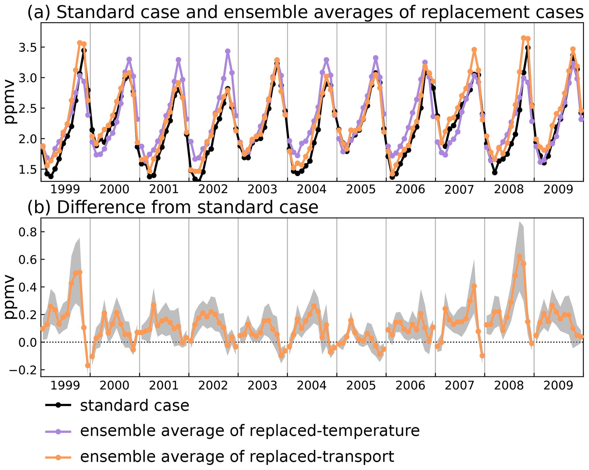
Figure 3(a) Time series of for the standard case (black) and the average across replacement calculations with replaced temperature (purple) and replaced transport (orange). Further described in Sect. 3.1. (b) Difference between replaced-transport ensemble average and the standard case.
In Fig. 3a, the previously identified poor agreement in the replaced-temperature calculation is further demonstrated by the fact that the purple curve shows similar variations from one year to the next, whereas the orange curve captures much of the structure of the interannual variation in the standard calculation. Figure 3b shows the difference between the average of the replaced-transport calculations and the standard calculation, with the climatological annual cycle removed. The fact noted previously that the difference is typically less than 0.2 ppmv is evident, but it can be seen that there are 2 anomalous years, 1999 and 2008, in which the differences are significantly larger, implying that the combined variation of temperatures and transport is important in those 2 years. Both 1999 and 2008 began relatively dry, followed by a transition to relatively wet conditions late in the year. Note that the largest difference between the replaced-temperature calculations and the standard calculation in both of these years is in the July–October period.
Figure 3b shows some interesting seasonal variations in the differences between the replaced transport and the standard calculations with a pattern that applies across most of the 1999–2009 period. The average difference is typically very small in the October–January period and tends to be largest in June–July (though the detailed structure of the time variation is different from year to year). The difference between the replaced transport and standard calculations is predominantly positive, suggesting that the combination of contemporaneous transport and temperatures in a given year is efficient at sampling low temperatures relative to transport of replacement years through the same temperature field. But this efficiency does not apply in the October–January period, and indeed the difference during that period is negative in some years.
The overall conclusion from the above results is that variation in temperature is the main driver of year-to-year variability in stratospheric water vapour entry, accounting for more than 70 % of the interannual variation. However, in certain years, and on the basis of the limited record analysed here, these tend to be a subset of years that are relatively dry, and the combination of temperatures and transport together is important for capturing the observed water vapour fluctuations.
As noted previously, there is a noticeable decrease in stratospheric water vapour in late 2000 which has been the focus of several papers (e.g. Randel et al., 2006; Rosenlof and Reid, 2008; Fueglistaler et al., 2013; Hasebe and Noguchi, 2016), not least because, looking at longer timescales, it marks a transition between a relatively moist period prior to 2000 and a relatively dry period after 2000. Hasebe and Noguchi (2016) made a detailed trajectory-based study of the late 2000 drop in which they identified spatial redistribution of Lagrangian dry points for this period relative to the same period in preceding years. They associated this redistribution with the combined effects of reduction in the strength of the south Asian monsoon circulation and of changes in the spatial distribution of TTL temperatures. However, without further analysis a given LDP redistribution cannot be attributed to any particular contribution of changes in temperatures and changes in transport. The results in Figs. 2a, c and 3b show that both standard and replaced-transport calculations capture the reductions in 2000–2001, with little variation of the result across the choices of year for replaced-transport calculations. That water vapour variation has been demonstrated to be relatively less sensitive to transport than to temperatures indicates that the changes in TTL temperatures were the primary driver for the drop in water vapour in late 2000.
3.2 Annual cycle
This section considers the role of temperatures and transport in setting the annual cycle in stratospheric water vapour using the method discussed in Sect. 3.1.
First, some detailed diagnostics from the standard calculation with contemporaneous temperatures and transport are discussed. These diagnostics are constructed from the same LDP calculations over the period 1999–2009 as in Sect. 3.1 but focusing on the average properties of the annual cycle rather than interannual variation.
Figure 4 shows characteristic features of the ERA-Interim LDP calculations associated with the average annual cycle in tropical lower stratospheric water vapour. This expands on the results shown in Fig. 6 of Fueglistaler et al. (2013). Figure 4a shows water vapour at 83 hPa in SWOOSH observations (black dotted line) and the prediction from back trajectories initialised at that level (solid black line with coloured diamonds marking each initialisation date). In the SWOOSH data, a clear annual cycle is seen with a minimum in March/April of around 3 ppmv and maximum in November of 4.8 ppmv, i.e. a peak-to-peak amplitude of 1.8 ppmv. The calculation shows a very similar phase, with a minimum of 1.7 ppmv and maximum of 3.1 ppmv, i.e. a peak-to-peak amplitude of 1.4 ppmv. The dry bias and the reduced annual cycle amplitude of , the latter consistent with the non-linearity of the Clausius–Clapeyron equation with respect to temperature, relative to observations have previously been noted by Liu et al. (2010).
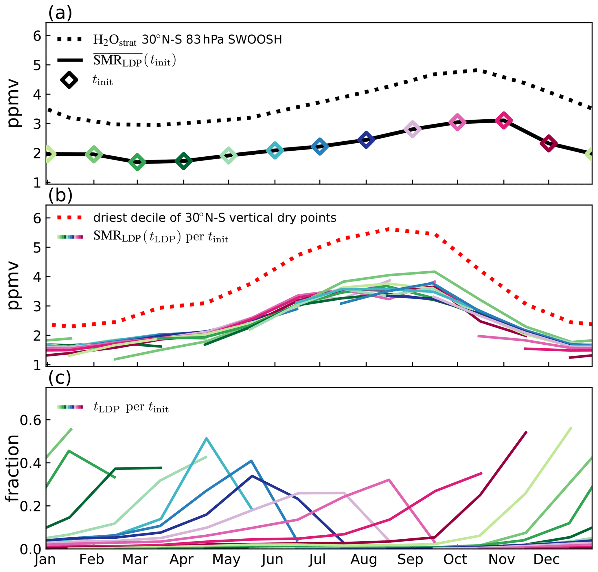
Figure 4(a) Zonal mean tropical (30∘ N–30∘ S) mean 1999–2009 mean annual cycle of water vapour at 83 hPa from SWOOSH observations (dotted) and ERA-Interim LDP estimates (black line) with coloured diamonds denoting initialisation dates. (b) Estimates of water vapour concentration at final dehydration location, LDPs (coloured line for each release date, tinit) and an Eulerian estimate from the driest decile of tropical vertical profiles of saturation mixing ratio (red dotted line). (c) Fractional contribution of LDP events to SMRLDP estimate in each month for each initialisation date (tinit) (colours as in a). Akin to Fig. 6 of Fueglistaler et al. (2013) but showing predicted concentrations from trajectories released within 30∘ N–30∘ S monthly, as well as observations and an additional Eulerian estimate of water vapour. See Sect. 3.2 for details.
Figure 4b shows the seasonal variation of SMRLDP in the 12-month history from each initialisation date, with each coloured line corresponding to a coloured diamond in Fig. 4a. Each line shows the average SMRLDP over the subset of back trajectories for which the LDP is encountered in each month of the set's history. Figure 4b also shows a dotted line which is the average saturation mixing ratio over the driest 10 % of all vertical profiles within the tropics 30∘ N–30∘ S in a given month. The driest 10 % of profiles is determined based on the lowest saturation mixing ratio identified in each vertical profile. (Note that the mean saturation mixing ratio over all tropical profiles is around 9.7 ppmv, which is significantly wetter that the mean of the driest decile.) The dotted line therefore varies roughly in proportion to the saturation mixing ratio associated with the Eulerian mean temperature in the tropics (30∘ N–30∘ S). This Eulerian measure has been used in some papers to approximate the saturation mixing ratio in the absence of detailed trajectory information (see, for example, Garfinkel et al., 2013; Oman et al., 2008). To a large extent the Eulerian and Lagrangian measures show similar seasonal variation, but the efficiency of sampling low saturation mixing ratios by the trajectories is significantly better than the driest decile, as indicated by the lower mean value of the former by 1 ppmv in boreal winter and up to 2 ppmv in boreal summer and autumn. The coloured lines approximately superimpose, indicating that to a large extent the SMRLDP sampled in a particular month does not strongly depend on when the trajectories are initialised in the year.
The for a given initialisation month in Fig. 4a is a weighted average of the values from the equivalent coloured line in Fig. 4b. These weightings are the fraction of LDPs occurring in each of the months preceding the initialisation month, as shown in Fig. 4c. For example, for back trajectories released in August (dark blue line), no LDP events occur in the first month preceding release. The second month preceding release sees around 25 % of LDPs, the third month around 35 % and the fourth month around 15 %, with the fraction reducing systematically further back in time. Taking these weightings into account, it can be seen that the parts of the lines in Fig. 4b that seem to be outliers make only a small contribution to the in Fig. 4a.
For back trajectories initialised in June–October, the largest number of LDPs are found in the second or third month preceding release. For back trajectories initialised in November–May, the largest number of LDPs are found in the first month preceding release. This is likely to be due to a combination of two effects. The first is that tropical lower stratospheric upwelling in the Brewer–Dobson circulation is stronger (Butchart, 2014), and the vertical minimum in temperatures in the TTL is at higher altitudes in boreal winter and spring (e.g. Kim and Son, 2012; Randel et al., 2003); therefore, the transit time from the coldest region to the 83 hPa level is shorter. The second reason is that the seasonal variation in temperatures means that back trajectories released in boreal summer are likely to experience lower temperatures further back in time, hence lengthening the distribution of LDPs backward time, and vice versa for those released in boreal winter.
The seasonal distribution of weights explains why the annual cycle in at 83 hPa in Fig. 4a is distorted in shape relative to the dry point annual cycle in Fig. 4b, with a longer moistening time (April–November) and faster drying time (November–March). The slow increase in spring and summer is due to broader transit time distributions that stretch out this part of the annual cycle signal. Conversely, the narrower distributions in winter give a more immediate signal and hence a relatively rapid decrease in .
We now apply the replacement method previously used in Sect. 3.1 to assess the relative roles of transport and temperatures in determining the annual cycle variation. Here the replaced field is displaced by a given number of months rather than by a number of years. To limit the computational resource of this calculation, we focus on particular months in 2004 to use as the replacement time series. The specific choices are that the replacement time series in velocity (hence transport) or temperatures are initialised in one of the months of February, May, August and November in 2004. As the standard time series are initialised for each month of 11 years and there are eight replacement time series, the total number of LDPs being calculated is about 6×10⁶.
The results for these cases are shown in Fig. 5a and b for replaced-transport calculations and Fig. 5c and d for replaced-temperature calculations. Figure 5a and c show results for a 3-year period, 2003–2005, and Fig. 5b and d show climatologies averaged over all 11 years. The black curve in each case shows the standard calculation with contemporaneous temperatures and transport. Four curves are shown in each sub-panel, corresponding to each month of initialisation of the replacement time series. For example, in Fig. 5a and b the dark brown curve shows the replaced-transport calculation initialised in February 2004 as indicated on Fig. 5a by the matching colour bar. The dark brown curve exactly matches the standard calculation in February 2004 because the shift in the transport initialisation is zero in that month.
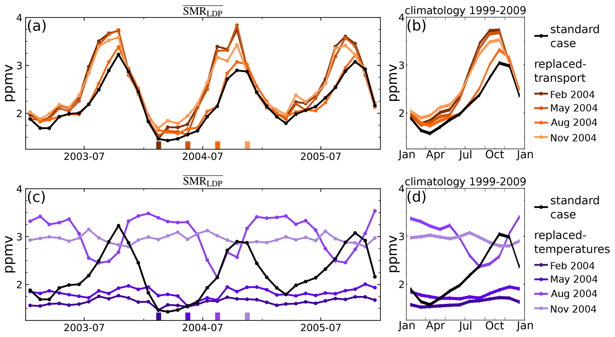
Figure 5(a) Time series of between 2003–2005 for the ERA-Interim standard case (black line) and replaced-transport time series with wind field initialised to a fixed month of 2004 (orange lines); (b) equivalent average annual cycle over 1999–2009. Panels (c) and (d) as for panels (a) and (b) but for replaced-temperature time series with temperature field initialised to a fixed month of 2004 (purple lines). Line shade corresponds to particular months marked with ticks; see also legend.
Figure 5a and b show that with replaced transport the LDP calculation roughly captures the phase of the annual cycle generated by the standard calculation. However, the maximum is significantly overestimated and occurs a month or so early. The largest overestimate of the maximum is for transport initialised in February. The smallest overestimate is for transport initialised in August. Since the orange lines of this figure differ only by replaced transport, and because of the seasonality in upwelling, we can consider an explanation in the contribution of transport pathways to the seasonal distribution of LDPs shown in Fig. 4c. For phases of the annual cycle where SMR values were increasing in previous months, a broader weighting function implies a large contribution from earlier times and hence lower values of SMR averaged over LDPs (Fig. 4b). Of the replaced-transport sensitivities shown in Fig. 5a and b, the broadest weighting distribution is associated with transport initialised in August 2004. This curve shows the smallest overestimate at the annual cycle maximum because the contribution from LDPs during boreal spring was largest. The narrower weighting functions of other replaced-transport combinations also tend to shift the time of the maximum average LDPs towards the time of the maximum saturation mixing ratios in the TTL (that is, away from the time of the maximum in Fig. 4a and towards the time of the maximum in Fig. 4b).
Turning to Fig. 5c and d, the LDP calculation with replaced temperatures cannot reproduce a recognisable seasonal variation, confirming that the annual cycle in is primarily driven by the annual cycle in temperatures. However, the line corresponding to August 2004 initialisation of temperature does indicate that seasonal variation of transport has some effect. For this temperature initialisation date, the has a marked minimum in July–October, with a similar explanation to the replaced-transport calculations discussed above. The transport through the TTL of trajectories initialised in the July–October period is relatively slow (relatively broad distribution of LDP events in Fig. 4c); therefore, they can be influenced by low saturation mixing ratios experienced several months previously. When transport is fast, the is primarily determined by recent values, which for temperature initialisation in August will be determined by TTL temperatures in June and July and give relatively large saturation mixing ratios.
The results therefore imply that it is the larger values of saturation mixing ratio in late boreal summer/autumn that are most sensitive to seasonal variations in transport. This sensitivity arises because the slow transport, which is evident in the seasonal LDP distributions (Fig. 4c), allows a large proportion of pathways to experience relatively low temperatures and hence low saturation mixing ratios in boreal spring, thereby constraining values that already give the maximum in the annual cycle.
3.3 Role of sub-seasonal time variability in tropopause temperature
This section considers the effect on stratospheric water vapour of temperature variations on sub-seasonal timescales, to the extent that these variations are resolved in ERA-Interim data.
Figure 6 shows the structure of TTL temperature and its variability in ERA-Interim on sub-daily to seasonal timescales. The separation of the amplitude of variability on different timescales is made by taking running means of the temperature field at each grid box using different time windows and taking the root-mean-square difference between the time series. Figure 6b shows sub-monthly temperature variability as the difference between 6-hourly data and a 30 d running mean. In the tropics, the sub-monthly temperature fluctuations in ERA-Interim peak along the Equator over Africa, the Indian Ocean and the Maritime Continent. The sub-monthly variability can be divided into contributions from different timescales, as shown in Fig. 7. However, we note that the contributions presented in this way share some dependence because the sum of their individual variances underestimates the total variance.
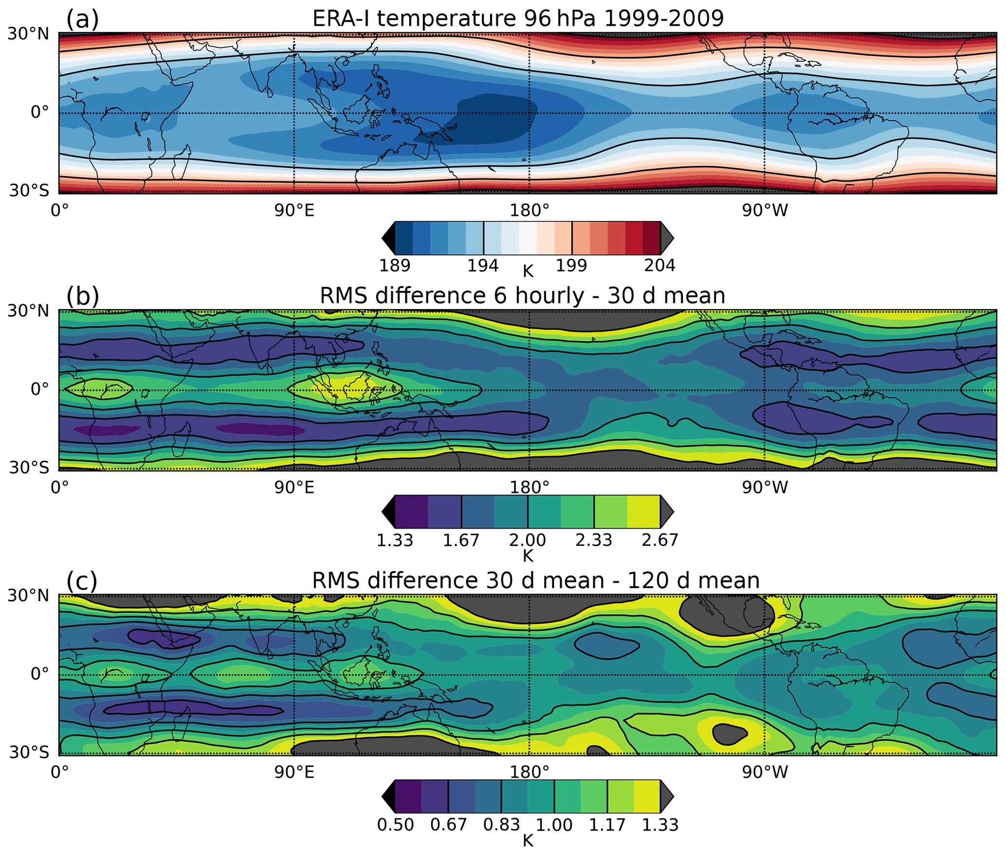
Figure 61999–2009 ERA-Interim temperatures at 96 hPa. (a) Time mean, (b) root-mean-square difference between 6-hourly and 30 d rolling means, and (c) root-mean-square difference between 30 and 120 d rolling means. Note the difference in colour scale between panel (b) and (c).
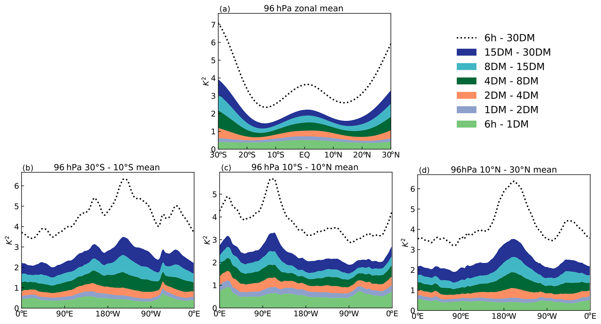
Figure 7Mean square differences between time-filtered ERA-Interim temperatures. (a) Zonal mean 96 hPa time series at each latitude and as a function of longitude between (b) 30–10∘ S, (c) 10∘ S–10∘ N, and (d) 10–30∘ N. Mean square difference between 6-hourly and 30 d running mean (30DM) shown in dotted line, and sub-divisions of sub-monthly timescales (e.g. 1 d running mean to 2 d running mean, 1DM – 2DM) are stacked.
There are many processes that are likely to contribute to TTL temperature variability on sub-monthly timescales. The shortest timescales are likely to be associated with gravity waves generated by convection, with a strong diurnal component (particularly over land) and deep convection (Maritime Continent and western Pacific Ocean) at daily timescales (Johnston et al., 2018); the spatial pattern of regions with higher sub-monthly temperature variability in Fig. 7b appears to be consistent with this. According to analysis of 2–20 d filtered variances by Kim et al. (2019), equatorial Kelvin wave and mixed Rossby-gravity wave activity peaks over east Africa and the east Pacific, respectively. The high sub-monthly variability over the Maritime Continent is also related to 8–30 d synoptic variability (Fig. 7c).
Figure 6c shows temperature variability on the sub-seasonal (30–120 d) timescale for which the Madden–Julian Oscillation (MJO) is likely to be a significant contributor to variability (Madden and Julian, 1994; Virts and Wallace, 2014). Note that the temperature variability associated with the MJO is not confined to the Indian Ocean/western Pacific regions, which tend to be associated with MJO precipitation anomalies, but is also influenced by the dry Kelvin wave excited by those anomalies. See Virts and Wallace (2014) for further discussion. The local magnitude of sub-seasonal temperature variability is typically at least a factor of 2 smaller than the sub-monthly variability. Note that there is significant temperature variability in the subtropics, most likely associated with synoptic systems originating in the midlatitudes and penetrating into the subtropics.
The relative importance of temperature variability at different timescales for stratospheric water vapour depends on the effects on . To quantify this, the LDP calculations along back trajectories are repeated using temperature time series filtered by running means with different windows, as described above. Some previous results on the effect of TTL time variability on have been given by Bonazzola and Haynes (2004), by simply time filtering the Lagrangian temperature time series, and Liu et al. (2010), who considered the effect of imposed Eulerian temperature variability at different timescales. Here, the approach is to control the variability by time filtering the Eulerian temperature fields that the trajectories sample from.
The results of the LDP calculations with time-filtered temperature fields are shown in Fig. 8. As before, the ERA-Interim calculations are for the period 1999–2009. Calculations for UM-UKCA are also shown and will be discussed later in Sect. 4.2. Figure 8a shows the average temperature at LDPs () resulting from the trajectories sampling the smoothed temperature fields, with the timescale of averaging on the horizontal axis. Time mean values are shown as grey circles and the average range of the annual cycle in grey vertical lines. The corresponding blue squares and lines show equivalent results for where space–time locations of LDPs are not re-evaluated from the time-filtered temperatures, but the saturation mixing ratios at that location are calculated with the time-filtered temperature field.
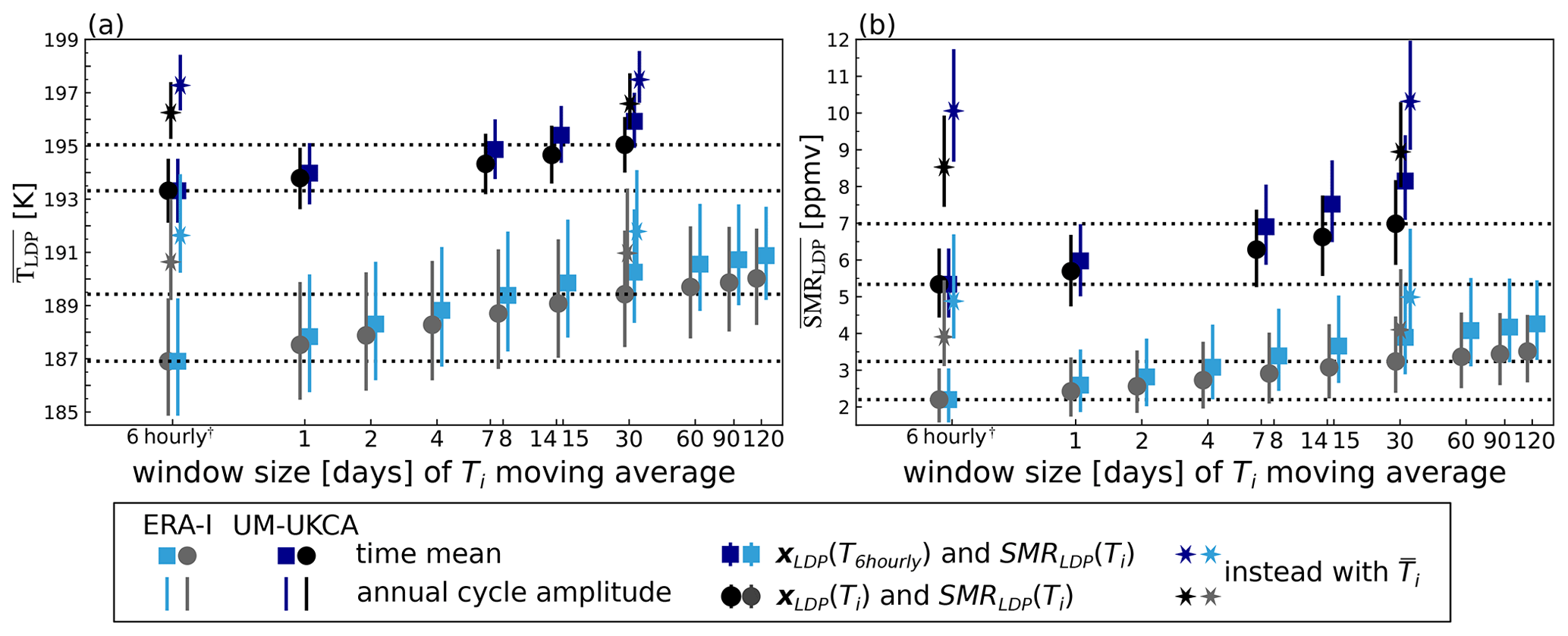
Figure 8Lagrangian dry point calculations for (a) temperature () and (b) water vapour () experiencing different moving-window time averages in ERA-Interim across 11 years (grey and light blue) and the climate model across 11 years (black and dark blue). Showing time mean (points) and mean amplitude of annual cycle (whiskers). Cases of zonal mean temperature are shown as stars. Timescales averaged over include 1 d and 120 d. (†) Note that the 6-hourly temperature field is instantaneous, not averaged. Calculations are divided into those which re-evaluate dry point locations according to averaged temperature field (black and grey data points) and those which fix dry point locations from 6-hourly calculation (blue data points).
Focusing on the grey circles and lines in Fig. 8a, it is seen that if sub-monthly temperature variability is neglected the average increases by 2.5 K (i.e. the difference between the values for 30 d and 6 h). The corresponding difference from neglecting sub-seasonal temperature variability (i.e. on timescales of less than 60 or 90 d) is about 3 K. These differences are consistent with that deduced from LDP calculations by Fueglistaler et al. (2013) (see their Fig. 5a). However, they are much larger than the 0.6 K difference calculated from vertical cold points obtained by removing sub-90 d temperature variability from ERA-Interim temperature profiles, averaging over five sites in the western Pacific (7∘ N, 134–171∘ E across 1990–2014; Fig. 4 of Kim and Alexander, 2015). Part of this difference may be due to the Kim and Alexander (2015) focus on the equatorial western Pacific, which is only one part of the geographical region over which most LDPs are distributed (see Fig. 9). However, it seems likely that an important part of the difference is the sampling effect that is taken into account by the LDP calculation, but which is ignored by considering vertical profiles at fixed locations. By definition, the LDPs are the location of minimum saturation mixing ratio along the trajectories, which implies that cold points corresponding to LDPs will be of very low temperatures relative to the overall distribution of vertical cold points. Averaging temperature differences between those implied by instantaneous temperature fields and those implied by seasonal mean temperature fields across LDPs will therefore almost inevitably give larger negative values than averaging those differences for vertical cold points over a season for all locations in a particular geographical region. A similar effect can be seen in the probability distribution of differences in LDP temperatures arising from a specified addition of random fluctuations to Eulerian temperature fields presented in Fig. 10 of Liu et al. (2010). The probability distribution for the differences in LDP temperature is displaced towards negative values relative to the corresponding distribution for the Eulerian temperature differences.
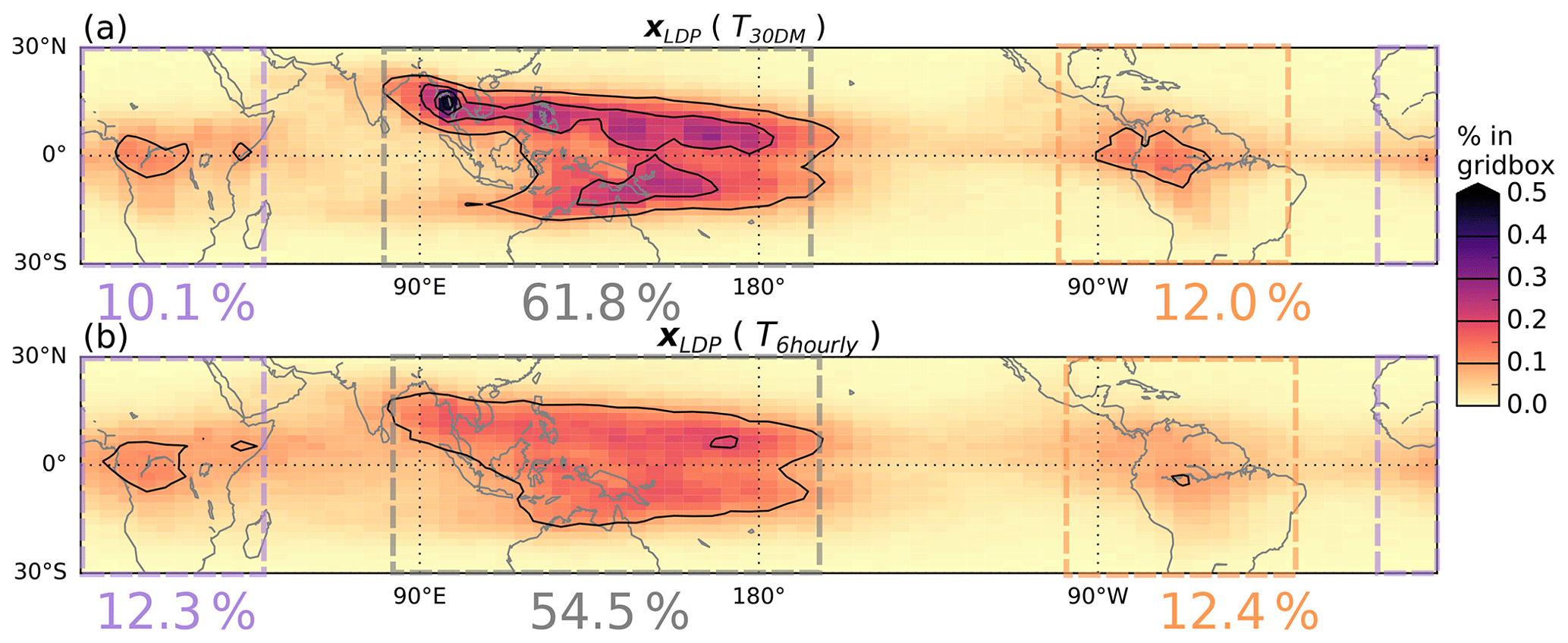
Figure 9Spatial distribution of Lagrangian dry point events for trajectories subject to (a) 30 d mean temperature field and (b) 6-hourly temperatures. The colours show the percent of all LDP events within 4.5∘ × 2∘ grid boxes, with black contours plotted every 0.1 %. The numbers give the cumulative percentages within the coloured boxes.
Figure 8b shows the corresponding predictions resulting from sampling the different filtered temperature fields in ERA-Interim. The previously noted 2.5 K increase in LDP temperatures when sub-monthly temperature fluctuations are omitted corresponds to an increase of slightly more than 1.0 ppmv in . The corresponding increase from neglecting sub-seasonal variability is around 1.2 ppmv. The relationship between average differences and differences is therefore about 0.4 ppmv K−1, consistent with that implied by the Clausius–Clapeyron relation for temperature 190 K and pressure 90 hPa. Further inspection shows that this holds across the 6-hourly to monthly timescales represented by the results shown in Fig. 8. Note that Fig. 8 also shows the effect of time-filtered temperatures on the magnitude of the annual cycle in and . As the time-filtering window is decreased from 30 d to 6 h, the magnitude of the annual cycle in is roughly independent of the sampling, while the magnitude of the annual cycle in decreases by about 15 %. Again, this is what is expected from the dependence of saturation mixing ratio on temperature implied by the Clausius–Clapeyron relation. Note, however, that if the sampling interval is increased to 60 d or longer, i.e. excluding sub-seasonal and sub-monthly variations, the annual cycle magnitudes for both and decrease.
There seems to be no indication from the results that any particular range of timescales has the strongest impact. Rather, there is simply a systematic decrease in and as the temperature time sampling interval decreases. The dependence on timescale appears to be roughly logarithmic; i.e. halving any arbitrarily chosen timescale results in an equivalent reduction in and . Note that the Eulerian measure of temperature fluctuations depicted in Fig. 7 in contrast shows magnitude, which differs with timescale (0.5–1.7 K), but this is less directly relevant to water vapour concentrations.
As previously noted, the time filtering of temperature variability may change the space–time positions of the LDPs. Figure 9 shows the overall effect of time filtering on the distribution of LDP locations, comparing the results from the 6-hourly and the 30 d mean temperature fields. It is clear that removing sub-monthly temperature variability acts to concentrate LDP locations over narrower regions. The LDPs over the west Pacific, the Maritime Continent and Southeast Asia are more geographically confined in the 30 d average case relative to the 6 h case, and there is an overall ∼7 % increase in LDPs in this region (grey dashed box). On the other hand, there is a smaller reduction of ∼2 % in the fraction of LDPs occurring over Africa (purple dashed box) and <1 % change over the tropical Americas (orange dashed box).
The light blue symbols in Fig. 8a and b show results where the LDP space–time locations for each trajectory are fixed to those from the original calculation with the 6 h temperature field (i.e. fixed to those presented in Fig. 9b; conversely, Fig. 9a presents the re-evaluated positions sampled in the case of 30 d mean smoothed temperatures for light grey symbols). By fixing LDP locations the method does not search every trajectory for a new LDP and therefore has lower computational demand. The method is therefore potentially attractive and was used in Fueglistaler et al. (2013). However, by avoiding the search for each trajectory's new saturation minimum based on the new temperature field, the method inevitably leads to a higher time average . From Fig. 8 it can be seen that the impact of using fixed-location LDPs for the ERA-Interim sub-monthly temperature fields is a further increase of 0.8 K in . The total difference between the standard 6-hourly ERA-Interim temperatures and the case with sub-monthly variations removed and without recalculating LDP locations is therefore 3.3 K, which is highly consistent with the 3.2 K reported by Fueglistaler et al. (2013). The corresponding effect on is 0.7 ppmv (a 60 % increase from the full 6-hourly calculation). Therefore, even though the overall spatial distribution of LDPs is changed relatively little by the re-evaluation (Fig. 9), the difference on water vapour abundance is quite substantial, and, for this type of calculation where a replacement temperature field (hence saturation mixing ratio field) is considered, it is clearly desirable that the effect of re-evaluating locations of LDPs is taken into account.
In addition to considering the role of time variability in temperature, we now also consider the role of zonal variation. This is motivated in part by the previous use of zonal mean temperature at a fixed pressure level in the TTL as a proxy for the cold point in the absence of Lagrangian information (e.g. Hardiman et al., 2015) but also because zonal variation of temperature is now regularly invoked in explanations of dehydration. Fig. 8a and b also show time average and values obtained from the along-trajectory sample of the zonally averaged temperature field for the 6-hourly and 30 d mean cases, marked as stars. For 30 d mean temperatures, the effect of zonally averaging temperatures is to increase by about 0.9 ppmv. This case is also about 1.8 ppmv higher than the 6-hourly temperature case with no zonal averaging, indicating that sub-monthly time variability and longitudinal variation account for about equal proportions of the dehydration relative to a zonal-mean monthly average picture.
This section presents results from the UM-UKCA chemistry–climate model described in Sect. 2.3 for comparison with the ERA-Interim results in Sect. 3. Given the absence of interannual changes in boundary conditions in the model simulation (see Sect. 2.3), emphasis here is placed on the seasonal variation and on the role of sub-seasonal and sub-monthly variability.
4.1 Seasonal and interannual variation
The characteristics of the modelled LDPs over the climatological annual cycle are shown in Fig. 10, which can be compared with those for ERA-Interim in Fig. 4. As in Fig. 4, Fig. 10a shows water vapour in the tropical lower stratosphere from LDP calculations and climate model results, Fig. 10b shows Eulerian and Lagrangian estimates of final dehydration saturation mixing ratios, and Fig. 10c shows the relative fraction of LDPs in each month as a function of initialisation date. Modelled tropical mean Eulerian mean water vapour in the lower stratosphere at 80 hPa is shown for comparison in Fig. 10a. The difference between the two curves in Fig. 10a is likely to arise from differences in the transport schemes of the Lagrangian and climate models, as well as processes missing from the simple LDP calculation.
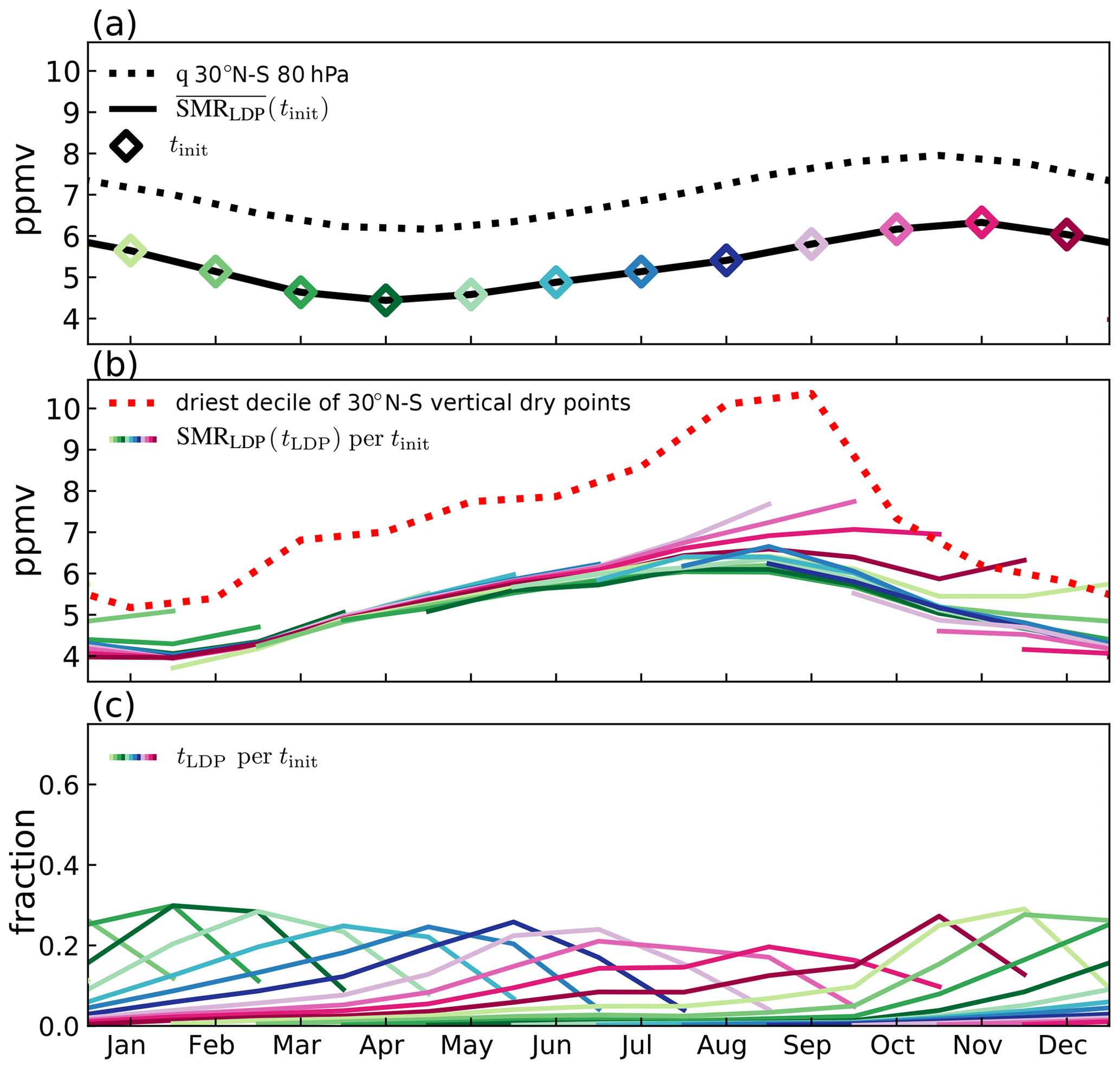
Figure 10Summary results of the LDP method as in Fig. 4 but for 11-year average of the climate model, where the black dotted line is the climate model calculation of water vapour.
As noted in Sect. 2.3, the modelled TTL temperatures are significantly warmer than in ERA-Interim (e.g. 11-year mean tropical and zonal mean temperature at 96 hPa in ERA-Interim is 194.6 K, whereas in the model at 100 hPa it is 199.6 K, implying that saturation mixing ratios will be higher). This difference extends to the lowest decile of vertical dry point saturation mixing ratios shown in Fig. 10b, where the model values are 5–11 ppmv compared to the reanalysis range of 2.5–6.5 ppmv. Correspondingly, the estimate is wetter throughout the year by about 3 ppmv, with an annual cycle minimum and maximum of about 4.5 and 6.4 ppmv, respectively (compared to 1.5 and 3 ppmv for ERA-Interim). The minimum in over the annual cycle is also later by about a month in the model.
While care must be taken in comparing the reanalysis trajectories released from 83 hPa with the model trajectories released from the θ=400 K level, there do appear to be differences in the sampling of temperatures by the trajectories in the reanalysis and model. The fraction of LDPs per month shown in Fig. 10c is lower for the model, reaching no higher than 35 % whereas for the reanalysis the maximum values are typically 50 %. Furthermore, the maximum contribution typically comes from the second to fourth month prior to release (i.e. further into the back trajectory history) rather than from the first or second month. Thus, the for a given month in the model is determined by LDPs distributed over a broader range of times than in the reanalysis. These results suggest that the trajectory transit times from the LDP to the 400 K level in the model are typically longer than from the LDP to the 83 hPa level in ERA-Interim. This may be partly due to two differences. Firstly, the average pressure of LDPs is higher in the model (110 hPa) than in ERA-Interim (94 hPa), indicating a lower altitude and therefore further vertical distance from the initialisation level. Secondly, various measures indicate vertical advection is weaker in the model than in ERA-Interim (for further details, see Smith, 2020).
Another difference between model and reanalysis may be seen from the coloured lines in Fig. 10b. The tails of the saturation mixing ratios for trajectories initialised in boreal autumn and winter show higher values than other curves for the same month, implying that LDPs experienced in the first month or two of trajectory history contribute anomalously wetter LDPs than the average over all LDPs occurring during that period. This behaviour is particularly clear for trajectories released in the September–February period and is not seen in the reanalysis calculation (Fig. 4b). These trajectories must therefore not sample the coldest regions of the TTL efficiently on their path to the troposphere. The model trajectories use vertical velocities rather than diabatic heating rates, and these particular trajectories would have experienced large vertical velocities, perhaps associated with the model representation of vigorous tropical convection that penetrates the TTL. Having noted that uncertainty, it is also important to emphasise that these trajectories are of limited significance for the overall seasonal variation of water vapour concentrations, since they make only a limited contribution, at most 30 % (Fig. 10c), to the monthly mean concentration in the lower stratosphere.
We now consider the roles of transport and temperature variations in setting the average annual cycle in stratospheric water vapour in the model. Figure 11 shows the effect of replaced temperature and replaced transport on the annual cycle for the model simulation; this can be compared with Fig. 5 in Sect. 3.2 for ERA-Interim. The left-hand panels show 3 specific years from the model simulation, and the right-hand panels show the average annual cycle generated from 11 years. As before, the black curve shows the results from the standard calculation with contemporaneous transport and temperature. For the replacement time series, the replacement of temperature or transport is chosen so that the time series are initialised either in February or in August of year 8 of the simulation, corresponding respectively to the drying and moistening phases of the seasonal cycle. For the replaced-transport calculation (Fig. 11a) the overall pattern of over the annual cycle is reproduced, with the minimum value very close to that in the standard calculation, but the maximum value overestimated by about 30 %. However, for the replaced-temperature calculation the pattern of variation is completely lost. For initialisation using February temperatures, the predicted seasonal variation is very weak, whereas for initialisation using August temperatures there is some seasonal variation, with smaller mixing ratios in August and larger mixing ratios in March. These results are broadly similar to those obtained for ERA-Interim (Fig. 5), with some differences in the details. For example, in ERA-Interim initialisation using fixed transport tends to give a maximum saturation mixing ratio that is a month or two earlier than in the standard calculation, but this difference is reduced in the climate model calculation. This may be because the seasonal variation in the fractional distributions of LDPs, as indicated by Figs. 4c and 10c, is stronger for ERA-Interim than it is for the model. This would also explain, for replaced-temperature time series initialised in August, the smaller annual cycle amplitude in the model relative to ERA-Interim (Figs. 11d and 5d). Recalling from Sect. 3.2, in ERA-Interim this variation arises because trajectories initialised in the June–November period sample temperatures over a broader range of times than those in other months, resulting in more efficient sampling and therefore lower . This characteristic is present to some extent in the model calculations but is not as strong as in ERA-Interim.
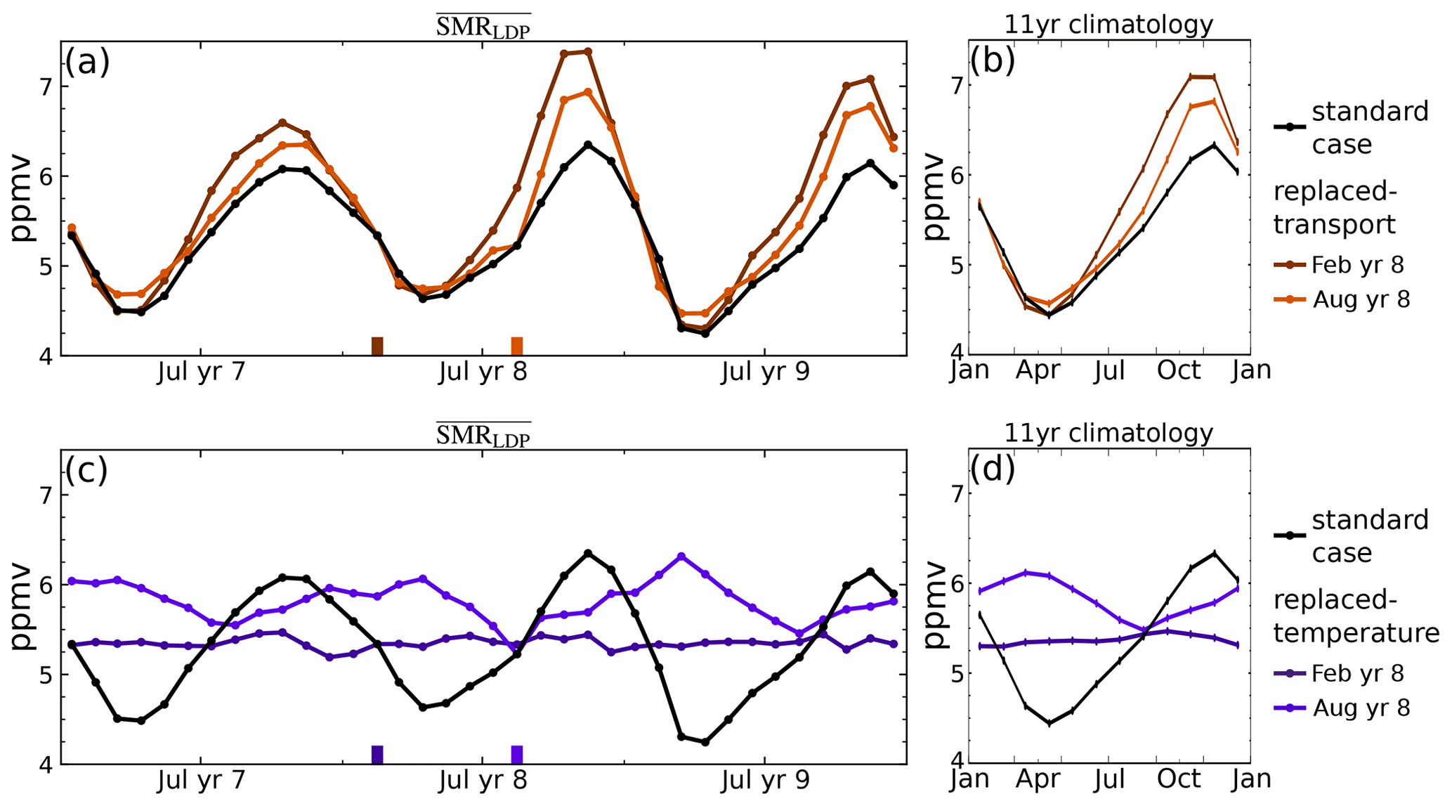
Figure 11As for Fig. 5 but for the climate model. Time series of for 3 years of the UM-UKCA standard case (black line), (a) replaced-transport time series with wind field initialised to a fixed month of year 8 (orange lines) and (b) equivalent average annual cycle over 1999–2009. Panels (c) and (d) as for panels (a) and (b) but for replaced-temperature time series with temperature field initialised to a fixed month of 2004 (purple lines). Line shade corresponds to particular months marked with ticks; see also legend.
As noted previously the model simulation was carried out with fixed boundary conditions and greenhouse gases. There is therefore no external forcing of interannual variability by, for example, sea surface temperature variations. However, there is some internally generated interannual variability, dominated in the tropics by the model's QBO, and there is corresponding interannual variability in stratospheric water vapour. The replacement method used in Sect. 3 may be applied to study the relative importance of temperatures or transport in this variability. Figure 12 shows results of replaced-transport and replaced-temperature calculations, with R2 values reported in Table 1. These results indicate that in the climate model, as in ERA-Interim, it is variability in TTL temperatures that is responsible for the largest part of the variability in water vapour entering the stratosphere. As was found for ERA-Interim, the effect of replaced transport almost invariably overpredicts the simulated water vapour values, but this overestimate is very small for the seasonal minimum in each year.
4.2 Sensitivity to sub-seasonal time variability in tropopause temperature
The examination of the effect of sub-seasonal variations in temperatures on dehydration, reported in Sect. 3.3 for ERA-Interim, is now repeated for the climate model. As before the approach is to construct Eulerian temperature fields smoothed on different timescales and to recalculate the LDPs using the same trajectories as in the standard calculation. The saturation mixing ratios evaluated at the LDPs are likely to change, both simply as a result of the change in the temperature fields and also as a result of the change in the space–time LDP location.
Figure 8a shows in the black and dark blue points comparable results for in the climate model to those previously discussed in Sect. 3.3 for ERA-Interim. Note that some positions on the horizontal axis differ from those of ERA-Interim as not all of the temporal filter window sizes match those applied in the ERA-Interim case. Since the climate model exhibits a warm bias compared to reanalysis, all the points representing the climate model in Fig. 8a (and correspondingly for the saturation mixing ratio results in Fig. 8b) are systematically displaced relative to those for ERA-Interim. However, our focus here is the sensitivity to time-filtered temperatures rather than the absolute values. The difference in time average between the 30 d mean and 6-hourly temperatures is around 1.7 K, compared to about 2.2 K for ERA-Interim. By this measure, temperature variability on sub-monthly timescales is therefore around 20 % lower in the climate model than in ERA-Interim.
Figure 8b shows corresponding results for . The systematic increase in as lower-frequency temperature variability is removed leads to an increase in , as was seen in ERA-Interim. Despite the smaller effect on , the removal of sub-monthly variability leads to a larger increase in of 1.7 ppmv in the model as compared to an increase of 1 ppmv in ERA-Interim. The larger change in in the climate model versus ERA-Interim accompanying the smaller difference in temperatures is due to the non-linearity of the Clausius–Clapeyron relation coupled with the warm bias in the climate model. At higher temperatures, the saturation mixing ratio has a larger temperature sensitivity. The sensitivity seen in the results, about 1.0 ppmv K−1 in the climate model, more than twice that of ERA-Interim, is consistent with a rough estimate from the Clausius–Clapeyron relation, based on a time mean of 193 K for the climate model and 187 K for ERA-Interim.
Also shown in Fig. 8a and b are the results for the climate model for LDP temperatures and saturation mixing ratios obtained with fixed space–time positions of LDPs (dark blue points). The associated difference in is about 1 K and in about 1 ppmv, respectively, which is somewhat smaller and somewhat larger than the corresponding results for ERA-Interim. Interestingly, using zonal mean temperature to calculate LDPs results in an increase in of around 3 K, which is smaller than the equivalent increase in ERA-Interim of around 4 K. This suggests that the zonal variation in temperature in the model is smaller than in ERA-Interim. However, the corresponding increase in in the model is around 3 ppmv, which is considerably larger than the increase in ERA-Interim of 1.8 ppmv. These differences can also be explained by the non-linearity of the Clausius–Clapeyron relation. These results show that mean biases in TTL temperature affect both mean stratospheric water vapour and its variability by creating unrealistic sensitivity to temperature variations across timescales.
Our aim in this paper has been to determine the separate effects of temperatures and transport in determining variations in tropical lower stratospheric water vapour. The motivation is partly to identify to what extent the details of temperature and transport variations need to be represented in models but also to show that insight into the separate effects of temperatures and transport is relevant for understanding observed total variations in stratospheric water vapour.
The technique used in the paper is based on the LDP method but using different combinations of temperature fields and wind fields than in the standard approach where both fields vary contemporaneously. We have used replaced temperature and replaced transport to examine separately the contributions of interannual variations in temperatures and transport to interannual variations in water vapour and also to consider seasonal variation. Such a separation between temperature and transport is inevitably artificial because in reality aspects of temperature and transport are to some extent coupled, but useful results emerge from investigating differences in the replacement time series. Extending some of the results of Fueglistaler et al. (2013), we have used LDP calculations based on time-filtered temperature fields to quantify the role of temperature variability on different timescales in setting concentrations of water vapour in the tropical lower stratosphere.
Regarding interannual variability, our results using ERA-Interim show that interannual variability of temperatures alone reproduces 67–88 % of the total interannual variability of the LDP estimated water vapour over the period 1999–2009. Conversely, interannual variability of transport alone reproduces very little (∼10 %) of the total interannual variability. A similar conclusion is reached for a chemistry–climate model (UM-UKCA), albeit using a time slice simulation where drivers of interannual variability are limited compared to observations.
The differences in saturation mixing ratio between the replaced-transport and standard calculations are mainly positive, indicating that the replaced transport is systematically less efficient at sampling low temperatures. In most years, the largest differences occur in boreal summer and early autumn. In the period 1999–2009, 3 years (1999, 2007 and 2008) show unusually large differences in saturation mixing ratios between the standard and replaced-transport calculations, with differences of up to 0.4–0.6 ppmv in boreal late summer and early autumn coincident with the seasonal cycle maximum. In these years the combination of temperature and transport variations appears to be particularly important for capturing the observed variation in stratospheric water vapour. As noted previously, the year 2000 exhibited an unusual drop in stratospheric water vapour. Our results show that accounting for variations in temperatures alone is sufficient to reproduce this drop in the standard LDP calculation to within 0.1 ppmv. This contrasts with the results of Hasebe and Noguchi (2016) that the combination of both temperatures and transport was responsible for the 2000 water vapour drop.
With respect to the annual cycle, the sensitivity test has shown that the seasonal variation of temperatures rather than transport sets the overall pattern of LDP saturation mixing ratio. The replaced-temperature calculations completely miss the overall structure of the annual cycle but reveal a role for the relatively weaker lower stratospheric upwelling in boreal summer, which means the saturation mixing ratios in late boreal summer are determined by LDPs distributed over several previous months extending back to spring; this results in smaller saturation mixing ratios than if the LDPs were confined to summer alone. The seasonal role of large-scale transport (as seen in Figs. 3b and 5) can be due to the interannual variability of summer monsoons and associated horizontal transport but is not demonstrated here. The seasonal variation of transport – both vertical and horizontal – therefore plays an important role in reducing the maximum in the annual cycle of saturation mixing ratios relative to what can be inferred from the seasonal variation and amplitude in Eulerian measures of cold point temperatures alone. This reduction is counter to the emphasis in some previous papers (e.g. Bannister et al., 2004; James et al., 2008), which have argued that summer-time transport has a moistening effect by allowing pathways from the troposphere to stratosphere that avoid the regions with the lowest saturation mixing ratios. The generally stronger role for transport in determining water vapour concentrations in boreal summer and autumn is consistent with the seasonal variation in the amount of interannual variability captured by the replaced-transport sensitivity calculation noted previously (Fig. 3b).
Decoupling the time variation of temperatures and transport in this way is an artificial approach and could be justified as realistic only if temperatures and transport were truly independent, which they are not. One important basic dependence is between temperatures and diabatic upwelling rates, particularly on seasonal and longer timescales. It is difficult to find a clear argument that the dependencies between temperatures and transport will inevitably lead to more efficient sampling of low temperatures than would be the case if the two were independent, not least because it is the time history of trajectories over periods of months that is relevant. Nonetheless, the replaced-transport calculations, for both the reanalysis and model on interannual and seasonal timescales indicate an apparently robust result that replaced transport tends to give less efficient sampling of low temperatures and consequently higher saturation mixing ratio estimates.
Time filtering was used to quantify the impact of sub-seasonal (30–120 d) and sub-monthly (6 h–30 d) variability in TTL temperatures on stratospheric water vapour concentrations. When sub-monthly fluctuations are included, ERA-Interim estimates of LDP averages are 2.5 K colder and 1 ppmv drier. The corresponding differences in the model estimates are 1.7 K cooler and drier by 1.7 ppmv. Differences for ERA-Interim when sub-seasonal timescales are included are 0.6 K cooler and 0.3 ppmv drier. The results for both the reanalysis and model indicate that there is no particular range of timescales that has a dominant effect – it is simply that LDP temperatures, and consequently mixing ratios, decrease systematically as shorter timescale variations in temperature are resolved. However it should be remembered that the significance of very short timescale variations will in reality be limited by the fact that, at such timescales, the simplifying assumption that water vapour instantaneously relaxes to the local saturation mixing ratio becomes less relevant.
The different quantitative relationship between LDP temperature differences and LDP saturation mixing ratio fluctuations of the climate model relative to ERA-Interim can be explained by the non-linearity of the Clausius–Clapeyron relation and the model warm bias. Note that if the smaller effect of sub-monthly timescales on LDP temperatures in the climate model versus ERA-Interim is interpreted as an underestimate of dynamical variability, then the associated bias in LDP mixing ratios is about 0.8 ppmv or around 25 % of the moist bias in the climate model relative to observations. The implication of this is that, in addition to mean temperatures, the representation of sub-seasonal and sub-monthly time variability of TTL temperatures is important for a model to simulate realistic stratospheric water vapour concentrations under current conditions. Kim et al. (2013) noted that most models of the Coupled Model Intercomparison Project Phase 5 (CMIP5) fail to simulate realistic intraseasonal temperature variability, so this will contribute to the significant mean biases in stratospheric water vapour in climate models.
Kim and Alexander (2015) also demonstrated a qualitatively similar effect of temperature variability on tropical cold point temperatures and hence on dehydration. However, Kim and Alexander (2015) considered the effect of temperature fluctuations using vertical profiles at selected geographical locations. They concluded that fluctuations on timescales between 1–90 d reduced average tropical cold point temperatures in ERA-Interim profiles by about 0.6 K. This is a factor of 4 smaller than the reduction in LDP temperature deduced here. It seems likely that an important part of the difference is the sampling effect, which is taken into account by the LDP calculation but ignored when considering temperature profiles at fixed locations. The difference between the Eulerian estimate of Kim and Alexander (2015) and the LDP estimate presented here points to the limitations of using Eulerian measures of temperature or saturation mixing ratio to explain changes in stratospheric water vapour concentrations (for further discussion, see Sects. 3.2 and 4.2 of Smith, 2020).
In summary, the results presented here have provided clear attribution of the roles of temperature and transport variations in controlling water vapour entry to the stratosphere. Additionally, the results highlight the importance of both mean TTL temperatures and temperature variability across timescales for modelling realistic stratospheric water vapour concentrations.
ERA-Interim is publicly available from https://www.ecmwf.int/en/forecasts/datasets/archive-datasets/reanalysis-datasets/era-interim (ECMWF, 2011). The dataset of LDP calculations with ERA-I and UM-UKCA is available at http://dx.doi.org/10.5285/c6b2f1ca5f8e4c5285fb4f69d1514a03 (Smith et al., 2020). The program OFFLINE, UM-UKCA simulation variables, UM-UKCA trajectory calculations and code to produce the above figures can be requested from the corresponding author (jws52@cam.ac.uk).
JWS and PHH designed the methodology and developed the OFFLINE program to conduct the experiments. ACM conducted the UM-UKCA simulation. JWS conducted the experiments, analysis and visualisation with supervision by all co-authors. JWS and PHH wrote the initial draft, with contributions from all co-authors.
The authors declare that they have no conflict of interest.
We thank the two anonymous reviewers for their constructive comments that greatly improved the clarity of this paper. Programs and data prepared by Stephan Fueglistaler and Sue Liu were a valuable resource for this research.
Jacob W. Smith was funded by a Natural Environment Research Council (NERC) Industrial CASE PhD studentship with the Met Office (NE/M009920/1). Peter H. Haynes acknowledges support from the IDEX Chaires d'Attractivité programme of l'Université Fédérale de Toulouse, Midi-Pyrénées. Amanda C. Maycock was funded by a NERC Independent Research Fellowship (NE/M018199/1). Neal Butchart was supported by the Met Office Hadley Centre programme funded by BEIS and Defra. This article submission has been supported by the University of Cambridge.
This paper was edited by Rolf Müller and reviewed by two anonymous referees.
Abalos, M., Randel, W. J., and Serrano, E.: Variability in upwelling across the tropical tropopause and correlations with tracers in the lower stratosphere, Atmos. Chem. Phys., 12, 11505–11517, https://doi.org/10.5194/acp-12-11505-2012, 2012. a
Bannister, R., O'Neill, A., Gregory, A., and Nissen, K.: The role of the south-east Asian monsoon and other seasonal features in creating the `tape-recorder' signal in the Unified Model, Q. J. Roy. Meteor. Soc., 130, 1531–1554, https://doi.org/10.1256/qj.03.106, 2004. a
Bonazzola, M. and Haynes, P. H.: A trajectory-based study of the tropical tropopause region, J. Geophys. Res., 109, D20112, https://doi.org/10.1029/2003JD004356, 2004. a, b, c
Brewer, A. W.: Evidence for a world circulation provided by the measurements of helium and water vapour distribution in the stratosphere, Q. J. Roy. Meteor. Soc., 75, 351–363, https://doi.org/10.1002/qj.49707532603, 1949. a
Brinkop, S., Dameris, M., Jöckel, P., Garny, H., Lossow, S., and Stiller, G.: The millennium water vapour drop in chemistry–climate model simulations, Atmos. Chem. Phys., 16, 8125–8140, https://doi.org/10.5194/acp-16-8125-2016, 2016. a
Butchart, N.: The Brewer-Dobson circulation, Rev. Geophys., 52, 157–184, https://doi.org/10.1002/2013RG000448, 2014. a
Cusack, S., Edwards, J. M., and Crowther, J. M.: Investigating k distribution methods for parameterizing gaseous absorption in the Hadley Centre Climate Model, J. Geophys. Res.-Atmos., 104, 2051–2057, https://doi.org/10.1029/1998JD200063, 1999. a
Davis, S. M., Rosenlof, K. H., Hassler, B., Hurst, D. F., Read, W. G., Vömel, H., Selkirk, H., Fujiwara, M., and Damadeo, R.: The Stratospheric Water and Ozone Satellite Homogenized (SWOOSH) database: a long-term database for climate studies, Earth Syst. Sci. Data, 8, 461–490, https://doi.org/10.5194/essd-8-461-2016, 2016. a, b
Dee, D. P., Uppala, S. M., Simmons, A. J., Berrisford, P., Poli, P., Kobayashi, S., Andrae, U., Balmaseda, M. A., Balsamo, G., Bauer, P., Bechtold, P., Beljaars, A. C. M., van de Berg, L., Bidlot, J., Bormann, N., Delsol, C., Dragani, R., Fuentes, M., Geer, A. J., Haimberger, L., Healy, S. B., Hersbach, H., Hólm, E. V., Isaksen, L., Kållberg, P., Köhler, M., Matricardi, M., McNally, A. P., Monge-Sanz, B. M., Morcrette, J.-J., Park, B.-K., Peubey, C., de Rosnay, P., Tavolato, C., Thépaut, J.-N., and Vitart, F.: The ERA-Interim reanalysis: configuration and performance of the data assimilation system, Q. J. Roy. Meteor. Soc., 137, 553–597, https://doi.org/10.1002/qj.828, 2011. a
Dessler, A., Ye, H., Wang, T., Schoeberl, M., Oman, L., Douglass, A., Butler, A., Rosenlof, K., Davis, S., and Portmann, R.: Transport of ice into the stratosphere and the humidification of the stratosphere over the 21st century, Geophys. Res. Lett., 43, 2323–2329, https://doi.org/10.1002/2016GL067991, 2016. a
Edwards, J. M. and Slingo, A.: Studies with a flexible new radiation code. I: Choosing a configuration for a large-scale model, Q. J. Roy. Meteor. Soc., 122, 689–719, https://doi.org/10.1002/qj.49712253107, 1996. a
European Centre for Medium-range Weather Forecast (ECMWF): The ERA-Interim reanalysis dataset, Copernicus Climate Change Service (C3S), available from https://www.ecmwf.int/en/forecasts/datasets/archive-datasets/reanalysis-datasets/era-interim (last access: 16 February 2021), 2011. a
Evan, S., Rosenlof, K. H., Thornberry, T., Rollins, A., and Khaykin, S.: TTL cooling and drying during the January 2013 stratospheric sudden warming, Q. J. Roy. Meteor. Soc., 141, 3030–3039, https://doi.org/10.1002/qj.2587, 2015. a
Forster, P. M. and Shine, K. P.: Stratospheric water vapour changes as a possible contributor to observed stratospheric cooling, Geophys. Res. Lett., 26, 3309–3312, https://doi.org/10.1029/1999GL010487, 1999. a, b
Forster, P. M. and Shine, K. P.: Assessing the climate impact of trends in stratospheric water vapor, Geophys. Res. Lett., 29, 3309–3312, https://doi.org/10.1029/2001GL013909, 2002. a
Fueglistaler, S. and Haynes, P. H.: Control of interannual and longer-term variability of stratospheric water vapor, J. Geophys. Res., 110, D24108, https://doi.org/10.1029/2005JD006019, 2005. a, b
Fueglistaler, S., Wernli, H., and Peter, T.: Tropical troposphere-to-stratosphere transport inferred from trajectory calculations, J. Geophys. Res.-Atmos., 109, D03108, https://doi.org/10.1029/2003JD004069, 2004. a
Fueglistaler, S., Bonazzola, M., Haynes, P. H., and Peter, T.: Stratospheric water vapor predicted from the Lagrangian temperature history of air entering the stratosphere in the tropics, J. Geophys. Res., 110, D08107, https://doi.org/10.1029/2004JD005516, 2005. a
Fueglistaler, S., Dessler, A. E., Dunkerton, T. J., Folkins, I., Fu, Q., and Mote, P. W.: Tropical tropopause layer, Rev. Geophys., 47, RG1004, https://doi.org/10.1029/2008RG000267, 2009. a
Fueglistaler, S., Liu, Y., Flannaghan, T., Haynes, P., Dee, D., Read, W., Remsberg, E., Thomason, L., Hurst, D., Lanzante, J., and Bernath, P.: The relation between atmospheric humidity and temperature trends for stratospheric water, J. Geophys. Res.-Atmos., 118, 1052–1074, https://doi.org/10.1002/jgrd.50157, 2013. a, b, c, d, e, f, g, h, i, j
Fujiwara, M., Hasebe, F., Shiotani, M., Nishi, N., Vomel, H., and Oltmans, S. J.: Water vapor control at the tropopause by equatorial Kelvin waves observed over the Galápagos, Geophys. Res. Lett., 28, 3143–3146, https://doi.org/10.1029/2001GL013310, 2001. a
Garfinkel, C. I., Waugh, D. W., Oman, L. D., Wang, L., and Hurwitz, M. M.: Temperature trends in the tropical upper troposphere and lower stratosphere: Connections with sea surface temperatures and implications for water vapor and ozone, J. Geophys. Res.-Atmos., 118, 9658–9672, https://doi.org/10.1002/jgrd.50772, 2013. a
Gettelman, A., Randel, W., Massie, S., Wu, F., Read, W., and Russell, J.: El Niño as a natural experiment for studying the tropical tropopause region, J. Climate, 14, 3375–3392, https://doi.org/10.1175/1520-0442(2001)014<3375:ENOAAN>2.0.CO;2, 2001. a
Gettelman, A., Hegglin, M. I., Son, S.-W., Kim, J., Fujiwara, M., Birner, T., Kremser, S., Rex, M., Añel, J. a., Akiyoshi, H., Austin, J., Bekki, S., Braesike, P., Brühl, C., Butchart, N., Chipperfield, M., Dameris, M., Dhomse, S., Garny, H., Hardiman, S. C., Jöckel, P., Kinnison, D. E., Lamarque, J. F., Mancini, E., Marchand, M., Michou, M., Morgenstern, O., Pawson, S., Pitari, G., Plummer, D., Pyle, J. A., Rozanov, E., Scinocca, J., Shepherd, T. G., Shibata, K., Smale, D., Teyssèdre, H., and Tian, W.: Multimodel assessment of the upper troposphere and lower stratosphere: Tropics and global trends, J. Geophys. Res., 115, D00M08, https://doi.org/10.1029/2009JD013638, 2010. a
Hardiman, S. C., Boutle, I. A., Bushell, A. C., Butchart, N., Cullen, M. J. P., Field, P. R., Furtado, K., Manners, J. C., Milton, S. F., Morcrette, C., O'Connor, F. M., Shipway, B. J., Smith, C., Walters, D. N., Willett, M. R., Williams, K. D., Wood, N., Abraham, N. L., Keeble, J., Maycock, A. C., Thuburn, J., and Woodhouse, M. T.: Processes Controlling Tropical Tropopause Temperature and Stratospheric Water Vapor in Climate Models, J. Climate, 28, 6516–6535, https://doi.org/10.1175/JCLI-D-15-0075.1, 2015. a, b, c
Hasebe, F. and Noguchi, T.: A Lagrangian description on the troposphere-to-stratosphere transport changes associated with the stratospheric water drop around the year 2000, Atmos. Chem. Phys., 16, 4235–4249, https://doi.org/10.5194/acp-16-4235-2016, 2016. a, b, c, d
Hatsushika, H. and Yamazaki, K.: Stratospheric drain over Indonesia and dehydration within the tropical tropopause layer diagnosed by air parcel trajectories, J. Geophys. Res.-Atmos., 108, 4610, https://doi.org/10.1029/2002JD002986, 2003. a
Hewitt, H. T., Copsey, D., Culverwell, I. D., Harris, C. M., Hill, R. S. R., Keen, A. B., McLaren, A. J., and Hunke, E. C.: Design and implementation of the infrastructure of HadGEM3: the next-generation Met Office climate modelling system, Geosci. Model Dev., 4, 223–253, https://doi.org/10.5194/gmd-4-223-2011, 2011. a
Holton, J. R. and Gettelman, A.: Horizontal transport and the dehydration of the stratosphere, Geophys. Res. Lett., 28, 2799–2802, https://doi.org/10.1029/2001GL013148, 2001. a
Holton, J. R., Haynes, P. H., McIntyre, M. E., Douglass, A. R., Rood, R. B., and Pfister, L.: Stratosphere-troposphere exchange, Rev. Geophys., 33, 403, https://doi.org/10.1029/95RG02097, 1995. a
James, R., Bonazzola, M., Legras, B., Surbled, K., and Fueglistaler, S.: Water vapor transport and dehydration above convective outflow during Asian monsoon, Geophys. Res. Lett., 35, https://doi.org/10.1029/2008GL035441, 2008. a
Jensen, E. and Pfister, L.: Transport and freeze-drying in the tropical tropopause layer, J. Geophys. Res., 109, D02207, https://doi.org/10.1029/2003JD004022, 2004. a
Johnston, B. R., Xie, F., and Liu, C.: The Effects of Deep Convection on Regional Temperature Structure in the Tropical Upper Troposphere and Lower Stratosphere, J. Geophys. Res.-Atmos., 123, 1585–1603, https://doi.org/10.1002/2017JD027120, 2018. a
Keeble, J., Hassler, B., Banerjee, A., Checa-Garcia, R., Chiodo, G., Davis, S., Eyring, V., Griffiths, P. T., Morgenstern, O., Nowack, P., Zeng, G., Zhang, J., Bodeker, G., Cugnet, D., Danabasoglu, G., Deushi, M., Horowitz, L. W., Li, L., Michou, M., Mills, M. J., Nabat, P., Park, S., and Wu, T.: Evaluating stratospheric ozone and water vapor changes in CMIP6 models from 1850–2100, Atmos. Chem. Phys. Discuss. [preprint], https://doi.org/10.5194/acp-2019-1202, in review, 2020. a
Kim, J. and Son, S.-W.: Tropical Cold-Point Tropopause: Climatology, Seasonal Cycle, and Intraseasonal Variability Derived from COSMIC GPS Radio Occultation Measurements, J. Climate, 25, 5343–5360, https://doi.org/10.1175/JCLI-D-11-00554.1, 2012. a
Kim, J., Grise, K. M., and Son, S.-W.: Thermal characteristics of the cold-point tropopause region in CMIP5 models, J. Geophys. Res.-Atmos., 118, 8827–8841, https://doi.org/10.1002/jgrd.50649, 2013. a, b
Kim, J.-E. and Alexander, M. J.: Direct impacts of waves on tropical cold point tropopause temperature, Geophys. Res. Lett., 42, 1584–1592, https://doi.org/10.1002/2014GL062737, 2015. a, b, c, d, e, f, g, h
Kim, Y.-H., Kiladis, G. N., Albers, J. R., Dias, J., Fujiwara, M., Anstey, J. A., Song, I.-S., Wright, C. J., Kawatani, Y., Lott, F., and Yoo, C.: Comparison of equatorial wave activity in the tropical tropopause layer and stratosphere represented in reanalyses, Atmos. Chem. Phys., 19, 10027–10050, https://doi.org/10.5194/acp-19-10027-2019, 2019. a
Kirk-Davidoff, D. B., Hintsa, E. J., Anderson, J. G., and Keith, D. W.: The effect of climate change on ozone depletion through changes in stratospheric water vapour, Nature, 402, 399–401, https://doi.org/10.1038/46521, 1999. a
Ko, M., Newman, P., Reiman, S., and Strahan, S., (Eds.): SPARC Report on the Lifetimes of Stratospheric Ozone-Depleting Substances, Their Replacements, and Related Species, WCRP-15/2013, available at: https://www.sparc-climate.org/publications/sparc-reports/sparc-report-no-6/ (last access: 13 February 2021), SPARC Report No. 6, 2013. a, b
Liu, Y.: Lagrangian Studies of Troposphere-to-Stratosphere Transport, PhD thesis, Cambridge University, Cambridge, UK, 2009. a
Liu, Y. S., Fueglistaler, S., and Haynes, P. H.: Advection-condensation paradigm for stratospheric water vapor, J. Geophys. Res.-Atmos., 115, 1–18, https://doi.org/10.1029/2010JD014352, 2010. a, b, c, d, e, f, g, h, i
Madden, R. A. and Julian, P. R.: Observations of the 40–50-day tropical oscillation – a review, Mon. Weather Rev., 122, 814–837, https://doi.org/10.1175/1520-0493(1994)122<0814:OOTDTO>2.0.CO;2, 1994. a
Maycock, A. C., Joshi, M. M., Shine, K. P., and Scaife, A. A.: The Circulation Response to Idealized Changes in Stratospheric Water Vapor, J. Climate, 26, 545–561, https://doi.org/10.1175/JCLI-D-12-00155.1, 2013. a
Maycock, A. C., Joshi, M. M., Shine, K. P., Davis, S. M., and Rosenlof, K. H.: The potential impact of changes in lower stratospheric water vapour on stratospheric temperatures over the past 30 years, Q. J. Roy. Meteor. Soc., 140, 2176–2185, https://doi.org/10.1002/qj.2287, 2014. a
Methven, J.: Offline trajectories: Calculation and accuracy, Tech. Rep., 44, U.K. Univ. Global Atmos. Modelling Programme, Dept. of Meteorol., Univ. of Reading, Reading, UK, 18 pp., 1997. a
Morgenstern, O., Braesicke, P., O'Connor, F. M., Bushell, A. C., Johnson, C. E., Osprey, S. M., and Pyle, J. A.: Evaluation of the new UKCA climate-composition model – Part 1: The stratosphere, Geosci. Model Dev., 2, 43–57, https://doi.org/10.5194/gmd-2-43-2009, 2009. a
Oman, L., Waugh, D. W., Pawson, S., Stolarski, R. S., and Nielsen, J. E.: Understanding the Changes of Stratospheric Water Vapor in Coupled Chemistry–Climate Model Simulations, J. Atmos. Sci., 65, 3278–3291, https://doi.org/10.1175/2008JAS2696.1, 2008. a
Ploeger, F. and Birner, T.: Seasonal and inter-annual variability of lower stratospheric age of air spectra, Atmos. Chem. Phys., 16, 10195–10213, https://doi.org/10.5194/acp-16-10195-2016, 2016. a
Ploeger, F., Günther, G., Konopka, P., Fueglistaler, S., Müller, R., Hoppe, C., Kunz, A., Spang, R., Grooß, J. U., and Riese, M.: Horizontal water vapor transport in the lower stratosphere from subtropics to high latitudes during boreal summer, J. Geophys. Res.-Atmos., 118, 8111–8127, https://doi.org/10.1002/jgrd.50636, 2013. a
Randel, W., Wu, F., Oltmans, S., Rosenlof, K., and Nedoluha, G.: Interannual changes of stratospheric water vapor and correlations with tropical tropopause temperatures, J. Atmos. Sci., 61, 2133–2148, https://doi.org/10.1175/1520-0469(2004)061<2133:ICOSWV>2.0.CO;2, 2004. a
Randel, W. J., Wu, F., and Ríos, W. R.: Thermal variability of the tropical tropopause region derived from GPS/MET observations, J. Geophys. Res., 108, 4024, https://doi.org/10.1029/2002JD002595, 2003. a
Randel, W. J., Wu, F., Vömel, H., Nedoluha, G. E., and Forster, P.: Decreases in stratospheric water vapor after 2001: Links to changes in the tropical tropopause and the Brewer-Dobson circulation, J. Geophys. Res., 111, D12312, https://doi.org/10.1029/2005JD006744, 2006. a, b, c
Rosenlof, K. H. and Reid, G. C.: Trends in the temperature and water vapor content of the tropical lower stratosphere: Sea surface connection, J. Geophys. Res.-Atmos., 113, D06107, https://doi.org/10.1029/2007JD009109, 2008. a, b
Scaife, A. A., Butchart, N., Warner, C. D., and Swinbank, R.: Impact of a Spectral Gravity Wave Parameterization on the Stratosphere in the Met Office Unified Model, J. Atmos. Sci., 59, 1473–1489, https://doi.org/10.1175/1520-0469(2002)059<1473:IOASGW>2.0.CO;2, 2002. a
Schoeberl, M. R. and Dessler, A. E.: Dehydration of the stratosphere, Atmos. Chem. Phys., 11, 8433–8446, https://doi.org/10.5194/acp-11-8433-2011, 2011. a
Smith, J., Haynes, P., and Maycock, A.: Lagrangian Dry Point data regarding the sensitivity of stratospheric water vapour to variability in tropical tropopause temperatures and large-scale transport, CEDA Archive, https://doi.org/10.5285/c6b2f1ca5f8e4c5285fb4f69d1514a03, 2020. a
Smith, J. W.: Timescales of processes controlling stratospheric water vapour entry to the stratosphere, PhD thesis, University of Cambridge, Cambridge, https://doi.org/10.17863/CAM.50382, 2020. a, b
Stenke, A. and Grewe, V.: Simulation of stratospheric water vapor trends: impact on stratospheric ozone chemistry, Atmos. Chem. Phys., 5, 1257–1272, https://doi.org/10.5194/acp-5-1257-2005, 2005. a
Takashima, H., Eguchi, N., and Read, W.: A short-duration cooling event around the tropical tropopause and its effect on water vapor, Geophys. Res. Lett., 37, L20804, https://doi.org/10.1029/2010GL044505, 2010. a
Tao, M., Konopka, P., Ploeger, F., Riese, M., Müller, R., and Volk, C. M.: Impact of stratospheric major warmings and the quasi-biennial oscillation on the variability of stratospheric water vapor, Geophys. Res. Lett., 42, 4599–4607, https://doi.org/10.1002/2015GL064443, 2015. a
Tao, M., Konopka, P., Ploeger, F., Yan, X., Wright, J. S., Diallo, M., Fueglistaler, S., and Riese, M.: Multitimescale variations in modeled stratospheric water vapor derived from three modern reanalysis products, Atmos. Chem. Phys., 19, 6509–6534, https://doi.org/10.5194/acp-19-6509-2019, 2019. a
Tegtmeier, S., Anstey, J., Davis, S., Dragani, R., Harada, Y., Ivanciu, I., Pilch Kedzierski, R., Krüger, K., Legras, B., Long, C., Wang, J. S., Wargan, K., and Wright, J. S.: Temperature and tropopause characteristics from reanalyses data in the tropical tropopause layer, Atmos. Chem. Phys., 20, 753–770, https://doi.org/10.5194/acp-20-753-2020, 2020. a
Telford, P. J., Abraham, N. L., Archibald, A. T., Braesicke, P., Dalvi, M., Morgenstern, O., O'Connor, F. M., Richards, N. A. D., and Pyle, J. A.: Implementation of the Fast-JX Photolysis scheme (v6.4) into the UKCA component of the MetUM chemistry-climate model (v7.3), Geosci. Model Dev., 6, 161–177, https://doi.org/10.5194/gmd-6-161-2013, 2013. a
Virts, K. S. and Wallace, J. M.: Observations of Temperature, Wind, Cirrus, and Trace Gases in the Tropical Tropopause Transition Layer during the MJO, J. Atmos. Sci., 71, 1143–1157, https://doi.org/10.1175/JAS-D-13-0178.1, 2014. a, b