the Creative Commons Attribution 4.0 License.
the Creative Commons Attribution 4.0 License.
 | 12 Jan 2021
A mass-weighted isentropic coordinate for mapping chemical tracers and computing atmospheric inventories
Yuming Jin
Ralph F. Keeling
Eric J. Morgan
Nicholas C. Parazoo
Britton B. Stephens
We introduce a transformed isentropic coordinate , defined as the dry air mass under a given equivalent potential temperature surface (θe) within a hemisphere. Like θe, the coordinate follows the synoptic distortions of the atmosphere but, unlike θe, has a nearly fixed relationship with latitude and altitude over the seasonal cycle. Calculation of is straightforward from meteorological fields. Using observations from the recent HIAPER Pole-to-Pole Observations (HIPPO) and Atmospheric Tomography Mission (ATom) airborne campaigns, we map the CO2 seasonal cycle as a function of pressure and , where is thereby effectively used as an alternative to latitude. We show that the CO2 seasonal cycles are more constant as a function of pressure using as the horizontal coordinate compared to latitude. Furthermore, short-term variability in CO2 relative to the mean seasonal cycle is also smaller when the data are organized by and pressure than when organized by latitude and pressure. We also present a method using to compute mass-weighted averages of CO2 on a hemispheric scale. Using this method with the same airborne data and applying corrections for limited coverage, we resolve the average CO2 seasonal cycle in the Northern Hemisphere (mass-weighted tropospheric climatological average for 2009–2018), yielding an amplitude of 7.8 ± 0.14 ppm and a downward zero-crossing on Julian day 173 ± 6.1 (i.e., late June). may be similarly useful for mapping the distribution and computing inventories of any long-lived chemical tracer.
- Article
(8412 KB) - Full-text XML
-
Supplement
(1381 KB) - BibTeX
- EndNote


The spatial and temporal distribution of long-lived chemical tracers like CO2, CH4, and O2 ∕ N2 typically includes regular seasonal cycles and gradients with latitude and pressure (Conway and Tans, 1999; Ehhalt, 1978; Randerson et al., 1997; Rasmussen and Khalil, 1981; Tohjima et al., 2012). These patterns are evident in climatological averages but are potentially distorted on short timescales by synoptic weather disturbances, especially at middle to high latitudes (i.e., poleward of 30∘ N and S) (Parazoo et al., 2008; Wang et al., 2007). With a temporally dense dataset such as from satellite remote sensing or tower in situ measurements, climatological averages can be created by averaging over this variability. For temporally sparse datasets such as from airborne campaigns, it may be necessary to correct for synoptic distortion.
A common approach to correct synoptic distortion is to use transformed coordinates rather than geographic coordinates (i.e., pressure–latitude), to take into account atmospheric dynamics and transport barriers. Such coordinate transformation has been used, for example, to reduce dynamically induced variability in the stratosphere using equivalent latitude rather than latitude as the horizontal coordinate (Butchart and Remsberg, 1986); to diagnose the tropopause profile using a tropopause-based rather than surface-based vertical coordinate (Birner et al., 2002); to study the transport regime in the Arctic using a horizontal coordinate based on the polar dome (Bozem et al., 2019); and to study UTLS (upper troposphere–lower stratosphere) tracer data by using tropopause-based, jet-based, and equivalent latitude coordinates (Petropavlovskikh et al., 2019). In the troposphere, a transformed coordinate, the isentropic coordinate (θ), has been widely applied to evaluate the distribution of tracer data (Miyazaki et al., 2008; Parazoo et al., 2011, 2012). As air parcels move with synoptic disturbances, θ and the tracer tend to be similarly displaced so that the θ–tracer relationship is relatively conserved (Keppel-Aleks et al., 2011). Furthermore, vertical mixing tends to be rapid on θ surfaces, so θ and tracer contours are often nearly parallel (Barnes et al., 2016). However, θ varies greatly with latitude and altitude over seasons due to changes in heating and cooling with solar insolation, which complicates the interpretation of θ–tracer relationships on seasonal timescales.
During analysis of airborne data from the HIAPER Pole-to-Pole Observations (HIPPO) (Wofsy, 2011) and the Atmospheric Tomography Mission (ATom) (Prather et al., 2018) airborne campaigns, we have found it useful to transform potential temperature into a mass-based unit, Mθ, which we define as the total mass of dry air under a given isentropic surface in the hemisphere. In contrast to θ, which has large seasonal variation, Mθ has a more stable relationship to latitude and altitude, while varying in parallel with θ on synoptic scales. Also, for a tracer which is well-mixed on θ, a plot of this tracer versus Mθ can be directly integrated to yield the atmospheric inventory of the tracer, because Mθ directly corresponds to the mass of air. We note that a similar concept to has been introduced in the stratosphere by Linz et al. (2016), in which M(θ) is defined as the mass above the θ surface, to study the relationship between age of air and diabatic circulation of the stratosphere.
Several choices need to be made in the definition of Mθ, including defining boundary conditions (e.g., in altitude and latitude) for mass integration and whether to use potential temperature θ or equivalent potential temperature θe. Here, for boundaries, we use the dynamical tropopause (based on the potential vorticity unit, PVU) and the Equator, thus integrating the dry air mass of the troposphere in each hemisphere. We also focus on Mθ defined using equivalent potential temperature (θe) to conserve moist static energy in the presence of latent heating during vertical motion, which improves alignment between mass transport and mixing especially within storm tracks in mid-latitudes (Parazoo et al., 2011; Pauluis et al., 2008, 2010). We call this tracer .
In this paper we describe the method for calculating and discuss its variability on synoptic to seasonal scales. We also discuss the time variation in the θe– relationship within each hemisphere and explore the stability of and the θe– relationship using different reanalysis products. To illustrate the application of , we map CO2 data from two recent airborne campaigns (HIPPO and ATom) on . Further, we show how can be used to accurately compute the average CO2 concentration over the entire troposphere of the Northern Hemisphere using measurements from the same airborne campaigns. We examine the accuracy of this method and propose an appropriate way to sample the atmosphere with aircraft to compute the average of a chemical tracer within a large zonal domain.
2.1 Meteorological reanalysis products
The calculation of requires the distribution of dry air mass and θe. For these quantities, we alternately use three reanalysis products: ERA-Interim (Dee et al., 2011), NCEP2 (Kanamitsu et al., 2002), and Modern-Era Retrospective analysis for Research and Applications Version 2 (MERRA-2) (Gelaro et al., 2017). All products have a 2.5∘ horizontal resolution. NCEP2 has a daily resolution, and we average 6-hourly ERA-Interim fields and 3-hourly MERRA-2 fields to yield daily fields. ERA-Interim has 32 vertical levels from 1000 to 1 mbar, with approximately 20 to 27 levels in the troposphere. NCEP2 has 17 vertical levels from 1000 to 10 mbar, with approximately 8 to 12 levels in the troposphere. MERRA-2 has 42 vertical levels from 985 to 0.01 mbar, with approximately 21 to 25 levels in the troposphere.
2.2 Equivalent potential temperature (θe) and dry air mass (M) of the atmospheric fields
We compute θe (K) using the following expression:
from Stull (2012). T (K) is the temperature of air; w (kg of water vapor per kg of air mass) is the water vapor mixing ratio; Rd (287.04 J kg−1 K−1) is the gas constant for air; Cpd (1005.7 J kg−1 K−1) is the specific heat of dry air at constant pressure; P0 (1013.25 mbar) is the reference pressure at the surface, and Lv(T) is the latent heat of evaporation at temperature T. Lv(T) is defined as 2406 kJ kg−1 at 40 ∘C and 2501 kJ kg−1 at 0 ∘C and scales linearly with temperature.
Following Bolton (1980), we compute the water vapor mixing ratio (w) from relative humidity (RH; kg kg−1) provided by the reanalysis products and the formula for the saturation mixing ratio of water vapor (Ps,v; mbar) modified by Wexler (1976).
We compute the total air mass of each grid cell x at time t, Mx(t), shown in Eq. (4), from the product of the pressure range and surface area and divided by a latitude- and height-dependent gravity constant provided by Arora et al. (2011). The surface area is computed by using latitude (Φ), longitude (λ), and the radius of the Earth (R, 6371 km). The total air mass of each grid cell is computed from
where Δ represents the difference between two boundaries of each grid cell.
The gravity constant (g; kg m−2) is computed following Arora et al. (2011) as
where the reference gravity constant (g0) is assumed to be 9.78046 m s−2 and the height (h) in units of meters is computed from
where H is the scale height of the atmosphere and assumed to be 8400 m.
The dry air mass is then computed by subtracting the water mass, computed from relative humidity, the saturation water vapor mass mixing ratio, and the total air mass of the grid cell (Eq. 3). Since this study focuses on tracer distributions in the troposphere, we compute with an upper boundary at the dynamical tropopause defined as the 2 PVU (potential vorticity units, 10−6 K kg−1 m2 s−1) surface.
ERA-Interim and NCEP2 include hypothetical levels below the true land or sea surface, for example, the 850 hPa level over the Himalaya, which we exclude in the calculation of .
2.3 Determination of
We show a schematic of the conceptual basis for the calculation of in Fig. 1. To compute , we sort all tropospheric grid cells in the hemisphere by increasing θe and sum the dry air mass over grid cells following
where Mx(t) is the dry air mass of each grid cell x at time t and is the equivalent potential temperature of the grid cell. The sum is over all grid cells with less than θe.
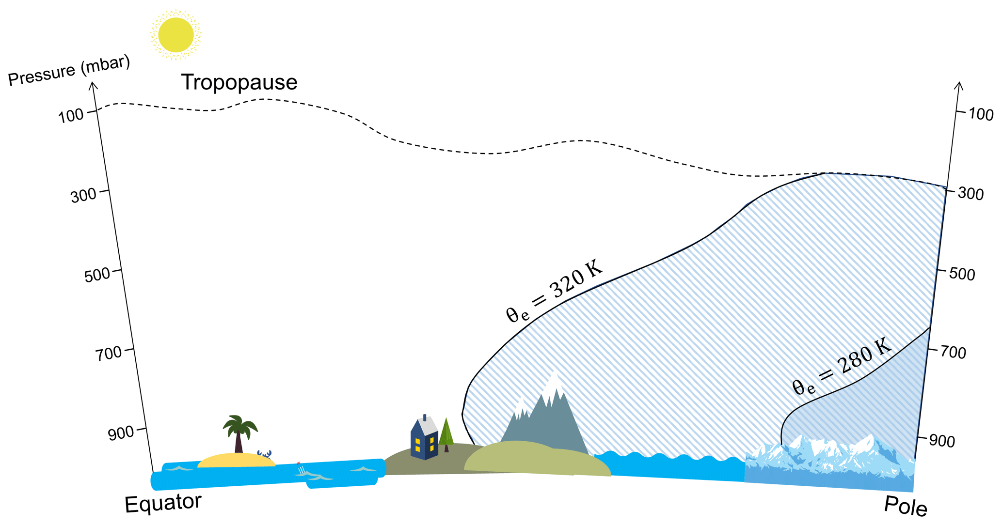
Figure 1Schematic of the conceptual basis to calculate . of a given θe surface is computed by summing all dry air mass with a low equivalent potential temperature in the troposphere of the hemisphere. This calculation yields a unique θe– relation at a given time point.
This calculation yields a unique value of for each value of θe. We refer to the relationship between θe and as the “θe– look-up table”, which we generate at daily resolution. We provide this look-up table for each hemisphere computed from ERA-Interim from 1980 to 2018 with a daily resolution and from the lowest to the highest θe surface in the troposphere with 1 K intervals (see data availability).
3.1 Spatial and temporal distribution of
Figure 2 shows snapshots of the distribution of zonal average θe and with latitude and pressure at two arbitrary time slices (1 January 2009, 1 July 2009). is not continuous across the Equator because it is defined separately in each hemisphere. By definition, each surface is exactly aligned with a corresponding θe surface, and surfaces have the same characteristics as θe surfaces, which decrease with latitude and generally increase with altitude. Whereas the zonal average θe surfaces vary by up to 20∘ in latitude over seasons, the meridional displacement of zonal average is much smaller, with less than 5∘ in latitude poleward of 30∘ N and S, as expected, because the zonal average displacement of atmospheric mass over seasons is small. This small seasonal displacement is closely associated with the seasonality of vertical sloping of θe surfaces (Fig. 2). As the mass under each surface is always constant, the change in tilt must cause the meridional displacement. In the summer, the tilt is steeper (due to increased deep convection), so surfaces move poleward in the lower troposphere but move equatorward in the upper troposphere.
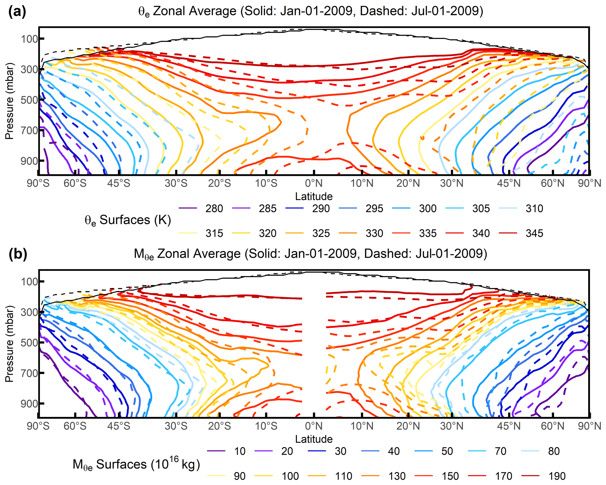
Figure 2Snapshot of the distribution of (a) zonal average θe surfaces on 1 January 2009 (solid lines) and 1 July 2009 (dashed lines) and (b) zonal average surfaces on 1 January 2009 (solid lines) and 1 July 2009 (dashed lines). The zonal average tropopause is also shown here for 1 January 2009 (solid black line) and 1 July 2009 (dashed black line). θe, , and the tropopause are computed from ERA-Interim.
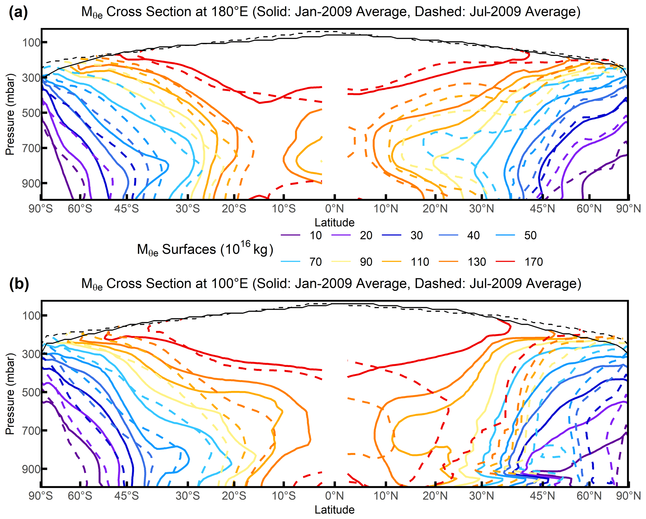
Figure 3 surfaces as January 2009 average (solid lines) and July 2009 average (dashed lines) for (a) 180∘ E (mostly over the Pacific Ocean), and (b) 100∘ E (mostly over the Eurasia land in the Northern Hemisphere). and the tropopause are computed from ERA-Interim.
surfaces at given meridians (Fig. 3) in the Northern Hemisphere show clear zonal asymmetry, with larger and more complex displacements compared to the zonal averages, associated with differential heating by land and ocean and orographic stationary Rossby waves (Hoskins and Karoly, 1981; Wills and Schneider, 2018). For example, over the Northern Hemisphere ocean at 180∘ E (Fig. 3a) and from the summer to winter, surfaces move poleward in the middle to high latitudes (e.g., poleward of 45∘ N) but move equatorward in the mid- to low-latitude lower troposphere (e.g., equatorward of 45∘ N, 900–700 mbar), with the magnitude smaller than 10∘ latitude in both. In comparison, over the Northern Hemisphere land at 100∘ E (Fig. 3b) and from the summer to winter, surfaces move equatorward by up to 30∘ latitude, except in the high-latitude middle troposphere (e.g., poleward of 70∘ N, ∼ 500 mbar), where the flat surfaces lead to slightly poleward displacements. In the Southern Hemisphere, in contrast, the summer-to-winter displacements of the 180 and 100∘ E sections are similar to the zonal average.
At lower latitudes, the zonal averages of and θe both exhibit strong secondary maxima near the surface associated with the Hadley circulation (equatorward of 30∘ N and S) and in the summer, driven by high water vapor. From the contours in Fig. 2, this surface branch of high and θe appears disconnected from the upper tropospheric branch. In fact, these two branches are connected through air columns undergoing deep convection, which are not resolved in the zonal means shown in Fig. 2 but are resolved in some meridians (e.g., Fig. 3a). We also note that, over the land at 100∘ E (Fig. 3b), the two disconnected and θe branches in the Northern Hemisphere summer are displaced poleward compared to the zonal average, consistent with a northward shift of the intertropical convergence zone (ITCZ) over southern Asia. The existence of these two branches may limit some applications of , as discussed in Sect. 4.
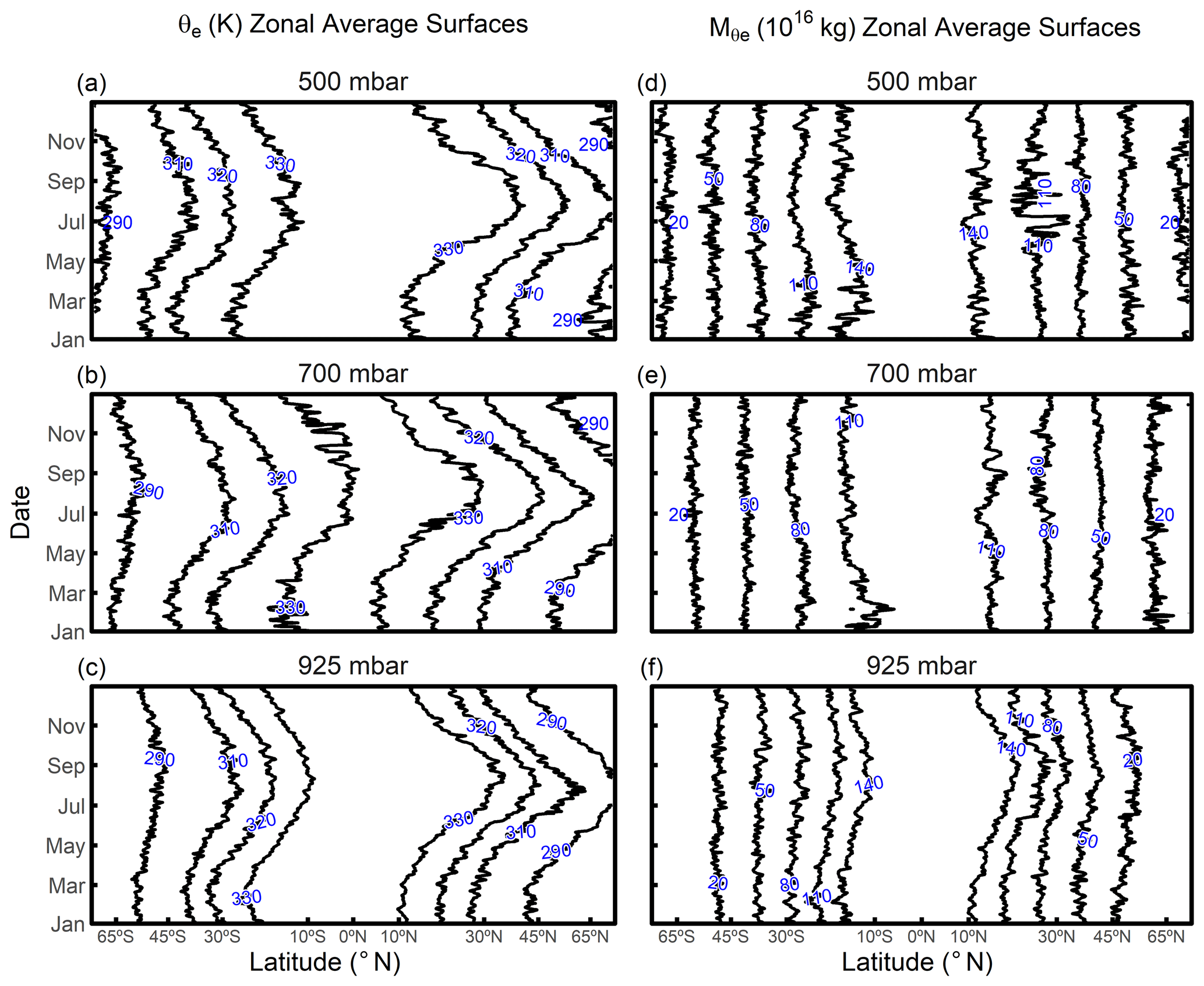
Figure 4Time series of meridional displacement of selected zonal average θe (K) surfaces over a year at (a) 500 mbar, (b) 700 mbar, and (c) 925 mbar. Meridional displacement of selected zonal average (1016 kg) surfaces over a year at (d) 500 mbar, (e) 700 mbar, and (f) 925 mbar. The value of each surface is labeled. θe and are computed from ERA-Interim. Results shown are for the year 2009.
Figure 4 shows the zonal average meridional displacement of θe and with a daily resolution. In summer, surfaces displace poleward in the lower troposphere but equatorward in the upper troposphere. The displacements in the lower troposphere (925 mbar) are greater in the Northern Hemisphere, where the kg surface, for example, displaces poleward by 10∘ in latitude between winter and summer (Fig. 4b). Beside the seasonal variability, Fig. 4 also shows evident synoptic-scale variability.
Since the tilting of θe surfaces has an impact on the seasonal displacement of surfaces, the contribution of different pressure levels to the mass of a given bin must also vary with season. In Fig. 5, we show these contributions as two daily snapshots on 1 January and 1 July 2009. Low bins consist of air masses mostly below 500 mbar near the pole. As increases, the contribution from the upper troposphere gradually increases while the contribution from the surface to 800 mbar decreases to its minimum at around 100 × 1016 to 120 × 1016 kg. The contribution from the surface to 800 mbar increases as increases above 120 × 1016 kg. The mass fraction shows only small variations with season, with the lower troposphere (surface to 800 mbar) contributing slightly less in the low- bands and slightly more in the high- bands in the summer, which is closely related to the seasonal tilting of corresponding θe surfaces.
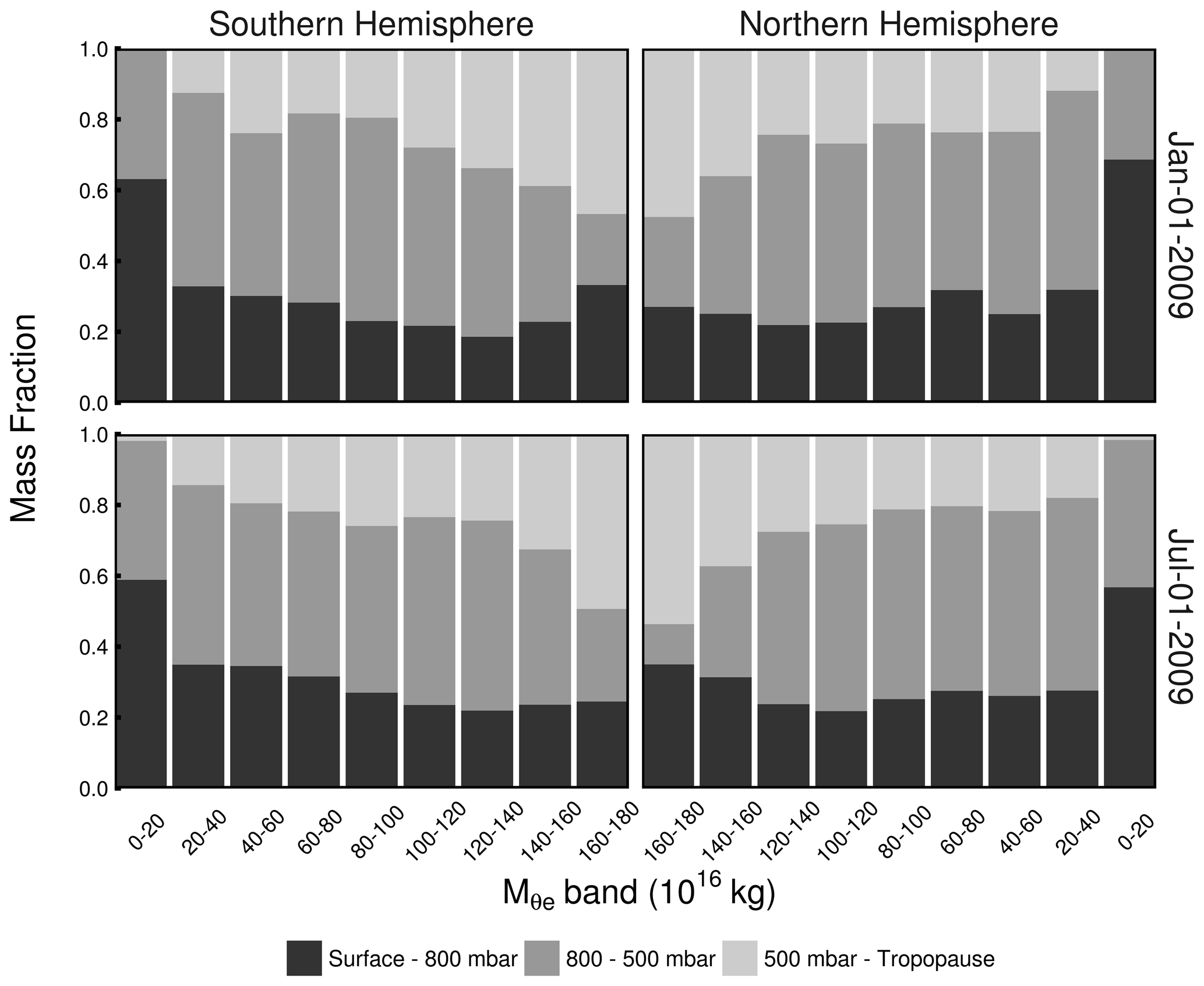
Figure 5Snapshots (1 January 2009 and 1 July 2009) of the mass distribution of different bins from three pressure bins (surface to 800 mbar, 800 to 500 mbar, and 500 mbar to tropopause). is computed from ERA-Interim. Low bins are seen to have larger contributions from the air near the surface, and high bins have larger contributions from air aloft. Comparing the top and the bottom panels shows that the seasonal differences in pressure contributions are small except for the highest bins (160 × 1016–180 × 1016 kg) and the lowest bin in the Northern Hemisphere (0–20 × 1016 kg).
3.2 θe– relationship
Figure 6 compares the temporal variation in of several given θe surfaces (i.e., θe– look-up table) computed from different reanalysis products for 2009. The deviations are indistinguishable between ERA-Interim and MERRA-2, except near θe=340 K, where MERRA-2 is systematically lower than ERA-Interim by 1.5 × 10¹⁶ to 6.5 × 10¹⁶ kg. NCEP2 shows slightly larger deviations from ERA-Interim but by less than 8.5 × 10¹⁶ kg. The products are highly consistent in seasonal variability, and they also show agreement on synoptic timescales. The small difference between products is expected because of different resolutions and methods (Mooney et al., 2011). We expect these differences would be negligible for most applications of .
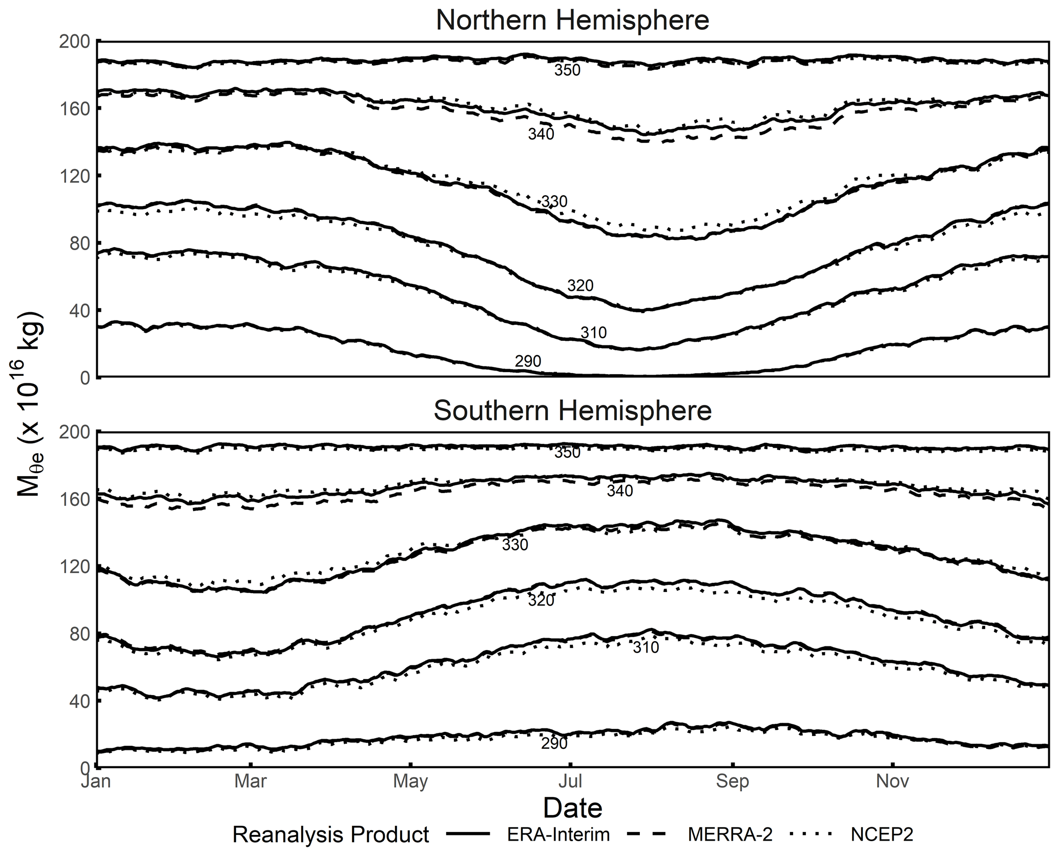
Figure 6Variability in of given θe surfaces (i.e., θe– look-up table) over a year with a daily resolution in the Northern and Southern Hemisphere. Data from ERA-Interim are shown as a solid line; MERRA-2 data are shown as a dashed line, and NCEP2 data are shown as a dotted line. Results shown are for the year 2009.
Figure 6 shows that, in both hemispheres, reaches its minimum in summer and maximum in winter for a given θe surface, with the largest seasonality at the lowest θe (or ) values. The seasonality decreases as θe increases, following the reduction in the seasonality of shortwave absorption at lower latitudes (Li and Leighton, 1993). The seasonality is smaller in the Southern Hemisphere, consistent with the larger ocean area and hence greater heat capacity and transport (Fasullo and Trenberth, 2008; Foltz and McPhaden, 2006). Figure 6 also shows that has significant synoptic-scale variability although smaller than the seasonal variability. Synoptic variability is typically larger in winter than summer, as discussed below.
3.3 Relationship to diabatic heating and mass fluxes
A key step of the application of for interpreting tracer data is the generation of the look-up table that relates θe and . In this section, we address a tangential question of what controls the temporal variation in the look-up table, which is not necessary for the application but may be of fundamental meteorological interest.
As shown in Appendix A, the temporal variation in the look-up table, , can be related to underlying mass and heat fluxes according to
where (J s−1 K−1) is the effective diabatic heating, integrated over the full θe surface per unit width in θe; mT(θet) (kg s−1) is the net mass flux across the tropopause; and mE(θet) (kg s−1) is the net mass flux across the Equator, including all air with equivalent potential temperature of less than θe. Qdia has contributions from internal heating without ice formation (), heating from ice formation (Qice), sensible heating from the surface (Qsen), surface evaporation (Qevap), turbulent diffusion of heat (Qdiff), and turbulent transport of water vapor () following
The terms Qevap and are expressed as heating rates by multiplying the underlying water fluxes by Lv(T)∕Cpd. In order to quantify the dominant processes contributing to temporal variation in , the terms in Eqs. (8) and (9) must be linked to diagnostic variables available in the reanalysis or model products. Although there was no perfect match with any of the three reanalysis products, MERRA-2 provides temperature tendencies for individual processes, which can be converted to heating rates per Eq. 9 following
where i refers to a specific process (, Qice, etc.), (K s−1) is the temperature tendency of grid cell x, Mx (kg) is the mass of grid cell x, and Δθe is the width of the θe surface.
Table 1Correspondence of heating variables between our derivation (Eq. 9) and MERRA-2.
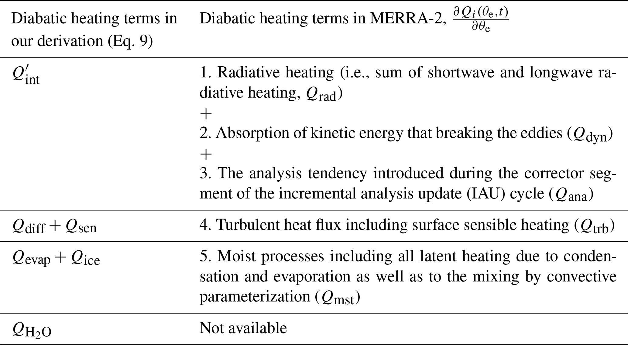
There are five heating terms provided in the MERRA-2 product, which we can approximately relate to terms in Eq. (9), as shown in Table 1. The first three terms (Qrad, Qdyn, and Qana) can be summed to yield ; the fourth (Qtrb) is equal to the sum of Qdiff and Qsen; and the fifth (Qmst) approximates the sum of Qice and Qevap. MERRA-2 does not provide terms corresponding to or Qevap, but Qmst represents heating due to moist processes, which includes Qice plus water vapor evaporation and condensation within the atmosphere. This water vapor evaporation and condensation should be approximately equal to Qevap with a small time lag when integrated over a θe surface because mixing is preferentially along θe surfaces and water vapor released into a θe surface by surface evaporation will tend to transport and precipitate from the same θe surface within a short time period (Bailey et al., 2019). Thus, the MERRA-2 term for heating by moist processes (Qmst) should approximate Qice+Qevap.
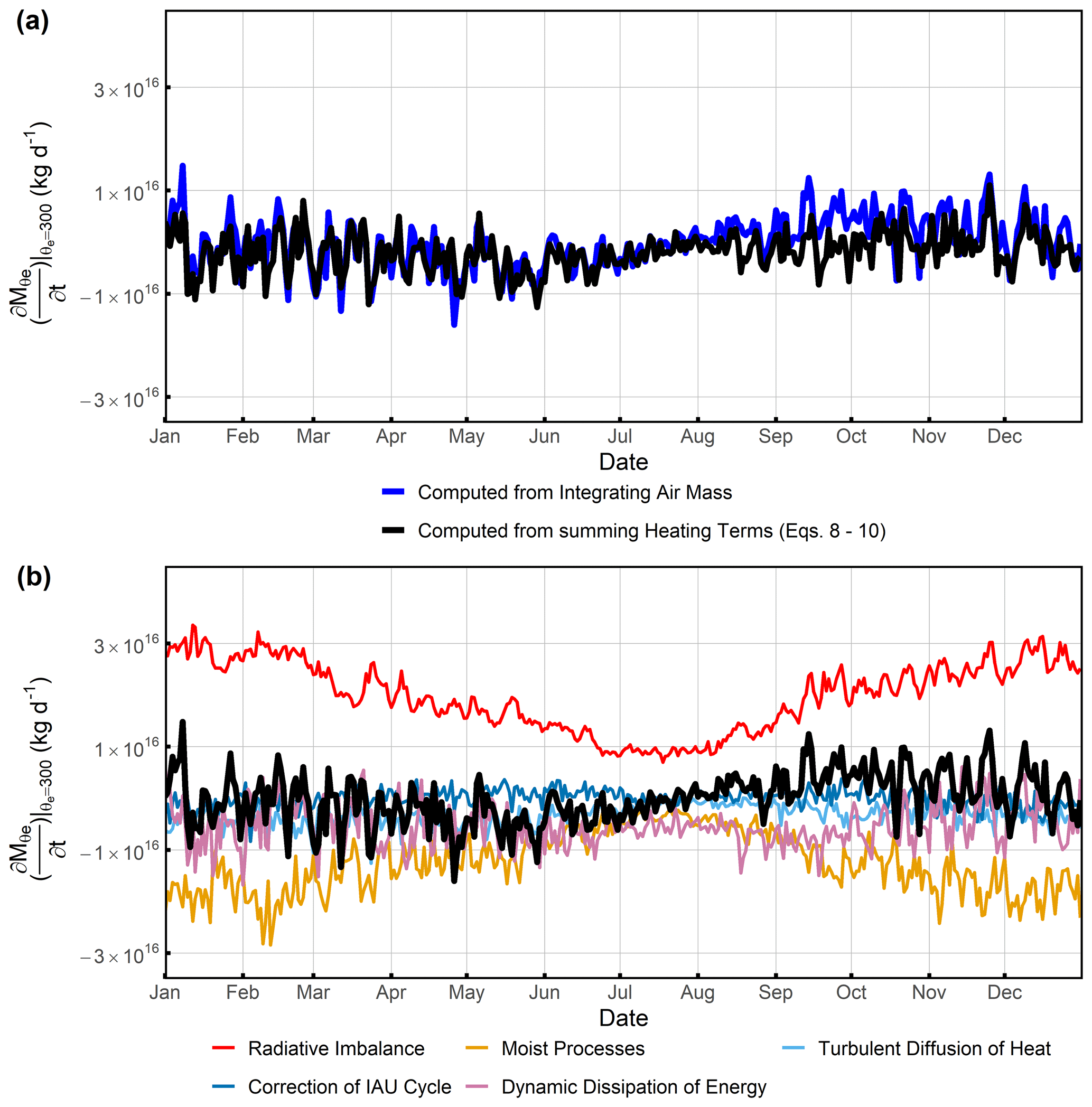
Figure 7(a) Temporal variation in in the Northern Hemisphere at θe=300 K computed by integrating air mass (blue line) and estimated from the sum of five heating terms (Table 1) in MERRA-2 (black line). (b) The heating variables are decomposed into five contributions as indicated (see Table 1). Results shown are for the year 2009.
Figure 7a compares the temporal variation in computed by integrating the dry air mass (i.e., θe– look-up table) with computed from the sum of the diabatic heating terms from MERRA-2 (via Eqs. 8 to 10). The comparison focuses on the θe=300 K surface, which does not intersect with the Equator or tropopause, so the two mass flux terms (mT, mE) vanish. These two methods have a high correlation at 0.71. We do not expect perfect agreement because computed by the sum of heating neglects turbulent water vapor transport (), and only approximates Qevap as discussed above. This relatively good agreement nevertheless demonstrates that the formulation based on MERRA-2 heating terms includes the dominant processes that drive temporal variations in the look-up table. Figure 7a shows poorer agreement from late August to October, which we also find in other years (Figs. S1 and S2 in the Supplement) and on lower (e.g., θe=290 K, Fig. S3) but not higher (e.g., θe=310 K, Fig. S4) surfaces, where the two methods agree better. The poor agreement may reflect a partial breakdown of the assumption that Qmst approximates the sum of Qice and Qevap, but further analysis is beyond the scope of this study.
Figure 7b further breaks down the sum of the heating terms in Eqs. (8) and (10) from MERRA-2 into individual components. Each term clearly displays variability on synoptic to seasonal scales. To quantify the contribution of different terms on the different timescales, we separate each term into a seasonal and synoptic component, where the seasonal component is derived by a two-harmonic fit with a constant offset and the synoptic component is the residual. We estimate the fractional contribution of each heating term on seasonal and synoptic timescales separately in Table 2, using the method in Sect. S1 in the Supplement. On the seasonal timescale, the variance is dominated by radiative heating and cooling of the atmosphere and moist processes (including both ice formation and extra water vapor from surface evaporation) together, with prominent counteraction between them. On the synoptic timescale, dissipation of the kinetic energy of turbulence dominates the variance.
Table 2Fractional contribution of the individual heating terms in Fig. 7b to their sum for θe=300 K. The analysis is done separately on synoptic and seasonal components. The seasonal component is based on a two-harmonic fit, and the synoptic component is defined as the residual. The fractional contributions sum to 1, while a positive contribution means in phase and negative contribution means anti-phase. A contribution of an absolute value that is bigger than 1 illustrates that the variability in the heating term is larger than the variability in the sum on the corresponding timescale.

Similar analyses on different θe surfaces and in different years (Figs. S1 to S4) all show that a combination of radiative heating and moist processes dominates the temporal variation in on the seasonal timescale, while dissipation of the kinetic energy of turbulence dominates on the synoptic timescale.
To illustrate the potential application of for interpreting sparse data, we focus on the seasonal cycle of CO2 in the Northern Hemisphere as resolved by two series of global airborne campaigns, HIPPO and ATom. HIPPO consisted of five campaigns between 2009 and 2011, and ATom consisted of four campaigns between 2016 and 2018. Each campaign covered from ∼ 150 to ∼ 14 000 m and from nearly pole to pole, along both northbound and southbound transects. On HIPPO, both transects were over the Pacific Ocean, while on ATom, southbound transects were over the Pacific Ocean and northbound transects were over the Atlantic Ocean. The flight tracks are shown in Fig. 8a. We aggregate data from each campaign into northbound and southbound transects within each hemisphere but only use data from the Northern Hemisphere. We only consider tropospheric observations by excluding measurements from the stratosphere, which is defined by observed water vapor of less than 50 ppm and either O3 greater than 150 ppb or detrended N2O to the reference year of 2009 of less than 319 ppb. Water vapor and O3 were measured by the NOAA UCATS (Unmanned Aerial Systems Chromatograph for Atmospheric Trace Species; Hurst, 2011) instrument and were interpolated to a 10 s resolution. N2O was measured by the Harvard QCLS (Quantum Cascade Laser System; Santoni et al., 2014) instrument. Furthermore, we exclude all near-surface observations within ∼ 100 s of takeoffs and within ∼ 600 s of landings as well as missed approaches, which usually show high CO2 variability due to strong local influences. In situ measurements of CO2 were made by three different instruments on both HIPPO and Atom. Of these, we use the CO2 measurements made by the NCAR Airborne Oxygen Instrument (AO2) with a 2.5 s measurement interval (Stephens et al., 2020), for consistency with planned future applications of APO (atmospheric potential oxygen) computed from AO2. The differences between instruments are small for our application (Santoni et al., 2014). The data used in this study are averaged to a 10 s resolution, and we show the detrended CO2 values along each airborne campaign transect for the Northern Hemisphere in Fig. 8b. Since we focus on the seasonal cycle of CO2, all airborne observations are detrended by subtracting an interannual trend fitted to CO2 measured at the Mauna Loa Observatory (MLO) by the Scripps CO2 Program. This trend is computed by a stiff cubic spline function plus four-harmonic terms with linear gain to the MLO record. is computed from ERA-Interim in this section.
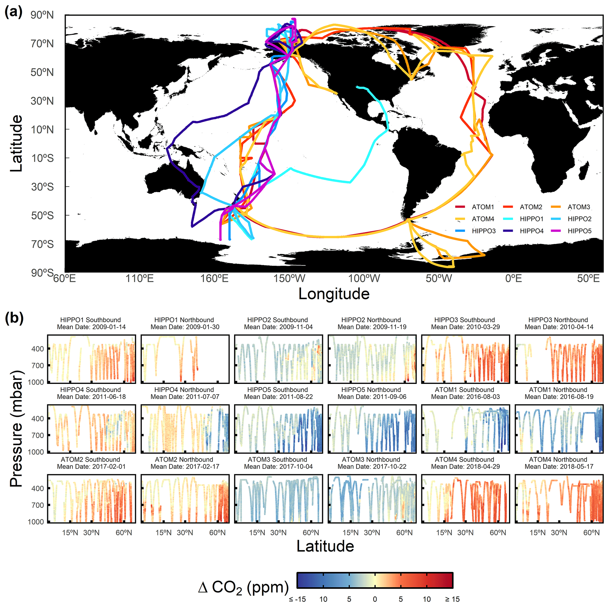
Figure 8(a) HIPPO and ATom horizontal flight tracks colored by campaigns. (b) Latitude and pressure cross section of detrended CO2 of each airborne campaign transect. CO2 is detrended by subtracting the MLO stiff cubic spline trend, which is computed by a stiff cubic spline function plus four-harmonic functions with linear gain to the MLO record.
4.1 Mapping Northern Hemisphere CO2
A conventional method to display seasonal variations in CO2 from airborne data is to plot time series of the data at a given location or latitude and different pressure levels (Graven et al., 2013; Sweeney et al., 2015). In Fig. 9, we compare this method using HIPPO and ATom airborne data, binning and averaging the data from each airborne campaign transect by pressure and latitude bins, with our new method, binning the data by pressure and . For each latitude bin, we choose a corresponding bin which has approximately the same meridional coverage in the lower troposphere. We remind the reader that decreases poleward while also generally increasing with altitude (Figs. 2 to 4).
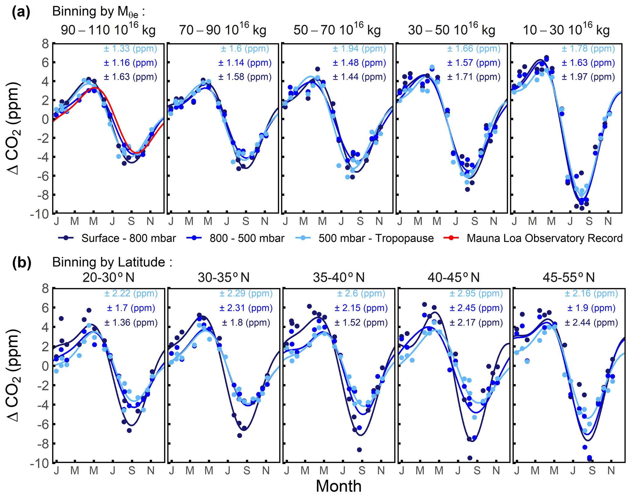
Figure 9Seasonal cycles of airborne Northern Hemisphere CO2 data sorted by (a) –pressure bins and (b) latitude–pressure bins. bins (1016 kg) and latitude bins are shown at the top of each panel. Pressure bins are colored. The latitude bounds are chosen to approximate the meridional coverage of each corresponding bin in the lower troposphere. The seasonal cycle at MLO from 2009 to 2018 is shown in the 90–110 bin panel, which spans the of the station. Airborne observations are first grouped into –pressure or latitude–pressure bins and then averaged for each airborne campaign transect, shown as points. We filter out the points averaged from fewer than twenty 10 s observations. The seasonal cycle of airborne data and MLO (2009–2018) are computed by a two-harmonic fit to the detrended time series. The 1σ variability about the seasonal cycle fits for each –pressure or latitude–pressure bin is labeled at the top of each panel. These 1σ values are based on the distribution of all binned observations (not shown), rather than on the distribution of average CO2 of each bin and airborne campaign transect (shown).
As shown in Fig. 9, the transect averages of detrended CO2 (shown as points) from both binning methods resolve well-defined seasonal cycles (based on two-harmonic fit) in all bins, with higher amplitudes near the surface (low pressure) and at high latitudes (low ). However, binning by leads to much smaller variations in the mean seasonal cycle (shown as solid curves) with pressure, as expected, because moist isentropes are preferential surfaces for mixing. Also, within individual pressure bins, the short-term variability relative to the mean cycles based on the distribution of all detrended observations (not shown as points but denoted as 1σ values in Fig. 9) is smaller when binning by (F test, p < 0.01), except in the lower troposphere of the highest bin (90 × 1016–110 × 1016 kg). The smaller short-term variability is expected because tracks the synoptic variability in the atmosphere. When binning by latitude, the smallest short-term variability is found at the lowest bin (surface–800 mbar) and the largest short-term variability is found in the highest bin (500 mbar tropopause), except the highest latitude bin (45–55∘ N). When binning by , in contrast, the short-term variability in the middle pressure bin is always smaller than the higher and lower pressure bins (F test, p < 0.01), except for the 50-to-70 bin, where the difference between the lowest and middle pressure bins is not significant (based on 1σ levels). The lower variability in the middle troposphere may reflect the suppression of variability from synoptic disturbances, leaving a clearer signal of the influence of surface fluxes of CO2 and stratosphere–troposphere exchanges. We compare the variance of detrended airborne observations within each –pressure bin with its fitted value. The fitted seasonal cycle of each bin explains 63.2 % to 90.5 % of the variability for different bins, with higher fractions in the middle troposphere.
Figure 9 also shows the CO2 seasonal cycle at MLO, which falls within a single –pressure bin (90 × 1016–110 × 1016 kg, 500–800 mbar) at all seasons. Although the airborne data in this bin span a wide range of latitudes (∼ 10–75∘ N), the seasonal cycle averaged over this bin is very similar to the cycle at MLO (airborne cycle leads by ∼ 10 d with 1.0 % lower amplitude). This small difference is within the 1σ uncertainty in our estimation from airborne observation, and some difference is expected, since we choose a –pressure bin wider than the seasonal variation in and pressure at MLO.
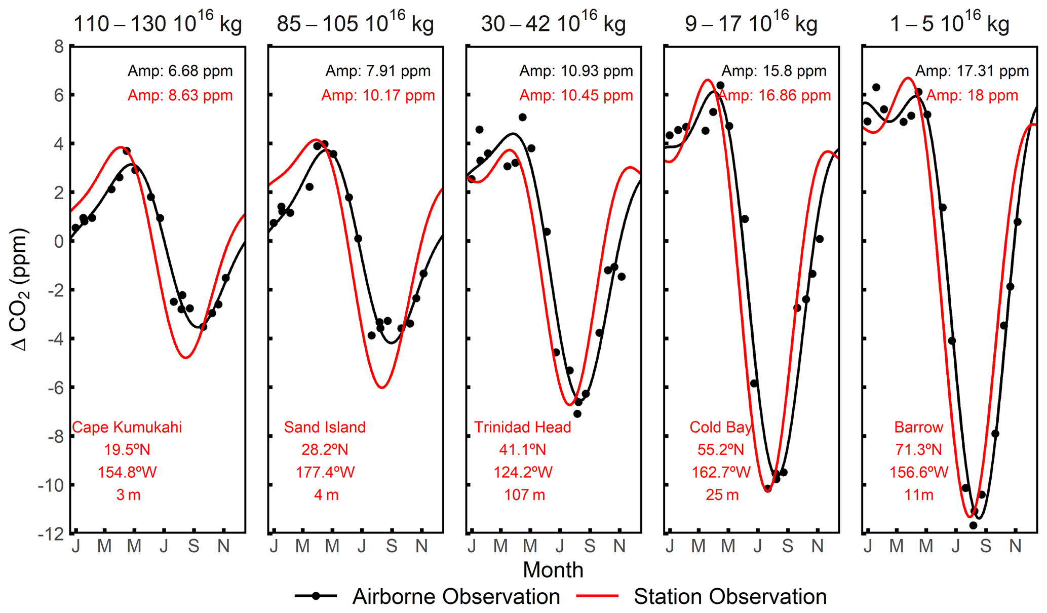
Figure 10CO2 seasonal cycles of multiple surface stations (2009–2018) compared to seasonal cycles of airborne observations averaged over corresponding bin. The choice of bin is to approximate the range of at each corresponding surface station and is shown at the top of each panel. Daily of the station is computed from ERA-Interim, based on its location. We detrend station and airborne observations by subtracting the MLO stiff cubic spline trend. We compute average detrended CO2 for each airborne campaign transect and each bin, shown as black points. The seasonal cycles are computed from a two-harmonic fit, with the seasonal amplitude (Amp) shown in the upper right of each panel.
It is also of interest to examine how CO2 data from surface stations fit into the framework based on . Figure 10 compares the CO2 seasonal cycle of five NOAA surface stations (Cooperative Global Atmospheric Data Integration Project, 2019) with the cycle from the airborne observations binned into selected bins. These surface stations are chosen to be representative of different ranges. For the comparison, we chose bins that span the seasonal maximum and minimum value of the station. These bins are narrower than the bins used in Fig. 9, in order to sharply focus on the latitude of the station. To maximize sampling coverage, we bin the airborne data only by without pressure sub-bins. For mid- and high-latitude surface stations (right three panels), the seasonal amplitude of station CO2 and corresponding airborne CO2 are close (within 4 %–5 %), while airborne cycles lag by 2–3 weeks. The lag presumably represents the slow mixing from the mid-latitude surface to the high-latitude mid-troposphere (Jacob, 1999). In contrast, for low-latitude stations (left two panels) which generally sample trade winds, the seasonal cycles differ significantly, indicating that the air sampled at these stations is not rapidly mixed along surfaces of constant or θe with air aloft. As mentioned above (Sect. 3.1), surfaces of high within the Hadley circulation have two branches, one near the surface and one aloft. A timescale of several months for transport from the lower to the upper branch can be estimated from the known overturning flows based on air mass flux stream functions (Dima and Wallace, 2003). This delay, plus strong mixing and diabatic effects (Miyazaki et al., 2008), ensures that the lower and upper branches are not well connected on seasonal timescales. Our results nevertheless demonstrate that the framework combining airborne and surface data could help understanding of details of atmospheric transport both along and across θe surfaces.
4.2 Computing the hemispheric mass-weighted average CO2 mole fraction
We next illustrate the use of for computing the mass-weighted average of a long-lived chemical tracer by performing this exercise for CO2 in the Northern Hemisphere. We calculate the Northern Hemisphere tropospheric mass-weighted average CO2 from each airborne transect using a method that assumes that CO2 is uniformly mixed on θe surfaces throughout the hemisphere (Barnes et al., 2016; Parazoo et al., 2011, 2012). We exclude airborne observation from HIPPO-1 Northbound due to the lack of data north of 40∘ N. We use the θe– look-up table of the corresponding date to assign a value of to each observation based on its θe. The observations for each transect are then sorted by . The hemispheric average CO2 is calculated by trapezoidal integration of CO2 as a function of and divided by the total dry air mass as computed from the corresponding range of .
To illustrate the integration method, we choose HIPPO-1 Southbound and show CO2 measurements and ΔCO2 atmospheric inventory (Pg) as a function of in Fig. 11. The Northern Hemisphere tropospheric average detrended ΔCO2 is computed by integrating the area under the curve (subtracting negative contributions) and dividing by the maximum value of within the hemisphere (here 195.13 × 10¹⁶ kg). This yields a mass-weighted average detrended ΔCO2 of 1.13 ppm for the full troposphere of the Northern Hemisphere. The trapezoidal integration has a high accuracy because the data are dense over . The ΔCO2 atmospheric inventory is dominated by the domain < 120 ×1016 kg (mid-latitude to high latitude), which has a large CO2 seasonal cycle driven by a temperate and boreal ecosystem, with less than 4.1 % contributed by the additional ∼ 38.8 % of the air mass outside this domain in the low latitudes or upper troposphere (Fig. 11b), where ΔCO2 differs less from the subtracted baseline.
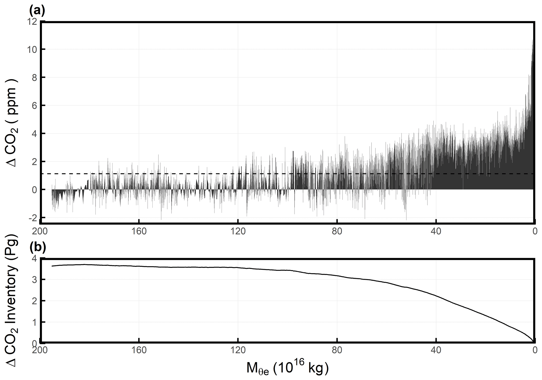
Figure 11(a) Detrended CO2 measurements from HIPPO-1 Southbound (from 12 to 17 January 2009) plotted as a function of in the Northern Hemisphere. The data are detrended by subtracting the MLO stiff cubic spline trend. Individual points are connected by straight line segments, and the area under the resulting curve is shaded. We note that the area under the curve has units of parts per million × kilograms, and dividing this by the total dry air mass (i.e., the range of of the integral) gives the parts per million unit because the mass of dry air is proportional to the moles of dry air. The Northern Hemisphere average of 1.13 ppm is indicated by the dashed line. (b) Integral of the data in panel (a), rescaled from parts per million to petagrams, integrating from to a given value.
We compute Northern Hemisphere mass-weighted average detrended ΔCO2 for each airborne campaign transect and fit the time series to a two-harmonic fit to estimate the seasonal cycle (Fig. 12). We find that the cycle has a seasonal amplitude of 7.9 ppm and a downward zero-crossing on Julian day 179, where the latter is defined as the date when the detrended seasonal cycle changes from positive to negative.
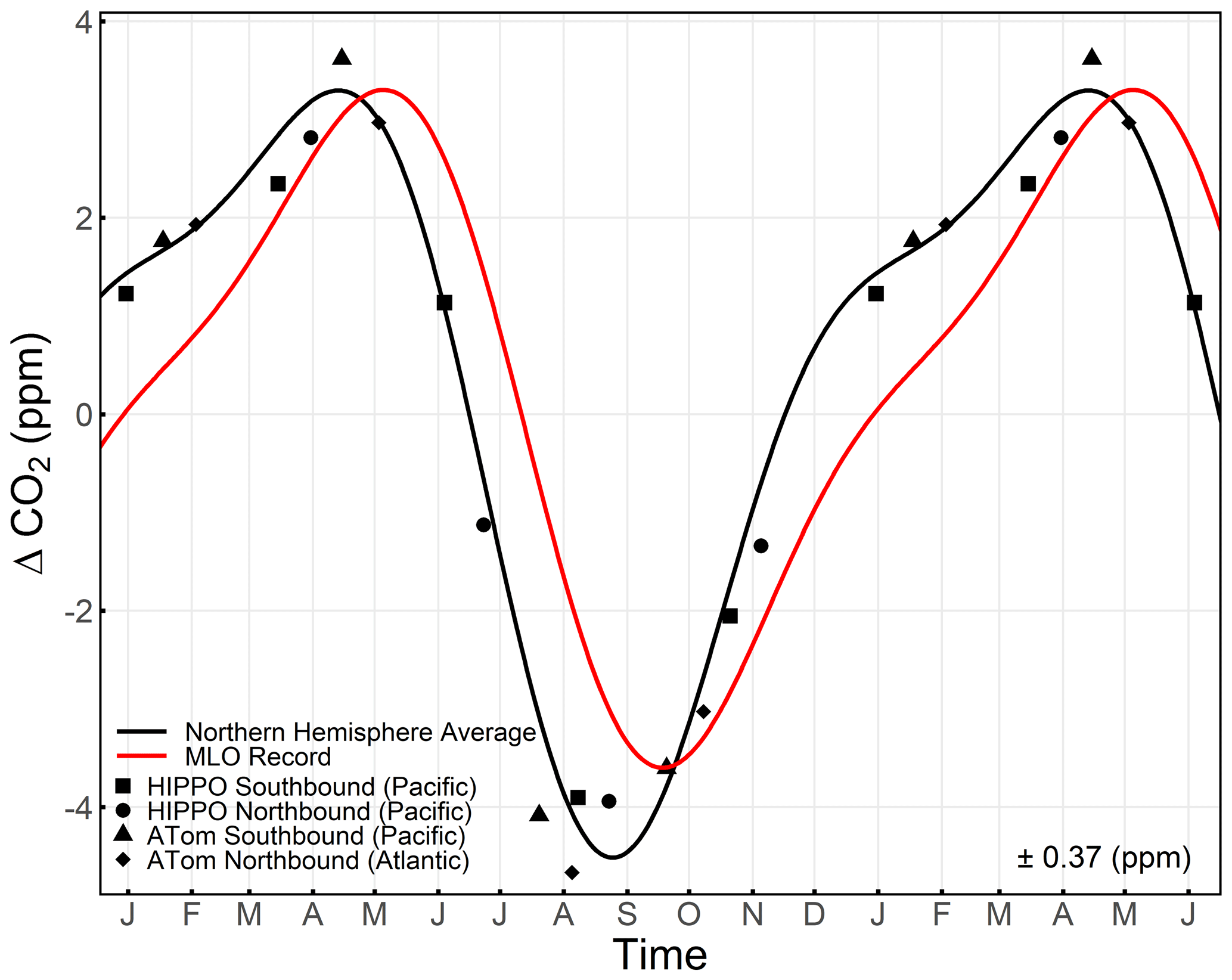
Figure 12Comparison between the CO2 seasonal cycle of Northern Hemisphere tropospheric average computed from airborne observation and the integration method (black points and line) and the mean cycle at MLO measured by Scripps CO2 Program from 2009 to 2018 (red line). Both are detrended by subtracting a stiff cubic spline trend at MLO. We then compute mass-weighted average detrended CO2 for each airborne campaign transect, shown as black points, with campaigns and transects presented as different shapes. The seasonal cycle of both are computed by a two-harmonic fit to the detrended time series. The 1σ variability in the detrended average CO2 values about the fit line is shown on the lower right. The first half year is repeated for clarity.
To address the error in our estimation of the Northern Hemisphere mass-weighted average CO2 seasonal cycle from HIPPO and Atom airborne observation, we consider two main sources: (1) irreproducibility in the CO2 measurements and (2) limited coverage in space and time. For the first contribution, we compute the difference between mass-weighted average CO2 from AO2 and mean mass-weighted average CO2 from Harvard QCLS, Harvard OMS, and NOAA Picarro for each airborne campaign transect, while masking values that are missing in any of these datasets. We compute the standard deviation of these differences (±0.15 ppm) for the mass-weighted average CO2 of each airborne campaign transect as the 1σ level of uncertainty. We further compute the uncertainties for the seasonal amplitude of ±0.11 ppm and for the downward zero-crossing of ±0.83 d, which are calculated from 1000 iterations of the two-harmonic fit, allowing for random Gaussian uncertainty (σ 0.15 ppm) for each transect.
Table 3RMSE, seasonal amplitude, and day of year of the downward zero-crossing of each simulation based on the Jena CO2 inversion. The true value (daily average CO2) is computed by integrating over all tropospheric grid cells of the Jena CO2 inversion, while troposphere is defined by PVU < 2 from ERA-Interim. Seasonal amplitude and downward zero-crossing of true average and each simulation is computed from two-harmonic fit to the detrended value, which is detrended by subtracting the MLO cubic stiff spline. Subsampling with randomly retaining a certain fraction of data are conducted by randomly subsampling 1000 times, thus, the seasonal amplitude and day of year of the downward zero-crossing is computed as the mean ± standard deviation of the 1000 iterations.
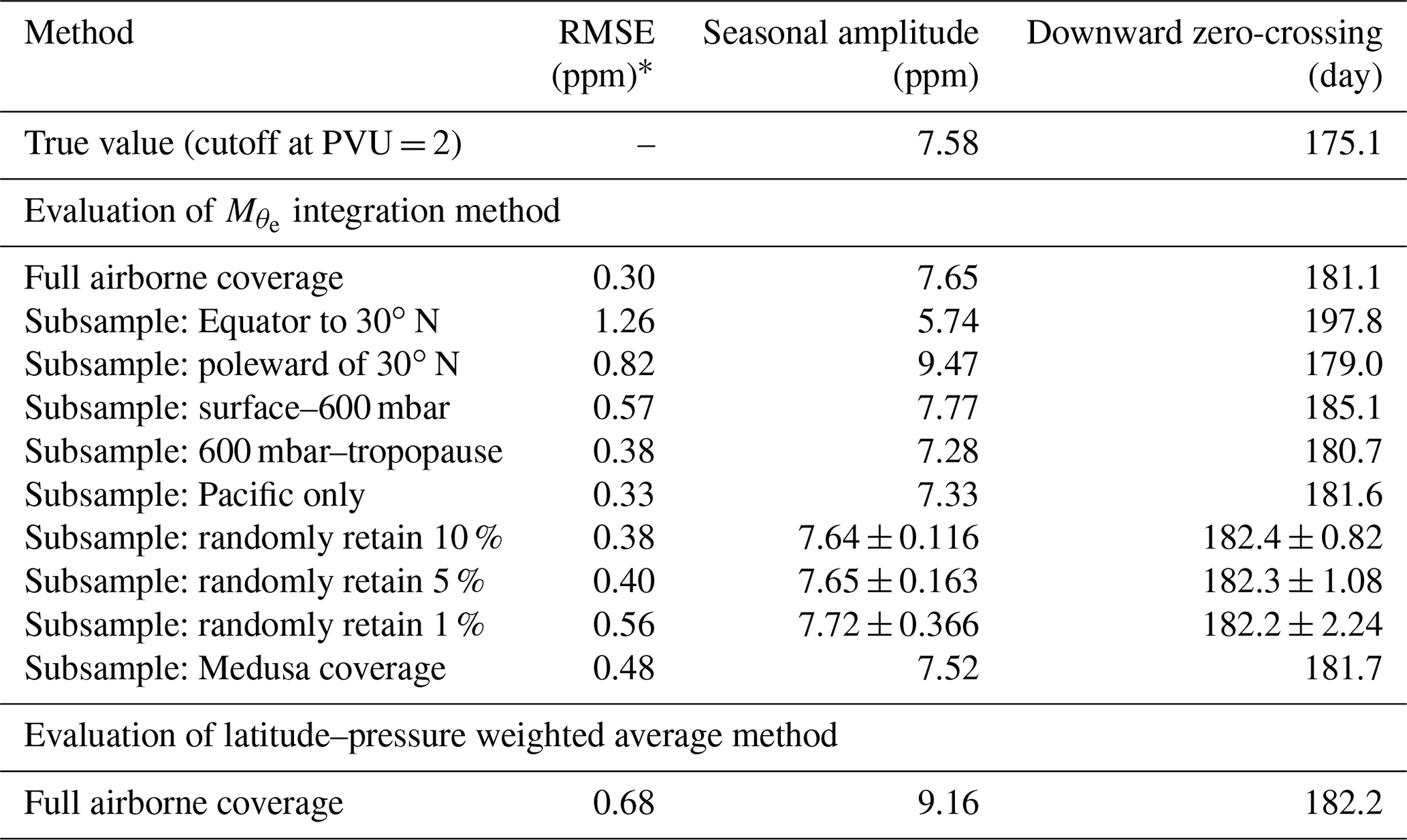
∗ Each simulation yields 17 data points of different dates over the seasonal cycle from 17 airborne campaign transects. RMSE of each simulation is computed with respect to the true value.
For the contribution to the error in the amplitude and phase from limited special and temporal coverage, we use simulated CO2 data from the Jena CO2 inversion Run ID s04oc v4.3 (Rödenbeck et al., 2003). This model includes full atmospheric fields from 2009 to 2018, which we detrend using the cubic spline fit to the observed MLO trend. From these detrended fields, we compute the climatological cycle of the Northern Hemisphere average by integrating over all tropospheric grid cells (cutoff at PVU = 2) to produce a daily time series of the hemispheric mean, which we take as the model “truth”. We fit a two-harmonic function to this true time series to compute a true climatological cycle over the 2009–2018 period (Table 3), which is our target for validation. We then subsample the Jena CO2 inversion along the HIPPO and ATom flight tracks and process the data similarly to the observations, using the integration method and a two-harmonic fit. The comparison shows that the integration method yields an amplitude which is 1 % too large and yields a downward zero-crossing date which is 6 d too late. We view these offsets as systematic biases, which we correct from the observed amplitude and phase reported above. The uncertainties in these biases are hard to quantify, but we take ±100 % as a conservative estimate. We thus allow an additional random error of ±0.08 ppm in amplitude and ±6.0 d in downward zero-crossing for uncertainty in the bias. Combining the random and systematic error contributions leads to a corrected Northern Hemisphere tropospheric average CO2 seasonal cycle amplitude of 7.8 ± 0.14 ppm and downward zero-crossing of 173 ± 6.1 d. This corrected cycle is an estimate of the climatological average from 2009 to 2018.
The error due to limited spatial and temporal coverage can be divided into three components: limited seasonal coverage (17 transects over the climatological year), limited interannual coverage (sampling particular years instead of all years), and limited spatial coverage (under-sampling the full hemisphere). We quantify the combined biases due to both limited seasonal and limited interannual coverage by comparing the two-harmonic fit of the full true daily time series of the hemispheric mean to a two-harmonic fit of those data subsampled on the actual mean sampling dates of the 17 flight tracks. We isolate the bias associated with limited seasonal coverage by repeating this calculation, replacing the true daily time series with the daily climatological cycle. The bias associated with limited spatial coverage is quantified as the residual. Combining these results, we estimate that the limited seasonal, interannual, and spatial coverage account for biases in the downward zero-crossing of 1.1, 1.4, and 3.5 d respectively, all in the same direction (too late). The seasonal amplitude biases due to individual components are all small (< 0.5 %).
It is of interest to compare our estimate of the Northern Hemisphere average cycle with the cycle at Mauna Loa, which is also broadly representative of the hemisphere. Our comparison in Fig. 12 shows small but significant differences in both amplitude and phase, with the MLO amplitude being ∼ 11.5 % smaller than the hemispheric average and lagging in phase by ∼ 1 month. There are also differences in the shape of the cycle, with the MLO cycle rising more slowly from October to February but more quickly from February to May. These features at least partly reflect variations in the transport of air masses to the station (Harris et al., 1992; Harris and Kahl, 1990).
In Fig. 13, we compare the integration method with an alternate latitude–pressure weighted average method, with no correction for synoptic variability. For this method, we bin flight track subsampled Jena CO2 inversion data into sin(latitude)-pressure bins with 0.01 and 25 mbar as intervals respectively, while all bins without data are filtered. We further compute weighted average CO2 for each airborne campaign transect. The root-mean-square errors (RMSEs) to the true average of the integration method are ±0.32 and ±0.27 ppm for the HIPPO and ATom campaigns respectively, which are smaller than the RMSEs of the simple latitude–pressure weighted average method at ±0.82 and ±0.53 ppm.

Figure 13Comparison between the Northern Hemisphere average CO2 from full integration of the simulated atmospheric fields from the Jena CO2 inversion (cutoff at PVU = 2) and from two methods that use the same simulated data subsampled with HIPPO or ATom coverage: (1) the integration method (blue) and (2) simple integration by sin(latitude)–pressure (red). We divide the comparison into HIPPO (a, c) and ATom (b, d) temporal coverage. Panels (c) and (d) shows the error for individual tracks using alternate subsampling methods.
We also evaluate the biases in the hemispheric average seasonal cycles computed with the simple latitude–pressure weighted average method. As summarized in Table 3, the latitude–pressure weighted average method yields a larger error in seasonal amplitude ( method 1.0 % too large, latitude–pressure method 20.8 % too large), while both methods show a similar phasing error (6 to 7 d late). The larger error associated with the latitude–pressure weighted average method is consistent with strong influence of synoptic variability. This synoptic variability could potentially be corrected using model simulations of the 3-dimensional CO2 fields (Bent, 2014). The integration method appears advantageous because it accounts for synoptic variability and easily yields a hemispheric average by directly integrating over .
The relative success of the integration method in yielding accurate hemispheric averages using HIPPO and ATom data is attributable partly to the extensive data coverage. To explore the coverage requirement for reliably resolving hemispheric averages, we also test the integration method when applied to simulated data with lower coverage. We start with the same coverage as for ATom and HIPPO but select only subsets of the points in four groups: poleward of 30∘ N, Equator to 30∘ N, surface to 600 mbar, and 600 mbar to tropopause. We also examine whether we can only utilize observation along the Pacific transect by excluding measurements along the Atlantic transects (ATom northbound). We further explore the impact of reduced sampling density by subsampling the Jena CO2 inversion based on the spatial coverage of the Medusa sampler, which is an airborne flask sampler that collected 32 cryogenically dried air samples per flight during HIPPO and ATom (Stephens et al., 2020). We further randomly retain 10 %, 5 %, and 1 % of the full flight track subsampled data, repeating each ratio with 1000 iterations. We compute the detrended average CO2 from these nine simulations by the integration method and then compute the RMSE relative to the detrended true hemispheric average, together with the seasonal magnitude and day of year of the downward zero-crossing, as summarized in Table 3. HIPPO-1 Northbound is excluded in all these simulations. The number of data points of each simulation and number of observations of the original HIPPO and ATom datasets are summarized in Table S1. These results show that limiting sampling to either equatorward or poleward of 30∘ N yields significant error (24.3 % smaller and 24.9 % larger seasonal amplitude respectively). Additionally, there is a ∼ 25 d lag in phase if sampling is limited to equatorward of 30∘ N. However, restricting sampling to be exclusively above or below 600 mbar or only along the Pacific transect does not lead to significant errors. Randomly reducing the sampling by 10- to 100-fold or only keeping Medusa spatial coverage also has minimal impact. This suggests that, to compute the average CO2 of a given region, it may be sufficient to have low sampling density provided that the measurements adequately cover the full range in θe (or ).
We have presented a transformed isentropic coordinate, , which is the total dry air mass under a given θe surface in the troposphere of the hemisphere. can be computed from meteorological fields by integrating dry air mass under a specific θe surface, and different reanalysis products show a high consistency. The θe– relationship varies seasonally due to seasonal heating and cooling of the atmosphere via radiative heating and moist processes. The seasonality in the relationship is greater at low θe compared to high θe and is greater in the Northern Hemisphere than in the Southern Hemisphere. The θe– relationship also shows synoptic-scale variability, which is mainly driven by the dissipation of the kinetic energy of turbulence. surfaces show much less seasonal displacement with latitude and altitude than surfaces of constant θe while being parallel and exhibiting essentially identical synoptic-scale variability. As a coordinate for mapping tracer distributions, shares with θe the advantages of following displacements due to synoptic disturbances and aligning with surfaces of rapid mixing. has the additional advantages of being approximately fixed in space seasonally, which allows mapping to be done on seasonal timescales, and having units of mass, which provides a close connection with atmospheric inventories.
As a coordinate, is probably better viewed as an alternative to latitude, due to its nearly fixed relationship with latitude over season, rather than as an alternative to altitude (or pressure), as typically done for potential temperature (Miyazaki et al., 2008; Miyazaki and Iwasaki, 2005; Parazoo et al., 2011; Tung, 1982; Yang et al., 2016). Even though the contours of constant extend over a wide range of latitudes (from low latitudes at the Earth's surface to high latitudes aloft), a close association with latitude is provided by the point of contact with the Earth's surface. Also, is nearly always monotonic with latitude (increasing equatorward), while it is not necessarily monotonic with altitude in the lower troposphere (Figs. 2 and 3).
As a first application, we have illustrated using the seasonal variation in CO2 in the Northern Hemisphere, with data from the HIPPO and ATom airborne campaigns. This application shows that has several advantages as a coordinate compared to using latitude: (1) variations in CO2 with pressure are smaller at fixed than at fixed latitude, and (2) the scatter about the mean CO2 seasonal cycle is smaller when sorting data into pressure– bins than into pressure–latitude bins. We have also shown that, at middle and high latitudes, the CO2 seasonal cycles that are resolved in the airborne data (binned by but not pressure) are very similar to the cycles observed at surface stations at the appropriate latitude, with a phase lag of ∼ 2 to 3 weeks. At lower latitudes, CO2 cycles in the airborne data (binned similarly by ) are less consistent with surface data, as expected due to slow transport and diabatic processes within the Hadley circulation. For characterizing the patterns of variability in airborne CO2 data, we expect the advantages of over latitude will be greatest for sparse datasets, allowing data to be binned more coarsely with pressure or elevation while still resolving features of large-scale variability, such as seasonal cycles or gradients with latitude.
As a second application, we use to compute the Northern Hemisphere tropospheric average CO2 from the HIPPO and ATom airborne campaigns by integrating CO2 over surfaces. With a small correction for systematic biases induced by limited hemispheric coverage of the HIPPO and ATom flight tracks, we report a seasonal amplitude of 7.8 ± 0.14 ppm and a downward zero-crossing on Julian day 173 ± 6.1. This hemispheric average cycle may prove valuable as a target for validation of models of surface CO2 exchange.
Our analysis also clarifies that computing hemispheric averages with the integration method depends on adequate spatial coverage. The coverage provided by the HIPPO and ATom campaigns appears more than adequate for computing the average seasonal cycle of CO2 in the Northern Hemisphere, and the errors for this application remain small if the coverage is limited to either above or below 600 mbar or reduced to retain only 1 % of the measurements. Most critical is maintaining coverage in latitude or surfaces. The integration method of computing hemispheric averages assumes that the tracer is uniformly distributed and instantly mixed on θe () surfaces. We have shown that systematic gradients in CO2 are resolved with pressure at fixed , which reflects the finite rates of dispersion on θe surfaces. Further improvements to the integration method seem possible by integrating separately over different pressure levels, taking account of the different mass fraction in different pressure bins (e.g., Fig. 5). The need is especially relevant for high bins which are less completely mixed and which tend to intersect the Equator or have separate surface branches. For these bins, it would be more appropriate to integrate over Mθ in the upper and lower atmosphere separately. This complication is of minor importance for computing the mass-weighted average CO2 cycle, because the cycle of CO2 is small in these air masses.
The definition of requires horizontal and vertical boundaries for the integration of dry air masses. We use the dynamic tropopause (based on potential vorticity units) and the Equator as boundaries, which is appropriate for integrating tropospheric inventories in a hemisphere. Other boundaries may be more appropriate for other applications. For example, could be computed from the lowest θe surface in the Southern Hemisphere with a latitude cutoff at 30∘ S, to apply to airborne observations only over the Southern Ocean. On the other hand, the boundary choice only influences surfaces that actually intercept the boundaries, making the choice less important at high latitudes in the lower troposphere (lowest surfaces). Some tropospheric applications may also benefit by integrating over dry potential temperature (θ) rather than θe.
Based on our promising results for CO2, we expect that may be usefully applied as a coordinate for mapping and computing atmospheric inventories of many tracers, such as O2 ∕ N2, N2O, CH4, and the isotopes of CO2, whose residence time is long compared to the timescale for mixing along isentropes. may also prove useful in the design phase of airborne campaigns to ensure strategic coverage. Our results show that, to study the seasonal cycle of a tracer on a hemispheric scale, it is critical to have well-distributed sampling in .
Following Walin's derivation for cross-isothermal volume flow in the ocean (Walin, 1982), we show how can be related to energy and mass fluxes. We start by deriving the relationship for Mθ (based on potential temperature θ) but later generalize to apply to .
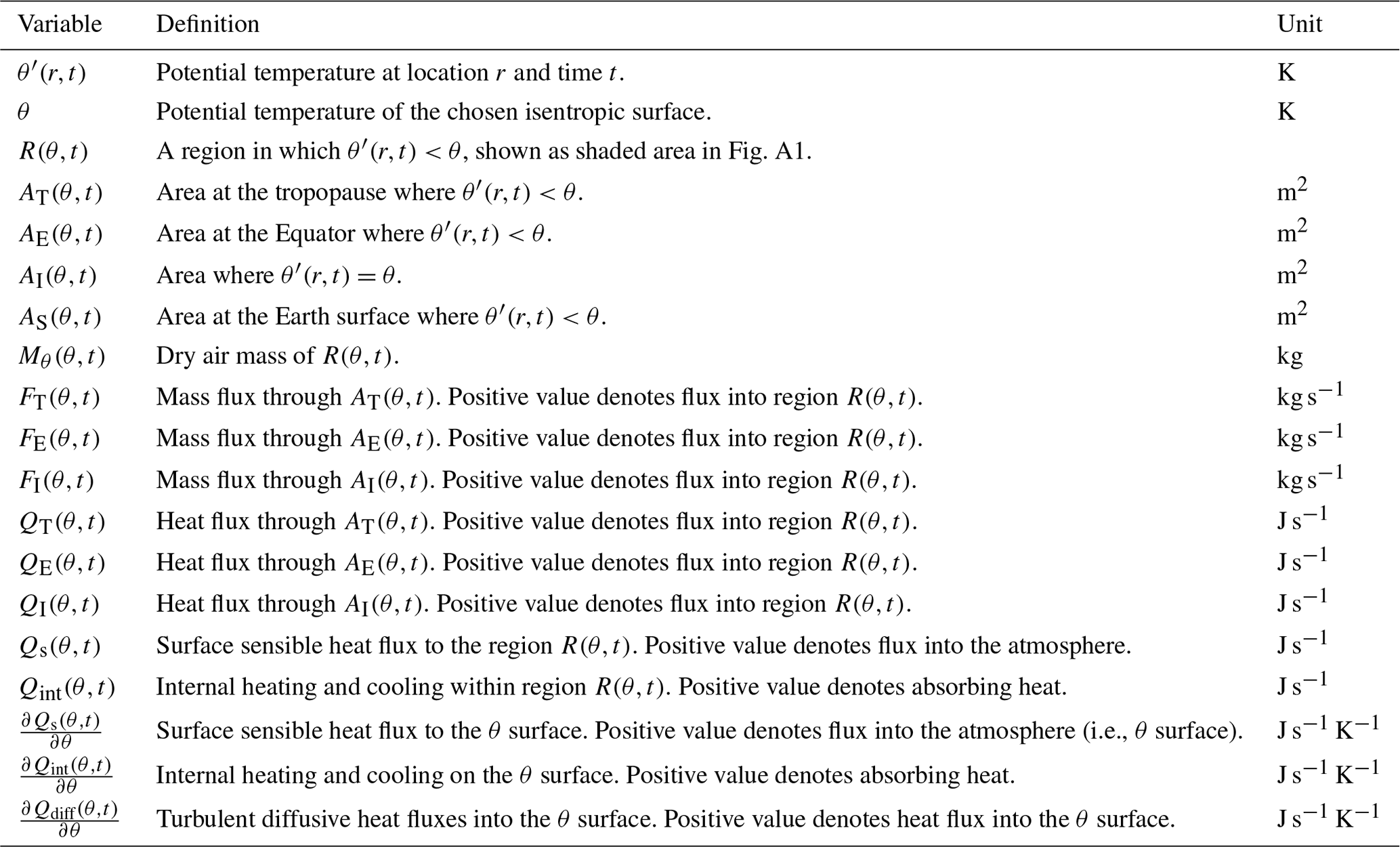
All definitions are summarized in Table A1, and Fig. A1 is the schematic diagram of mass and energy flux.
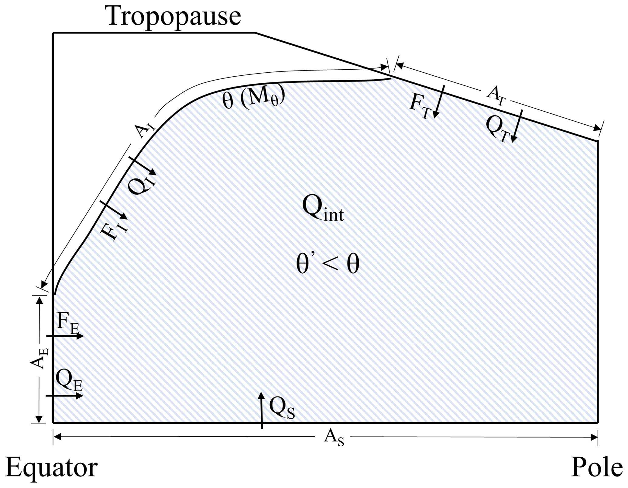
Figure A1Illustration of terms defined in Table A1. Shaded area denotes the region R(θ,t) with θ′ lower than θ, which is the area of mass integration to yield Mθ. The curve denotes a given θ or Mθ surface.
All mass and heat fluxes into region R(θ,t) are counted as positive. The heat fluxes through the tropopause, Equator, and surface of region R(θ,t) can be divided into an advective (F(θ,t)) and a turbulent (D(θ,t)) component. Integrating over the tropopause and equatorial boundary, we have
where Cpd is the heat capacity of dry air in units of J kg−1 K−1.
Based on the continuity of mass and energy for region R(θ,t), we obtain
Substituting Eqs. (A1) to (A3) into Eq. (A5) and differentiating with respect to θ yields
where
Differentiating Eq. (A4) with respect to θ and multiplying Cpd⋅θ yields
Subtracting Eq. (A8) from Eq. (A6), we obtain
Equation (A9) divided by Cpd plus Eq. (A4) yields
Equation (A10) illustrates the temporal variation in Mθ, where Qint includes radiative heating (i.e., sum of shortwave and longwave heating), dissipation of the kinetic energy of turbulence, and latent heat release due to evaporation and condensation.
To modify Eq. (A10) to apply to rather than to Mθ, it is necessary to replace all θ with θe and additionally account for the following:
-
Condensation and evaporation is conserved on the θe surfaces, but the gaining and losing of water vapor through surface evaporation and water vapor transport contributes to θe. This contribution can be computed as the product of latent heat of evaporation and the extra water vapor content. Thus, the surface contribution (QS) needs to include both sensible heating of the atmosphere (Qsen) and the water vapor flux from the surface into the atmosphere (Qevap). Similarly, the diffusion term within the atmosphere (Qdiff) needs to include both heat and water vapor ().
-
Internal heating (Qint) needs to exclude latent heat releasing due to evaporation and condensation of liquid water, which cancel in θe, but it still needs to include heating from ice formation, which does not cancel in θe. We subtract this ice component from the rest of the internal heating, yielding two terms and Qice, with .
Therefore, we can write the temporal variation in as
We provide R code to generate θe– look-up tables from ERA-Interim meteorological fields at https://doi.org/10.5281/zenodo.4420417 (Jin, 2021a).
All HIPPO 10 s merge data are available from https://doi.org/10.3334/CDIAC/HIPPO_010 (Wofsy et al., 2017b). Besides, all HIPPO Medusa merge data are available from https://doi.org/10.3334/CDIAC/HIPPO_014 (Wofsy et al., 2017a). All ATom 10 s and Medusa merge data are available from https://doi.org/10.3334/ORNLDAAC/1581 (Wofsy et al., 2018).
CO2 data from Mauna Loa Observatory are available from the Scripps CO2 Program at https://scrippsco2.ucsd.edu/assets/data/atmospheric/stations/in_situ_co2/monthly/monthly_in_situ_co2_mlo.csv (last access: 10 July 2020; Keeling et al., 2001.). Other surface station CO2 data, including Trinidad Head, Cold Bay, Barrow, Cape Kumukahi, and Sand Island, are provided by the NOAA ESRL GMD flask sampling network (http://www.cmdl.noaa.gov/ccgg/trends, last access: 9 July 2020) and downloaded from Observation Package (ObsPack) at https://doi.org/10.25925/20190812 (Cooperative Global Atmospheric Data Integration Project, 2019).
The Jena CO2 inversion data are available at the project website: https://doi.org/10.17871/CarboScope-s04oc_v4.3 (Rödenbeck, 2005). Run ID s04oc v4.3 was used in this study.
θe– look-up tables with daily resolution and 1 K intervals in θe from 1980 to 2018 computed from ERA-Interim are available at https://doi.org/10.5281/zenodo.4420398 (Jin, 2021b).
The supplement related to this article is available online at: https://doi.org/10.5194/acp-21-217-2021-supplement.
YJ carried out the data analysis and derivations. All sections in the initial draft were prepared by YJ and RFK, with critical revisions from all co-authors. BBS made important contributions to the improvement of the application part. EJM and NCP raised useful suggestions regarding the definition of . ER provided valuable suggestions for analyzing the relationship between diabatic heating and mass fluxes.
The authors declare that they have no conflict of interest.
Any opinions, findings, and conclusions or recommendations expressed in this material are those of the authors and do not necessarily reflect the views of the National Science Foundation.
The original concept arose out of discussions during the ORCAS field campaign that included Ralph F. Keeling, Colm Sweeney, Eric Kort, Matthew Long, and Martin Hoecker-Martinez. We would like to acknowledge the efforts of the full HIPPO and ATom science teams and the pilots and crew of the NSF/NCAR GV and NASA DC-8 as well as the NCAR and NASA project managers, field support staff, and logistics experts. In this work, we have used the HIPPO and ATom 10 s merge files, supported by the National Center for Atmospheric Research (NCAR). NCAR is sponsored by the National Science Foundation under Cooperative Agreement No. 1852977. We thank the Harvard QCLS, Harvard OMS, NOAA UCATS, and NOAA Picarro teams for sharing measurements. We thank NOAA ESRL GML for providing surface station CO2 data measured at Trinidad Head, Cold Bay, Barrow, Cape Kumukahi, and Sand Island. We thank Christian Rödenbeck for sharing the Jena CO2 inversion run. We thank the two anonymous reviewers for their valuable comments and efforts.
This research has been supported by the National Science Foundation (grant nos. ATM-0628575, ATM-0628519, ATM-0628388, AGS-1547797, and AGS-1623748) and the NASA (grant no. NNX15AJ23G).
This paper was edited by Andreas Engel and reviewed by two anonymous referees.
Arora, K., Cazenave, A., Engdahl, E. R., Kind, R., Manglik, A., Roy, S., Sain, K., and Uyeda, S.: Encyclopedia of solid earth geophysics, Springer, Dordrecht, the Netherlands, 2011.
Bailey, A., Singh, H. K. A., and Nusbaumer, J.: Evaluating a Moist Isentropic Framework for Poleward Moisture Transport: Implications for Water Isotopes Over Antarctica, Geophys. Res. Lett., 46, 7819–7827, https://doi.org/10.1029/2019GL082965, 2019.
Barnes, E. A., Parazoo, N., Orbe, C., and Denning, A. S.: Isentropic transport and the seasonal cycle amplitude of CO2, J. Geophys. Res.-Atmos., 121, 8106–8124, https://doi.org/10.1002/2016JD025109, 2016.
Bent, J. D.: Airborne oxygen measurements over the Southern Ocean as an integrated constraint of seasonal biogeochemical processes, University of California, San Diego, USA, 2014.
Birner, T., Do, A., and Schumann, U.: How sharp is the tropopause at midlatitudes?, Geophys. Res. Lett., 29, 1–4, https://doi.org/10.1029/2002GL015142, 2002.
Bolton, D.: The computation of equivalent potential temperature, Mon. Weather Rev., 108, 1046–1053, https://doi.org/10.1175/1520-0493(1980)108<1046:TCOEPT>2.0.CO;2, 1980.
Bozem, H., Hoor, P., Kunkel, D., Köllner, F., Schneider, J., Herber, A., Schulz, H., Leaitch, W. R., Aliabadi, A. A., Willis, M. D., Burkart, J., and Abbatt, J. P. D.: Characterization of transport regimes and the polar dome during Arctic spring and summer using in situ aircraft measurements, Atmos. Chem. Phys., 19, 15049–15071, https://doi.org/10.5194/acp-19-15049-2019, 2019.
Butchart, N. and Remsberg, E. E.: The area of the stratospheric polar vortex as a diagnostic for tracer transport on an isentropic surface, J. Atmos. Sci., 43, 1319–1339, https://doi.org/10.1175/1520-0469(1986)043<1319:TAOTSP>2.0.CO;2, 1986.
Conway, T. J. and Tans, P. P.: Development of the CO2 latitude gradient in recent decades, Global Biogeochem. Cy., 13, 821–826, https://doi.org/10.1029/1999GB900045, 1999.
Cooperative Global Atmospheric Data Integration Project: Multi-laboratory compilation of atmospheric carbon dioxide data for the period 1957–2018; obspack_co2_1_GLOBALVIEWplus_v5.0_2019_08_12, NOAA Earth System Research Laboratory, Global Monitoring Division, https://doi.org/10.25925/20190812, 2019.
Dee, D. P., Uppala, S. M., Simmons, A. J., Berrisford, P., Poli, P., Kobayashi, S., Andrae, U., Balmaseda, M. A., Balsamo, G., Bauer, P., Bechtold, P., Beljaars, A. C. M., van de Berg, L., Bidlot, J., Bormann, N., Delsol, C., Dragani, R., Fuentes, M., Geer, A. J., Haimberger, L., Healy, S. B., Hersbach, H., Hólm, E. V., Isaksen, L., Kållberg, P., Köhler, M., Matricardi, M., Mcnally, A. P., Monge-Sanz, B. M., Morcrette, J. J., Park, B. K., Peubey, C., de Rosnay, P., Tavolato, C., Thépaut, J. N., and Vitart, F.: The ERA-Interim reanalysis: Configuration and performance of the data assimilation system, Q. J. Roy. Meteor. Soc., 137, 553–597, https://doi.org/10.1002/qj.828, 2011.
Dima, I. M. and Wallace, J. M.: On the Seasonality of the Hadley Cell, J. Atmos. Sci., 60, 1522–1527, https://doi.org/10.1175/1520-0469(2003)060<1522:OTSOTH>2.0.CO;2, 2003.
Ehhalt, D. H.: The CH4 concentration over the ocean and its possible variation with latitude, Tellus, 30, 169–176, https://doi.org/10.3402/tellusa.v30i2.10329, 1978.
Fasullo, J. T. and Trenberth, K. E.: The annual cycle of the energy budget. Part I: Global mean and land-ocean exchanges, J. Climate, 21, 2297–2312, https://doi.org/10.1175/2007JCLI1935.1, 2008.
Foltz, G. R. and McPhaden, M. J.: The role of oceanic heat advection in the evolution of tropical North and South Atlantic SST anomalies, J. Climate, 19, 6122–6138, https://doi.org/10.1175/JCLI3961.1, 2006.
Gelaro, R., McCarty, W., Suárez, M. J., Todling, R., Molod, A., Takacs, L., Randles, C. A., Darmenov, A., Bosilovich, M. G., Reichle, R., Wargan, K., Coy, L., Cullather, R., Draper, C., Akella, S., Buchard, V., Conaty, A., da Silva, A. M., Gu, W., Kim, G. K., Koster, R., Lucchesi, R., Merkova, D., Nielsen, J. E., Partyka, G., Pawson, S., Putman, W., Rienecker, M., Schubert, S. D., Sienkiewicz, M., and Zhao, B.: The Modern-Era Retrospective Analysis for Research and Applications, Version 2 (MERRA-2), J. Climate, 30, 5419–5454, https://doi.org/10.1175/JCLI-D-16-0758.1, 2017.
Graven, H. D., Keeling, R. F., Piper, S. C., Patra, P. K., Stephens, B. B., Wofsy, S. C., Welp, L. R., Sweeney, C., Tans., P. P., Kelley, J. J., Daube, B. C., Kort, E. A., Santoni, G. W., and Bent, J. D.: Enhanced seasonal exchange of CO2 by northern ecosystems since 1960, Science, 341, 1085–1089, https://doi.org/10.1126/science.1239207, 2013.
Harris, J. M. and Kahl, J. D.: A descriptive atmospheric transport climatology for the Mauna Loa Observatory, using clustered trajectories, J. Geophys. Res.-Atmos., 95, 13651–13667, https://doi.org/10.1029/jd095id09p13651, 1990.
Harris, J. M., Tans, P. P., Dlugokencky, E. J., Masarie, K. A., Lang, P. M., Whittlestone, S., and Steele, L. P.: Variations in atmospheric methane at Mauna Loa Observatory related to long-range transport, J. Geophys. Res.-Atmos., 97, 6003–6010, https://doi.org/10.1029/92JD00158, 1992.
Hoskins, B. J. and Karoly, D. J.: The Steady Linear Response of a Spherical Atmosphere to Thermal and Orographic Forcing, J. Atmos. Sci., 38, 1179–1196, https://doi.org/10.1175/1520-0469(1981)038<1179:TSLROA>2.0.CO;2, 1981.
Hurst, D.: UCATS 2-Channel Gas Chromatograph (GC), Version 1.0, UCAR/NCAR Earth Observing Laboratory, Global Monitoring Division (GMD), Earth System Research Laboratory, NOAA, available at: https://data.eol.ucar.edu/dataset/112.021 (last access: 10 May 2020), 2011.
Jacob, D. J.: Introduction to atmospheric chemistry, Princeton University Press, New Jersey, USA, 1999.
Jin, Y.: yumingjin0521/Mthetae: θ-Mθe Lookup Table Computation Method (Version v1.0.0), Zenodo, https://doi.org/10.5281/zenodo.4420417, 2021a.
Jin, Y.: θ-Mθe Lookup Table (ERA-Interim) (Version v1.0.0) [Data set], Zenodo, https://doi.org/10.5281/zenodo.4420398, 2021b.
Kanamitsu, M., Ebisuzaki, W., Woollen, J., Yang, S.-K., Hnilo, J. J., Fiorino, M., and Potter, G. L.: NCEP-DOE AMIP-II Renalalysys (R-2), B. Am. Meteorol. Soc., 83, 1631–1643, https://doi.org/10.1175/BAMS-83-11-1631, 2002.
Keeling, C. D., Piper, S. C., Bacastow, R. B., Wahlen, M., Whorf, T. P., Heimann, M., and Meijer, H. A.: Exchanges of atmospheric CO2 and 13CO2 with the terrestrial biosphere and oceans from 1978 to 2000. I. Global aspects, SIO Reference Series, No. 01-06, Scripps Institution of Oceanography, San Diego, USA, 88 pp., 2001.
Keppel-Aleks, G., Wennberg, P. O., and Schneider, T.: Sources of variations in total column carbon dioxide, Atmos. Chem. Phys., 11, 3581–3593, https://doi.org/10.5194/acp-11-3581-2011, 2011.
Li, Z. and Leighton, H. G.: Global climatologies of solar radiation budgets at the surface and in the atmosphere from 5 years of ERBE data, J. Geophys. Res.-Atmos., 98, 4919–4930, https://doi.org/10.1029/93jd00003, 1993.
Linz, M., Plumb, R. A., GerBer, E. P., and Sheshadri, A.: The Relationship between Age of Air and the Diabatic Circulation of the Stratosphere, J. Atmos. Sci., 73, 4507–4518, https://doi.org/10.1175/JAS-D-16-0125.1, 2016.
Miyazaki, K. and Iwasaki, T.: Diagnosis of Meridional Ozone Transport Based on Mass-Weighted Isentropic Zonal Means, J. Atmos. Sci., 62, 1192–1208, https://doi.org/10.1175/JAS3394.1, 2005.
Miyazaki, K., Patra, P. K., Takigawa, M., Iwasaki, T., and Nakazawa, T.: Global-scale transport of carbon dioxide in the troposphere, J. Geophys. Res.-Atmos., 113, D15301, https://doi.org/10.1029/2007JD009557, 2008.
Mooney, P. A., Mulligan, F. J., and Fealy, R.: Comparison of ERA-40, ERA-Interim and NCEP/NCAR reanalysis data with observed surface air temperatures over Ireland, Int. J. Climatol., 31, 545–557, https://doi.org/10.1002/joc.2098, 2011.
Parazoo, N. C., Denning, A. S., Kawa, S. R., Corbin, K. D., Lokupitiya, R. S., and Baker, I. T.: Mechanisms for synoptic variations of atmospheric CO2 in North America, South America and Europe, Atmos. Chem. Phys., 8, 7239–7254, https://doi.org/10.5194/acp-8-7239-2008, 2008.
Parazoo, N. C., Denning, A. S., Berry, J. A., Wolf, A., Randall, D. A., Kawa, S. R., Pauluis, O., and Doney, S. C.: Moist synoptic transport of CO2 along the mid-latitude storm track, Geophys. Res. Lett., 38, L09804, https://doi.org/10.1029/2011GL047238, 2011.
Parazoo, N. C., Denning, A. S., Kawa, S. R., Pawson, S., and Lokupitiya, R.: CO2 flux estimation errors associated with moist atmospheric processes, Atmos. Chem. Phys., 12, 6405–6416, https://doi.org/10.5194/acp-12-6405-2012, 2012.
Pauluis, O., Czaja, A., and Korty, R.: The global atmospheric circulation on moist isentropes, Science, 321, 1075–1078, https://doi.org/10.1126/science.1159649, 2008.
Pauluis, O., Czaja, A., and Korty, R.: The global atmospheric circulation in moist isentropic coordinates, J. Climate, 23, 3077–3093, https://doi.org/10.1175/2009JCLI2789.1, 2010.
Petropavlovskikh, I., Hoor, P., Millán, L., Jordan, A., Kunkel, D., Leblanc, T., Manney, G., and Damadeo, R.: An Overview of OCTAV-UTLS (Observed Composition Trends and Variability in the UTLS), a SPARC Activity, EGU General Assembly 2019, 7–12 April 2019, Vienna, Austria, EGU2019-12206-2, 2019.
Prather, M. J., Flynn, C. M., Fiore, A., Correa, G., Strode, S. A., Steenrod, S. D., Murray, L. T., and Lamarque, J. F.: ATom: Simulated Data Stream for Modeling ATom-like Measurements, ORNL DAAC, Oak Ridge, Tennessee, USA, https://doi.org/10.3334/ORNLDAAC/1597, 2018.
Randerson, T., Thompson, V., Conway, J., Fung, I. Y., and Field, B.: The contribution of terrestrial sources and sinks to trends in the seasonal cycle of atmospheric carbon dioxide, Global Biogeochem. Cy., 11, 535–560, https://doi.org/10.1029/97GB02268, 1997.
Rasmussen, R. A. and Khalil, R. A. K.: Atmospheric Methane (CH4): Trends and Seasonal Cycles, J. Geophys. Res., 86, 9826–9832, https://doi.org/10.1029/JC086iC10p09826, 1981.
Rödenbeck, C.: Estimating CO2 sources and sinks from atmospheric mixing ratio measurements using a global inversion of atmospheric transport, Technical Report 6, Max Planck Institute for Biogeochemistry, Jena, Germany, https://doi.org/10.17871/CarboScope-s04oc_v4.3, 2005.
Rödenbeck, C., Houweling, S., Gloor, M., and Heimann, M.: CO2 flux history 1982–2001 inferred from atmospheric data using a global inversion of atmospheric transport, Atmos. Chem. Phys., 3, 1919–1964, https://doi.org/10.5194/acp-3-1919-2003, 2003.
Santoni, G. W., Daube, B. C., Kort, E. A., Jiménez, R., Park, S., Pittman, J. V., Gottlieb, E., Xiang, B., Zahniser, M. S., Nelson, D. D., McManus, J. B., Peischl, J., Ryerson, T. B., Holloway, J. S., Andrews, A. E., Sweeney, C., Hall, B., Hintsa, E. J., Moore, F. L., Elkins, J. W., Hurst, D. F., Stephens, B. B., Bent, J., and Wofsy, S. C.: Evaluation of the airborne quantum cascade laser spectrometer (QCLS) measurements of the carbon and greenhouse gas suite – CO2, CH4, N2O, and CO – during the CalNex and HIPPO campaigns, Atmos. Meas. Tech., 7, 1509–1526, https://doi.org/10.5194/amt-7-1509-2014, 2014.
Stephens, B. B., Morgan, E. J., Bent, J. D., Keeling, R. F., Watt, A. S., Shertz, S. R., and Daube, B. C.: Airborne measurements of oxygen concentration from the surface to the lower stratosphere and pole to pole, Atmos. Meas. Tech. Discuss., https://doi.org/10.5194/amt-2020-294, in review, 2020.
Stull, R. B.: An introduction to boundary layer meteorology, Springer, Dordrecht, the Netherlands, 2012.
Sweeney, C., Karion, A., Wolter, S., Newberger, T., Guenther, D., Higgs, J. A., Andrews, A. E., Lang, P. M., Neff, D., Dlugokencky, E., Miller, J. B., Montzka, S. A., Miller, B. R., Masarie, K. A., Biraud, S. C., Novelli, P. C., Crotwell, M., Crotwell, A. M., Thoning, K., and Tans, P. P.: Seasonal climatology of CO2 across North America from aircraft measurements in the NOAA/ESRL Global Greenhouse Gas Reference Network, J. Geophys. Res.-Atmos., 120, 5155–5190, https://doi.org/10.1002/2014JD022591, 2015.
Tohjima, Y., Minejima, C., Mukai, H., MacHida, T., Yamagishi, H., and Nojiri, Y.: Analysis of seasonality and annual mean distribution of atmospheric potential oxygen (APO) in the Pacific region, Global Biogeochem. Cy., 26, 1–15, https://doi.org/10.1029/2011GB004110, 2012.
Tung, K. K.: On the Two-Dimensional Transport of Stratospheric Tracer Gases in Isentropic Coordinates, J. Atmos. Sci., 39, 2330–2355, https://doi.org/10.1175/1520-0469(1982)039<2330:OTTDTO>2.0.CO;2, 1982.
Walin, G.: On the relation between sea-surface heat flow and thermal circulation in the ocean, Tellus, 34, 187–195, https://doi.org/10.3402/tellusa.v34i2.10801, 1982.
Wang, J. W., Denning, A. S., Lu, L., Baker, I. T., Corbin, K. D., and Davis, K. J.: Observations and simulations of synoptic, regional, and local variations in atmospheric CO2, J. Geophys. Res.-Atmos., 112, D04108, https://doi.org/10.1029/2006JD007410, 2007.
Wexler, A.: Vapor pressure equation for water in the range 0 to 100∘ C, J. Res. Natl. Bur. Stand. Sect. A Phys. Chem., 80A, 775–785, https://doi.org/10.6028/jres.075a.022, 1976.
Wills, R. C. J. and Schneider, T.: Mechanisms setting the strength of orographic Rossby waves across a wide range of climates in a moist idealized GCM, J. Climate, 31, 7679–7700, https://doi.org/10.1175/JCLI-D-17-0700.1, 2018.
Wofsy, S. C.: HIAPER Pole-to-Pole Observations (HIPPO): fine-grained, global-scale measurements of climatically important atmospheric gases and aerosols, Philos. T. Roy. Soc. A Math. Phys. Eng. Sci., 369, 2073–2086, https://doi.org/10.1098/rsta.2010.0313, 2011.
Wofsy, S., Daube, B., Jimenez, R., Kort, E., Pittman, J., Park, S., Commane, R., Xiang, B., Santoni, G., Jacob, D., Fisher, J., Pickett-Heaps, C., Wang, H., Wecht, K., Wang, Q., Stephens, B., Shertz, S., Watt, A., Romashkin, P., Campos, T., Haggerty, J., Cooper, W., Rogers, D., Beaton, S., Hendershot, R., Elkins, J., Fahey, D., Gao, R., Moore, F., Montzka, S., Schwarz, J., Perring, A., Hurst, D., Miller, B., Sweeney, C., Oltmans, S., Nance, D., Hintsa, E., Dutton, G., Watts, L., Spackman, J., Rosenlof, K., Ray, E., Hall, B., Zondlo, M., Diao, M., Keeling, R., Bent, J., Atlas, E., Lueb, R., and Mahoney, M. J.: HIPPO MEDUSA Flask Sample Trace Gas And Isotope Data, Version 1.0, UCAR/NCAR – Earth Observing Laboratory. https://doi.org/10.3334/CDIAC/HIPPO_014, 2017a.
Wofsy, S., Daube, B., Jimenez, R., Kort, E., Pittman, J., Park, S., Commane, R., Xiang, B., Santoni, G., Jacob, D., Fisher, J., Pickett-Heaps, C., Wang, H., Wecht, K., Wang, Q., Stephens, B., Shertz, S., Watt, A., Romashkin, P., Campos, T., Haggerty, J., Cooper, W., Rogers, D., Beaton, S., Hendershot, R., Elkins, J., Fahey, D., Gao, R., Moore, F., Montzka, S., Schwarz, J., Perring, A., Hurst, D., Miller, B., Sweeney, C., Oltmans, S., Nance, D., Hintsa, E., Dutton, G., Watts, L., Spackman, J., Rosenlof, K., Ray, E., Hall, B., Zondlo, M., Diao, M., Keeling, R., Bent, J., Atlas, E., Lueb, R., and Mahoney, M. J.: HIPPO Merged 10-Second Meteorology, Atmospheric Chemistry, and Aerosol Data, Version 1.0, UCAR/NCAR – Earth Observing Laboratory. https://doi.org/10.3334/CDIAC/HIPPO_010, 2017b.
Wofsy, S. C., Afshar, S., Allen, H. M., Apel, E., Asher, E. C., Barletta, B., Bent, J., Bian, H., Biggs, B. C., Blake, D. R., Blake, N., Bourgeois, I., Brock, C. A., Brune, W. H., Budney, J. W., Bui, T. P., Butler, A., Campuzano-Jost, P., Chang, C. S., Chin, M., Commane, R., Correa, G., Crounse, J. D., Cullis, P. D., Daube, B. C., Day, D. A., Dean-Day, J. M., Dibb, J. E., Digangi, J. P., Diskin, G. S., Dollner, M., Elkins, J. W., Erdesz, F., Fiore, A. M., Flynn, C. M., Froyd, K., Gesler, D. W., Hall, S. R., Hanisco, T. F., Hannun, R. A., Hills, A. J., Hintsa, E. J., Hoffman, A., Hornbrook, R. S., Huey, L. G., Hughes, S., Jimenez, J. L., Johnson, B. J., Katich, J. M., Keeling, R., Kim, M. J., Kupc, A., Lait, L. R., Lamarque, J. F., Liu, J., McKain, K., McLaughlin, R. J., Meinardi, S., Miller, D. O., Montzka, S. A., Moore, F. L., Morgan, E. J., Murphy, D. M., Murray, L. T., Nault, B. A., Neuman, J. A., Newman, P. A., Nicely, J. M., Pan, X., Paplawsky, W., Peischl, J., Prather, M. J., Price, D. J., Ray, E., Reeves, J. M., Richardson, M., Rollins, A. W., Rosenlof, K. H., Ryerson, T. B., Scheuer, E., Schill, G. P., Schroder, J. C., Schwarz, J. P., St. Clair, J. M., Steenrod, S. D., Stephens, B. B., Strode, S. A., Sweeney, C., Tanner, D., Teng, A. P., Thames, A. B., Thompson, C. R., Ullmann, K., Veres, P. R., Vizenor, N., Wagner, N. L., Watt, A., Weber, R., Weinzierl, B., Wennberg, P. O., Williamson, C. J., Wilson, J. C., Wolfe, G. M., Woods, C. T., and Zeng, L. H.: ATom: Merged Atmospheric Chemistry, Trace Gases, and Aerosols, ORNL DAAC, https://doi.org/10.3334/ORNLDAAC/1581, 2018.
Yang, H., Chen, G., Tang, Q., and Hess, P.: Quantifying isentropic stratosphere-troposphere exchange of ozone, J. Geophys. Res.-Atmos., 121, 3372–3387, https://doi.org/10.1002/2015JD024180, 2016.
- Abstract
- Introduction
- Methods
- Characteristics of
- Applications of as an atmospheric coordinate
- Discussion and summary
- Appendix A: Temporal variation in
- Code availability
- Data availability
- Author contributions
- Competing interests
- Disclaimer
- Acknowledgements
- Financial support
- Review statement
- References
- Supplement