the Creative Commons Attribution 4.0 License.
the Creative Commons Attribution 4.0 License.
 | 01 Dec 2021
Quantification of CH4 coal mining emissions in Upper Silesia by passive airborne remote sensing observations with the Methane Airborne MAPper (MAMAP) instrument during the CO2 and Methane (CoMet) campaign
Sven Krautwurst
Konstantin Gerilowski
Jakob Borchardt
Norman Wildmann
Michał Gałkowski
Justyna Swolkień
Julia Marshall
Alina Fiehn
Anke Roiger
Thomas Ruhtz
Christoph Gerbig
Jaroslaw Necki
John P. Burrows
Andreas Fix
Heinrich Bovensmann
Methane (CH4) is the second most important anthropogenic greenhouse gas, whose atmospheric concentration is modulated by human-induced activities, and it has a larger global warming potential than carbon dioxide (CO2). Because of its short atmospheric lifetime relative to that of CO2, the reduction of the atmospheric abundance of CH4 is an attractive target for short-term climate mitigation strategies. However, reducing the atmospheric CH4 concentration requires a reduction of its emissions and, therefore, knowledge of its sources.
For this reason, the CO2 and Methane (CoMet) campaign in May and June 2018 assessed emissions of one of the largest CH4 emission hot spots in Europe, the Upper Silesian Coal Basin (USCB) in southern Poland, using top-down approaches and inventory data. In this study, we will focus on CH4 column anomalies retrieved from spectral radiance observations, which were acquired by the 1D nadir-looking passive remote sensing Methane Airborne MAPper (MAMAP) instrument, using the weighting-function-modified differential optical absorption spectroscopy (WFM-DOAS) method. The column anomalies, combined with wind lidar measurements, are inverted to cross-sectional fluxes using a mass balance approach. With the help of these fluxes, reported emissions of small clusters of coal mine ventilation shafts are then assessed.
The MAMAP CH4 column observations enable an accurate assignment of observed fluxes to small clusters of ventilation shafts. CH4 fluxes are estimated for four clusters with a total of 23 ventilation shafts, which are responsible for about 40 % of the total CH4 mining emissions in the target area. The observations were made during several overflights on different days. The final average CH4 fluxes for the single clusters (or sub-clusters) range from about 1 to 9 t CH4 h−1 at the time of the campaign. The fluxes observed at one cluster during different overflights vary by as much as 50 % of the average value. Associated errors (1σ) are usually between 15 % and 59 % of the average flux, depending mainly on the prevailing wind conditions, the number of flight tracks, and the magnitude of the flux itself. Comparison to known hourly emissions, where available, shows good agreement within the uncertainties. If only emissions reported annually are available for comparison with the observations, caution is advised due to possible fluctuations in emissions during a year or even within hours. To measure emissions even more precisely and to break them down further for allocation to individual shafts in a complex source region such as the USCB, imaging remote sensing instruments are recommended.
- Article
(7223 KB) - Full-text XML
- BibTeX
- EndNote


The release of greenhouse gases from anthropogenic activity significantly influences the atmospheric surface temperature (Stocker et al., 2013). Consequently, the need to reduce these emissions is well-recognized (Fesenfeld et al., 2018; UNFCCC, 2015, 1998). The increase in carbon dioxide (CO2) induces the largest impact on the surface temperature with a radiative forcing (RF) of ∼1.8 W m−2 (Etminan et al., 2016). The second largest increase in anthropogenic radiative forcing results from the increase in methane (CH4) with ∼0.6 W m−2 (Etminan et al., 2016). However, on a per mass basis, CH4 is 34 times more efficient in trapping heat in the Earth's atmosphere over 100 years than CO2 (Myhre et al., 2013, including climate–carbon feedbacks). Moving to shorter timescales (e.g. 20 years), the effectiveness (or the global warming potential, GWP) of CH4 rises to 86 times that of CO2 (Myhre et al., 2013, including climate–carbon feedbacks). The high GWP of CH4 in combination with a short atmospheric lifetime of around 9 years (Prather et al., 2012) makes CH4 an attractive target for short-term emission reduction and, thus, climate mitigation strategies (Saunois et al., 2016; Shindell et al., 2012).
To reduce methane emissions, their emission strengths and also locations need to be known. However, current knowledge is inadequate as evidenced by the discussion about the origin of increasing atmospheric CH4 concentrations observed since 2007 (Dlugokencky et al., 2011). Depending on the applied methodology (e.g. measuring ethane-to-methane ratio or isotopic analysis), authors either conclude that CH4 emissions from fossil fuels (Franco et al., 2016; Hausmann et al., 2016; Helmig et al., 2016; Turner et al., 2016) or from wetlands and agriculture (Nisbet et al., 2016; Schaefer et al., 2016; Schwietzke et al., 2016) have increased or that the increase in atmospheric CH4 is even related to a decline in atmospheric OH, which removes the CH4 (Rigby et al., 2017; Turner et al., 2017). Interestingly, even though Schwietzke et al. (2016) concluded that the increase is mostly related to wetlands and agriculture, they further stated that global emissions from the fossil fuel industry could be ∼40 % higher than previously expected by Saunois et al. (2016). A study by Petrenko et al. (2017) supports this hypothesis and finds indications that even this revised number might be too low by at least 25 %. A recent study from Jackson et al. (2020) also concluded that the global increase in atmospheric CH4 has been mostly driven by anthropogenic emissions, and natural CH4 emissions remained almost unaltered between the period 2000–2006 and 2017. However, not only on a global scale but also on smaller scales is our knowledge and characterization of fossil fuel CH4 emissions inadequate (e.g. Buchwitz et al., 2017; Maasakkers et al., 2016; Alexe et al., 2015; Turner et al., 2015).
A large source of anthropogenically emitted CH4 originates from coal mining. It globally accounts for around one-tenth of the anthropogenic CH4 emissions of about 350 Mt CH4 yr−1 (Saunois et al., 2016, 2020). China, the largest emitter of CH4 from coal mining, is responsible for ∼50 % of the global total (EPA, 2012). The share of the European Union is around 4 %, with the largest contribution originating from Poland. This country is also home to the largest contemporary hard coal mining area in Europe, located in the Upper Silesian Coal Basin (USCB), occupying around 7400 km2 (Gzyl et al., 2017) in total and extending into the Czech Republic (compare Fig. 1, area in Poland is around 5400 km2).
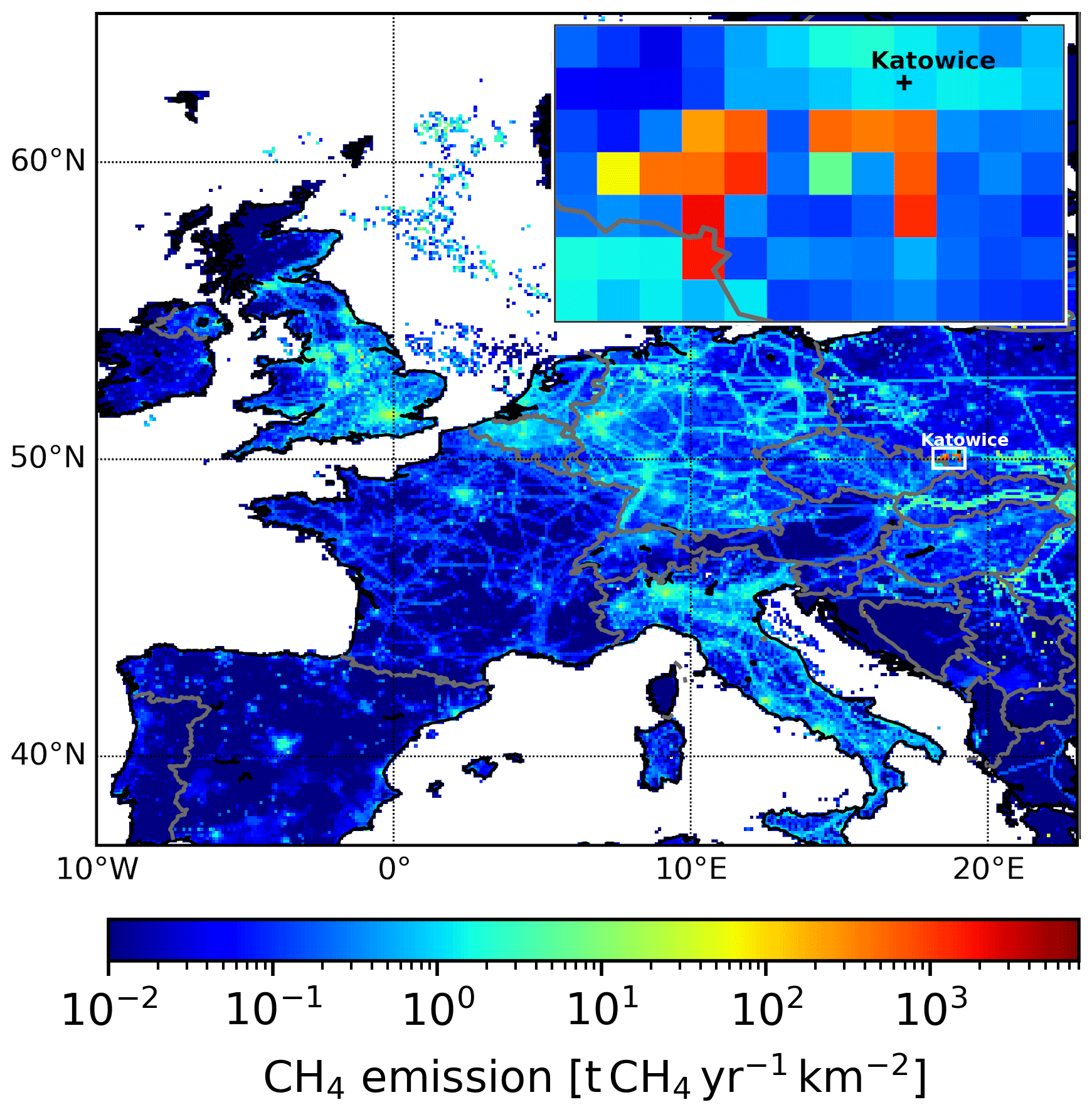
Figure 1European CH4 emissions from fossil fuels in 2016. The Upper Silesian Coal Basin (USCB) is located around 50∘ N, 19∘ E and framed by the white rectangle. A magnification is shown in the inset. Emission map is based on data from Scarpelli et al. (2020).
According to the latest bottom-up inventories (i.e. emissions calculated from emission factors and activity data), the EDGAR v4.3.21 inventory for 2012 (Janssens-Maenhout et al., 2019) and v5.02 for 2015 (Crippa et al., 2020), and an inventory specially designed for fossil fuel emissions from Scarpelli et al. (2020) for 2016, annual fossil fuel CH4 emissions range from about 550 to 820 kt CH4 yr−1 (or 63 to 94 t CH4 h−1) in that region. The largest contribution is attributed to coal mining activities, depending on the inventory between 87 % (Crippa et al., 2020) and 99 % (Scarpelli et al., 2020). The geological structure of the deposit located in the USCB region favours gas migration. The methane content in the USCB deposits is highly diversified and increases with depth. It changes even throughout the coal mine. In the USCB mining areas, it can change between 4 to even above 16 m3 t−1 daf (dry ash free). The potential to generate methane from 1 t of extracted coal is described as a specific methane emission, which for the USCB Polish coal deposits reached 14.4 m3 t−1 in 2018. The coal output was equal to 63.4 Mt yr−1 in 2018. Detailed information about variability of methane emissions and the measurement procedure will be subject of another study in the CoMet special issue (Swolkien et al., 2021).
The Carbon dioxide and Methane (CoMet) campaign was performed in May and June 2018 to investigate this European CH4 emission hot spot. One of its main goals was the estimation of CH4 emissions from coal mining by using top-down approaches and assessing the available inventory data. In this study, we investigate the emission estimates from observations made by the airborne passive remote sensing instrument MAMAP (Methane Airborne MAPper; Gerilowski et al., 2011) and wind lidar observations for different groups of ventilation shafts. This study covers spatial scales in between those of already published analyses from the campaign. Nickl et al. (2020) performed model simulations and Fiehn et al. (2020) computed fluxes from airborne in situ observations for the entire basin, whereas Luther et al. (2019) estimated emissions from individual shafts by means of mobile on-the-ground FTS (Fourier transform spectrometer) observations. Further studies including the synergistic use of instruments and models are planned as part of the special issue “CoMet: a mission to improve our understanding and to better quantify the carbon dioxide and methane cycles”.
This article is organized as follows. Section 2 introduces the methods applied. This comprises a comprehensive description of the CoMet campaign including the instrumentation (Sect. 2.1), the passive remote sensing (Sect. 2.2.1) and wind lidar (Sect. 2.2.2) observations, and the computation of cross-sectional fluxes (Sect. 2.2.3). Those fluxes are assigned to different mining clusters in Sect. 2.3, and Sect. 2.4 describes the inventory used for comparison. In Sect. 3 the results are presented, including the general wind situation on the different flight days (Sect. 3.1) and the computed fluxes for the different mining clusters (Sect. 3.2). Section 4 provides a detailed comparison and discussion on the computed fluxes and reported CH4 emissions. Finally, the results are discussed in Sect. 5, and conclusions are drawn in Sect. 6.
2.1 CoMet measurement campaign and instrumentation
The CoMet research campaign in early Summer 2018 investigated, among other things, coal mining emissions from the largest European CH4 emission hot spot, the USCB (between ∼18.3–19.2∘ E and ∼49.9–50.3∘ N) in Poland. CH4 is emitted from over 50 coal mine ventilation shafts occupying an area of around 60 km×40 km. However, common inventories (Crippa et al., 2020; Janssens-Maenhout et al., 2019; Scarpelli et al., 2020) provide CH4 emissions only at a coarse spatial resolution of (translating to km2 in the discussed area). Consequently, for optimal flight planning and also subsequent assignment of observed CH4 enhancements to specific CH4 sources, the CoMet team generated a more detailed point-source inventory. This inventory, hereafter referred to as CoMet ED (emission database) v4 (Gałkowski et al., 2021a) and described in further detail in Sect. 2.4, comprises annually reported CH4 emissions of about 530 kt CH4 yr−1 for 2018, which are assigned to 54 exactly geolocated active ventilation shafts found in the region (Fig. 2).

Figure 2Overview of the active coal mine ventilation shafts in the Upper Silesian Coal Basin (USCB, blueish triangles). Colour intensity indicates the annual CH4 emission as stated in the CoMet ED v4 inventory for the year 2018. Ventilation shafts filled with a red circle are investigated in this work and grouped in four clusters (see main text and Table 1 for details). Filled white circles give the locations of the three wind lidars deployed during the CoMet campaign (DLR85: 50.07025∘ N, 18.6298∘ E; at 250 ; DLR86: 50.3292∘ N, 19.4155∘ E; at 300 ; DLR89: 49.9326∘ N, 18.7998∘ E; at 270 ). The airport is located north of the mining region. The grey shading indicates the terrain height and the border with the Czech Republic is represented by the solid yellow line.
To investigate the CH4 emissions on different scales ranging from single shafts over smaller clusters up to the entire basin, a variety of observation platforms and instruments were deployed during the CoMet campaign. This study focuses on observations from the airborne passive remote sensing instrument MAMAP (operated by the University of Bremen; Gerilowski et al., 2011) installed aboard a Cessna aircraft operated by FUB (Freie Universität Berlin) and deployed at Katowice Airport (EPKT), Poland, at the northern edge of the mining area (see Fig. 2). The analysis and interpretation of the MAMAP data were supported by in situ concentration measurements of CH4 and CO2 by the FUB Cessna, by a Gulfstream G550 (HALO, High Altitude and Long Range Research Aircraft – operated by DLR, Deutsches Zentrum für Luft- und Raumfahrt; Fix and The CoMet Team, 2021; Gałkowski et al., 2021b), and by a second Cessna Caravan (also operated by the DLR; Fiehn et al., 2020; Kostinek et al., 2019). Additionally, wind field observations by three stationary wind lidars in that region specifically deployed for CoMet were acquired (operated by DLR; Wildmann et al., 2020). For adequate flight planning and also interpretation of the collected data sets, various model support and weather forecast systems were provided (Gałkowski et al., 2021c; Nickl et al., 2020).
The main aim of the study in hand is the estimation of the small-scale CH4 emissions from clusters of ventilation shafts by combining MAMAP observations with wind lidar data. MAMAP is a grating spectrometer, which records reflected solar radiation from the ground while flying above the planetary boundary layer (PBL) at around 3 km above ground level (a.g.l.). Spectra are recorded in the shortwave infrared (SWIR) region between 1590 and 1690 nm with a spectral resolution (full width at half maximum, FWHM) of around 0.9 nm. The ground scene size of one MAMAP pixel is around 90×100 m2 (across × along track) at a flight altitude of around ∼3 , a ground speed of ∼200 km h−1, and a total integration time of ∼1 s. Column information of CH4 is extracted using absorption spectroscopy. The retrieved CH4 column anomalies have a single-measurement precision of better than 0.4 % relative to the background column, in general. They have, for instance, been used to estimate CH4 emissions from two coal mine ventilation shafts near Ibbenbüren in Germany (Krings et al., 2013) and from landfills in Los Angeles, USA (Krautwurst et al., 2017). According to Observation System Simulation Experiments (OSSEs; for details, see, for example, Krautwurst et al., 2017, and Gerilowski et al., 2015) performed before the campaign, which considered the instrumental characteristics, the MAMAP measurement precision should be sufficient to investigate CH4 emissions in the more complex region of the USCB.
The wind information required for the flux estimates is derived from the three wind lidar systems (Leosphere WindCube 200S), which were deployed at three different locations in the USCB as shown in Fig. 2. They measure the vertically resolved wind profile at the location of the wind lidar. Data are available as 30 min averages in 50 m altitude bins. Additionally, the eddy dissipation rate is computed, from which we estimated the boundary layer height. The uncertainty of the wind speed is 0.2 m s−1 (Luther et al., 2019). Further details on the measurement principle and analysis are found in Luther et al. (2019), Stephan et al. (2018a), Stephan et al. (2018b), Smalikho and Banakh (2017), and Smalikho (2003).
MAMAP observations were acquired during six flights in the USCB between 28 May and 7 June mostly before or around noon. Usual flight duration over the mining area was 2 to 3 h each. Wind lidar observations were continuously collected throughout the entire campaign period.
2.2 Retrieval of column anomalies and inversion to emissions
2.2.1 CH4 column anomalies
During a measurement flight, the MAMAP instrument typically probes the air column below the aircraft while flying above the PBL downwind of potential emission sources. The collected spectra contain the absorption features of CH4 (and also CO2), whose strengths depend on the amount of those gases in the atmosphere. From these features, the CH4 column anomalies are retrieved using the weighting-function-modified differential optical absorption spectroscopy (WFM-DOAS) algorithm and the CH4 over CO2 proxy method, which are described in detail in Krings et al. (2011) and in Sect. A1.1.
On average, the accuracy and precision of the retrieved CH4 column anomalies are estimated to be around 0.10 % and 0.22 %, respectively, relative to the CH4 background column for this investigated data set. The single-measurement precision is directly computed from the scatter of the measured data after applying the retrieval described in Sect. A1.1 from observations which are not influenced by a CH4 plume. The accuracy considers the influence of the terrain, such as surface elevation and surface spectral reflectance, which might not be entirely accounted for during the retrieval process. A more detailed discussion of the error budget is given in Sect. A1.2.
2.2.2 Wind information
To describe the mass flow through a cross-section of column measurements, not only trace gas anomalies but also wind information is required. Ideally, the wind field is measured inside or near the emission plume simultaneously with the trace gas observations. In the current study, we have used observations from three wind lidar stations deployed in the area of interest to estimate the prevailing wind conditions inside the PBL. As an example, Fig. 3 shows the temporal evolution of the wind speed at all three stations on 7 June.
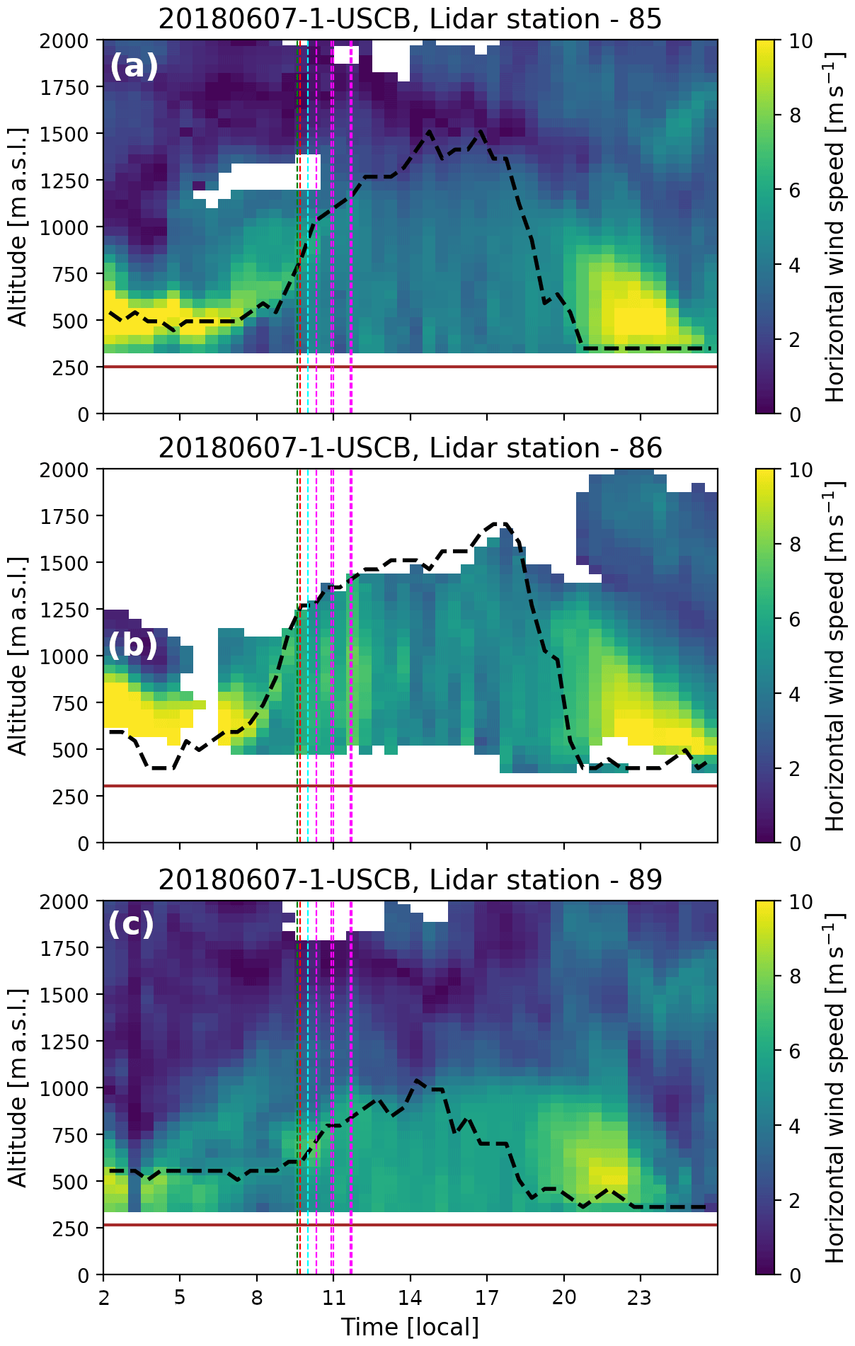
Figure 3Vertically resolved wind speed measurements on 7 June from the three lidar stations deployed in the USCB. The temporal evolution of the boundary layer height is shown by the dashed black line. Dotted vertical lines mark the time of the different MAMAP observations/overflights on that day at the four clusters (from left to right: green: cluster c, red: cluster a, cyan: cluster d, magenta: cluster b). Positions of the three lidars are marked in Fig. 2.
The wind speed and direction for each flight track are computed as (time and distance) weighted averages of all three lidar stations, only considering measurements within the PBL (Fig. 3, dashed black line). We assume that the plume is well-mixed within, and also confined by, the PBL. For each wind lidar, all wind speed and direction measurements within the PBL are averaged vertically for each time step, and then the two measurements closest in time to the overflight are averaged, weighted according to their time difference to the overflight time. Finally, the values from the three stations are averaged, weighted by their distance to the flight track. This wind speed and direction value is then used in the cross-sectional flux calculation described in the next section. As measure of the wind error, the 1σ standard deviation considers all values used for the average to also take into account the uncertainty caused by the variability in the wind field over the basin and in time. Furthermore, this approach also covers vertical gradients due to wind shear or vertically unevenly distributed plumes. This leads in general to errors of ∼1 m s−1 and ∼10∘ for wind speed and direction, respectively, which exceed the measurement uncertainty of the observations (0.2 m s−1, Sect. 2.1) significantly. Additionally, a comparison between one of the wind lidar instruments and ultrasonic anemometers indicates biases of smaller than 0.5 m s−1 and of around 10∘ for wind speed and direction, respectively (Wildmann et al., 2020). We assume that these errors are covered by our uncertainty computation, because it is estimated from the standard deviation of observations from all three wind lidars, in most cases.
To get a better impression of the large-scale wind situation in the basin, 2D wind fields are extracted from 3D WRF v3.9.1.1 reanalysis data simulations (a detailed model description will be given in a separate study in the current special issue; see Gałkowski et al., 2021c). These fields are provided at a spatial resolution of 2×2 km2 with 15 vertical levels below 3 km altitude and high temporal resolution with instantaneous values every minute. They are used to identify unfavourable wind conditions, which would prohibit a reliable flux estimate, not obvious in the wind lidar measurements alone. The WRF data are averaged within the boundary layer, as calculated by the modelled PBL parametrization scheme, for a better comparability to the wind lidar observations. For this comparison, both data sets are averaged over the entire time of a measurement flight, which is of the order of 2 to 3 h. The results are presented in Sect. 3.1.
2.2.3 Flux inversion
The cross-sectional flux method has been widely used to quantify trace gas emissions, not only from airborne in situ measurements (e.g. Klausner et al., 2020; Krautwurst et al., 2017; Peischl et al., 2016; Lavoie et al., 2015; Cambaliza et al., 2015; Turnbull et al., 2011; White et al., 1976) but also from remote sensing column observations (e.g. Krings et al., 2018; Amediek et al., 2017; Krautwurst et al., 2017; Frankenberg et al., 2016; Krings et al., 2013) and column observations by satellite instruments (e.g. Reuter et al., 2019). The mass flow through a vertical plane below the flight track driven by the local wind field is given by
where Ftrack is the resulting flux (in t CH4 h−1), u is the absolute wind speed (in m s−1) as computed in Sect. 2.2.2 from the wind lidar observations, α is the angle between the normal of the flight track and the wind direction (in degrees), Δx is the cross-sectional length segment (in m), ΔV is the retrieved CH4 column anomaly (in ) as described in Sect. 2.2.1, and f is a conversion factor ( ). The sum indicates the summation over all observations i within the plume.
The dominant error sources of the computed flux Ftrack arise from uncertainties or errors in the estimated wind speed (∼1 m s−1) and wind direction (∼10∘), which can increase to up to 2 m s−1 and 40∘ for specific days; the choice of the background observations; and the retrieved CH4 column anomalies expressed as column anomaly precision and accuracy (∼0.22 % and ∼0.10 %, respectively, as discussed in Sect. A1.2). A detailed discussion of the error of the computed flux Ftrack can be found in Sect. A2.
2.3 Investigated mines and shafts
MAMAP observations need to be collected relatively close to the respective coal mine ventilation shafts to reliably measure emissions and assign them to the shafts. An adequate maximum distance depends, for example, on the complexity of the investigated area, the density of sources, and the position of the flight tracks on the different flight days. In general, the further away observations are acquired, the more complicated it is to disentangle observed fluxes from individual or groups of shafts due to possible mixing of the different plumes along their way. However, focusing on small clusters and analysing tracks in the immediate vicinity of the shafts limits the number of observations available. Consequently, as a compromise and for the purpose of this study, we only analyse flight tracks which are within ∼15 km of the ventilation shafts. This also reduces the probability of interference of large CO2 sources, which would, depending on position, reduce the accuracy of the retrieved CH4 column anomalies (compare Sect. A1.1). The drawback of this approach is that most clusters of shafts releasing CH4 were only observed once during each flight. However, fluxes estimated from several individual overflights can vary significantly as a result of atmospheric turbulence (Sect. 2.2.3), which leads to CH4 column maxima and minima. To address this issue, we only estimate emissions from clusters of ventilation shafts when at least two overflights are available. Additionally, the plume and background regions must be visually distinguishable in the data for a feasible flux estimate.
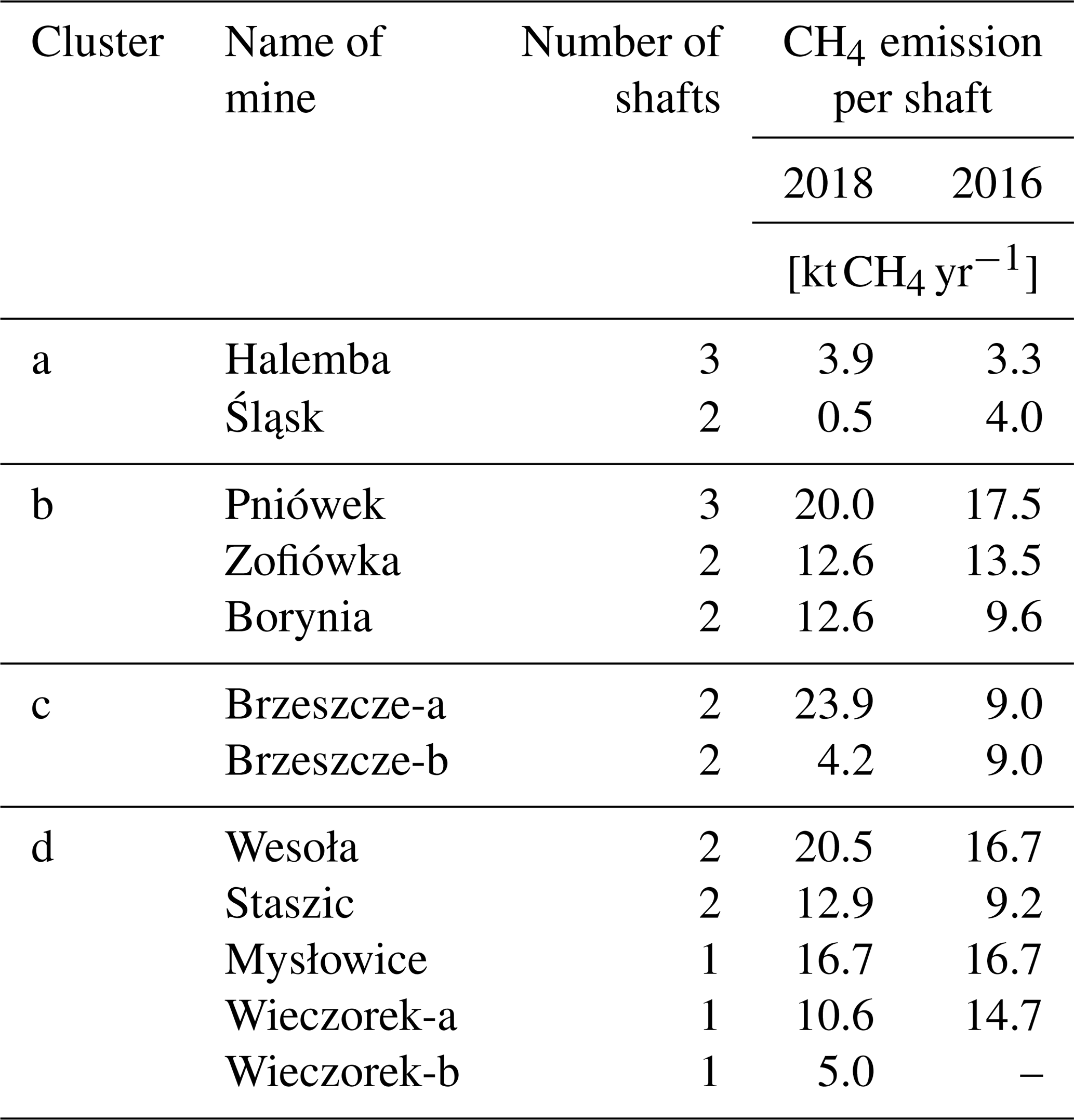
Four clusters of ventilation shafts (Fig. 2) were identified based on the above-mentioned boundary conditions. The clusters are labelled as cluster a to cluster d starting in the north and counting anticlockwise. They comprise ∼40 % of all CH4 mining emissions in the region according to annual emissions from the CoMet ED v4 inventory. The annual CH4 emissions, the name of the mines, and the number of shafts are listed in Table 1. Depending on the position of the flight track, which depends on the prevailing wind direction and cloud cover on a specific day and the air traffic control (ATC) restrictions in that region, not all shafts of a cluster could be covered by each track. This led to the additional investigation of sub-clusters, as discussed further below (Sect. 3.2).
2.4 CoMet ED v4 emission inventory
The core of the CoMet ED v4 inventory (Gałkowski et al., 2021a) comprises annual CH4 emissions, primarily based on data from the European Pollutant Release and Transfer Register (E-PRTR) and the Polish Wyższy Urza̧d Górniczy (WUG, State Mining Authority). As both E-PRTR and the WUG report emissions at the facility level, these had to be disaggregated to individual ventilation shafts. We divided annual emissions equally among the shafts of the reporting mine. Such disaggregation can lead to large uncertainties, since emissions may vary due to changes in excavation activities over the year, related to changes in mining fronts, variations in airflow driven by safety considerations (including methane concentration below ground), etc. The CH4 emissions are displayed for the individual shafts in Fig. 2 for 2018 and listed for the investigated clusters in Table 1 for the years 2016 and 2018.
Table 1Investigated coal mines and their annual CH4 emissions based on the CoMet ED v4 inventory for the year 2018. The values for 2016 are only listed for comparison. The locations of clusters are shown in Fig. 2 and the position of the individual ventilation shafts are marked in the Results section in Figs. 5, C2, C4, and C6.
However, for comparison with instantaneous measurements like ours, emissions with minute or hourly resolution that were measured directly in the investigated shafts at the time of observation should ideally be used. Therefore, we also derived hourly emissions for individual shafts for those coal mines that agreed to provide such information. These data are based on concentrations and airflows measured directly upstream of the outlet of the ventilation shaft. The uncertainty of these hourly emissions is estimated to be 20 % of the reported value due to lacking information about the calibration procedures and instrument precision levels.
3.1 Wind situation over the basin
Overall, the WRF model simulations support the observations by the wind lidars. Exceptions might occur during low-speed wind conditions.

Figure 4Wind situation in the USCB on three different days. Similar to Fig. 2 but complemented by the PBL averaged 2D wind field from the WRF model simulations (black arrows) and the observed wind at the three lidar stations (white arrows). Panel (a) shows favourable and (b) and (c) less favourable wind conditions on 7 June, 1 June, and 29 May, respectively.
Observations from the wind lidar stations are available for all 5 measurement days (28, 29 May and 1, 6, 7 June 2018). Figure 4 illustrates two less favoured and one favourable case. On 7 June between 09:30 and 11:45 LT, the simulated PBL-averaged 2D wind field shows a homogeneous flow from east to west. Additionally, the winds estimated from the three wind lidars (white arrows) agree with the prediction of the model simulation. Similar situations occur for 28 May and 6 June, which also exhibit easterly flows (see Fig. B1). The situation differed on 29 May (Fig. 4c). According to the WRF simulations, the wind speed is significantly lower in some parts of the basin and more variable than on 7 June. The low wind speed is also confirmed by the wind lidars observing winds of around 2 m s−1. Whereas winds from the western lidar (DLR85) appear to agree with the WRF simulations, those from the lidar in the east of the region (DLR86) observe significantly lower wind speeds than predicted by the model (no observations are available for the southern lidar, DLR89, on that day). On 1 June (Fig. 4b), the wind lidars observe a strong gradient in wind speed from west to east with winds blowing from the south-south-east. This is also well captured by the WRF simulations.
During low and variable wind conditions as occurring on 1 June in the south-western basin and also on 29 May, an accumulation or recirculation of the emitted CH4 cannot be excluded. This is less problematic for clusters with few shafts or cases where observations were made close to the shafts. Another limitation results from the cross-sectional flux method introduced in Sect. 2.2.3. The transport through the cross-section described by Eq. (1) must be dominated by advection and not diffusion. For wind speeds slower than 2 m s−1, however, diffusion becomes more prominent (Sharan et al., 1996).
3.2 Estimated cross-sectional fluxes
The following sections present the estimated cross-sectional fluxes and their corresponding errors. Cluster b was investigated during all flights and, consequently, this cluster of shafts has the most comprehensive collection of measurements. It is discussed in more detail below, followed by shorter discussions concerning the three other clusters.
3.2.1 Cluster b
Cluster b comprises seven ventilation shafts from the three mines Pniówek (3), Zofiówka (2), and Borynia (2). They are located in the south-western part of the basin near the Czech border. Their emissions were observed during all six flights, although not all shafts were covered on all days due to the position of the flight tracks.
The wind speeds at cluster b as derived from the lidar stations were generally around 5 to 6 m s−1s and dropped to around 2 m s−1 on 29 May and 1 June. The CH4 column anomalies along the different flight tracks are shown in Fig. 5. In most cases, the wind directions derived from the lidar stations are consistent with the location and extent of the visually observed CH4 column enhancements, representing plumes, and the location of ventilation shaft(s). Reasonable agreement between the wind lidar estimate and the position of the observed plume is even found on 29 May and 1 June, when low and variable winds prevailed. In general, the simulated 2D wind fields match the observed plume(s) and the wind from the wind lidar stations well. The largest differences between model and observations are found on days with low wind speeds according to the wind lidar stations, namely 29 May (Fig. 4b) and 1 June (Fig. 4c), as already identified in Sect. 3.1.

Figure 5WFM-DOAS retrieval results (coloured circles) for CH4 plume(s) originating from shafts in cluster b in the south-western part of the basin during the six different overflights. For visualization only, the anomalies are smoothed by a three-point moving average. The corresponding cross-sectional fluxes are summarized in Table 2, and detailed cross-sections are found in Fig. C1. The grey shading indicates the terrain height, and the border with Czech Republic is represented by the yellow line. Black arrows illustrate the wind field based on WRF model simulations, and red arrows indicate the wind at the position of the cluster/flight track as derived from the three wind lidar stations. Bluish triangles indicate reported annual emissions according to the CoMet ED v4 inventory, and single letters are abbreviations for the ventilation shafts as listed in Table 1 (B: Borynia, Z: Zofiówka, P: Pniówek). Red dots mark the shafts attributed to the observed enhancement. On 7 June, four tracks were acquired; however, two tracks are right on top of each other. The overview map in the lower right corner highlights the investigated area and shafts with a red ellipse.
Table 2Cross-sectional flux estimates for shaft cluster b located in the south-western part of the basin during six different flights and the corresponding winds as derived from the three wind lidar stations (left part). The right part gives the errors of the five components (in %) of the computed flux. The footnote states which mines (number in brackets gives the number of shafts) were investigated. The stated errors of the mean flux (if more than one overflight was available) comprise the uncertainty from the error propagation of the cross-sectional flux method and the track-to-track variability (or atmospheric turbulence) according to Eq. (A4) as discussed in Sect. A2. The last two rows give the annual [kt yr−1] and annually scaled emissions to 1 h [t h−1] of 2018 based on the CoMet ED v4 inventory (Table 1) for comparison with the observed averaged fluxes. For certain shafts, real hourly emissions are available and discussed in Sect. 4.
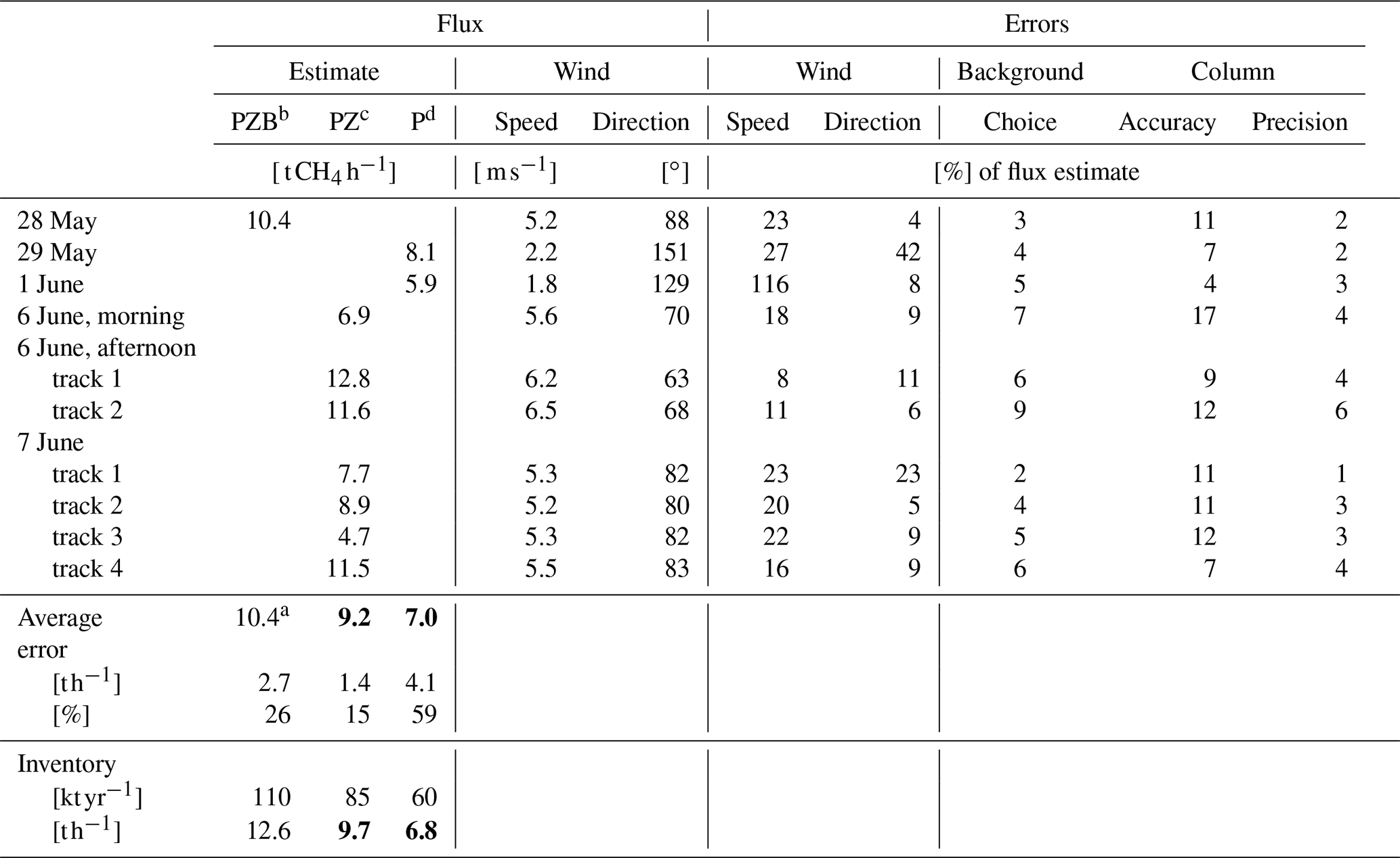
a based on only one single overflight. b Pniówek (3), Zofiówka (2), and Borynia (2). c Pniówek (3), Zofiówka (2). d Pniówek (3).
Only the flight on 28 June covered ventilation shafts from all three mines (sub-cluster PZB). The Pniówek mine alone was investigated on the 2 measurement days with low wind speeds (29 May and 1 June, sub-cluster P), and Pniówek and Zofiówka together were covered on 6 and 7 June (sub-cluster PZ). The individual or single flux estimates and their related uncertainties for cluster b and its sub-clusters are summarized in Table 2 (“single” refers here to the flux of one overflight or track). Most overflights on different days were recorded for the Pniówek and Zofiówka shafts. The single cross-sectional fluxes originating from these two mines with five shafts vary between 4.7 and 12.8 t CH4 h−1 with combined errors (according to Eq. A3) of around 18 % to 34 % on the single fluxes. The error due to variability in the atmospheric transport, which needs to be considered an additional error source for the averaged flux as discussed in Sect. A2, is at the upper end of this range with around 32 % and reduces to 12 % when accounting for the number of flight tracks available (compare Eq. A6). The averaged flux for this sub-cluster is 9.2 t CH4 h−1 with a standard error of 1.4 t CH4 h−1 (or 15 %, calculated according to Eq. A4), which compares well with the reported annual CH4 emission of 9.7 t CH4 h−1. Even for the observations under low-speed wind conditions on 29 May and 1 June (sub-cluster P), the estimated averaged flux agrees with the annual inventory value within 2 %.
As discussed in Sects. 2.2.3 and 2.3, fluxes derived from one single overflight might differ significantly from the true emissions. The flux observed on 28 May is listed for the sake of completeness and should be interpreted with caution, although it agrees with the reported emissions within ∼20 % in this case. A closer look at the inventory values and the observed averaged fluxes is given in Sect. 4.
The dominant error source (Table 2) of the single fluxes is the wind speed (and for some tracks the wind direction) followed by the accuracy of the retrieval and the choice of the background observations. The single-measurement precision of the MAMAP instrument is mostly negligible. The error in the wind speed is usually between 0.5 and 1.2 m s−1, leading to errors in the estimated flux of around 10 % to 25 %, assuming a wind speed of ∼5 m s−1. However, for example, on 1 June the magnitude of the wind was small and variable and its error is larger than the absolute value of 1.8 m s−1. This leads to an error of over 100 % on the single flux estimate and explains the large standard error of more than 50 % on the averaged flux for the Pniówek shafts alone (sub-cluster P).
3.2.2 Clusters a, c, and d
For the remaining clusters, the retrieved CH4 anomalies are shown in Figs. C2, C4, and C6, and the computed cross-sectional fluxes are listed in Table C1. Similar to cluster b, the derived wind directions are consistent with the position of ventilation shafts and the observed plumes. Wind speeds measured by wind lidars were around 5 to 6 m s−1. Exceptions occur again on 29 June and 1 June, when only low-speed and variable winds were encountered, having speeds of between 1.6 to 2.9 m s−1 according to the lidar observations.
Estimated averaged cross-sectional fluxes for clusters a, c, and d range from 1 to ∼8 t CH4 h−1. Similar to cluster b, not all shafts of one cluster could be investigated on all days, leading to a further division into several sub-clusters. Standard errors in the averaged fluxes of each sub-cluster are usually around 20 %. Larger errors occur during low-speed wind conditions (e.g. at sub-cluster WSMW of cluster d with 46 %) or if the fluxes are small and/or only a limited number of overflights are available (e.g. at sub-cluster HS of cluster a with 42 %).
An example, in which the investigation of all ventilation shafts of one cluster is restricted by surface features, is given for cluster c. The flight track is located to the west of four shafts belonging to Brzeszcze on 6 and 7 June (Fig. C4). However, the plume of the northernmost shaft could not be quantitatively investigated, because it was always located directly over an area covered by lakes, which prevent passive remote sensing observations since water surfaces have a very low reflectivity in the SWIR and thus a poor signal-to-noise ratio. During the flight on 1 June, all four shafts were covered. However, only one overflight is available, and the wind speed was low; therefore, the flux is only listed for the sake of completeness.
Since the MAMAP measurements represent a “snapshot” of the emissions of small clusters of ventilation shafts, comparisons to annually resolved and/or coarsely gridded inventories should be treated with care. We do not expect the emissions derived from the observed cross-sectional fluxes to be identical to the reported annual emissions. The reasons for fluctuations in mining emissions are diverse (compare Sects. 1 and 2.4). Some of the measured hourly emissions in the CoMet ED v4 inventory not only indicate fluctuations from hour to hour but also differences between the emissions from different ventilation shafts of one mine. Detailed hourly emission data were, for example, collected for the three Pniówek shafts for the time period between 14 May and 13 June 2018 (see Fig. 6). Maximum hour-to-hour fluctuations reach up to ∼70 % of the average emissions for a single shaft over the 1 month of measurements. For the entire mine, i.e. three shafts combined, fluctuations can still reach ∼30 %. There is no obvious diurnal cycle, but a weekly cycle is found for at least the first part of the time series. Detailed hourly emissions were not only collected for Pniówek but also for the Zofiówka shafts of cluster b (see Table 3).
Table 3Comparison of observed averaged fluxes based on MAMAP data with annually reported emissions and measured averaged hourly emissions, when available. The measured averaged hourly emissions are additionally split into the contributions of the three shafts for Pniówek and two shafts for Zofiówka. See also the main text for further details.
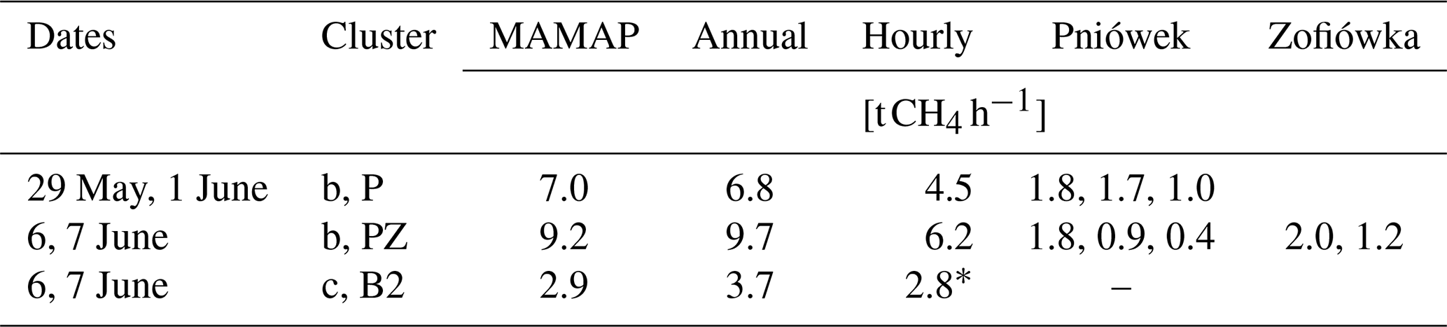
* value is not based on hourly data but partly composed of monthly data between 14 May and 13 June and annual data.
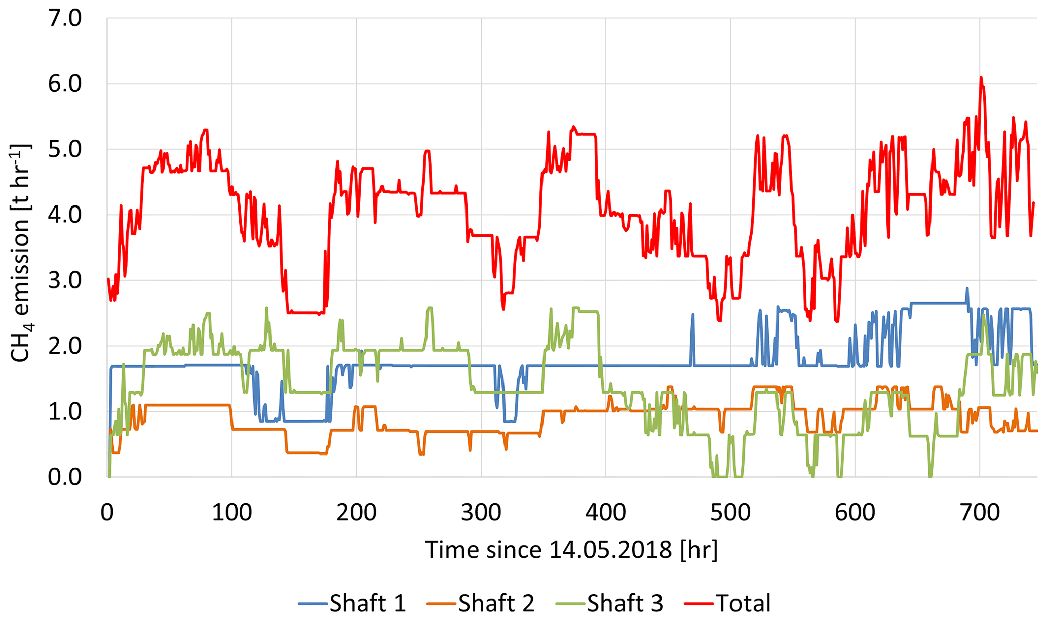
Figure 6Detailed hourly emissions for the three shafts of the Pniówek mine and the entire mine.
For the observations on 29 May and 1 June, where only the Pniówek shafts were investigated and low-speed winds prevailed, the measured averaged hourly emissions for the time of the overflights are 4.5 t CH4 h−1 (∼34 % lower than the reported annual emissions). The term “averaged hourly emissions” refers to the in situ data measured within a shaft according to the CoMet ED v4 inventory. The observed averaged flux derived from MAMAP data is (7.0±4.4) t CH4 h−1. This flux is larger than the measured hourly emissions; however, it was recorded under low-speed wind conditions and is only based on two overflights, both of which call for caution in its interpretation.
The measured averaged hourly emissions for the Pniówek and Zofiówka shafts, which were investigated on 6 and 7 June, are 6.2 t CH4 h−1, which is ∼36 % lower than the annually reported emissions. Although reasonable winds prevailed and seven tracks were acquired in total, the average observed flux based on MAMAP observations is (9.2±1.4) t CH4 h−1 and thus ∼49 % larger than the measured hourly emissions. The mismatch between the observed fluxes and hourly emissions might be related to missing CH4 sources which are not explicitly accounted for in the hourly data. CH4 is, for example, not only ventilated through the ventilation shafts but also drained from excavations and transported to drainage stations in the area. Consequently, CH4 is also released from the drainage system. Those emissions are included in the annually reported emissions but not in the measured hourly data. Additionally, some tracks might also be affected by the two Jastrzebie shafts which are faintly visible in Fig. 5 at around 49.97∘ N, 18.57∘ E. According to the CoMet ED v4 inventory, their annual emissions are reported as 0.3 t CH4 h−1 in total and thus are negligible. However, the measured averaged hourly emissions at the time of the overflights are ∼1 t CH4 h−1 in total, which might influence tracks further downwind. Due to the scatter of the observed fluxes, this effect cannot be investigated further. Taking into account these effects and the standard error of the averaged observed flux derived from MAMAP data (1.4 t CH4 h−1) and the error of the measured hourly emissions (∼1.2 t CH4 h−1 or 20 %), the two values are not significantly different.
For cluster c, which consists of four shafts, the CoMet ED v4 inventory only provides a monthly mean value for the 1-month period between 14 May and 13 June in 2018 for the two high emitting shafts of Brzeszcze-a but no hourly resolved data. The emissions of these shafts are 1.9 and 1.7 t CH4 h−1, which is ∼35 % lower than their reported annual value of 2×2.7 t CH4 h−1 (Table 1). For the two remaining less-active shafts, only the annual emissions of 2×0.5 t CH4 h−1 are available. The investigated sub-cluster B2 of cluster c covers one Brzeszcze-a and the two Brzeszcze-b shafts, resulting in hourly emissions of 2.8 t CH4 h−1 (average of the monthly emissions of the two Brzeszcze-a plus the annually reported value for one Brzeszcze-b shaft), which agrees very well with the observed averaged flux of (2.9±0.5) t CH4 h−1 (Table C1).
For the two remaining clusters a and d, only the annual emissions are available. For cluster a, there is good agreement for the sub-cluster H, consisting of two Halemba shafts (1.0 vs. 0.9 t CH4 h−1, Table C1). However, for the sub-cluster HS, which also includes two Śląsk shafts, the observed averaged flux is larger than the reported annual value by a factor of 3. This might be explained by the limited number of overflights and/or by the variability of the shaft emissions. A similar situation exists for the sub-clusters of cluster d. In the case of favourable wind conditions as for sub-cluster WMW, annually reported emissions and observed average fluxes agree better than for less favourable conditions as for sub-cluster WSMW.
During the CoMet campaign several coal mine ventilation shafts have been investigated by means of passive remote sensing MAMAP and wind lidar observations. The focus was set to small groups of shafts to allow for a better source attribution of the measured CH4 enhancements along the flight tracks and to distinguish emissions from different groups of shafts. In the following, limitations of the applied methods, error sources, and possible improvements are discussed in detail.
Errors of the single fluxes, mainly dominated by the error of the estimated wind speed and direction as well as the retrieved CH4 columns, are between 20 % to 120 % of the respective single flux. Large errors are found, either when the observed flux is relatively low or under low-speed wind conditions. Low fluxes from a weak CH4 source lead to a small signal in the observed CH4 column anomalies, and the error is thus dominated by the instrument's noise or retrieval accuracy. At low wind speeds, the error of the wind speed is as large as the prevailing wind itself. Both error contributors should, however, not be evaluated independently, because the strength of the observed CH4 anomalies inversely depends on wind speed. For the current investigation, wind speeds around 4 to 6 m s−1 with an estimated error of ∼1 m s−1 appear to be optimal, resulting in acceptable wind errors of around 20 % on the single flux with well-detectable CH4 signals in most cases.
Additional errors are caused by the variability of atmospheric transport arising, for example, from turbulence. Depending on the stability of the atmosphere, observed fluxes might vary significantly from flight track to flight track even if the emission strength does not change over time. In the present study, this effect has been approximated by evaluating the standard deviation of all tracks belonging to one sub-cluster. For instance, the error which arises from our current inability to describe turbulence and other molecular mixing, which impact on plume propagation, is estimated to be 30 % of the averaged flux (before accounting for the number of tracks) for the sub-cluster PZ of cluster b. This also means that (1) fluxes based on only one track can significantly deviate from the true flux and should not be considered for evaluation of reported emissions and that (2) further research such as the use of higher-resolution plume modelling is required to better characterize and minimize this source of error.
The errors are significantly reduced by averaging multiple tracks. Under favourable conditions (reasonable winds, multiple flight tracks), the standard error can be reduced to below 20 % of the averaged flux. However, the standard error of the averaged fluxes can also increase to up to 60 % under less favourable conditions (low-speed and variable winds, turbulent atmosphere, few flight tracks, low CH4 emissions).
The calculation of the cross-sectional flux (Eq. 1) implies that a good wind estimate is as important as precise CH4 column anomalies. In the presented study, winds were derived from three wind lidar stations deployed in the USCB. Although the prevailing wind at a specific cluster was interpolated from these stations, the wind direction agrees well with the observed location of CH4 enhancements. Larger discrepancies occur only on days with low and variable winds. On the one hand, this might be attributed to missing wind observations at the southern lidar station on those days. On the other hand, a comparison to WRF v3.9.1.1 model simulations revealed that on those days the wind speed and direction have the largest variability across the basin. We infer that the number of measurements by three stationary wind lidars does not reveal the full complexity of mixing and plume propagation in these conditions. However, modelled wind fields match the wind lidar observations for the remaining days with higher wind speeds. To reflect the effect of a variable wind field across the basin also in the final result, the error of the wind was estimated as 1σ standard deviation of the observed winds at the three lidar stations. This additionally captures the uncertainty related to wind shear and exact vertical distribution of the emission plume within the boundary layer.
An important result of this study is the accurate separation of observed fluxes to specific ventilation shafts or clusters of ventilation shafts. Since the MAMAP instrument observes the total atmospheric air column, fluxes can also be deduced when the emission plume is not entirely mixed vertically within the PBL. This allows the emission to be observed closer to the emission source than it would be sensible with airborne in situ instruments, which generally need to acquire concentration measurements further downwind of a source, where the emissions are well-mixed, to derive reliable fluxes. This comes at the expense of an increased likelihood that plumes from different sources will overlap, making separation difficult. To adequately capture vertical inhomogeneities of emissions in the vicinity of the source by airborne in situ observations, time-consuming dense flight patterns must be carried out, as, for example, described in Conley et al. (2017). However, similar problems also arise with the individual nadir measurements by MAMAP when moving to larger scales due to the large number of wells in this region. In addition, emissions of unknown origin could possibly occur on a larger scale and make interpretation more difficult. In order to clearly assign measured enhancements to sources, imaging instruments are required to observe several pixels across the flight track in one time step and thus create a two-dimensional, gapless map of the anomalies below the aircraft. Examples are the AVIRIS-NG (Thorpe et al., 2017, 2016) and Mako (Tratt et al., 2014) airborne instruments or the MAMAP 2D instrument, which will combine MAMAP's high spectral sampling, sensitivity, and specificity with imaging capability, currently being developed at the Institute of Environmental Physics (IUP), Bremen.
When evaluating MAMAP observations on the scales of clusters of shafts, light path errors must also be taken into account, which would lead to changes in the retrieved CH4 column without any real change in its atmospheric concentration (compare Sects. 2.2.1 and A1). To reduce the light path errors, the CH4 over CO2 proxy method was applied. This method is only valid if the atmospheric CO2 background concentration remains constant during the flight; i.e. there are no significant CO2 sources in the area. On small scales, CO2 sources can be excluded more reliably than on larger scales. Moving to larger scales, CO2 emissions, e.g. from power plants, could alter the observed CH4 anomalies. One solution is to investigate the influence of CO2 inhomogeneities by means of other types of measurements like in situ data as done in Krautwurst et al. (2017). The preferred option is, however, to use a different gas with constant atmospheric concentration for normalization, such as O2 (Schneising et al., 2009; Frankenberg et al., 2006), and to become independent of a homogeneous CO2 background.
Deviations between observed fluxes and reported annual emissions are expected, because the emissions derived from the observed cross-sectional fluxes are only valid for the time of the overflight, and the amount of emitted CH4 and the share between different ventilation shafts vary. Differences in the single cross-sectional fluxes measured on different days, which also capture the variability of the atmospheric transport, might reflect these circumstances. However, due to the large errors in single fluxes, these two effects could not be fully separated. Comparison between hourly emissions and averaged observed fluxes revealed excellent agreement for cluster c and good agreement for cluster b considering the uncertainties and effects discussed in Sect. 4. Comparisons to annually reported emissions of single shafts or small clusters must be handled with caution and are hardly meaningful due to the high variability of the emissions. On larger scales – as, for example, in Fiehn et al. (2020), who analysed airborne in situ observations covering the entire basin – fluctuations of emissions from single shafts or even mines might cancel out.
CH4 emissions from coal mining activities are a significant contributor to anthropogenic greenhouse gas emissions, and their accurate quantification is an essential step to meet the emission reductions agreed on in the Paris Agreement, which is part of the United Nations Framework Convention on Climate Change (UNFCCC, 2015). It addresses greenhouse gas emissions mitigation, adaptation, and finance. Consequently, an important motivation and research question for the multi-instrument and multi-platform campaign CoMet was how well CH4 emissions from one of the largest coal mining areas in Europe can be quantified.
The passive airborne remote sensing instrument MAMAP acquired observations during six flights on 5 measurement days between 28 May and 7 June 2018. The CH4 column anomalies along the flight track were derived using the WFM-DOAS algorithm. These anomalies were combined with estimates of the wind speed and direction from three wind lidar stations, distributed in the USCB as part of the CoMet ground infrastructure, in a mass balance approach to compute cross-sectional fluxes. In total, based on the MAMAP observations, CH4 emissions originating from four clusters comprising 23 ventilation shafts were studied and successfully disentangled. Due to different positions of the flight tracks on different days, smaller groups of shafts from each cluster could be investigated as well. Therefore, the four clusters were split into seven sub-clusters, excluding sub-clusters with only a single overflight, for analysis purposes.
Estimated averaged fluxes range over almost 1 order of magnitude from about 1 to 9 t CH4 h−1 with standard errors of about 15 % to 59 %, whereby fluxes from single overflights of one (sub-)cluster deviated by up to 50 % from the averaged flux. The most important error sources are the accuracy of the CH4 anomaly retrieval of ∼0.10 % relative to the background column, the choice of the background area, and the error in wind speed and wind direction estimated to be ∼1 m s−1 and ∼10∘, respectively, in most cases. In extreme cases, when wind speed and direction were low or variable, the error was as high as the retrieved emission. However, wind speeds were usually around 5 to 6 m s−1, which appears to be a favourable magnitude for estimating reliable fluxes with magnitudes larger than 1 t CH4 h−1. It is recommended that these conditions are targeted during flight planning for future campaigns if remote sensing instruments with a similar sensitivity as that of MAMAP are to be deployed. An additional source of error originated from atmospheric variability due to turbulence or other sources of variation of the atmospheric air flow, preventing flux estimates from single overflights. This error can be reduced by averaging over multiple overflights. Targeting the same emission source more than once should therefore also be an essential part of flight planning activities.
In the USCB region, the emissions of CH4 from ventilation shafts can significantly fluctuate from day to day and even from hour to hour, as discussed in the example of single Pniówek shafts with variations of up to 70 % based on on-site measurements. As a result, observed fluxes could substantially deviate from reported annual values. Therefore, comparison of CH4 fluxes derived from different types of observations requires data acquisition at the same time. Additionally, observed fluxes should only be compared to hourly resolved data to capture the variability correctly. Where hourly data were available, they agreed with the observed fluxes. This emphasizes the need for hourly resolved inventories of anthropogenic emissions to improve top-down and bottom-up comparisons. Overall, the ventilation shafts investigated by MAMAP (excluding shafts only investigated during a single overflight) account for around 40 % of the CH4 mining emissions in the USCB when compared with the annual emissions in the CoMet ED v4 inventory.
Although the 1D MAMAP remote sensing instrument succeeded in estimating emissions of multiple clusters of ventilation shafts, a further breakdown into individual shafts requires a substantial increase in observations. Imaging instruments measuring multiple ground scenes simultaneously during each time step will resolve this issue in the future.
A1 The WFM-DOAS retrieval
A1.1 Algorithm description
For the retrieval of the desired CH4 column anomalies, the WFM-DOAS algorithm (Krings et al., 2011) is applied as introduced in Sect. 2.2.1. It uses simulated radiances, which are representative of the real atmosphere at the time and location of the observation and are compared to the measured spectra. Deviations between the two, which may occur due to enhanced methane in the measurement emitted by a ventilation shaft, are then captured by scaling weighting functions. A weighting function describes the change of radiance due to a change of a selected atmospheric parameter (e.g. changing atmospheric concentrations of CH4 and CO2).
To simulate a reliable background model, i.e. a spectrum which is representative for the real atmosphere, and corresponding weighting functions, the model needs to be provided with several parameters that influence the simulated spectrum. In the case of the MAMAP instrument working between 1590 and 1690 nm, these are primarily vertical concentration profiles of CH4, CO2, and also water vapour (H2O), complemented by pressure and temperature profiles. As backscattered solar radiation from the surface is measured; the spectrum is also influenced by the surface spectral reflectance and by scattering effects from aerosols in the atmosphere. Also geometrical parameters like flight altitude, surface elevation, and solar zenith angle are taken into account.
As these parameters change from flight to flight, they are adapted to the prevailing conditions, and radiative transfer model (RTM) simulations are performed for each flight. Furthermore, a 2D look-up table approach is used to account for strong variations in the light path due to changing surface elevation and solar zenith angle along the flight track. The relevant input parameters are listed in Table A1. The radiances as well as the weighting functions, which are then used as input for the WFM-DOAS retrieval, are calculated by the radiative transfer model SCIATRAN (Rozanov et al., 2014).
Table A1General boundary conditions for the six flights performed during CoMet and also used for the radiative transfer model (RTM) simulations.
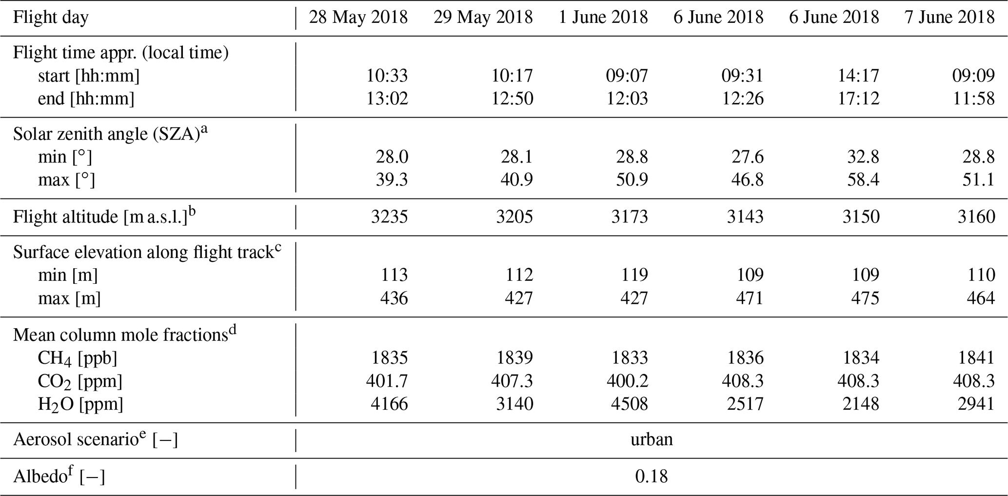
a SZA is computed from the GPS (Global Positioning System) time stamp and assigned to each observation. b Flight altitude is computed as average over the entire flight from the GPS signal. c Topography data are obtained from the Shuttle Radar Topography Mission digital elevation model, which is assigned to each observation based on its current GPS position. In the original work, SRTM Version 2.1 was used; an updated version of this data set can be acquired here: https://search.earthdata.nasa.gov/search?fdc=Shuttle Radar Topography Mission (SRTM)&as[organization][0]=Shuttle Radar Topography Mission (SRTM) (last access: 24 November 2021) (Farr et al., 2007). d The vertical atmospheric profiles are based on the U.S. Standard Atmosphere (USCESA, 1976), which are then adapted according to the airborne in situ observations (CH4 and CO2) acquired by the DLR Cessna, the FUB Cessna, and the DLR HALO as well as the WRF-CHEM v3.9.1.1 model simulations (for H2O). e As aerosol scenario, a standard OPAC (Optical Properties of Aerosol and Clouds; Hess et al., 1998) urban aerosol scenario is applied. f The surface is assumed as a Lambertian reflector with a constant, wavelength-independent surface spectral reflectance in nadir direction of 0.18, which is a common value for midlatitude vegetation and also used in previous studies (e.g. Krings et al., 2011).
The retrieval yields profile scaling factors (PSFs) for the desired trace gas concentrations of CH4 and CO2, from which the CH4 column anomalies are then computed as follows:
with
where is the CH4 column anomaly (in ) used in the cross-sectional flux method (Eq. 1), k is a conversion factor (without units) derived from averaging kernels and takes into account that the sensitivity below the aircraft is around twice as high than above, is the assumed background column of CH4 (in ), and are the retrieved profile scaling factors (without units), and denotes a normalization process with observations from the local background. The formulas including the different quantities are further discussed below.
The retrieved PSFs of CH4 and CO2 describe the relative change in CH4 and CO2 in the measured spectra compared to the simulated one. If the observation was acquired over a CH4 emission plume, the is >1 and the remains 1. However, the PSFs are not only influenced by the respective trace gas concentrations in the atmosphere but also by light path changes resulting from, for example, variations in flight altitude, surface elevation, or enhanced scattering, which is not perfectly covered by the RTM simulations. These light path errors affect the absorption behaviour of both gases in a similar way due to their spectral proximity and can, therefore, be significantly reduced by applying the CH4 over CO2 proxy method (Krings et al., 2013, 2011) denoted by Eq. (A2). The drawback of this method is, however, that strong CO2 sources must not be located in the measurement area, and the CO2 concentration remains constant during one flight, which is true on smaller scales like single shafts or small clusters of shafts but might be invalid if the entire USCB is investigated. Finally, the PSF ratios are normalized by the local background (denoted by in Eq. A1) and corrected by the conversion factor k to get the desired CH4 column anomalies needed for the cross-sectional flux method. The local background is defined similarly to how it has been done in other publications (e.g. Krings et al., 2018; Krautwurst et al., 2017; Frankenberg et al., 2016) as observations outside of a plume in its flanks and determined by visual inspection of each single track downwind of a potential source (cluster).
A1.2 Errors
Errors in the retrieval of the CH4 column anomalies originate from the measurement noise of the instrument or the input parameters for the RTM simulations. The measurement noise is computed as single measurement precision relative to the background column directly from the scatter of the measured data. The retrieval described above is applied and the observations, which are not influenced by a CH4 plume, are used. For the currently investigated data set, this has been estimated to be 0.22 % relative to the background column on average.
Table A2Sensitivity of the retrieved profile scaling factors (PSFs) to the input parameters for the radiative transfer model (RTM) simulations according to expected variations during one flight on 7 June. The deviations for the PSFs of CH4, CO2, and the ratio CH4 to CO2 are again given relative to the background column. The parameters for the true or basic scenario are listed in Table A1, 7 June, using a flight altitude of 3.16 km and a solar zenith angle of 39.4∘. Not all values deviate symmetrically around 0 %; therefore, the worst case scenario is always selected.
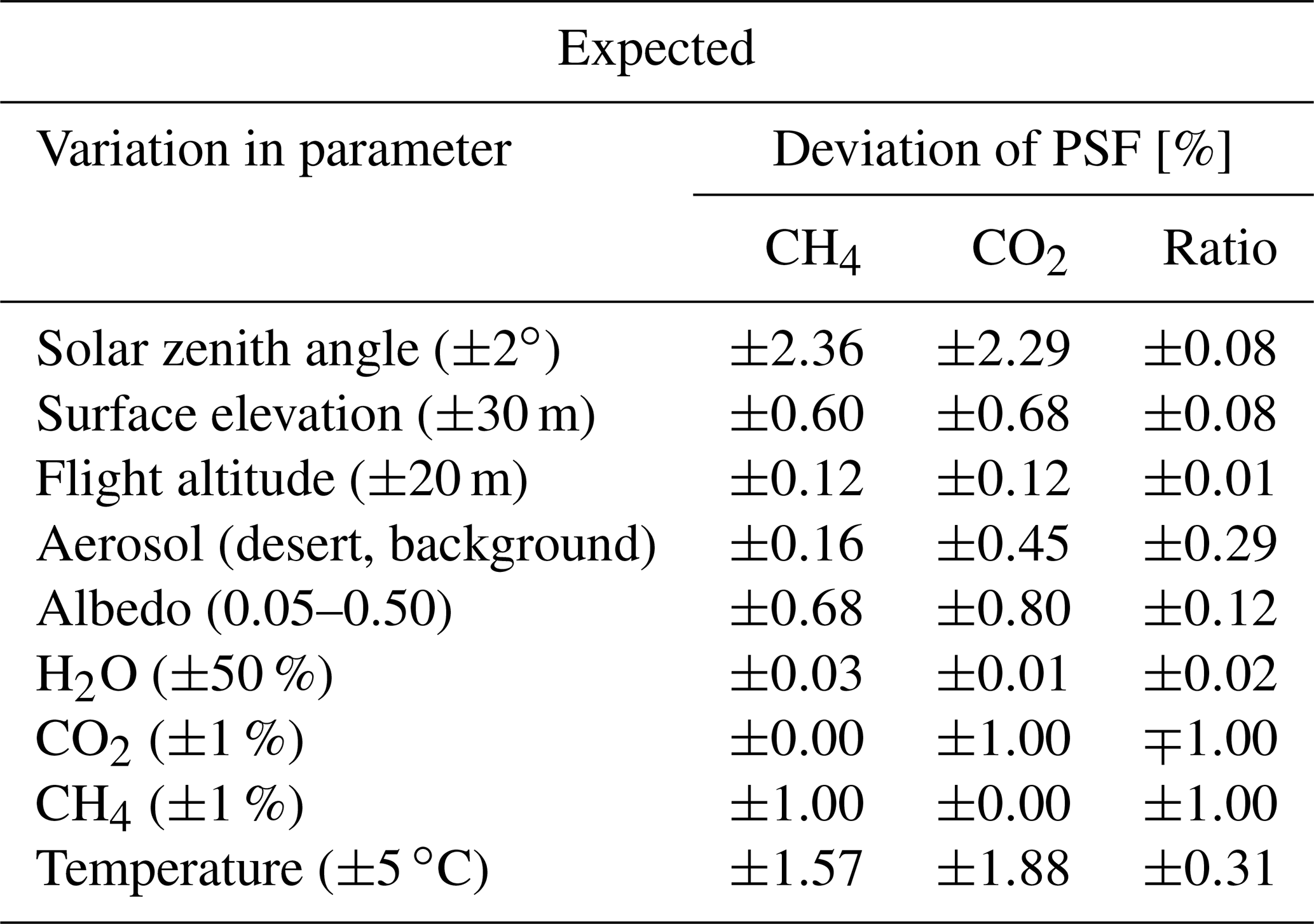
The sensitivity of the input parameters on the final CH4 column anomaly is estimated by using synthetic spectra while varying the input parameters according to their typical variation during a flight as given in Table A2. As expected and already shown in earlier studies (e.g. Krings et al., 2011), the deviations in the fitted profile scaling factors easily reach some percent and, therefore, are on the same order of magnitude as those caused by actual emissions. As most of the deviations are related to light path errors, the applied proxy method reduces these deviations significantly. Most of the remaining effects are systematic and constant along a flight track (e.g. a constant offset caused by wrongly assumed CO2 or CH4 background concentration, background temperature, or background aerosol profiles), and they are corrected by the normalization using observations outside of a plume. Parameters which may not be covered by the normalization process but also do not fluctuate randomly along a flight track and therefore may not be entirely covered by the computed single-measurement precision are surface elevation and surface spectral reflectance. In a worst case scenario, part of the flight track is located over an especially bright surface or over relatively high terrain (forest vs. rangeland) compared to the remaining track. In this study, the uncertainties originating from these two factors are therefore assumed to be uncorrelated and after accounting for the conversion factor k (∼0.69), they potentially lead to a systematic offset of the retrieved CH4 column anomaly of around 0.10 %.
In combination with the single-measurement precision, they are considered in the column anomaly computation by Eq. (1). Although the values in Table A2 are computed for the flight on 7 June, they are assumed to be valid also for the other days.
A2 Errors of the computed fluxes
The error δFtrack of the flux Ftrack of one track is computed by root sum squaring the error sources introduced in Sect. 2.2.3:
where δFu, δFα, δFbg, δFcol-pr, δFcol-ac are the errors arising from the wind speed, from the wind direction, from the choice of the background observations, and from the column anomaly precision and accuracy (in t CH4 h−1). δFu and δFcol-ac are computed by Gaussian error propagation of Eq. (1). δFcol-pr(n) is also calculated by Gaussian error propagation taking into account its random nature by dividing the value for the estimated precision by , where n is the number of observations within the plume. The wind direction modifies the flux via a cosine term, and its error can thus not easily be calculated by error propagation. Consequently, we estimate δFα by varying the prevailing wind direction by its estimated error on a specific day, and we use the difference to the “true” flux Ftrack as error estimate. The choice of the background observations is investigated by randomly selecting two-thirds of the observations from either side of the plume and computing a new background for one flight track, which is used to calculate a new flux estimate. This is done for up to 500 combinations for each side. The 1σ standard deviation of those fluxes is then used to estimate the error δFbg.
An additional uncertainty source originates from variability in the atmospheric transport caused by turbulence and leading to varying cross-sectional fluxes if estimated from multiple overflights of the same source, which cannot be explained by source variability alone (e.g. Wolff et al., 2021; Krautwurst et al., 2017; Matheou and Bowman, 2016). This variability, expressed as δFatm, is estimated as the 1σ standard deviation (SD) from the overflights themselves and is then combined with the error δFtracks, resulting from the errors of the single tracks, to estimate the standard error (1σ) of the averaged flux if multiple overflights of the same source(s) are available:
with
and
where m is the number of flight tracks.
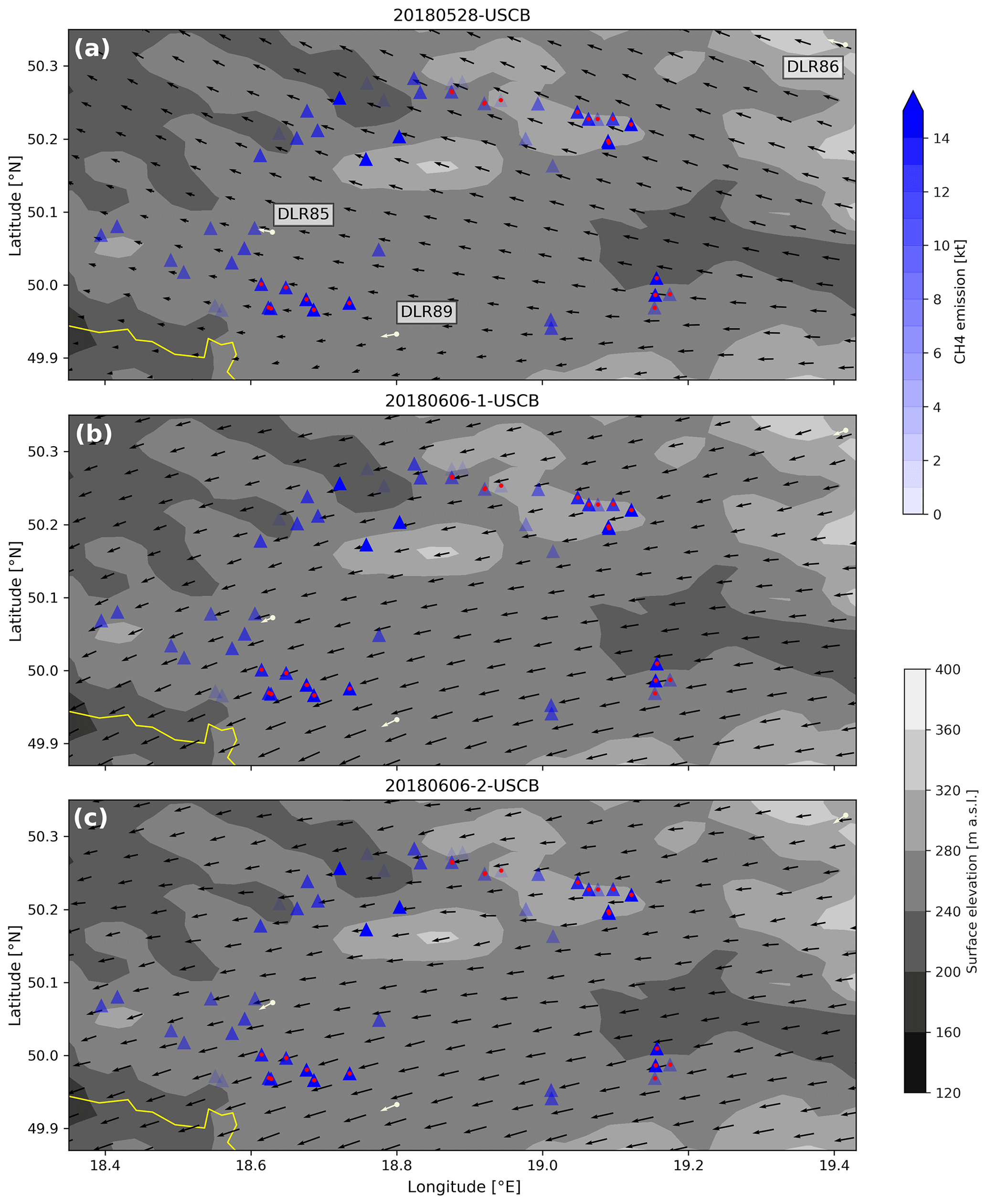
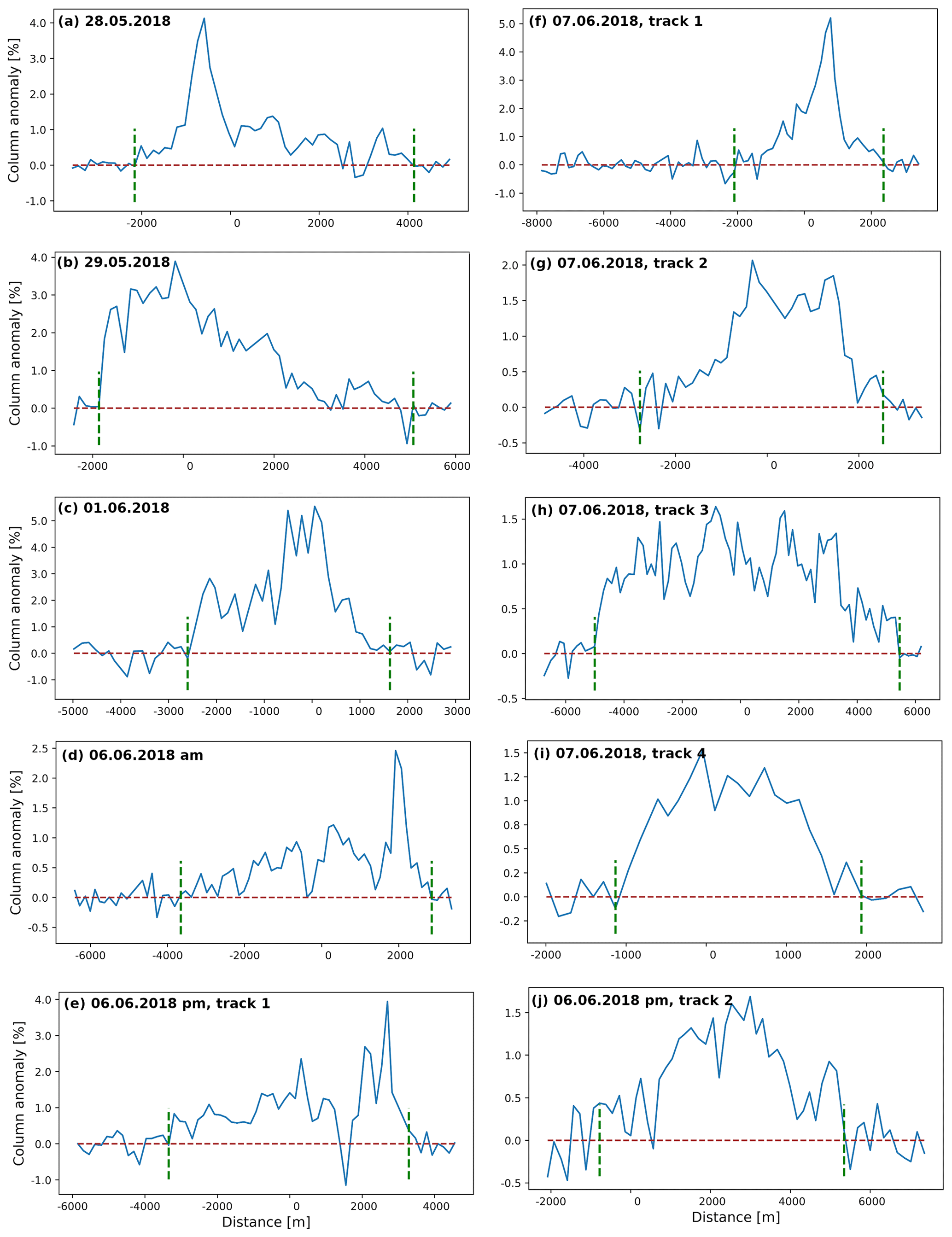
Figure C1CH4 anomalies along the cross-sections downwind of ventilation shafts of cluster b on the different flight days. Green vertical dashed lines separate the plume from the background area. A 2D visualization is shown in Fig. 5.
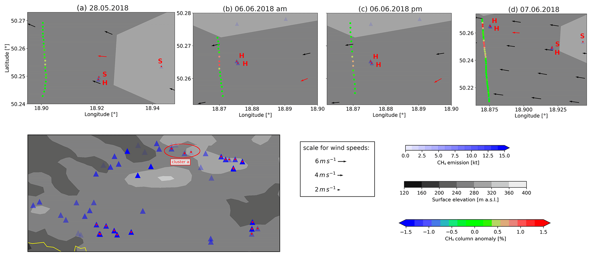
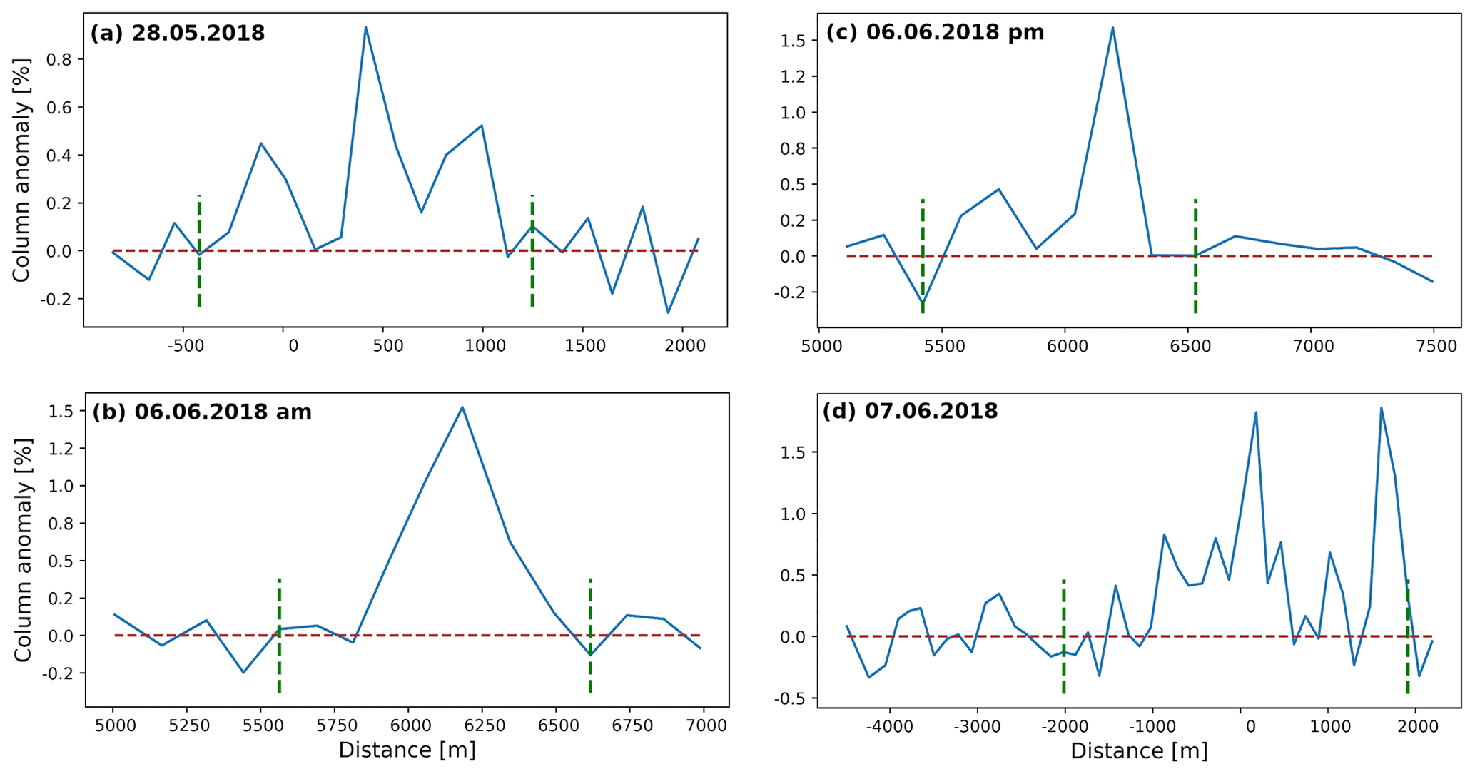

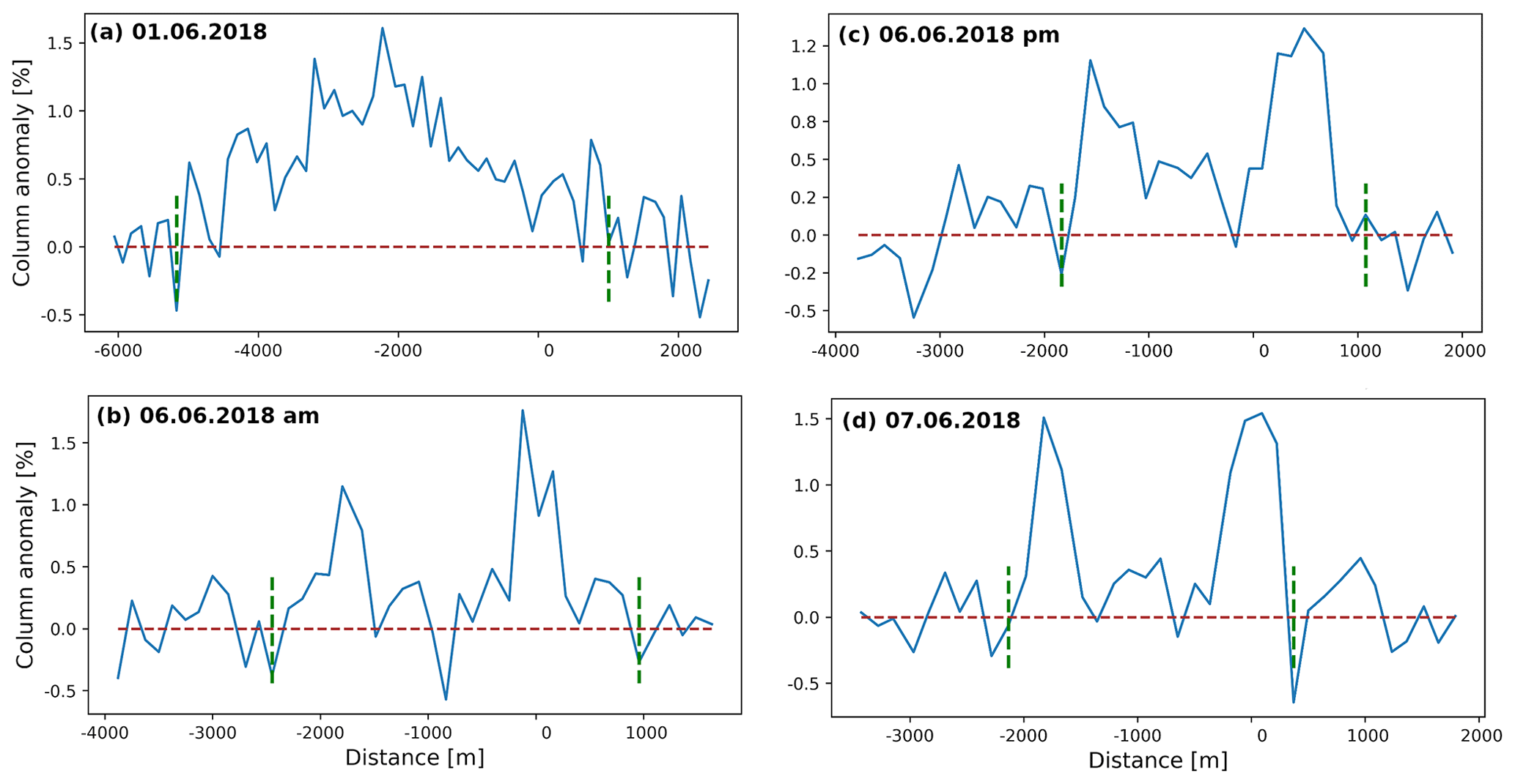
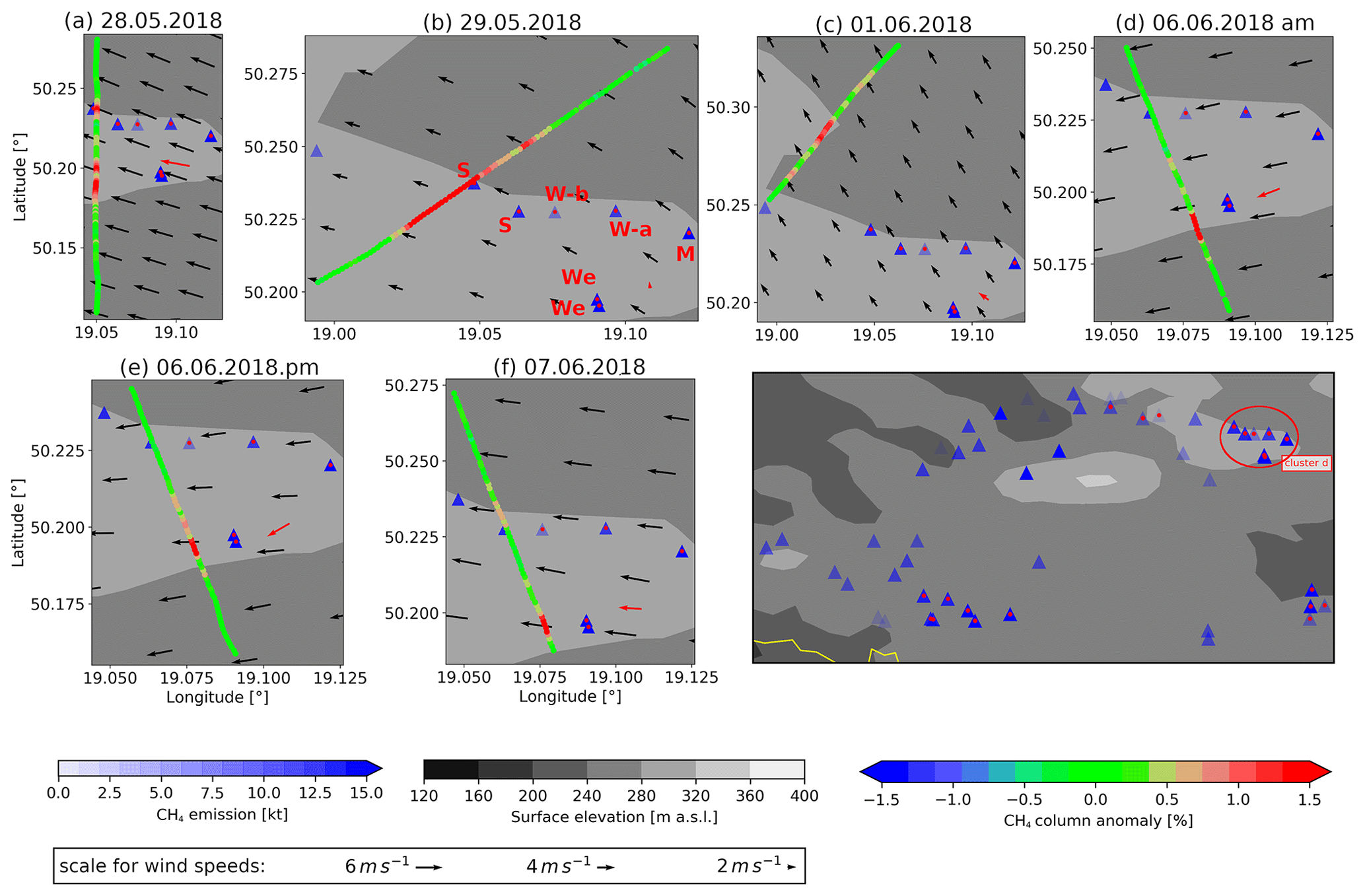
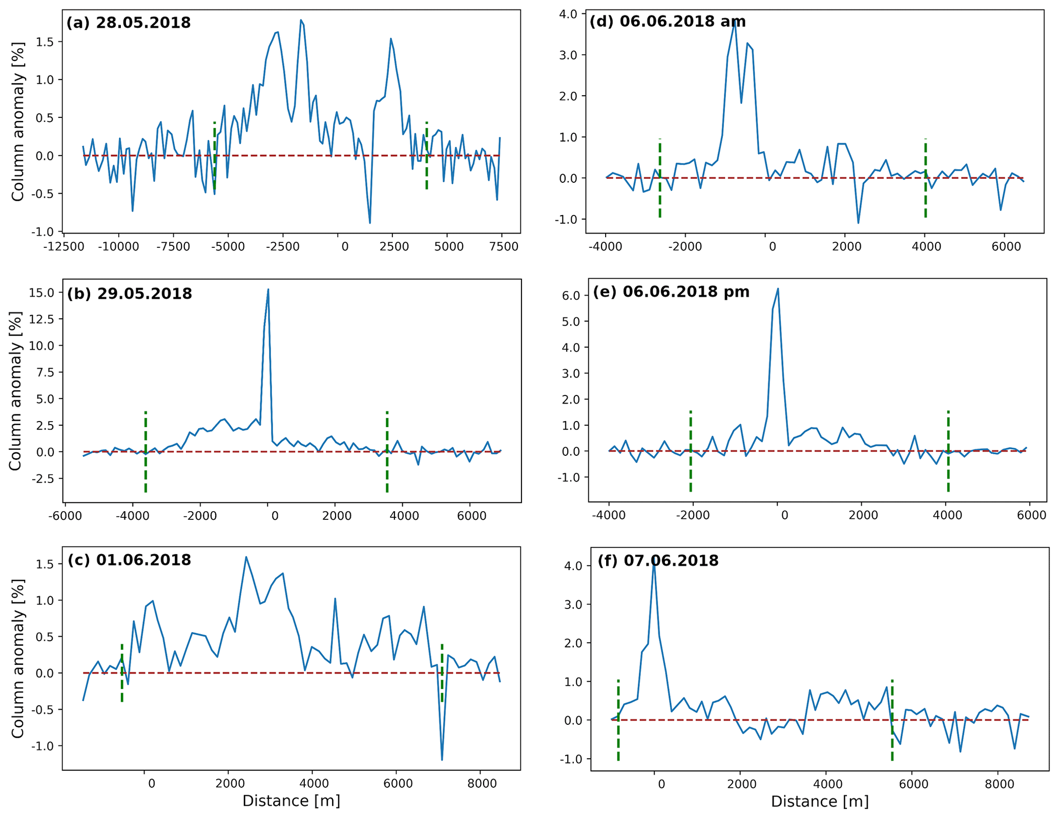
Table C1Same as Table 2 but for clusters a, c, d, and without the errors of the single components.
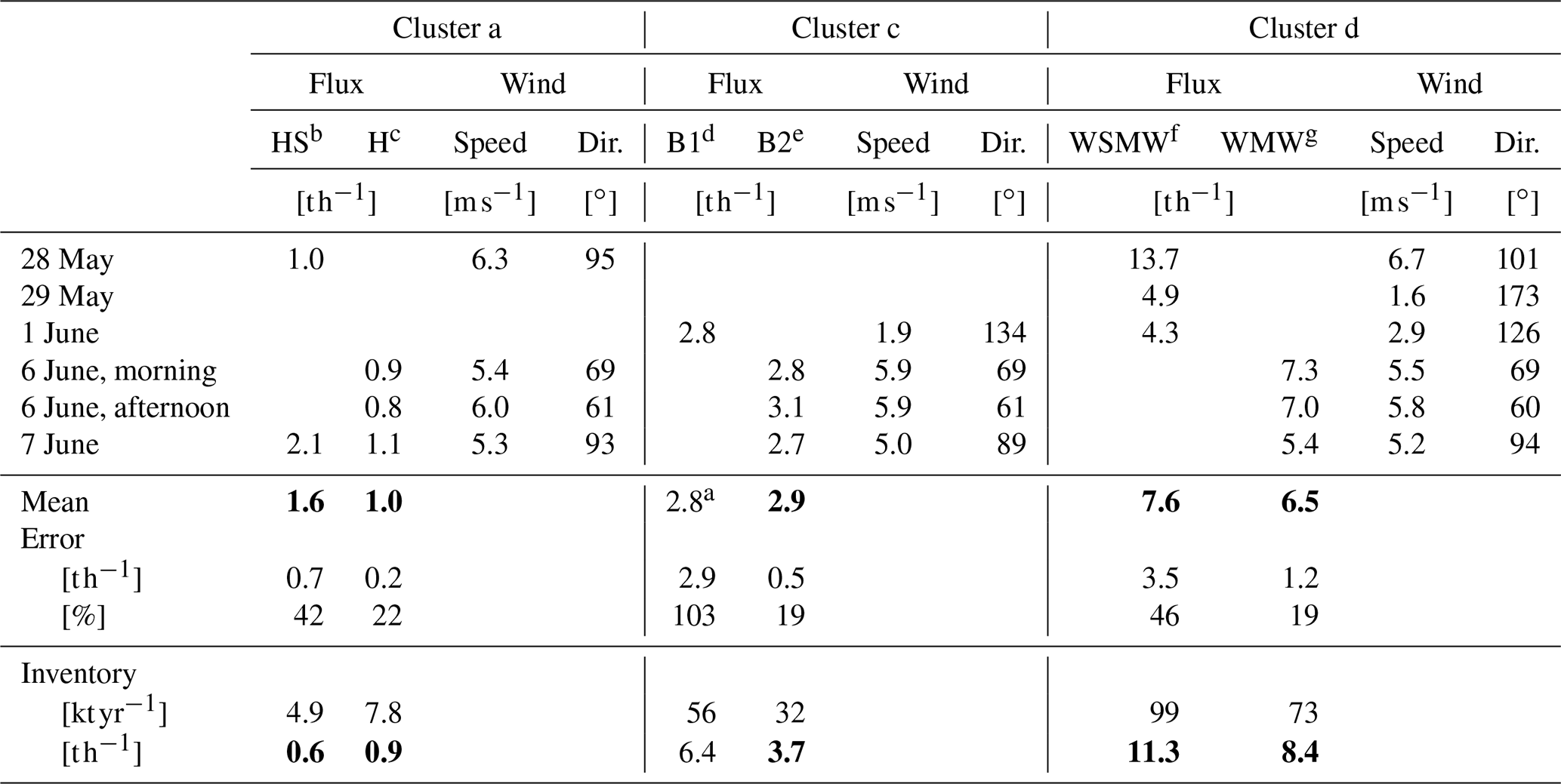
a based on only one single overflight.
b Halemba (1), Śląsk (2).
c Halemba (2). d Brzeszcze-a, -b
(2,2). e Brzeszcze-a, -b (1,2). f Wesoła (2),
Staszic (2), Mysłowice (1), Wieczorek-a, -b (1,1). g Wesoła (2), Mysłowice (1), Wieczorek-a, -b (1,1).
The MAMAP CH4 column anomalies, the observations from the Leosphere WindCube 200S wind lidar systems, and the 3D WRF v3.9.1.1 reanalysis data simulations are available from the authors upon request. The CoMet ED v4 emission inventory can be directly acquired from the ICOS Carbon Portal (https://doi.org/10.18160/3K6Z-4H73, Gałkowski et al., 2021a). The airborne in situ measurements acquired by the DLR Cessna, the FUB Cessna and the DLR HALO can be directly inquired from the authors or can be downloaded from the HALO database (https://halo-db.pa.op.dlr.de/, Deutsches Zentrum für Luft- und Raumfahrt, 2021).
SK processed the remote sensing (RS) data and analysed the RS and wind lidar data as well as data from the WRF-CHEM v3.9.1.1 model simulations, computed the fluxes, and led the writing of the article. KG, JB, HB, and JPB contributed to the paper draft. KG, AnF, HB, and JPB initialized the CoMet activities including the campaign in 2018. SK, KG, JB, MG, AlF, AR, TR, CG, AnF, and HB designed the daily flight plans. SK, KG, and JB collected the remote sensing and in situ data needed for processing of the RS data. MG, AlF, AR, CG, and AnF collected in situ data needed for processing of the RS data. NW collected and processed the wind lidar data. MG and JM performed the WRF-CHEM v3.9.1.1 model simulations. MG, JS, and JN supplied and interpreted data from the CoMet v4 inventory. All authors contributed to the interpretation of the results and the improvement of the article.
The authors declare that they have no conflict of interest.
Publisher's note: Copernicus Publications remains neutral with regard to jurisdictional claims in published maps and institutional affiliations.
This article is part of the special issue “CoMet: a mission to improve our understanding and to better quantify the carbon dioxide and methane cycles”. It is not associated with a conference.
We gratefully acknowledge funding for the CoMet campaign by the BMBF (German Federal Ministry of Education and Research) through AIRSPACE, the State of Bremen, and the MPG (Max Planck Society). The work was further supported by the German Research Foundation (Deutsche Forschungsgemeinschaft, DFG) within the DFG Priority Program (SPP 1294) Atmospheric and Earth System Research with HALO (High Altitude and LOng Range Research Aircraft). We also acknowledge the use of resources of Deutsches Klimarechnungszentrum (DKRZ), namely the high-performance cluster Mistral, for data storage and analysis.
We also gratefully thank Jeremy Gordon, who safely piloted the FUB Cessna during the different flights, and the administration of Katowice Airport, who not only provided us with a parking space for the aircraft and gave us easy access to the hanger to service our measuring instruments during the campaign but also took care of our physical well-being before and after the flights.
This research has been supported by the Bundesministerium für Bildung und Forschung (BMBF) (grant nos. FK 01LK1701B and FK 390 01LK1701C) and the Deutsche Forschungsgemeinschaft (DFG) (grant no. BO 1731/1-1).
The article processing charges for this open-access publication were covered by the University of Bremen.
This paper was edited by Stefano Galmarini and reviewed by four anonymous referees.
Alexe, M., Bergamaschi, P., Segers, A., Detmers, R., Butz, A., Hasekamp, O., Guerlet, S., Parker, R., Boesch, H., Frankenberg, C., Scheepmaker, R. A., Dlugokencky, E., Sweeney, C., Wofsy, S. C., and Kort, E. A.: Inverse modelling of CH4 emissions for 2010–2011 using different satellite retrieval products from GOSAT and SCIAMACHY, Atmos. Chem. Phys., 15, 113–133, https://doi.org/10.5194/acp-15-113-2015, 2015. a
Amediek, A., Ehret, G., Fix, A., Wirth, M., Büdenbender, C., Quatrevalet, M., Kiemle, C., and Gerbig, C.: CHARM-F – a new airborne integrated-path differential-absorption lidar for carbon dioxide and methane observations: measurement performance and quantification of strong point source emissions, Appl. Optics, 56, 5182–5197, https://doi.org/10.1364/AO.56.005182, 2017. a
Buchwitz, M., Schneising, O., Reuter, M., Heymann, J., Krautwurst, S., Bovensmann, H., Burrows, J. P., Boesch, H., Parker, R. J., Somkuti, P., Detmers, R. G., Hasekamp, O. P., Aben, I., Butz, A., Frankenberg, C., and Turner, A. J.: Satellite-derived methane hotspot emission estimates using a fast data-driven method, Atmos. Chem. Phys., 17, 5751–5774, https://doi.org/10.5194/acp-17-5751-2017, 2017. a
Cambaliza, M. O. L., Shepson, P. B., Bogner, J., Caulton, D. R., Stirm, B., Sweeney, C., Montzka, S. A., Gurney, K. R., Spokas, K., Salmon, O. E., Lavoie, T. N., Hendricks, A., Mays, K., Turnbull, J., Miller, B. R., Lauvaux, T., Davis, K., Karion, A., Moser, B., Miller, C., Obermeyer, C., Whetstone, J., Prasad, K., Miles, N., and Richardson, S.: Quantification and source apportionment of the methane emission flux from the city of Indianapolis, Elementa: Science of the Anthropocene, 3, 000037, https://doi.org/10.12952/journal.elementa.000037, 2015. a
Conley, S., Faloona, I., Mehrotra, S., Suard, M., Lenschow, D. H., Sweeney, C., Herndon, S., Schwietzke, S., Pétron, G., Pifer, J., Kort, E. A., and Schnell, R.: Application of Gauss's theorem to quantify localized surface emissions from airborne measurements of wind and trace gases, Atmos. Meas. Tech., 10, 3345–3358, https://doi.org/10.5194/amt-10-3345-2017, 2017. a
Crippa, M., Solazzo, E., Huang, G., Guizzardi, D., Koffi, E., Muntean, M., Schieberle, C., Friedrich, R., and Janssens-Maenhout, G.: High resolution temporal profiles in the Emissions Database for Global Atmospheric Research, Sci. Data, 7, 121, https://doi.org/10.1038/s41597-020-0462-2, 2020. a, b, c
Deutsches Zentrum für Luft- und Raumfahrt: HALO database, available at: https://halo-db.pa.op.dlr.de/, last access: 18 November 2021. a
Dlugokencky, E. J., Nisbet, E. G., Fisher, R., and Lowry, D.: Global atmospheric methane: budget, changes and dangers, Philos. T. R. Soc. S. A, 369, 2058–2072, https://doi.org/10.1098/rsta.2010.0341, 2011. a
EPA: US Environmental Protection Agency: Global Anthropogenic Non-CO2 Greenhouse Gas Emissions: 1990–2030, available at: https://www.epa.gov/global-mitigation-non-co2-greenhouse-gases/global-non-co2-ghg-emissions-1990-2030 (last access: 27 May 2020), 2012. a
Etminan, M., Myhre, G., Highwood, E. J., and Shine, K. P.: Radiative forcing of carbon dioxide, methane, and nitrous oxide: A significant revision of the methane radiative forcing, Geophys. Res. Lett., 43, 12614–12623, https://doi.org/10.1002/2016gl071930, 2016. a, b
Farr, T. G., Rosen, P. A., Caro, E., Crippen, R., Duren, R., Hensley, S., Kobrick, M., Paller, M., Rodriguez, E., Roth, L., Seal, D., Shaffer, S., Shimada, J., Umland, J., Werner, M., Oskin, M., Burbank, D., and Alsdorf, D.: The Shuttle Radar Topography Mission, Rev. Geophys., 45, RG2004, https://doi.org/10.1029/2005RG000183, 2007. a
Fesenfeld, L. P., Schmidt, T. S., and Schrode, A.: Climate policy for short- and long-lived pollutants, Nat. Clim. Change, 8, 933–936, https://doi.org/10.1038/s41558-018-0328-1, 2018. a
Fiehn, A., Kostinek, J., Eckl, M., Klausner, T., Gałkowski, M., Chen, J., Gerbig, C., Röckmann, T., Maazallahi, H., Schmidt, M., Korbeń, P., Neçki, J., Jagoda, P., Wildmann, N., Mallaun, C., Bun, R., Nickl, A.-L., Jöckel, P., Fix, A., and Roiger, A.: Estimating CH4, CO2 and CO emissions from coal mining and industrial activities in the Upper Silesian Coal Basin using an aircraft-based mass balance approach, Atmos. Chem. Phys., 20, 12675–12695, https://doi.org/10.5194/acp-20-12675-2020, 2020. a, b, c
Fix, A. and The CoMet Team: CoMet: An airborne mission to simultaneously measure CO2 and CH4 using lidar, passive remote sensing, and in-situ techniques, Atmos. Meas. Tech., in preparation, 2021. a
Franco, B., Mahieu, E., Emmons, L. K., Tzompa-Sosa, Z. A., Fischer, E. V., Sudo, K., Bovy, B., Conway, S., Griffin, D., Hannigan, J. W., Strong, K., and Walker, K. A.: Evaluating ethane and methane emissions associated with the development of oil and natural gas extraction in North America, Environ. Res. Lett., 11, 044010, https://doi.org/10.1088/1748-9326/11/4/044010, 2016. a
Frankenberg, C., Meirink, J. F., Bergamaschi, P., Goede, A. P. H., Heimann, M., Koerner, S., Platt, U., van Weele, M., and Wagner, T.: Satellite chartography of atmospheric methane from SCIAMACHY on board ENVISAT: Analysis of the years 2003 and 2004, J. Geophys. Res., 111, D07303, https://doi.org/10.1029/2005jd006235, 2006. a
Frankenberg, C., Thorpe, A. K., Thompson, D. R., Hulley, G., Kort, E. A., Vance, N., Borchardt, J., Krings, T., Gerilowski, K., Sweeney, C., Conley, S., Bue, B. D., Aubrey, A. D., Hook, S., and Green, R. O.: Airborne methane remote measurements reveal heavy-tail flux distribution in Four Corners region, P. Natl. Acad. Sci. USA, 113, 9734–9739, https://doi.org/10.1073/pnas.1605617113, 2016. a, b
Gałkowski, M., Fiehn, A., Swolkien, J., Stanisavljevic, M., Korben, P., Menoud, M., Necki, J., Roiger, A., Röckmann, T., Gerbig, C., and Fix, A.: Emissions of CH4 and CO2 over the Upper Silesian Coal Basin (Poland) and its vicinity, ICOS ERIC – Carbon Portal [data set], https://doi.org/10.18160/3K6Z-4H73, 2021a. a, b, c
Gałkowski, M., Jordan, A., Rothe, M., Marshall, J., Koch, F.-T., Chen, J., Agusti-Panareda, A., Fix, A., and Gerbig, C.: In situ observations of greenhouse gases over Europe during the CoMet 1.0 campaign aboard the HALO aircraft, Atmos. Meas. Tech., 14, 1525–1544, https://doi.org/10.5194/amt-14-1525-2021, 2021b. a
Gałkowski, M., Marshall, J., Koch, T., Ho, T.-H., Fix, A., and Gerbig, C.: WRF-GHG Simulations of greenhouse gas distribution over Europe during CoMet Mission, in preparation, 2021c. a, b
Gerilowski, K., Tretner, A., Krings, T., Buchwitz, M., Bertagnolio, P. P., Belemezov, F., Erzinger, J., Burrows, J. P., and Bovensmann, H.: MAMAP – a new spectrometer system for column-averaged methane and carbon dioxide observations from aircraft: instrument description and performance analysis, Atmos. Meas. Tech., 4, 215–243, https://doi.org/10.5194/amt-4-215-2011, 2011. a, b
Gerilowski, K., Krings, T., Hartmann, J., Buchwitz, M., Sachs, T., Erzinger, J., Burrows, J. P., and Bovensmann, H.: Atmospheric remote sensing constraints on direct sea-air methane flux from the 22/4b North Sea massive blowout bubble plume, Mar. Petrol. Geol., 68, 824–835, https://doi.org/10.1016/j.marpetgeo.2015.07.011, 2015. a
Gzyl, G., Janson, E., and Łabaj, P.: Mine Water Discharges in Upper Silesian Coal Basin (Poland), in: Assessment, Restoration and Reclamation of Mining Influenced Soils, Academic Press, 463–486, https://doi.org/10.1016/b978-0-12-809588-1.00017-7, 2017. a
Hausmann, P., Sussmann, R., and Smale, D.: Contribution of oil and natural gas production to renewed increase in atmospheric methane (2007–2014): top–down estimate from ethane and methane column observations, Atmos. Chem. Phys., 16, 3227–3244, https://doi.org/10.5194/acp-16-3227-2016, 2016. a
Helmig, D., Rossabi, S., Hueber, J., Tans, P., Montzka, S. A., Masarie, K., Thoning, K., Plass-Duelmer, C., Claude, A., Carpenter, L. J., Lewis, A. C., Punjabi, S., Reimann, S., Vollmer, M. K., Steinbrecher, R., Hannigan, J. W., Emmons, L. K., Mahieu, E., Franco, B., Smale, D., and Pozzer, A.: Reversal of global atmospheric ethane and propane trends largely due to US oil and natural gas production, Nat. Geosci., 9, 490–495, https://doi.org/10.1038/ngeo2721, 2016. a
Hess, M., Koepke, P., and Schult, I.: Optical properties of aerosols and clouds: The software package OPAC, B. Am. Meteorol. Soc., 79, 831–844, https://doi.org/10.1175/1520-0477(1998)079<0831:OPOAAC>2.0.CO;2, 1998. a
Jackson, R. B., Saunois, M., Bousquet, P., Canadell, J. G., Poulter, B., Stavert, A. R., Bergamaschi, P., Niwa, Y., Segers, A., and Tsuruta, A.: Increasing anthropogenic methane emissions arise equally from agricultural and fossil fuel sources, Environ. Res. Lett., 15, 071002, https://doi.org/10.1088/1748-9326/ab9ed2, 2020. a
Janssens-Maenhout, G., Crippa, M., Guizzardi, D., Muntean, M., Schaaf, E., Dentener, F., Bergamaschi, P., Pagliari, V., Olivier, J. G. J., Peters, J. A. H. W., van Aardenne, J. A., Monni, S., Doering, U., Petrescu, A. M. R., Solazzo, E., and Oreggioni, G. D.: EDGAR v4.3.2 Global Atlas of the three major greenhouse gas emissions for the period 1970–2012, Earth Syst. Sci. Data, 11, 959–1002, https://doi.org/10.5194/essd-11-959-2019, 2019. a, b
Klausner, T., Mertens, M., Huntrieser, H., Gałkowski, M., Kuhlmann, G., Baumann, R., Fiehn, A., Joeckel, P., Puehl, M., Roiger, A., Helmig, D., and Bruhwiler, L.: Urban greenhouse gas emissions from the Berlin area: A case study using airborne CO2 and CH4 in situ observations in summer 2018, Elementa: Science of the Anthropocene, 8, 15, https://doi.org/10.1525/elementa.411, 2020. a
Kostinek, J., Roiger, A., Davis, K. J., Sweeney, C., DiGangi, J. P., Choi, Y., Baier, B., Hase, F., Groß, J., Eckl, M., Klausner, T., and Butz, A.: Adaptation and performance assessment of a quantum and interband cascade laser spectrometer for simultaneous airborne in situ observation of CH4, C2H6, CO2, CO and N2O, Atmos. Meas. Tech., 12, 1767–1783, https://doi.org/10.5194/amt-12-1767-2019, 2019. a
Krautwurst, S., Gerilowski, K., Jonsson, H. H., Thompson, D. R., Kolyer, R. W., Iraci, L. T., Thorpe, A. K., Horstjann, M., Eastwood, M., Leifer, I., Vigil, S. A., Krings, T., Borchardt, J., Buchwitz, M., Fladeland, M. M., Burrows, J. P., and Bovensmann, H.: Methane emissions from a Californian landfill, determined from airborne remote sensing and in situ measurements, Atmos. Meas. Tech., 10, 3429–3452, https://doi.org/10.5194/amt-10-3429-2017, 2017. a, b, c, d, e, f, g
Krings, T., Gerilowski, K., Buchwitz, M., Reuter, M., Tretner, A., Erzinger, J., Heinze, D., Pflüger, U., Burrows, J. P., and Bovensmann, H.: MAMAP – a new spectrometer system for column-averaged methane and carbon dioxide observations from aircraft: retrieval algorithm and first inversions for point source emission rates, Atmos. Meas. Tech., 4, 1735–1758, https://doi.org/10.5194/amt-4-1735-2011, 2011. a, b, c, d, e
Krings, T., Gerilowski, K., Buchwitz, M., Hartmann, J., Sachs, T., Erzinger, J., Burrows, J. P., and Bovensmann, H.: Quantification of methane emission rates from coal mine ventilation shafts using airborne remote sensing data, Atmos. Meas. Tech., 6, 151–166, https://doi.org/10.5194/amt-6-151-2013, 2013. a, b, c
Krings, T., Neininger, B., Gerilowski, K., Krautwurst, S., Buchwitz, M., Burrows, J. P., Lindemann, C., Ruhtz, T., Schüttemeyer, D., and Bovensmann, H.: Airborne remote sensing and in situ measurements of atmospheric CO2 to quantify point source emissions, Atmos. Meas. Tech., 11, 721–739, https://doi.org/10.5194/amt-11-721-2018, 2018. a, b
Lavoie, T. N., Shepson, P. B., Cambaliza, M. O. L., Stirm, B. H., Karion, A., Sweeney, C., Yacovitch, T. I., Herndon, S. C., Lan, X., and Lyon, D.: Aircraft-Based Measurements of Point Source Methane Emissions in the Barnett Shale Basin, Environ. Sci. Technol., 49, 7904–7913, https://doi.org/10.1021/acs.est.5b00410, 2015. a
Luther, A., Kleinschek, R., Scheidweiler, L., Defratyka, S., Stanisavljevic, M., Forstmaier, A., Dandocsi, A., Wolff, S., Dubravica, D., Wildmann, N., Kostinek, J., Jöckel, P., Nickl, A.-L., Klausner, T., Hase, F., Frey, M., Chen, J., Dietrich, F., Neçcki, J., Swolkień, J., Fix, A., Roiger, A., and Butz, A.: Quantifying CH4 emissions from hard coal mines using mobile sun-viewing Fourier transform spectrometry, Atmos. Meas. Tech., 12, 5217–5230, https://doi.org/10.5194/amt-12-5217-2019, 2019. a, b, c
Maasakkers, J. D., Jacob, D. J., Sulprizio, M. P., Turner, A. J., Weitz, M., Wirth, T., Hight, C., DeFigueiredo, M., Desai, M., Schmeltz, R., Hockstad, L., Bloom, A. A., Bowman, K. W., Jeong, S., and Fischer, M. L.: Gridded National Inventory of U. S. Methane Emissions, Environ. Sci. Technol., 50, 13123–13133, https://doi.org/10.1021/acs.est.6b02878, 2016. a
Matheou, G. and Bowman, K. W.: A recycling method for the large-eddy simulation of plumes in the atmospheric boundary layer, Environ. Fluid Mech., 16, 69–85, https://doi.org/10.1007/s10652-015-9413-4, 2016. a
Myhre, G., Shindell, D., Breon, F.-M., Collins, W., Fuglestvedt, J., Huang, J., Koch, D., Lamarque, J.-F., Lee, D., Mendoza, B., Nakajima, T., Robock, A., Stephens, G., Takemura, T., and Zhang, H.: Anthropogenic and Natural Radiative Forcing, book section 8, Cambridge University Press, Cambridge, UK and New York, NY, USA, 659–740, https://doi.org/10.1017/CBO9781107415324.018, 2013. a, b
Nickl, A.-L., Mertens, M., Roiger, A., Fix, A., Amediek, A., Fiehn, A., Gerbig, C., Gałkowski, M., Kerkweg, A., Klausner, T., Eckl, M., and Jöckel, P.: Hindcasting and forecasting of regional methane from coal mine emissions in the Upper Silesian Coal Basin using the online nested global regional chemistry–climate model MECO(n) (MESSy v2.53), Geosci. Model Dev., 13, 1925–1943, https://doi.org/10.5194/gmd-13-1925-2020, 2020. a, b
Nisbet, E. G., Dlugokencky, E. J., Manning, M. R., Lowry, D., Fisher, R. E., France, J. L., Michel, S. E., Miller, J. B., White, J. W. C., Vaughn, B., Bousquet, P., Pyle, J. A., Warwick, N. J., Cain, M., Brownlow, R., Zazzeri, G., Lanoisellé, M., Manning, A. C., Gloor, E., Worthy, D. E. J., Brunke, E.-G., Labuschagne, C., Wolff, E. W., and Ganesan, A. L.: Rising atmospheric methane: 2007–2014 growth and isotopic shift, Global Biogeochem. Cy., 30, 1356–1370, https://doi.org/10.1002/2016gb005406, 2016. a
Peischl, J., Karion, A., Sweeney, C., Kort, E. A., Smith, M. L., Brandt, A. R., Yeskoo, T., Aikin, K. C., Conley, S. A., Gvakharia, A., Trainer, M., Wolter, S., and Ryerson, T. B.: Quantifying atmospheric methane emissions from oil and natural gas production in the Bakken shale region of North Dakota, J. Geophys. Res.-Atmos., 121, 6101–6111, https://doi.org/10.1002/2015jd024631, 2016. a
Petrenko, V. V., Smith, A. M., Schaefer, H., Riedel, K., Brook, E., Baggenstos, D., Harth, C., Hua, Q., Buizert, C., Schilt, A., Fain, X., Mitchell, L., Bauska, T., Orsi, A., Weiss, R. F., and Severinghaus, J. P.: Minimal geological methane emissions during the Younger Dryas–Preboreal abrupt warming event, Nature, 548, 443–446, https://doi.org/10.1038/nature23316, 2017. a
Prather, M. J., Holmes, C. D., and Hsu, J.: Reactive greenhouse gas scenarios: Systematic exploration of uncertainties and the role of atmospheric chemistry, Geophys. Res. Lett., 39, L09803, https://doi.org/10.1029/2012gl051440, 2012. a
Reuter, M., Buchwitz, M., Schneising, O., Krautwurst, S., O'Dell, C. W., Richter, A., Bovensmann, H., and Burrows, J. P.: Towards monitoring localized CO2 emissions from space: co-located regional CO2 and NO2 enhancements observed by the OCO-2 and S5P satellites, Atmos. Chem. Phys., 19, 9371–9383, https://doi.org/10.5194/acp-19-9371-2019, 2019. a
Rigby, M., Montzka, S. A., Prinn, R. G., White, J. W. C., Young, D., ODoherty, S., Lunt, M. F., Ganesan, A. L., Manning, A. J., Simmonds, P. G., Salameh, P. K., Harth, C. M., Muehle, J., Weiss, R. F., Fraser, P. J., Steele, L. P., Krummel, P. B., McCulloch, A., and Park, S.: Role of atmospheric oxidation in recent methane growth, P. Natl. Acad. Sci. USA, 114, 5373–5377, https://doi.org/10.1073/pnas.1616426114, 2017. a
Rozanov, V., Rozanov, A., Kokhanovsky, A., and Burrows, J.: Radiative transfer through terrestrial atmosphere and ocean: Software package SCIATRAN, J. Quant. Spectrosc. Ra., 133, 13–71, https://doi.org/10.1016/j.jqsrt.2013.07.004, 2014. a
Saunois, M., Bousquet, P., Poulter, B., Peregon, A., Ciais, P., Canadell, J. G., Dlugokencky, E. J., Etiope, G., Bastviken, D., Houweling, S., Janssens-Maenhout, G., Tubiello, F. N., Castaldi, S., Jackson, R. B., Alexe, M., Arora, V. K., Beerling, D. J., Bergamaschi, P., Blake, D. R., Brailsford, G., Brovkin, V., Bruhwiler, L., Crevoisier, C., Crill, P., Covey, K., Curry, C., Frankenberg, C., Gedney, N., Höglund-Isaksson, L., Ishizawa, M., Ito, A., Joos, F., Kim, H.-S., Kleinen, T., Krummel, P., Lamarque, J.-F., Langenfelds, R., Locatelli, R., Machida, T., Maksyutov, S., McDonald, K. C., Marshall, J., Melton, J. R., Morino, I., Naik, V., O'Doherty, S., Parmentier, F.-J. W., Patra, P. K., Peng, C., Peng, S., Peters, G. P., Pison, I., Prigent, C., Prinn, R., Ramonet, M., Riley, W. J., Saito, M., Santini, M., Schroeder, R., Simpson, I. J., Spahni, R., Steele, P., Takizawa, A., Thornton, B. F., Tian, H., Tohjima, Y., Viovy, N., Voulgarakis, A., van Weele, M., van der Werf, G. R., Weiss, R., Wiedinmyer, C., Wilton, D. J., Wiltshire, A., Worthy, D., Wunch, D., Xu, X., Yoshida, Y., Zhang, B., Zhang, Z., and Zhu, Q.: The global methane budget 2000–2012, Earth Syst. Sci. Data, 8, 697–751, https://doi.org/10.5194/essd-8-697-2016, 2016. a, b, c
Saunois, M., Stavert, A. R., Poulter, B., Bousquet, P., Canadell, J. G., Jackson, R. B., Raymond, P. A., Dlugokencky, E. J., Houweling, S., Patra, P. K., Ciais, P., Arora, V. K., Bastviken, D., Bergamaschi, P., Blake, D. R., Brailsford, G., Bruhwiler, L., Carlson, K. M., Carrol, M., Castaldi, S., Chandra, N., Crevoisier, C., Crill, P. M., Covey, K., Curry, C. L., Etiope, G., Frankenberg, C., Gedney, N., Hegglin, M. I., Höglund-Isaksson, L., Hugelius, G., Ishizawa, M., Ito, A., Janssens-Maenhout, G., Jensen, K. M., Joos, F., Kleinen, T., Krummel, P. B., Langenfelds, R. L., Laruelle, G. G., Liu, L., Machida, T., Maksyutov, S., McDonald, K. C., McNorton, J., Miller, P. A., Melton, J. R., Morino, I., Müller, J., Murguia-Flores, F., Naik, V., Niwa, Y., Noce, S., O'Doherty, S., Parker, R. J., Peng, C., Peng, S., Peters, G. P., Prigent, C., Prinn, R., Ramonet, M., Regnier, P., Riley, W. J., Rosentreter, J. A., Segers, A., Simpson, I. J., Shi, H., Smith, S. J., Steele, L. P., Thornton, B. F., Tian, H., Tohjima, Y., Tubiello, F. N., Tsuruta, A., Viovy, N., Voulgarakis, A., Weber, T. S., van Weele, M., van der Werf, G. R., Weiss, R. F., Worthy, D., Wunch, D., Yin, Y., Yoshida, Y., Zhang, W., Zhang, Z., Zhao, Y., Zheng, B., Zhu, Q., Zhu, Q., and Zhuang, Q.: The Global Methane Budget 2000–2017, Earth Syst. Sci. Data, 12, 1561–1623, https://doi.org/10.5194/essd-12-1561-2020, 2020. a
Scarpelli, T. R., Jacob, D. J., Maasakkers, J. D., Sulprizio, M. P., Sheng, J.-X., Rose, K., Romeo, L., Worden, J. R., and Janssens-Maenhout, G.: A global gridded () inventory of methane emissions from oil, gas, and coal exploitation based on national reports to the United Nations Framework Convention on Climate Change, Earth Syst. Sci. Data, 12, 563–575, https://doi.org/10.5194/essd-12-563-2020, 2020. a, b, c, d
Schaefer, H., Fletcher, S. E. M., Veidt, C., Lassey, K. R., Brailsford, G. W., Bromley, T. M., Dlugokencky, E. J., Michel, S. E., Miller, J. B., Levin, I., Lowe, D. C., Martin, R. J., Vaughn, B. H., and White, J. W. C.: A 21st-century shift from fossil-fuel to biogenic methane emissions indicated by 13CH4, Science, 352, 80–84, https://doi.org/10.1126/science.aad2705, 2016. a
Schneising, O., Buchwitz, M., Burrows, J. P., Bovensmann, H., Bergamaschi, P., and Peters, W.: Three years of greenhouse gas column-averaged dry air mole fractions retrieved from satellite – Part 2: Methane, Atmos. Chem. Phys., 9, 443–465, https://doi.org/10.5194/acp-9-443-2009, 2009. a
Schwietzke, S., Sherwood, O. A., Bruhwiler, L. M. P., Miller, J. B., Etiope, G., Dlugokencky, E. J., Michel, S. E., Arling, V. A., Vaughn, B. H., White, J. W. C., and Tans, P. P.: Upward revision of global fossil fuel methane emissions based on isotope database, Nature, 538, 88–91, https://doi.org/10.1038/nature19797, 2016. a, b
Sharan, M., Yadav, A. K., Singh, M., Agarwal, P., and Nigam, S.: A mathematical model for the dispersion of air pollutants in low wind conditions, Atmos. Environ., 30, 1209–1220, https://doi.org/10.1016/1352-2310(95)00442-4, 1996. a
Shindell, D., Kuylenstierna, J. C. I., Vignati, E., van Dingenen, R., Amann, M., Klimont, Z., Anenberg, S. C., Muller, N., Janssens-Maenhout, G., Raes, F., Schwartz, J., Faluvegi, G., Pozzoli, L., Kupiainen, K., Hoeglund-Isaksson, L., Emberson, L., Streets, D., Ramanathan, V., Hicks, K., Oanh, N. T. K., Milly, G., Williams, M., Demkine, V., and Fowler, D.: Simultaneously Mitigating Near-Term Climate Change and Improving Human Health and Food Security, Science, 335, 183–189, https://doi.org/10.1126/science.1210026, 2012. a
Smalikho, I.: Techniques of Wind Vector Estimation from Data Measured with a Scanning Coherent Doppler Lidar, J. Atmos. Ocean. Tech., 20, 276–291, https://doi.org/10.1175/1520-0426(2003)020<0276:towvef>2.0.co;2, 2003. a
Smalikho, I. N. and Banakh, V. A.: Measurements of wind turbulence parameters by a conically scanning coherent Doppler lidar in the atmospheric boundary layer, Atmos. Meas. Tech., 10, 4191–4208, https://doi.org/10.5194/amt-10-4191-2017, 2017. a
Stephan, A., Smalikho, I. N., and Wildmann, N.: Effectiveness of the MFAS method for retrieval of height profiles of speed and direction of the wind from measurements by a Windcube 200s lidar, in: 24th International Symposium on Atmospheric and Ocean Optics: Atmospheric Physics, edited by: Romanovskii, O. A. and Matvienko, G. G., SPIE, 2–5 July 2018, Tomsk, Russian Federation, https://doi.org/10.1117/12.2504450, 2018a. a
Stephan, A., Smalikho, I. N., and Wildmann, N.: Spatiotemporal visualization of wind turbulence from measurements by a Windcube 200s lidar in the atmospheric boundary layer, in: 24th International Symposium on Atmospheric and Ocean Optics: Atmospheric Physics, edited by: Romanovskii, O. A. and Matvienko, G. G., SPIE, 2–5 July 2018, Tomsk, Russian Federation, https://doi.org/10.1117/12.2504468, 2018b. a
Stocker, T., Qin, D., Plattner, G.-K., Alexander, L., Allen, S., Bindoff, N., Breon, F.-M., Church, J., Cubasch, U., Emori, S., Forster, P., Friedlingstein, P., Gillett, N., Gregory, J., Hartmann, D., Jansen, E., Kirtman, B., Knutti, R., Krishna Kumar, K., Lemke, P., Marotzke, J., Masson-Delmotte, V., Meehl, G., Mokhov, I., Piao, S., Ramaswamy, V., Randall, D., Rhein, M., Rojas, M., Sabine, C., Shindell, D., Talley, L., Vaughan, D., and Xie, S.-P.: Technical Summary, book section TS, Cambridge University Press, Cambridge, UK and New York, NY, USA, 33–115, https://doi.org/10.1017/CBO9781107415324.005, 2013. a
Swolkien, J., Fix, A., and Gałkowski, M.: Factors that influence the temporal variability of atmospheric methane emission from Upper Silesia coal mines: A case study from CoMet mission, in preparation, 2021. a
Thorpe, A. K., Frankenberg, C., Aubrey, A. D., Roberts, D. A., Nottrott, A. A., Rahn, T. A., Sauer, J. A., Dubey, M. K., Costigan, K. R., Arata, C., Steffke, A. M., Hills, S., Haselwimmer, C., Charlesworth, D., Funk, C. C., Green, R. O., Lundeen, S. R., Boardman, J. W., Eastwood, M. L., Sarture, C. M., Nolte, S. H., Mccubbin, I. B., Thompson, D. R., and McFadden, J. P.: Mapping methane concentrations from a controlled release experiment using the next generation airborne visible/infrared imaging spectrometer (AVIRIS-NG), Remote Sens. Environ., 179, 104–115, https://doi.org/10.1016/j.rse.2016.03.032, 2016. a
Thorpe, A. K., Frankenberg, C., Thompson, D. R., Duren, R. M., Aubrey, A. D., Bue, B. D., Green, R. O., Gerilowski, K., Krings, T., Borchardt, J., Kort, E. A., Sweeney, C., Conley, S., Roberts, D. A., and Dennison, P. E.: Airborne DOAS retrievals of methane, carbon dioxide, and water vapor concentrations at high spatial resolution: application to AVIRIS-NG, Atmos. Meas. Tech., 10, 3833–3850, https://doi.org/10.5194/amt-10-3833-2017, 2017. a
Tratt, D. M., Buckland, K. N., Hall, J. L., Johnson, P. D., Keim, E. R., Leifer, I., Westberg, K., and Young, S. J.: Airborne visualization and quantification of discrete methane sources in the environment, Remote Sens. Environ., 154, 74–88, https://doi.org/10.1016/j.rse.2014.08.011, 2014. a
Turnbull, J. C., Karion, A., Fischer, M. L., Faloona, I., Guilderson, T., Lehman, S. J., Miller, B. R., Miller, J. B., Montzka, S., Sherwood, T., Saripalli, S., Sweeney, C., and Tans, P. P.: Assessment of fossil fuel carbon dioxide and other anthropogenic trace gas emissions from airborne measurements over Sacramento, California in spring 2009, Atmos. Chem. Phys., 11, 705–721, https://doi.org/10.5194/acp-11-705-2011, 2011. a
Turner, A. J., Jacob, D. J., Wecht, K. J., Maasakkers, J. D., Lundgren, E., Andrews, A. E., Biraud, S. C., Boesch, H., Bowman, K. W., Deutscher, N. M., Dubey, M. K., Griffith, D. W. T., Hase, F., Kuze, A., Notholt, J., Ohyama, H., Parker, R., Payne, V. H., Sussmann, R., Sweeney, C., Velazco, V. A., Warneke, T., Wennberg, P. O., and Wunch, D.: Estimating global and North American methane emissions with high spatial resolution using GOSAT satellite data, Atmos. Chem. Phys., 15, 7049–7069, https://doi.org/10.5194/acp-15-7049-2015, 2015. a
Turner, A. J., Jacob, D. J., Benmergui, J., Wofsy, S. C., Maasakkers, J. D., Butz, A., Hasekamp, O., and Biraud, S. C.: A large increase in U. S. methane emissions over the past decade inferred from satellite data and surface observations, Geophys. Res. Lett., 43, 2218–2224, https://doi.org/10.1002/2016gl067987, 2016. a
Turner, A. J., Frankenberg, C., Wennberg, P. O., and Jacob, D. J.: Ambiguity in the causes for decadal trends in atmospheric methane and hydroxyl, P. Natl. Acad. Sci. USA, 114, 5367–5372, https://doi.org/10.1073/pnas.1616020114, 2017. a
UNFCCC: United Nations Framework Convention on Climate Change: Kyoto Protocol to the United Nations Framework Convention on Climate Change, available at: http://unfccc.int/kyoto_protocol/items/2830.php (last access: 7 November 2017), 1998. a
UNFCCC: United Nations Framework Convention on Climate Change: The Paris Agreement, COP21 (Decision: 1/C P.21), available at: http://unfccc.int/paris_agreement/items/9485.php (last access: 7 February 2017), 2015. a, b
USCESA: United States Committee on Extension to the Standard Atmosphere: U.S. standard atmosphere, 1976, National Oceanic and Amospheric Administration, National Aeronautics and Space Administration, United States Air Force, 1976. a
White, W., Anderson, J., Blumenthal, D., Husar, R., Gillani, N., Husar, J., and Wilson, W.: Formation and transport of secondary air pollutants: ozone and aerosols in the St. Louis urban plume, Science, 194, 187–189, https://doi.org/10.1126/science.959846, 1976. a
Wildmann, N., Päschke, E., Roiger, A., and Mallaun, C.: Towards improved turbulence estimation with Doppler wind lidar velocity-azimuth display (VAD) scans, Atmos. Meas. Tech., 13, 4141–4158, https://doi.org/10.5194/amt-13-4141-2020, 2020. a, b
Wolff, S., Ehret, G., Kiemle, C., Amediek, A., Quatrevalet, M., Wirth, M., and Fix, A.: Determination of the emission rates of CO2 point sources with airborne lidar, Atmos. Meas. Tech., 14, 2717–2736, https://doi.org/10.5194/amt-14-2717-2021, 2021. a
Available at http://edgar.jrc.ec.europa.eu/overview.php?v=432&SECURE=123, last access: 27 May 2020, DOI: https://doi.org/10.2904/JRC_DATASET_EDGAR.
Available at https://edgar.jrc.ec.europa.eu/overview.php?v=50_GHG, last access: 27 May 2020, DOI: https://doi.org/10.2904/JRC_DATASET_EDGAR.
- Abstract
- Introduction
- Methods and data
- Results
- Comparison to inventories
- Discussion
- Conclusions and summary
- Appendix A
- Appendix B: Wind fields
- Appendix C: Column anomalies and fluxes of clusters a, b, c, and d
- Data availability
- Author contributions
- Competing interests
- Disclaimer
- Special issue statement
- Acknowledgements
- Financial support
- Review statement
- References