the Creative Commons Attribution 4.0 License.
the Creative Commons Attribution 4.0 License.
 | 09 Feb 2021
Atmospheric-methane source and sink sensitivity analysis using Gaussian process emulation
Luke M. Western
Tomás Sherwen
We present a method to efficiently approximate the response of atmospheric-methane mole fraction and δ13C–CH4 to changes in uncertain emission and loss parameters in a three-dimensional global chemical transport model. Our approach, based on Gaussian process emulation, allows relationships between inputs and outputs in the model to be efficiently explored. The presented emulator successfully reproduces the chemical transport model output with a root-mean-square error of 1.0 ppb and 0.05 ‰ for hemispheric-methane mole fraction and δ13C–CH4, respectively, for 28 uncertain model inputs. The method is shown to outperform multiple linear regression because it captures non-linear relationships between inputs and outputs as well as the interaction between model input parameters. The emulator was used to determine how sensitive methane mole fraction and δ13C–CH4 are to the major source and sink components of the atmospheric budget given current estimates of their uncertainty. We find that our current knowledge of the methane budget, as inferred through hemispheric mole fraction observations, is limited primarily by uncertainty in the global mean hydroxyl radical concentration and freshwater emissions. Our work quantitatively determines the added value of measurements of δ13C–CH4, which are sensitive to some uncertain parameters to which mole fraction observations on their own are not. However, we demonstrate the critical importance of constraining isotopic initial conditions and isotopic source signatures, small uncertainties in which strongly influence long-term δ13C–CH4 trends because of the long timescales over which transient perturbations propagate through the atmosphere. Our results also demonstrate that the magnitude and trend of methane mole fraction and δ13C–CH4 can be strongly influenced by the combined uncertainty in more minor components of the atmospheric budget, which are often fixed and assumed to be well-known in inverse-modelling studies (e.g. emissions from termites, hydrates, and oceans). Overall, our work provides an overview of the sensitivity of atmospheric observations to budget uncertainties and outlines a method which could be employed to account for these uncertainties in future inverse-modelling systems.
- Article
(5552 KB) - Full-text XML
-
Supplement
(1229 KB) - BibTeX
- EndNote


Methane (CH4) is the second-most important greenhouse gas in terms of anthropogenic radiative forcing of climate (Myhre et al., 2013; Etminan et al., 2016). It has a wide range of sources and sinks, and the currently estimated magnitude of each source and sink is shown in Fig. 1. However, the understanding of the atmospheric-methane budget is incomplete. This lack of understanding is demonstrated by a mismatch between bottom-up (inventory- and process-model-based) and top-down (atmospheric-data-based) emissions estimates (Kirschke et al., 2013) and conflicting accounts of the drivers of recent changes in its atmospheric budget; for example, recent studies have proposed that the plateau in methane concentrations in the early 2000s and subsequent growth since 2007 (Rigby et al., 2008) could be driven by increased wetland emissions (Nisbet et al., 2016), increased agricultural emissions (Schaefer et al., 2016), reduced biomass burning and increased fossil fuel sources (Worden et al., 2017), or highly uncertain changes in hydroxyl radical (OH) concentrations (Rigby et al., 2017; Turner et al., 2017).

Figure 1The magnitude of the different sources and sinks contributing to the methane budget, derived from the ranges of bottom-up estimates (Saunois et al., 2016). The blue bars are sources of methane, and the orange bars are sinks of methane. The error bars represent the range of values used in this work, which are detailed in Sect. 2.2. The dashed black line shows the cut-off between the parameters that are varied in this work and those that are not (see Sect. 2.2 for more detail).
Top-down (atmospheric-data-based) investigations of the global methane budget have primarily relied on atmospheric measurements of mole fractions made at “background” sites, far from emission sources (e.g. Houweling et al., 1999; Chen and Prinn, 2006; Simpson et al., 2006; Rigby et al., 2008; Bousquet et al., 2011; Rigby et al., 2017; Turner et al., 2017; Naus et al., 2019), and/or remotely sensed observations (e.g. Bergamaschi et al., 2013; Turner et al., 2016; Miller et al., 2019). Measurements of the ratio of methane’s most abundant isotopologues, 12CH4 and 13CH4, have increasingly been used to provide additional constraints on methane's sources and sinks (e.g. Bergamaschi et al., 1998; Quay et al., 1999; Nisbet et al., 2016; Rice et al., 2016; Schaefer et al., 2016; Rigby et al., 2017; Turner et al., 2017; Worden et al., 2017; McNorton et al., 2018). The two isotopologues are emitted in different ratios from different sources (Whiticar and Schaefer, 2007; Schwietzke et al., 2016) and are fractionated in the atmosphere by the isotopologues’ different rates of loss with respect to the sinks (Saueressig et al., 2001). These processes affect the ratio of 13CH4 to 12CH4 in the atmosphere, often described by δ13C–CH4 in parts per thousand (‰),
where the standard is Pee Dee Belemnite (Coplen, 2011). This global mean δ13C–CH4 has decreased since the renewed methane growth in 2007 (Nisbet et al., 2016; Schaefer et al., 2016).
Many studies aiming to identify the cause of observed changes in atmospheric methane have relied on one-dimensional or two-dimensional (1D or 2D) box models of the atmosphere (e.g. Nisbet et al., 2016; Rigby et al., 2017; Schaefer et al., 2016; Turner et al., 2017; Worden et al., 2017). A 2D box model typically splits the atmosphere into a very small number of latitudinal and vertical boxes, within which zonal mean mole fractions are calculated. These models are known to be limited by their lack of interannual variation in transport and low spatial resolution. Naus et al. (2019) found that 2D box model parameters could be derived from a three-dimensional chemical transport model (3D CTM) to combat these limitations, although some bias remained. Global inversions using 3D CTMs have been carried out (e.g. Bousquet et al., 2011; Bergamaschi et al., 2013; Rice et al., 2016; McNorton et al., 2018). However, these studies often rely on assumptions of linearity and Gaussian probability distributions (which can be non-physical) and frequently omit the exploration of some key parameters (e.g. by assuming fixed and known OH concentrations).
The problem of efficiently estimating the relationship between uncertain inputs and observable outputs of a complex model has been addressed in other fields using emulation. An emulator is a statistical approximation to a more complex model, often using a Gaussian process (O'Hagan, 2006; Ebden, 2015). This technique has been applied to a large variety of scientific problems, for example parameter optimisation in models describing galaxy formation (Vernon et al., 2010), influenza epidemics (Farah et al., 2014), and the Greenland ice sheet (Chang et al., 2014); uncertainty quantification in models of biospheric carbon flux (Kennedy et al., 2008), aerosol effective radiative forcing (Regayre et al., 2018), and concentrations of cloud condensation nuclei (Lee et al., 2012); and sensitivity analysis in aerosol models (Lee et al., 2011) and chemistry–climate models (Wild et al., 2020).
In this work, we outline a set of emulators, which simulate atmospheric methane based on the inputs to a 3D CTM. We limit our investigation to the simulation of hemispheric monthly average mole fraction and δ13C–CH4, and therefore the emulators effectively serve as a more accurate 2D box model. However, as discussed in Sect. 2.3, we anticipate that it would be trivial to extend the technique to the simulation of model outputs at individual monitoring sites or for remotely sensed observations.
To demonstrate the value of the approach, we use the emulators to carry out a sensitivity analysis of atmospheric observations to the major uncertain components of the methane budget. One-at-a-time sensitivity tests (where only one input parameter is perturbed at a time) are often used for complex models due to the computational burden of the large number of simulations required to carry out a full sensitivity analysis that allows for the possibility of interacting parameters. For example, this approach is effectively taken in previous methane inverse-modelling studies, where sensitivities of observations to bulk regional flux changes are calculated using finite differences (Fung et al., 1991; Hein et al., 1997; Chen and Prinn, 2006; McNorton et al., 2018). A variance-based sensitivity analysis (Saltelli et al., 2000), where sensitivities are calculated using a large ensemble (typically millions) of simulations, would be prohibitive with the computational burden of a 3D CTM. However, here we show how a variance-based analysis can be performed using ∼102 3D CTM simulations, requiring only modest computational resources. Using a fast emulator, we are able to thoroughly sample the parameter space and also quantify parameter interactions, both of which can be critical for an accurate sensitivity analysis of a complex model (Saltelli and Annoni, 2010). Such a sensitivity analysis, which as far as we are aware has not yet been carried out for the sensitivity of atmospheric methane to sources and sinks, will allow a better understanding of complex systems controlling atmospheric abundance of methane and future prioritisation of research into its most important uncertain parameters.
This section begins with the motivation for using emulation for sensitivity analysis (Sect. 2.1). Section 2.2 presents the 3D chemical transport model (CTM), for which the emulator will act as a surrogate model, and its input parameters. Section 2.3 outlines how the model was used to produce the data required to train the emulator. Then, Sect. 2.4 details the mathematical background to Gaussian process emulators, and their validation method is outlined in Sect. 2.5. Finally, Sect. 2.6 presents the sensitivity analysis method.
2.1 Approach
In order to make running ∼106 simulations for a variance-based sensitivity analysis feasible, emulators that are as computationally cheap as 2D box models were built. The emulators built in this work are a statistical approximation to the 3D CTM output of hemispheric median monthly methane mole fraction and δ13C–CH4. These emulators are much less computationally expensive than the 3D CTM, with a single evaluation taking 40 ms to run on a single core of a 1.6 GHz Intel Core i5 CPU in a laptop, compared to 4.5 h on 12 cores of a 2.4 GHz Intel E5-2680 v4 Broadwell CPU in a supercomputer for the 3D CTM. This computational expense reduction is possible while maintaining the spatial resolution in the emissions, loss fields, and transport as well as the interannual variability in transport lost in 2D box models. Additionally, this method assumes neither linear relationships between inputs and outputs nor non-interacting inputs, and it allows a thorough exploration of the parameter space and error quantification that is difficult to achieve for 3D CTMs. Perhaps the greatest drawback of the emulation method in this work is the small number of parameters that can be included, which is further discussed in Sect. 3.1.
In this work, a Gaussian process, which is a type of non-parametric curve fitting, emulates the 3D CTM (further explained in Sect. 2.4). There are other methods that could be used to create the emulators if the form of the function that maps model inputs to outputs is known, for example, linear regression if the underlying function is linear. The Gaussian process achieves the same outcome but does not assume the underlying functional form, and it requires only one main assumption: the outputs follow a multivariate Gaussian distribution. Figure 2 shows a simple example of a 1D Gaussian process emulator. The starting point for a Gaussian process is a set of known simulator outputs (the blue points in Fig. 2), known as a training dataset. As long as a training dataset exists or can be generated, this emulation method can be applied to any simulator. The Gaussian process predicts the simulator output at untested inputs by interpolating between the training dataset. The prediction of the simulator output (the black line in Fig. 2) is accompanied by an estimated uncertainty in the prediction (the grey shading) that varies depending on how close the prediction input value is to the values in the training dataset. A prediction of the simulator output (the orange point in Fig. 2) has an uncertainty (shown by the orange bar), which is large if the input value lies beyond the training dataset. Large errors like this are avoided in this work by using a training dataset range that encompasses the full parameter uncertainty range explored in our sensitivity analysis.
The first step in this method is to decide on the range of possible input parameters to the simulator and run simulations sampled over these ranges to form a training dataset. A dataset of known model outputs that is independent of the training dataset is used to validate the emulators. Once the emulators are validated, they can be used for the sensitivity analysis.
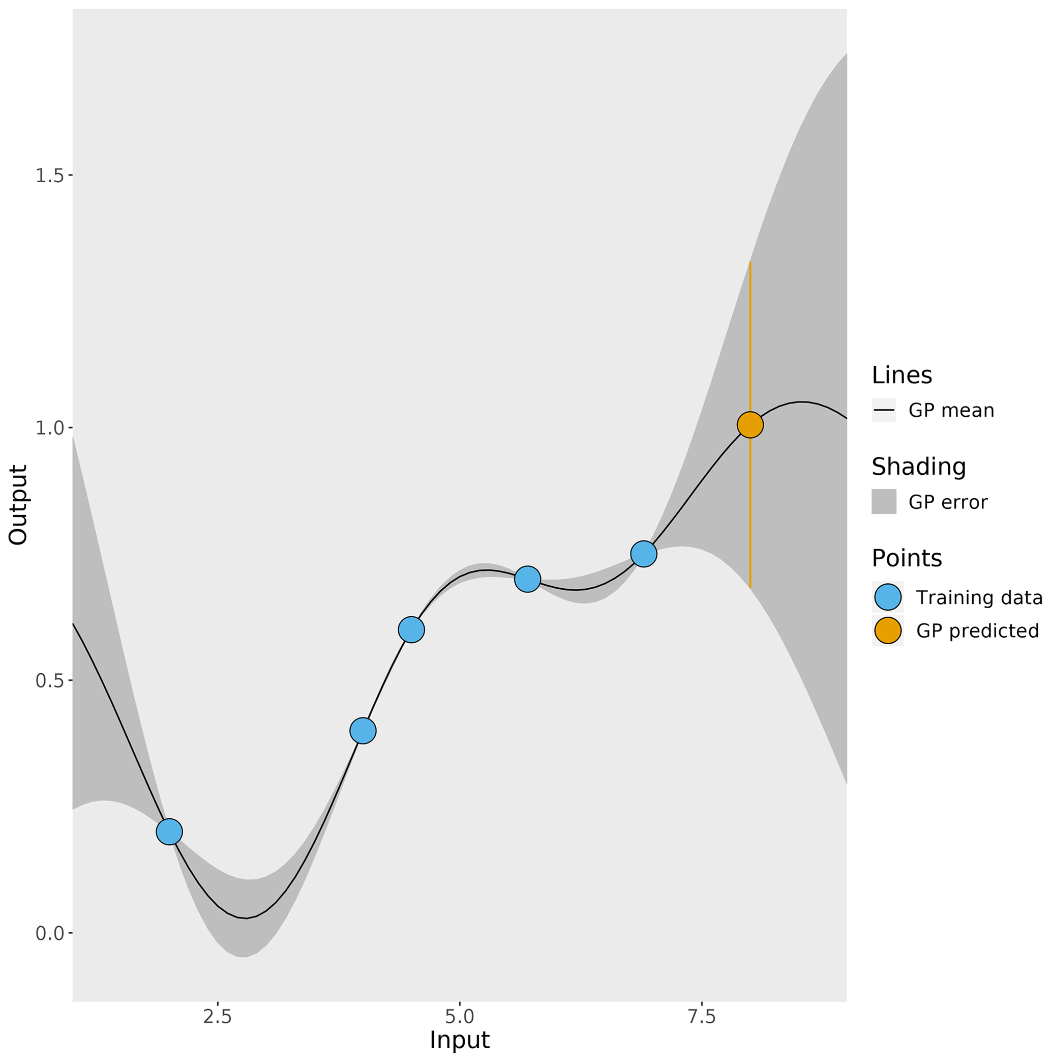
Figure 2A simple 1D example of a Gaussian process (GP). The blue points represent known outputs of the simulator, and the black line is the mean of the Gaussian process which interpolates between the known outputs. The Gaussian-process-estimated uncertainty in its prediction is represented by the grey shading. The orange point is the Gaussian process prediction of an unknown simulator output and the orange bar represent the uncertainty in the prediction.
2.2 The chemical transport model set-up and input parameter ranges
2.2.1 The chemical transport model set-up
This section describes how the 3D CTM, which the emulators will approximate, is set up. The model used is the well-established Model for Ozone and Related Chemical Tracers (MOZART) (Emmons et al., 2010), an offline global 3D CTM. The MOZART model, run in a similar configuration, has been used previously in global methane studies and has been compared to other models and observations (e.g. Patra et al., 2011). In this work, 56 vertical model levels were used, spanning from the Earth's surface up to about 48 km. The model was run with a spatial resolution of 12.00∘ N × 11.25∘ W and a time step of 1 h, with data output on a 6-hourly basis using MERRA reanalysis meteorological fields (Rienecker et al., 2011) from 1995 to 2012.
The MOZART input parameters that are explored in this work describe the methane sources and losses in a similar way to Ganesan et al. (2018). The sources we use as inputs to MOZART are wetlands (Bloom et al., 2017), fresh water (see Supplement), agriculture (Crippa et al., 2018), rice (Yan et al., 2009), waste (Crippa et al., 2018), fossil fuels (Crippa et al., 2018), biomass burning (van der Werf et al., 2010), volcanoes (Etiope and Milkov, 2004), termites (Fung et al., 1991), hydrates (Fung et al., 1991), and oceans (Lambert and Schmidt, 1993; Houweling et al., 1999). The loss processes included in the model are the reactions of methane with the hydroxyl radical (OH) (offline, using fields generated by Spivakovsky et al., 2000), tropospheric chlorine radicals (Cl) (Sherwen et al., 2016), net stratospheric loss (due to reaction with Cl and O(1D)) (Velders, 1995; Patra et al., 2011), and methanotrophic loss in soils (Murguia-Flores et al., 2018). The model input fields are summarised in Table 1. The model input fields are 2D for sources and the soil sink and 3D for the remaining sinks.
The δ13C–CH4 observations are modelled by simulating both 12CH4 and 13CH4. The emissions of these two species are determined by the literature source signatures (Sect. 2.2.2), and the loss differs between the isotopologues according to the literature kinetic isotope effect (Sect. 2.2.2).
For each model simulation, MOZART was spun up using 30 years of repeating meteorology and sources and sinks (nominally representative of the year 1995), starting from a steady-state atmosphere. The model is then run for 1996–2012 with time-varying meteorology, emissions, and losses. To account for any transient signals during the first few years following spin-up (further discussed in Sect. 3.5), only 2000–2012 was analysed. In each simulation, the fields in Table 1 provide the spatial and temporal distribution of the emissions and losses. The total global magnitude of the fields are scaled by the range of values discussed in Sect. 2.2.2 in order to investigate the sensitivity of the methane observations.
(Bloom et al., 2017)Stell, 2020a(Crippa et al., 2018)Yan et al. (2009)(Crippa et al., 2018)(Crippa et al., 2018)(van der Werf et al., 2010)Etiope and Milkov (2004)Fung et al. (1991)Fung et al. (1991)Lambert and Schmidt (1993)Houweling et al. (1999)Spivakovsky et al. (2000)Velders (1995); Patra et al. (2011)Sherwen et al. (2016)Murguia-Flores et al. (2018)Table 1The emission and loss field input to MOZART, their literature sources, their temporal resolution, and the years covered by the fields.
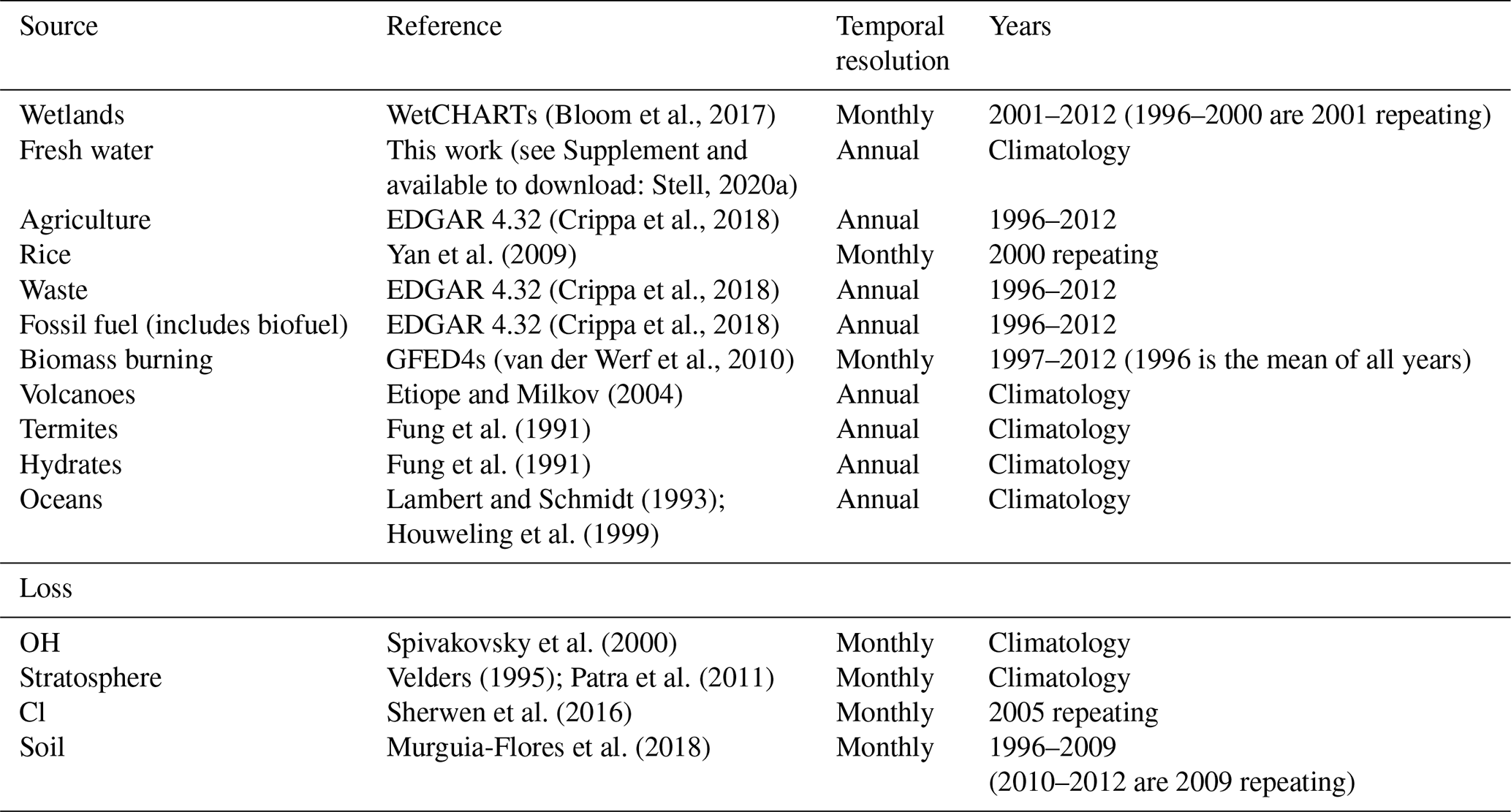
Rice is considered separately to agriculture and wetlands. Biofuel is included in fossil fuel rather than biomass burning. Agricultural burning is included in biomass burning rather than agriculture. The mean of the WetCHARTs ensemble is used for wetland emissions.
2.2.2 The chemical transport model input ranges
We test the sensitivity to five properties of input source and sink parameters: their source magnitudes, source δ13C–CH4 signatures, loss magnitudes, temporal trend variation for the largest emissions or losses, and initial conditions. Several minor terms in the methane budget (termites, hydrates, oceans, and loss kinetic isotope effects) were held constant, and so are not included as inputs to the emulators, in order to simplify the analysis. The uncertainty that results from these minor terms being held constant is explored in Sect. 2.5. The range of possible values for the chosen parameters must be identified so that a set of MOZART simulations over these ranges can be created, which forms the training dataset for the emulators.
The ranges of possible source magnitudes were based on the ranges of compiled literature values in Saunois et al. (2016). The minimum and maximum values from Saunois et al. (2016) have been decreased and increased, respectively, by 10 % in this work as Saunois et al. (2016) do not include the uncertainties in the compiled studies or outliers in their ranges. The ranges of possible δ13C–CH4 source signatures were the 3-standard-deviation ranges in Schwietzke et al. (2016). The ranges of source parameter values used in this work are given in Table 2.
The ranges of possible loss magnitudes were based on Saunois et al. (2016) in the same way as the sources. These ranges do not include some more recent literature values; for example, Wang et al. (2019) suggest a much smaller loss of methane by reaction with Cl. The kinetic isotope effects were held constant at typical literature values (King et al., 1989; Tyler et al., 1994; Saueressig et al., 1995; Reeburgh et al., 1997; Crowley et al., 1999; Snover and Quay, 2000; Tyler et al., 2000; Saueressig et al., 2001) derived as outlined in the Supplement. The reaction rates of methane with OH, Cl, and O(1D) were held constant at the values in Burkholder et al. (2015). While there is some uncertainty in these rate constants, the sensitivity to this term will be similar to that of their respective loss magnitudes. The ranges of loss parameter values used in this work are given in Table 2.
The default temporal trends of the emissions and losses from 1996 to 2012 are set by the input fields in Table 1. The overall inventory or process model trend for the five largest methane emissions or losses (OH, wetlands, fresh water, agriculture, and fossil fuels) was allowed to vary by a linear trend of ± 20 % (± 1.2 % yr−1). For example, a trend parameter that reduces a term by 20 % is applied as a 10 % increase in the first year, decreasing to no change in the middle of the time series, and then decreasing to −10 % in the final year.
Three parameters were varied during the spin-up: the total source magnitude, the total source δ13C–CH4 signature, and an overall imbalance between the source and sink. Table 2 gives the range of these spin-up parameters. The range of the spin-up total source magnitude was derived by considering the minimum and maximum of the sum of the sources in Table 2. The range of the total source δ13C–CH4 signature is constrained to values where the resulting January 1996 initial-condition field has a global surface δ13C–CH4 approximately matching observations (−47.3 ± 0.6 ‰). Similarly, the range of the imbalance between the source and sink is constrained to values where the resulting January 1996 initial-condition field has a global surface methane mole fraction approximately matching observations (1760 ± 30 ppb). However, the January 1996 initial condition can go beyond these observed ranges by varying the other two spin-up parameters. The range of initial-condition values is larger than that considered in previous methane-modelling studies, and it therefore may be an overestimate. However, given that constraints are only typically provided based on surface observations, whereas the initial model fields are 3D, extending from the surface to the upper stratosphere, it is very difficult to determine how uncertain the initial conditions truly are.
Table 2A table of the ranges of the 28 input parameters to MOZART that were varied in the training simulations, hence also in the emulators, and in the sensitivity analysis. Where one value is given, the value is held constant for all training simulations. Where two values are given, they are the lower and upper limit, respectively.
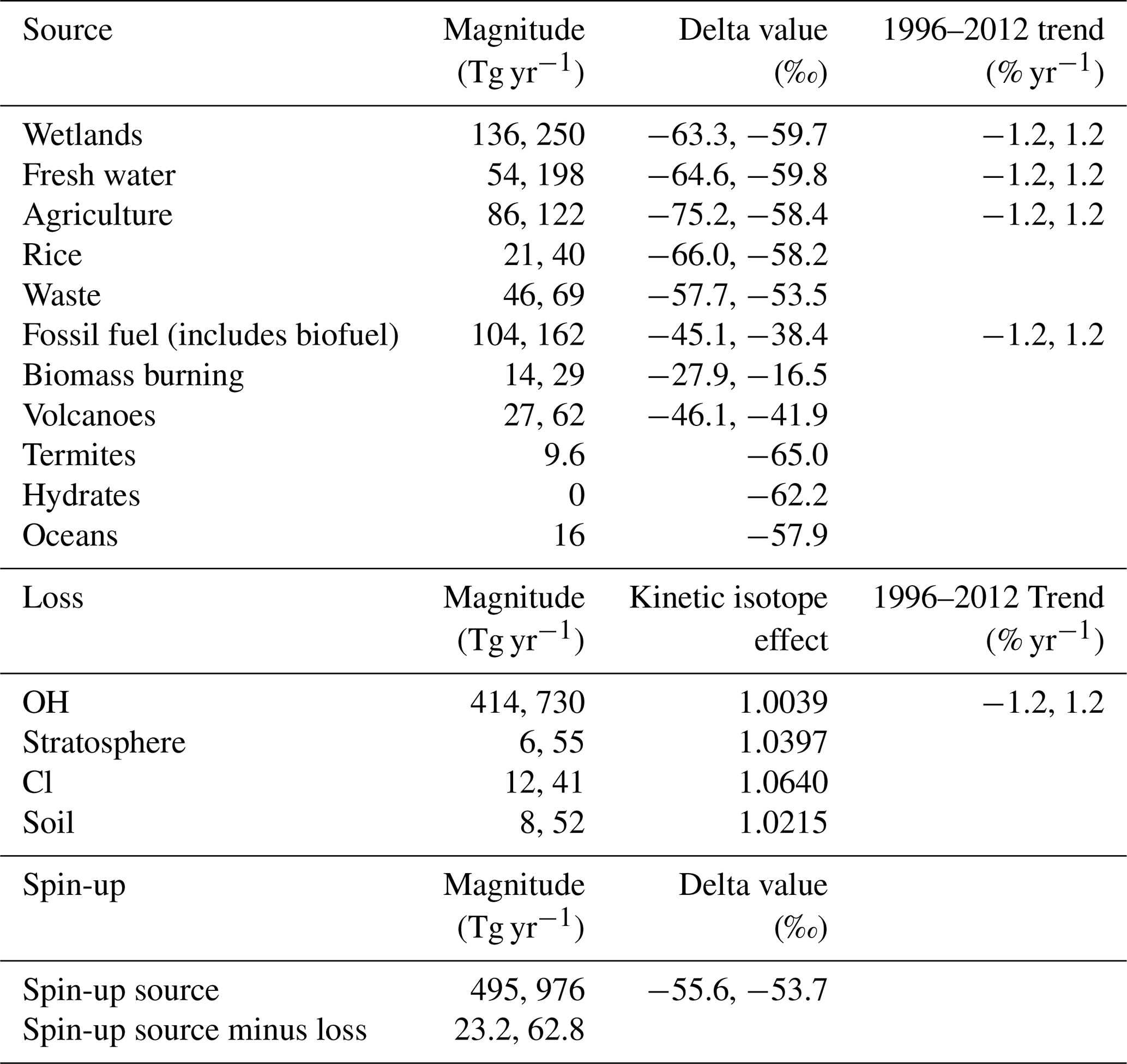
The trend magnitudes are based on a percentage of the original field read into the model, so they could equally be expressed as ± 2.0 Tg yr−1 for wetlands, ± 1.5 Tg yr−1 for fresh water, ± 1.3 Tg yr−1 for agriculture, ± 1.3 Tg yr−1 for fossil fuels, and ± 6.2 Tg yr−1 for OH.
2.3 Creating the chemical transport model training and validation datasets
This section discusses the generation of the training and validation datasets, which is the most computationally expensive part of the analysis as repeated runs of the 3D CTM are required. The training and validation datasets were designed to give accurate emulators for the whole range of the parameter values in Table 2. Therefore, the sets of input parameters in the datasets should be evenly spaced so that every possible input parameter set is close to training data. Hence, each parameter described in Table 2 is assigned a uniform probability distribution over the range given. In order to sample from the distributions in a way that effectively covers the input parameter space, a maximin Latin hypercube was used (McKay et al., 1979; Morris and Mitchell, 1995). A training dataset of 270 MOZART simulations was created and used to build the Gaussian process emulators. We chose 270 simulations as it was found to provide a balance between the accuracy of the emulator and the computational expense of generating training simulations. This is further discussed in the Supplement. An independent maximin Latin hypercube design of 90 MOZART simulations was created as a validation dataset, which was used to evaluate the emulators.
Although observations were not required for this study, for consistency with observed trends, we opted to calculate hemispheric averages based on mole fractions and δ13C–CH4 at grid cells where baseline observations were made by the Global Monitoring Laboratory (GML) Carbon Cycle group, part of the US National Oceanic and Atmospheric Administration (NOAA) (Dlugokencky et al., 1994, 2017), and the Institute of Arctic and Alpine Research (INSTAAR) (Miller et al., 2002; White et al., 2018), respectively. Measurement stations that do not have approximately continuous records for the period of interest (more than 9 out of 13 years) were discarded. We also discarded measurement sites that exhibited substantial above-baseline variability in the model (likely an artefact of the coarse model resolution).
The MOZART outputs are monthly time series describing the Southern Hemisphere mole fraction, the Northern Hemisphere mole fraction, the Southern Hemisphere δ13C–CH4, and the Northern Hemisphere δ13C–CH4. These four 3D CTM outputs are the quantities that the Gaussian processes emulate. However, it should be trivial to extend this to individual grid cells of the 3D CTM in future work. This number of emulators is feasible as the same training dataset could be used, and the computational burden of both building and running the emulator is far smaller than creating the 3D CTM training simulations.
In order to explore sensitivities to quantities that are more often used (either implicitly or explicitly) to inform the global methane budget, the hemispheric outputs are combined as a global mean, inter-hemispheric difference, and trend of the mole fraction and δ13C–CH4. The global mean is defined as the temporal mean of the mean over the northern and southern hemispheres for all months between 2000 and 2012. The inter-hemispheric difference is the temporal mean over the Northern Hemisphere minus the Southern Hemisphere, averaged over all months between 2000 and 2012. The trend is defined as the global mean in December 2012 minus December 2000.
2.4 Gaussian process emulators
2.4.1 The basics of Gaussian process emulation
The Gaussian process is defined by two functions that vary depending on the input parameter values: the mean function and the covariance function. It is sufficient to have a mean function of 0, though in this work, a multiple linear regression was chosen as the system is close to linear. A linear mean function does not stop the Gaussian process from being able to model non-linear relationships. The covariance function is a measure of the similarity of input sets, and as the distance between the inputs increase, the value of the function decreases. In this work we use the squared exponential covariance function as there are no discontinuities or sharp changes in the methane observations due to input parameter variation. The (i,j)th element of the covariance matrix (K) is given by
where the maximum covariance is , xk is the value of the kth input parameter, and lk is the length-scale parameter to be optimised during training.
In this work, the input parameters are the 28 scaling factors in Table 2, and the outputs are the MOZART hemispheric average mole fraction and δ13C–CH4 values. The prediction of an output value (y∗) at a set of input parameters (x∗) samples from the joint multivariate Gaussian distribution of the training data (y) and the predicted values, which follows
where m is the mean function, and x is the training dataset inputs. This means that the expected value of y∗ is
and the uncertainty, in terms of variance, in the estimate is
The Gaussian process emulation method is further described in Rasmussen and Williams (2006), and some simple tutorials are available in O'Hagan (2006) and Ebden (2015).
2.4.2 Gaussian process emulation for time series outputs
Each MOZART output is a time series of 156 months (12 months for each of 13 years) of hemispheric median mole fraction or δ13C–CH4. These 156 monthly outputs are highly correlated in time, which can be exploited in the design of the emulator covariance matrix to minimise information loss. There will also be correlations in space between the northern- and southern-hemispheric outputs, but these correlations are not considered in this work. The chosen covariance matrix (Σ) is composed of the Kronecker product of a temporal covariance matrix (Σt) and a parameter covariance matrix (Σx),
The elements of Σt and Σx are described by ζij and ηij, respectively. The chosen temporal covariance is a first-order autoregressive model (its value depends only on the previous month), and its (i,j)th element is
where ρ is the autocorrelation parameter, and t is the month. The chosen parameter covariance is a squared exponential, and its (i,j)th element is given by Eq. (2).
The emulator parameters (ρ in Eq. 7, σf and lk in Eq. 2) are optimised by maximising the log-likelihood function
This log-likelihood function is maximised using a bounds-constrained quasi-Newton method (Gay, 1990) started from 28 different random points, and the emulator with the maximum log-likelihood is chosen. This set-up uses an adaptation of the R package Stilt (Olson et al., 2018).
2.5 Validation of the emulators
It is important to check that the emulators are an accurate approximation of the 3D CTM before they are used. The validation dataset is used to confirm this because it contains inputs and known 3D CTM outputs that the emulator was not trained on. The emulator predictions for the validation dataset inputs can be compared to the 3D CTM output, and these differences reveal how accurate the approximation is. There are several graphical comparison methods presented in the Supplement, but the main focus is the absolute error in emulation. For the emulators to be useful, their error in emulating the CTM output must be much smaller than a reasonable estimate of the other errors in the system.
The error in a complex model is difficult to calculate, and so it is often ignored; expert judgement is used; or estimates of model–data mismatch uncertainties are approximated, e.g. based on spatial or temporal variability in the model output in the vicinity of observation points (e.g. Chen and Prinn, 2006). In this work, the uncertainty in the 3D CTM is approximated by the uncertainty due to the invariant parameters (as in Vernon et al., 2010). The invariant parameters and their investigated ranges are given in Table 3. The uncertainty was calculated with a maximin Latin hypercube design of 90 MOZART simulations, where variations were allowed only in those parameters held constant in the emulator training dataset. This invariant parameter error does not include many other sources of error (e.g. model transport uncertainties are not addressed) and higher-order “invariant parameter errors” (e.g. erroneous trends or spatial distributions), so it can be considered a lower bound of the total 3D CTM error.
Table 3The ranges of the invariant parameters explored (from the literature as in Sect. 2.2.2), where the first number is the minimum, and the second number is the maximum. The 13CH4 A factor is the Arrhenius pre-exponential factor, which is changed in the model to describe uncertainty in the kinetic isotope effect with respect to the losses. The OH and 13CH4 A factor was also considered, but MOZART only allows the rate constant to be input with two decimal places, and the OH and 13CH4 A factor is constant when given to two decimal places over the range of kinetic isotope effects explored.
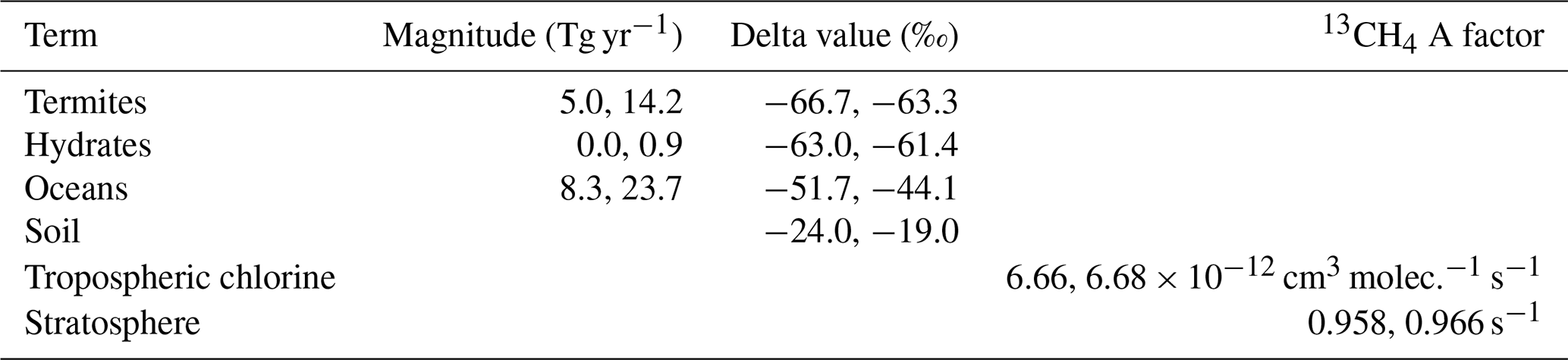
Methane loss by soil was input to the model as negative emissions; hence its isotopic fractionation is not characterised by an A factor.
2.6 Calculation of sensitivity indices
The sensitivity analysis, using the validated emulators, identifies how sensitive the 3D CTM outputs are to changes in the inputs. A variance-based sensitivity analysis requires ∼106 simulations, which would be unfeasible using the 3D CTM as the model is so computationally expensive. By using an emulator, the only 3D CTM simulations required are those needed to train the emulators.
In a variance-based sensitivity analysis, the model sensitivity is quantified using sensitivity indices. These indices measure the proportion of the output variance caused by an input parameter being varied over its possible range (Saltelli et al., 2000). In this work, two sensitivity indices are calculated: the first-order and total effect indices. The first-order sensitivity index reflects the proportion of the variance in the output that can be attributed to a single parameter. This can be calculated as
where V[E(y∣xk)] is the variance in the expected value of the emulator output y given the value of parameter xk, and V(y) is the variance in the emulator output caused by all parameters.
The total effect index is the proportion of the output variance that can be explained by a single parameter and its interactions with other parameters. This can be calculated as
where is the variance in y caused by all parameters except xk. A parameter’s interactions with all other parameters can be calculated by subtracting the first-order sensitivity index from the total sensitivity index. These sensitivity indices were calculated using Monte Carlo methods (Saltelli et al., 2000), and further details are given in the Supplement.
Here, we demonstrate the accuracy of the emulators and show how they can be applied to a sensitivity study of the global methane budget. Section 3.1 compares the 3D chemical transport model (CTM) training dataset to the observations in order to check that the observations lie within the envelope of the model output ensemble. Section 3.2 examines the size of the 3D CTM invariant parameter error, which is compared to the emulator error in Sect. 3.3 in order to justify the use of emulation. The Gaussian process emulation method is then shown to be warranted by comparison to a simpler multiple linear regression in Sect. 3.4. Having demonstrated the utility of the method, a sensitivity analysis is presented in Sect. 3.5.
3.1 Comparison of 3D chemical transport model training dataset to observations
The training dataset is compared to observations to check that the observations lie within the envelope of the MOZART output ensemble. The MOZART simulations used to train the emulators are shown in Fig. 3. The outputs that are considered in the sensitivity analysis (the temporal mean of the global mean, the temporal mean of the inter-hemispheric difference, and the trend in the global mean (Sect. 2.3) for the mole fraction and δ13C–CH4) are presented in Fig. 4. In these figures, the distribution of the MOZART simulations (in orange) is compared to the NOAA and INSTAAR atmospheric observations presented in Rigby et al. (2017) (in black) (derived from a slightly different subset of measurement stations to those used in this work).
These figures demonstrate the large range of methane mole fraction and δ13C–CH4 values covered by the training dataset. This is caused by the large range of emission, loss, and initial-condition values (Sect. 2.2.2). Additionally, the figures show that the observations are within the MOZART range for all outputs.
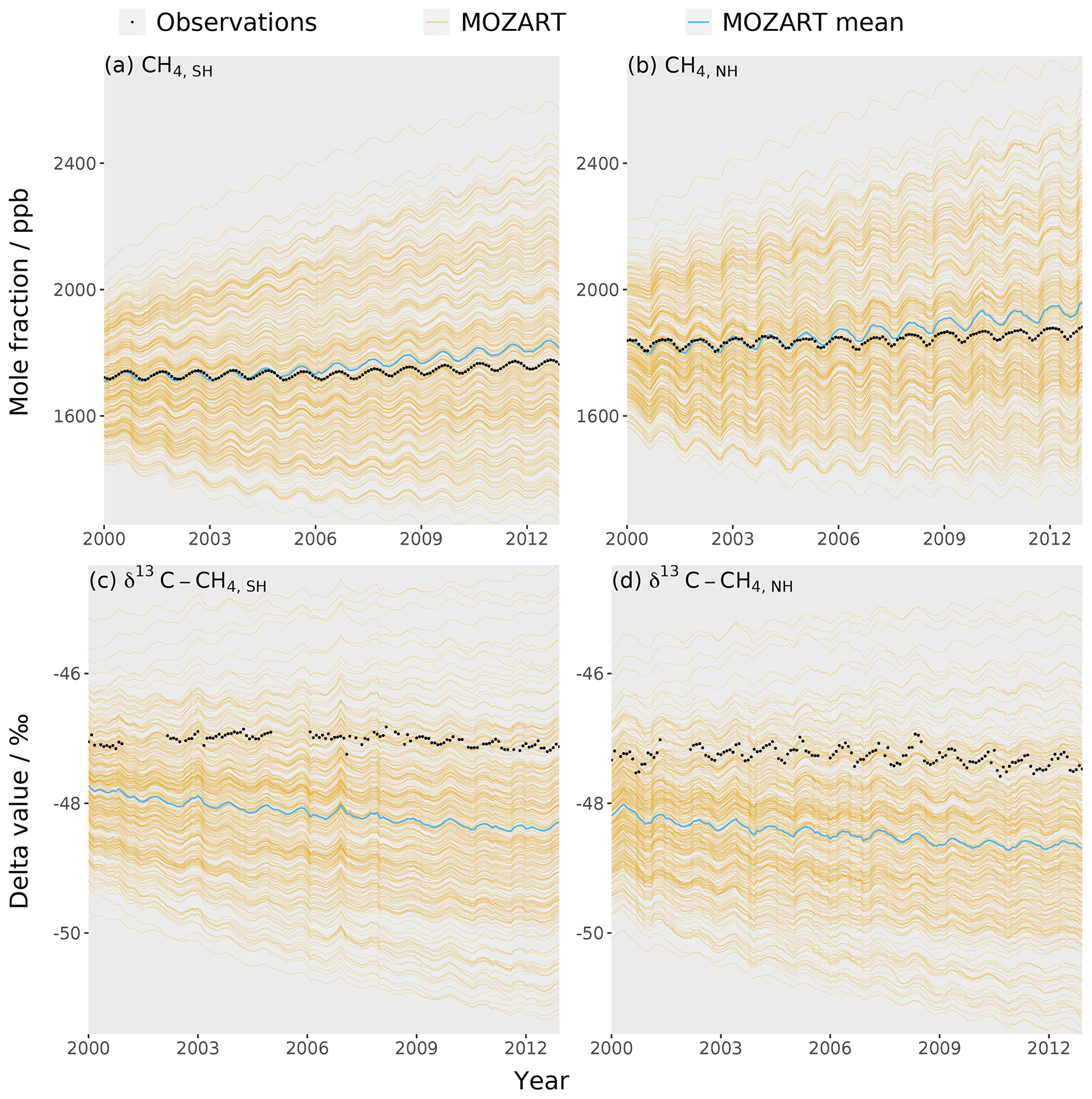
Figure 3The MOZART training dataset (orange lines), the mean MOZART output (blue line), and the observations (black line) for each of the four emulators: (a) the Southern Hemisphere mole fraction, (b) the Northern Hemisphere mole fraction, (c) the Southern Hemisphere δ13C–CH4, and (d) the Northern Hemisphere δ13C–CH4. The observations are hemispheric averages based on NOAA and INSTAAR data (derived from a slightly different subset of measurement stations to those used in this work) presented in Rigby et al. (2017).
These figures also show that the range of MOZART inter-hemispheric-difference values is small compared to the range of global mean and trend values. Ideally, the spatial distributions of the emissions and losses would also be parameterised, allowing greater variation in the inter-hemispheric differences. However, only a limited number of parameters can be included in the Gaussian process emulation method of this work. The more parameters, the more 3D CTM simulations are required to train the emulator and the slower computation becomes. Therefore, only up to about 30 parameters are typically included in a Gaussian process, whereas methods such as adjoint models (e.g. Bousquet et al., 2011; Bergamaschi et al., 2013) can include thousands of parameters.

Figure 4Histograms of the 270 3D CTM training simulations for six outputs: (a) mole fraction global mean, (b) δ13C–CH4 global mean, (c) mole fraction inter-hemispheric difference, (d) δ13C–CH4 inter-hemispheric difference, (e) mole fraction trend, and (f) δ13C–CH4 trend. The black line is the corresponding value for the NOAA and INSTAAR atmospheric observations (Sect. 2.3), which are hemispheric averages (derived from a slightly different subset of measurement stations to those used in this work) presented in Rigby et al. (2017).
3.2 The 3D chemical transport model invariant parameter error
The MOZART invariant parameter error (Sect. 2.5), as far as we are aware, has not been considered in previous methane-modelling studies. This error was calculated as the standard deviation in the output of the set of simulations where parameters not included in the emulator training dataset (fluxes from termites, hydrates, and oceans as well as isotopic fractionation by soil, tropospheric Cl, and stratospheric losses) were perturbed within their uncertainty ranges (Table 3). Over the 13-year period of our study, the mean invariant parameter uncertainty is about 10 ppb and 0.1 ‰ for the mole fraction and δ13C–CH4, respectively. These values are generally slightly larger than the estimate of the combined measurement and model representation uncertainty, which examines the limited temporal and spatial resolution of the model (further details in the Supplement). Additionally, the invariant parameter uncertainty is large compared to atmospheric-methane trends (e.g. between 2000 and 2012, the methane mole fraction and δ13C–CH4 changed by around 40 ppb and −0.1 ‰, respectively). Furthermore, these uncertainties are highly correlated through the study period and therefore effectively act as a substantial bias. The omission of this substantial source of error will likely be leading to an underestimation of uncertainties in emissions and losses derived in inverse-modelling studies or may contribute to the misallocation of some emission or loss to particular processes.
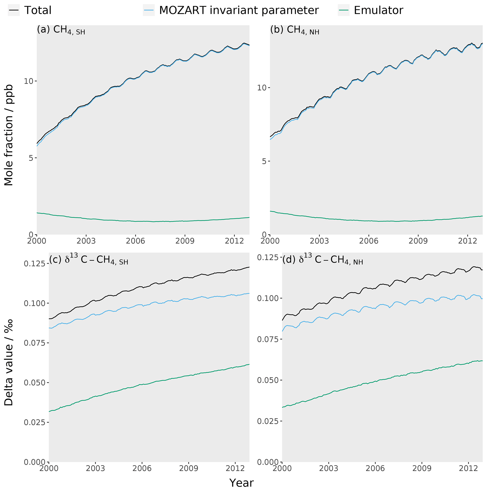
Figure 5The MOZART error (blue line), emulator error (green line), and total error (MOZART and emulator errors added in quadrature) (black line) for each of the four emulators: (a) the Southern Hemisphere mole fraction, (b) the Northern Hemisphere mole fraction, (c) the Southern Hemisphere δ13C–CH4, and (d) the Northern Hemisphere δ13C–CH4.
3.3 Validation of the emulators
Before using the emulators, it is important to check that they reproduce the 3D CTM output well. A more complete analysis can be found in the Supplement, which shows that the emulator is an unbiased representation of the 3D CTM. The emulator error was calculated by predicting the validation dataset (Sect. 2.3) and comparing the predictions to the MOZART output using the root-mean-square error (RMSE),
where yem is the emulator output, ymzt is the MOZART output, and n is the number of simulations being compared. The RMSE was calculated to be about 1.0 ppb and 0.05 ‰ for the mole fraction and δ13C–CH4, respectively. This emulator error is small when compared to the MOZART invariant parameter error (Sect. 2.5) in Fig. 5.
As the MOZART invariant parameter error is significantly larger than the emulator error, it is possible to use a less accurate emulator that requires fewer training simulations. As making the training dataset is the longest step in the process, this would be beneficial for more time-consuming higher-resolution models. In the case of MOZART, we find that only around 90 simulations may be required, which is further discussed in the Supplement.
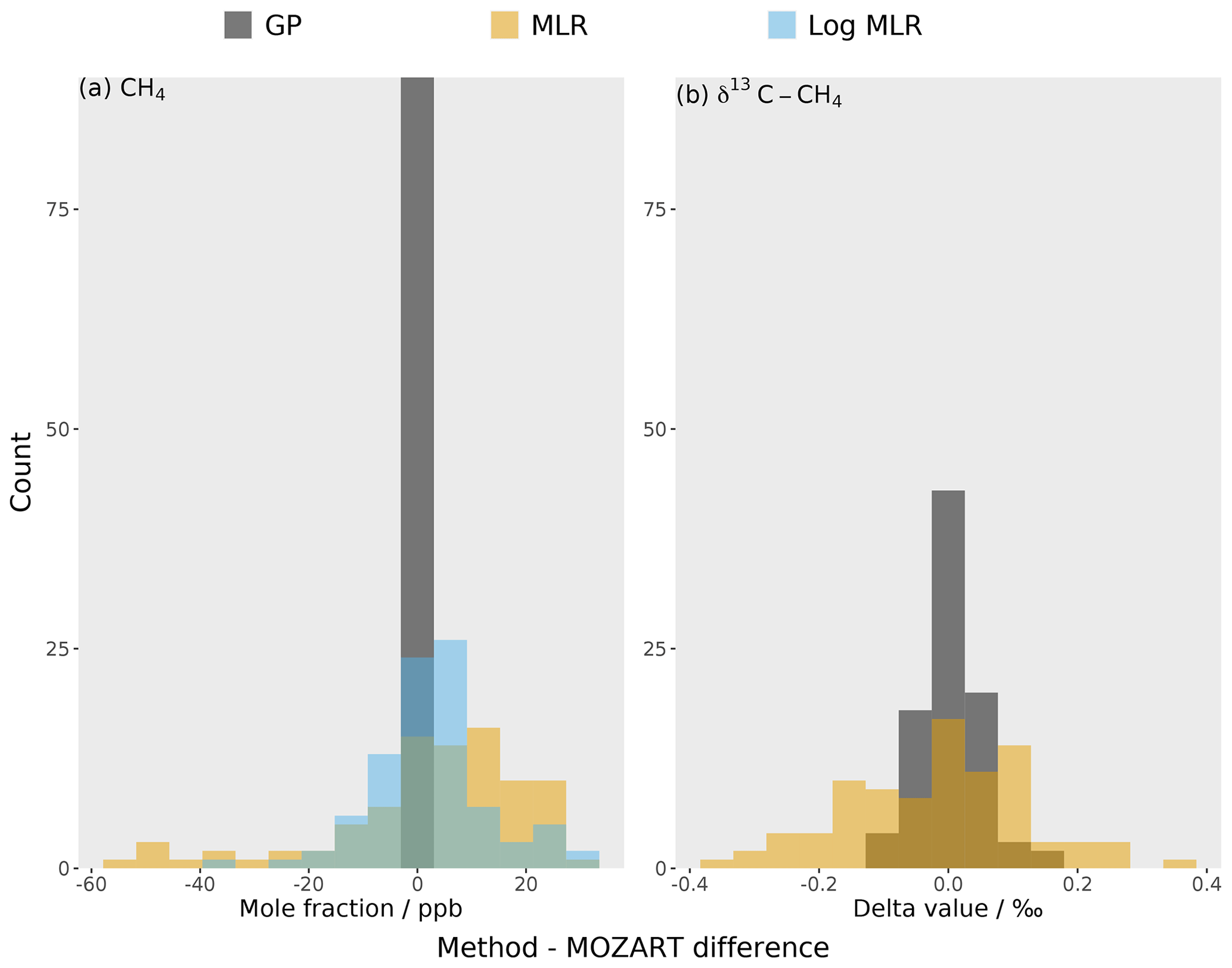
Figure 6The residuals for the global mean between the different emulation methods (in different colours) and the true MOZART output for (a) methane mole fraction and (b) δ13C–CH4. Each emulator is built using a Gaussian process (GP) (grey) or multiple linear regression (MLR) (orange). The mole fraction has an additional emulator: a multiple linear regression with log-transformed OH (blue).
3.4 Comparison of multiple linear regression and the Gaussian process
Previous studies (e.g. McNorton et al., 2018) have assumed that for small changes in the source and loss magnitudes, the relationship between methane sources and losses and atmospheric mole fraction and δ13C–CH4 is linear and that the parameters do not interact (Sect. 3.5). If these two conditions are true or close to true, then multiple linear regression would be able to emulate the 3D CTM. Multiple linear regression might be preferred to a Gaussian process as it requires a smaller training dataset (hence fewer 3D CTM simulations) and is conceptually and computationally simpler. Therefore, this section compares the performance of multiple linear regression and the Gaussian process as emulators of the 3D CTM.
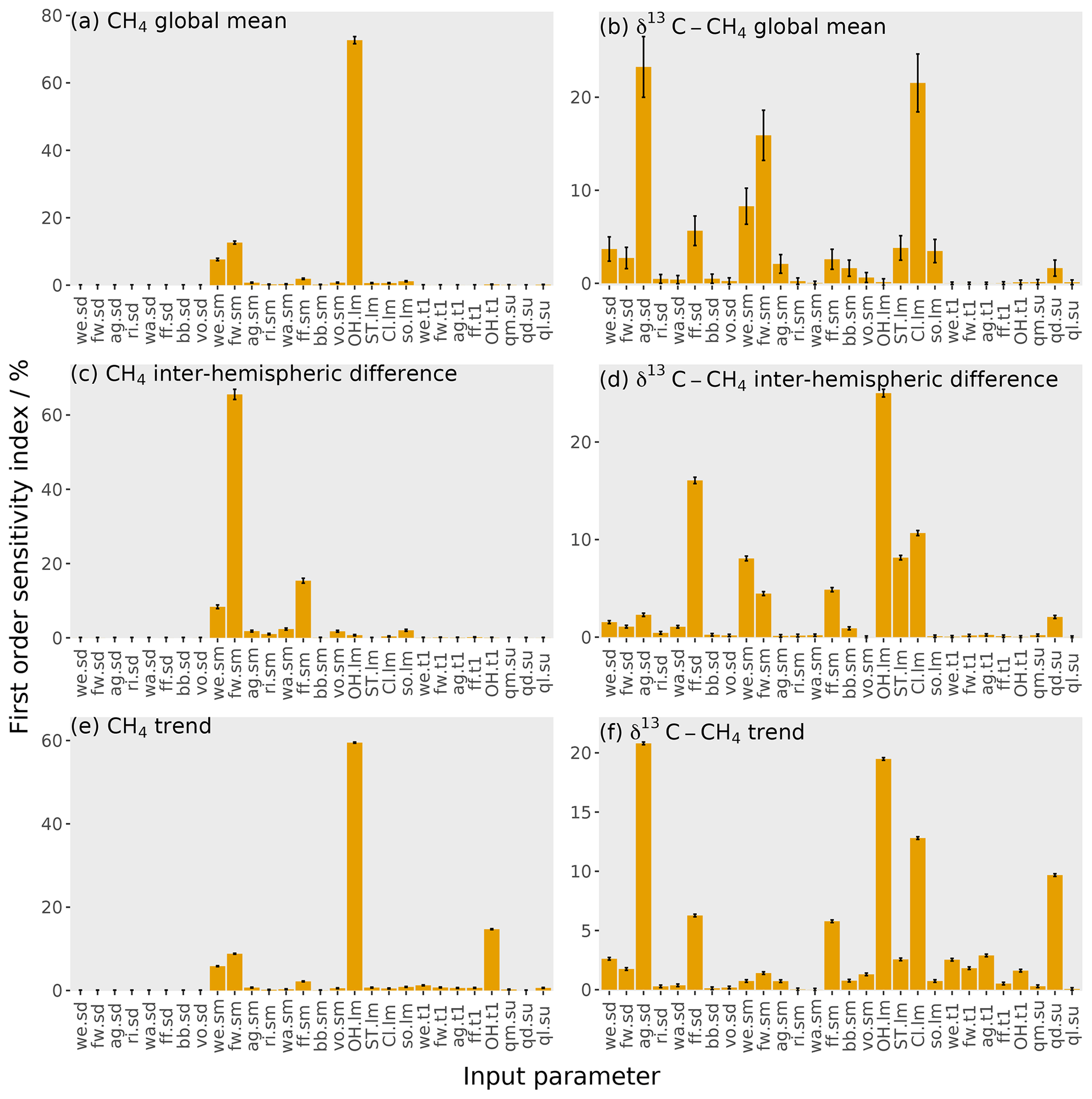
Figure 7The orange bars show the first-order sensitivity coefficients to the input parameters, with the error bars showing the uncertainty in these indices (calculated using bootstrap resampling; see Supplement). Each panel is for one of six outputs: (a) mole fraction global mean, (b) δ13C–CH4 global mean, (c) mole fraction inter-hemispheric difference, (d) δ13C–CH4 inter-hemispheric difference, (e) mole fraction trend, and (f) δ13C–CH4 trend. The values given here are for the temporal mean of the time series. The input parameter codes are given by a combination of a two-character code giving the source or loss (wetlands, we; fresh water, fw; agriculture, ag; rice, ri; waste, wa; fossil fuels, ff; biomass burning, bb; volcanoes, vo; hydroxyl radical, OH; stratospheric, ST; Cl radical, Cl; soil, so; total source magnitude, qm; total source δ13C–CH4 signature, qd; total loss imbalance, ql) and another code giving the type of parameter (source δ13C–CH4 signature, sd; source magnitude, sm; loss magnitude, lm; temporal trend, t1; spin-up, su).
The residuals for the global mean between the 3D CTM validation dataset and the predictions from the two methods (multiple linear regression and the Gaussian process) are compared in Fig. 6. The Gaussian process residuals, with an RMSE of 0.9 ppb and 0.05 ‰, are much smaller than for multiple linear regression, for which they are 19 ppb and 0.14 ‰. In comparison to the MOZART invariant parameter error (10 ppb and 0.1 ‰), the multiple linear regression residuals are large, unlike the Gaussian process (Sect. 3.3). Therefore, the multiple linear regression struggles to emulate MOZART with the required accuracy.
The multiple linear regression accuracy can be improved by considering the non-linearity of the mole fraction with respect to the OH loss. By using a log-transformed OH parameter to estimate the mole fraction, the RMSE becomes 11 ppb (the complete residual distribution is shown in Fig. 6). Multiple linear regression using a log-transformed OH parameter still has a significantly larger RMSE than the Gaussian process, implying that the remaining small non-linearities and parameter interactions are important for predicting the output value. This finding suggests that inverse-modelling studies that have assumed linear and independent sensitivities between observations and source and sink parameters may have underestimated their posterior uncertainties.
3.5 Using the emulators for sensitivity analysis
3.5.1 First-order sensitivity indices
In this section, we examine the sensitivity of the MOZART outputs to the input parameters describing methane sources and sinks. This sensitivity is explored using the first-order sensitivity indices (Eq. 9) in Fig. 7, which show the proportion of the variance of the MOZART output caused by varying each parameter.
The sensitivity of the global mean mole fraction is shown in Fig. 7a and is dominated by the OH loss magnitude (73 %), with considerable contributions from the freshwater (13 %) and wetlands (8 %) source magnitudes. These sensitivities follow the absolute size of the uncertainty in the source and loss magnitudes seen in Fig. 1 and are therefore relatively unsurprising. However, these results highlight the overwhelming importance of global mean OH concentration in determining the global methane mole fraction and the major influence of freshwater emission uncertainties, which have largely been ignored in recent global modelling studies.
Figure 7b shows the sensitivity of the global mean δ13C–CH4 to each input parameter. The parameters that this output is most sensitive to are the agricultural source δ13C–CH4 signature (23 %), the Cl sink magnitude (22 %), and the freshwater source magnitude (16 %), with a couple of other parameters contributing substantially: the wetlands source magnitude (8 %) and the fossil fuels δ13C–CH4 signature (6 %). As the mole fraction and δ13C–CH4 are most sensitive to different parameters, this means that the δ13C–CH4 could be a useful additional measurement for constraining the methane budget. However, two of the parameters that δ13C–CH4 is most sensitive to are δ13C–CH4-specific (the agricultural and fossil fuel source δ13C–CH4 signatures) and so do not, on their own, add information about the magnitudes of the different methane sources and sinks. Unlike the global mean mole fraction, the ordering of the parameters to which δ13C–CH4 is most sensitive does not simply follow the absolute magnitude of uncertainty in the input parameters. The global mean δ13C–CH4 is most sensitive to the agricultural source δ13C–CH4 signature, which has a large uncertainty compared to other source δ13C–CH4 signatures. Additionally, this source δ13C–CH4 signature is substantially more negative than the atmospheric δ13C–CH4 in comparison to other sources, and so this parameter results in a large output variance in the global mean δ13C–CH4. The second-highest contribution to the output variance is the Cl loss magnitude, which has a small uncertainty in comparison to other parameters. However, this loss is highly fractionating, so it has a large impact on the δ13C–CH4. The third-highest contribution is from the freshwater source magnitude as this source has a large uncertainty, and its source δ13C–CH4 signature is substantially more negative than the atmospheric δ13C–CH4. Interestingly, in this investigation, global mean δ13C–CH4 has almost no sensitivity to the magnitude of the OH sink. As we show in the Supplement, this finding is because the transient response of global mean δ13C–CH4 to a change in the OH concentration exhibits a sign change, which coincidentally falls almost exactly at the centre of the period we investigate. Therefore, while the change in OH concentration at the beginning of our simulation causes a significant change in global δ13C–CH4 during the years 2000 and 2012 (with opposite signs), these changes roughly cancel in the 2000–2012 mean.
The mole fraction inter-hemispheric difference (the temporal mean over the Northern Hemisphere minus the Southern Hemisphere as in Sect. 2.3) is most sensitive to the freshwater (66 %), fossil fuel (15 %), and wetlands (8 %) source magnitudes, as shown in Fig. 7c. The sensitivity to these parameters is due to their large uncertainties and large differences in emissions between the two hemispheres. The OH loss magnitude, which has the largest uncertainty in any parameter, has been assumed to be close to equally distributed between the hemispheres (Patra et al., 2014), hence its low sensitivity with respect to this output. However, had the uncertainty in the hemispheric distribution of OH been included in our analysis, it would likely have explained a larger proportion of this sensitivity. The dominant role of freshwater emission uncertainty in determining the inter-hemispheric difference further highlights the need to better understand this part of the methane budget.
Figure 7d shows the sensitivity of the δ13C–CH4 inter-hemispheric difference. The parameters that the δ13C–CH4 inter-hemispheric difference is most sensitive to are the OH loss magnitude (25 %), the fossil fuel source δ13C–CH4 signature (16 %), and the Cl sink magnitude (11 %). There are also significant contributions from the wetlands source magnitude (8 %) and the stratospheric loss magnitude (8 %). The parameters to which the δ13C–CH4 inter-hemispheric difference is most sensitive are similar to those that most strongly influence the global mean δ13C–CH4 but with a higher sensitivity to parameters with a large inter-hemispheric difference (e.g. fossil fuels). The exception is the sensitivity to the OH loss magnitude, which strongly impacts the inter-hemispheric difference but not the global mean (which is somewhat coincidental, as discussed above and in the Supplement).
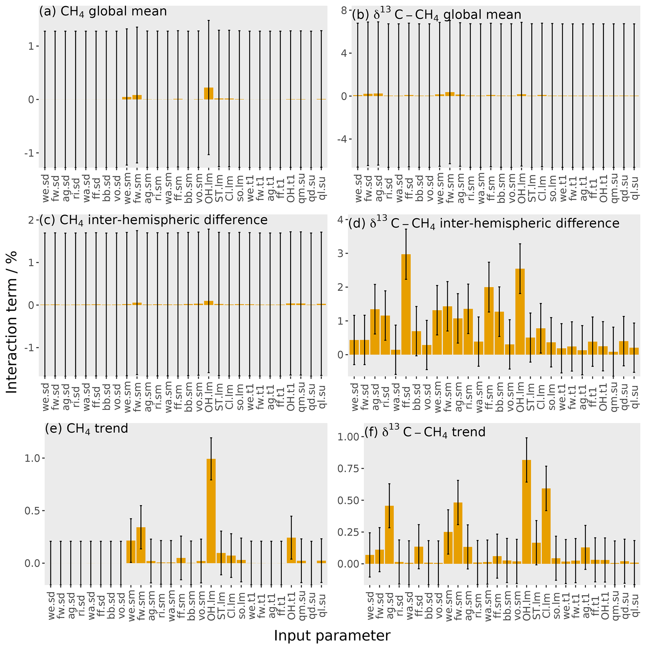
Figure 8The orange bars show the interaction terms of the parameters, with the error bars showing the uncertainty in these interactions (calculated using bootstrap resampling; see Supplement). Each panel shows one output: (a) mole fraction global mean, (b) δ13C–CH4 global mean, (c) mole fraction inter-hemispheric difference, (d) δ13C–CH4 inter-hemispheric difference, (e) mole fraction trend, and (f) δ13C–CH4 trend. The values given here are for the temporal mean of the time series. The input parameter codes are given by a combination of a two-character code giving the source or loss (wetlands, we; fresh water, fw; agriculture, ag; rice, ri; waste, wa; fossil fuels, ff; biomass burning, bb; volcanoes, vo; hydroxyl radical, OH; stratospheric, ST; Cl radical, Cl; soil, so; total source magnitude, qm; total source δ13C–CH4 signature, qd; total loss imbalance, ql) and another code giving the type of parameter (source δ13C–CH4 signature, sd; source magnitude, sm; loss magnitude, lm; temporal trend, t1; spin-up, su).
The sensitivity of the mole fraction trend (the global mean in December 2012 minus December 2000 as in Sect. 2.3) is shown in Fig. 7e. The sensitivity is dominated by a single parameter: 59 % of the variance is caused by the uncertainty in the OH loss magnitude. The OH loss trend (15 %), freshwater source magnitude (9 %), and wetlands source magnitude (6 %) also contribute significantly. The OH loss parameter's importance for the output mole fraction value stems from the large uncertainty in the OH loss.
The δ13C–CH4 trend sensitivity is shown in Fig. 7f. The trend is most sensitive to the agricultural source δ13C–CH4 signature (21 %), the OH loss magnitude (19 %), the Cl loss magnitude (13 %), and the spin-up source δ13C–CH4 signature (10 %). There are additional contributions from the fossil fuel source δ13C–CH4 signature (6 %) and the fossil fuel source magnitude (6 %). Parameters that can change the atmospheric global mean δ13C–CH4 will also affect the trend (e.g. the agricultural source δ13C–CH4 and the Cl loss magnitude). Additionally, the trend is sensitive to the OH loss magnitude, despite the global mean being insensitive to this parameter. This sensitivity to OH is explained by the slow (and somewhat counter-intuitive) way that changes in the δ13C–CH4 propagate through the atmosphere and will be dependent on the time period investigated, which is explained in detail in the Supplement. The δ13C–CH4 trend is also sensitive to the spin-up because of the slow response time in the atmospheric δ13C–CH4, meaning that the trend is strongly dependent on its initial value (Tans, 1997). A wide range of spin-up source δ13C–CH4 signature values (Table 2) are examined in this work; however the importance of the spin-up applies to even small ranges. For example, if the spin-up source δ13C–CH4 signature is perturbed by 0.1 ‰ from the initial median parameter values, the output atmospheric-δ13C–CH4 trend changes by 0.04 ‰, almost half the observed δ13C–CH4 trend during this period. Therefore, constraining the initial conditions throughout the atmosphere is a serious challenge if δ13C–CH4 observations are to be used to estimate the recent changes in the methane budget.
These first-order sensitivity indices demonstrate several key challenges in methane inverse-modelling studies. Three parameters that the mole fraction and δ13C–CH4 are highly sensitive to are often not explored in methane modelling: the OH loss is often assumed to be known (e.g. Schaefer et al., 2016; Worden et al., 2017), as is the Cl loss (e.g. Nisbet et al., 2016; Rigby et al., 2017), or the Cl loss is omitted (e.g. Turner et al., 2017). Furthermore, freshwater emissions have not been included as an independent source in global methane studies as far as we are aware. Freshwater bodies emit methane by bacteria breaking down organic matter in an anaerobic environment, as in wetlands, and the freshwater emissions are potentially of similar magnitude to wetlands but more uncertain (as seen in Fig. 1). There has been increasing acknowledgement that OH and Cl could play important roles in methane modelling (e.g. Rigby et al., 2017; Turner et al., 2017; Thanwerdas et al., 2019; Strode et al., 2020), but the role of freshwater methane emissions has not received the same level of attention. This lack of attention is presumably the result of the freshwater source's large uncertainty, but it is this large uncertainty that makes this source so important in constraining the methane budget. The first-order sensitivity indices also demonstrate that the atmospheric δ13C–CH4 is sensitive to some parameters to which the mole fraction is relatively insensitive, so it should provide additional complementary information. However, δ13C–CH4 is also highly sensitive to the initial conditions and some source signatures (e.g. agriculture), which need to be accounted for to realise the value for global-scale studies using these isotopic measurements. Furthermore, these sources of uncertainty need to be carefully considered in methane-modelling studies that use δ13C–CH4 because erroneous assumptions of well-known initial conditions, source δ13C–CH4 signatures, or kinetic isotope effects could have substantial impacts on top-down budget estimates.
3.5.2 Parameter interactions
The interaction between parameters is calculated by subtracting the first-order sensitivity (Eq. 9) from the total effect of each parameter (Eq. 10). The interaction of one particular parameter with all other parameters is the proportion of the output variance explained by changing that parameter alongside all other parameters, removing the proportion of the output variance from changing that parameter independently of all other parameters. An example of interacting parameters is the OH loss and any source for the global mean mole fraction: a lower OH concentration causes a greater mole fraction increase from an increase in emissions.
The parameter interactions are shown in Fig. 8. These interactions are generally small, with the largest being 3 %. The interactions across all parameters account for 12 % of the output variance in the δ13C–CH4 inter-hemispheric difference and at most 2 % for the other five outputs. This means that we can essentially consider the effect of each parameter independently in this sensitivity analysis. For this complex simulator, one-at-a-time sensitivity tests would produce a similar result, though this will not necessarily be the case for other models (Saltelli and Annoni, 2010).
Whilst these interactions are relatively unimportant in this sensitivity analysis, they must be considered in order to build an accurate emulator. For example, the 0.2 % and 0.7 % of the output variance explained by parameter interactions for the global mean mole fraction and δ13C–CH4, respectively, are equivalent to a standard deviation of 10 ppb and 0.09 ‰ in the output. This accounts for most of the difference in performance of the Gaussian process and multiple linear regression, which does not consider parameter interactions, in Sect. 3.4.
We have shown that Gaussian processes allow emulation of a global 3D chemical transport model (CTM) of atmospheric methane, producing a fast and accurate approximation of the response of methane mole fraction and δ13C–CH4 to changes in model input parameters. In this work, 28 parameters were investigated, related to methane sources and sinks, based on 270 forward model simulations. However, we found that, compared to an estimate of model uncertainty, an accurate emulator could be built for this system using fewer than 100 training runs. Our model uncertainty estimate, which we term “invariant parameter error”, was based on an ensemble of model runs in which several minor sources and sinks were perturbed within their estimated uncertainty ranges, showing that they could, when considered together, lead to a substantial, and often ignored, source of uncertainty in global methane-modelling studies (with mean uncertainties in hemispheric-methane mole fraction and δ13C–CH4 between 2000 and 2012 of approximately 10 ppb and 0.1 ‰, respectively).
We show that a Gaussian process outperforms multiple linear regression in emulating the 3D CTM methane simulations: the Gaussian process RMSE is small (0.9 ppb, 0.05 ‰) compared to the invariant parameter error, whereas the multiple linear regression error (19 ppb, 0.14 ‰) is larger. Therefore, the use of Gaussian process emulators does not much reduce how precisely the model matches observations, but multiple linear regression could. The poor performance of the multiple linear regression is primarily because of the parameter interactions and the non-linearity in the response of the mole fraction to the OH loss.
The speed of emulation allows many more 3D CTM outputs to be generated than would be possible running the CTM itself, allowing a wider range of possible analyses. In this work, a thorough sensitivity analysis was carried out, which required millions of runs of the emulator. The sensitivity analysis demonstrated some issues that are critical to consider for global methane modelling. The OH loss, Cl loss, and freshwater source are frequently held constant or not included in methane-modelling studies, but the mole fraction or δ13C–CH4 outputs are highly sensitive to these parameters. Our analysis shows that δ13C–CH4 measurements provide somewhat independent constraints on the sources and sinks of methane as they are sensitive to different model parameters. However, several of these parameters are δ13C–CH4-specific, so they do not, on their own, provide new information on the methane budget but must be well-quantified if δ13C–CH4 observations are to provide budget constraints (e.g. δ13C–CH4 initial conditions or the agricultural source signature).
Whilst we have focused here on a variance-based sensitivity analysis, we anticipate that there could be multiple future applications of an accurate and fast emulator of 3D CTM simulations of atmospheric methane. This system could allow for the calculation of input parameter values that are consistent with observations (history matching) or could allow us to determine the set of parameter values that most probably simulate observations (e.g. through Bayesian inference). While in this work hemispheric emulators were created, it is also possible to emulate individual grid cells in the 3D CTM, which would provide a more accurate representation of the 3D CTM output. This number of emulators is feasible as the same training dataset could be used, and the computational burden of both building and running the emulator is far smaller than creating the 3D CTM training simulations. This allows new and flexible emulators to be built and used for novel applications without the need to rerun the 3D CTM.
The code used to create the freshwater emissions field and the field itself are available at https://doi.org/10.17605/OSF.IO/Q9F8P (last access: 25 August 2020, Stell, 2020a). The code and datasets used to train the emulators and carry out the sensitivity analysis are available at https://doi.org/10.17605/OSF.IO/Z435M (last access: 8 January 2021, Stell, 2020b).
The supplement related to this article is available online at: https://doi.org/10.5194/acp-21-1717-2021-supplement.
ACS, LMW, and MR contributed to the conception and development of the project. TS created the Cl field used in this work. ACS wrote the code and performed the calculations. All authors contributed to the manuscript.
The authors declare that they have no conflict of interest.
We would like to thank the two anonymous reviewers for their suggestions to improve the paper.
This research has been supported by the Natural Environment Research Council (grant nos. NE/N016548/1, NE/M014851/1, and NE/L013088/1).
This paper was edited by Bryan N. Duncan and reviewed by two anonymous referees.
Bergamaschi, P., Brenninkmeijer, C. A. M., Hahn, M., Röckmann, T., Scharffe, D. H., Crutzen, P. J., Elansky, N. F., Belikov, I. B., Trivett, N. B. A., and Worthy, D. E. J.: Isotope analysis based source identification for atmospheric CH4 and CO sampled across Russia using the Trans-Siberian railroad, J. Geophys. Res.-Atmos., 103, 8227–8235, https://doi.org/10.1029/97JD03738, 1998. a
Bergamaschi, P., Houweling, S., Segers, A., Krol, M., Frankenberg, C., Scheepmaker, R. A., Dlugokencky, E., Wofsy, S. C., Kort, E. A., Sweeney, C., Schuck, T., Brenninkmeijer, C., Chen, H., Beck, V., and Gerbig, C.: Atmospheric CH4 in the first decade of the 21st century: Inverse modeling analysis using SCIAMACHY satellite retrievals and NOAA surface measurements, J. Geophys. Res.-Atmos., 118, 7350–7369, https://doi.org/10.1002/jgrd.50480, 2013. a, b, c
Bloom, A. A., Bowman, K. W., Lee, M., Turner, A. J., Schroeder, R., Worden, J. R., Weidner, R., McDonald, K. C., and Jacob, D. J.: A global wetland methane emissions and uncertainty dataset for atmospheric chemical transport models (WetCHARTs version 1.0), Geosci. Model Dev., 10, 2141–2156, https://doi.org/10.5194/gmd-10-2141-2017, 2017. a, b
Bousquet, P., Ringeval, B., Pison, I., Dlugokencky, E. J., Brunke, E.-G., Carouge, C., Chevallier, F., Fortems-Cheiney, A., Frankenberg, C., Hauglustaine, D. A., Krummel, P. B., Langenfelds, R. L., Ramonet, M., Schmidt, M., Steele, L. P., Szopa, S., Yver, C., Viovy, N., and Ciais, P.: Source attribution of the changes in atmospheric methane for 2006–2008, Atmos. Chem. Phys., 11, 3689–3700, https://doi.org/10.5194/acp-11-3689-2011, 2011. a, b, c
Burkholder, J. B., Sander, S. P., Abbatt, J., Barker, J. R., Huie, R. E., Kolb, C. E., Kurylo, M. J., Orkin, V. L., Wilmouth, D. M., and Wine, P. H.: Chemical Kinetics and Photochemical Data for Use in Atmospheric Studies, Evaluation Number 18, Tech. Rep. 10, Jet Propulsion Laboratory, Pasadena, https://doi.org/10.1002/kin.550171010, 2015. a
Chang, W., Applegate, P. J., Haran, M., and Keller, K.: Probabilistic calibration of a Greenland Ice Sheet model using spatially resolved synthetic observations: toward projections of ice mass loss with uncertainties, Geosci. Model Dev., 7, 1933–1943, https://doi.org/10.5194/gmd-7-1933-2014, 2014. a
Chen, Y.-H. and Prinn, R. G.: Estimation of atmospheric methane emissions between 1996 and 2001 using a three-dimensional global chemical transport model, J. Geophys. Res.-Atmos., 111, D10307, https://doi.org/10.1029/2005JD006058, 2006. a, b, c
Coplen, T. B.: Guidelines and recommended terms for expression of stable-isotope-ratio and gas-ratio measurement results, Rapid Commun. Mass Sp., 25, 2538–2560, https://doi.org/10.1002/rcm.5129, 2011. a
Crippa, M., Guizzardi, D., Muntean, M., Schaaf, E., Dentener, F., van Aardenne, J. A., Monni, S., Doering, U., Olivier, J. G. J., Pagliari, V., and Janssens-Maenhout, G.: Gridded emissions of air pollutants for the period 1970–2012 within EDGAR v4.3.2, Earth Syst. Sci. Data, 10, 1987–2013, https://doi.org/10.5194/essd-10-1987-2018, 2018. a, b, c, d, e, f
Crowley, J., Saueressig, G., Bergamaschi, P., Fischer, H., and Harris, G.: Carbon kinetic isotope effect in the reaction CH4+Cl: a relative rate study using FTIR spectroscopy, Chem. Phys. Lett., 303, 268–274, https://doi.org/10.1016/S0009-2614(99)00243-2, 1999. a
Dlugokencky, E., Lang, P., Crotwell, A., Mund, J., Crotwell, M., and Thoning, K.: Atmospheric Methane Dry Air Mole Fractions from the NOAA ESRL Carbon Cycle Cooperative Global Air Sampling Network, 1983-2016, Version: 2017-07-28, available at: ftp://aftp.cmdl.noaa.gov/data/trace_gases/ch4/flask/surface/ (last access: 11 April 2018), 2017. a
Dlugokencky, E. J., Steele, L. P., Lang, P. M., and Masarie, K. A.: The growth rate and distribution of atmospheric methane, J. Geophys. Res., 99, 17021–17043, https://doi.org/10.1029/94jd01245, 1994. a
Ebden, M.: Gaussian Processes: A Quick Introduction, arXiv:1505.02965v2 [math.ST], 2015. a, b
Emmons, L. K., Walters, S., Hess, P. G., Lamarque, J.-F., Pfister, G. G., Fillmore, D., Granier, C., Guenther, A., Kinnison, D., Laepple, T., Orlando, J., Tie, X., Tyndall, G., Wiedinmyer, C., Baughcum, S. L., and Kloster, S.: Description and evaluation of the Model for Ozone and Related chemical Tracers, version 4 (MOZART-4), Geosci. Model Dev., 3, 43–67, https://doi.org/10.5194/gmd-3-43-2010, 2010. a
Etiope, G. and Milkov, A. V.: A new estimate of global methane flux from onshore and shallow submarine mud volcanoes to the atmosphere, Environmental Geology, 46, 997–1002, https://doi.org/10.1007/s00254-004-1085-1, 2004. a, b
Etminan, M., Myhre, G., Highwood, E. J., and Shine, K. P.: Radiative forcing of carbon dioxide, methane, and nitrous oxide: A significant revision of the methane radiative forcing, Geophys. Res. Lett., 43, 12614–12623, https://doi.org/10.1002/2016GL071930, 2016. a
Farah, M., Birrell, P., Conti, S., and Angelis, D. D.: Bayesian Emulation and Calibration of a Dynamic Epidemic Model for A/H1N1 Influenza, J. Am. Stat. Assoc., 109, 1398–1411, https://doi.org/10.1080/01621459.2014.934453, 2014. a
Fung, I., John, J., Lerner, J., Matthews, E., Prather, M., Steele, L. P., and Fraser, P. J.: Three-dimensional model synthesis of the global methane cycle, J. Geophys. Res., 96, 13033–13065, https://doi.org/10.1029/91JD01247, 1991. a, b, c, d, e
Ganesan, A. L., Stell, A. C., Gedney, N., Comyn-Platt, E., Hayman, G., Rigby, M., Poulter, B., and Hornibrook, E.: Spatially Resolved Isotopic Source Signatures of Wetland Methane Emissions, Geophys. Res. Lett., 45, 3737–3745, https://doi.org/10.1002/2018GL077536, 2018. a
Gay, D. M.: Usage Summary for Selected Optimization Routines (PORT Mathematical Subroutine Library, Optimization chapter), Tech. Rep. 153, AT&T Bell Laboratories, Murray Hill, NJ 07974, 1990. a
Hein, R., Crutzen, P. J., and Heimann, M.: An inverse modeling approach to investigate the global atmospheric methane cycle, Global Biogeochem. Cy., 11, 43–76, https://doi.org/10.1029/96GB03043, 1997. a
Houweling, S., Kaminski, T., Dentener, F., Lelieveld, J., and Heimann, M.: Inverse modeling of methane sources and sinks using the adjoint of a global transport model, J. Geophys. Res.-Atmos., 104, 26137–26160, https://doi.org/10.1029/1999JD900428, 1999. a, b, c
Kennedy, M., Anderson, C., O'Hagan, A., Lomas, M., Woodward, I., and Gosling, J. P.: Quantifying uncertainty in the biospheric carbon flux for England and Wales, J. R. Stat. Soc., 171, 109–135, 2008. a
King, S. L., Quay, P. D., and Lansdown, J. M.: The 13C/ 12C kinetic isotope effect for soil oxidation of methane at ambient atmospheric concentrations, J. Geophys. Res., 94, 18273–18277, https://doi.org/10.1029/JD094iD15p18273, 1989. a
Kirschke, S., Bousquet, P., Ciais, P., Saunois, M., Canadell, J. G., Dlugokencky, E. J., Bergamaschi, P., Bergmann, D., Blake, D. R., Bruhwiler, L., Cameron-Smith, P., Castaldi, S., Chevallier, F., Feng, L., Fraser, A., Heimann, M., Hodson, E. L., Houweling, S., Josse, B., Fraser, P. J., Krummel, P. B., Lamarque, J.-F., Langenfelds, R. L., Le Quéré, C., Naik, V., O'Doherty, S., Palmer, P. I., Pison, I., Plummer, D., Poulter, B., Prinn, R. G., Rigby, M., Ringeval, B., Santini, M., Schmidt, M., Shindell, D. T., Simpson, I. J., Spahni, R., Steele, L. P., Strode, S. A., Sudo, K., Szopa, S., van der Werf, G. R., Voulgarakis, A., van Weele, M., Weiss, R. F., Williams, J. E., and Zeng, G.: Three decades of global methane sources and sinks, Nat. Geosci., 6, 813–823, https://doi.org/10.1038/ngeo1955, 2013. a
Lambert, G. and Schmidt, S.: Reevaluation of the oceanic flux of methane: Uncertainties and long term variations, Chemosphere, 26, 579–589, https://doi.org/10.1016/0045-6535(93)90443-9, 1993. a, b
Lee, L. A., Carslaw, K. S., Pringle, K. J., Mann, G. W., and Spracklen, D. V.: Emulation of a complex global aerosol model to quantify sensitivity to uncertain parameters, Atmos. Chem. Phys., 11, 12253–12273, https://doi.org/10.5194/acp-11-12253-2011, 2011. a
Lee, L. A., Carslaw, K. S., Pringle, K. J., and Mann, G. W.: Mapping the uncertainty in global CCN using emulation, Atmos. Chem. Phys., 12, 9739–9751, https://doi.org/10.5194/acp-12-9739-2012, 2012. a
McKay, M. D., Beckman, R. J., and Conover, W. J.: A Comparison of Three Methods for Selecting Values of Input Variables in the Analysis of Output From a Computer Code, Technometrics, 21, 239–245, https://doi.org/10.1080/00401706.2000.10485979, 1979. a
McNorton, J., Wilson, C., Gloor, M., Parker, R. J., Boesch, H., Feng, W., Hossaini, R., and Chipperfield, M. P.: Attribution of recent increases in atmospheric methane through 3-D inverse modelling, Atmos. Chem. Phys., 18, 18149–18168, https://doi.org/10.5194/acp-18-18149-2018, 2018. a, b, c, d
Miller, J. B., Mack, K. A., Dissly, R., White, J. W., Dlugokencky, E. J., and Tans, P. P.: Development of analytical methods and measurements of 13C/12C in atmospheric CH4 from the NOAA Climate Monitoring and Diagnostics Laboratory Global Air Sampling Network, J. Geophys. Res.-Atmos., 107, 4178, https://doi.org/10.1029/2001JD000630, 2002. a
Miller, S. M., Michalak, A. M., Detmers, R. G., Hasekamp, O. P., Bruhwiler, L. M. P., and Schwietzke, S.: China's coal mine methane regulations have not curbed growing emissions, Nat. Commun., 10, 303, https://doi.org/10.1038/s41467-018-07891-7, 2019. a
Morris, M. D. and Mitchell, T. J.: Exploratory designs for computational experiments, J. Stat. Plan. Infer., 43, 381–402, https://doi.org/10.1016/0378-3758(94)00035-T, 1995. a
Murguia-Flores, F., Arndt, S., Ganesan, A. L., Murray-Tortarolo, G., and Hornibrook, E. R. C.: Soil Methanotrophy Model (MeMo v1.0): a process-based model to quantify global uptake of atmospheric methane by soil, Geosci. Model Dev., 11, 2009–2032, https://doi.org/10.5194/gmd-11-2009-2018, 2018. a, b
Myhre, G., Shindell, D., Bréon, F.-M., Collins, W., Fuglestvedt, J., Huang, J., Koch, D., Lamarque, J.-F., Lee, D., Mendoza, B., Nakajima, T., Robock, A., Stephens, G., Takemura, T., and Zhang, H.: Anthropogenic and Natural Radiative Forcing, in: Climate Change 2013: The Physical Science Basis. Contribution of Working Group I to the Fifth Assessment Report of the Intergovernmental Panel on Climate Change, edited by: Stocker, T., Qin, D., Plattner, G.-K., Tignor, M., Allen, S., Boschung, J., Nauels, A., Xia, Y., Bex, V., and Midgley, P., Cambridge University Press, Cambridge, United Kingdom and New York, NY, USA, 659–740, https://doi.org/10.1017/CBO9781107415324.018, 2013. a
Naus, S., Montzka, S. A., Pandey, S., Basu, S., Dlugokencky, E. J., and Krol, M.: Constraints and biases in a tropospheric two-box model of OH, Atmos. Chem. Phys., 19, 407–424, https://doi.org/10.5194/acp-19-407-2019, 2019. a, b
Nisbet, E. G., Dlugokencky, E. J., Manning, M. R., Lowry, D., Fisher, R. E., France, J. L., Michel, S. E., Miller, J. B., White, J. W., Vaughn, B., Bousquet, P., Pyle, J. A., Warwick, N. J., Cain, M., Brownlow, R., Zazzeri, G., Lanoisellé, M., Manning, A. C., Gloor, E., Worthy, D. E., Brunke, E. G., Labuschagne, C., Wolff, E. W., and Ganesan, A. L.: Rising atmospheric methane: 2007–2014 growth and isotopic shift, Global Biogeochem. Cy., 30, 1356–1370, https://doi.org/10.1002/2016GB005406, 2016. a, b, c, d, e
O'Hagan, A.: Bayesian analysis of computer code outputs: A tutorial, Reliability Engineering and System Safety, 91, 1290–1300, https://doi.org/10.1016/j.ress.2005.11.025, 2006. a, b
Olson, R., Ruckert, K. L., Chang, W., Keller, K., Haran, M., and An, S. I.: Stilt: Easy emulation of time series AR(1) computer model output in multidimensional parameter space, The R Journal, 10, 209–225, https://doi.org/10.32614/RJ-2018-049, 2018. a
Patra, P. K., Houweling, S., Krol, M., Bousquet, P., Belikov, D., Bergmann, D., Bian, H., Cameron-Smith, P., Chipperfield, M. P., Corbin, K., Fortems-Cheiney, A., Fraser, A., Gloor, E., Hess, P., Ito, A., Kawa, S. R., Law, R. M., Loh, Z., Maksyutov, S., Meng, L., Palmer, P. I., Prinn, R. G., Rigby, M., Saito, R., and Wilson, C.: TransCom model simulations of CH4 and related species: linking transport, surface flux and chemical loss with CH4 variability in the troposphere and lower stratosphere, Atmos. Chem. Phys., 11, 12813–12837, https://doi.org/10.5194/acp-11-12813-2011, 2011. a, b, c
Patra, P. K., Krol, M. C., Montzka, S. A., Arnold, T., Atlas, E. L., Lintner, B. R., Stephens, B. B., Xiang, B., Elkins, J. W., Fraser, P. J., Ghosh, A., Hintsa, E. J., Hurst, D. F., Ishijima, K., Krummel, P. B., Miller, B. R., Miyazaki, K., Moore, F. L., Mühle, J., O'Doherty, S., Prinn, R. G., Steele, L. P., Takigawa, M., Wang, H. J., Weiss, R. F., Wofsy, S. C., and Young, D.: Observational evidence for interhemispheric hydroxyl-radical parity, Nature, 513, 219–223, https://doi.org/10.1038/nature13721, 2014. a
Quay, P., Stutsman, J., Wilbur, D., Snover, A., Dlugokencky, E., and Brown, T.: The isotopic composition of atmospheric methane, Global Biogeochem. Cy., 13, 445–461, https://doi.org/10.1029/1998GB900006, 1999. a
Rasmussen, C. and Williams, K.: Gaussian Processes for Machine Learning, The MIT Press, Cambridge, Massachusetts, 248 pp., 2006. a
Reeburgh, W. S., Hirsch, A. I., Sansone, F. J., Popp, B. N., and Rust, T. M.: Carbon kinetic isotope effect accompanying microbial oxidation of methane in boreal forest soils, Geochim. Cosmochim. Ac., 61, 4761–4767, https://doi.org/10.1016/S0016-7037(97)00277-9, 1997. a
Regayre, L. A., Johnson, J. S., Yoshioka, M., Pringle, K. J., Sexton, D. M. H., Booth, B. B. B., Lee, L. A., Bellouin, N., and Carslaw, K. S.: Aerosol and physical atmosphere model parameters are both important sources of uncertainty in aerosol ERF, Atmos. Chem. Phys., 18, 9975–10006, https://doi.org/10.5194/acp-18-9975-2018, 2018. a
Rice, A. L., Butenhoff, C. L., Teama, D. G., Röger, F. H., Khalil, M. A. K., and Rasmussen, R. A.: Atmospheric methane isotopic record favors fossil sources flat in 1980s and 1990s with recent increase, P. Natl. Acad. Sci. USA, 113, 10791–10796, https://doi.org/10.1073/pnas.1522923113, 2016. a, b
Rienecker, M. M., Suarez, M. J., Gelaro, R., Todling, R., Bacmeister, J., Liu, E., Bosilovich, M. G., Schubert, S. D., Takacs, L., Kim, G.-K., Bloom, S., Chen, J., Collins, D., Conaty, A., da Silva, A., Gu, W., Joiner, J., Koster, R. D., Lucchesi, R., Molod, A., Owens, T., Pawson, S., Pegion, P., Redder, C. R., Reichle, R., Robertson, F. R., Ruddick, A. G., Sienkiewicz, M., and Woollen, J.: MERRA : NASA's Modern-Era Retrospective Analysis for Research and Applications, J. Climate, 24, 3624–3648, https://doi.org/10.1175/JCLI-D-11-00015.1, 2011. a
Rigby, M., Prinn, R. G., Fraser, P. J., Simmonds, P. G., Langenfelds, R. L., Huang, J., Cunnold, D. M., Steele, L. P., Krummel, P. B., Weiss, R. F., O'Doherty, S., Salameh, P. K., Wang, H. J., Harth, C. M., Mühle, J., and Porter, L. W.: Renewed growth of atmospheric methane, Geophys. Res. Lett., 35, L22805, https://doi.org/10.1029/2008GL036037, 2008. a, b
Rigby, M., Montzka, S. A., Prinn, R. G., White, J. W. C., Young, D., O'Doherty, S., Lunt, M. F., Ganesan, A. L., Manning, A. J., Simmonds, P. G., Salameh, P. K., Harth, C. M., Mühle, J., Weiss, R. F., Fraser, P. J., Steele, L. P., Krummel, P. B., McCulloch, A., and Park, S.: Role of atmospheric oxidation in recent methane growth, P. Natl. Acad. Sci. USA, 114, 5373–5377, https://doi.org/10.1073/pnas.1616426114, 2017. a, b, c, d, e, f, g, h, i
Saltelli, A. and Annoni, P.: How to avoid a perfunctory sensitivity analysis, Environ. Modell. Softw., 25, 1508–1517, https://doi.org/10.1016/j.envsoft.2010.04.012, 2010. a, b
Saltelli, A., Ratto, M., Andres, T., Campolongo, F., Cariboni, J., Gatelli, D., Saisana, M., and Tarantola, S.: Global Sensitivity Analysis: The Primer, Wiley, Chichester, United Kingdom, https://doi.org/10.1111/j.1751-5823.2008.00062_17.x, 2000. a, b, c
Saueressig, G., Bergamaschi, P., Crowley, J. N., Fischer, H., and Harris, G. W.: Carbon kinetic isotope effect in the reaction of CH4 with Cl atoms, Geophys. Res. Lett., 22, 1225–1228, https://doi.org/10.1029/95GL00881, 1995. a
Saueressig, G., Crowley, J. N., Bergamaschi, P., Brühl, C., Brenninkmeijer, C. A. M., and Fischer, H.: Carbon 13 and D kinetic isotope effects in the reactions of CH 4 with O( 1 D ) and OH: New laboratory measurements and their implications for the isotopic composition of stratospheric methane, J. Geophys. Res.-Atmos., 106, 23127–23138, https://doi.org/10.1029/2000JD000120, 2001. a, b
Saunois, M., Bousquet, P., Poulter, B., Peregon, A., Ciais, P., Canadell, J. G., Dlugokencky, E. J., Etiope, G., Bastviken, D., Houweling, S., Janssens-Maenhout, G., Tubiello, F. N., Castaldi, S., Jackson, R. B., Alexe, M., Arora, V. K., Beerling, D. J., Bergamaschi, P., Blake, D. R., Brailsford, G., Brovkin, V., Bruhwiler, L., Crevoisier, C., Crill, P., Covey, K., Curry, C., Frankenberg, C., Gedney, N., Höglund-Isaksson, L., Ishizawa, M., Ito, A., Joos, F., Kim, H.-S., Kleinen, T., Krummel, P., Lamarque, J.-F., Langenfelds, R., Locatelli, R., Machida, T., Maksyutov, S., McDonald, K. C., Marshall, J., Melton, J. R., Morino, I., Naik, V., O'Doherty, S., Parmentier, F.-J. W., Patra, P. K., Peng, C., Peng, S., Peters, G. P., Pison, I., Prigent, C., Prinn, R., Ramonet, M., Riley, W. J., Saito, M., Santini, M., Schroeder, R., Simpson, I. J., Spahni, R., Steele, P., Takizawa, A., Thornton, B. F., Tian, H., Tohjima, Y., Viovy, N., Voulgarakis, A., van Weele, M., van der Werf, G. R., Weiss, R., Wiedinmyer, C., Wilton, D. J., Wiltshire, A., Worthy, D., Wunch, D., Xu, X., Yoshida, Y., Zhang, B., Zhang, Z., and Zhu, Q.: The global methane budget 2000–2012, Earth Syst. Sci. Data, 8, 697–751, https://doi.org/10.5194/essd-8-697-2016, 2016. a, b, c, d, e
Schaefer, H., Fletcher, S. E. M., Veidt, C., Lassey, K. R., Brailsford, G. W., Bromley, T. M., Dlugokencky, E. J., Michel, S. E., Miller, J. B., Levin, I., Lowe, D. C., Martin, R. J., Vaughn, B. H., and White, J. W. C.: A 21st-century shift from fossil-fuel to biogenic methane emissions indicated by 13CH4, Science, 352, 80–84, https://doi.org/10.1126/science.aad2705, 2016. a, b, c, d, e
Schwietzke, S., Sherwood, O. A., Bruhwiler, L. M. P., Miller, J. B., Etiope, G., Dlugokencky, E. J., White, J. W. C., Pieter, P. T., Michel, S. E., Arling, V. A., Vaughn, B. H., and James, W.: Upward revision of global fossil fuel methane emissions based on isotope database, Nature, 538, 88–91, https://doi.org/10.1038/nature19797, 2016. a, b
Sherwen, T., Schmidt, J. A., Evans, M. J., Carpenter, L. J., Großmann, K., Eastham, S. D., Jacob, D. J., Dix, B., Koenig, T. K., Sinreich, R., Ortega, I., Volkamer, R., Saiz-Lopez, A., Prados-Roman, C., Mahajan, A. S., and Ordóñez, C.: Global impacts of tropospheric halogens (Cl, Br, I) on oxidants and composition in GEOS-Chem, Atmos. Chem. Phys., 16, 12239–12271, https://doi.org/10.5194/acp-16-12239-2016, 2016. a, b
Simpson, I. J., Rowland, F. S., Meinardi, S., and Blake, D. R.: Influence of biomass burning during recent fluctuations in the slow growth of global tropospheric methane, Geophys. Res. Lett., 33, L22808, https://doi.org/10.1029/2006GL027330, 2006. a
Snover, A. K. and Quay, P. D.: Hydrogen and carbon kinetic isotope effects during soil uptake of atmospheric methane, Global Biogeochem. Cy., 14, 25–39, https://doi.org/10.1029/1999GB900089, 2000. a
Spivakovsky, C. M., Logan, J. A., Montzka, S. A., Balkanski, Y. J., Foreman-Fowler, M., Jones, D. B. A., Horowitz, L. W., Fusco, A. C., Brenninkmeijer, C. A. M., Prather, M. J., Wofsy, S. C., and McElroy, M. B.: Three-dimensional climatological distribution of tropospheric OH: Update and evaluation, J. Geophys. Res.-Atmos., 105, 8931–8980, https://doi.org/10.1029/1999JD901006, 2000. a, b
Stell, A. C.: Global methane freshwater emission map for atmospheric modelling, available at: https://osf.io/q9f8p/ (last access: 25 August 2020), https://doi.org/10.17605/OSF.IO/Q9F8P, 2020a. a, b
Stell, A. C.: Atmospheric methane source and sink sensitivity analysis using Gaussian process emulation, available at: https://osf.io/z435m/ (last access: 8 January 2021), https://doi.org/10.17605/OSF.IO/Z435M, 2020b. a
Strode, S. A., Wang, J. S., Manyin, M., Duncan, B., Hossaini, R., Keller, C. A., Michel, S. E., and White, J. W. C.: Strong sensitivity of the isotopic composition of methane to the plausible range of tropospheric chlorine, Atmos. Chem. Phys., 20, 8405–8419, https://doi.org/10.5194/acp-20-8405-2020, 2020. a
Tans, P. P.: A note on isotopic ratios and the global atmospheric methane budget, Global Biogeochem. Cy., 11, 77–81, https://doi.org/10.1029/96GB03940, 1997. a
Thanwerdas, J., Saunois, M., Berchet, A., Pison, I., Hauglustaine, D., Ramonet, M., Crevoisier, C., Baier, B., Sweeney, C., and Bousquet, P.: Impact of atomic chlorine on the modelling of total methane and its 13C : 12C isotopic ratio at global scale, Atmos. Chem. Phys. Discuss. [preprint], https://doi.org/10.5194/acp-2019-925, 2019. a
Turner, A. J., Jacob, D. J., Benmergui, J., Wofsy, S. C., Maasakkers, J. D., Butz, A., Hasekamp, O., and Biraud, S. C.: A large increase in U.S. methane emissions over the past decade inferred from satellite data and surface observations, Geophys. Res. Lett., 43, 2218–2224, https://doi.org/10.1002/2016GL067987, 2016. a
Turner, A. J., Frankenberg, C., Wennberg, P. O., and Jacob, D. J.: Ambiguity in the causes for decadal trends in atmospheric methane and hydroxyl, P. Natl. Acad. Sci. USA, 114, 5367–5372, https://doi.org/10.1073/pnas.1616020114, 2017. a, b, c, d, e, f
Tyler, S. C., Crill, P. M., and Brailsford, G. W.: 13C/12C Fractionation of methane during oxidation in a temperate forested soil, Geochim. Cosmochim. Ac., 58, 1625–1633, https://doi.org/10.1016/0016-7037(94)90564-9, 1994. a
Tyler, S. C., Ajie, H. O., Rice, A. L., and Cicerone, R. J.: Experimentally determined kinetic isotope effects in the reaction of CH4 with Cl: Implications for atmospheric CH4, Geophys. Res. Lett., 27, 1715–1718, https://doi.org/10.1029/1999GL011168, 2000. a
van der Werf, G. R., Randerson, J. T., Giglio, L., Collatz, G. J., Mu, M., Kasibhatla, P. S., Morton, D. C., DeFries, R. S., Jin, Y., and van Leeuwen, T. T.: Global fire emissions and the contribution of deforestation, savanna, forest, agricultural, and peat fires (1997–2009), Atmos. Chem. Phys., 10, 11707–11735, https://doi.org/10.5194/acp-10-11707-2010, 2010. a, b
Velders, G. J. M.: Description of the RIVM 2‐dimensional stratosphere model, Tech. Rep., Rijksinstituut voor Volksgezondheid en Milieu (RIVM), Bilthoven, Netherlands, 70 pp., 1995. a, b
Vernon, I., Goldstein, M., and Bower, R. G.: Galaxy Formation: a Bayesian Uncertainty Analysis, Bayesian Analysis, 5, 619–669, https://doi.org/10.1214/10-BA524, 2010. a, b
Wang, X., Jacob, D. J., Eastham, S. D., Sulprizio, M. P., Zhu, L., Chen, Q., Alexander, B., Sherwen, T., Evans, M. J., Lee, B. H., Haskins, J. D., Lopez-Hilfiker, F. D., Thornton, J. A., Huey, G. L., and Liao, H.: The role of chlorine in global tropospheric chemistry, Atmos. Chem. Phys., 19, 3981–4003, https://doi.org/10.5194/acp-19-3981-2019, 2019. a
White, J., Vaughn, B., and Michel, S.: Stable Isotopic Composition of Atmospheric Methane (13C) from the NOAA ESRL Carbon Cycle Cooperative Global Air Sampling Network, 1998-2016, Version: 2018-01-31, available at: ftp://aftp.cmdl.noaa.gov/data/trace_gases/ch4c13/flask/ (last access: 11 April 2018), 2018. a
Whiticar, M. and Schaefer, H.: Constraining past global tropospheric methane budgets with carbon and hydrogen isotope ratios in ice, Philos. T. Roy. Soc. A, 365, 1793–1828, https://doi.org/10.1098/rsta.2007.2048, 2007. a
Wild, O., Voulgarakis, A., O'Connor, F., Lamarque, J.-F., Ryan, E. M., and Lee, L.: Global sensitivity analysis of chemistry–climate model budgets of tropospheric ozone and OH: exploring model diversity, Atmos. Chem. Phys., 20, 4047–4058, https://doi.org/10.5194/acp-20-4047-2020, 2020. a
Worden, J. R., Bloom, A. A., Pandey, S., Jiang, Z., Worden, H. M., Walker, T. W., Houweling, S., and Röckmann, T.: Reduced biomass burning emissions reconcile conflicting estimates of the post-2006 atmospheric methane budget, Nat. Commun., 8, 2227, https://doi.org/10.1038/s41467-017-02246-0, 2017. a, b, c, d
Yan, X., Akiyama, H., Yagi, K., and Akimoto, H.: Global estimations of the inventory and mitigation potential of methane emissions from rice cultivation conducted using the 2006 Intergovernmental Panel on Climate Change Guidelines, Global Biogeochem. Cy., 23, GB2002, https://doi.org/10.1029/2008GB003299, 2009. a, b