Estimation of the vertical distribution of particle matter (PM_2.5) concentration and its transport flux from lidar measurements based on machine learning algorithms

The vertical distribution of aerosol extinction coefficient (EC) measured by lidar systems has been used to retrieve the profile of particle matter with a diameter <2.5 µm (PM_2.5). However, the traditional linear model (LM) cannot consider the influence of multiple meteorological variables sufficiently and then induce the low inversion accuracy. Generally, the machine learning (ML) algorithms can input multiple features which may provide us with a new way to solve this constraint. In this study, the surface aerosol EC and meteorological data from January 2014 to December 2017 were used to explore the conversion of aerosol EC to PM_2.5 concentrations. Four ML algorithms were used to train the PM_2.5 prediction models: random forest (RF), K-nearest neighbor (KNN), support vector machine (SVM) and extreme gradient boosting decision tree (XGB). The mean absolute error (root mean square error) of LM, RF, KNN, SVM and XGB models were 11.66 (15.68), 5.35 (7.96), 7.95 (11.54), 6.96 (11.18) and 5.62 (8.27) µg/m³, respectively. This result shows that the RF model is the most suitable model for PM_2.5 inversions from EC and meteorological data. Moreover, the sensitivity analysis of model input parameters was also conducted. All these results further indicated that it is necessary to consider the effect of meteorological variables when using EC to retrieve PM_2.5 concentrations. Finally, the diurnal and seasonal variations of transport flux (TF) and PM_2.5 profiles were analyzed based on the lidar data. The large PM_2.5 concentration occurred at approximately 13:00–17:00 local time (LT) in 0.2–0.8 km. The diurnal variations of the TF show a clear conveyor belt at approximately 12:00–18:00 LT in 0.5–0.8 km. The results indicated that air pollutant transport over Wuhan mainly occurs at approximately 12:00–18:00 LT in 0.5–0.8 km. The TF near the ground usually has the highest value in winter (0.26 mg/m² s), followed by the autumn and summer (0.2 and 0.19 mg/m² s, respectively), and the lowest value in spring (0.14 mg/m² s). These findings give us important information on the atmospheric profile and provide us sufficient confidence to apply lidar in the study of air quality monitoring.

1 Introduction

Aerosol is a suspension of fine solid particles or liquid droplets in air (Hinds, 1999; Chen et al., 2014; Fan et al., 2019; Huang et al., 2019). In recent decades, with the anthropogenic aerosol emissions increasing in China, the concentration of fine particle matter with a diameter of less than 2.5 µm (PM_2.5) in the atmosphere has increased significantly (Ding et al., 2016; Shi et al., 2020; Jin et al., 2021). Moreover, the high concentrations of PM_2.5 cause haze frequently and reduce atmospheric visibility, directly affecting the ecological environment and human health (Huang et al., 2014; He et al., 2020; Yin et al., 2021; Raaschou-Nielsen et al., 2013). Besides that, air pollution incidents caused by regional transmission still occur occasionally (Wang et al., 2021; Huang et al., 2020; Le et al., 2020). Although the government has taken corresponding environmental protection measures to ensure the gradual deceasing of PM_2.5, irrational PM_2.5 concentration control strategies would lead to an invalid O₃ control and these would hinder O₃–PM_2.5 co-improvements (Liu et al., 2013). Therefore, it is necessary to carry out long-term continuous monitoring of the atmospheric environment, especially the spatial variation characteristics of PM_2.5 concentrations.

Until now, surface in situ PM_2.5 measurements are the most commonly method used by ground stations, because they can give us more accurate observations. But the large spatial and temporal variability of PM_2.5 makes difficult to estimate the abundance at any given location based upon limited ground stations (Kumar et al., 2011). Consequently, PM_2.5 monitoring has been developed from ground-based sampling to satellite or other ground-based remote sensing instruments (Boyouk et al., 2010) gradually, the principle of which is to obtain the surface PM_2.5 concentrations from aerosol optical depth (AOD) and meteorological variables. Moreover, it should be stressed in particular that the description of the atmospheric boundary layer by lidar observations improves the estimation accuracy of surface PM_2.5 of these instruments (Chu et al., 2013). This is also the preliminary advantage of lidar profile observations in PM_2.5 estimations.

In recent years, transport flux (TF) as a representation of the horizontal transmission flux of pollutants has been put forward, and it is determined by the horizontal wind speed and PM_2.5 mass concentrations (Tang et al., 2015; Y. Liu et al., 2019). Obviously, Surface PM_2.5 observations are not sufficient to reveal the transport of pollutants and the formation process of regional pollution in the whole boundary layer; hence researchers have focused on the vertical distribution of PM_2.5 mass concentrations (Sun et al., 2013; Zhang et al., 2020; Panahifar et al., 2020). There are three main ways to measure the profiles of PM_2.5 concentrations. The first is a meteorological tower or unmanned aerial vehicle equipped with PM detectors, which can directly measure the vertical distribution of PM_2.5 within the range of 0–0.5 km from the surface (Wu et al., 2009; Yang et al., 2005; Peng et al., 2015). Some high-performance unmanned aerial vehicles (UAVs) can even measure the PM_2.5 concentrations in the range of 0–1.5 km (C. Liu et al., 2020). These direct measurement methods have high accuracy, but the detection height is limited to less than 1.5 km. In addition, UAVs cannot achieve long-term and uninterrupted observation. The second way is to use the WRF-Chem model to simulate the vertical profile of PM_2.5 (Saide et al., 2011; Goldberg et al., 2019; C. Liu et al., 2021). This way can obtain a continuous variation of PM_2.5 profiles near the surface, while the accuracy of the simulation results needs to be improved through field observations. The last method is using lidar or ceilometers to measure the aerosol extinction coefficient (EC) profile and then retrieve the PM_2.5 profile based on the EC profile (Lv et al., 2017; Lyu et al., 2018). Owing to their continuous and large-scale (by changing inclination and rotating scanning) observation characteristics, lidar and ceilometers are more widely used to monitor the vertical distribution of pollutants in the atmosphere (Liu et al., 2018b; Y. Liu et al., 2019; Xiang et al., 2021), yet the premise is to construct a suitable conversion model of extinction coefficient to PM_2.5 mass concentration.

A series of studies have been conducted to estimate the PM_2.5 concentration profile from aerosol EC profiles measured by lidar systems (Tao et al., 2016; Lyu et al., 2018; B. Liu et al., 2019; Panahifar et al., 2020). Tao et al. (2016) obtained the vertical distribution of PM_2.5 mass concentration based on the EC observed by charge-coupled device side-scatter lidar and surface PM_2.5 concentrations. Lyu et al. (2018) used the EC profile measured by a mobile lidar to retrieve the PM_2.5 concentration profile in different seasons at Tianjin. B. Liu et al. (2019) studied the vertical distribution and TF of PM_2.5 based on lidar and Doppler wind radar observations. Panahifar et al. (2020) used lidar to give the mass concentrations of dust and non-dust particles in the vertical direction when three differences in the atmospheric environment occur. They also analyzed the influence of local sources of pollution from Tehran and long-range-transported dust from the Arabian Peninsula. These studies retrieved the PM_2.5 concentration profile by establishing the linear relationship between aerosol EC and PM_2.5 concentrations. However, the PM_2.5 concentrations are not only related to aerosol EC but also to meteorological factors, such as temperature (T), relative humidity (RH) and wind speed (WS) (Boyouk et al., 2010; Chu et al., 2013; Li et al., 2016; Lv et al., 2017). Under the condition that the physical model has been built, the advanced machine learning (ML) techniques offer a possible solution to some nonlinear issues in remote sensing and geoscience fields (Li et al., 2017; Min et al., 2020). Therefore, there have been attempts to use the ML algorithms which contain multi-characteristic inputs to estimate the PM_2.5 concentrations (Chen et al., 2018).

Given the abovementioned problems and referencing the work of the former, surface in situ PM_2.5, surface aerosol EC and meteorological data from January 2014 to December 2017 were used to explore the conversion model between aerosol EC to PM_2.5 concentrations. The traditional linear model (LM) and four ML models were used to establish the relationship among surface EC, meteorological parameters and ground PM_2.5 concentrations. The performance of a linear model and four ML models were then analyzed and compared. After selecting the suitable ML algorithms, in other words, the most effective conversion model can be constructed and applied to the lidar data to obtain the diurnal and seasonal variations of TF and PM_2.5 profiles during different periods. The rest of this paper is organized as follows. In Sect. 2, the study area and detecting instruments are introduced. The methods for retrieving the PM_2.5 profile are presented in Sect. 3. In Sect. 4, experiments are described, and the experimental results are analyzed. At the end of the article, the main findings are summarized.

Figure 1 Geographic distribution of observation site and the observation instruments used in this study. The photo of the particulate matter detector is provided by GRIMM Aerosol Technik (© GRIMM).

2 Materials and data

2.1 Observation station

The observational station is at the State Key Laboratory of Information Engineering in Surveying, Mapping and Remote Sensing (LIESMARS), located at Luoyu Road, Wuhan (39.98^∘ N, 116.38^∘ W), as shown in Fig. 1. The altitude is approximately 23 m above sea level (Liu et al., 2018b; Jin et al., 2019). This observational station has been gradually built since 2006 and currently includes a series of equipment such as the lidar, nephelometer, Aethalometer, particulate matter detector and automatic weather station, etc. (Zhang et al., 2018; Liu et al., 2018a). In this study, the surface sampling and observation data were used to build conversion models and the performance of model was then contrasted and analyzed. The lidar data were used to analyze the vertical distribution of PM_2.5 concentrations and TF.

2.2 Instrumentations and data

2.2.1 Ground-based data

Surface aerosol EC were measured by the combination of nephelometer (Model 3563, TSI, USA) and Aethalometer (Model AE31, Magee Scientific, USA). The nephelometer can measure the aerosol scattering coefficients (SCs) simultaneously at 450, 550 and 700 nm, and the error of its data production is less than 7 % (Gong et al., 2015). The aerosol SC of lidar at 532 nm can be calculated from wavelengths at 450, 550 and 700 nm (Yan et al., 2017; Liu et al., 2018a). Moreover, the aerosol absorption coefficients (ACs) were deduced from black carbon concentrations which were measured by Aethalometer (Xu et al., 2012). The Aethalometer can measure the black carbon concentration at the seven wavelengths of 370, 470, 520, 590, 660, 880 and 950 nm. Previous studies indicated that aerosol AC at 532 nm and black carbon concentrations at 880 nm have a strong correlation, and the determination coefficient (R²) is greater than 0.92 (Yan et al., 2017). Ultimately, the sum of surface aerosol SC and aerosol AC construct the surface aerosol EC. The observation data used for the training model were collected from January 2014 to December 2017.

During this observation period, the particulate matter monitor (Grimm EDM 180, Germany) was used to measure the surface PM_2.5 concentrations. Moreover, the surface meteorological parameters, such as T, RH, WS and wind direction (WD) were obtained from an automatic meteorological station (U3-NRC, Onset HOBO, USA). These surface observation data were processed as hourly averages for matching. After the matching procedure, a total of 5342 sets of hourly average data were collected.

2.2.2 Profile data

A Mie lidar system with an operating wavelength of 532 nm was used to measure the aerosol EC profile. In the measurement, the temporal and spatial resolutions are 1 min and 3.75 m, respectively. The overlap of this system is 200 m. More detailed descriptions are presented in the previous studies (Liu et al., 2017). This lidar system can directly measure the scattering intensity of aerosols, and aerosol EC can be reversed by the Fernald method (Fernald, 1984). The lidar ratio in Wuhan area is estimated to be 50 sr (Gong et al., 2010; Liu et al., 2021). Note that the standard deviation of the assumed lidar ratio is about 20 %, and the uncertainty for EC derived by lidar is about 10 %–20 % (Liu et al., 2017). The lidar dataset includes the observation from January 2017 to December 2019. After removing the cloud and rain days, a total of 2304 hourly average profiles were obtained.

To calculate the TF of PM_2.5, the hourly wind profiles were obtained from the fifth-generation European Centre for Medium-Range Weather Forecasts atmospheric reanalysis system (ERA-5) (Belmonte Rivas and Stoffelen, 2019). The WS and WD can be calculated from the zonal (u) and meridional (v) component of wind. The wind component data were downloaded from https://cds.climate.copernicus.eu (last access: 13 January 2021) (Guo et al., 2021). In addition, the T and RH profile can also be obtained from ERA-5 data. The wind, T and RH profile data over Wuhan were also downloaded from January 2017 to December 2019 to match the lidar data. Note that the vertical resolution of ERA-5 wind profile is coarser, which only has 12 layers in the height range of 0–3 km. Therefore, for each sample point of ERA-5 data, the lidar data at corresponding height were matched one by one.

3 Methodology

In this section, the statistical methods which were used to assess the performance of models are introduced. The establishment of a traditional linear model and four ML models is then introduced and discussed. Finally, the calculation method of TF is presented.

3.1 Statistical methods

In this study, the mean absolute error (MAE), root mean square error (RMSE) and correlation coefficient (R) were used to assess the performance of each model. Moreover, the MAE was also regarded as an important indicator in the model parameter tuning process. RMSE and MAE are two indexes used in the regression process to represent the difference between predicted and actual values. The lower the variance is, the closer the predicted value is to the actual value. R indicates the correlation between predicted and actual values. The calculation formulas of MAE, RMSE and R are as follows:

$$\begin{array}{}\text{(1)}& {\displaystyle }\text{MAE}={\displaystyle \frac{\sum _{i=\mathrm{1}}^n\left|y_i-x_i\right|}{n}},\text{(2)}& {\displaystyle }\mathrm{RMSE}=\sqrt{{\displaystyle \frac{{\sum }_{i=\mathrm{1}}^n(y_i-x_i{)}^{\mathrm{2}}}{n}}},\text{(3)}& {\displaystyle }R={\displaystyle \frac{\sum _{i=\mathrm{1}}^n(x_i-\overline{x})(y_i-\overline{y})}{\sqrt{\sum _{i=\mathrm{1}}^n(x_i-\overline{x}{)}^{\mathrm{2}}}\sqrt{\sum _{i=\mathrm{1}}^n(y_i-\overline{y}{)}^{\mathrm{2}}}}},\end{array}$$

where x_i and y_i represent the ith sample point of predicted and actual values, respectively, and $\overline{x}$ and $\overline{y}$ represent the mean value of the predicted and actual values, respectively.

Figure 2 The linear regression relationship between observed PM_2.5 and (a) AC, (b) SC and (c) EC with the change of RH. The black line is the regression line, and the red line is the regression line through the origin. The color bar represents the RH.

3.2 Traditional linear model

Traditional linear models (LMs) have been used to retrieve the PM_2.5 mass concentration profile (Lv et al., 2017; Lyu et al., 2018). The physical principle is that the EC is linear with PM_2.5 when the hygroscopic growth is not considered (Tao et al., 2016). Aerosol EC is composed of SC and AC. Figure 2 shows the dependence of PM_2.5 on AC, SC and EC under different RH conditions. The black line represents the fitting result, and the color bar represents the RH value. For this set of samples, the AC varies from 0 to 0.15, and SC varies from 0 to 1.5. It indicated that the SC of aerosol is dominant. The R of PM_2.5 with AC, SC and EC were 0.68, 0.8 and 0.82, respectively. The correlation result passed the significance test (P<0.05). These results indicated that the linear model based on SC or EC have a similar performance. This also confirms that the linear model established by SC and PM_2.5 can also obtain a good inversion result (B. Liu et al., 2019).

Here, the surface EC and PM_2.5 concentrations were used to build an LM model. Following B. Liu et al.'s (2019) method, the linear fitting was restricted through the origin to avoid unreasonable negative values. The red line represents the fitting result after forced passing through the origin (Fig. 2c), and the relationship of the LM model is

$$\begin{array}{}\text{(4)}& \text{EC}=\mathrm{0.0067}\cdot {\text{PM}}_{\mathrm{2.5}}.\end{array}$$

3.3 ML methods and optimization

In this study, four classical ML algorithms were used to train a PM_2.5 prediction model: random forest (RF) (Breiman, 2001), K-nearest neighbor (KNN) (Altman, 1992; Coomans and Massart, 1982), support vector machine (SVM) (Cao, 2003; Drucker et al., 1997) and extreme gradient boosting decision tree (XGB) (Chen et al., 2015). The input features of these models include EC, RH, T, WD and WS. The total number of experimental samples is 5342 groups, as mentioned in the Sect. 2.2.1. Considering the amount of calculation, we randomly pick 90 % (4807) as a training dataset, and the remaining 10 % (535) as the independent testing dataset. Note that the testing dataset is not involved in the training of the model; it is only used to evaluate model performance. Figure 3 show the probability distribution functions (PDFs) for training, testing, and whole datasets of observed PM_2.5 and EC. It is apparent that the PDFs of the training dataset (red line) and whole dataset (orange line) are consistent. The testing dataset (blue line) and whole dataset (orange line) have certain deviations in frequency, but the PDF is similar. Previous studies point out that the training dataset with more samples probably does not significantly enhance model performance under a similar distribution (Kühnlein et al., 2014; Min et al., 2020); therefore, we choose the number of training samples as 4807.

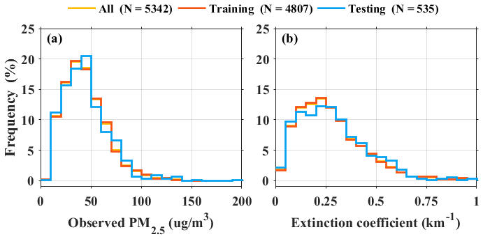
Figure 3 Probability distribution functions of all sample datasets (orange line), training dataset (red line) and testing (blue line) for observed (a) PM_2.5 and (b) EC. N represents the total number of samples of every dataset.

3.3.1 Random forest model

The RF model is a classifier that uses multiple trees to train and predict samples, which was first proposed by Breiman (2001). There is no correlation between each decision tree in the forest, and the final output of the model is jointly determined by each decision tree in the forest. RF model can handle multiple input features and provide the best outcomes by considering different features. Due to its high degree of generalization and fast training speed, the RF model is widely used in atmospheric remote sensing to solve the nonlinear fitting problem (Wei et al., 2019).

Figure 4 Mean absolute errors (MAE) between observed PM_2.5 and estimated PM_2.5 based on the (a, b) RF, (c) KNN and (d) SVM models under different tuning process.

Table 1 Summary of tuning parameters and their dynamic ranges of four different machine learning algorithms.

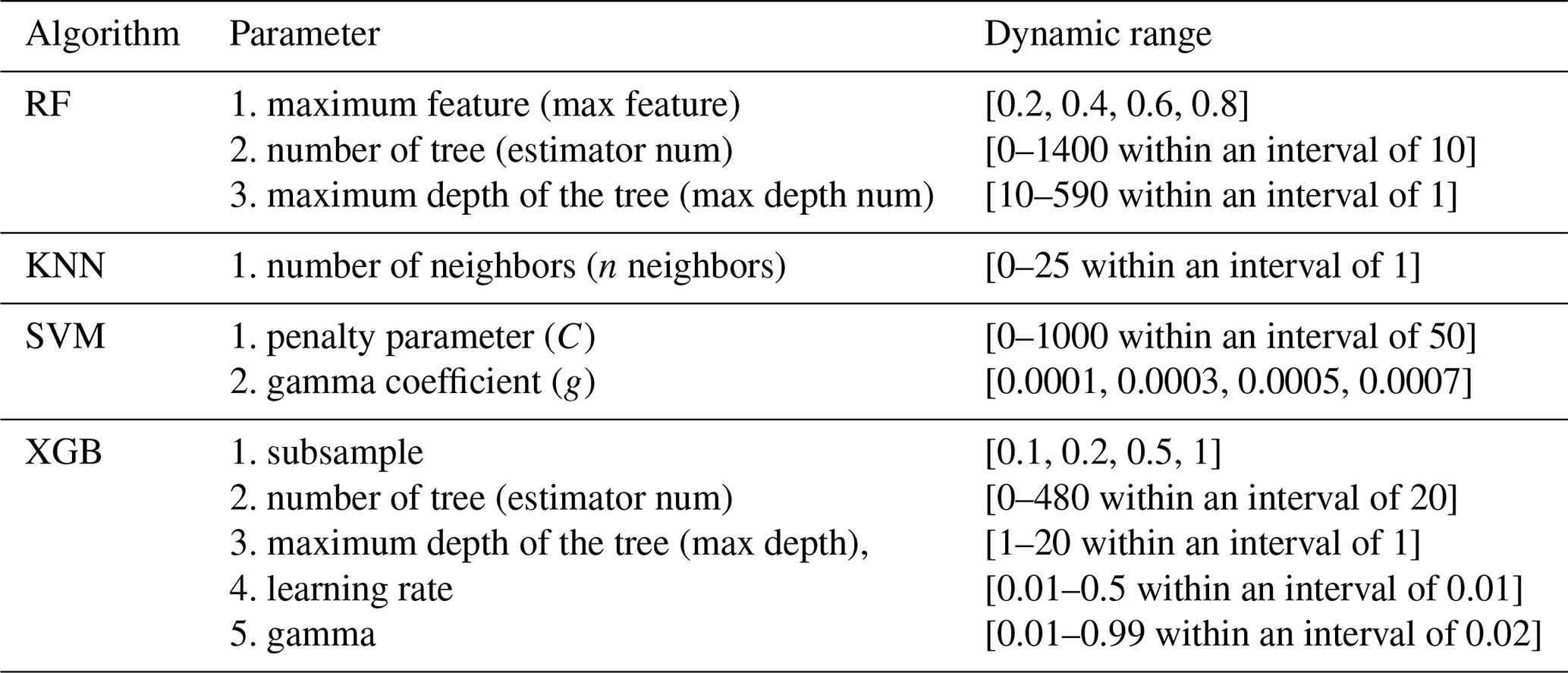
Here, the RF model was used to predict the PM_2.5 concentrations. Surface EC, RH, T, WD and WS were regarded as inputs. For the RF model, three important parameters need to be adjusted to achieve the optimal effect of the model, which include maximum feature (max feature), number of trees (estimator num) and maximum depth of the tree (max depth num), respectively (Table 1). Figure 4a and b show the parameter tuning process for estimator num and max depth num of RF model under four different max features. The max feature was set to 0.2, 0.4, 0.6 and 0.8, respectively. The results indicated that the MAE was decreased with max feature increased, while the MAE is almost unaffected when max feature is greater than 0.4. The max feature can be set to 0.4. The values of estimator num and max depth num were then defined at the minimum MAE. After parameter tuning, estimator num and the max depth num were finally defined to 1000 and 73, respectively.

3.3.2 K nearest neighbor

KNN is a ML algorithm that can be used for both classification and regression (Altman, 1992; Coomans and Massart, 1982). Its principle is to find the K training samples closest to it in the training dataset based on the distance metric for a given test sample and then make predictions based on the information of these K “neighbors”. In the atmospheric remote sensing regression task, the average value of the true values of K samples is usually used as the prediction result. Of course, the result of the weighted average based on the distance can also be used as the predicted value (Altman, 1992). The advantage of KNN is that the model can achieve good results in less training time, so it is applied to real-time analysis of some datasets. Because KNN does not require a model with parameters for training, only one parameter (number of neighbors) needs to be considered in the optimization of the KNN model. The tuning parameter process for n_neighbors of the KNN model is shown in Fig. 4c. According to the curve of MAE changing with n_neighbors, the n_neighbors can be set to 6.

3.3.3 Support vector machine

SVM is a two-class classification model, which was first proposed by Cortes and Vapnik in 1995 (Cortes and Vapnik, 1995). Its basic idea is to find a linear classifier with a separation hyperplane and maximal interval in the feature space. According to the limited sample information, the best compromise is sought between the complexity of the model (the learning accuracy of a specific training sample) and the learning ability (the ability to identify any sample without error) in order to obtain the best generalization ability (Drucker et al., 1997). It shows many unique advantages in solving small-sample, nonlinear and high-dimensional pattern recognition and can be extended to other machine learning problems such as function fitting (Cao, 2003).

For the SVM model, the penalty parameter (C) and gamma coefficient (g) need to be adjusted to achieve the optimal effect of the model. The tuning parameter process for C of the KNN model under four different g values is shown in Fig. 4d. The g was set to 0.0001, 0.0003, 0.0005 and 0.0007, respectively. Similarly, it is necessary to take an appropriate C and g value to minimize the MAE. After parameter tuning, the C and g were finally defined as 150 and 0.0005, respectively.

Figure 5 Mean absolute errors (MAE) between observed PM_2.5 and estimated PM_2.5 based on the XGB algorithms under the tuning process of (a) estimator num, (b) max depth, (c) learning rate and (d) gamma. Blue, orange, red and green lines indicate the subsample under different values.

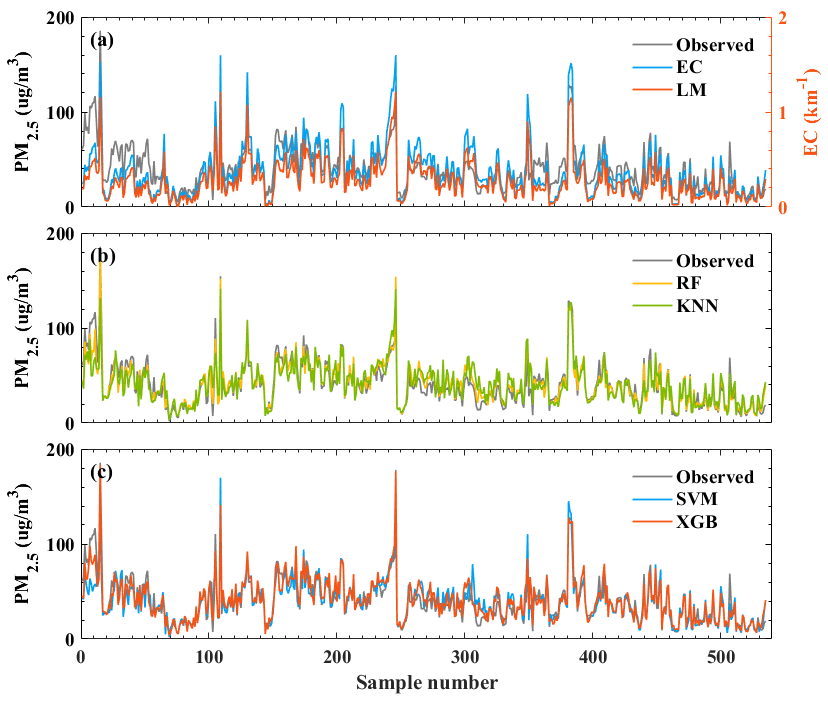
Figure 6 Variations of the estimated PM_2.5 predicted by (a) LM, (b) RF and KNN, and (c) SVM and XGB. The gray line represents the observed PM_2.5.

3.3.4 Extreme gradient boosting

XGB algorithm is an improved version of the gradient boosting decision tree (GBDT) algorithm. The GBDT algorithm is an additive model that minimizes the objective function value by gradually adding decision trees (Friedman, 2002). However, the objective function does not have a regularization term; it is just the sum of the loss function values, which may easily cause overfitting. The XGB algorithm adds a regularization term to the cost function on the basis of the GBDT algorithm and performs a second-order Taylor approximation to the objective function. Then, the exact or approximate method is used to search for the segmentation point with the highest score, and then perform the next segmentation and expand the leaf nodes (Chen et al., 2015). In this way, it is ensured that the tree structure will not be too complicated to cause overfitting in the process of minimizing the loss function. In addition, this can speed up the calculation.

To achieve the optimal effect of the XGB model, it is necessary to adjust five parameters: subsample, number of tree (estimator num), maximum depth of the tree (max depth), learning rate and gamma (Table 1). The tuning parameter process for these parameters is shown in Fig. 5. The subsample was set to 0.1, 0.2, 0.5 and 1, respectively. The results show that subsample = 1 is the most suitable. Then according to the change of the green line in each sub-panel, it is necessary to select an appropriate value to minimize the MAE. The estimator num, max depth, learning rate and gamma were finally defined to 400, 6, 0.24 and 0.01, respectively.

3.4 Calculation method of transport flux

TF is an important parameter to measure the horizontal transmission of pollutants (Y. Liu et al., 2019; Shi et al., 2020). In this study, the TF is determined by the WS and the PM_2.5 concentrations in the area under analysis. The calculation method for a certain height is shown in Eq. (5):

$$\begin{array}{}\text{(5)}& {\text{TF}}_i={\text{WS}}_i\cdot C_i,\end{array}$$

where the WS_i and C_i are the horizontal wind speed (m/s) and PM_2.5 concentrations (µg/m³) at a certain height, respectively. According to the profiles of PM_2.5 and WS, the TF profile (µg/m² s) can be obtained.

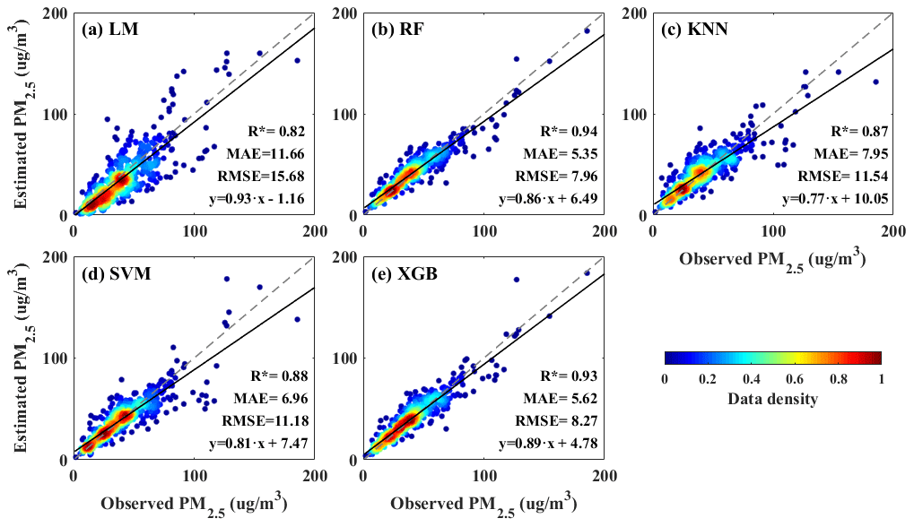
Figure 7 Correlation coefficients between observed PM_2.5 and estimated PM_2.5 based on the (a) LM, (b) RF, (c) KNN, (d) SVM and (e) XGB models. The gray and black line is the reference and regression line, respectively. The asterisk indicates that the correlation coefficient (R) passed the statistical significance difference test (P<0.05).

4 Results and discussion

4.1 Intercomparison of estimated results

In this section, the estimated PM_2.5 values of LM, RF, KMM, SVM and XGB models were compared and analyzed to evaluate the performance of these conversion models. Figure 6 shows the variation trends of EC, observed PM_2.5 and the estimated PM_2.5 by five models. The results indicated that the variation in observed PM_2.5 was similar to that in the estimated PM_2.5 of five models. However, it notes that the observed PM_2.5 and estimated PM_2.5 by LM models have a large deviation in samples 1–20. The observed PM_2.5 were larger than 100 µg/m³, while the corresponding estimated PM_2.5 of LM was less than 50 µg/m³ (Fig. 6a). This is because the estimated PM_2.5 of the LM model was directly calculated from EC, resulting in the inaccurate inversion results in some cases. These deviations are improved by machine learning models, especially in RF and XGB models (Fig. 6b and c). This is because the ML models consider the influence of meteorological factors such as RH, T, WD and WS. It can be understood that the ML models improve the prediction accuracy through meteorological factor correction. Previous studies have also pointed out that temperature and humidity correction can effectively improve the inversion accuracy of surface PM_2.5 (Zhang et al., 2015; Li et al., 2016). Zhu et al. (2021) also indicated that the performance of the RF model, which considers the effects of RH and T better than the LM model.

Figure 8 Ranking histograms of the input environment variable for (a) RF, (b) KNN, (c) SVM and (d) XGB models.

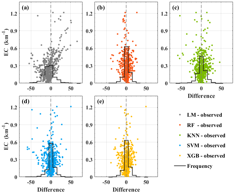
Figure 9 Difference of observed PM_2.5 and estimated PM_2.5 with the change of EC for (a) LM, (b) RF, (c) KNN, (d) SVM and (e) XGB models. The gray, red, green, blue and orange points represent the difference between LM-observed, RF-observed, KNN-observed, SVM-observed and XGB-observed PM_2.5, respectively. The black line represents the frequency.

Figure 7 shows the correlation between the observed PM_2.5 concentrations and the estimated PM_2.5 concentration predicted by the five models. The asterisk indicates that the R passed the statistical significance difference test (P<0.05). The R of LM, RF, KNN, SVM and XGB models were 0.82, 0.94, 0.87, 0.88 and 0.93, respectively. The MAE (RMSE) of these five models were 11.66 (15.68), 5.35 (7.96), 7.95 (11.54), 6.96 (11.18) and 5.62 (8.27) µg/m³, respectively. These results show that these four ML algorithms had a better fitting effect, and the error was only half of the LM error. It indicated that the performance of ML algorithms is obviously better than that of the LM algorithm. Among the four ML algorithms, RF and XGB models have similar performance, and both are better than KNN and SVM models. The RF model has the highest R and the smallest MAE. It shows that the RF model is the most suitable model for PM_2.5 inversion based on the EC.

4.2 Sensibility analysis

From the results in the previous section, the ML algorithms that take meteorological variables into account have better performance than the LM algorithm. The input variable importance analysis was performed to investigate the influence of meteorological factors, as shown in Fig. 8. For these four models, the importance ranking of the input variables (EC, WD, WS, T and RH) is the same. But there is a large difference in the importance value of each input variable. The importance values of EC in RF, KNN, SVM and XGB are 0.51, 0.87, 0.71 and 0.66, which are much larger than other input features. It indicated that the concentration of PM_2.5 was mainly affected by EC. This also proves that the surface EC and PM_2.5 have a very good linear relationship when the RH is less than 70 % (Tao et al., 2016; Lv et al., 2017). Another special point is that the importance value of RH is approximately 0.10 in RF and XGB models, while the effect of RH can be ignored in KNN and SVM models. Combined with the results in Fig. 7, it finds that the models which considered the effect of aerosol moisture absorption growth have a better performance. In addition, the effect of WS and T are also ignored in the KNN model. This leads to the performance of KNN model being weaker than the that of other three models. These results indicated that it is necessary to consider the effect of meteorological variables when using EC to retrieve PM_2.5 concentrations.

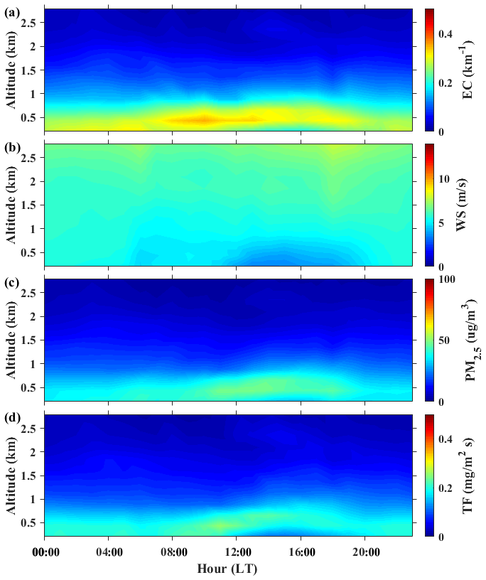
Figure 10 Hourly variations of vertical distribution of (a) EC, (b) WS, (c) PM_2.5 and (d) TF in Wuhan from January 2017 to December 2019.

Figure 9 shows the difference between estimated and observed PM_2.5 that changed with EC. The gray, red, green, blue and orange points represent the difference between LM-observed, RF-observed, KNN-observed, SVM-observed and XGB-observed PM_2.5, respectively. The black line indicates the frequency of difference. For the LM model, most of the estimated PM_2.5 is overestimated when the EC is larger than 0.6. This may be due to the fact that the LM model does not take into account the influence of humidity. The heavy pollution weather is usually accompanied by higher humidity, and the hygroscopic growth effect of aerosols cannot be ignored (Zhang et al., 2015; Liu et al., 2018b). By contrast, the difference between estimated and observed PM_2.5 is smaller in the ML models. In these four models, the frequency with a difference of less than 5 µg/m³ can reach 0.68, 0.47, 0.59 and 0.65, respectively. The frequency of difference in four ML models is similar. Moreover, the deviation of the ML models is relatively stable and does not change with the increase in EC. It also notes that although five meteorological variables are input in the ML model, not all models take into account the influence of each parameter, which leads to differences in the performance of the model. Overall, the performance of RF and XGB models are better than SVM and KNN models.

Figure 11 Seasonal and annual profiles of (a–d) PM_2.5 and (e–h) TF from January 2017 to December 2019. Corresponding color-shaded areas represent standard deviation.

4.3 Vertical evolution of PM_2.5 and TF

In this section, the diurnal and seasonal variations of TF and PM_2.5 profiles were analyzed during different periods in Wuhan. Due to the RF model having the best performance, the PM_2.5 profiles were retrieved based on the RF model.

Figure 10 shows the diurnal variation of the EC, WS, PM_2.5 and TF profiles. The daily maximum value of the EC appeared at approximately 08:00–13:00 local time (LT) in 0.4–0.6 km. The EC below 1 km has obvious diurnal characteristics, which is larger during the daytime (08:00–20:00 LT) and smaller at nighttime (Fig. 10a). By contrast, the WS below 1 km is larger during the nighttime and smaller during the daytime. The daily minimum value of WS occurred at approximately 13:00–17:00 LT in 0.2–1 km (Fig. 10b). For the diurnal variation of PM_2.5, the high PM_2.5 concentrations at nighttime are mainly concentrated below 0.5 km. After sunrise (08:00 LT), the PM_2.5 concentrations increased, and the pollution layer is higher in the vertical direction, distributed between 0.2–0.8 km. The diurnal variations of TF profiles were similar to those of PM_2.5 profiles (Fig. 10d). Near the ground, the peak TF was 0.26 mg/m² s and then remained at approximately 0.15 mg/m² s. There was an obvious conveyor belt at approximately 12:00–18:00 LT in 0.5–0.8 km. These results indicated that the transport of pollutants over Wuhan mainly occurred between 12:00 and 18:00 LT, which was similar to the results of previous studies (Ge et al., 2018; B. Liu et al., 2019).

Figure 11 shows the seasonal variation of the PM_2.5 and TF profiles. The concentration of PM_2.5 at 0.2 km has the highest value in the winter (93.7 µg/m³), followed by the autumn and summer (80.3 and 75.8 µg/m³, respectively), and lowest in the spring (53.5 µg/m³). This finding is similar to the surface observation results (Wang et al., 2016). The PM_2.5 concentration decreases gradually with the height increases. The PM_2.5 concentration decreases rapidly in the height range of 0.2 to 1 km, but the rate of reduction has obvious seasonal differences. The decline rate of the PM_2.5 in the winter and autumn is higher than that in the spring and summer. An interesting phenomenon is that the PM_2.5 mass concentrations during summer are large in the height range of 0.6 to 1.5 km. This may be caused by the transmission of dust in summer (Liu et al., 2018b, 2020). The vertical profiles of the TF are similar to those of PM_2.5 concentrations (Fig. 11e–h). The seasonal mean TF at 0.2 km is the highest in winter (0.26 mg/m² s), followed by the autumn and summer (0.2 and 0.19 mg/m² s, respectively), and lowest in spring (0.14 mg/m² s). With the height increasing, the TF profiles have obvious seasonal differences. The variations in the spring and autumn are similar; the TF gradually decreases with the height increases. In the summer (Fig. 11f), the TF is approximately 0.19 mg/m² s in the height range of 0.2 to 0.5 km and then declines above 0.5 km. The decrease rate above 0.5 km is slower than other seasons. In the winter (Fig. 11h), the TF is stable (approximately 0.26 mg/m² s) in the height range of 0.2 to 0.5 km and declines rapidly above 0.5 km. These results indicate that the transport of pollutants mainly occurs in 0.2–1 km. In general, in the autumn and winter, the TF and PM_2.5 concentrations are concentrated near the ground, indicating that local emissions are the main source of PM_2.5 (Zhang et al., 2021). In the summer, the TF is relatively high in 0.5–1.5 km, indicating that the concentration of PM_2.5 over Wuhan is affected by high-altitude dust transport (Tao et al., 2013; Liu et al., 2020). In the spring, the TF and PM_2.5 concentrations are at a low level, indicating that the air quality in Wuhan area is better in spring.

5 Summary and conclusions

This study presents a comprehensive analysis to explore the conversion of aerosol extinction coefficient to PM_2.5 concentrations based on the surface observation data from January 2014 to December 2017. The correlation and difference between observed and estimated PM_2.5 have been analyzed to evaluate the performance of LM, RF, KNN, SVM and XGB models. Furthermore, diurnal and seasonal variations of TF and PM_2.5 profiles have been investigated.

After using traditional LM and other four ML algorithms to predict the PM_2.5 mass concentrations profile, the results show that the performance of ML algorithms is better than the traditional LM algorithm. This because the ML models consider the effect of meteorological variables and can conduct the temperature and humidity correction to improve the inversion accuracy. Moreover, for the four ML algorithms, the RF model is the most suitable model for PM_2.5 estimations, followed by the XGB model; last are the SVM and KNN models. The difference in model performance is due to the difference in the decision tree structure of the model. Each ML algorithm has its own decision-making method to consider the weight of input parameters. Combined with the importance value of input variables and the deviation of results, the results indicated that the higher the weight of the meteorological parameters in the model, the smaller the deviation of the results. Finally, the diurnal and seasonal variations of TF and PM_2.5 profiles were analyzed. For diurnal variations, the high PM_2.5 concentrations at nighttime are mainly concentrated below 0.5 km. During the daytime, the pollution layers are usually suspended in the higher altitude and are distributed between 0.2–0.8 km. The high TF appeared at approximately 12:00–18:00 LT in 0.5–0.8 km. These results indicated that the transport of pollutants over Wuhan mainly occurred between 12:00 and 18:00 LT. For seasonal variations, the TF and PM_2.5 mass concentrations are concentrated near the ground in autumn and winter, indicating that local emissions are the main source of PM_2.5 during these periods. In the summer, TF has a relatively high value in 0.5–1.5 km, which indicates the concentration of PM_2.5 over Wuhan is affected by high-altitude dust transport.

Our work comprehensively compares the performance of LM, RF, KNN, SVM and XGB models. From the perspective of correlation and deviation between observed and estimated PM_2.5, we conclude that the performances of the RF and XGB models are better than others, followed by the SVM and KNN models, and finally the LM model. This information can provide us with a reference to apply lidar data in air quality research.