Spatial distributions of X_CO2 seasonal cycle amplitude and phase over northern high-latitude regions

Satellite-based observations of atmospheric carbon dioxide (CO₂) provide measurements in remote regions, such as the biologically sensitive but undersampled northern high latitudes, and are progressing toward true global data coverage. Recent improvements in satellite retrievals of total column-averaged dry air mole fractions of CO₂ ($X_{{\mathrm{CO}}_{\mathrm{2}}}$) from the NASA Orbiting Carbon Observatory 2 (OCO-2) have allowed for unprecedented data coverage of northern high-latitude regions, while maintaining acceptable accuracy and consistency relative to ground-based observations, and finally providing sufficient data in spring and autumn for analysis of satellite-observed $X_{{\mathrm{CO}}_{\mathrm{2}}}$ seasonal cycles across a majority of terrestrial northern high-latitude regions. Here, we present an analysis of $X_{{\mathrm{CO}}_{\mathrm{2}}}$ seasonal cycles calculated from OCO-2 data for temperate, boreal, and tundra regions, subdivided into 5^∘ latitude by 20^∘ longitude zones. We quantify the seasonal cycle amplitudes (SCAs) and the annual half drawdown day (HDD). OCO-2 SCAs are in good agreement with ground-based observations at five high-latitude sites, and OCO-2 SCAs show very close agreement with SCAs calculated for model estimates of $X_{{\mathrm{CO}}_{\mathrm{2}}}$ from the Copernicus Atmosphere Monitoring Services (CAMS) global inversion-optimized greenhouse gas flux model v19r1 and the CarbonTracker2019 model (CT2019B). Model estimates of $X_{{\mathrm{CO}}_{\mathrm{2}}}$ from the GEOS-Chem CO₂ simulation version 12.7.2 with underlying biospheric fluxes from CarbonTracker2019 (GC-CT2019) yield SCAs of larger magnitude and spread over a larger range than those from CAMS, CT2019B, or OCO-2; however, GC-CT2019 SCAs still exhibit a very similar spatial distribution across northern high-latitude regions to that from CAMS, CT2019B, and OCO-2. Zones in the Asian boreal forest were found to have exceptionally large SCA and early HDD, and both OCO-2 data and model estimates yield a distinct longitudinal gradient of increasing SCA from west to east across the Eurasian continent. In northern high-latitude regions, spanning latitudes from 47 to 72^∘ N, longitudinal gradients in both SCA and HDD are at least as pronounced as latitudinal gradients, suggesting a role for global atmospheric transport patterns in defining spatial distributions of $X_{{\mathrm{CO}}_{\mathrm{2}}}$ seasonality across these regions. GEOS-Chem surface contact tracers show that the largest $X_{{\mathrm{CO}}_{\mathrm{2}}}$ SCAs occur in areas with the greatest contact with land surfaces, integrated over 15–30 d. The correlation of $X_{{\mathrm{CO}}_{\mathrm{2}}}$ SCA with these land surface contact tracers is stronger than the correlation of $X_{{\mathrm{CO}}_{\mathrm{2}}}$ SCA with the SCA of CO₂ fluxes or the total annual CO₂ flux within each 5^∘ latitude by 20^∘ longitude zone. This indicates that accumulation of terrestrial CO₂ flux during atmospheric transport is a major driver of regional variations in $X_{{\mathrm{CO}}_{\mathrm{2}}}$ SCA.

1 Introduction

The changing climate influences carbon exchange in every ecosystem on the planet, and polar amplification is driving more rapid changes at higher latitudes (Smith et al., 2019; Park et al., 2018; Pithan and Mauritsen, 2014; Holland and Bitz, 2003; Manabe and Wetherald, 1975). An understanding of the rapidly changing carbon dynamics at high northern latitudes is necessary to improve our understanding of global carbon exchange. However, despite the apparent importance of northern high-latitude regions in quantifying the global carbon budget, Bradshaw and Warkentin (2015) point out that a great deal of uncertainty remains in the spatial patterns of carbon stocks and fluxes in boreal forest regions, and their results from predictive climate models show that the boreal forest may eventually shift from a carbon sink to a carbon source. Euskirchen et al. (2017), Barlow et al. (2015), and Pan et al. (2011) all point out that a shortage of observations in boreal forest regions is a major impediment to understanding global carbon uptake, motivating further exploration of alternative data sources, such as satellite measurements. Since pioneering work by Thoning et al. (1989), analysis of the seasonal cycles of atmospheric CO₂ concentrations has been widely used to evaluate carbon exchange dynamics, and the amplitude of the regular seasonal oscillations in atmospheric CO₂ concentrations is a common metric used to infer relative CO₂ uptake. Many studies have combined process-based and atmospheric transport modeling with in situ and airborne observations to infer long-term temporal trends and spatial distributions of seasonal CO₂ exchange and concluded that boreal forest regions play an essential role in global carbon dynamics (Lin et al., 2020; Yin et al., 2018; Piao et al., 2017; Barlow et al., 2015; Bradshaw and Warkentin, 2015; Gauthier et al., 2015; Graven et al., 2013; Pan et al., 2011; Tans et al., 1990). Lin et al. (2020) compared seasonal cycle amplitudes (SCAs) from surface in situ measurements of CO₂ to those estimated from GEOS-Chem transport modeling coupled with CAMS v17r1 flux estimates and found that Siberia had the largest SCA of any region considered when normalized for area. Furthermore, Lin et al. (2020) found that even though Siberia is a relatively small source region, fluxes from Siberia were the second most influential in determining SCA of in situ CO₂ on a global scale, following those from Northern Hemisphere midlatitudes.

It has been well established that the SCA of atmospheric CO₂ increases with latitude in the Northern Hemisphere due to the increased seasonal attenuation of sunlight which drives more extreme seasonality in temperature and ecosystem productivity at higher latitudes. There is general consensus that this latitudinal gradient in SCA is increasing over time, so that while CO₂ SCAs are increasing across the Northern Hemisphere, the SCAs at higher northern latitudes are increasing at an accelerated rate. There is still some controversy regarding what mechanisms are driving changes in CO₂ SCA and how spatial distributions or temporal trends in CO₂ seasonality are influenced by atmospheric transport patterns or regional changes in carbon exchange. Recent work by Liu et al. (2020) suggests that global increases in CO₂ SCA since the 1960s are a result of increases in growing season mean temperatures, and polar amplified warming would then explain the increase in the latitudinal gradients in SCA. Studies by Piao et al. (2017), Forkel et al. (2016), and Graven et al. (2013) used global models to show that increasing latitudinal gradients in SCA are driven by the ecological effects of climate change and changes in vegetation, primarily suggesting CO₂ fertilization as the dominant mechanism. This point is confirmed by findings from Bastos et al. (2019) that attribute enhanced SCA in boreal Asia and Europe to increases in net biome productivity as a result of CO₂ fertilization. Although they do not address the increase in latitudinal gradients over time, Zeng et al. (2014) and Gray et al. (2014) argue that agricultural expansion in the Northern Hemisphere midlatitudes has resulted in increases in seasonal carbon exchange, which, in turn, result in larger SCA of CO₂ concentrations on a global scale. Barnes et al. (2016) suggest that it is actually the temperate forest between 30 and 50^∘ N that is the dominant driver of seasonal carbon exchange on global scales. Yet another study by Yin et al. (2018) found evidence that challenged previous assumptions about the relationship between seasonal cycle amplitude and spring and autumn temperatures in northern high latitudes, emphasizing the need for continued data-driven model validation for these regions. Despite their disagreements, most agree that the seasonality in atmospheric CO₂ at northern high latitudes, and specifically the boreal forest, requires continued attention as carbon dynamics continue to change. While this paper does not consider temporal changes in SCA, an assessment of spatial distributions of SCA implied by satellite-based observations over northern high-latitude terrestrial regions can provide a good foundation for exploring temporal changes in these spatial distributions in later analyses.

Satellite-based infrared spectrometers like the NASA Orbiting Carbon Observatory 2 (OCO-2) (O'Dell et al., 2018; Wunch et al., 2017; Crisp et al., 2017), SCIAMACHY (Reuter et al., 2011; Bovensmann et al., 1999; Burrows et al., 1995), and GOSAT (Basu et al., 2013; Yoshida et al., 2013; Hamazaki et al., 2005) provide global measurements of column-averaged dry air mole fractions of CO₂ ($X_{{\mathrm{CO}}_{\mathrm{2}}}$) and particularly can quantify $X_{{\mathrm{CO}}_{\mathrm{2}}}$ in remote, un-instrumented regions. Retrievals and instrument technologies have been advancing rapidly, and boreal-forest-specific methods of $X_{{\mathrm{CO}}_{\mathrm{2}}}$ bias correction and quality control filtering have been developed and validated where ground truth exists (Jacobs et al., 2020; Kiel et al., 2019; O'Dell et al., 2018). In addition, the development of collaborative networks of ground-based solar-viewing spectrometers, including the Total Carbon Column Observing Network (TCCON) and the Collaborative Carbon Column Observing Network (COCCON), has provided a framework for robust global validation of similar passive satellite-based observations (Frey et al., 2019; Wunch et al., 2011). These combined efforts of satellite-based and ground-based total atmospheric column measurements of CO₂ offer a wealth of opportunities for gaining insights into the global climate system as a whole.

In this paper, we quantify and analyze seasonal cycle parameters derived directly from satellite-based observations of $X_{{\mathrm{CO}}_{\mathrm{2}}}$, across the northern high-latitude terrestrial regions. This work represents progress in the application of global monitoring of atmospheric CO₂ to the continued evaluation of global-scale carbon dynamics and shows how satellites like OCO-2 can be used to monitor CO₂ biospheric exchange. In this analysis, OCO-2 data over terrestrial northern high latitudes are used to explore spatial distributions of seasonal cycle amplitude (SCA) and seasonal cycle phase. Interpretation of these spatial distributions can be used to test previous claims and provide new insights into what is driving carbon exchange at northern high latitudes. In particular, we explore how seasonality in $X_{{\mathrm{CO}}_{\mathrm{2}}}$ differs for the North American, European, and Asian boreal forest regions and how the boreal forest fits within the broader context of northern high-latitude regions. In addition, seasonal cycle parameters derived from OCO-2 observations are combined with those from ground-based TCCON and COCCON observations and then compared with seasonal cycle parameters from three model frameworks: the Copernicus Atmospheric Monitoring Services (CAMS) global inversion-optimized greenhouse gas flux model estimates of $X_{{\mathrm{CO}}_{\mathrm{2}}}$ (Chevallier, 2020b), with in situ data assimilation; CarbonTracker2019 posterior $X_{{\mathrm{CO}}_{\mathrm{2}}}$ estimates (CT2019B; Jacobson et al., 2020a); and the GEOS-Chem CO₂ simulation (Nassar et al., 2010) with underlying biospheric fluxes from CarbonTracker2019 (GC-CT2019). Ultimately, we use simulations of GEOS-Chem surface contact tracers and flux estimates from CAMS and CarbonTracker2019, as well as estimates of fossil fuel emissions from the Community Emissions Data System (CEDS; Hoesly et al., 2018) and estimates of biomass burning emissions from the Global Fire Emissions Database, version 4.1 (GFED4.1s; Randerson et al., 2018; van der Werf et al., 2017), to address the question of how much spatial variability in $X_{{\mathrm{CO}}_{\mathrm{2}}}$ seasonal cycle parameters may be attributed to magnitudes of fluxes within the observation zones and how much may be attributed to the regional- and continental-scale accumulation of CO₂ fluxes during atmospheric transport.

2 Methods

2.1 OCO-2 data

The NASA Orbiting Carbon Observatory 2 (OCO-2) launched in 2014 and began collecting data in September of that year. Daily averages of $X_{{\mathrm{CO}}_{\mathrm{2}}}$ are calculated for each zone using observations from OCO-2 Lite files (version 9, “B9”; OCO-2 Science Team/Michael Gunson, Annmarie Eldering, 2018). Ongoing improvements in the ACOS retrieval algorithm and previous efforts by Jacobs et al. (2020) to develop quality control thresholds tailored to OCO-2 B9 retrievals over boreal forest regions (boreal QC) have allowed sufficient data over our 5^∘ latitude by 20^∘ longitude zones to construct $X_{{\mathrm{CO}}_{\mathrm{2}}}$ time series that yield robust seasonal cycle parameterization. The boreal QC was evaluated for use with terrestrial OCO-2 B9 retrievals north of 50^∘ N (Jacobs et al., 2020), and the zones considered here cover the majority of land north of 50^∘ N. The southern boundaries of the southernmost zones of North America are at 47^∘ N, but the 3^∘ of latitude is not expected to significantly impact the effectiveness of the boreal QC filtering. Instead of the standard B9 bias correction, we use a modified bias correction that includes temperature at 700 hPa (T700), as discussed by Jacobs et al. (2020), because it was found in previous results to reduce the seasonality of OCO-2 bias relative to ground-based TCCON and EM27/SUN measurements. Seasonal cycle fits to OCO-2 retrievals of $X_{{\mathrm{CO}}_{\mathrm{2}}}$ with the standard B9 bias correction, as well as fits to OCO-2 B10 retrievals, were also calculated and compared to model-derived seasonal cycle fits in the Supplement (see Sect. S2). The spatial distribution of seasonal cycle parameters across northern high-latitude regions is similar for all three types of OCO-2 retrievals, but the alternative bias correction yields improved agreement with model-derived seasonal cycle parameters.

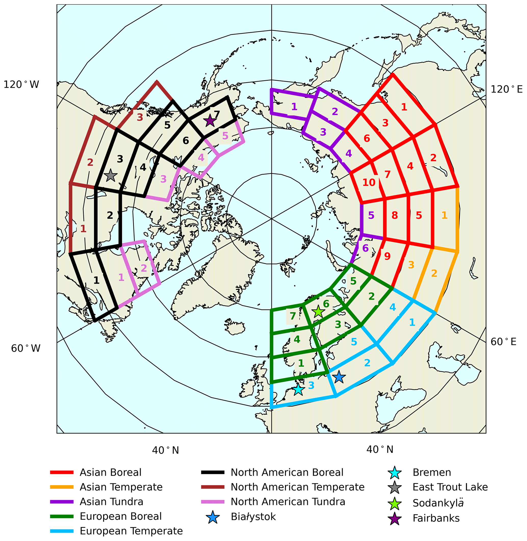
Figure 1 Map for of regions, zones, and locations of ground-based $X_{{\mathrm{CO}}_{\mathrm{2}}}$ observations.

2.2 TCCON and EM27/SUN data

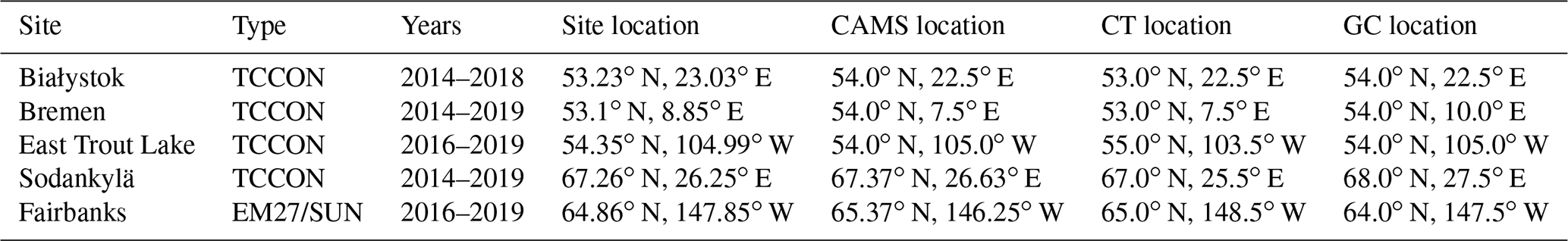
The Total Carbon Column Observing Network (TCCON) is a ground-based network of sites observing $X_{{\mathrm{CO}}_{\mathrm{2}}}$ using high-spectral-resolution solar-viewing Fourier transform infrared spectrometers (FTSs). Data are included from four TCCON sites: East Trout Lake, Canada, in North American boreal zone 3 (Wunch et al., 2018); Sodankylä, Finland, in European boreal zone 6 (Kivi et al., 2014; Kivi and Heikkinen, 2016); Białystok, Poland, in European temperate zone 2 (Deutscher et al., 2019); and Bremen, Germany, in European temperate zone 3 (Notholt et al., 2019) (see site details in Table 1 and locations mapped in Fig. 1). The Collaborative Carbon Column Observing Network (COCCON) is a network of sites observing with the Bruker EM27/SUN FTS (Gisi et al., 2012), which are lower-resolution mobile solar-viewing spectrometers that serve as complement to TCCON measurements. EM27/SUN observations have been compared to TCCON observations in multiple studies, most notably Sha et al. (2020), Tu et al. (2020), Frey et al. (2019), Velazco et al. (2018), and Hedelius et al. (2017). In most of these comparisons EM27/SUN and TCCON observations agree with biases less than 0.25 ppm on average. In some cases offsets between EM27/SUN and TCCON observations are reported to be as large as 2 ppm, but the proven stability of the EM27/SUN should allow for a bias correction that would yield good agreement between TCCON and EM27/SUN retrievals. The EM27/SUN instruments have measured $X_{{\mathrm{CO}}_{\mathrm{2}}}$ in a number of campaigns to validate OCO-2 and other satellite-based observations, including work by Jacobs et al. (2020), Velazco et al. (2018), and Klappenbach et al. (2015), suggesting good agreement between EM27/SUN observations and satellite-based observations. In this analysis, observations with an EM27/SUN FTS in Fairbanks, Alaska, USA (65.859^∘ N, 147.850^∘ W; Jacobs et al., 2021), are used as a fifth ground-based comparison in the boreal forest. Fairbanks is an established COCCON site as of 2018, so the instrument participates regularly in performance and calibration checks at the central facility operated by KIT, and data processed in compliance with COCCON recommendations are available. In this study, we use the GGG2014 retrieval algorithm coupled with the EM27/SUN GGG interferogram processing suite (EGI; Hedelius and Wennberg, 2017) instead of the standard COCCON retrieval methods for consistency with TCCON retrievals and because this data product has already been bias corrected to TCCON using side-by-side observations at Caltech, as described in detail by Jacobs et al. (2020). Seasonal cycle fits for ground-based observations at these five sites use daily averages of retrievals collected within 2 h of local solar noon, weighted by retrieval error, as described by Jacobs et al. (2020). We refer to these daily averages as near-noon ground-based (NNG) observations, and this time frame is chosen because OCO-2 overpasses tend to occur within approximately 1 h of local solar noon over these northern high-latitude regions.

Table 1 Summary of instrument type, years of observations, geographic coordinates, and corresponding coordinates of the nearest model grid point in CAMS, CT2019B (CT), and GC-CT2019 (GC) for each ground site.

2.3 Regions and zones

We define regions in North America, Europe, and Asia, which are further subdivided into 5^∘ latitude by 20^∘ longitude zones, and zones are designated as temperate, boreal, or tundra. For the purposes of this analysis, the classification of zones as temperate, boreal, or tundra, as well as the longitudinal division between the European and Asian regions, are guided by maps of ecoregions from Hayes et al. (2011) and Euskirchen et al. (2007) (see Fig. 1). The boreal forest zones considered cover a narrower range of latitudes than the boreal regions defined for the Transcom 3 ecoregions (Gurney et al., 2000), which include all high Arctic tundra and portions of temperate Asia as part of the boreal regions. Otherwise, the North American boreal region and Eurasian boreal region defined by Transcom 3 are very similar to the North American boreal and Asian boreal regions defined in this analysis. We differ markedly from Transcom 3 in defining separate European boreal and European temperate regions, while Transcom 3 combines all of Europe into a single European region. In North America, the zones are shifted by 3^∘ latitude relative to the zones in Eurasia – starting at 47^∘ N and extending in to 72^∘ N in 5^∘ increments. This was done to bring ground sites in the North American boreal region closer to the center latitude of their encompassing zones and to more accurately fit the boundaries of temperate, boreal, and tundra biomes.

Also shown in Fig. 1 are the locations of five ground sites where long-term observations of $X_{{\mathrm{CO}}_{\mathrm{2}}}$ have been collected (see Table 1 for details). These ground sites include two sites in the European temperate region (Białystok and Bremen), one site in the European boreal region (Sodankylä), and two sites in the North American boreal region (East Trout Lake and Fairbanks). Ground-based data are explained further in Sect. 2.2, and seasonal cycles of ground-based data are compared to satellite and model-derived seasonal cycles in Sect. 3.1.

2.4 $X_{{\mathrm{CO}}_{\mathrm{2}}}$ seasonal cycle modeling and parameters

The primary focus of our analysis is characterizing seasonality in $X_{{\mathrm{CO}}_{\mathrm{2}}}$ and exploring how and why this seasonality differs across northern high-latitude regions, with particular emphasis on the boreal forest. To this end, time series are constructed using daily averaged $X_{{\mathrm{CO}}_{\mathrm{2}}}$ from satellite retrievals, ground-based solar-viewing Fourier transform infrared (FTIR) spectrometers, and model estimates (see previous methods sections for details). Seasonal cycles are characterized following methods used by Lindqvist et al. (2015), in which daily $X_{{\mathrm{CO}}_{\mathrm{2}}}$ values are fit to a skewed sine wave of the form

$$\begin{array}{}\text{(1)}& \begin{array}{rl}f\left(t\right)& =a_{\mathrm{0}}+a_{\mathrm{1}}t+a_{\mathrm{2}}\sin \left(\mathit{\omega }\right[t-a_{\mathrm{3}}]\\ & +{\cos }^{-\mathrm{1}}\left[a_{\mathrm{4}}\cos \right(\mathit{\omega }[t-a_{\mathrm{5}}]\left)\right]),\end{array}\end{array}$$

where t is days, $\mathit{\omega }=\frac{\mathrm{2}\mathit{\pi }}{\mathrm{365.25}}$, the interannual trend is defined by a₀+a₁t, and the seasonal cycle amplitude (SCA) is defined by $\mathrm{2}\left|a_{\mathrm{2}}\right|$. As a metric for seasonal timing we define half drawdown day (HDD) as the day of year when the detrended seasonal cycle fit, $f\left(t\right)-a_{\mathrm{0}}-a_{\mathrm{1}}t$, crosses zero from positive to negative. The fit is calculated using nonlinear least squares optimization with the standard error, σ, defined as the mean of daily standard deviations in $X_{{\mathrm{CO}}_{\mathrm{2}}}$ over all days in the time series. If there is no daily standard deviation, as is the case with single point model estimates near ground sites from the CT2019B and GC-CT2019 models, the standard error is assumed to be 0.25 ppm. Specifically, we implement the Levenberg–Marquardt algorithm for nonlinear least squares fitting, which seeks to minimize the quantity,

$$\begin{array}{}\text{(2)}& {\mathit{\chi }}^{\mathrm{2}}=\sum _{i=\mathrm{1}}^n{\displaystyle \frac{{\left[y_i-f(x_i,a_o,a_{\mathrm{1}},\mathrm{\dots }{a}_j)\right]}^{\mathrm{2}}}{{\mathit{\sigma }}^{\mathrm{2}}}},\end{array}$$

and yields variance for each parameter in the fit equation given by

$$\begin{array}{}\text{(3)}& {\mathit{\sigma }}_{a_j}^{\mathrm{2}}=\left(\right[{\mathbf{J}}^T\mathbf{WJ}{]}^{-\mathrm{1}}{)}_{jj},\end{array}$$

where J is the Jacobian and $\mathbf{W}={\mathbf{V}}_{x_i}^{-\mathrm{1}}$, the inverse of the covariance matrix. In this case uncertainties are scaled by χ², such that ${\mathbf{V}}_{x_i}$ is defined as χ²σ²I. The variance in fit parameters is taken to be a direct estimate of fit uncertainty and translate to uncertainty in SCA, defined as $\mathrm{2}{\mathit{\sigma }}_{a_{\mathrm{2}}}$ and depicted in figures as error bars, where appropriate.

The seasonal cycle fitting approach used by Lindqvist et al. (2015) was found to be more numerically stable than fitting to a truncated Fourier series, as has been employed in previous studies (Wunch et al., 2013; Thoning et al., 1989), because periods of missing data can produce unrealistic oscillations in a fit to a truncated Fourier series. Even in cases with continuous data, the fit to a truncated Fourier series can yield unrealistic oscillations within the overall seasonal cycle that do not appear to accurately depict variability in the data. These unrealistic oscillations are more pronounced when there are gaps in the time series of data. The fits to Eq. (1) also show a degradation of the seasonal cycle shape with larger gaps in the time series but yield more stability in fitting time series with some data gaps than the fits to a truncated Fourier series. This is an important consideration for high-latitude regions, which have winter gaps in observations for most passive atmospheric remote sensing measurements, due to lower solar elevation angles or night at satellite overpass time (near solar noon).

2.5 CAMS model estimates

Model estimates of $X_{{\mathrm{CO}}_{\mathrm{2}}}$ from the Copernicus Atmospheric Monitoring Services (CAMS) global inversion-optimized greenhouse gas flux model v19r1 are used here as a model comparison to OCO-2 and NNG data. The modeling framework for CAMS CO₂ flux inversions is described in detail by Chevallier (2020b). Quality assessments for the Northern Hemisphere by Chevallier (2020a) report that nearly all biases in both CAMS estimates of in situ CO₂ relative to unassimilated aircraft observations and CAMS estimates of $X_{{\mathrm{CO}}_{\mathrm{2}}}$ relative to TCCON observations are within 1 ppm, with standard deviation in bias around 2 ppm. CAMS estimates of $X_{{\mathrm{CO}}_{\mathrm{2}}}$ are available as 3-hourly estimates with 1.9^∘ latitude by 3.75^∘ longitude spatial resolution, which is sufficient for providing multiple grid points within each zone and coincidence with most ground sites within approximately 100 km (see Table S1 in the Supplement for exact coordinates of grid points nearest to the ground sites). Daily averages and standard deviation in CAMS $X_{{\mathrm{CO}}_{\mathrm{2}}}$, used to calculate seasonal cycle fits, are taken from combined spatial aggregations within zones or coincidence regions and temporal aggregations for each 24 h date in UTC. We use CAMS model estimates with data assimilation from a global network of surface in situ observations at 119 locations but without any satellite data assimilation. In addition to the $X_{{\mathrm{CO}}_{\mathrm{2}}}$ estimates, the CAMS model output includes surface flux estimates, which will be considered further in the Discussion, Sect. 4.2. Both CAMS flux estimates and CAMS $X_{{\mathrm{CO}}_{\mathrm{2}}}$ estimates use the same atmospheric transport modeling framework.

2.6 CarbonTracker2019 model estimates

The CarbonTracker2019 (CT2019) model is an inverse model that provides estimates of global CO₂ fluxes with a 1^∘ by 1^∘ spatial resolution and estimates of global $X_{{\mathrm{CO}}_{\mathrm{2}}}$ fields with a atmospheric transport simulated by the TM5 model (Krol et al., 2005) with a spatial resolution of 2^∘ latitude by 3^∘ longitude (Jacobson et al., 2020a, b). The model assimilates in situ measurements of atmospheric CO₂ concentrations from aircraft, AirCore (Karion et al., 2010), tall tower, and surface measurement platforms at 460 sites around the world. For CT2019 fluxes considered in this analysis and used in GEOS-Chem simulations, we use the original CT2019 release from May 2020 (Jacobson et al., 2020a), but for the posterior estimates of $X_{{\mathrm{CO}}_{\mathrm{2}}}$ we use results from an updated release, CT2019B (Jacobson et al., 2020b). This was a matter of practical necessity because of the timing of the updated CT2019B release and the fact that $X_{{\mathrm{CO}}_{\mathrm{2}}}$ estimates from the previous CT2019 version were unavailable after this release. The purpose of the release of CT2019B was reported as “Correction of a minor bug in CT2019” (Jacobson et al., 2020b). CT2019 uses the Global Fire Emissions Database, version 4.1 (GFED4.1s; Randerson et al., 2018; van der Werf et al., 2017), as one part of the fire module that estimates emissions from biomass burning, while fossil fuel emissions are driven by a combination of the Miller emissions inventory (see Jacobson et al., 2020b, for more details) and the Open-Data Inventory for Anthropogenic Carbon dioxide (ODIAC; Oda and Maksyutov, 2011) emissions datasets. Biospheric exchange is driven by the Carnegie-Ames-Stanford Approach (CASA) biogeochemical model introduced by Potter et al. (1993). In this analysis we calculate seasonal cycle fits using daily CT2019B posterior $X_{{\mathrm{CO}}_{\mathrm{2}}}$ and compare these to corresponding seasonal cycle fits from ground-based and satellite-based observations. The CT2019 estimates of biospheric CO₂ exchange are also used within a GEOS-Chem model framework, described in Sect. 2.7, and considered in an assessment of the role of fluxes in shaping $X_{{\mathrm{CO}}_{\mathrm{2}}}$ seasonality.

2.7 GEOS-Chem CO₂ and transport tracer simulations

The GEOS-Chem atmospheric transport model version 12.7.2 (more detailed information at https://geos-chem.seas.harvard.edu/, last access: 31 July 2020) has 2^∘ latitude by 2.5^∘ longitude spatial resolution, using MERRA-2 meteorology (Gelaro et al., 2017). We use the GEOS-Chem CO₂ simulation (Nassar et al., 2010) and GEOS-Chem surface contact tracers, for 2014–2016, to examine the relationships between seasonal cycle parameters and atmospheric transport patterns and speculate on the role of atmospheric transport in determining spatial distributions of $X_{{\mathrm{CO}}_{\mathrm{2}}}$ seasonality across northern high latitudes. The GEOS-Chem CO₂ simulation provides daily $X_{{\mathrm{CO}}_{\mathrm{2}}}$ estimates and source attributions for total column CO₂, with biospheric fluxes for land and ocean taken from the CT2019 model (Jacobson et al., 2020a), so we refer to this combination of GEOS-Chem atmospheric transport and CT2019 biospheric exchange as GC-CT2019 throughout this paper. Similar to CT2019, this GC-CT2019 simulation uses GFED4.1 to estimate emissions from biomass burning, but unlike CT2019, it uses the Community Emissions Data System (CEDS; Hoesly et al., 2018) for fossil fuel emissions and results from Bukosa et al. (2021) for the chemical production of CO₂ in the atmosphere. For the fossil fuel emissions, the CEDS inventory ended in 2014, so 2015 and 2016 emissions were scaled by the CEDS 2014 emissions to match the global total in those later years, as reported by ODIAC. We used this approach, rather than using ODIAC alone, because the CEDS inventory includes anthropogenic biofuel emissions that are not in ODIAC. The GC-CT2019 simulation is initialized on 1 January 2007 with observed global ocean surface mean CO₂ (Dlugokencky and Tans, NOAA/GML, http://www.esrl.noaa.gov/gmd/ccgg/trends/, last access: 15 December 2020), giving the model 7 years of spin-up before generating the output for 2014–2016 used here. GC-CT2019 estimates, like CT2019B posterior $X_{{\mathrm{CO}}_{\mathrm{2}}}$ estimates, are obtained as daily values for grid points with daily averages and standard deviation calculated spatially for each 5^∘ latitude by 20^∘ longitude zone or 5^∘ latitude by 10^∘ longitude satellite coincidence region; there is no temporal averaging performed on these estimates for this analysis. Unlike the CAMS model and CT2019B $X_{{\mathrm{CO}}_{\mathrm{2}}}$ estimates, which provide optimized CO₂ flux, and $X_{{\mathrm{CO}}_{\mathrm{2}}}$ estimates using internally consistent atmospheric transport models, GC-CT2019 uses CT2019 fluxes that are estimated using TM5 to simulate atmospheric transport rather than the GEOS-Chem transport model. In addition, the fossil fuel and biomass burning flux estimates used in GC-CT2019 are based on slightly different source datasets. GEOS-Chem simulations are run for 2014–2016 rather than for 2014–2019, like the OCO-2 observations and other model estimates. The analysis shown in the Supplement (see Fig. S39) suggests that the spatial distributions of SCA and HDD across northern high-latitude zones are not likely to significantly change for CAMS, CT2019B, or OCO-2 when calculated for 2014–2016 instead of 2014–2019. In particular, changes in SCA for the different time periods are less than approximately 0.5 ppm, which represents less than 10 % of the ∼5 ppm variability in SCA across these northern high-latitude regions. There are some larger discrepancies between OCO-2 HDD for 2014–2016 and OCO-2 HDD for 2014–2019, with a couple of zones yielding a difference of around 8 d, but this may be partially attributed to the fact that some zones lack sufficient data points in the 2014–2016 time period for a stable and accurate seasonal phase determination.

To examine the role of atmospheric transport in shaping the seasonal cycle of $X_{{\mathrm{CO}}_{\mathrm{2}}}$, we define new tracers of air mass surface contact in the GEOS-Chem atmospheric transport model. These surface contact tracers are emitted uniformly and continuously over specific surface types at a rate of 1 molecule m⁻² s⁻¹, transported like CO₂ and other constituents, and decay with a prescribed e-fold lifetime. One set of these surface contact tracers is emitted uniformly over the ocean and another set is emitted uniformly over land. For both surfaces, we release multiple tracers with lifetimes of 5, 15, 30, and 90 d, making eight surface contact tracers in total. After spinning up the simulation for several e-fold lifetimes, the tracer concentration at a point in the model indicates the integrated upwind contact with land or ocean over the timescale of the tracer lifetime. For example, high concentrations of the land surface contact tracers reveal locations where atmospheric circulations have confined air over continents. These surface contact tracers are like e90 (Prather et al., 2011), except that e90 is emitted uniformly from all surfaces and therefore indicates upwind contact with any surface rather than particular surface types as we have done. The sum of our land and ocean tracers with 90 d lifetimes is equal to e90. The surface contact tracers are initialized and run for the same periods as the GC-CT2019 simulation, 2014–2016. The surface contact tracers for a given zone were found to vary minimally in time, so a total zonal average of surface contact tracer contributions was taken spatially and temporally within each zone (see map in Fig. 1) and over all days in 2014–2016.

2.8 Treatment of CO₂ flux estimates

The role of fluxes in determining $X_{{\mathrm{CO}}_{\mathrm{2}}}$ seasonality at northern high latitudes is assessed using flux estimates from CAMS, as well as the sum of CO₂ flux estimates from the CEDS and GFED4.1s inventories (Hoesly et al., 2018; Randerson et al., 2018; van der Werf et al., 2017) and CarbonTracker2019 biospheric fluxes from land and ocean (Jacobson et al., 2020a) used to generate the GC-CT2019 $X_{{\mathrm{CO}}_{\mathrm{2}}}$ estimates. While the CAMS v19r1 and CT2019B model frameworks have internally consistent atmospheric transport because both CO₂ flux and $X_{{\mathrm{CO}}_{\mathrm{2}}}$ estimates are generated using the same atmospheric transport model (Chevallier, 2020b; Jacobson et al., 2020a), GC-CT2019 includes biospheric fluxes from CarbonTracker2019 using the TM5 transport model but then applies GEOS-Chem atmospheric transport modeling to estimate $X_{{\mathrm{CO}}_{\mathrm{2}}}$. In addition, the fossil fuel fluxes from CEDS and biomass burning fluxes from GFED4.1s may include other assumptions about atmospheric transport.

First, CO₂ fluxes from each model are averaged spatially within each 5^∘ latitude by 20^∘ longitude zone (see Fig. 1) for each 3-hourly time step. A total average annual flux is calculated for each zone by summing all 3-hourly CO₂ fluxes in each year and taking an average over the 6 years in 2014–2019. To calculate the flux seasonal cycle amplitude (flux SCA), the 3-hourly, spatially averaged fluxes within each zone are summed for each 24 h period in UTC and used to derive a 15 d rolling mean, which is then averaged by day of year to yield an average annual cycle for 2014–2019. The difference between the maximum and minimum of the average annual cycle is then taken to be the flux SCA. The annual cycles of fluxes are plotted in Figs. S32 through S49 of the Supplement.

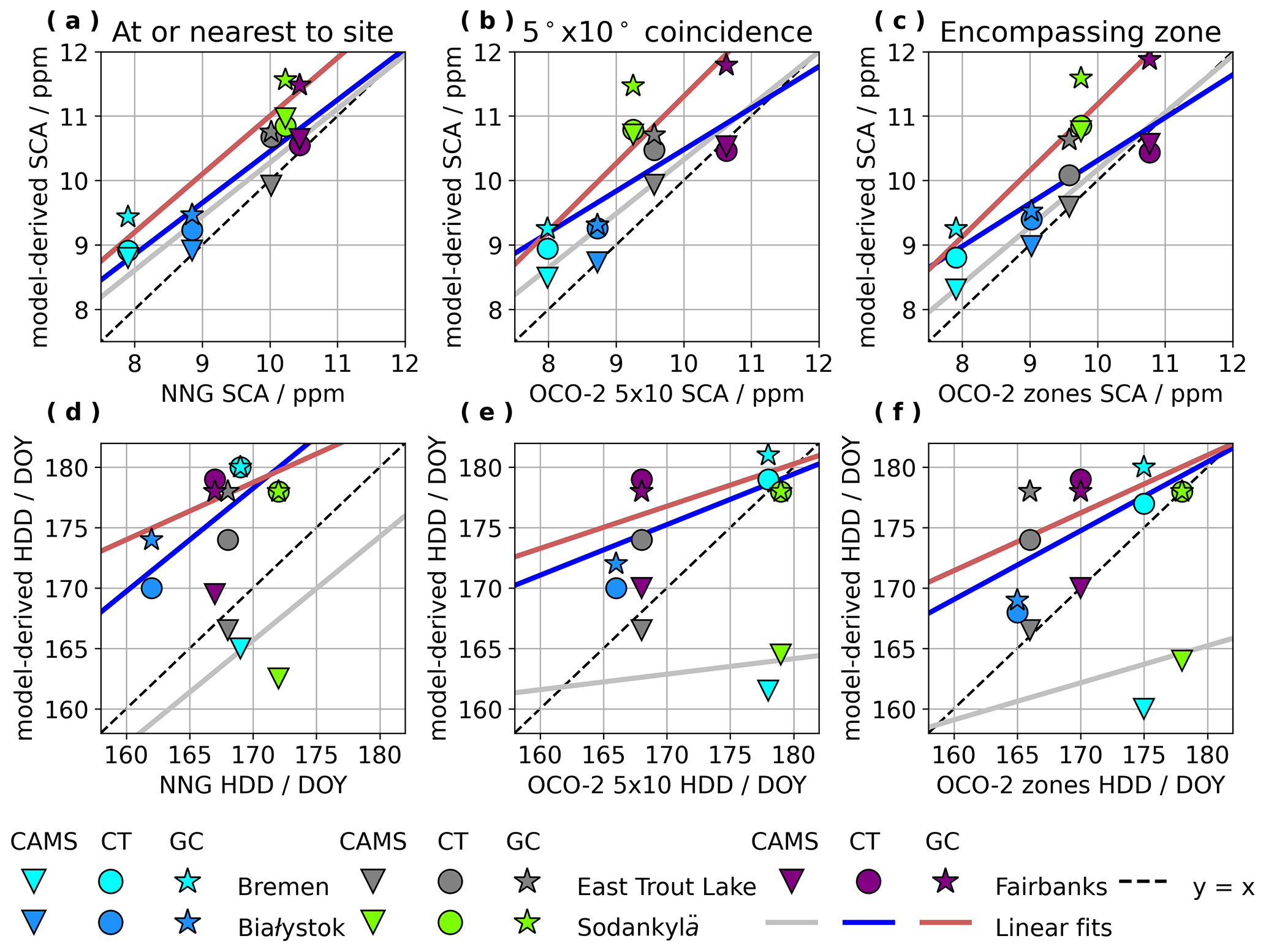
Figure 2 Correlations of observed versus model-derived SCA and HDD. Observed $X_{{\mathrm{CO}}_{\mathrm{2}}}$ seasonal cycles are based on NNG and OCO-2 satellite-based observations, while model-derived $X_{{\mathrm{CO}}_{\mathrm{2}}}$ seasonal cycles are based on estimates from the CAMS, CT2019B, and GC-CT2019 model frameworks. SCA and HDD are compared for three spatial types at each of the five ground sites: seasonal fits of near-noon ground-based (NNG) observations from TCCON and EM27/SUN measurements are compared to fits of daily model estimates at the nearest model grid point to the ground site; seasonal fits of daily average OCO-2 retrievals that fall within the 5^∘ latitude by 10^∘ longitude region of coincidence, centered on the location of each ground site, are compared to fits of daily model estimates averaged across the coincidence region; seasonal fits of OCO-2 daily averages for the 5^∘ latitude by 20^∘ longitude zone containing each ground site are compared to fits of daily model estimates averaged across those same zones (see map in Fig. 1 and site details in Table 1).

3 Results

3.1 $X_{{\mathrm{CO}}_{\mathrm{2}}}$ seasonal cycles near ground sites

Before attempting to interpret spatial distributions of seasonal cycle parameters on continental scales, it is of value to get a better idea of how seasonal cycle parameters from observations at a single location compare to those from spatially averaged data. To this end, five high-latitude sites are considered with long-term ground-based observations, as described in Sect. 2.2. There are three spatial scales considered with seasonal cycle fits to near-noon ground-based (NNG) observations and seasonal cycle fits to spatially averaged data over a commonly used satellite coincidence region of 5^∘ latitude by 10^∘ longitude centered on the location of the ground site, as well as over the 5^∘ latitude by 20^∘ longitude zone in which the ground site is located (reference zones in Fig. 1). In Fig. 2, observed SCAs and HDDs from NNG and OCO-2 observations are correlated against model-derived SCAs and HDDs from CAMS, CT2019B, and GC-CT2019 at each of the three spatial scales, and the corresponding linear regression equations and correlation coefficients are reported in Table 2. These correlations exhibit tight linearity for SCA (with most R²>0.7) and reasonable linearity for HDD when comparing observed and model-derived parameters at all scales. SCAs from CAMS or CT2019B are in better agreement with observations than those from GC-CT2019 in every case, as demonstrated by the fact that the CAMS and CT2019B linear regressions fall closer to the y=x line than the GC-CT2019 linear regression in panels (a), (b), and (c) of Fig. 2. Agreement between model-derived and observed HDD is better for the single-point model estimates nearest the ground site versus NNG results in panel (d) of Fig. 2, and the scatter increases in the comparisons of HDD from spatially averaged model estimates versus spatially averaged OCO-2 observations in panels (e) and (f) of Fig. 2. All three models tend to yield slightly larger SCAs than observations at all sites, as well as later HDD than observations with the exception of CAMS HDD at Bremen and Sodankylä. These results stand in contrast to earlier work by Yang et al. (2007), who found that the Transcom model underestimated SCA of CO₂ mixing ratios relative to aircraft observations at nearly every altitude. Details of the full time series, plots of seasonal cycle fits, and seasonal cycle fit parameters, with uncertainties, for these ground sites, coincidence regions, and encompassing zones are reported in the Supplement.

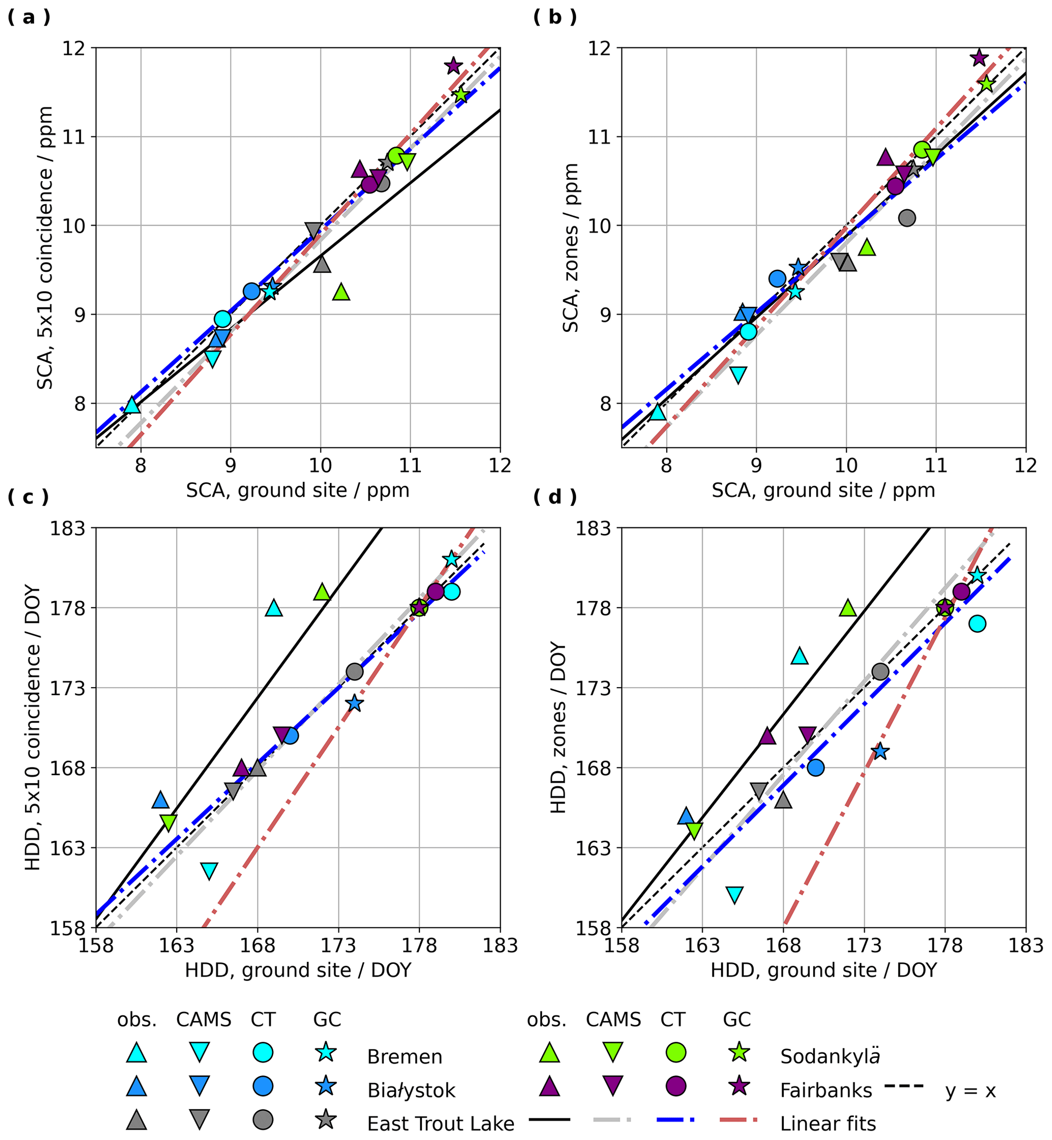
Figure 3 Correlations of SCA and HDD from NNG observations or the model grid point nearest the ground site versus SCA and HDD from spatially averaged OCO-2 observations or model estimates. For these correlations, we only compare across spatial scales by pairing NNG observations with spatially averaged OCO-2 data and pairing single-point CAMS, CT2019B, and GC-CT2019 model estimates nearest to the ground sites with corresponding spatially averaged model estimates in the same model framework. Note that there are some overlapping points in the correlations of HDD in panels (c) and (d) that may visually obscure some of the results.

In Fig. 3 and Table 3 the relationships between seasonal cycle parameters from spatially averaged data versus those from a single point, at or nearest the ground sites, are explored. In this case, seasonal cycle parameters derived from NNG observations are correlated against seasonal cycle parameters derived from spatially averaged OCO-2 retrievals, while model-derived seasonal cycle parameters for a single point near the ground site are correlated against model-derived seasonal cycle parameters from spatially averaged model estimates. Jacobs et al. (2020) have shown that an alternative bias correction, parameterized for temperature at 700 hPa, resulted in reduced seasonality in OCO-2 bias within the 5^∘ latitude by 10^∘ longitude coincidence region relative to NNG observations at East Trout Lake, Sodankylä, and Fairbanks. Results in the Supplement show that the alternative bias correction improved agreement in both SCA and HDD between NNG seasonal cycles and coincident OCO-2 seasonal cycles. The results in Fig. 3 and Table 3 indicate that HDD correlations across scales tend to be slightly weaker and markedly different depending on whether one considers observed or model-derived seasonal cycles. For the coincidence region and the encompassing zone, OCO-2 data consistently yield later HDD than NNG data, while spatially averaged model estimates tend to yield HDD that is in good agreement or slightly earlier than the point nearest to the ground site. SCAs for ground sites are well correlated and mostly in close agreement with both SCAs for 5^∘ latitude by 10^∘ longitude coincidence regions and SCAs for encompassing 5^∘ latitude by 20^∘ longitude zones, demonstrating that SCA scales well with spatial averaging and is a credible metric to consider in the context of this analysis. The relatively weaker correlations in HDD across spatial scales in panels (c) and (d) of Fig. 3 suggest greater spatial heterogeneity in HDD within zones from both observed and model-derived seasonal cycles. This result, in combination with the scatter in panels (d), (e), and (f) of Fig. 2, implies that HDD may display more random variability than SCA and may therefore be a less useful metric in this context.

Table 2 Linear regression equations and correlation coefficients for the correlations, presented in Fig. 2, of model-derived versus observed SCA and HDD at three spatial scales for five ground sites.

Table 3 Linear regression equations and correlation coefficients for the correlations in Fig. 3 in which SCA and HDD from NNG or model estimates near the ground sites are compared to SCA and HDD from spatially averaged satellite observations or spatially averaged model estimates over the corresponding 5^∘ latitude by 10^∘ longitude coincidence regions and encompassing 5^∘ latitude by 20^∘ longitude zones.

3.2 $X_{{\mathrm{CO}}_{\mathrm{2}}}$ seasonal cycles by zone

The full set of seasonal cycle fit parameters, corresponding uncertainty estimates, and plots of time series and seasonal cycle fits for each zone and ground site in Fig. 1 are reported in the Supplement. While the fits to model estimates are generally similar in shape with fits to observations, there are some zones that yield an unrealistic drop in wintertime values in the OCO-2 seasonal cycle fits, which is more pronounced for zones with fewer satellite-based $X_{{\mathrm{CO}}_{\mathrm{2}}}$ observations near the peak and trough of the seasonal cycle. This wintertime drop in the shape of the seasonal cycle is evidence that should motivate further efforts to increase satellite-based observations over high-latitude regions outside of the summer months. Only a small number of zones, particularly in the Asian tundra, have seasonal cycle fits that are obviously compromised by insufficient data in spring and autumn, while the majority of zones have seasonal fits that look reasonable and are similar to seasonal cycle fits to continuous model estimates, with the exception of the noted wintertime drop. An analysis of changes in CAMS seasonal cycle fits when selecting only days with OCO-2 observations available rather than the full continuous time series of model estimates is presented in the Supplement, which indicates that shifts in CAMS SCA due to imposed data gaps are $-\mathrm{0.044}\pm \mathrm{0.197}$ ppm, with shifts in SCA for all zones less than 0.5 ppm, while biases in CAMS SCA for the full time series relative to OCO-2 SCA are 0.547±0.720 ppm and range from −1.0 to 3.0 ppm. These shifts in CAMS SCA are also small relative to the approximately 5 ppm variability in SCA seen across the northern high-latitude regions. In addition, the Lindqvist method of fitting (Lindqvist et al., 2015) still provides a more constrained shape than a fit to a truncated Fourier series, which can yield highly unrealistic oscillations in time series with only minimal gaps in data coverage. The close similarities between spatial distributions of seasonal cycle parameters from OCO-2, CAMS, CT2019B, and GC-CT2019 are apparent in Fig. 4.

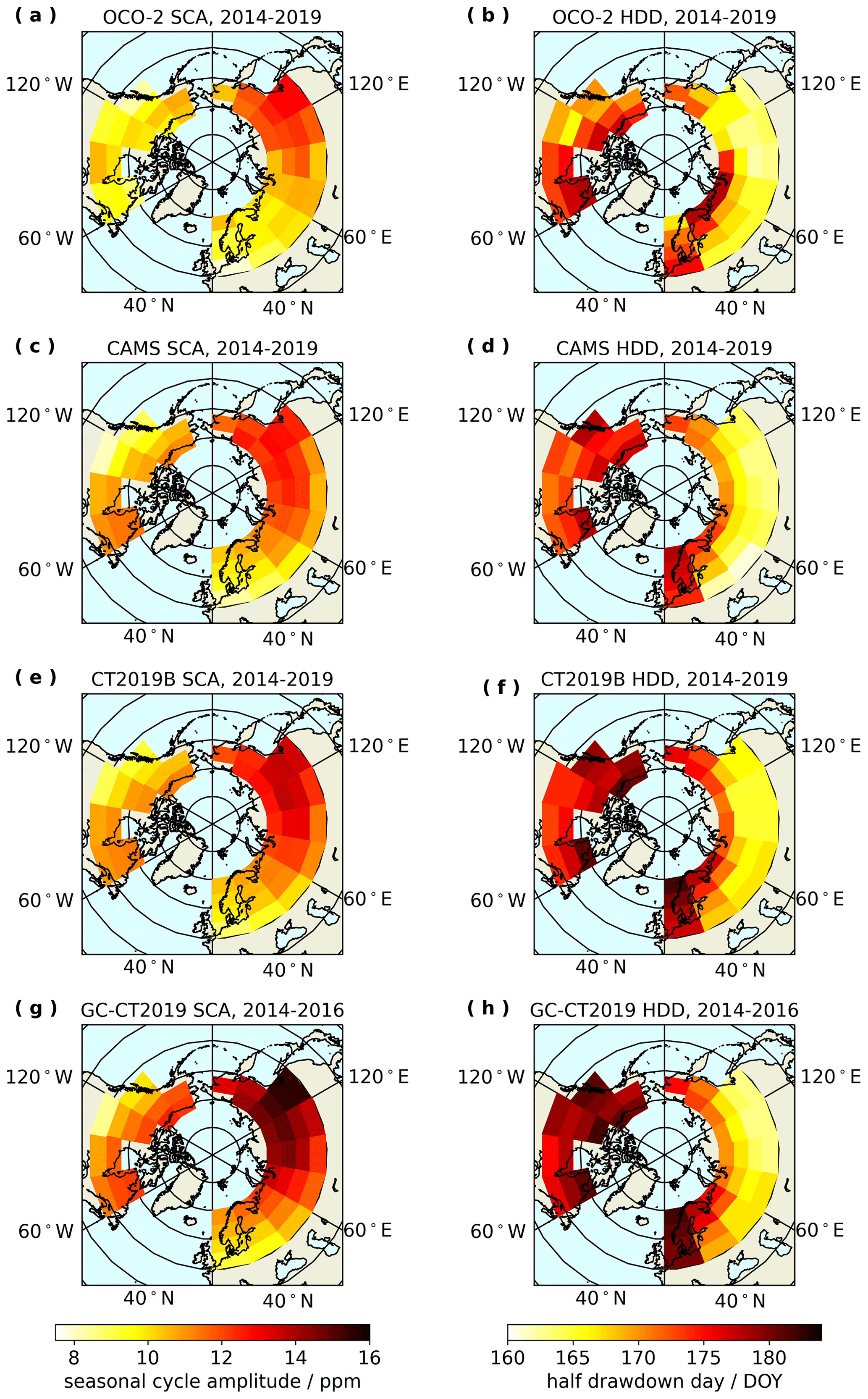
Figure 4 Maps of SCA and HDD (represented as color scaling) from seasonal cycle fits to OCO-2 observations and model estimates from CAMS, CT2019B, and GC-CT2019 for each zone defined in Fig. 1.

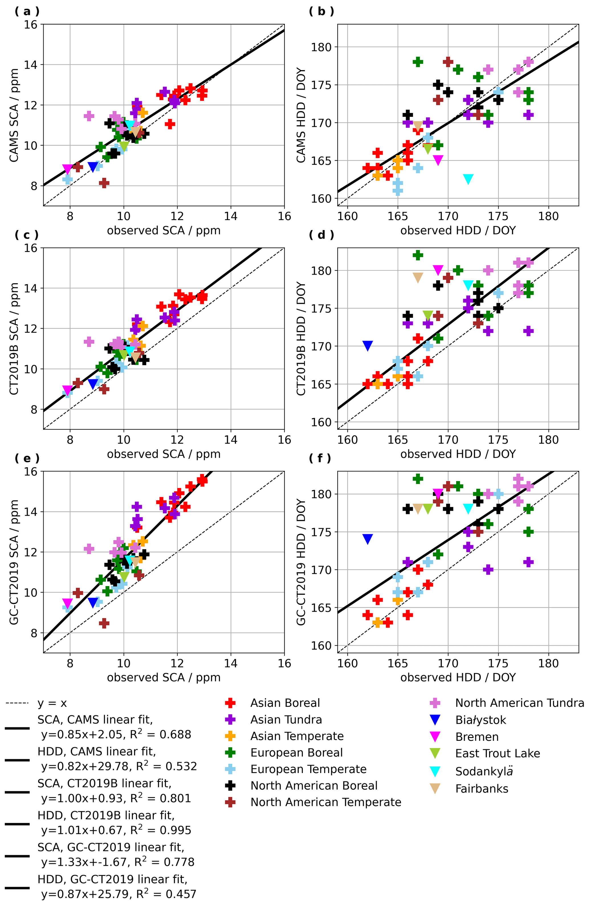
Figure 5 Plots of model-derived versus observed SCA and HDD using the model estimated from CAMS (a, b), CT2019B (c, d), and GC-CT2019 (e, f), and using observations from OCO-2 within 5^∘ latitude by 20^∘ longitude zones and NNG observations at five ground sites.

Comparing observed and model-derived SCA and HDD

Direct correlations of model-derived versus observed SCA and HDD are shown in Fig. 5, indicating that model-derived and observed SCAs agree with tight linearity (R²>0.68) while model-derived and observed HDD agree with reasonable linearity (R²>0.45). Model estimates tend to yield slightly larger SCA and later HDD than OCO-2 and NNG observations. The most notable discrepancies between observed and model-derived SCAs tend to occur in the Asian tundra and North American tundra regions for which model estimates yield larger values of SCA that are more homogeneous across zones than observations. SCAs and HDDs from CAMS and CT2019B model-derived seasonal cycles are in better agreement with observed SCA and HDD than those from GC-CT2019. For SCA in particular, the CAMS and CT2019B seasonal cycles are in very close agreement with OCO-2 seasonal cycles when satellite retrievals are treated with the alternative high-latitude quality controls and bias correction described by Jacobs et al. (2020) (see Sects. 2.1 and S2). SCAs and HDDs derived from GC-CT2019 (see panels e and f of Fig. 5) cover a broader range of values, particularly overestimating SCA in the Asian boreal and tundra regions and exhibiting more scatter in correlations of model-derived versus observed HDD. GC-CT2019 SCAs remain strongly correlated with observed SCAs, but the slope of this correlation is steeper than for CAMS and CT2019B model estimates.

3.3 Spatial distributions of SCA and HDD

Seasonal cycle amplitudes (SCA) and half drawdown day (HDD) are mapped in Fig. 4, showing results from OCO-2 observations, CAMS model estimates, CT2019B model estimates, and GC-CT2019 model estimates of $X_{{\mathrm{CO}}_{\mathrm{2}}}$. Figure 4 demonstrates that both OCO-2 observations and model estimates from CAMS, CT2019B, and GC-CT2019 yield larger SCAs and earlier HDDs in the Asian boreal forest than any other region. The earlier seasonal timing of the Asian boreal forest zones is consistent with results from Keppel-Aleks et al. (2012) and Schneising et al. (2011), and these studies also linked earlier drawdown in Asia to larger SCA. Although one would not necessarily expect SCA of surface in situ measurements to match SCA of $X_{{\mathrm{CO}}_{\mathrm{2}}}$, this finding also aligns with the study by Lin et al. (2020), who found that Siberia had the largest SCA in surface CO₂ concentrations when normalized for area. The CAMS, CT2019B, and GC-CT2019 results in Fig. 4 exhibit more apparent latitudinal gradients, whereas the results from OCO-2 show more spatial heterogeneity, and this is particularly true for HDD. Seasonal cycles of direct observations are expected to display more heterogeneity than seasonal cycles of model estimates, which depend on mathematical modeling of atmospheric transport to calculate $X_{{\mathrm{CO}}_{\mathrm{2}}}$, even if the underlying fluxes are based on in situ data assimilation. Overall, the spatial distributions in SCA and HDD from OCO-2 agree more with those from CAMS and CT2019B than those from GC-CT2019. GC-CT2019 yields larger magnitudes of SCA for many regions, as well as SCAs and HDDs spread across a larger range for northern high-latitude regions, relative to SCAs from OCO-2, CAMS, or CT2019B. In addition, OCO-2 observations yield notably smaller SCA than CAMS, CT2019B, or GC-CT2019 in the western zones of the Asian boreal forest, in the Asian tundra, and in the eastern zones of North America.

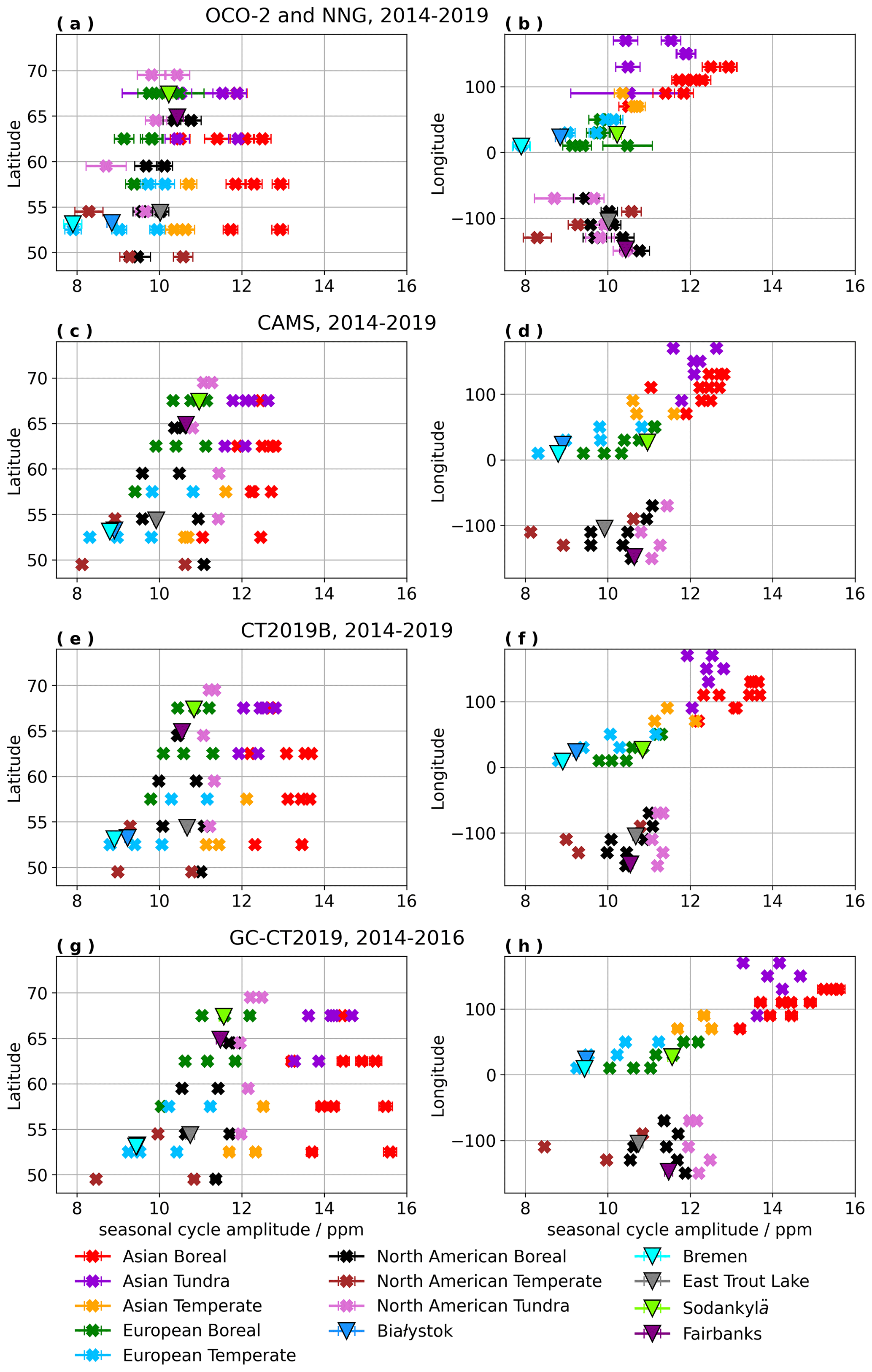
Figure 6 Plots of latitude and longitude correlated to SCA using observational results from OCO-2 and NNG observations (a, b), CAMS model estimates (c, d), CT2019B model estimates (e, f), and GC-CT2019 model estimates (g, h). The latitude and longitude for each zone is located at its center.

Panels (a), (c), (e), and (g) of Fig. 6 show a clear increase in SCA from west to east across the Eurasian continent in both model-derived and observational results. In North America, longitudinal gradients are more subtle. While OCO-2 observations exhibit a slight gradient in SCA across North America that increases from east to west, CAMS, CT2019, and GC-CT2019 yield SCAs that increase from west to east, in the same direction as gradients across Eurasia. This discrepancy in North America hinges primarily on the zones of boreal forest and tundra in eastern North America, which have the smallest SCAs for that continent when using OCO-2 data but have the largest SCAs for that continent when using CAMS, CT2019B, or GC-CT2019 model estimates. As expected, panels (a), (c), (e), and (g) in Fig. 6 show latitudinal gradients with increasing SCA from south to north for both observed and model-derived seasonal cycles. However, the Asian boreal forest zones stand apart from other regions in all panels of Fig. 6, particularly when plotted against latitude, with larger SCA than other data at similar latitudes or longitudes. Results in Fig. 7 demonstrate that HDDs are far more scattered and do not follow the distinct trends with latitude and longitude that SCAs do. HDD spatial gradients seem to be inverted relative to SCA with a vague tendency toward later HDD at more northern latitudes and more western longitudes, and HDD also exhibits similar discrepancies between observed and model-derived longitudinal gradients for North America.

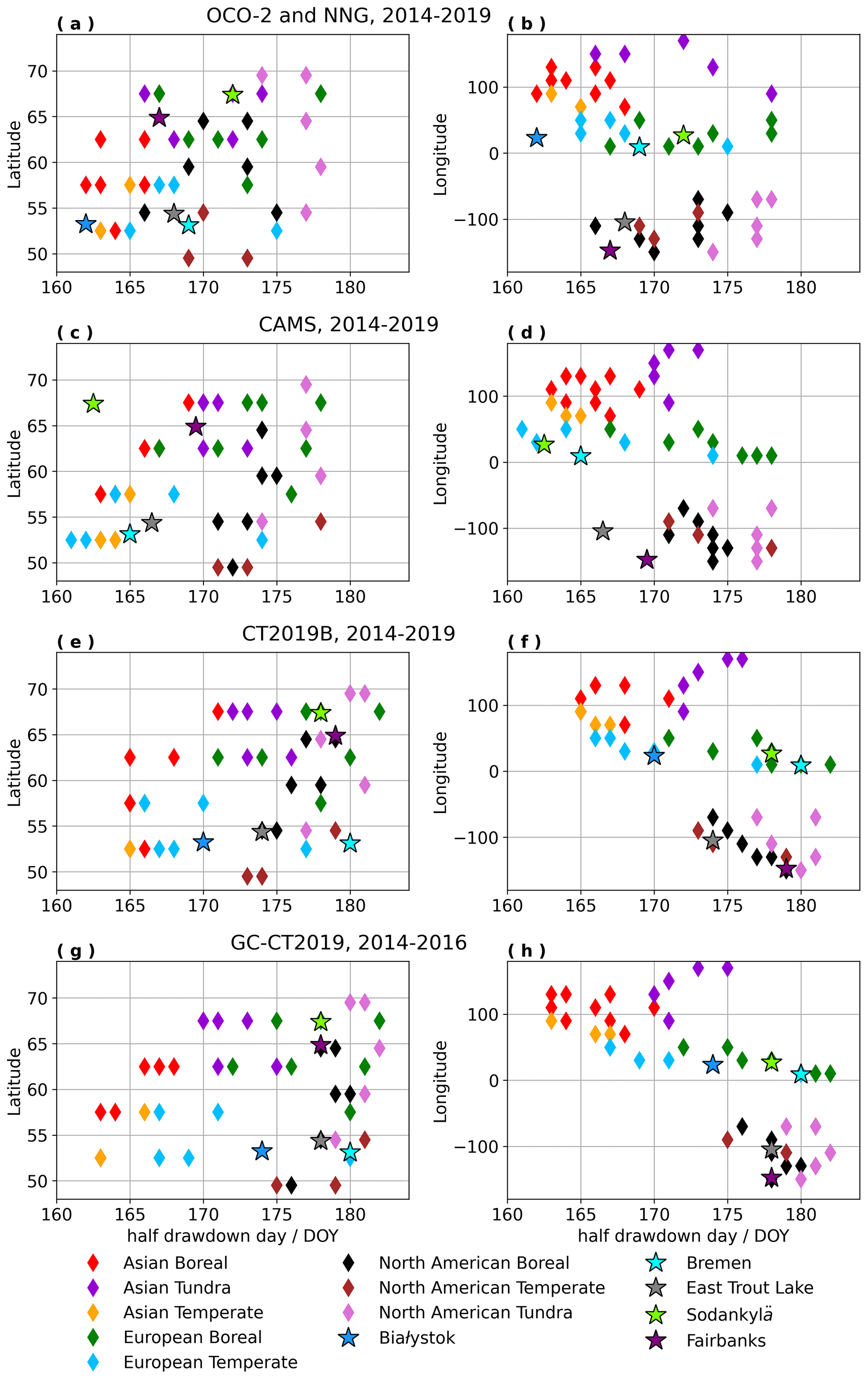
Figure 7 Plots of latitude and longitude correlated to HDD using observational results from OCO-2 and NNG observations (a, b), CAMS model estimates (c, d), CT2019B model estimates (e, f), and GC-CT2019 model estimates (g, h). The latitude and longitude for each zone is located at its center.

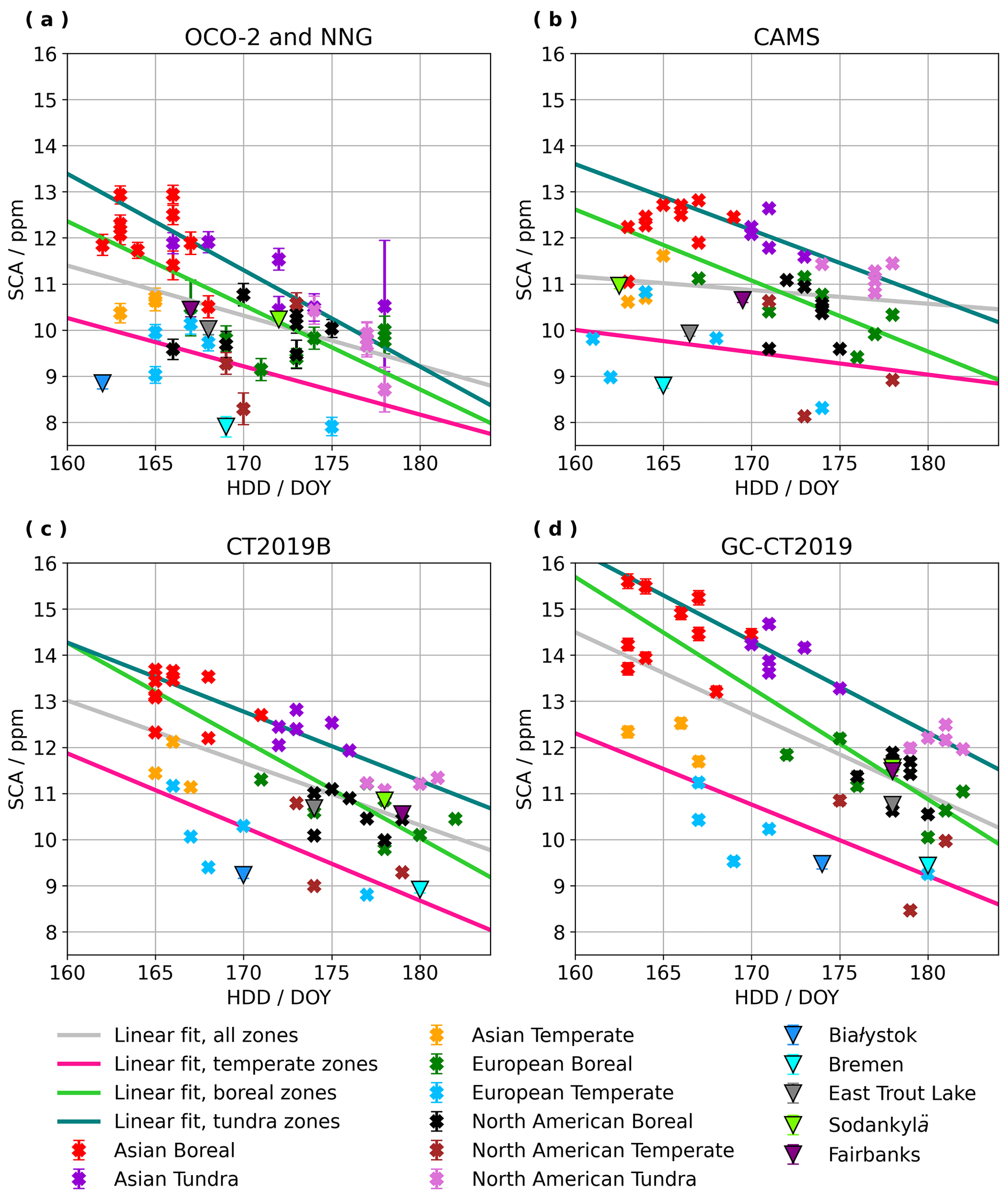
Figure 8 Correlations between SCA and HDD using OCO-2 and NNG seasonal cycle fits (a), CAMS seasonal cycle fits (b), CT2019B seasonal cycle fits (c), and GC-CT2019 seasonal cycle fits (d). Linear regressions are plotted for all zones, as well as separately for temperate, boreal, and tundra regions.

3.4 The relationship between SCA and HDD

Figure 8 and the calculated linear regressions in Table 4 show that there is a negative correlation between HDD and SCA for both observed and model-derived seasonal cycle fits, such that earlier HDD corresponds to larger SCA. CAMS model estimates yield correlations between HDD and SCA that are more similar to those from OCO-2 and NNG measurements, while GC-CT2019 yields stronger correlations with steeper slopes. The results in Fig. 8 emphasize the exceptionally early HDD and large SCA of the Asian boreal forest, such that many of the Asian boreal zones fall more in line with the tundra zones than with the other boreal zones. A latitudinal gradient is suggested by the fact that the linear regressions plotted in Fig. 8 are shifted up for the tundra zones and shifted down for the temperate zones, with the boreal zones in between the two. Furthermore, the separate linear regressions for the temperate, boreal, and tundra zones plotted in Fig. 8 have much larger R² than the linear regressions for all the zones together (see Table 4), suggesting that there are different dynamics in different biomes that affect relationships between extent and timing of apparent CO₂ uptake. The strength of this correlation in observed and CAMS seasonal cycles was highest for tundra and lowest for temperate zones with the boreal zones falling in between.

Table 4 Linear regression equations and correlation coefficients for the correlations in Fig. 8 in which SCA is correlated against HDD for observed and model-derived results. Linear regressions were calculated considering all 5^∘ latitude by 20^∘ longitude zones and then separately for zones in temperate, boreal, and tundra regions.

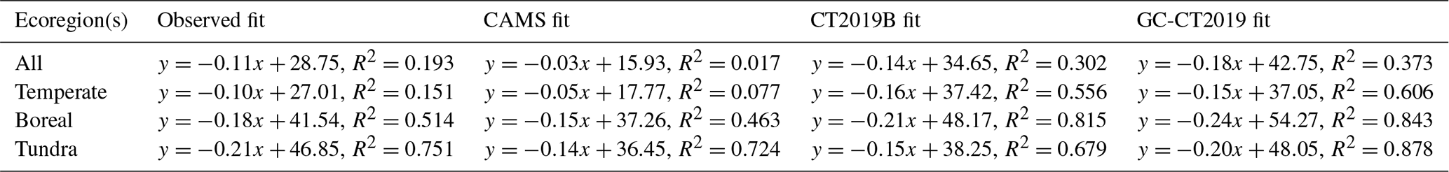
Figure 9 Maps of GEOS-Chem surface contact tracer contributions from land and ocean with 5, 15, 30, and 90 d lifetimes for each zone, with units that are scaled relative to an arbitrary initial release of tracer particles. Surface contact tracer contributions shown here are calculated as an average of all days in the simulation period, 2014–2016.

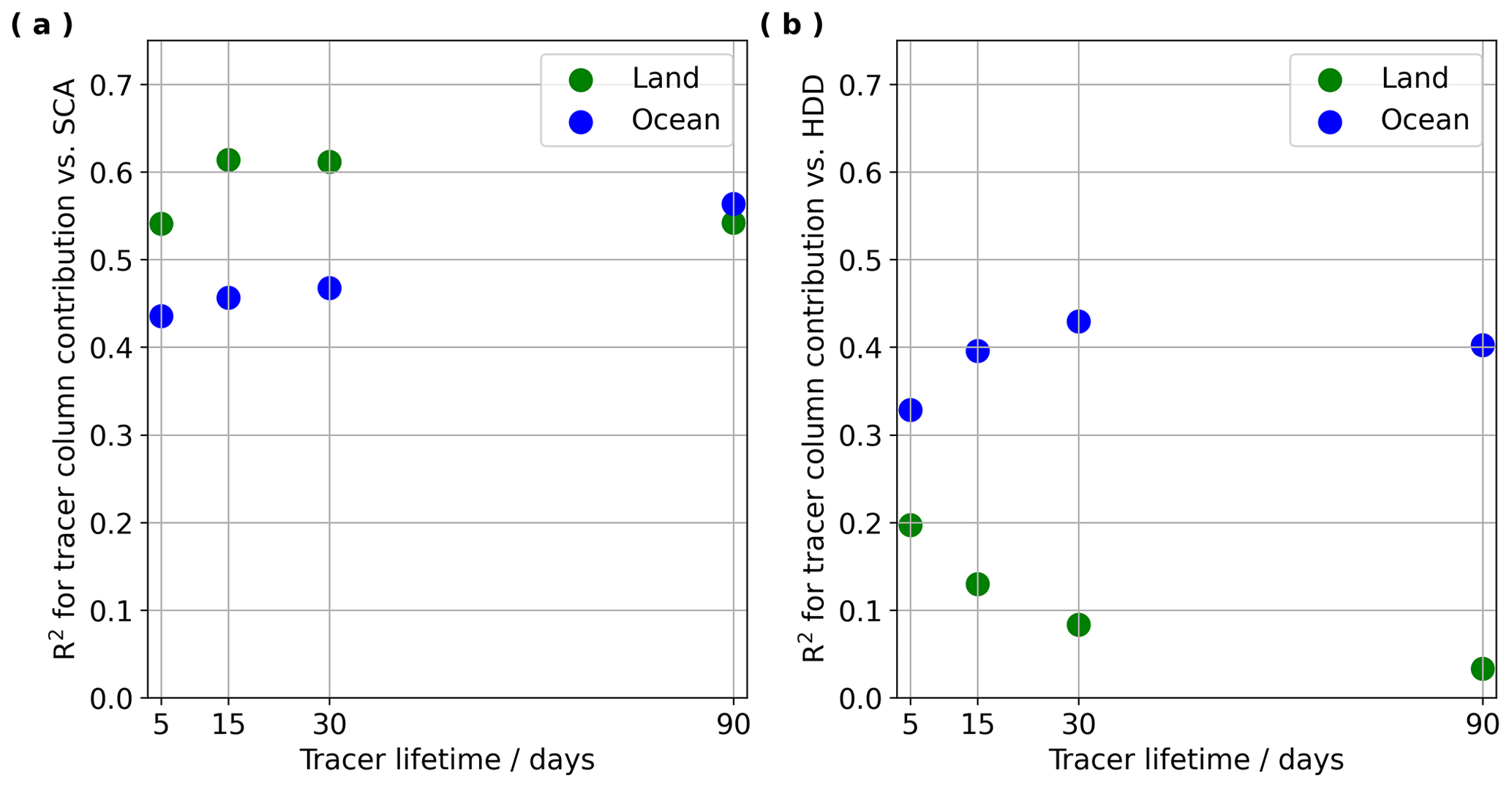
Figure 10 Panel (a) shows correlation coefficients for surface contact tracer contributions from land and ocean (mapped in Fig. 9) versus OCO-2 SCA (mapped in Fig. 4a), and panel (b) shows correlation coefficients for surface contact tracer contributions from land and ocean versus OCO-2 HDD (mapped in Fig. 4b).

3.5 Comparing GEOS-Chem surface contact tracers to observed SCA and HDD

GEOS-Chem surface contact tracers were used to simulate the release of tracers from land and ocean yielding relative concentrations of tracers with lifetimes of 5, 15, 30, and 90 d for a given grid point and day. In these results the relative contributions of surface contact tracers for each zone represent an overall average of surface contact tracer contributions for all days in 2014–2016 and aggregated spatially across the 5^∘ latitude by 20^∘ longitude zone. The surface contact tracers show that the largest $X_{{\mathrm{CO}}_{\mathrm{2}}}$ SCAs occur in areas with the greatest influence from air that contacted land surfaces 15 to 30 d prior. There are clear similarities in the spatial distributions of SCA in panels (a), (c), and (e) of Fig. 4 and those of the surface contact tracers from land with a 15 or 30 d lifetime, as shown in panels (c) and (e) of Fig. 9. There are also similarities in the spatial distributions of HDD in panels (b), (d), and (f) of Fig. 4 and those for the surface contact tracers from ocean with a 15 or 30 d lifetime, as shown in panels (d) and (f) of Fig. 9. The relative strength of linear relationships between seasonal cycle parameters from OCO-2 observations and surface contact tracers is quantified with correlation coefficients in Fig. 10. Figure 10 shows that the observed SCAs are most correlated with land-based surface contact tracers with 15 and 30 d atmospheric lifetimes, while observed HDDs are most correlated with ocean-based surface contact tracers with 15 and 30 d atmospheric lifetimes. Correlations between HDD and land tracers are weak (see Fig. S45) and seem to follow a curve rather than a line or may be representative of two different linear relationships for different groups of zones. The correlations with ocean tracers were always inverted relative to those with land tracers, such that reduced contribution from ocean tracers and increased contributions from land tracers consistently correspond with larger SCA and often correspond with earlier HDD.

4 Discussion

In this analysis, methods described by Lindqvist et al. (2015) were used to fit daily average time series of daily $X_{{\mathrm{CO}}_{\mathrm{2}}}$ to a skewed sine wave (see Eq. 1) and subsequently calculate seasonal cycle amplitude (SCA) and half drawdown day (HDD), as described in Sect. 2.4. These fitting methods have been found to yield more stable and realistic fits for time series with winter gaps than fitting to a truncated Fourier series. Increased OCO-2 throughput (Kiel et al., 2019; O'Dell et al., 2018; Osterman et al., 2018) and use of a bias correction and quality control methods tailored to northern high latitudes (Jacobs et al., 2020) improve the availability of OCO-2 data at the edges of the growing season and assist in generating stable and realistic seasonal cycle fits. Results in Fig. 3 and Table 3 indicate close agreement between SCAs from NNG observations at five ground sites and corresponding SCAs from OCO-2 data in the 5^∘ latitude by 10^∘ longitude spatial coincidence regions. Relatively weak correlations in HDD at the five ground sites, both across spatial scales and between observed and model-derived seasonal cycles, are likely to be at least partly attributable to spatial heterogeneity in seasonal cycle timing within 5^∘ latitude by 20^∘ longitude zones. It is possible that HDD as a phase metric is not as well constrained by the seasonal cycle fitting methods used here as SCA. Many of the greatest discrepancies in HDD when comparing coincidence regions or zones to ground sites (see Fig. 3 and Table 3) occur in observed seasonal cycles and may arise from disagreement between NNG and OCO-2 observations. Discrepancies between observed and model-derived HDD, which are most apparent for GC-CT2019 $X_{{\mathrm{CO}}_{\mathrm{2}}}$ estimates, could reflect an inaccurate representation of ecosystem respiration in the CASA terrestrial biosphere model, which underlies the CarbonTracker2019 biospheric fluxes used in the GC-CT2019. Byrne et al. (2018) found that differences in the seasonal timing of net ecosystem exchange (NEE) maximum drawdown were primarily driven by differences in the timing of ecosystem respiration in spring and fall, while the amplitude of NEE was largely influenced by the magnitude of peak gross primary production (GPP). This could explain the higher degree of spatial heterogeneity in seasonal cycle timing because ecosystem respiration is driven by soil temperature, soil moisture, and litter accumulation, which could all be expected to exhibit a higher degree of spatial heterogeneity than ambient temperature and sunlight,. If there is, in truth, more spatial heterogeneity in the timing of seasonal CO₂ uptake, then a failure to accurately represent these spatial distributions in timing could be exacerbated by errors or differences in atmospheric transport modeling and result in larger or more variable discrepancies between observed and model-derived HDD. In this case, the relatively spatially homogeneous values of SCA would be easier to accurately predict in the models than HDD. Alternatively, if SCA is primarily defined by the magnitude of maximum GPP, it may be better constrained in the models because data products like solar-induced fluorescence (SIF) and the normalized difference vegetation index (NDVI) can be used to validate model estimates of GPP, while ecosystem respiration does not have a direct data proxy.

OCO-2, CAMS, CT2019B, and GC-CT2019 all yield very similar spatial distributions of SCA and HDD across the northern high-latitude regions (see map in Fig. 1), and both had large SCA and early HDD in the Asian boreal forest as well as a clear increase in SCA from west to east across the Eurasian continent. We found an inverse linear relationship between SCA and HDD across northern high latitudes for both observed and model-derived seasonal cycle fits (see Fig. 8 and Table 4), and these correlations were stronger when separating by ecological type (temperate, boreal, or tundra). This relationship is an interesting result of this analysis that warrants a more in depth exploration in future work, though we cannot speculate on the cause of this phenomenon in the context of this study. Discrepancies between SCA from GC-CT2019 and SCAs from CAMS, CT2019B, and observations are consistent with the assessments of seasonal bias resulting from the GEOS-Chem transport modeling framework with MERRA-2 meteorology, as described by Schuh et al. (2019), but may also be partly explained by the lack of internally consistent atmospheric transport modeling for CO₂ flux and $X_{{\mathrm{CO}}_{\mathrm{2}}}$ estimates in the GC-CT2019 framework. Schuh et al. (2019) found that the GEOS-Chem CO₂ simulation overestimates $X_{{\mathrm{CO}}_{\mathrm{2}}}$ in winter and underestimates $X_{{\mathrm{CO}}_{\mathrm{2}}}$ in summer relative to the TM5 transport model, yielding an exaggerated seasonal oscillation and larger SCA. Byrne et al. (2018) found that CarbonTracker2016, using CASA to constrain biospheric carbon exchange, estimated later NEE drawdown than flux inversions with either GOSAT or TCCON data assimilation, and this appears to be consistent with the later HDD estimated by the GC-CT2019. Despite these discrepancies, we contend that the strong correlations between GC-CT2019 and observational results (see panels e and f for Fig. 5) suggest that GEOS-Chem simulations remain a useful tool for investigating the broader implications of spatial distributions in SCA and HDD from OCO-2 observations.

Two limiting hypotheses for the origin of the spatial patterns in $X_{{\mathrm{CO}}_{\mathrm{2}}}$ SCA shown in Fig. 4 are that they arise from differences in flux magnitudes within the 5^∘ latitude by 20^∘ longitude zone or that they arise from transport patterns accumulating CO₂ exchanges across multiple zones or regions. To investigate the relative influences of atmospheric transport or fluxes within zones on $X_{{\mathrm{CO}}_{\mathrm{2}}}$ seasonal cycles, we consider source apportionment from the GEOS-Chem CO₂ simulation (Nassar et al., 2010) and GEOS-Chem surface contact tracers, as well as surface CO₂ flux estimates from CarbonTracker2019 and CAMS models.

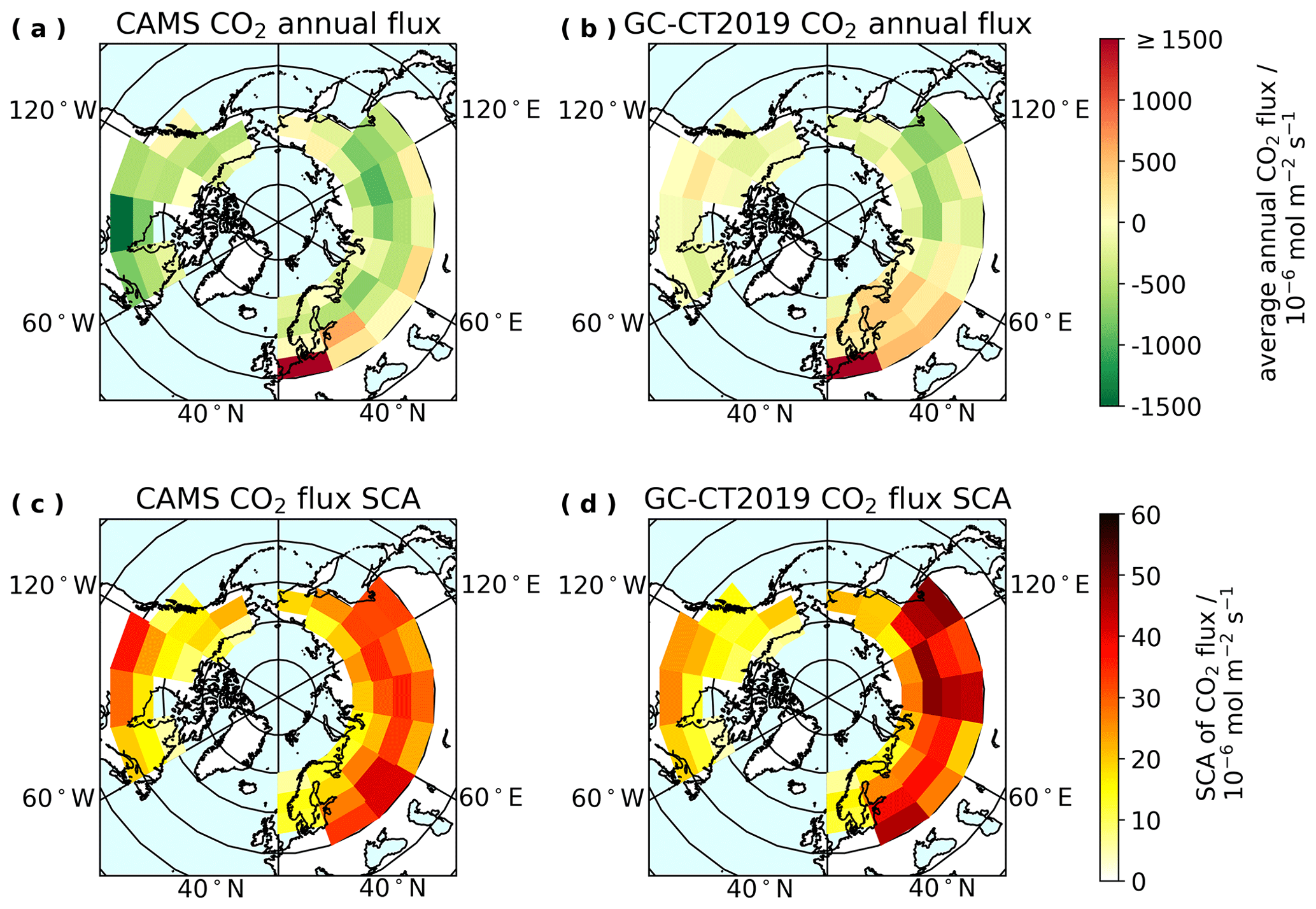
Figure 11 Maps of average total annual CO₂ flux, using GC-CT2019 (GC) and CAMS flux estimates (a, b), and SCA in CO₂ flux, calculated as the difference between the maximum and minimum of the average annual cycle in flux (c, d).

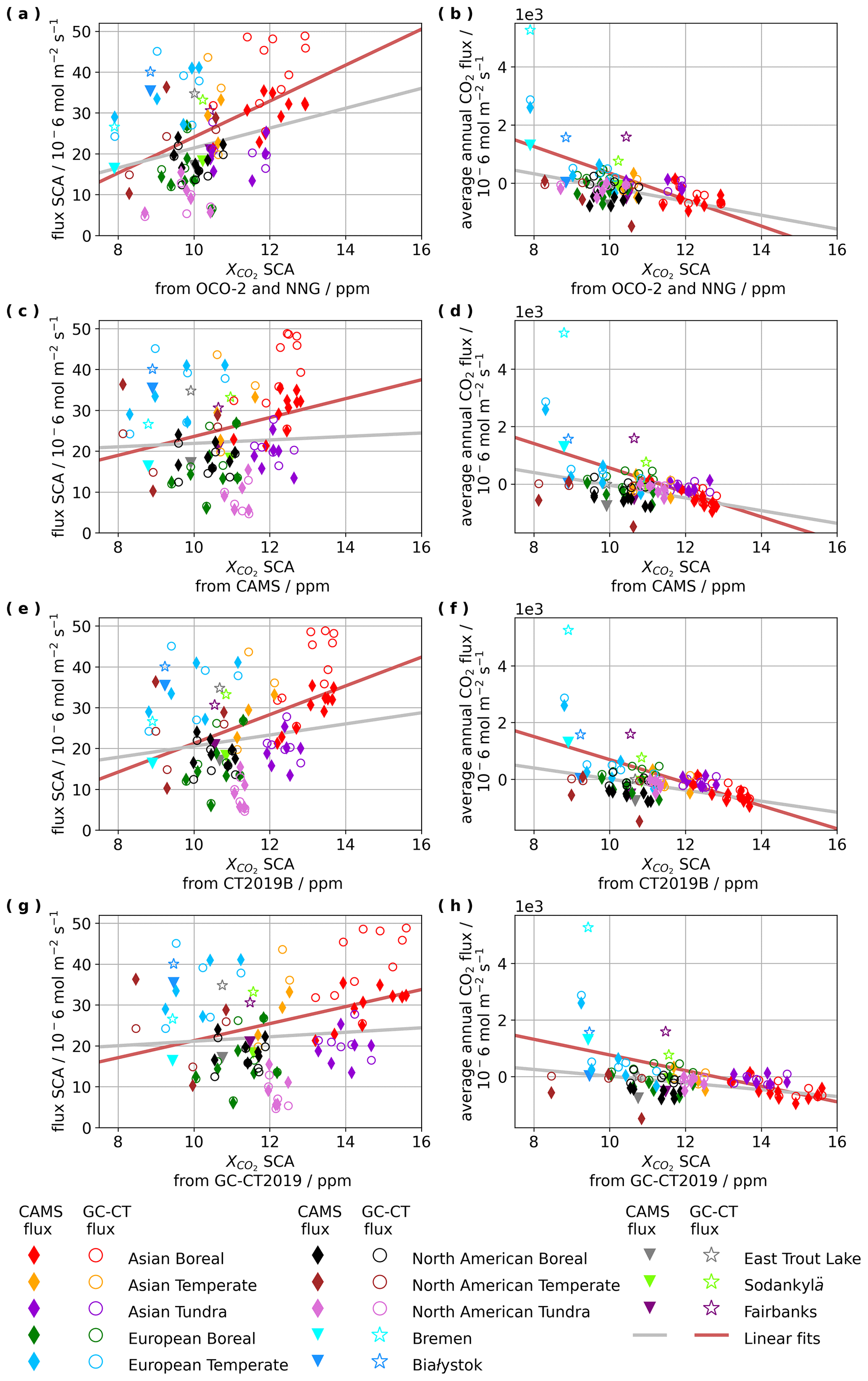
Figure 12 Correlation plots of flux SCA and average annual fluxes from CAMS and GC-CT2019 versus $X_{{\mathrm{CO}}_{\mathrm{2}}}$ SCA from OCO-2 and NNG, as well as model-derived $X_{{\mathrm{CO}}_{\mathrm{2}}}$ SCA from CAMS, CT2019B, and GC-CT2019.

Figure 13 Correlation coefficients for the linear fits in Fig. 12, as well as alternative correlation coefficients for average annual fluxes versus $X_{{\mathrm{CO}}_{\mathrm{2}}}$ SCA with European temperate zone 3 and Bremen removed.

4.1 The role of atmospheric transport in shaping $X_{{\mathrm{CO}}_{\mathrm{2}}}$ seasonality

Fisher et al. (2010) and Wang et al. (2011) demonstrated the ability of GEOS-Chem to represent synoptic transport from midlatitudes to the Arctic. Schuh et al. (2019) evaluated meridional transport of CO₂ and SF₆ in GEOS-Chem, using the same MERRA-2 meteorology used here, and suggested that the model may underestimate vertical and meridional mixing, which slightly increases CO₂ seasonal cycle amplitude in GEOS-Chem in high northern latitudes compared to some other models. Despite some discrepancies in SCA and HDD from GC-CT2019, relative to observed SCA and HDD, which may arise from differences between the GEOS-Chem and TM5 atmospheric transport models, the GEOS-Chem transport model reproduces surface temperature and pressure patterns and thus is a reasonable representation of atmospheric transport (Wang et al., 2011; Fisher et al., 2010). Therefore, comparing these GEOS-Chem surface contact tracers with observed SCA and HDD should provide useful insights into the influence of atmospheric transport patterns on observed $X_{{\mathrm{CO}}_{\mathrm{2}}}$ seasonality. The higher correlation coefficients obtained when comparing OCO-2 SCAs to land and ocean tracers with 15 and 30 d lifetimes suggest that accumulation of CO₂ flux due to atmospheric transport on roughly monthly timescales plays an important role in affecting $X_{{\mathrm{CO}}_{\mathrm{2}}}$ SCA.

4.2 The role of CO₂ fluxes in $X_{{\mathrm{CO}}_{\mathrm{2}}}$ SCA

Figure 11 shows maps of average annual fluxes and flux SCAs for GC-CT2019 and CAMS, which show that flux SCAs in panels (c) and (d) are distributed without the apparent longitudinal gradient seen in $X_{{\mathrm{CO}}_{\mathrm{2}}}$ SCA in panels (a), (c), (e), and (g) of Fig. 4. The weak correlations (R²<0.2) between flux SCAs and $X_{{\mathrm{CO}}_{\mathrm{2}}}$ SCAs, shown in panels (a), (c), (e), and (g) of Fig. 12 and quantified in Fig. 13, combined with the relatively strong correlations (R²>0.6) between $X_{{\mathrm{CO}}_{\mathrm{2}}}$ and surface contract tracers with 15 and 30 d lifetimes, suggest that accumulation of CO₂ flux due to atmospheric transport on roughly monthly timescales is more influential in determining $X_{{\mathrm{CO}}_{\mathrm{2}}}$ SCA than fluxes within a 5^∘ latitude by 20^∘ longitude zone. However, there are slightly stronger correlations between average annual flux and $X_{{\mathrm{CO}}_{\mathrm{2}}}$ SCA, shown in panels (b), (d), (f), and (h) of Fig. 12 and quantified in Fig. 13, which suggest some possible link between $X_{{\mathrm{CO}}_{\mathrm{2}}}$ SCA and the relative source or sink strength of a given zone. Panels (a) and (b) of Fig. 11 show that both models predict large negative average annual fluxes for Asian boreal zones, designating the Asian boreal region as a major sink for CO₂ and suggesting that anomalously large $X_{{\mathrm{CO}}_{\mathrm{2}}}$ SCA in the Asian boreal region may be partially influenced by enhancements in CO₂ uptake within that region. In another instance, the European temperate zone 3 and Bremen TCCON site both have exceptionally large positive average annual CO₂ flux due to a significant contribution from fossil fuel emissions (as shown in Sect. S5), but they did not yield anomalously large flux SCA because the fossil fuel emissions do not exhibit significant seasonal variability. The European temperate zone 3 and Bremen also yielded smaller $X_{{\mathrm{CO}}_{\mathrm{2}}}$ SCAs and later HDDs than most of the other zones and ground sites for both observed and model-derived seasonal cycles. In this case, the large fossil fuel emissions may be indirectly influencing the $X_{{\mathrm{CO}}_{\mathrm{2}}}$ SCA despite the fact that these emissions are not directly contributing to the seasonal variability in atmospheric CO₂ in this zone or at this site.

5 Conclusions

Satellite-based instruments, such as OCO-2, open the possibility to study CO₂ exchange and transport throughout the vast and largely un-instrumented northern high latitudes. Improvements in retrieval and quality control methods for satellite-based observations of atmospheric CO₂ have allowed for a data-driven investigation of $X_{{\mathrm{CO}}_{\mathrm{2}}}$ seasonality over regions, like Siberia, that have previously been largely inaccessible and unobserved. Model-derived $X_{{\mathrm{CO}}_{\mathrm{2}}}$ SCAs from CAMS, CT2019B, and GC-CT2019 agree (R²>0.68) with observed SCA patterns from around the northern high latitudes (see Fig. 5). Correlations in Fig. 5 show that CAMS and CT2019B have near-unity slopes of model-predicted SCA as compared to OCO-2, while GC-CT2019 has a higher-than-unity slope but is still strongly correlated. Our results show that the Asian boreal forest region is distinct from other northern high-latitude regions with larger seasonal cycle amplitude (SCA) and earlier half drawdown day (HDD) (see Sect. 2.4), and gradients of increasing SCA and earlier HDD span from west to east across the Eurasian continent. Longitudinal gradients in SCA and HDD across the North American continent are more subtle than longitudinal gradients across the Eurasian continent. Discrepancies between observed (OCO-2) and model-derived (CAMS CT2019B and GC-CT2019) SCA and HDD in the eastern zones of North America result in opposing longitudinal gradients in SCA and HDD across the North American continent, such that OCO-2 observations yield increasing SCA from east to west, while model estimates yield increasing SCA from west to east. In order to assess the relative influences of the accumulation of CO₂ exchanges during atmospheric transport or the magnitudes of fluxes within 5^∘ latitude by 20^∘ longitude zones, we compare GEOS-Chem surface contact tracers with observed spatial distributions of SCA and HDD from OCO-2. GEOS-Chem surface contact tracers revealed that the largest $X_{{\mathrm{CO}}_{\mathrm{2}}}$ SCAs occur in areas with the greatest influence from land tracers with 15 or 30 day lifetimes. The correlations of $X_{{\mathrm{CO}}_{\mathrm{2}}}$ SCAs with land contact tracers are stronger than the correlations of observed $X_{{\mathrm{CO}}_{\mathrm{2}}}$ SCAs with SCAs of CO₂ fluxes or with the total annual CO₂ flux within a given 5^∘ latitude by 20^∘ longitude zone. This indicates that accumulation of terrestrial CO₂ flux during atmospheric transport on roughly monthly timescales is a major driver of regional variations in $X_{{\mathrm{CO}}_{\mathrm{2}}}$ SCA, which is at least as important in shaping observed $X_{{\mathrm{CO}}_{\mathrm{2}}}$ seasonality as the terrestrial flux magnitudes within zones. However, there is some correlation between the total average annual fluxes used in the GC-CT2019 and $X_{{\mathrm{CO}}_{\mathrm{2}}}$ SCAs, and the Asian boreal region was still determined to have by far the largest negative fluxes of any of the regions in addition to having the largest $X_{{\mathrm{CO}}_{\mathrm{2}}}$ SCA and earliest HDD. Three important insights about the drivers influencing $X_{{\mathrm{CO}}_{\mathrm{2}}}$ seasonality come out of this analysis. First, a combination of fluxes within zones and the accumulation of CO₂ flux during atmospheric transport affects the observed spatial distributions of $X_{{\mathrm{CO}}_{\mathrm{2}}}$ seasonal cycle parameters. Second, a robust understanding of atmospheric transport patterns on roughly monthly timescales is essential for accurate interpretation of $X_{{\mathrm{CO}}_{\mathrm{2}}}$ seasonality for northern high latitudes. Third, seasonality in $X_{{\mathrm{CO}}_{\mathrm{2}}}$ in northern high-latitude regions is almost completely dictated by seasonality in the exchange of CO₂ with the terrestrial biosphere. In future work, it would be of value to expand this analysis to assess both long-term temporal trends in $X_{{\mathrm{CO}}_{\mathrm{2}}}$ seasonality and interannual anomalies that may result from global weather patterns such as the polar vortex or El Niño.