Very long-period oscillations in the atmosphere (0–110 km)

Multi-annual oscillations have been observed in measured atmospheric data. These oscillations are also present in general circulation models. This is the case even if the model boundary conditions with respect to solar cycle, sea surface temperature, and trace gas variability are kept constant. The present analysis contains temperature oscillations with periods from below 5 up to more than 200 years in an altitude range from the Earth's surface to the lower thermosphere (110 km). The periods are quite robust as they are found to be the same in different model calculations and in atmospheric measurements. The oscillations show vertical profiles with special structures of amplitudes and phases. They form layers of high or low amplitudes that are a few dozen kilometres wide. Within the layers the data are correlated. Adjacent layers are anticorrelated. A vertical displacement mechanism is indicated with displacement heights of a few 100 m. Vertical profiles of amplitudes and phases of the various oscillation periods as well as their displacement heights are surprisingly similar. The oscillations are related to the thermal and dynamical structure of the middle atmosphere. These results are from latitudes and longitudes in central Europe.

1 Introduction

Multi-annual oscillations with periods between 2 and 11 years have frequently been discussed for the atmosphere and the ocean. Major examples are the Quasi-Biennial Oscillation (QBO), solar-cycle-related variations near 11 and 5.5 years, and the El Niño–Southern Oscillation (ENSO). (For references see for instance Offermann et al., 2015.)

Self-excited oscillations in the ocean of such periods have been described for instance by White and Liu (2008). Oscillations in the atmosphere with periods between 2.2 and 5.5 years have been shown in a large-altitude regime by Offermann et al. (2015). Their periods are surprisingly robust; i.e. there is little change with altitude. They are also present in general circulation models, the boundaries of which are kept constant.

Oscillations of much longer periods in the atmosphere and the ocean have also been reported. Biondi et al. (2001) found bi-decadal oscillations in local tree ring records that date back several centuries. Kalicinsky et al. (2016, 2018) recently presented a temperature oscillation near the mesopause with a period near 25 years. Low-frequency oscillations (LFOs) on local and global scales in the multi-decadal range (50–80 years) have been discussed several times (e.g. Schlesinger and Ramankutty, 1994; Minobe, 1997; Polyakov et al., 2003; Dai et al., 2015; Dijkstra et al., 2006). Some of these results were intensively discussed as internal variability of the atmosphere–ocean system, for instance as the internal interdecadal modes AMV (Atlantic Multidecadal Variability) and PDO/IPO (Pacific Decadal Oscillation/Interdecadal Pacific Oscillation) (e.g. Meehl et al., 2013, 2016; Lu et al., 2014; Deser et al., 2014; Dai et al., 2015.) Multidecadal variations (40–80 years) in Arctic-wide surface air temperatures were, however, related to solar variability by Soon (2005). Some of these long-period variations have been traced back for 2 or more centuries (Minobe, 1997; Biondi et al., 2001; Mantua and Hare, 2002; Gray et al., 2004). Multidecadal oscillations have also been discussed extensively as internal climatic variability in the context of the long-term climate change (temperature increase) in the IPCC AR5 Report (e.g. Flato et al., 2013).

Even longer periods of oscillations in the ocean and the atmosphere have also been reported. Karnauskas et al. (2012) find centennial variations in three general circulation models of the ocean. These variations occur in the absence of external forcing; i.e. they show internal variabilities on the centennial timescale. Internal variability in the ocean on a centennial scale is also discussed by Latif et al. (2013) on the basis of model simulations. Measured data of a 500-year quasi-periodic temperature variation are shown by Xu et al. (2014). They analyse a more than 5000-year-long pollen record in East Asia. Very long periods are found by Paul and Schulz (2002) in a climate model. They obtain internal oscillations with periods of 1600–2000 years.

All long-period oscillations cited here refer to temperatures of the ocean or the land–ocean system. It is emphasized that by contrast the multi-annual oscillations described by Offermann et al. (2015) and those discussed in the present paper are properties of the atmosphere and exist in a large-altitude regime between the ground and 110 km altitude. They are not related to the ocean (see below).

In the present paper the work of Offermann et al. (2015) is extended to multi-decadal and centennial periods. Oscillations in the atmosphere are studied in three general circulation models. The analysis is locally constrained (central Europe) but vertically extended up to 110 km. The model boundary conditions (sun, ocean, trace gases) are kept constant. The results of model runs with HAMMONIA, WACCM, and ECHAM6 were made available to us. They simulate 34, 150, and 400 years of atmospheric behaviour, respectively. The corresponding results are compared to each other. Most of the analyses are performed for atmospheric temperatures.

For comparison, long-duration measured data series are also analysed. There is a data set taken at the Hohenpeißenberg Observatory (47.8^∘ N, 11.0^∘ E) since 1783. Long-term data have been globally averaged by Hansen et al. (2010) and published as GLOTI data (Global Land Ocean Temperature Index).

In Sect. 2 of this paper the three models are described and the analysis method is presented. In Sect. 3 the oscillations obtained from the three models are compared. The vertical structures of the periods, amplitudes, and phases of the oscillations are described. In Sect. 4 the results are discussed. Section 5 gives a summary and some conclusions.

2 Model data and their analysis

2.1 Long-period oscillations and their vertical structures

In an earlier paper (Offermann et al., 2015) multi-annual oscillations with periods of about 2–5 years were described at altitudes up to 110 km. These were found in temperature data of HAMMONIA model runs (see below). They were present in the model even if the model boundary conditions (solar irradiance, sea surface temperatures and sea ice, boundary values of greenhouse gases) were kept constant. The periods were found to be quite robust as they did not change much with altitude.The oscillations showed particular vertical structures of amplitudes and phases. Amplitudes did not increase exponentially with altitude as they do with atmospheric waves. They rather varied with altitude between maximum and near-zero values in a nearly regular manner. Phases showed jumps of about 180^∘ at the altitudes of the amplitude minima and were about constant in between. There were indications of synchronization of amplitudes and phases.

The periods analysed in the earlier paper have been restricted to below 5.5 years. Much longer periods have been described in the literature. It is therefore of interest to see whether such longer periods could also be found in the models and what their origin might be.

Figure 1 shows an example of such temperature structures for an oscillation with a period of 17.3±0.8 years obtained from the HAMMONIA model discussed below. This picture is typical of the oscillations in Offermann et al. (2015) and of the oscillations discussed in the present paper. The periods at the various altitudes are close to their mean value even though the error bars are fairly large. There is no indication of systematic altitude variations, and therefore the mean is taken as a first approximation. At some altitudes the periods could not be determined (see Sect. 3.3). In these cases the periods were prescribed by the mean of the derived periods (dash–dotted red vertical line, 17.3 years) to obtain approximate amplitudes and phases at these altitudes (see Offermann et al., 2015). Details of the derivation of periods, amplitudes, and phases are given in Sect. 3.2.

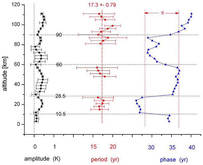
Figure 1 Vertical structures of long-period oscillations near 17.3±0.8 years from HAMMONIA temperatures. Missing period values could not be derived from the data. They were prescribed as the mean value of 17.3 years (dash–dotted vertical red line; see text and Sect. 3.2). Phases are relative values.

2.2 HAMMONIA

The HAMMONIA model (Schmidt et al., 2006) is based on the ECHAM5 general circulation model (Röckner et al., 2006) but extends the domain vertically to $\mathrm{2}\times {\mathrm{10}}^{-\mathrm{7}}$ hPa and is coupled to the MOZART3 chemistry scheme (Kinnison et al., 2007). The simulation analysed here was run at a spectral resolution of T31 with 119 vertical layers. The relatively high vertical resolution of less than 1 km in the stratosphere allows an internal generation of the QBO. Here we analyse the simulation (with fixed boundary conditions, including aerosol, ozone climatology) that was called “Hhi-max” in Offermann et al. (2015), but instead of only 11 we use 34 simulated years. Further details of the simulation are given by Schmidt et al. (2010).

As concerns the land parameters, part of them were also kept constant (vegetation parameters as leaf area, wood coverage) and so was ground albedo. Others were not (e.g. snow and ice on lakes). Hence, some influence on our oscillations is possible.

An example of the HAMMONIA data is given in Fig. 2 for 0 and 3 km altitudes. The HAMMONIA data were searched for long-period oscillations up to 110 km. The detailed analysis is described below (Sect. 3.2). Nine oscillations were identified with periods between 5.3 and 28.5 years. They are listed in Table 2a. The oscillation shown in Fig. 1 (17.3 years) is from about the middle of this range.

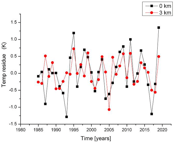
Figure 2 HAMMONIA temperature residues at 0 and 3 km altitude with fixed boundary conditions (see text). Mean temperatures of 281.89 K (0 km) and 266.04 K (3 km) have been subtracted from the model temperatures. Data are for 50^∘ N, 7^∘ E.

2.3 WACCM

Long runs with chemistry–climate models (CCMs) having restricted boundary conditions are not frequently available. A model run much longer than 34 years became available from the CESM-WACCM4 model. This 150-year run was analysed from the ground up to 108 km. The model experiments are described in Hansen et al. (2014). Here, the experiment with monthly varying constant climatological sea surface temperatures (SSTs) and sea ice has been used; i.e. there is a seasonal variation, but it is the same in all years. Other boundary conditions such as greenhouse gases (GHGs) and ozone-depleting substances (ODPs) were kept constant at 1960 values.

Solar cycle variability, however, was not kept constant during this model experiment. Spectrally resolved solar irradiance variability as well as variations in the total solar irradiance and the F10.7 cm solar radio flux were used from 1955 to 2004 from Lean et al. (2005). Thereafter solar variations from 1962–2004 were used as a block of proxy data and added to the data series several times to reach 150 years in total. Details are given in Matthes et al. (2013).

The WACCM data were analysed for long-period oscillations in the same manner as the HAMMONIA data. Here, the emphasis is on longer periods. Besides many shorter oscillations, nine oscillations with periods of more than 20 years were found. These results are included in Table 2a.

2.4 ECHAM6

The longest computer run available to us, covering 400 years, is from ECHAM6. ECHAM6 (Stevens et al., 2013) is the successor of ECHAM5, the base model of HAMMONIA. Major changes relative to ECHAM5 include an improved representation of radiative transfer in the solar part of the spectrum, a new description of atmospheric aerosol, and a new representation of the surface albedo. While the standard configuration of ECHAM5 used a model top at 10 hPa, this was extended to 0.01 hPa in ECHAM6. As the atmospheric component of the Max Planck Institute Earth System Model (MPI-ESM; Giorgetta et al., 2013), it has been used in a large number of model intercomparison studies related to the Coupled Model Intercomparison Project phase 5 (CMIP5). The ECHAM6 simulation analysed here was run at T63 spectral resolution with 47 vertical layers (not allowing for an internal generation of the QBO). All boundary conditions were fixed to constant values, taken as an average of the years 1979 to 2008.

The temperature data were analysed as the other data sets described above. Seventeen oscillation periods longer than 20 years were obtained (Table 2a). The ECHAM6 results in this paper are considered an approximate extension of the HAMMONIA results.

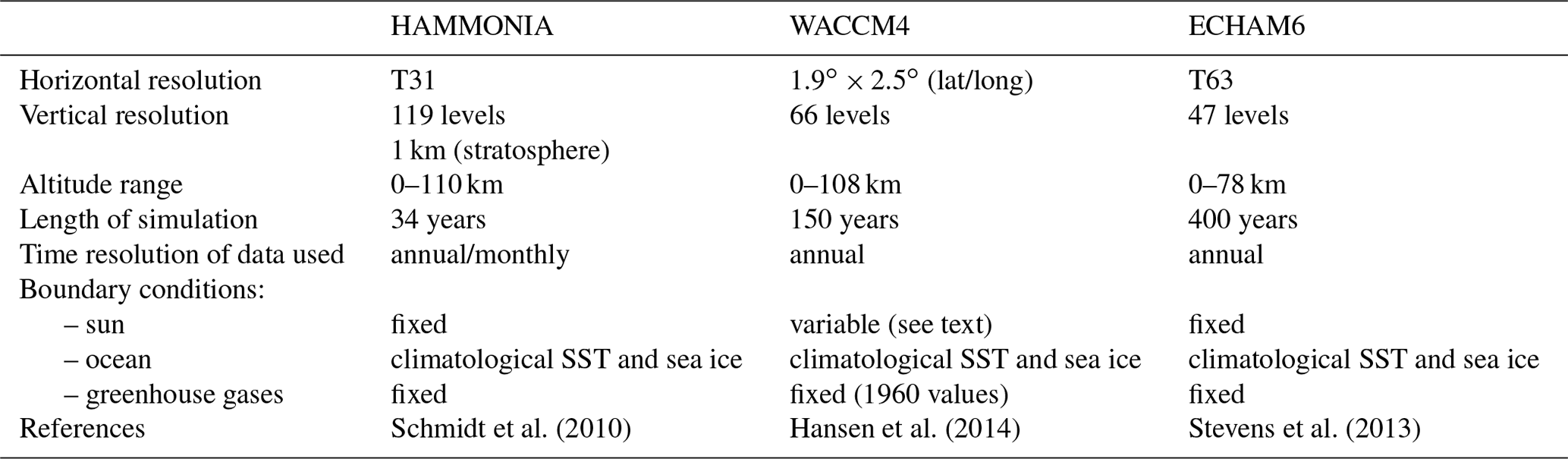
A summary of the model properties is given in Table 1. All analyses in this paper are for central Europe. The vertical model profiles are for 50^∘ N, 7^∘ E.

Table 1 Properties of the GCM simulations. All data are for central Europe (50^∘ N, 7^∘ E). For various details see text.

3 Model results

3.1 Vertical correlations of atmospheric temperatures

Figure 1 indicates that there are some vertical correlation structures in the atmospheric temperatures. This was studied in detail for the HAMMONIA and ECHAM6 data.

Ground temperature residues from the HAMMONIA run 38123 (34 years) are shown in Fig. 2 (black squares). The mean temperature is 281.89 K, which was subtracted from the model data. The boundary conditions (sun, ocean, greenhouse gases, soil humidity, land use, vegetation) have been kept constant, as discussed above. The temperature fluctuations thus show the atmospheric variability (standard deviation is σ=0.62 K). This variability is frequently termed “(climate) noise” in the literature. It will be checked whether this notion is justified in the present case.

Also shown in Fig. 2 are the corresponding HAMMONIA data for 3 km altitude. The mean temperature is 266.04 K; the standard deviation is σ=0.41 K. The statistical error of these two standard deviations is about 12 %. Hence the internal variances at the two altitudes are statistically different. This suggests that there may be a vertical structure in the variability that should be analysed.

The data sets in Fig. 2 show large changes within short times (2–4 years). Sometimes these changes are similar at the two altitudes. The variability of HAMMONIA thus appears to contain an appreciable high-frequency component and thus also needs to be analysed for vertical and for spectral structures.

Temperatures at layers 3 km apart in altitude were therefore correlated with those at 42 km as a reference altitude (near the stratopause). The results are shown in Fig. 3 for the HAMMONIA model run up to 105 km (red dots). A corresponding analysis for the much longer model run of ECHAM6 is also shown (black squares, up to 78 km). Two important results are obtained: (1) there is an oscillatory vertical structure in the correlation coefficient r with a maximum in the upper mesosphere and lower thermosphere and two minima in the lower stratosphere and in the mesosphere (for HAMMONIA). The correlations are highly significant near the upper three of these extrema (see the 95 % lines in Fig. 3). (2) The correlations in the two different data sets are nearly the same above the troposphere. This is remarkable because the two sets cover time intervals very different in length (34 years vs. 400 years). Therefore, the correlation structure appears to be a basic property of the atmosphere (see below).

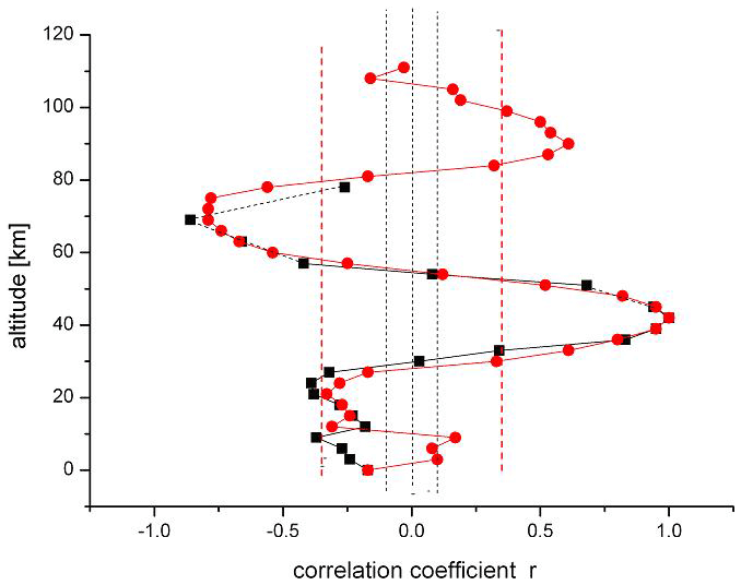
Figure 3 Vertical correlation of temperatures in HAMMONIA (red dots) and ECHAM6 (black squares). Reference altitude is 42 km (r=1). Vertical dashed lines show 95 % significance for HAMMONIA (red) and ECHAM6 (black).

The correlations suggest that the fluctuations in the atmosphere (or part of them) are somehow “synchronized” at adjacent altitude levels. A vertical (layered) structure might therefore be present in the magnitude of the fluctuations, too. This was studied by means of the standard deviations σ of the temperatures T; the result is shown in Fig. 4. There is indeed a vertical structure with fairly pronounced layers.

Figure 4 HAMMONIA temperatures: comparison of standard deviations (black squares, multiplied by 2 for easier comparison) and correlation coefficients (red dots, see Fig. 3). For details see text.

The HAMMONIA data used for Fig. 4 were annual data that have been smoothed by a four-point running mean. This was done to reduce the influence of high-frequency “noise” mentioned above, which is substantial (a factor of 2). The correlation calculations were repeated with the unsmoothed data. The results are essentially the same. The same applies to the standard deviations.

The layered structures shown in Figs. 3 and 4 are not unrelated. This can be seen in Fig. 4, which also gives the vertical correlations r (Fig. 3) for comparison. The horizontal dashed lines indicate that the maxima of the standard deviations occur near the extrema of the correlation profile in the stratosphere and lower mesosphere. This suggests that the fluctuations in adjacent σ maxima (and in adjacent layers) are anticorrelated. Surprisingly these anticorrelations are also approximately seen in the amplitude and phase profiles of Fig. 1 that are typical of all oscillations (see below).

The ECHAM6 data have been analysed in the same way as the HAMMONIA data, including a smoothing by a four-point running mean. The data cover the altitude range of 0–78 km for a 400-year simulation. The results are very similar to those of HAMMONIA. This is shown in Fig. 5, which gives vertical profiles of standard deviations and of vertical correlations of the smoothed ECHAM6 data and is to be compared to the HAMMONIA results in Fig. 4. The two upper maxima of standard deviations are again anticorrelated.

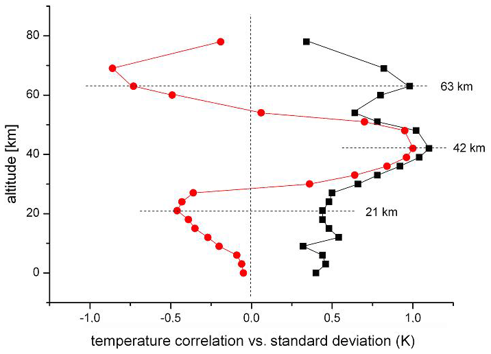
Figure 5 ECHAM6 temperatures: comparison of standard deviations (black squares, multiplied by 2) and correlation coefficients (red dots). For details see text.

It is apparently a basic property of the atmosphere's internal variability to be organized in some kind of “layers”, and that adjacent layers are anticorrelated. It appears therefore questionable whether the internal variability may be termed noise, as is frequently done in the literature.

3.2 Time structures

The correlations or anticorrelations concern temporal variations in temperatures. This suggests a search for some kind of regular (ordered) structure in the time series, as well. Therefore in a first step, FFT (fast Fourier transform) analyses have been performed for all HAMMONIA altitude levels (3 km apart). The results are shown in Fig. 6, which gives amplitudes for the period range of 4–34 years versus altitude. Also in this picture, the amplitudes show a layered structure. In addition an ordered structure in the period domain is also indicated. There are increased or high amplitudes near certain period values, for instance at the left- and right-hand side and in the middle of the picture. A similar result is obtained for the ECHAM6 data shown in Fig. 7 for the longer periods of 10–400 years. The layered structure in altitude is clearly seen, and so are the increased amplitudes near certain period values. Obviously, the computer simulations contain periodic temperature oscillations, the amplitudes of which show a vertically layered order.

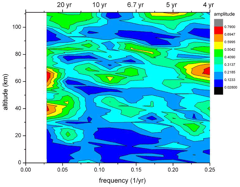
Figure 6 Long-period temperature oscillations in the HAMMONIA model. FFT amplitudes are shown in dependence on altitude and frequency (periods 4–34 years). Colour code of amplitudes is in arbitrary units.

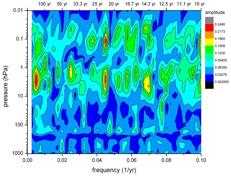
Figure 7 Long-period temperature oscillations in the ECHAM6 model. FFT amplitudes are shown in dependence on altitude and frequency (periods 10–400 years). Colour code of amplitudes is in arbitrary units.

The amplitudes shown in Figs. 6 and 7 are relative values, and the resolution of the spectra is quite limited. Therefore a more detailed analysis is required. For this purpose the Lomb–Scargle periodogram (Lomb, 1976; Scargle, 1982) is used. As an example Fig. 8 shows the mean Lomb–Scargle periodogram in the period range 20–100 years for the ECHAM6 data. For this picture Lomb–Scargle spectra were calculated for all ECHAM6 layers separately, and the mean spectrum of all altitudes was determined. The power of the periodogram gives the reduction in the sum of squares when fitting a sinusoid to the data (Scargle, 1982); i.e. it is equivalent to a harmonic analysis using least-square fitting of sinusoids. The power values are normalized by the variance of the data to obtain comparability of the layers with different variance. Quite a number of spectral peaks are seen between 20- and 60-year periods. Further oscillations appear to be present around 100 years and at even longer periods (not shown here as they are not sufficiently resolved).

Figure 8 Long-period temperature oscillations in the ECHAM6 model Lomb–Scargle periodogram is given for periods of 20–100 years. Dashed red line indicates significance at the 2σ level. For straight red line see text.

We compared the mean result for the ECHAM6 data with 10 000 representations of noise. One representation covers 47 atmospheric layers. For each representation we took noise from a Gaussian distribution for each atmospheric layer independently and calculated a mean Lomb–Scargle periodogram for every representation in the same way as for the ECHAM6 data.

It might be considered appropriate to use red noise instead of white noise in this analysis. We therefore calculated the sample autocorrelation at a lag of 1 year for the different ECHAM6 altitudes. These values were found to be very close to zero and, thus, we used Gaussian noise in our analysis.

The red line in Fig. 8 shows the average of all of these mean periodograms. As expected for the average of all representations, the peaks cancel, and one gets an approximately constant value for all periods. A single representation typically shows one or several peaks above this mean level. The red dashed line gives the upper 2σ level, i.e. the mean plus 2σ. As the mean Lomb–Scargle periodogram for the ECHAM6 data shows several peaks clearly above this upper 2σ level, this mean periodogram is significantly different from that of independent noise. Therefore, the conclusion is that independent noise at the different atmospheric layers alone cannot explain the observed periodogram showing large remaining peaks after averaging.

Table 2 Periods of temperature oscillations from harmonic analyses. (a) Periods are numbered according to increasing values. Periods (in years) are given with their standard deviations. Modelled periods are from the HAMMONIA, WACCM, and ECHAM6 models, respectively. Additional periods are from Hohenpeißenberg measurements and from the Global Land Ocean Temperature Index (GLOTI). HAMMONIA periods are limited to 28.5 years as the model run covered 34 years, only. WACCM periods are given for less than 147 years from a model run of 150 years. ECHAM6 periods are from a 400-year run. Short periods (below 20 years) are not shown for WACCM, ECHAM6, and GLOTI as they are not used in the present paper. Hohenpeißenberg and GLOTI data after 1980 are not included in the analyses because of their steep increase in later years. Periods given in bold type refer to (b). (b) Comparative periods (in years).

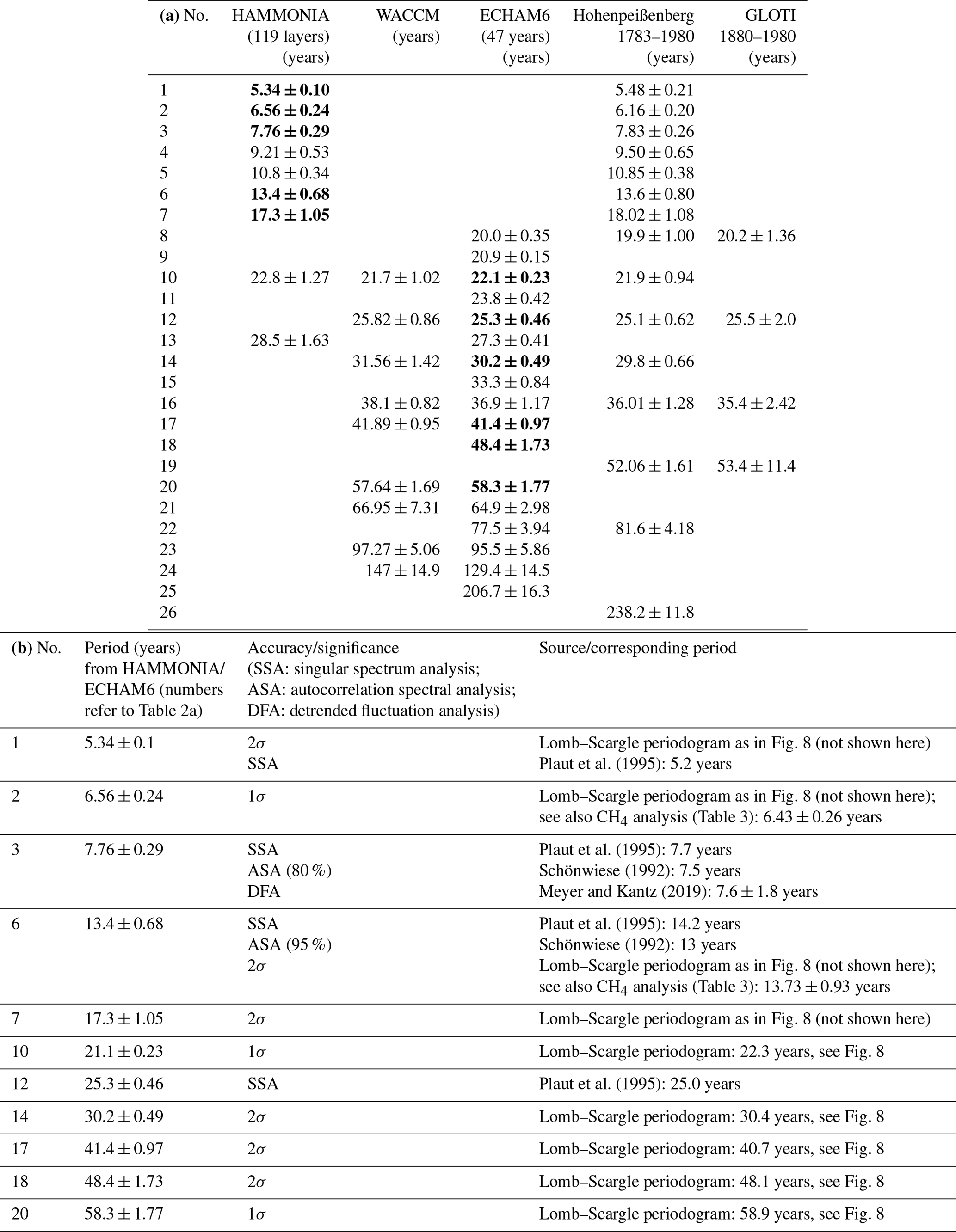
The period values shown in Fig. 8 agree with those given for ECHAM6 in Table 2a which are from the harmonic analysis described next. The agreement is within the error bars given in Table 2a (except for 24.3 years).

A spectral analysis such as that in Fig. 8 was also performed for the HAMMONIA temperatures. It showed the periods of 5.3 and 17.3 years above the 2σ level. These values agree within single error bars with those given in Table 2a. All peaks found to be significant (in different analyses) are marked by heavy print in Table 2a.

The Lomb–Scargle spectra (in their original form) do not reveal the phases of the oscillations. We have therefore applied harmonic analyses to our data series. This was done by stepping through the period domain in steps 10 % apart. In each step we looked for the largest nearby sinus oscillation peak. This was done by means of an ORIGIN search algorithm (ORIGIN Pro 8G, Levenberg–Marquardt algorithm) that yielded optimum values for period, amplitude, and phase. The algorithm starts from a given initial period and looks for a major oscillation in its vicinity. For this it determines period, amplitude , and phase, including error bars. If in this paper the term “harmonic analysis” is used, this algorithm is always meant. The results are a first approximation, though, because only one period was fitted at a time, instead of the whole spectrum. Furthermore, the 10 % grid may be sometimes too coarse. Also small-amplitude oscillations may be overlooked.

This analysis was performed for all altitude levels available. Figure 1 shows an example for the HAMMONIA temperatures from 3–111 km for periods around 15–20 years. The middle track (red dots) shows the periods with their error bars, the left side shows the amplitudes, and the right side shows the phases. The mean of all periods is 17.3±0.79 years. There are several altitudes where the harmonic analysis does not give a period. This may occur if an amplitude is very small or if there is a nearby period with a strong amplitude that masks the smaller one. At these altitudes the periods were interpolated for the fit (dash–dotted vertical line). The mean of the derived periods (17.3 years) is used as an estimated interpolation value. This is because the derived periods do not deviate too much from the mean value. This procedure allows us to obtain estimated amplitude and phase values for instance in the vicinity of the amplitude minima. That is important because at these altitudes large phase changes are frequently observed. The Levenberg–Marquardt algorithm calculates an amplitude and phase if a prescribed (estimated) period is provided.

The right track in Fig. 1 shows the phases of the oscillations. The special feature about this vertical profile is its step-like structure with almost constant values in some altitudes and a subsequent fast change somewhat higher to some other constant level. These changes are about 180^∘ (π); i.e. the temperatures above and below these levels are anticorrelated. At these levels the temperature amplitudes (left track) are at a minimum, with maxima in between. These maxima occur near the altitudes of the maxima of the temperature standard deviations in Fig. 4 that are anticorrelated in adjacent layers. The phase steps in Fig. 1 approximately fit this picture. They suggest that the layer anticorrelation discussed above corresponds at least in part to the phase structure of the long-period oscillations in the atmosphere.

This important result was checked by an analysis of other oscillations contained in the HAMMONIA data series. Nine oscillations with periods between 5.34 and 28.5 years were obtained by the analysis procedure described above. They are listed in Table 2a, and all show vertical profiles similarly as in Fig. 1.

Figure 1 shows that at different altitudes the periods are somewhat different. They cluster, however, quite closely about their mean value of 17.3 years. This clustering about a mean value is found for almost all periods listed in Table 2a. This is shown in detail in Figs. 9 and 10, which give the number of periods found at different altitudes in a fixed period interval. The clusters are separated by major gaps, as is indicated by vertical dashed lines (black). This suggests using a mean period value as an estimate of the oscillation period representative of all altitudes. The mean period values are given above each cluster in red, together with a red solid line. A few clusters are not very pronounced, and hence the corresponding mean period values are unreliable (e.g. those beyond 20 years; see the increased standard deviations in Table 2a).

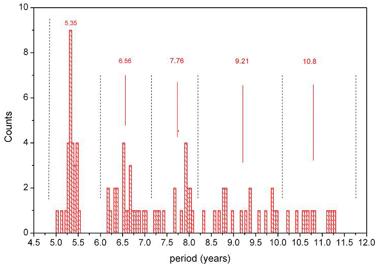
Figure 9 Number of oscillations counted in a fixed period interval at periods 4.75–11.75 years. Interval is 0.05 years (HAMMONIA).

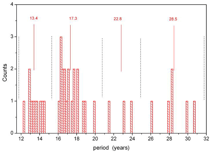
Figure 10 Number of oscillations counted in a fixed period interval at periods 11.75–31.75 years. Interval is 0.2 years (HAMMONIA).

In determining the mean oscillation periods we have avoided subjective influences as follows: periods obtained at various altitudes were plotted versus altitude as shown in Fig. 1 (middle column, red). When covering the period range of 5 to 30 years, nine vertical columns appeared. The definition criterion of the columns was that there should not be any overlap between adjacent columns. It turned out that such an attribution was possible. To make this visible we have plotted the histograms in Figs. 9 and 10. The pictures show that the column values form the clusters mentioned, which are separated by gaps. The gaps that are the largest ones in the neighbourhood of a peak are used as boundaries (except at 7.15 years). It turns out that if an oscillation value near a boundary is tentatively shifted from one cluster to the neighbouring one, the mean cluster values experience only minor changes. Figure 10 shows that our procedure comes to its limits, however, for periods longer than 20 years (for HAMMONIA). This is seen in Table 2a from the large error bars. We still include these values for illustration and completeness.

It is important to note that all HAMMONIA values in Table 2a (except 28.5 years) agree with the Hohenpeißenberg values within the combined error bars. The Hohenpeißenberg data are ground values and hence not subject to our clustering procedure. Furthermore also all other model periods in Table 2a have been derived by the same cluster procedure. The close agreement discussed in the text suggests that this technique is reliable.

ECHAM6 data are used in the present paper to analyse much longer time windows (400 years) than of HAMMONIA (34 years). Results shown in Figs. 3, 5, and 7 are quite similar to those of HAMMONIA. Harmonic analysis of long oscillation periods was performed in the same way as for HAMMONIA. Seventeen periods were found to be longer than 20 years and have been included in Table 2a. Shorter periods are not shown here as that range is covered by HAMMONIA. The amplitude and phase structures of these are very similar to those of HAMMONIA. The cluster formation about the mean period values is also obtained for ECHAM6 and looks quite similar to Figs. 9 and 10.

The vertical amplitude and phase profiles of the mean periods given in Table 2a all show intermittent amplitude maxima or minima and step-like phase structures. In general, they look very similar to Fig. 1. We have calculated the accumulated amplitudes (sums) from all of these profiles at all altitudes. They are shown in Fig. 11a for HAMMONIA. They clearly show a layered structure similar to the temperature standard deviations in Fig. 4, with maxima at altitudes close to those of the standard deviation maxima. The figure also closely corresponds to the amplitude distribution shown in Fig. 1, with maxima and minima occurring at similar altitudes in either picture.

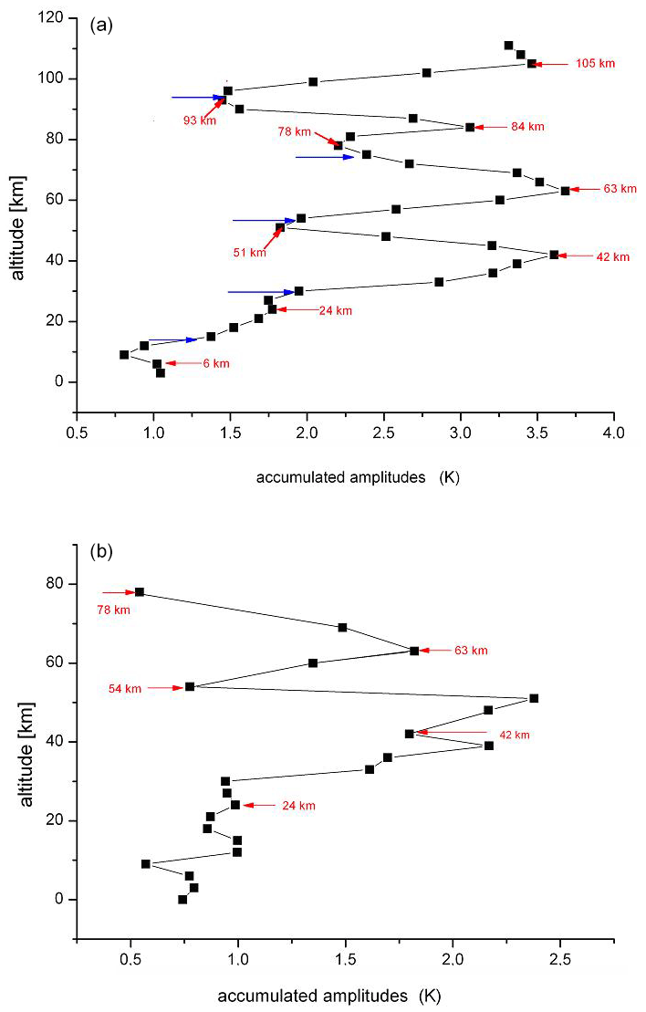
Figure 11 (a) Long-period temperature oscillations in the HAMMONIA model. Accumulated amplitudes are shown vs. altitude for periods of 5.3–28.5 years (see Table 2a). Blue horizontal arrows show mean altitudes of phase jumps. Red arrows indicate altitudes of maxima and minima. (b) Long-period temperature oscillations in the ECHAM6 model. Accumulated amplitudes are shown vs. altitude for the periods given in Table 2a. Red arrows indicate altitudes of maxima and minima.

Accumulated amplitudes have also been calculated for the ECHAM6 periods, and similar results are obtained as for HAMMONIA (see Fig. 11b). The similarity is already indicated in Fig. 3 above 15 km. The correlation of the HAMMONIA and ECHAM6 curves above this altitude has a correlation coefficient of 0.97. This and Fig. 11 support the idea that all of our long-period oscillations have a similar vertical amplitude structure.

The phase jumps in the nine oscillation vertical profiles of HAMMONIA also occur at similar altitudes. Therefore the mean altitudes of these jumps have been calculated and are shown in Fig. 11a as blue horizontal arrows. They are seen to be close to the minima of the accumulated amplitudes and thus confirm the anticorrelations between adjacent layers. Figures 4, 1, and 11 thus show a general structure of temperature correlations or anticorrelations between different layers of the HAMMONIA atmosphere and suggest the phase structure of the oscillations as an explanation. The same is valid for ECHAM6.

Altogether HAMMONIA and ECHAM6 consistently show the same type of variability and oscillation structures. This type occurs in a wide time domain of 400 years. As mentioned, we do not believe that these ordered structures are adequately described by the term “noise”, as this notion is normally used for something occurring at random.

3.3 Intrinsic oscillation periods

Three different model runs of different lengths have been investigated by the harmonic analysis described. The HAMMONIA model covered 34 years, the WACCM model covered 150 years, and the ECHAM6 model covered 400 years. The intention was to study the differences resulting from the different nature of the models, and from the difference in the length of the model runs.

The oscillation periods found in these model runs are listed in Table 2a. These periods are vertical mean values as described for Figs. 1 and 9–10. Periods are given in order of increasing values in years together with their standard deviations. Only periods longer than 5 years are shown here. The maximum period cannot be longer than the length of the computer run. Therefore, the number of periods to be found in a model run can – in principle – be larger the longer the length of the run is. Table 2a preferentially shows periods longer than 20 years (except for HAMMONIA and Hohenpeißenberg) as the emphasis is on the long periods here. Of course, periods comparable to the length of the data series need to be considered with caution.

The periods shown here at a given altitude are from the Levenberg–Marquardt algorithm (at 1σ significance). The values obtained at different altitudes in a given model have been averaged as described above, and the corresponding mean and its standard error are given in Table 2a.

Table 2a also contains two columns of periods and their standard deviations that were derived from measured temperatures. These are data obtained on the ground at the Hohenpeißenberg Observatory (47.8^∘ N, 11.0^∘ E) from 1783 to 1980 and are globally averaged GLOTI data (Hansen et al., 2010). The data are annual mean values smoothed by a 16-point running mean and will be discussed below. Data after 1980 are not included in the harmonic analyses because they steeply increase thereafter (“climate change”). The periods are determined as for the data of the other rows of Table 2a (see Sect. 3.2).

The Hohenpeißenberg and GLOTI periods show several close agreements with the HAMMONIA and ECHAM6 results. Further comparisons with other data analyses are given below. A summary is given in Table 2b. Different techniques have been used, such as singular spectrum analysis (SSA), autocorrelation spectral analysis (ASA), and detrended fluctuation analysis (DFA), and yield similar results. They are also shown in Table 2b. For the accuracy and significance of these techniques the reader is referred to the corresponding papers. The periods listed in Table 2b are given in bold type in Table 2a.

There are some empty spaces in the lists of Table 2a. It is believed that this is because these oscillations are not excited in that model run or that their excitation is not strong enough to be detected or that the spectral resolution of the data series is insufficient (strong changes in amplitudes strengths are, for instance, seen in Fig. 1). For the measured data in Table 2a it needs to be kept in mind that they were under the influence of varying boundary conditions.

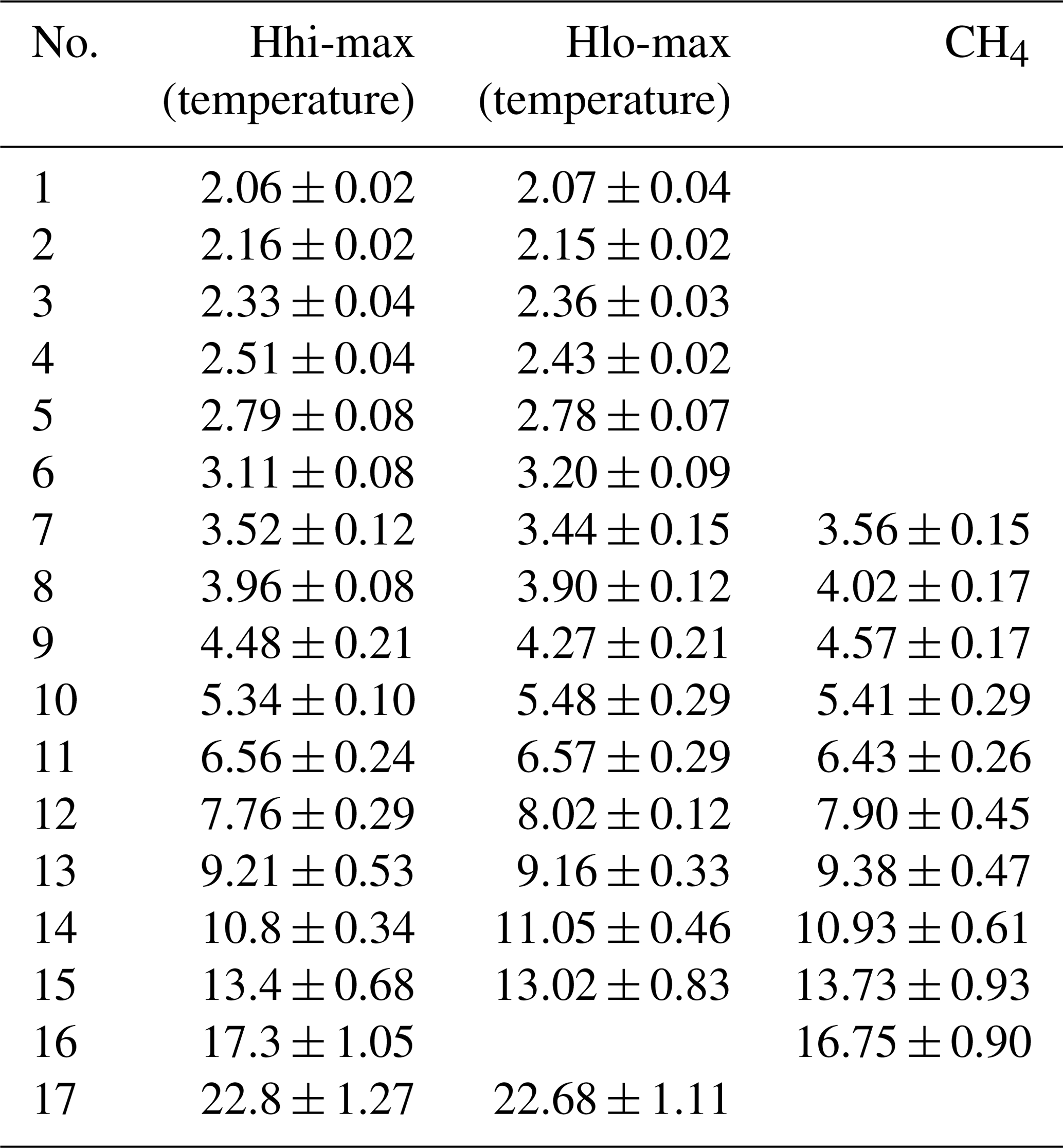
The model runs shown in Table 2a have different altitude resolutions. The best resolution (1 km) is available in HAMMONIA (119 vertical layers, run Hhi-max in the earlier paper of Offermann et al., 2015). The very long run of ECHAM6 uses only 47 layers. Data on a 3 km altitude grid are used here. In the earlier paper it was shown on the basis of a limited data set (HAMMONIA, Hlo-max) that a decrease in the number of layers affected the vertical amplitude and phase profiles of the oscillations found. It did, however, not change the oscillation periods. For a more detailed analysis a 20-year-long run of Hlo-max (67 layers) is now compared to the 34-year-long run of Hhi-max (119 layers). The resulting oscillation periods are shown in Table 3 (together with their standard deviations). Sixteen pairs of periods are listed that all agree within the single error bars (except no. 4). Hence it is confirmed that the periods of the oscillations are quite robust with respect to changes in altitude resolution. The periods of the ECHAM6 run can therefore be regarded as reliable, despite their limited altitude resolution.

Table 3 Period comparison of two different HAMMONIA runs: temperature and CH₄. Periods (in years) are given together with their standard deviations. HAMMONIA run Hhi-max (temperature and CH₄ mixing ratios) uses 119 altitude layers and covers 34 years; run Hlo-max uses 67 layers and covers 20 years.

When comparing the periods in Table 2a to each other several surprising agreements are observed. It turns out that all periods of the HAMMONIA and WACCM models find a counterpart in the ECHAM6 data (not vice versa). These data pairs always agree within their combined error bars and mostly even within single error bars. The difference between the members of a pair is much smaller than the distance to any neighbouring value with a higher or lower ordering number in Table 2a. From this it is concluded that the different models find the same oscillations. Their periods are obviously quite robust.

A similar agreement is seen for the periods found in the measured Hohenpeißenberg data. These have been under the influence of variations in the sun, ocean, and greenhouse gases. A spectral analysis (autocorrelation spectral analysis) of these data is shown in Fig. 12. It was taken from Schönwiese (1992). The important peak at 3.4 years is not contained in Table 2 but was found in Offermann et al. (2015). The two peaks near 7.5 and 13 years are close to the values of 7.76±0.29 and 13.4±0.68 years in Table 2a.

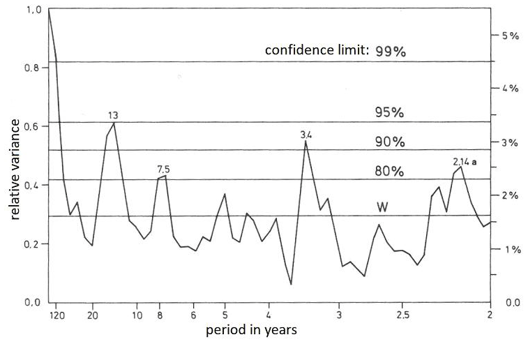
Figure 12 Periodogram (2 to 120 years) of measured Hohenpeißenberg temperatures from Schönwiese (1992, Fig. 57). Results are from an autocorrelation spectral analysis ASA.

A 335-year-long data set of central England temperatures (CETs) is the longest measured temperature series available (Plaut et al., 1995). A singular spectrum analysis was applied by these authors for interannual and interdecadal periods. Periods of 25.0, 14.2, 7.7, and 5.2 years were identified. All of these values nearly agree with numbers given for HAMMONIA, WACCM, and/or ECHAM6 in Table 2a (within the error bars given in the table).

Meyer and Kantz (2019) recently studied the data from a large number of European stations by the method of detrended fluctuation analysis. They identified a period of 7.6±1.8 years, which again is in agreement with the HAMMONIA results given in Table 2a (and also agrees with Fig. 12 and with Plaut et al., 1995).

Also the GLOTI data in Table 2a are in agreement with some of the other periods, even though they are global averages. It will be shown below that such results are not limited to atmospheric temperatures alone but are, for instance, also seen in methane mixing ratios.

3.4 Oscillation amplitudes

In an attempt to learn more about the nature of the long-period oscillations we analyse their oscillation amplitudes. The calculation of absolute amplitudes is difficult and beyond the scope of the present paper. However, interesting results can be obtained from their relative values. One of these results is related to the vertical gradients of the atmospheric temperature profiles.

The HAMMONIA model simulates the atmospheric structure as a whole. The annual mean vertical profile of HAMMONIA temperatures can be derived and is seen to vary between a minimum at the tropopause, a maximum at the stratopause, and another minimum near the mesopause (not shown here). In consequence the vertical temperature gradients change from positive to negative and to positive again. This is shown in Fig. 13 (red dots) between 18 and 96 km. The temperature gradients are approximated by the temperature differences in consecutive levels.

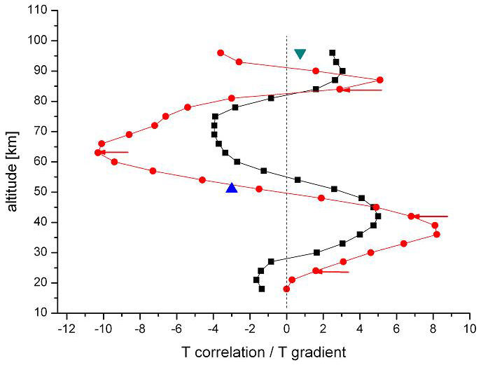
Figure 13 Comparison of HAMMONIA vertical correlations from Fig. 3 (black squares) with vertical temperature gradients (red dots). Data are from annual mean temperatures. Correlation coefficients are multiplied by 5. Temperature gradients are approximated by the differences in consecutive temperatures (K per 3 km). Two additional gradients are given for monthly mean temperature curves: blue triangle for January, green inverted triangle for July. Red arrows show the altitudes of the maxima of the accumulated amplitudes in Fig. 11a.

Also shown in Fig. 13 is the correlation profile of HAMMONIA from Fig. 3 (black squares here). The two curves are surprisingly similar. The similarity suggests some connection of the oscillation structure and the mean thermal structure of the middle atmosphere. This is shown more clearly by the accumulated amplitudes of the long-period oscillations in Fig. 11a. The maxima of these occur at altitudes near the extrema of the temperature gradients as is shown by the red arrows in Fig. 13. The mechanism connecting the oscillations and the thermal structure appears to be active throughout the whole altitude range shown (except the lowest altitudes).

A possible mechanism might be a vertical displacement of air parcels. If an air column is displaced vertically by some distance D (“displacement height”), a seeming change in mixing ratio is observed at a given altitude. This is a relative change only, not a photochemical one. It can be estimated by the product D times mixing ratio gradient. If the vertical movement is an oscillation, the trace gas variation is an oscillation as well, assuming that D is a constant. Such transports may be best studied by means of a trace gas like CH₄.

HAMMONIA methane mixing ratios have therefore been investigated for oscillation periods in the same way as described above for the temperatures. Results are briefly summarized here.

Indeed, 10 periods have been found between 3.56 and 16.75 years by harmonic analyses and are shown in Table 3. These periods are very similar to those obtained for the temperatures in Tables 2a and 3. The agreement is within the single error bars. Hence it is concluded that the same oscillations are seen in HAMMONIA temperatures and CH₄ mixing ratios.

The CH₄ oscillations support the idea that a displacement mechanism is active. The corresponding displacement heights D were estimated from the CH₄ amplitudes and the vertical gradients of the mean HAMMONIA CH₄ mixing ratios.

The values D obtained from the different oscillation periods are about the same, though they show some scatter. This makes us presume that the displacement mechanism may be the same for all oscillations. The values D appear to follow a trend in the vertical direction. The displacements are below 100 m in the lower stratosphere and slowly increase with height to above 200 m.

Thus the important result is obtained that the our long-period oscillations are related to a vertical displacement mechanism that is altitude dependent but appears to be the same for all periods. A more detailed analysis is beyond the scope of this paper.

3.5 Seasonal aspects

Our analysis has so far been restricted to annual mean values. Large temperature variations on much shorter timescales are also known to occur in the atmosphere, including vertical correlations (e.g. seasonal variations). This suggests the question of whether these might be somehow related to the long-period oscillations. Our spectral analysis is therefore repeated using monthly mean temperatures of HAMMONIA.

Results are shown in Figs. 14 and 15, which give the amplitude distribution vs. period and altitude of FFT analyses for the months of July and January. These two months are typical of summer (May–August) and winter (November–March), respectively. In July oscillation amplitudes are seen essentially at altitudes above about 80 km and some below about 20 km. In the regime in between, oscillations are obviously very small or not excited. The opposite behaviour is seen in January: oscillation amplitudes are now observed in the middle-altitude regime where they had been absent in July. This is to be compared to Figs. 6 and 11 that give the annual mean picture. In Fig. 11 the structures (two peaks) above 80 km appear to represent the summer months (Fig. 14). The structures between 80 and 30 km, on the other hand, apparently are representative of the winter months (Fig. 15).

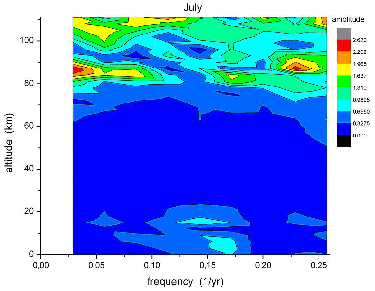
Figure 14 Long-period temperature oscillations in the month of July in HAMMONIA. Amplitudes are shown in dependence of altitude and frequency (periods 3.9–34 years). Colour code of amplitudes is in arbitrary units.

Figure 15 Long-period temperature oscillations as in Fig. 14 but for the month of January.

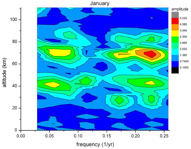
The monthly oscillations appear to be related to the wind field of the HAMMONIA model. Figure 16 shows the monthly zonal winds of HAMMONIA from the ground up to 111 km (50^∘ N). Comparison with Figs. 14 and 15 shows that oscillation amplitudes are obviously not observed in an easterly wind regime. Hence, the long-period oscillations and their phase changes are apparently related to the dynamical structure of the middle atmosphere. A change from high to low oscillation activity in the vertical direction appears to be related to a wind reversal.

Figure 16 Vertical distribution of zonal wind speed in the HAMMONIA model.

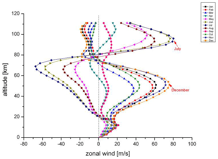
This correspondence does not, however, exist in all details. In the regimes of oscillation activity there are substructures. For instance in the middle of the July regime of amplitudes above 80 km, there is a “valley” of low values at about 95 km. A similar valley is seen in the January data around 55 km. Near these altitudes there are phase changes of about 180^∘ (see the blue arrows in Fig. 11a). Contrary to our expectation sketched above, these are altitudes of large westerly zonal wind speeds without much vertical change (see Fig. 16). However, the two valleys are relatively close to altitudes where the vertical temperature gradients are small (see Fig. 13). As the gradients from the annual mean temperatures used for the curves in Fig. 13 may differ somewhat from the corresponding monthly values, two monthly gradients have been added in Fig. 13 for January (at 51 km) and for July (at 96 km). They are small, indeed, and could explain low oscillation amplitudes by the above-discussed vertical displacement mechanism.

3.6 Oscillation persistence

It is an important question whether the excitation of our oscillations is continuous or intermittent. To check on this we have subdivided the 400-year data record of ECHAM6 in four smaller time intervals (blocks) of 100 years each. In each block we performed harmonic analyses for periods of 24 years (frequency of 0.042/year) and 37 years (frequency of 0.027/year), respectively, at the altitudes of 42 km (1.9 hPa) and 63 km (0.11 hPa). These are altitudes and periods with strong signals as seen in Fig. 7. Results for the two altitudes and two periods are given in Fig. 17.

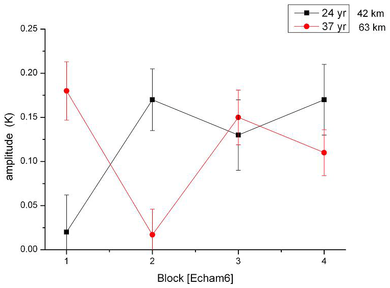
Figure 17 Amplitudes of 24 and 37 years oscillations in four subsequent equal time intervals (blocks) of the 400-year data set of ECHAM6.

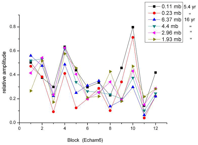
Figure 18 FFT amplitudes of 5.4- and 16-year oscillations in 12 equal time intervals (32-year blocks) of the ECHAM6 400-year data set.

The results show two groups of amplitudes: one is around 0.15 K; the other is very small and compatible with zero. The two groups are significantly different as is seen from the error bars. This result is compatible with the picture of oscillations being excited and not excited (dissipated) at different times. The non-excitation (dissipation) for the 24-year oscillation (black squares) occurs in the first block (century), that for the 37-year oscillation (red dots) in the second block. The 24-year profile at 63 km altitude is similar as that at 24 km. Likewise, the 37-year profile at 24 km is similar to that at 63 km. Hence it appears that the whole atmosphere (or a large part of it) is excited (or dissipated) simultaneously. (The two profiles in Fig. 17 appear to be somehow anticorrelated for some reason that is unknown as yet.)

For the analysis of shorter periods, the 400-year data set of ECHAM6 may be subdivided into a larger number of time intervals. Figure 18 shows the results for periods of 5.4 and 16 years, for various altitudes. An FFT analysis was performed at 12 equal time intervals (blocks of 32-year length) in the altitude regime 0.01–1000 hPa and the period regime 4–40 years. The corresponding 12 maps look similar to Fig. 15; i.e. there are pronounced amplitude hotspots at various altitudes and periods. (Of course, the values near the 40-year boundary are not really meaningful.) In subsequent blocks these hotspots may shift somewhat in altitude and/or period, and hence the profiles taken at a fixed period and altitude such as those of Fig. 18 show some scatter. Nevertheless, there is a strong indication of the occurrence of coordinated high maxima and deep minima of amplitudes in blocks 3 and 4 and blocks 10 and 11, respectively. These maxima are interpreted as strong oscillation excitation, whereas the minima are believed to show (at least in part) the dissipation of the oscillations.

It should be mentioned that in the FFT analysis the 5.4-year period is an overtone of the 16-year period. Hence the two period data in Fig. 18 may be related somehow.

4 Discussion

The long-period oscillations are seen in measurements as well as in model calculations.

The nature and origin of them are as yet unknown. We therefore collect here as many of their properties as possible.

4.1 Oscillation properties and possible self-excitation

The oscillations exist in computer models even if the model boundaries for the influences of the sun, the ocean, and the greenhouse gases are kept constant. Therefore one might suspect that they are self-generated. The oscillation periods are robust, which is typical of self-excited oscillations. However, external excitation by land surface processes is a possibility.

Further oscillation properties are as follows: the periods cover a wide range from 2 to more than 200 years (at least). The different oscillations have similar vertical profiles (up to 110 km) of amplitudes and phases. This may indicate three-dimensional atmospheric oscillation modes. To clarify this, latitudinal and longitudinal studies of the oscillations are needed in a future analysis.

4.2 Vertical layered amplitude structures and displacement mechanism

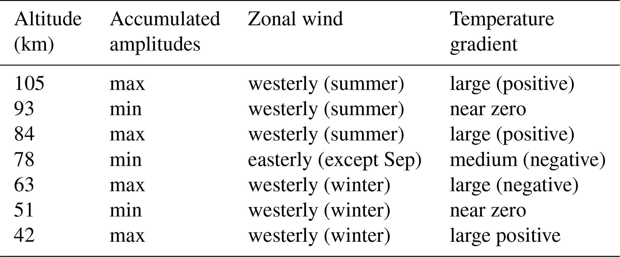
The accumulated oscillation amplitudes show a layer structure with alternating maxima and minima and correlations or anticorrelations in the vertical direction. These appear to be influenced by the seasonal variations in temperature and zonal wind in the stratosphere, mesosphere, and lower thermosphere. Table 4 summarizes the results shown in Sect. 3.5. Maxima of oscillation amplitudes appear to be associated with westerly (eastward) winds together with large temperature gradients (positive or negative). Amplitude minima are associated with either easterly (westward) winds or with near-zero temperature gradients. The latter feature is compatible with a possible vertical displacement mechanism. Indeed, such displacements can be seen in the CH₄ data of the HAMMONIA model. The mechanism summarized in Table 4 appears to be a basic feature of the atmosphere that influences many different parameters such as temperature and mixing ratios. Vertical displacements of measured temperature profiles have been discussed for instance by Kalicinsky et al. (2018).

Table 4 Maxima or minima of accumulated amplitudes of temperature oscillations and associated structures (see Fig. 11a) (stratosphere, mesosphere, lower thermosphere).

4.3 Oscillations are not noise!

The amplitudes found for the long-period oscillations are relatively small (Fig. 1). The question therefore arises whether these oscillations might be spurious peaks, i.e. some sort of noise. We tend to answer the question in the negative for the following reasons:

• a.

  An accidental agreement of periods as close together as those shown in Table 2a for different model computations appears very unlikely. This also applies to the Hohenpeißenberg data in Table 2a, and several of these periods are even found in the GLOTI data.

  If the period values were accidental, they should be evenly distributed over the period-space. To study this the range of ECHAM6 periods is considered. Table 2a shows that the error bars (standard deviations) of ECHAM6 cover approximately half of this range. If the periods of this and some other data set occur at random, half of them should coincide with the ECHAM6 periods within the ECHAM6 error bars, and half of them should not. This is checked by means of the WACCM model data, the Hohenpeissenberg measured data, and three further measurements sets that reach back to 1783 (Innsbruck, 47.3^∘ N, 11.4^∘ E; Vienna, 48.3^∘ N, 16.4^∘ E; Stockholm, 59.4^∘ N, 18.1^∘ E). The result is that about two-thirds of the periods coincide with ECHAM6 periods within the ECHAM6 error bars. This is far from an even distribution.

  It is important to note that the data sets used here are quite different in nature: they are either model simulations with fixed or partially fixed boundaries, or they are real atmospheric measurements at different locations.

  A further argument against noise is the distribution of the data in Figs. 9 and 10. If our oscillations were noise, the counts in these figures should be evenly distributed with respect to the period scale. However, the distribution is highly uneven, with high peaks and large gaps, which is very unlikely to result from noise.

• b.

  The periods given in Table 2a were all calculated by means of harmonic analyses (Levenberg–Marquardt algorithm). This was done to support the reliability of the comparison of the three models and four measured data sets. There could be, however, the risk of a “common mode failure”. The harmonic analysis results are therefore checked and are confirmed by the Lomb–Scargle analysis and ASA shown in Figs. 8 and 12 and by the above-cited results of Plaut et al. (1995) and Meyer and Kantz (2019). There is, however, no one-to-one correspondence of these numbers and those in Table 2a. In general the number of oscillations found by the harmonic analysis is larger. Hence several of the Table 2a periods might be considered questionable. It is also not certain that Table 2a is exhaustive. Nevertheless, the large number of close coincidences is surprising.

• c.

  The layered structure of the occurrence of the oscillations (e.g. Fig. 11a) and the corresponding anticorrelations appears impossible to reconcile with a noise field. These correlations extend over about 20 km (or more) in the vertical, which is about three scale heights. Turbulent correlation would, however, be expected over one transport length, i.e. one scale height, only.

• d.

  The apparent relation of the oscillations to the zonal wind field and the vertical temperature structure (Table 4) would be very difficult to explain by noise.

• e.

  The close agreement (within single error bars) of the oscillation periods in temperatures and in CH₄ mixing ratios would also be very difficult to explain by noise.

In summary it appears that many of the oscillations are intrinsic properties of the atmosphere that are also found in sophisticated simulations of the atmosphere.

4.4 Other atmospheric parameters

The long-period oscillations are studied here mainly for atmospheric temperatures. They show up, however, in a similar way in other parameters such as winds, pressure, trace gas densities, and NAO (Offermann et al., 2015). Some of the periods in Table 2a appear to be similar to the internal decadal variability of the atmosphere–ocean system (e.g. Meehl et al., 2013, 2016; Fyfe et al., 2016). One example is the Atlantic Multidecadal Oscillation (AMO) as discussed by Deser et al. (2010) with timescales of 65–80 years and with its “precise nature… still being refined”. Variability on centennial timescales and its internal forcing were recently discussed by Dijkstra and von der Heydt (2017). It needs to be emphasized that the oscillations discussed in the present paper are not caused by the ocean as they occur even if the ocean boundaries are kept constant.

4.5 Relation to “climate noise”

The long-period oscillations obviously are somehow related to the “internal variability” discussed in the atmosphere–ocean literature at 40–80-year timescales (“climate noise”; see, e.g., Deser et al., 2012; Gray et al., 2004, and other references in Sect. 1). The particular result of the present analysis is its extent from the ground up to 110 km, showing systematic structures in all of this altitude regime. These vertical structures lead us to hope that the nature of the oscillations and hence of (part of) the internal variability can be revealed in the future.

4.6 Time persistency

It appears that the time persistency of the long-period oscillations is limited. Longer data sets are needed to study this further.

4.7 Relation to climate change

The internal variability in the atmosphere–ocean system “makes an appreciable contribution to the total… uncertainty in the future (simulated) climate response” (Deser et al., 2012). Similarly our long-period oscillations might interfere with long-term (trend) analyses of various atmospheric parameters. This includes slow temperature increases as part of the long-term climate change and needs to be studied further.

5 Summary and conclusions

The atmospheric oscillation structures analysed in this paper occur in a similar way in different atmospheric climate models and even when the boundary conditions of sun, ocean, and greenhouse gases are kept constant. They also occur in long-term temperature measurements series. They are characterized by a large range of period values from below 5 to beyond 200 years.

As we do not yet understand the nature of the oscillations we try to assemble as many of their properties as possible. The oscillations show typical and consistent structures in their vertical profiles. Temperature amplitudes show a layered behaviour in the vertical direction with alternating maxima and minima. Phase profiles are also layered with 180^∘ phase jumps near the altitudes of the amplitude minima (anticorrelations). There are also indications of vertical transports suggesting a displacement mechanism in the atmosphere. As an important result we find that for all oscillation periods the altitude profiles of amplitudes and phases as well as the displacement heights are nearly the same. This leads us to suspect an atmospheric oscillation mode.

These signatures are found to be related to the thermal and dynamical structure of the middle atmosphere. All results presently available are local; i.e. they refer to the latitude and longitude of central Europe. In a future step horizontal investigations need to be performed to check on a possible modal structure.

Most of the present results are for temperatures at various altitudes (up to 110 km). Other atmospheric parameters indicate a similar behaviour and need to be analysed in detail in the future. Also, the potential of the long-period oscillations to interfere with trend analyses needs to be investigated.

Appendix A: List of abbreviations

Abbreviations	Definition
CCM	Chemistry–climate model
CESM-WACCM	Community Earth System Model – Whole Atmosphere Community Climate Model
ECHAM6	ECMWF/Hamburg
GLOTI	Global Land Ocean Temperature Index
HAMMONIA	HAMburg Model of the Neutral and Ionized Atmosphere
IPCC	Intergovernmental Panel on Climate Change