the Creative Commons Attribution 4.0 License.
the Creative Commons Attribution 4.0 License.
 | 20 Oct 2021
Technical note: AQMEII4 Activity 1: evaluation of wet and dry deposition schemes as an integral part of regional-scale air quality models
Stefano Galmarini
Paul Makar
Olivia E. Clifton
Christian Hogrefe
Jesse O. Bash
Roberto Bellasio
Roberto Bianconi
Johannes Bieser
Tim Butler
Jason Ducker
Johannes Flemming
Alma Hodzic
Christopher D. Holmes
Ioannis Kioutsioukis
Richard Kranenburg
Aurelia Lupascu
Juan Luis Perez-Camanyo
Jonathan Pleim
Young-Hee Ryu
Roberto San Jose
Donna Schwede
Sam Silva
Ralf Wolke
We present in this technical note the research protocol for phase 4 of the Air Quality Model Evaluation International Initiative (AQMEII4). This research initiative is divided into two activities, collectively having three goals: (i) to define the current state of the science with respect to representations of wet and especially dry deposition in regional models, (ii) to quantify the extent to which different dry deposition parameterizations influence retrospective air pollutant concentration and flux predictions, and (iii) to identify, through the use of a common set of detailed diagnostics, sensitivity simulations, model evaluation, and reduction of input uncertainty, the specific causes for the current range of these predictions. Activity 1 is dedicated to the diagnostic evaluation of wet and dry deposition processes in regional air quality models (described in this paper), and Activity 2 to the evaluation of dry deposition point models against ozone flux measurements at multiple towers with multiyear observations (to be described in future submissions as part of the special issue on AQMEII4). The scope of this paper is to present the scientific protocols for Activity 1, as well as to summarize the technical information associated with the different dry deposition approaches used by the participating research groups of AQMEII4. In addition to describing all common aspects and data used for this multi-model evaluation activity, most importantly, we present the strategy devised to allow a common process-level comparison of dry deposition obtained from models using sometimes very different dry deposition schemes. The strategy is based on adding detailed diagnostics to the algorithms used in the dry deposition modules of existing regional air quality models, in particular archiving diagnostics specific to land use–land cover (LULC) and creating standardized LULC categories to facilitate cross-comparison of LULC-specific dry deposition parameters and processes, as well as archiving effective conductance and effective flux as means for comparing the relative influence of different pathways towards the net or total dry deposition. This new approach, along with an analysis of precipitation and wet deposition fields, will provide an unprecedented process-oriented comparison of deposition in regional air quality models. Examples of how specific dry deposition schemes used in participating models have been reduced to the common set of comparable diagnostics defined for AQMEII4 are also presented.
- Article
(4285 KB) - Full-text XML
- BibTeX
- EndNote


Since 2009, the Air Quality Model Evaluation International Initiative (AQMEII; Rao et al., 2011) has focused on evaluating regional-scale air quality models used for research and regulatory applications. The goal of AQMEII is to conduct coordinated research projects and model inter-comparisons to advance model evaluation practices and inform model development. This initiative is promoted by the European Commission Joint Research Center, the U.S. Environmental Protection Agency (EPA), and Environment and Climate Change Canada and involves the regional-scale air quality research communities active in both North America and Europe.
AQMEII has been executed in phases that each focused on a critical aspect of modelling systems. The phases were conducted as multi-model comparisons that were analysed through the organization of common modelling activities and supported by gathering specific monitoring data needed to evaluate model performance. Each of the phases required developing innovative evaluation and data reconciliation techniques to provide scientific insight across disparate modelling systems. AQMEII phase 1 provided the first detailed annual ensemble comparison of air quality model predictions for North America and Europe (Galmarini et al., 2012). AQMEII phase 2 examined the impacts of feedbacks between air quality and weather on forecasting skill and identified the key sources of uncertainty in feedback model forecasts (Galmarini et al., 2015). AQMEII phase 3, in collaboration with the Task Force on Hemispheric Transport of Air Pollution (TF HTAP) (http://www.htap.org, last access: 7 October 2021), studied the effects of intercontinental transport on regional air quality predictions (Galmarini et al., 2017). Details and findings of the past three phases of AQMEII can be found in journal special issues dedicated to these activities (Galmarini et al., 2012, 2015, 2017). The AQMEII initiative is based on the four pillars of model evaluation described by Dennis et al. (2010): operational, diagnostic, dynamic, and probabilistic evaluation, which will be partly described hereinafter.
This fourth phase of AQMEII (AQMEII4), detailed in this special issue and introduced by a pair of technical notes, focuses on the processes of wet and especially dry deposition, including the parameterized approaches used within current air quality models, and how these approaches and the details of their implementation influence model predictions and performance across multiple modelling systems. Deposition is critical to the life cycle of a pollutant, as it regulates the rate of pollutant removal from the atmosphere and determines the net flux of that pollutant to the earth's surface. This latter point is particularly important when the pollutants have a known deleterious effect on ecosystems (e.g. the deposition of acidifying compounds to aquatic ecosystems, or the dry deposition of ozone on vegetation). By affecting the pollution remaining in the atmosphere, deposition estimates also modulate predictions of ambient pollutant concentrations that affect human health through inhalation exposure.
Deposition has only been peripherally investigated in past phases of AQMEII. The operational evaluation of air quality models, in which modelled concentrations are directly compared to monitoring network observations, quantifies the extent to which an air quality model meets expected performance. However, operational evaluation does not provide the process-level understanding of the extent to which the performance results from correct representation of model physical and chemical processes. In this context, dry and wet deposition are key processes within air quality models because they represent removal, which can affect the concentrations of key atmospheric species. Several past AQMEII publications were dedicated specifically to wet and dry deposition (Vivanco et al., 2018; Hogrefe et al., 2020; Solazzo et al., 2018). However, only wet deposition fluxes could be evaluated against observational data in these papers. The causes of differences in model predictions for dry deposition were not determined. Some of the studies performed within AQMEII also addressed dynamic evaluation (i.e. the performance of a model in capturing changes in concentrations or deposition fluxes when subjected to variations in meteorology or emissions). The effects of these variations on deposition were therefore investigated, but without analysis at the process level on the extent to which the details of deposition algorithms influenced model performance.
Recent studies of dry deposition of ozone have been fuelled by the need to quantify impacts on global to regional water and carbon cycles (Lombardozzi et al., 2015; Oliver et al., 2018), vegetation damage including crop yields (McGrath et al., 2015; Emberson et al., 2018; Schiferl and Heald, 2018; Hong et al., 2020), and ozone air pollution (Andersson and Engardt, 2010; Silva and Heald, 2018; Baublitz et al., 2020). In particular, reduced stomatal dry deposition of ozone during droughts may contribute to high-ozone-pollution episodes (Vautard et al., 2005; Solberg et al., 2008; Emberson et al., 2013; Huang et al., 2016; Anav et al., 2018; Lin et al., 2020). Dry deposition of ozone occurring through nonstomatal deposition pathways, on average 45 % of the total (Clifton et al., 2020a), has also been shown to be more variable and more important than predicted by current chemical transport models, with implications for background and extreme ozone pollution (Clifton et al., 2017, 2020b). Previous intercomparisons at the global scale suggest large differences in simulated ozone deposition velocities with implications for the simulated tropospheric ozone budgets and the models' ability to quantitatively capture the drivers of recent trends and interannual variability in observed ozone pollution (Hardacre et al., 2015; Wong et al., 2019). However, process-oriented evaluation in regional to global models is missing, in large part because key process-oriented diagnostics have not been archived and different land use–land cover (LULC) inputs across models have inhibited the systematic elucidation of processes driving the noted differences (Hardacre et al., 2015; Clifton et al., 2020a). One way in which discrepancies between observed and modelled deposition has been addressed is through model–measurement fusion approaches (Schwede and Lear, 2014; Makar et al., 2018; Robichaud et al., 2020a, b). Such approaches could benefit from an improved characterization of process-level uncertainty in modelled dry deposition.
Despite the great advancements in regional-scale air quality modelling, the primary schemes used for dry and wet deposition in today's models originated in the 1980s and 1990s. Moreover, while the role of deposition as a persistent sink has been known for a long time (e.g. Chang et al., 1987; Irving and Smith, 1991; Borrell and Borrell, 2000), its relative importance in regulating trace species budgets has become more prominent in recent years as the magnitude of the anthropogenic emission source term has generally decreased. The evaluation studies performed within AQMEII (e.g. Solazzo et al., 2017; Hogrefe et al., 2018) and other recent work reaffirmed that deposition is a process of paramount importance within an air quality model (e.g. Knote et al., 2015; Huang et al., 2016; Beddows et al., 2017; Matichuk et al., 2017; Campbell et al., 2019; Sharma et al., 2020) with consequences of primary relevance in a number of sectors (human health, agriculture, forestry, hydrology, soil management, ecosystem management). Thus, there is renewed focus on better characterization of this term and its magnitude.
All the above points were the motivation to make use of the AQMEII community and evaluation infrastructure to construct an AQMEII phase dedicated to deposition. This phase was designed to compare deposition predictions from multiple regional models by isolating specific deposition pathways across multiple modelling systems and across multiple LULC classification systems using common diagnostic tools. Analysing dry deposition of gaseous species, especially ozone and nitrogen species, is a particular focus, as is quantifying the range of model predictions for acidifying wet and dry deposition. A process-level diagnostic intercomparison of particle dry deposition is not conducted here due to the complexity added by model-to-model differences in the representation of aerosols (size and composition) themselves. We also note that some previous work (e.g. Makar et al., 2018) suggests that the impact of particle deposition on total nitrogen and sulfur deposition is relatively small, although particle deposition is the main source of base cations transferred from the atmosphere to ecosystems. However, more recent work (Saylor et al., 2019; Emerson et al., 2020) suggests that particle dry deposition algorithms used in current modelling systems are highly uncertain, suggesting a need for performing further process-level diagnostic intercomparisons.
AQMEII4 has the following research goals.
-
Quantify the performance and variability of dry and wet deposition fields simulated by multiple state-of-the-science regional air quality models.
-
Document deposition schemes and key parameters used in these models in a framework that allows their easy intercomparison.
-
Identify and quantify the causes of differences in model-generated deposition fluxes by using detailed ancillary diagnostic fields added to deposition algorithms and common LULC categories.
-
Analyse dry deposition module performance with single-point model simulations driven by observation data collected at towers with ozone flux measurements and quantify the impacts of different conditions, processes, and parameters on simulated dry deposition (Activity 2; to be covered in other AQMEII4 special issue publications).
-
Investigate methods for using simulated meteorological, concentration, and deposition fields from multiple models in conjunction with available observations to estimate maps of total deposition and their environmental impacts, including the prediction of exceedances of critical loads.
Most model dry deposition schemes are derived from Wesely (1989). However, their implementation in regional and global models has considerable variation (a comparison with global models may be found in Hardacre et al., 2015). Specifically, most schemes follow the parameterization structure used by Wesely (1989) but may differ in the details of their representation of individual parameters and processes. This is discussed in more detail in Sect. 3.
In addition, dry deposition algorithms require, as a key input, information on LULC and vegetation. It is therefore important to determine how the deposition modules themselves work, both as stand-alone physical descriptions and within a regional air quality model. AQMEII4 has been organized as two parallel activities to address the research goals outlined above. AQMEII4 Activity 1 (introduced in this technical note) focuses on the detailed diagnostic comparison of predictions of air quality model deposition fields, along with evaluation of model concentration and wet deposition flux performance at routine monitoring stations in North America (NA) and Europe (EU). Activity 2 (introduced in separate special issue publications) evaluates only the dry deposition schemes used in air quality models, and other models used for impact assessments, such as zero-dimensional single-point models, driven by observed meteorology, biophysics, and ecosystem characteristics, at specific sites across the Northern Hemisphere where ozone flux measurements have been collected continuously over at least a year, with many datasets spanning 3 years or more. AQMEII4 will provide the most comprehensive analyses yet performed on dry deposition schemes, since the schemes will be tested both within and independently from the air quality model, under controlled conditions, and when subjected to variable meteorological and surface characteristic conditions. The single-point modelling component allows a very detailed analysis of how ozone dry deposition is modelled; recent work comparing five deposition algorithms at a single site (Wu et al., 2018) here has been extended to multiple sites with additional deposition algorithms and takes advantage of a new collection of ozone flux measurements at sites around the Northern Hemisphere and new process-oriented diagnostics.
This technical note is designed to summarize all relevant information that constitutes the set-up and organization of AQMEII4 Activity 1. Its intent is to provide both the readers and authors of this special issue with a common reference for the description of the AQMEII4 aims, scientific protocols, and analysis approaches; the model reporting framework; the model input data and monitoring data used for model evaluation; and the descriptions of the model deposition algorithms themselves. By serving as common point of reference for the individual studies undertaken through AQMEII4 Activity 1, the technical note reduces the need for repetition of background material by individual study papers, which allows these papers to focus on specific analyses and the presentation of the results. It also allows the reader to access all relevant background material in a single location rather than spread out over several papers. Because of this design, this technical note should not be viewed as a stand-alone scientific paper as it does not contain any results but rather as laying the groundwork for subsequent scientific papers contributed by Activity 1 modelling groups to the AQMEII4 special issue.
Activity 1 like the previous phases of AQMEII includes the evaluation of regional air quality model simulation on the NA, EU, or both domains for at least a 1-year period. Prior to describing the requested output that pertains strictly to dry deposition, we briefly summarize the modelling periods and domains, common inputs, and standard concentration, meteorology, and wet deposition outputs for Activity 1 in this section.
2.1 Modelling periods and domains
For AQMEII4 Activity 1 the air quality community listed in Table 1 has been asked to perform two annual simulations of the air quality over NA and/or EU.
Table 1Participating institutes, model names, and cases simulated.
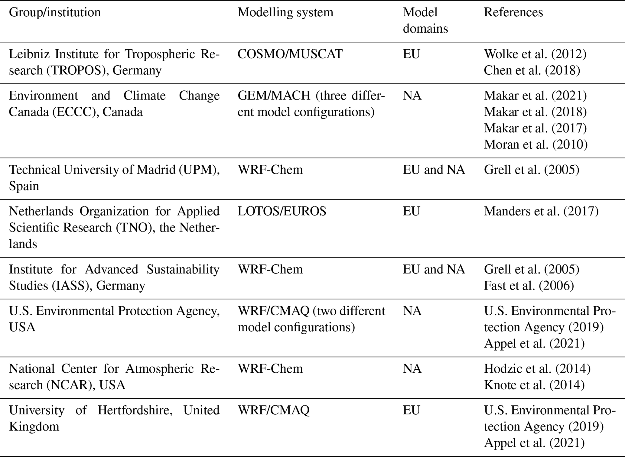
Specifically, the years of interest in AQMEII4 are North America – 2010 and 2016 and Europe – 2009 and 2010. The NA years were selected due to their policy relevance; the years 2010 and 2016 have featured in policy-relevant emissions scenario simulations by governments on the continent. In the case of Europe, the years illustrated a marked difference in meteorological signatures between the 2 years, hence providing a gauge of the impact of meteorological variability on deposition. Modelling multiple years also allows the investigation of the variability of impacts of emission policies and weather conditions on deposition patterns.
All modelling groups carried out simulations on their own grid projections. These “native grid” simulations were interpolated to a common latitude–longitude (Fig. 1) grid over each continent to allow direct comparison of gridded model data:
-
NA: 23.5∘ N ↔ 58.5∘ N, 130∘ W ↔ 59.5∘ W,
-
EU: 25∘ N ↔ 70∘ N, 30∘ W ↔ 60∘ E.
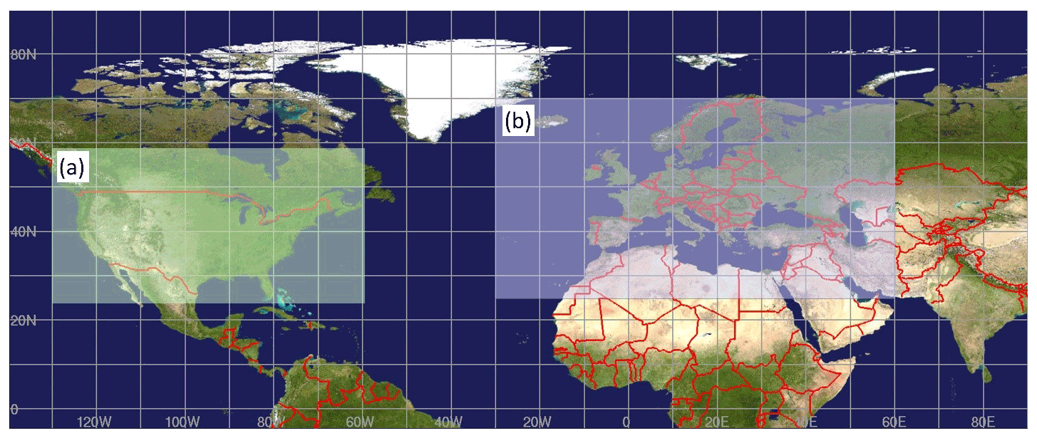
Figure 1AQMEII4 North American (a) and European (b) 0.125∘ grid cell size common latitude–longitude comparison domains.
Modelling groups are expected to perform their simulations on a grid with comparable to higher horizontal resolution as these reported grids. For the interpolation of model results from the native modelling grid to the common analysis grid, a mass-conserving method was recommended for concentrations and fluxes, and the nearest-neighbour method was recommended for diagnostic variables.
2.2 Model inputs shared by all participants
Air quality models require input fields for meteorology, emissions, and chemical boundary conditions; differences in each of these fields lead to differences in model results. All AQMEII exercises have considered the driving meteorology to be an integral part of each participating model (for on-line models, such as studied under AQMEII-2, chemistry and meteorology are inseparable, since both are included in the same modelling platform) and have therefore not attempted to harmonize meteorological fields across participants. However, variations caused by different emissions and chemical boundary conditions are removed in all AQMEII phases by requiring all participating models to use a common set of emissions and lateral chemical boundary conditions (Galmarini et al., 2012, 2015, 2017). Note that due to their dependence on model-specific LULC and meteorology, biogenic emissions are not prescribed and are generated by each group. For AQMEII4, the common model inputs were prepared as follows.
2.2.1 Anthropogenic emissions
Emissions for anthropogenic sources over NA were prepared from US, Canadian, and Mexican inventory data using the emissions processing approach developed for U.S. EPA “emission modelling platforms” (EMPs). An EMP includes not only the underlying point source, county, or province level inventory data but also controls the temporal and spatial allocation and chemical speciation of these inventories. For 2010, the processing was based on the “2011v6.3 EMP” (https://www.epa.gov/air-emissions-modeling/2011-version-63-platform, last access: 7 October 2021). Year-specific adjustments for 2010 were made to the EMP for several sectors (e.g. electric generating units, mobile sources, and residential wood combustion), and Canadian emissions were based on a 2010 inventory rather than the 2013 inventory projected to 2011 used in the EMP. For 2016, the processing was based on the “2016beta EMP” (https://www.epa.gov/air-emissions-modeling/2016v72-beta-and-regional-haze-platform, last access: 7 October 2021), which is documented at http://views.cira.colostate.edu/wiki/wiki/10197, last access: 7 October 2021. These EMPs were used by the U.S. EPA to generate eight different hourly files of speciated emissions for each day in 2010 (one gridded file with low-level emissions and files with elevated sources from seven different sectors) and nine different hourly speciated files for each day in 2016 (one gridded file with low-level emissions and files with elevated sources from eight different sectors), which were then shared with all participants. Speciation was performed for both the CB6R3 and SAPRC07 mechanisms to provide flexibility to participants to map emissions to the chemical mechanism used in their model. The same data were used by Environment and Climate Change Canada to generate day-specific emissions for the GEM-MACH air quality model, for the ADOMII mechanism used within that model. Annual gridded anthropogenic emissions using the Standard Nomenclature for Air Pollution (SNAP) sector classification scheme were prepared over EU by TNO for 2009 and 2010 as part of the MACC-III project (Kuenen et al., 2015) and were provided to EU modelling groups along with reference temporal allocation and speciation profiles. If necessary, EU modelling groups used other emission datasets available to them to fill in emissions near the edges of their modelling domains if their modelling domains extended beyond the area covered by the MACC-III emissions provided by TNO.
2.2.2 Forest fire emissions
The forest fire emissions over NA for 2010 were a combination of emissions over the US included in the “2011v6.3” EMP and emissions over Canada provided by Environment and Climate Change Canada (ECCC; Chen et al., 2013) while 2016 forest fire emissions over both the US and Canada were obtained from the “2016 beta” EMP. Data distributed to modelling groups included both the mass of emissions of criteria air contaminants (speciated into the gases of the gas-phase chemistry mechanisms noted above) and the parameters necessary to compute plume rise using a prescribed plume rise algorithm based on the large stack plume rise formula of Briggs (Briggs, 1971, 1972). While different modelling platforms often have their own approaches for estimating forest fire emissions, particularly in an operational context, as was the case for anthropogenic emissions, this unified approach was adopted in order to reduce the variability in model performance associated with emissions inputs. Forest fire emissions for 2009 and 2010 over EU were provided by the Finnish Meteorological Institute and were developed using the IS4FIRESv2 methodology described in Soares et al. (2015). These emissions were vertically allocated to eight layers with heights ranging from 50 to 6200 m, with individual groups re-allocating the resulting mass to their own vertical discretization.
2.2.3 NO emissions from lightning
Although previous phases of AQMEII did not consider NO emissions from lightning, these emissions were included in the current phase due to their impact on nitrogen deposition fluxes. To provide a unified forcing from this source across all models, the emissions were based on the GEIA monthly climatology (Price et al., 1997) rather than in-line parameterizations based on meteorological fields implemented in some but not all participating models. Although using climatological lightning does not capture the linkage between modelled meteorology and NO emission from lightning, this approach ensures that the bulk effects are included in all modelling systems and streamlines the interpretation of the modelling results by removing a potential difference in emissions input. The monthly climatological values were allocated diurnally based on Table 2 in Blakeslee et al. (2014) and distributed to participating groups as two-dimensional files. Groups were then asked to allocate these emissions to their specific vertical grid based on Table 2 of Ott et al. (2010), using the tropical profiles for land and water (or an average of the two) for grid cells with latitudes below 23.5∘ N, the subtropical profile for grid cells with latitudes between 23.5 and 40∘ N, and the mid-latitude profile for grid cells with latitudes >40∘ N.
2.2.4 Chemical boundary conditions
Concentrations of the 33 longer-lived trace gas and aerosol species listed in Table 2 were provided by the European Centre for Medium-Range Weather Forecasts (ECMWF) for the two continents and for the modelled time periods so that participants could prepare initial and boundary conditions for their regional-scale modelling domains. The concentration fields were based on the Copernicus Atmospheric Monitoring Service (CAMS) EAC4 reanalysis product (Inness et al., 2019) and were provided every 3 h on a grid with 54 vertical levels from the surface to 2 hPa. The vertical grid structure varied in both resolution and vertical extent across models, and individual participants were responsible for interpolating the CAMS fields to their horizontal and vertical grid structure. The CAMS species were matched by participants to their own internal model speciation (and, in the case of the particulate matter emissions, to the particle size distribution of their own models).
Table 2Variables from the CAMS EAC4 reanalysis provided for the generation of initial and boundary conditions.

* Based on guidance from ECMWF, participants were advised to transform the provided values back to dry matter by applying a reduction factor of 4.3 for the mass mixing ratios and a reduction factor of 1.99 for the radii of the sea salt bin limits.
2.3 Standard model outputs
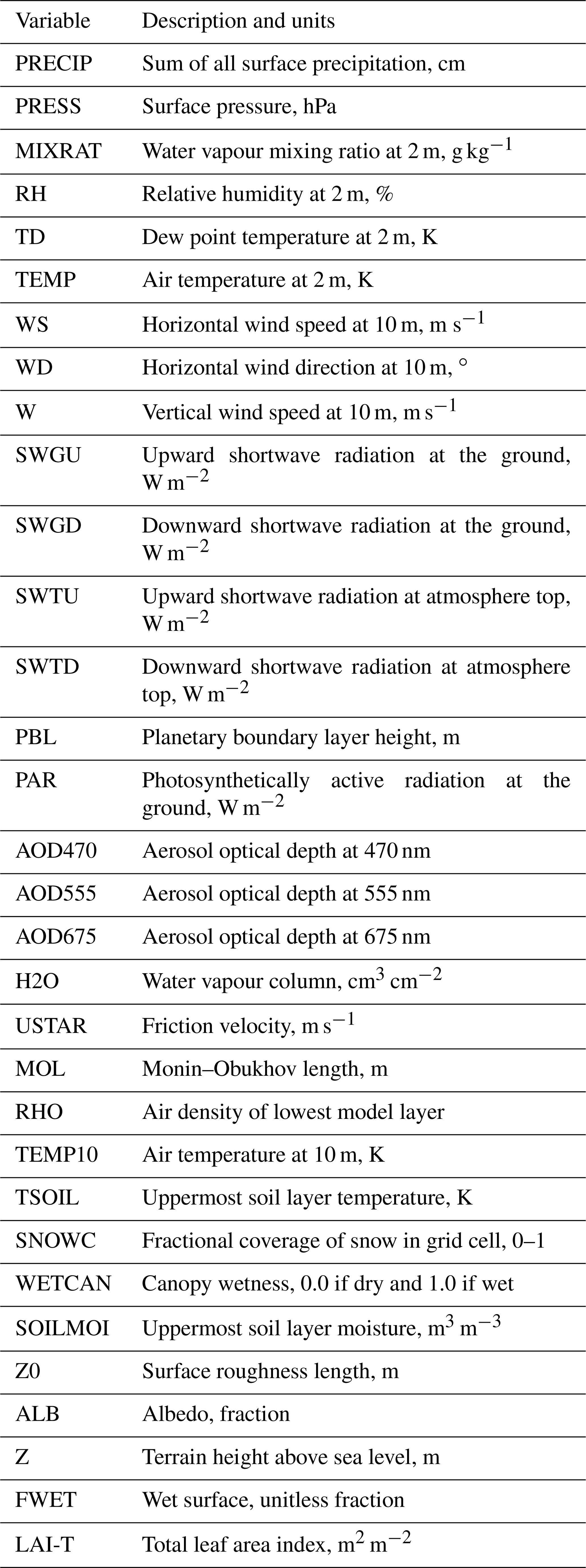
We distinguish here between model output similar in scope and intent to previous ensemble model comparisons in past phases of AQMEII (i.e. “standard model outputs”) and the detailed diagnostic outputs reported under AQMEII4. The standard output requested from all participating models comes in two major forms: as hourly gridded surface concentrations and meteorological variables on the common grids described earlier and as model values extracted at monitoring network station locations. Tables A1–A3 of Appendix A list the variables requested for gas- and particle-phase species, meteorology, and grid-scale deposition fluxes. The meteorological variables have been extended considerably compared to past phases of AQMEII, to include more parameters that describe the planetary boundary layer. The gridded fields of integrated emissions were also requested as output, to be used to check that the right amounts of masses were inputted into the models.
A list of all available surface monitoring locations in both continents for concentrations of gas- and particle-phase species, precipitation chemistry, and meteorology was distributed to the AQMEII4 participants who are expected to produce model results for all species presented in Appendix A for the grid location closest to the monitor or interpolated to the monitoring. In particular, we note that the analysis of wet deposition in AQMEII4 will rely on the precipitation and wet deposition flux variables listed in Table A3. Note that the units of nitrogen and sulfur deposition in Table A3 are “equivalents” per hectare per year, where the equivalent refers to the product of moles and the oxidized charge associated with the deposited species. All species depositing sulfur are assumed to have a charge of 2, and all species depositing nitrogen we assumed to have a charge of 1. These units are used in the calculation of exceedances of critical loads, where the annual charge balance and flux of charge to ecosystems is used to estimate potential ecosystem impacts. For more information on the routine monitoring networks used in AQMEII, please refer to Galmarini et al. (2012, 2015, 2017).
Analysis of dry deposition is the focus of AQMEII4. In particular, AQMEII4 intends to go beyond an operational evaluation of ambient concentrations and comparison of total deposition across models because this approach does not provide enough information to determine the causes of different deposition totals among regional models. The novelty of AQMEII4 is that we request additional and very detailed diagnostic-evaluation outputs related to dry depositional from all of the models. With these very detailed outputs, we can compare the important elements of the model machinery and understand model differences.
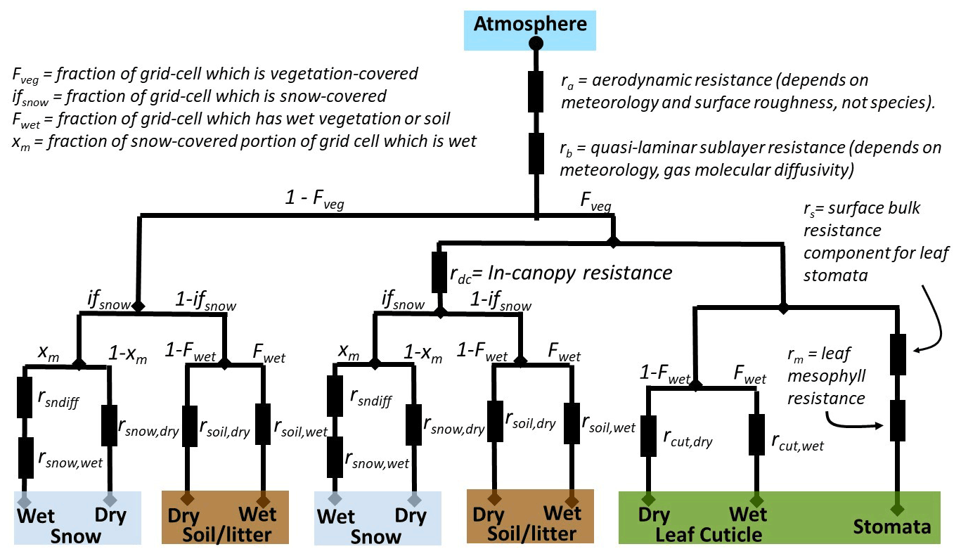
Many regional models use the Wesely (1989) dry deposition scheme, but several variants have been developed and implemented with different levels of sophistication. Dry deposition schemes are mostly resistance frameworks – by framework, we mean the structure of the scheme with respect to how processes relate to one another – and all of the regional models in AQMEII4 use resistance frameworks for dry deposition. Resistance frameworks are based on the representation of series and parallel resistors in electrical circuits. Differences in resistance frameworks across regional models imply that comparing a given process among the regional models is not straightforward. Thus, diagnostic variables that account for differences in resistance frameworks need to be reported. Below, we present the strategy devised to reduce any dry deposition scheme to the essential set of comparable variables regardless of the differences in the frameworks of the schemes that generated them.
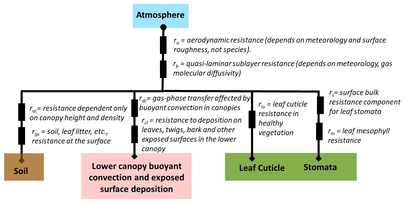
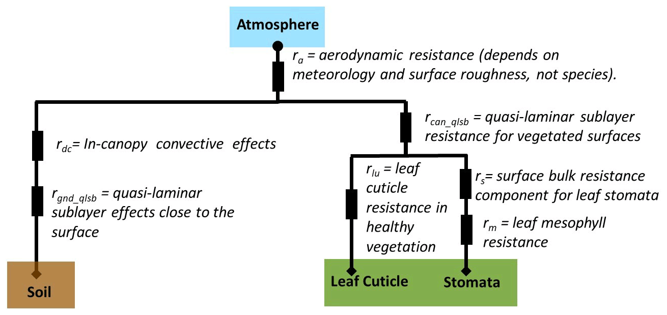
Figure 2Schematic of the resistance framework for gas-phase dry deposition for the Wesely (1989) scheme. Circles and diamonds show where ozone concentration is needed as input for a given framework. At the diamonds, the ozone concentration is assumed to be zero. Rectangles indicate resistances.
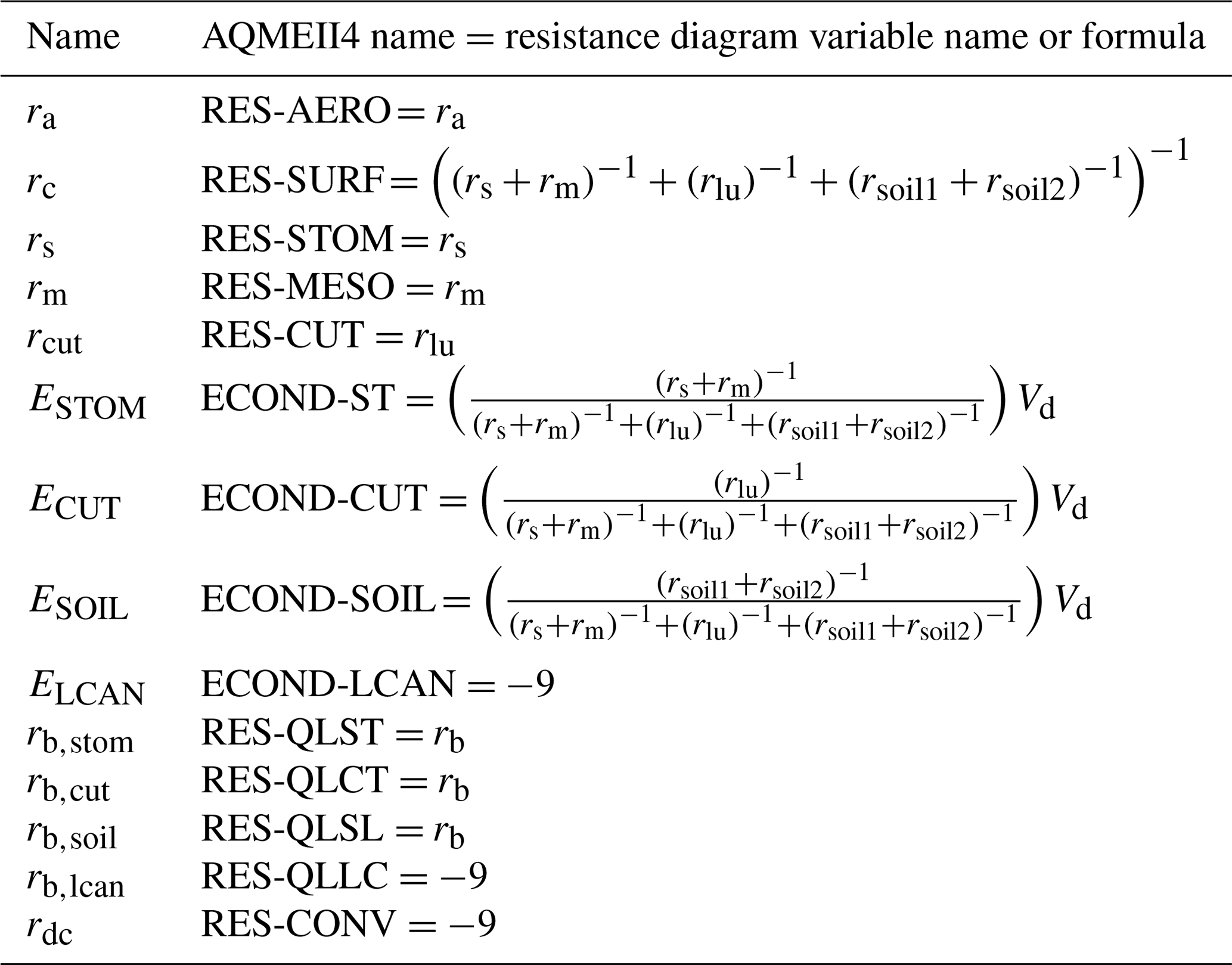
We start with a description of the Wesely (1989) resistance framework, one of the earliest literature examples of a resistance framework for dry deposition and arguably the most popular dry deposition scheme, and follow with both generic and specific examples of other resistance frameworks as a guide to the AQMEII4 output protocol. The components of the deposition velocity are process-based resistances (units are s cm−1) that impede the transfer of mass to a variety of surfaces. Resistances are added in series for processes operating on the same depositional pathway, and in parallel when multiple surfaces for dry deposition exist. In the original Wesely (1989) scheme, four deposition pathways were used: soil, “lower canopy and exposed surfaces”, leaf cuticles, and plant stomata. Gases are first impeded by an aerodynamic resistance to deposition (ra), second impeded by a quasi-laminar sublayer resistance (rb), and third impeded by a bulk surface resistance term (rc) composed of a parallel summation of the resistances associated with each pathway. The three impedances to deposition are added into a total resistance, the inverse of which is the deposition velocity of the gas (units = cm s−1):
The bulk surface resistance (rc) in Wesely (1989) follows
The component resistances used in rc are defined in Fig. 2, which is a schematic of the Wesely (1989) resistance framework.
Work subsequent to Wesely (1989) also uses the resistance approach, but sometimes with considerable variation in the resistance framework, the number of surfaces to which dry deposition occurs, and/or the processes represented by individual resistances. Several motivating factors likely led to the development of a diversity of resistance frameworks. In the intervening years subsequent to Wesely's introduction of the resistance framework concept, new measurement capabilities (for higher-time-resolution information, for greater chemical speciation, higher-precision measurements) allowed the original algorithms to be tested and modified. Developments in plant physiology understanding have also resulted in improved stomatal resistance parameterizations. Examples include the observation-based introduction of bidirectional fluxes for ammonia gas and improved understanding of the role of CO2 fluxes in the deposition of other gases. Also, some divergence in approaches is likely due to algorithm developments having been made in the context of specific regional models – each of which encompasses a diverse range of process representation algorithms, vertical resolutions, horizontal resolutions, etc. An algorithm which provided good performance relative to surface concentration observations within the context of one regional model thus may not have resulted in as good of performance in another model, further spurring model-specific development. These factors have resulted in the variety of approaches for gas-phase deposition in current regional models and provide the part of the motivation for this first attempt at cross-comparing the results of the models' deposition algorithms in detail – to show and explain the causes for these differences.
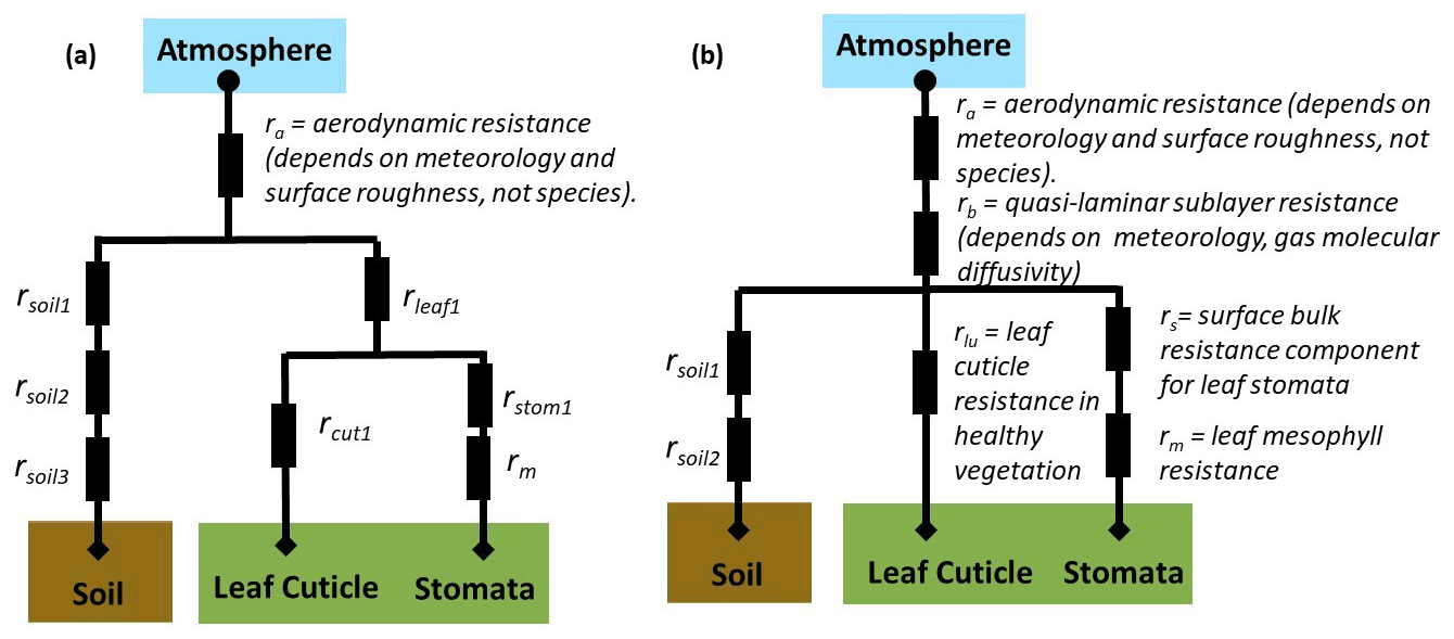
Schematics of resistance frameworks as two generic examples are shown in Fig. 3. In these examples, the Wesely (1989) deposition pathway for “lower canopy buoyancy and exposed surfaces” deposition is not included. The example of Fig. 3a also lacks a quasi-laminar sublayer resistance rb applied across all surface types. Instead, surface-specific quasi-laminar sublayer resistances are used: rsoil2 for soil and rleaf1 for leaves. The examples in Fig. 3 demonstrate two ways in which the resistance framework has been adapted from Wesely (1989). In general, the diversity in resistance frameworks across models complicates model intercomparison of individual resistances.
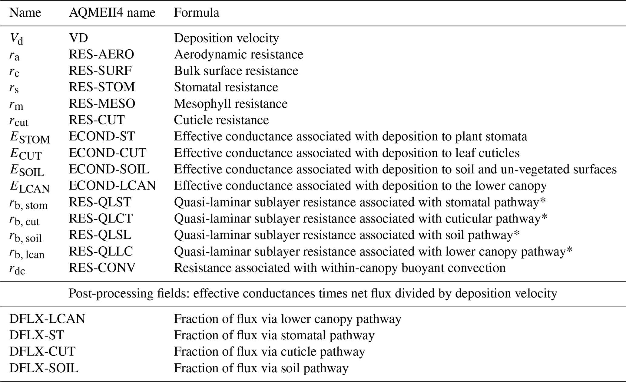
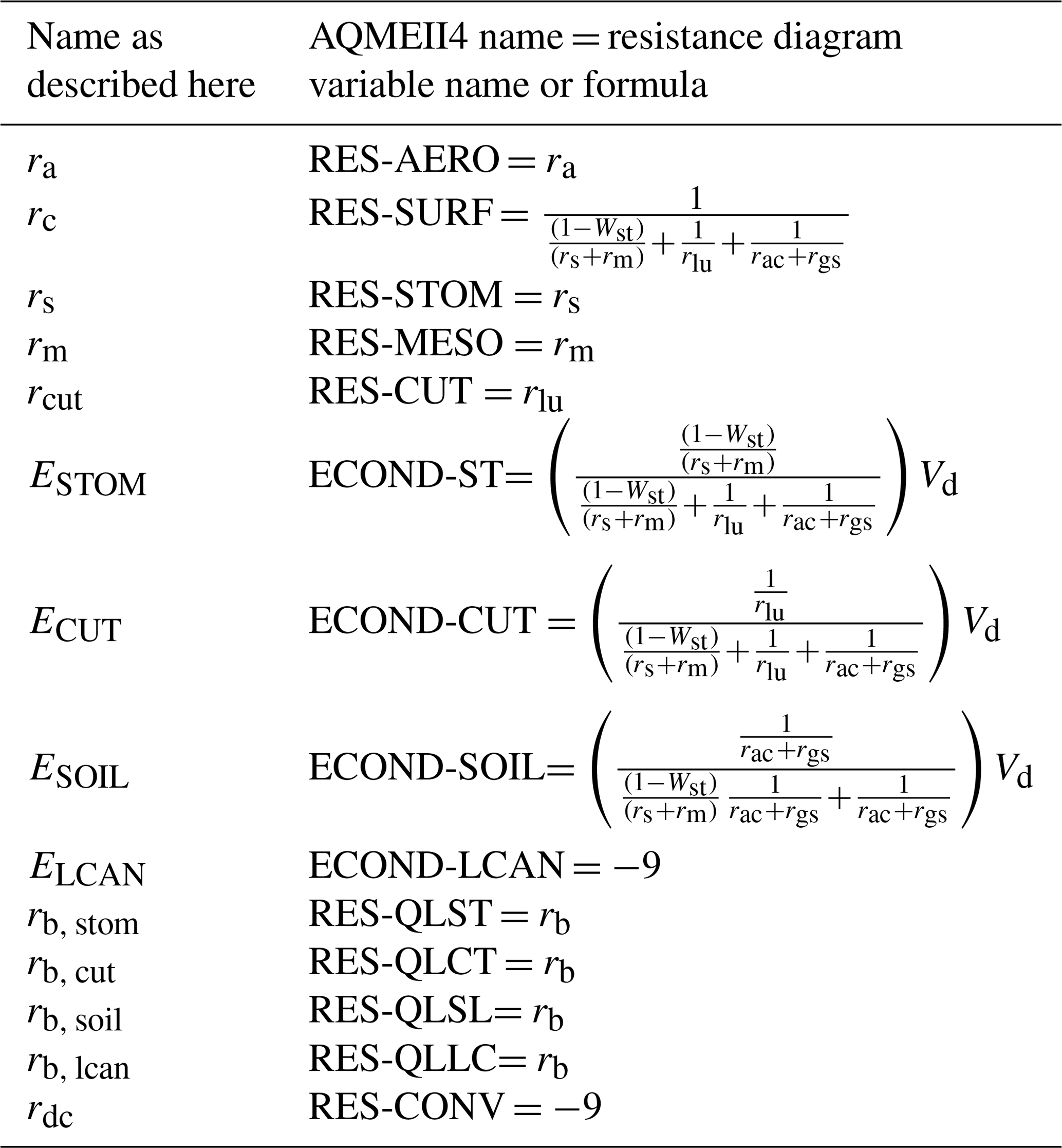
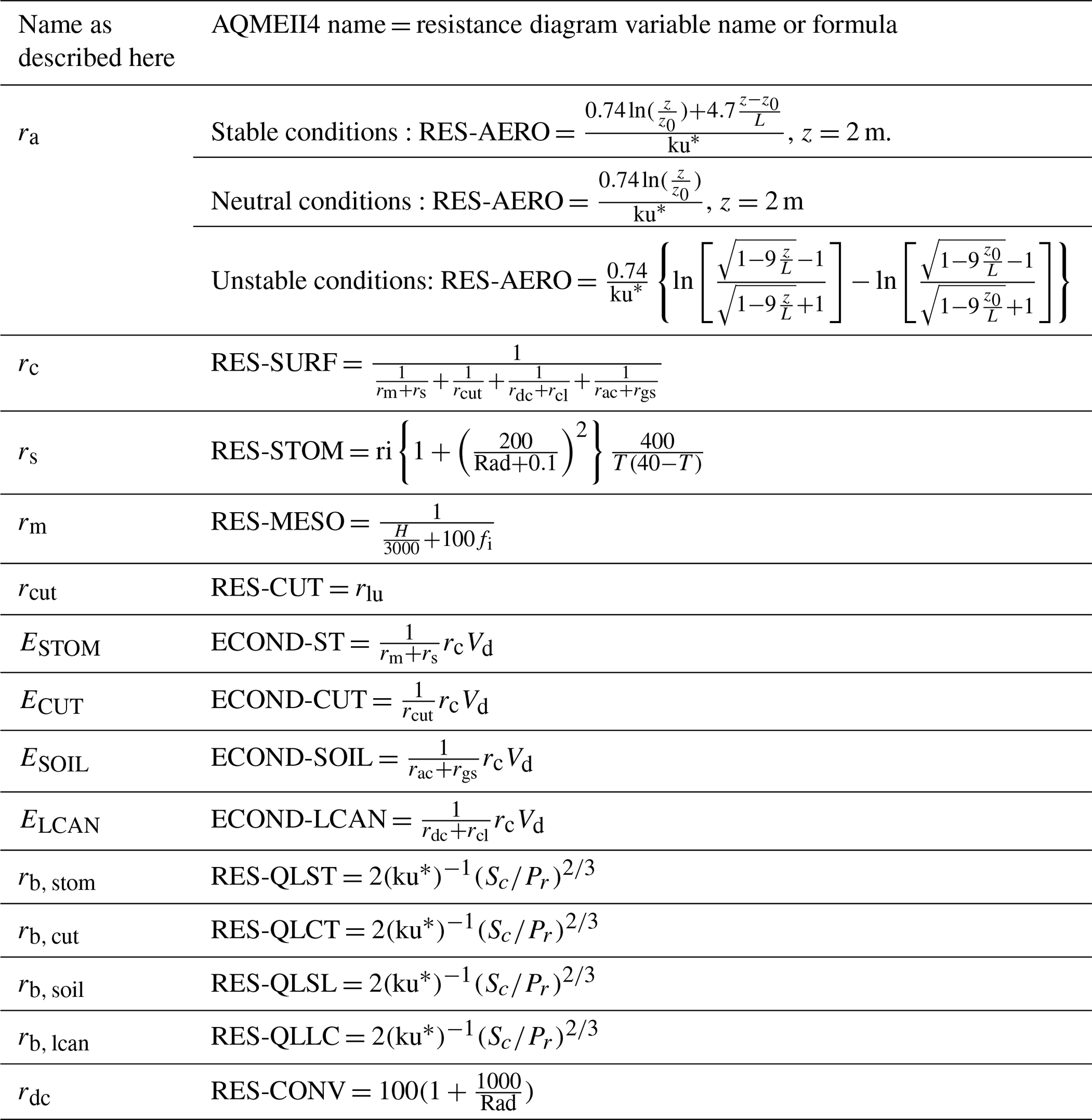
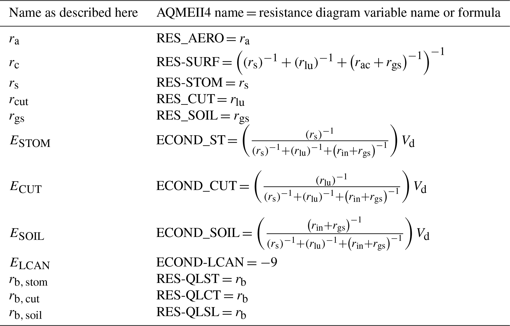
When there are differences in resistance frameworks across models, the deposition pathways may be compared across models using a construct we will refer to here as effective conductance (Paulot et al., 2018; Clifton et al., 2020b). While generally a conductance is simply the inverse of a resistance, an effective conductance is the contribution of a given depositional pathway to the deposition velocity, expressed in the same units as the deposition velocity. The sum of the effective conductances for all deposition pathways is the deposition velocity. The effective conductances of the soil (ESOIL), lower canopy (ELCAN), cuticle (ECUT), and stomata (ESTOM) branches specifically for Wesely (1989) are given by1:
The denominator in each of Eqs. (3) to (6) is the inverse of the bulk surface resistance rc and the numerators are the inverses of the resistances associated with each pathway in rc. We emphasize that the calculation of the effective conductances depends on the resistance framework used; Eqs. (3) to (6) are specific to Wesely (1989) and require modification for other resistance frameworks, and we provide examples of formulae for these terms for other frameworks, in Sect. 4.1 and Appendix B. Calculation of the effective conductances requires either archiving all component resistances in a given framework and subsequent post-processing or their online calculation.
For any given model, effective conductances are an invaluable tool for determining the extent to which each pathway impacts dry deposition velocity, and which deposition pathways drive spatiotemporal variability in dry deposition velocity. Key for AQMEII4, the effective conductances allow a cross-comparison of the main deposition pathways across different resistance frameworks. The primary terms of comparison for dry deposition schemes in AQMEII4 are thus the effective conductances. In addition, given that many models' resistance frameworks follow Wesely (1989), we also request those individual resistance terms held in common by most models to allow exact comparisons of individual processes which may influence or control a given pathway. These resistances include
-
a term for the aerodynamic resistance, ra;
-
a term for the bulk resistance to deposition associated with surfaces, rc;
-
a term or series addition set of terms describing the stomatal resistance, rs;
-
a term or series addition set of terms describing the mesophyll resistance, rm;
-
a term or series addition set of terms describing the cuticle resistance, rc;
-
terms to describe quasi-laminar sublayer resistance, rb;
-
a term to describe within-canopy buoyant convection, rdc.
With regards to (6), the implementation of quasi-laminar sublayer resistance (rb in Wesely, 1989) tends to differ among models. Some models use the Wesely (1989) concept of a pathway-independent quasi-laminar sublayer resistance. Others use quasi-laminar sublayer resistances as pathway-dependent (e.g. Fig. 2a, where the rsoil2 and rleaf1 represent quasi-laminar sublayer resistances for soil and leaf pathways, respectively). The quasi-laminar sublayer resistance is thus reported in AQMEII4 for each pathway, with the models for which the term is independent of pathway reporting the same value for each pathway. Pathway-dependent quasi-laminar sublayer resistances are to be reported as “not present” only if the given pathway does not exist in the framework.
Note that models that include a single deposition pathway to soil that incorporates rdc are requested to report that pathway as “lower canopy” not “soil”. For example, the LOTOS-EUROS dry deposition scheme (Fig. B4) reports the effective conductance calculated for the soil pathway as ELCAN due to the presence of the in-canopy resistance term in this pathway. In contrast, the CMAQ-M3DRY and CMAQ-STAGE dry deposition schemes (Figs. B2 and B3) have two separate pathways for deposition to soil, one for vegetation-covered soil and one for bare soil. Due to the inclusion of the in-canopy convective resistance in the computations for vegetation-covered soil, the effective conductance for that pathway is reported as ELCAN, while the effective conductance for the bare soil pathway should be reported as ESOIL.
Specific resistance terms for the soil deposition pathway and the lower canopy pathway have not been requested because the resistance frameworks for these pathways vary considerably across models, and therefore specific resistance terms are not easily comparable. For example, Wesely (1989) used a single term for the soil resistance (Fig. 1) while other models may use two or three resistances related to dry deposition to soil only and added in series (Fig. 2).
In addition to the effective conductances, another set of diagnostic fields is calculated during post processing: the time-aggregated fractional mass (or charge equivalent) flux transferred to the surface via each of the four deposition pathways (hereinafter, effective flux). The effective flux is calculated on an hourly basis prior to conversion to AQMEII4 time-aggregated gridded and station data using ENFORM and is the product of the hourly effective conductances, dry deposition mass fluxes, and inverses of the deposition velocity. Effective conductances provide an estimate of the importance of each pathway towards the deposition velocity. However, since the flux depends on the deposition velocity and the near-surface air concentration, which both vary on hourly timescales, estimating the aggregate importance of each deposition pathway towards the flux requires calculating the effective flux before time aggregation.
Figure 4 provides an example of the different yet complementary information resulting from effective conductances and effective fluxes, showing hourly SO2 concentrations, effective conductances, and effective fluxes for a boreal forest impacted by a large industrial SO2 stack source and hourly NO2 concentrations, effective conductances, and effective fluxes for a location to the north-east of New York City. In both cases, high concentrations of the pollutant gas (Fig. 4a, d) occur at night, while the deposition velocity, due to the stomatal pathway (Fig. 4b, e), maximizes during the day. As a result of the low daytime concentrations, the effective fluxes for SO2 (Fig. 4c) show a relatively minor contribution of the stomatal pathway to the deposited mass despite the major contribution of the stomatal pathway to the daytime deposition velocity. As the result of high night and morning concentrations, the effective fluxes for NO2 (Fig. 4f) show separate day and night peaks of about equal magnitude, with the stomatal pathway dominating daytime values and roughly equivalent contributions from stomatal and soil pathways at night.
Also with reference to Fig. 4, it should be noted that the effective conductances and effective fluxes show the relative contributions of the pathway towards the total deposition or the total flux at any given time. It should also be noted that the net surface resistance appearing in the denominator of these terms may drive the time variation. For example, the soil effective conductance of Fig. 4e minimizes at 6:00 LT – however, the factors contributing to the soil pathway itself for the model used in this example (see Appendix Table B1) are relatively time-invariant (seasonally varying). The temporal variation is driven by hourly variation in the stomatal term and hence the relative importance of the soil conductance varies with time in Fig. 4e.
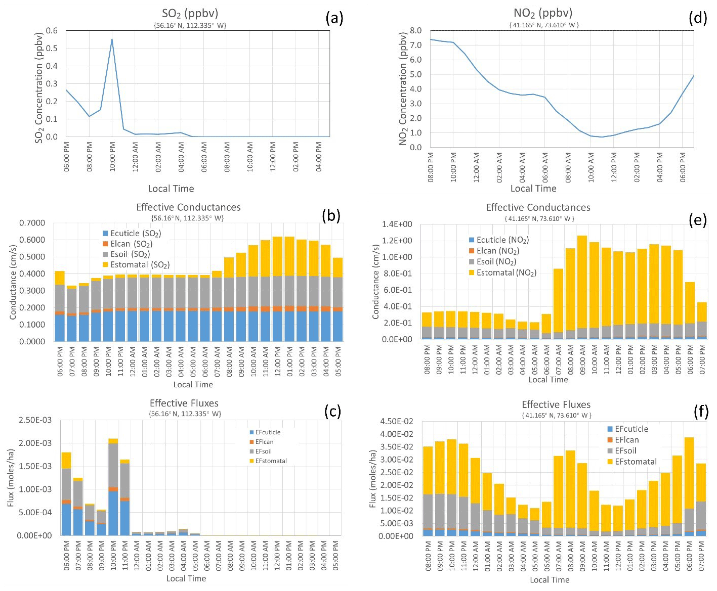
Figure 4Two examples of diurnal variations in concentrations (a, d), effective conductances (b, e), and effective fluxes (c, f) for SO2 (left column) and NO2 (right column).
We also consider that dry deposition strongly depends on LULC type, and different models use unique LULC databases. We thus request LULC-specific variables along with the fractional areal coverage for each LULC type, which allows quantification of not only the impacts of different LULC-specific processes and parameters on dry deposition, but also the impacts of different LULC databases. “Generic” AQMEII4 LULC types were devised due to the use of a wide variety of LULC databases across air quality models, in terms of both the source of the data and the number of LULC types employed. The AQMEII4 LULC types listed in Table 2 are broad LULC types into which the model-specific LULC types could be aggregated, to allow intercomparison between models. Study participants aggregated their LULC-model-specific diagnostic outputs to the set of common AQMEII4 LULC types using the fractional representation of each native LULC type contributing to the AQMEII4 type within each grid cell. Generic AQMEII4 LULC types were constructed after analysis of the LULC schemes in the participating models. A suggested mapping between model and AQMEII4 LULC types was provided to participants, along with the instruction that the mapping actually employed should be reported. The grid cell fractions of both the native model LULC types and the resulting fractions of AQMEII4 LULC types were reported by participants. Note that there is a large variety in number and therefore types of LULC across models, and thus each of the generic types represents a rather broad range of LULCs.
We also note that the mapping of LULC types from the individual model land use classifications to the AQMEII4 land use classifications is an unavoidable source of uncertainty in the land-use specific diagnostics. The 15 AQMEII4 land use types themselves were based on a survey of land-use classifications used in 17 regional models. For example, while “Herbaceous” is available as an AQMEII4 land use category, its intent is for use for moors and heathlands, while AQMEII4 land use category “Wetlands” encompasses wetlands which are diversely described in individual model land use categories such as herbaceous, wooded, and permanent wetlands, as well as swamps and peatbogs. However, some categories were included most models (e.g. evergreen needleleaf forest, deciduous broadleaf forest, snow and ice, mixed forest, usually taken as a combination of needleleaf and deciduous forests), while others could easily be classified according to the broader landscape type of which they were a member (e.g. different types of tundra were recommended to be classified as the AQMEII4 Tundra classification). Both the AQMEII4 and “native model” land use types were reported by participants – with the aim of using both sets of information to determine the extent to which land use database variation may be a factor in estimating deposition velocities and to provide information on specific land use types used by specific models when these differences appear to be large.
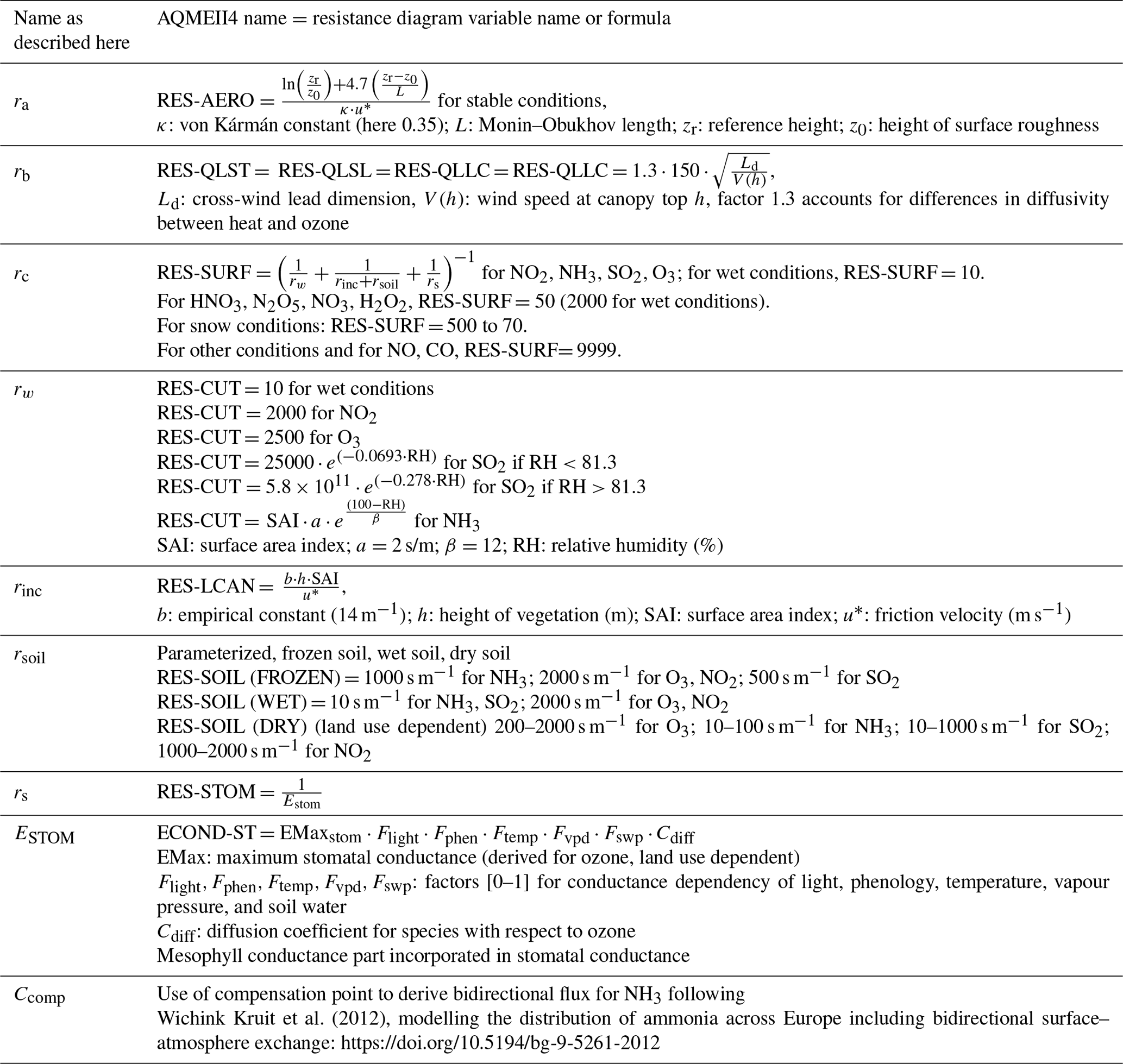
For AQMEII4, the terms listed in Table 4 were reported for SO2, NO2, NO, HNO3, NH3, PAN, HNO4, N2O5, organic nitrates, O3, H2O2, and HCHO, both as a function of the 16 generic AQMEII4 LULC types (Table 3) and for the net grid-scale calculation for each grid cell and/or receptor. Models employing bidirectional flux algorithms for the dry deposition of atmospheric NH3 reported a different set of terms, given in Sect. 4.2.
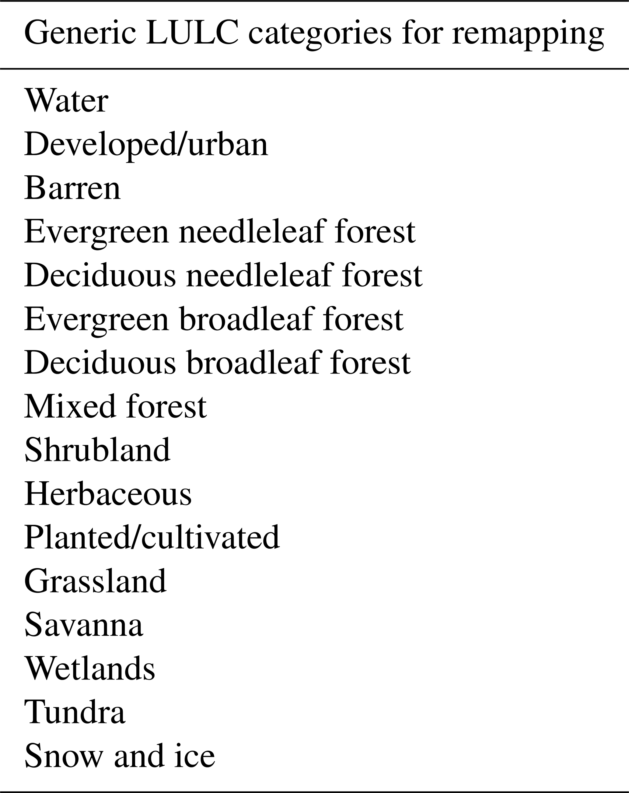
Table 4 summarizes the diagnostic variables related to gaseous dry deposition reported by all participants, the variable names as described in the AQMEII4 technical specification documents (TSDs), and a description of each variable. Equations (2) through (6) and the related text describe the terms specifically for the resistance framework of Wesely (1989); additional examples for participating models' resistance frameworks are provided in the Appendix tables and figures.
The presence of surface wetness or snow is incorporated into the effective conductance, effective flux, and component resistances. In other words, separate component resistances or effective conductances and fluxes for snow-covered or wet surfaces were not reported. In order to compare the impacts of the different models' predictions regarding snow cover or wetness, additional diagnostic variables were requested to describe surface state (e.g. fractional snow cover and either the values of binary wet–dry conditions or fractions in surface wetness).
Table 4AQMEII4 reported dry deposition diagnostic variables for gas-phase species.
* Equal to rb if this is pathway-independent for the resistance framework.
Gridded dry deposition diagnostic variables were archived as hourly values for the native LULC types and then converted to the generic AQMEII4 LULC types during post-processing. The ENFORM Fortran code provided to all participants was used to convert gridded fields from the hourly values to temporal aggregations of the hourly values. Hourly diagnostics were converted to “monthly median diurnal” values using ENFORM by taking the medians of all values for a given UTC hour in a given month, thus reducing 8760 hourly values for each year to 288 values (24 h × 12 months). The use of monthly median diurnal values is motivated by the need to reduce the amount of data to be transferred and analysed on a single server (despite this aggregation, each year of gridded model output requires up to 200 Gb of storage), while preserving the key aspects of diurnal and seasonal variations.
The use of a median rather than an arithmetic mean for AQMEII4 diagnostic time aggregation resulted from consideration of the manner in which different dry deposition algorithms deal with pathways that effectively shut down under certain conditions. For example, some algorithms employ an upper-limit resistance to represent conditions under which the pathway transmits little mass to the surface (e.g. nighttime stomatal resistances may be set to very large values). Others simply use code branching to prevent a pathway from contributing to rc (e.g. the entire stomatal pathway is removed from rc at night). Others employ different resistance frameworks for different conditions (e.g. to account for snow-covered surfaces). However, the AQMEII4 protocol requires participants to submit “missing values” as a specific code (−9) in order to allow filtering of valid from invalid data during time aggregation. An algorithm removing a pathway may thus have a different number of valid values from an algorithm employing a large resistance. Similarly, a seasonal transition where the resistance network changes depending on whether a surface is snow-covered becomes difficult to interpret in a time average, whereas valid time-median values allow for a more meaningful comparison.
Table 5AQMEII4 dry deposition diagnostic variables for gas-phase species corresponding to the resistance framework of Fig. 2a.
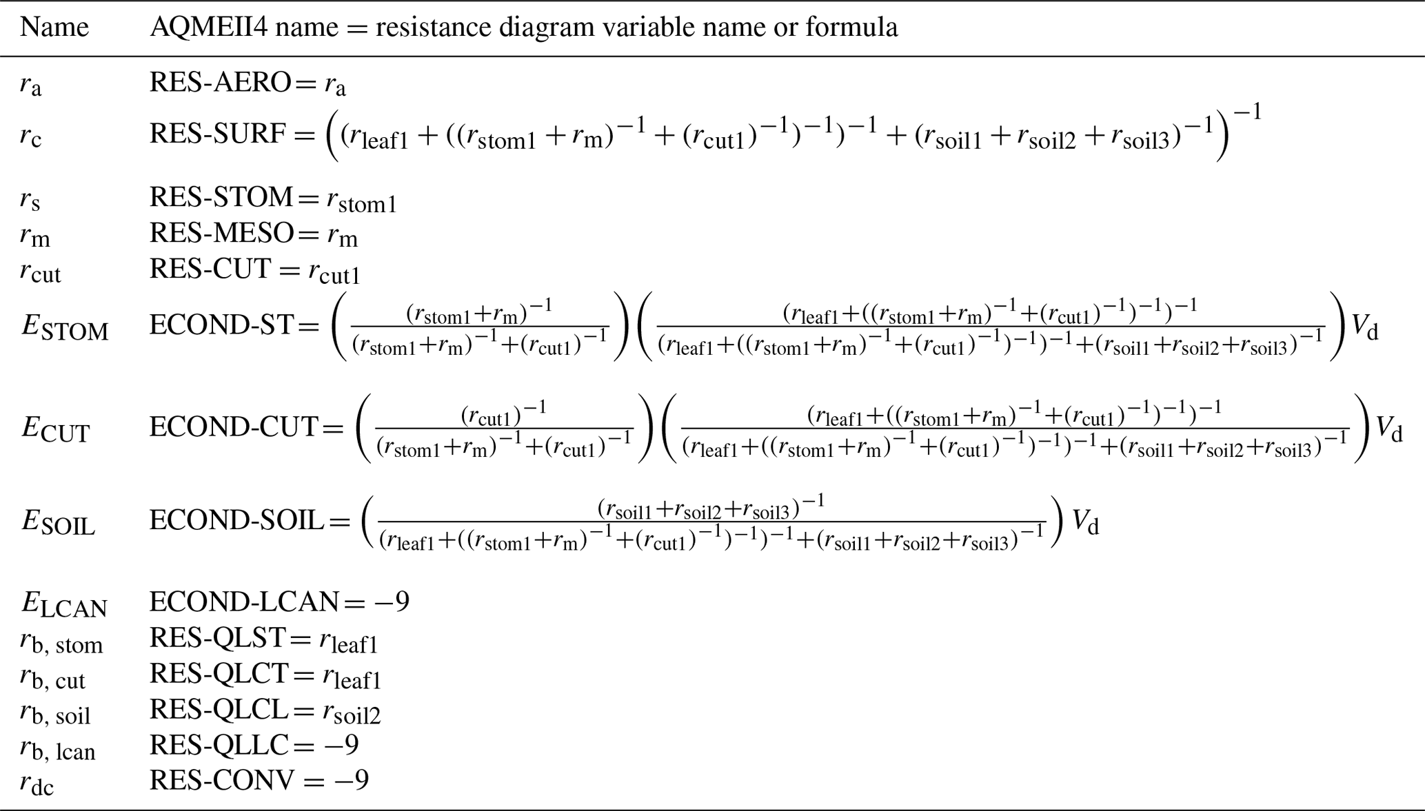
Table 6AQMEII4 dry deposition diagnostic variables for gas-phase species corresponding to the resistance framework of Fig. 2b.
For example, if only 20 % of the resistances at 14:00 LT in a given month and grid cell are snow covered, then the monthly median for 14:00 LT would represent values typical of snow-free conditions, for both models representing resistances under snow-covered conditions as missing and models representing them as large values. Thus, the monthly median comparison represents the most common conditions encountered during the month for both models. On the other hand, while the monthly average resistance for 14:00 LT represents snow-free conditions for the model that treats snow-covered hours as missing, the monthly average for the model that represents snow-covered conditions as a large value is not meaningful and complicates inter-model comparison.
Monthly median diurnal values capture both seasonal and diurnal variations in the archived fields and allow comparisons between algorithms shutting off a pathway by removing the pathway and algorithms shutting off a pathway with high resistance values. Note that the same data completeness criterion used for comparing simulated and observed ambient concentrations was employed here for the construction of the median values. Specifically, more than 75 % of the values within a month were required for a median to be constructed.
4.1 Variations on the Wesely (1989) resistance framework
For the sake of clarity, we provide examples of how specific dry deposition schemes can be reduced to the common set of variables described above. The generic schemes presented in Fig. 2a, b along with the Nemitz et al. (2001) bidirectional scheme for NH3 have been selected as examples here, while Appendix B provides additional examples for specific schemes implemented in participating models. The AQMEII4 protocol and these specific examples provide a standard form of representing key aspects of dry deposition schemes, which may be adopted by similar activities or initiatives in the future. Note that some of these example algorithms do not have a separate resistance for lower canopy buoyant convection or a deposition pathway to the lower canopy and exposed surfaces; hence the associated effective conductance (ECOND-LCAN) and resistance (RES-CONV and RES-QLLC) terms are not reported.
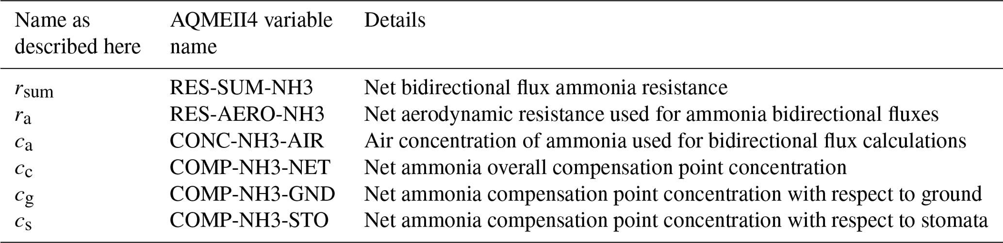
4.2 Bidirectional fluxes of ammonia – a special case
Some models make use of the concepts of bidirectional fluxes when describing ammonia gas transfer from and to surfaces. In the bidirectional flux paradigm, the difference between the ambient gas concentrations and near-surface (compensation point) concentration is used to determine the direction of the flux: if the ambient air concentration is greater than the compensation point concentration, the flux is downward (i.e. deposition occurs) while in the reverse case the flux is upward (i.e. the emission of ammonia previously stored in the surfaces takes place). The algorithms used in the subset of models employing ammonia bidirectional fluxes were examined, in order to determine common terms that could be used for points of comparison across the algorithms. As an example, we present the bidirectional flux model of Nemitz et al. (2001) below (Fig. 5 and Table 7), used within CMAQ to represent bidirectional ammonia gas fluxes. In addition, we also include a comparison of two ammonia bidirectional flux calculations in Appendix C.
The bidirectional flux algorithms were analysed as a separate case, with the result that a revised and smaller number of variables were reported for the specific case of ammonia bidirectional fluxes than for other gases, focusing on the compensation point concentrations as diagnostics for the cross-comparison of these algorithms. The reported variables in this case are ammonia's aerodynamic resistance, its net surface resistance, and three compensation point concentrations, for stomata and ground and net compensation points, respectively. These specific parameters for ammonia bidirectional fluxes appear in Table 7, and a detailed comparison of two representative bidirectional ammonia algorithms is presented in Appendix C.
In this example, note that the branch containing the “soil” term has been designated as the lower canopy pathway, due to the presence of the canopy buoyant convection term rdc (i.e. closest analogy to Wesely's setup is to have the pathway involving deposition to “soil” pathway designated as a “lower canopy” pathway).
The fourth phase of the Air Quality Model International Initiative has been introduced. The focus of this phase is on wet and especially dry deposition. The necessity of tackling this subject in a diagnostic way prompted us to divide the initiative into two activities, one dedicated to the evaluation of the process as described by four-dimensional air quality regional-scale models and the second dealing specifically with evaluating ozone dry deposition calculated by “single-point model” versions of the dry deposition modules used in the regional-scale models with a collection of ozone flux measurements. Here, the organization of Activity 1 has been formally introduced, whereas Activity 2 will be described in separate AQMEII4 special issue publications. In addition to presenting the standard and common input data and the way in which standard output is expected, we also presented the way in which the very diverse representations of dry deposition in participating models have been reduced to a common representation that will facilitate model inter-comparison. The essence of the adopted methodology is the transformation of individual resistances into effective conductances and effective fluxes, which represent the importance of deposition pathways held in common across the models to the total deposition velocity and flux. Resistances held in common across different modelling frameworks were also reported, to allow comparisons at the sub-pathway level, where possible. Thus, regardless of the level of sophistication of the resistance framework, one can meaningfully inter-compare the results produced by different models.


B1 Example 1: GEM-MACH model, default Robichaud scheme
These are the calculations for the Environment and Climate Change Canada model GEM-MACH (Global Environmental Multiscale- Modelling Air-quality and CHemistry). The resistance diagram for this model is shown in Fig. B1. The deposition algorithm closely follows Wesely's original, hence the similarities to Fig. 2. The scheme includes further modifications incorporating parameterizations from Jarvis (1976), Val Martin et al. (2014), and other authors; details and references for this scheme may be found in Makar et al. (2018), Supplement). In GEM-MACH, snow, when present, is treated as a separate land use type.
The main difference between the resistances in Wesely (1989) and the GEM-MACH resistances (aside from formulation details) is the addition of a surface wetness term, (1−Wst), intended to account for the influence of wet surfaces on dry deposition.
Table B1Example 1: AQMEII4-reported gaseous deposition variables corresponding to the GEM-MACH Robichaud resistance model of Fig. B1.

B2 Example 2: CMAQ M3DRY
The second specific air quality model example is the M3DRY algorithm implemented in the U.S. EPA's Community Multiscale Air Quality (CMAQ) model, one of two available dry deposition options in that model. In this particular case, separate branches occur for the vegetated versus non-vegetated fraction within each model grid cell, and further branching resistance pathways take into account the fraction of the grid cell which is wet versus dry and snow-covered versus non-snow-covered. In-canopy convective effects are only calculated for the vegetated fraction.
Table B2AQMEII4-reported gaseous deposition variables corresponding to the CMAQ M3Dry resistance model of Fig. B2.
Note that the vegetated fraction and leaf area index used in the above equations for CMAQ with the M3DRY deposition option are for specific LULC types: the quantities in Table B2 will be reported for each of the 16 generic LULC categories for AQMEII4. Note that the lower canopy pathway has been identified as such due to the presence of the rdc term; i.e. this points to its similarity with Wesely's original lower canopy pathway.
B3 Example 3: CMAQ STAGE
The third specific air quality model example is the algorithm used by the U.S. EPA's Community Multiscale Air Quality (CMAQ) model with the Surface Tiled Aerosol and Gaseous Exchange (STAGE) deposition option. In this particular case, separate branches occur for the vegetated versus non-vegetated fraction for each LULC type within each model grid cell, and further branching resistance pathways take into account the fraction of the grid cell which is wet versus dry and snow-covered versus non-snow-covered. In-canopy convective effects are only calculated for in the vegetated fraction.
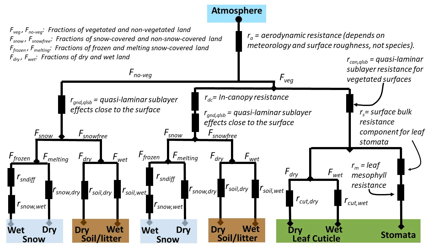
Figure B3Resistance diagram for the U.S. EPA CMAQ model with the STAGE deposition option. Note that this is an extension of the Massad et al. (2010) and Nemitz et al. (2001) resistance model in the CMAQ modelling framework.
Table B3AQMEII4-reported gaseous deposition variables corresponding to the CMAQ STAGE resistance model of Fig. B3.
; vegetation coverage fractions.
; snow coverage fraction.
; surface wetness fractions.
; snowmelt fractions.
Note that the vegetated fraction and leaf area index used in the above
equations for CMAQ with the STAGE deposition option are for specific LULC
types: the quantities in Table B3 will be reported for each of the 16
generic LULC categories for AQMEII4. Note that the lower canopy pathway has
been identified as such due to the presence of the rdc term; i.e. this
points to its similarity with Wesely's original lower canopy pathway.
B4 Example 4. LOTOS EUROS
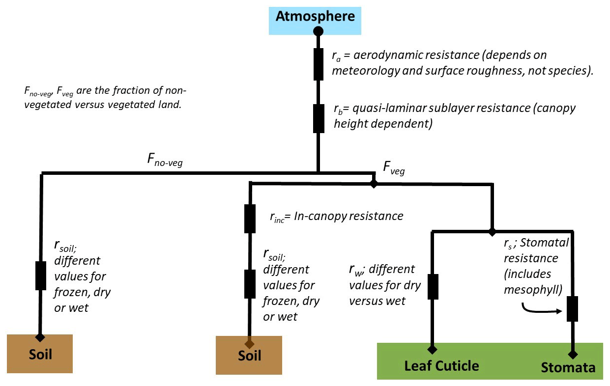
Table B4AQMEII4-reported gaseous deposition variables corresponding to the LOTOS-EUROS resistance model of Fig. B4.
B5 Example 5: GEM-MACH model, Zhang scheme
These are the calculations for the Environment and Climate Change Canada model GEM-MACH (Global Environmental Multiscale- Modelling Air-quality and CHemistry), using the scheme of Zhang et al. (2002, 2003, 2010). The resistance diagram for this model is shown in Fig. B5.
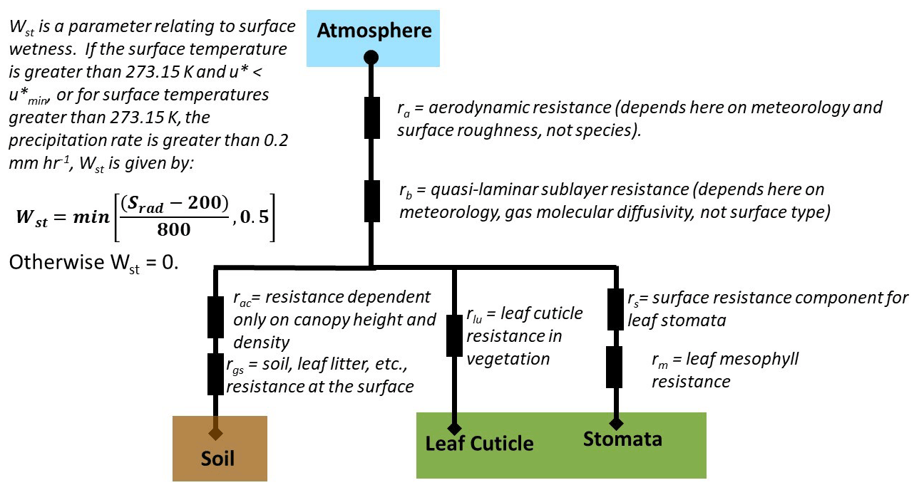
Table B5AQMEII4-reported gaseous deposition variables corresponding to the GEM-MACH Zhang resistance model of Fig. B5.
The main difference in the overall construction of the deposition scheme relative to the default Robichaud scheme (aside from the details of how the different terms are calculated) is in the absence of the lower canopy buoyant convection and exposed surface deposition branch of Wesely's original model. The details of the parameterizations for the terms in the equations also differ from the Robichaud scheme.
B6 Example 6. WRF-Chem

Table B6AQMEII4-reported gaseous deposition variables corresponding to the WRF-Chem resistance model of Fig. B6.
Prescribed values (table data) [pollutant, season]. rcl: for exposed surfaces in the lower canopy SO2, O3. rac: for transfer that depends on canopy height and density. rgs: for ground surfaces SO2, O3. rsi: for stomatal resistance.
rlu: for outer surfaces in
the upper canopy. H: Henry's law constant.
fi: reactivity factor.
B7 Example 7. COSMO-MUSCAT

Table B7AQMEII4-reported gaseous deposition variables corresponding to the COSMO-MUSCAT resistance model of Fig. B8.
Resistances provided by COSMO (calculated by the “TKE-based surface transfer scheme” for water vapour). ra: aerodynamic resistance (depends on meteorology, not species). rb: quasi-laminar sublayer resistance (depends on gas diffusivity; H2O dependency is adjusted by gas diffusivity constants of the corresponding species). rcut: net cuticle resistance (“roughness layer” resistance over vegetation). rac: resistance dependent only on canopy height and density (“roughness layer” resistance over non-vegetation).
B7.1 The TKE-based surface transfer scheme (for water vapour)
The surface-layer scheme used in COSMO is intimately related to the TKE scheme. Here, the surface layer is defined to be the layer of air between the earth surface and the lowest model level. We subdivide the surface layer into a laminar-turbulent sub-layer, the roughness layer, and a constant-flux or Prandtl layer above. The roughness layer extends from the non-planar irregular surface, where the turbulent distance is the turbulent length scale and κ is the von Kármán constant) is zero, up to a level l=H, such that l is proportional to the vertical height z within the Prandtl layer above. We choose to be equal to the dynamical roughness length z0. The lower boundary of the constant-flux layer (and of the atmospheric model) is defined to be a planar surface at a turbulent distance l=H from the surface. This subdivision allows us to discriminate between the values of the model variables at the rigid surfaces (predicted by the soil model) and values at the level l=H, which are “seen” by the atmosphere. For both layers, the fluxes are written in resistance form, where a roughness layer resistance is acting for scalar properties but not for momentum. Specific interpolation schemes are used to calculate the transport resistances of the layers. The applied surface scheme does not make use of empirical Monin–Obukhov stability functions, rather it generates these functions by the use of the dimensionless coefficients of the Mellor–Yamada closure and the interpolation rules.
The roughness layer is the region of the atmosphere into which vegetation and/or buildings protrude.
If a bidirectional flux algorithm for ammonia is employed in the model, then the flux may be either downwards (defined as positive here) or upwards (defined as negative, here). The generic equation for the bidirectional flux with this directionality is
where FT is the net flux, ca and cc are the atmospheric and canopy compensation point concentrations of ammonia gas, and rsum is a sum of resistances. Different sources in the literature make use of different formulas for both cc and rsum. For example, Zhang et al. (2010) employ
where cs and cg are compensation point concentrations relative to stomata and ground, respectively, and all other terms are defined as above. In contrast, CMAQ with the M3dry deposition option uses (Bash et al., 2013; Pleim et al., 2013, 2019)
where the variables A, B, and C in the quadratic of Eq. (C3) are given by
The variables used to generate the coefficients in Eq. (C4) for the CMAQ M3dry option are given by
where the terms rsoil, Heff, ah, , and Rwo are defined in Pleim et al. (2013). Note that in the latter reference (their Eq. 20), the summation term in Eq. (C4) above Gaca is repeated twice within the bracketed terms (i.e. as above is written , but this second occurrence of Gaca is likely a typo).
CMAQ with the STAGE deposition option closely follows the widely used Massad et al. (2010) and Nemitz et al. (2001) parameterizations modified to include the option for a cuticular compensation point and employs the same resistance model for all deposited species as it reduced to RES-SURF from Table B3 when the stomatal, Cs, cuticular, Ccut, and ground, Cg, compensation points are zero. NH3 bidirectional flux from the cuticle has been shown to be important (cuticular NH3 reference); however parameterizations applicable in a regional-scale model do not yet exist.
Cleaf is the leaf compensation point and is estimated by solving for the exchange between the canopy compensation point and the atmosphere, stomata, cuticle, and ground following Kirchhoff's current law (e.g. Nemitz et al., 2000). Cleaf is solved from this system of equations as follows.
The resistances rcut, rcan, qlsb, and rgnd, qlsb are taken from Massad et al. (2010). rdc follows Shuttleworth and Wallace (1985) but integrating the canopy transport model of Yi (2008) using the in-canopy eddy diffusivity of Bash et al. (2010) from the soil surface to top of the canopy and assuming . The remainder of the resistances are the same as CMAQ with the M3dry deposition option.
Comparing approaches (Eqs. C2 through C10), rsum, ra, and cc are held in common, and these approaches also make use of a stomatal (cs) and ground (cg) compensation point concentration, although how these terms are combined varies considerably between these approaches. For this reason, these common terms are reported as a separate TSD for ammonia bidirectional fluxes in AQMEII4 in order to allow cross-comparison of different approaches.
Note that the net flux of ammonia FT appears as DFLUX-NH3 in the AQMEII4 documentation provided to participants as TSDs and may be positive or negative depending on direction. Ammonia values for rb, net canopy resistance, stomatal resistance, mesophyll resistance, cuticle resistance, and the three effective conductances also appear elsewhere in the TSDs, both for the grid scale and by AQMEII4 LULC category.
No datasets were used in this article.
SG, PM, OEC, and CH led the writing of this technical note. SG, PM, OEC, CH, RB, RB, JB, JD, JF, CDH, IK, DS, and SS conceptualized and implemented the AQMEII4 modelling and analysis framework. JOB, TB, AH, RK, AL, JLPC, JP<YHR, RSJ, MGV, and RW provided documentation of dry deposition schemes used in their models.
The authors declare that they have no conflict of interest.
The views expressed in this paper are those of the authors and do not
necessarily represent the view or policies of the U.S. Environmental
Protection Agency. This material is based upon work supported, in part, by
the National Center for Atmospheric Research, which is a major facility
sponsored by the National Science Foundation under cooperative agreement no.
1852977.
Publisher’s note: Copernicus Publications remains neutral with regard to jurisdictional claims in published maps and institutional affiliations.
This article is part of the special issue “AQMEII-4: A detailed assessment of atmospheric deposition processes from point to the regional-scale models”. It is not associated with a conference.
We gratefully acknowledge the contribution of various groups to the fourth AQMEII activity. The following groups contributed the datasets used in the grid modelling aspects of this study: U.S. EPA and Environment and Climate Change Canada (North American emissions processing); TNO (European emissions processing); ECMWF and Copernicus Atmosphere Monitoring Service (Chemical boundary conditions); ECCAD (archiving and distribution of the GEIA lightning emissions data based on Price et al. (1997)); and Finnish Meteorological Institute (European wildfire emissions). Ambient North American concentration measurements were extracted from Environment Canada's National Atmospheric Chemistry Database (NAtChem) PM database and provided by several US and Canadian agencies (AQS, CAPMoN, CASTNet, IMPROVE, NAPS, SEARCH, and CSN networks). North American precipitation-chemistry measurements were extracted from NAtChem's precipitation-chemistry database and were provided by several US and Canadian agencies (CAPMoN, NADP, NBPMN, NSPSN, and REPQ networks). The WMO World Ozone and Ultraviolet Data Centre (WOUDC) and its data-contributing agencies provided North American and European ozonesonde profiles. For European air quality data the following data centres were used: EMEP European Environment Agency/European Topic Center on Air and Climate Change/AirBase provided European air- and precipitation-chemistry data. Data from meteorological station monitoring networks were obtained from NOAA and Environment and Climate Change Canada (for the US and Canadian meteorological network data) and the National Center for Atmospheric Research (NCAR) Data Support Section. The Joint Research Center Ispra/Institute for Environment and Sustainability provided its ENSEMBLE system for model output harmonization and analyses and evaluation.
This paper was edited by Joshua Fu and reviewed by two anonymous referees.
Anav, A., Proietti, C., Menut, L., Carnicelli, S., De Marco, A., and Paoletti, E.: Sensitivity of stomatal conductance to soil moisture: implications for tropospheric ozone, Atmos. Chem. Phys., 18, 5747–5763, https://doi.org/10.5194/acp-18-5747-2018, 2018.
Andersson, C. and Engardt, M.: European ozone in a future climate: Importance of changes in dry deposition and isoprene emissions, J. Geophys. Res., 115, D02303, https://doi.org/10.1029/2008JD011690, 2010.
Appel, K. W., Bash, J. O., Fahey, K. M., Foley, K. M., Gilliam, R. C., Hogrefe, C., Hutzell, W. T., Kang, D., Mathur, R., Murphy, B. N., Napelenok, S. L., Nolte, C. G., Pleim, J. E., Pouliot, G. A., Pye, H. O. T., Ran, L., Roselle, S. J., Sarwar, G., Schwede, D. B., Sidi, F. I., Spero, T. L., and Wong, D. C.: The Community Multiscale Air Quality (CMAQ) model versions 5.3 and 5.3.1: system updates and evaluation, Geosci. Model Dev., 14, 2867–2897, https://doi.org/10.5194/gmd-14-2867-2021, 2021.
Bash, J. O., Walker, J. T., Katul, G. G., Jones, M. R., Nemitz, E., and Robarge, W. P.: Estimation of in-canopy ammonia sources and sinks in a fertilized Zea mays field, Environ. Sci. Technol., 44, 1683–168, 2010.
Bash, J. O., Cooter, E. J., Dennis, R. L., Walker, J. T., and Pleim, J. E.: Evaluation of a regional air-quality model with bidirectional NH3 exchange coupled to an agroecosystem model, Biogeosciences, 10, 1635–1645, https://doi.org/10.5194/bg-10-1635-2013, 2013.
Baublitz, C. B., Fiore, A. M., Clifton, O. E., Mao, J., Li, J., Correa, G., Westervelt, D., Horowitz, L. W., Paulot, F., Commane, R., and Williams, A. P.: Sensitivity of tropospheric ozone over the Southeast USA to dry deposition, Geophys. Res. Lett., 47, e2020GL087158, https://doi.org/10.1029/2020GL087158, 2020.
Beddows, A. V., Kitwiroon, N., Williams, M. L., and Beevers, S. D.: Emulation and sensitivity analysis of the community multiscale air quality model for a UK Ozone pollution episode, Environ. Sci. Technol., 51, 6229–6236, 2017.
Blakeslee, R. J., Mach, D. M., Bateman, M. G., and Bailey, J. C.: Seasonal variations in the lightning diurnal cycle and implications for the global electric circuit, Atmos. Res., 135–136, 228–243, https://doi.org/10.1016/j.atmosres.2012.09.023, 2014.
Borrell, P. and Borrell, P. M. (Eds.): Transport and Chemical Transformation of Pollutants in the Troposphere, An Overview of the Work of EUROTRAC, Springer, Berlin, 474, https://doi.org/10.1007/978-3-642-59718-3, 2000.
Briggs, G. A.: Some Recent Analyses of Plume Rise Observation, in Proceedings of the Second International Clean Air Congress, edited by: Englun, H. M. and Beery, W. T., Academic Press, New York, 1029–1032, 1971.
Briggs, G. A.: Discussion on Chimney Plumes in Neutral and Stable Surroundings, Atmos. Environ., 6, 507–510, 1972.
Campbell, P. C., Bash, J. O., and Spero, T. L.: Updates to the Noah Land Surface Model in WRF-CMAQ to improve simulated meteorology, air quality, and deposition, J. Adv. Model. Earth Sy., 11, 231–256, https://doi.org/10.1029/2018MS001422, 2019.
Chang, J. S., Brost, R. A., Isaksen, I. S. A., Madronich, S., Middleton, P., Stockwell, W. R., and Walcek, C. J.: A three-dimensional Eulerian acid deposition model: Physical concepts and formulation, J. Geophys. Res., 92, 14681–14700, 1987.
Chen, J., Pavlovic, R., Anselmo, D., Beaulieu, P.-A., Gravel, S., Moran, M. D., and Davignon, D.: Development of on-line wildfire emissions for the operational Canadian air quality forecast system, 5th International Workshop on Air Quality Forecasting Research, 8–9 October, Santiago, Chile, 2013.
Chen, Y., Wolke, R., Ran, L., Birmili, W., Spindler, G., Schröder, W., Su, H., Cheng, Y., Tegen, I., and Wiedensohler, A.: A parameterization of the heterogeneous hydrolysis of N2O5 for mass-based aerosol models: improvement of particulate nitrate prediction, Atmos. Chem. Phys., 18, 673–689, https://doi.org/10.5194/acp-18-673-2018, 2018.
Clifton, O. E., Fiore, A. M., Munger, J. W., Malyshev, S., Horowitz, L. W., Shevliakova, E., Paulot, F., Murray, L. T., and Griffin, K. L.: Interannual variability in ozone removal by a temperate deciduous forest, Geophys. Res. Lett., 44, 542–552, https://doi.org/10.1002/2016GL070923, 2017.
Clifton, O. E., Fiore, A. M., Massman, W. J., Baublitz, C. B., Coyle, M., Emberson, L., Fares, S., Farmer, D. K., Gentine, P., Gerosa, G, Guenther, A. B., Helmig, D., Lombardozzi, D. L., Munger, J. W., Patton, E. G., Pusede, S. E., Schwede, D. B., Silva, S. J., Sörgel, M., Steiner, A. L., and Tai, A. P. K.: Dry deposition of ozone over land: processes, measurement, and modeling, Rev. Geophys., 58, e2019RG000670, https://doi.org/10.1029/2019RG000670, 2020a.
Clifton, O. E., Paulot, F., Fiore, A. M., Horowitz, L. W., Correa, G., Fares, S., Goded, I., Goldstein, A. H., Gruening, C., Hogg, A. J., Loubet, B., Mammarella, I., Munger, J. W., Neil, L., Stella, P., Uddling, J., Vesala, T., and Weng, E.: Influence of dynamic ozone dry deposition on ozone pollution, J. Geophys. Res.-Atmos., 125, e2020JD032398, https://doi.org/10.1029/2020JD032398, 2020b.
Dennis, R., Fox, T., Fuentes, M., Gilliland, A., Hanna, S., Hogrefe, C., Irwin, J., Rao, S. T., Scheffe, R., Schere, K., Steyn, D., and Venkatram, A.: A framework for evaluating regional-scale numerical photochemical modeling systems, Environ. Fluid Mech., 10, 471–489, https://doi.org/10.1007/s10652-009-9163-2, 2010.
Emberson, L. D., Kitwiroon, N., Beevers, S., Büker, P., and Cinderby, S.: Scorched Earth: how will changes in the strength of the vegetation sink to ozone deposition affect human health and ecosystems?, Atmos. Chem. Phys., 13, 6741–6755, https://doi.org/10.5194/acp-13-6741-2013, 2013.
Emberson, L. D., Pleijel, H., Ainsworth, E. A., van den Berg, M., Ren, W., Osborne, S., Mills, G., Pandey, D., Dentener, F., Büker, P., Ewert, F., Koeble, R., and Van Dingenen, R.: Ozone effects on crops and consideration in crop models, Eur. J. Agron., 100, 19–34, 2018.
Emerson, E. W., Hodshire, A. L., DeBolt, H. M., Bilsback, K. R., Pierce, J. R., McMeeking, G. R., and Farmer, D. K.: Revisiting particle dry deposition and its role in radiative effect estimates, P. Natl. Acad. Sci. USA, 117, 26076–26082, https://doi.org/10.1073/pnas.2014761117, 2020.
Erisman, J. W.: Evaluation of a surface resistance parameterization for sulphur dioxide, Atmos. Environ., 28, 2583–2594, 1994.
Fast, J. D., Gustafson Jr., W. I., Easter Jr., R. C., Zaveri, R. A., Barnard, J. C., Chapman, E. G., Grell, G., and Peckham, S. E.: Evolution of ozone, particulates, and aerosol direct radiative forcing in the vicinity of Houston using a fully coupled meteorology–chemistry–aerosol model, J. Geophys. Res.-Atmos., 111, D21305, https://doi.org/10.1029/2005JD006721, 2006.
Galmarini S., Rao, S. T., and Steyn, D. G.: Preface, Atmos. Environ., 53, 1–3, 2012.
Galmarini S., Hogrefe, C., Brunner, D., Makar, P., Baklanov, A.: Preface, Atmos. Environ., 115, 340–344, 2015.
Galmarini, S., Koffi, B., Solazzo, E., Keating, T., Hogrefe, C., Schulz, M., Benedictow, A., Griesfeller, J. J., Janssens-Maenhout, G., Carmichael, G., Fu, J., and Dentener, F.: Technical note: Coordination and harmonization of the multi-scale, multi-model activities HTAP2, AQMEII3, and MICS-Asia3: simulations, emission inventories, boundary conditions, and model output formats, Atmos. Chem. Phys., 17, 1543–1555, https://doi.org/10.5194/acp-17-1543-2017, 2017.
Grell, G., Peckham, S., Schmitz, R., McKeen, S., Frost, G., Skamarock, W., and Eder, B.: Fully coupled “online” chemistry within the WRF model, Atmos. Environ., 39, 6957–6975, https://doi.org/10.1016/j.atmosenv.2005.04.027, 2005.
Hardacre, C., Wild, O., and Emberson, L.: An evaluation of ozone dry deposition in global scale chemistry climate models, Atmos. Chem. Phys., 15, 6419–6436, https://doi.org/10.5194/acp-15-6419-2015, 2015.
Hodzic, A., Aumont, B., Knote, C., Lee-Taylor, J., Madronich, S., and Tyndall, G.: Volatility dependence of Henry's law constants of condensable organics: Application to estimate depositional loss of secondary organic aerosols, Geoph. Res. Lett., 41, 4795–4804, 2014.
Hogrefe, C., Liu, P., Pouliot, G., Mathur, R., Roselle, S., Flemming, J., Lin, M., and Park, R. J.: Impacts of different characterizations of large-scale background on simulated regional-scale ozone over the continental United States, Atmos. Chem. Phys., 18, 3839–3864, https://doi.org/10.5194/acp-18-3839-2018, 2018.
Hogrefe, C., Galmarini, S., Solazzo, E., Bianconi, R., Bellasio, R., Liu, P., and Mathur, R.: Continental-Scale Analysis of Atmospheric Deposition Over North America and Europe Using the AQMEII Database, in: Air Pollution Modeling and its Application XXVI, ITM 2018, edited by: Mensink, C., Gong, W., and Hakami, A., Springer Proceedings in Complexity, Springer, Cham, https://doi.org/10.1007/978-3-030-22055-6_48, 2020.
Hong, C., Mueller, N. D., Burney, J. A., Zhang, Y., AghaKouchak, A., Moore, F. C., Qin, Y., Tong, D., and Davis, S. J.: Impacts of ozone and climate change on yields of perennial crops in California, Nature Food, 1, 166–172, 2020.
Huang, L., McDonald-Buller, E. C., McGaughey, G., Kimura, Y., and Allen, D. T.: The impact of drought on ozone dry deposition over eastern Texas, Atmos. Environ., 127, 176–186, https://doi.org/10.1016/j.atmosenv.2015.12.022, 2016.
Inness, A., Ades, M., Agustí-Panareda, A., Barré, J., Benedictow, A., Blechschmidt, A.-M., Dominguez, J. J., Engelen, R., Eskes, H., Flemming, J., Huijnen, V., Jones, L., Kipling, Z., Massart, S., Parrington, M., Peuch, V.-H., Razinger, M., Remy, S., Schulz, M., and Suttie, M.: The CAMS reanalysis of atmospheric composition, Atmos. Chem. Phys., 19, 3515–3556, https://doi.org/10.5194/acp-19-3515-2019, 2019.
Irving, P. M. and Smith, E.: Acid deposition: State of science and technology Summary report of the US National Acid Precipitation Assessment Program, US Govt. Printing Office, United States, ISBN 0-16-035925-2, 274 pp., 1991.
Jarvis, P. G.: The interpretation of the variations in leaf water potential and stomatal conductance found in canopies in the field, Philos. T. R. Soc. Lond. B., 273, 593–610, 1976.
Knote, C., Hodzic, A., Jimenez, J. L., Volkamer, R., Orlando, J. J., Baidar, S., Brioude, J., Fast, J., Gentner, D. R., Goldstein, A. H., Hayes, P. L., Knighton, W. B., Oetjen, H., Setyan, A., Stark, H., Thalman, R., Tyndall, G., Washenfelder, R., Waxman, E., and Zhang, Q.: Simulation of semi-explicit mechanisms of SOA formation from glyoxal in aerosol in a 3-D model, Atmos. Chem. Phys., 14, 6213–6239, https://doi.org/10.5194/acp-14-6213-2014, 2014.
Knote, C., Hodzic, A., and Jimenez, J. L.: The effect of dry and wet deposition of condensable vapors on secondary organic aerosols concentrations over the continental US, Atmos. Chem. Phys., 15, 1–18, https://doi.org/10.5194/acp-15-1-2015, 2015.
Kuenen, J., Visschedijk, A., and Denier van der Gon, H. A. C.: TNO_MACC-III inventory and its application for FAIRMODE SoAp, Fairmode technical meeting, Aveiro, Portugal, available at: https://aqm.jrc.ec.europa.eu/fairmode/document/event/presentation/20150624-Aveiro/WG3/WG3 Kuenen.pdf (last access: 8 October 2021), 2015.
Lin, M., Horowitz, L. W., Xie, Y., Paulot, F., Malyshev, S., Shevliakova, E., Finco, A., Gerosa, G., Kubistin, D., Pilegaard, K., Vegetation feedbacks during drought exacerbate ozone air pollution extremes in Europe, Nat. Clim., 10, 444–451, 2020.
Lombardozzi, D., Levis, S., Bonan, G., Hess, P. G., and Sparks, J. P., The Influence of Chronic Ozone Exposure on Global Carbon and Water Cycles, J. Climate, 28, 292–305, https://doi.org/10.1175/JCLI-D-14-00223.1, 2015.
Makar, P. A., Staebler, R. M., Akingunola, A., Zhang, J., McLinden, C., Kharol, S. K., Pabla, B., Cheung, P., and Zheng, Q.: The effects of forest canopy shading and turbulence on boundary layer ozone, Nat. Commun., 8, 15243, https://doi.org/10.1038/ncomms15243, 2017.
Makar, P. A., Akingunola, A., Aherne, J., Cole, A. S., Aklilu, Y.-A., Zhang, J., Wong, I., Hayden, K., Li, S.-M., Kirk, J., Scott, K., Moran, M. D., Robichaud, A., Cathcart, H., Baratzedah, P., Pabla, B., Cheung, P., Zheng, Q., and Jeffries, D. S.: Estimates of exceedances of critical loads for acidifying deposition in Alberta and Saskatchewan, Atmos. Chem. Phys., 18, 9897–9927, https://doi.org/10.5194/acp-18-9897-2018, 2018.
Makar, P. A., Stroud, C., Akingunola, A., Zhang, J., Ren, S., Cheung, P., and Zheng, Q.: Vehicle-induced turbulence and atmospheric pollution, Atmos. Chem. Phys., 21, 12291–12316, https://doi.org/10.5194/acp-21-12291-2021, 2021.
Manders, A. M. M., Builtjes, P. J. H., Curier, L., Denier van der Gon, H. A. C., Hendriks, C., Jonkers, S., Kranenburg, R., Kuenen, J. J. P., Segers, A. J., Timmermans, R. M. A., Visschedijk, A. J. H., Wichink Kruit, R. J., van Pul, W. A. J., Sauter, F. J., van der Swaluw, E., Swart, D. P. J., Douros, J., Eskes, H., van Meijgaard, E., van Ulft, B., van Velthoven, P., Banzhaf, S., Mues, A. C., Stern, R., Fu, G., Lu, S., Heemink, A., van Velzen, N., and Schaap, M.: Curriculum vitae of the LOTOS–EUROS (v2.0) chemistry transport model, Geosci. Model Dev., 10, 4145–4173, https://doi.org/10.5194/gmd-10-4145-2017, 2017.
Matichuk, R., Tonnesen, G., Luecken, D., Gilliam, R., Napelenok, S. L., Baker, K. R., Schwede, D., Murphy, B., Helmig, D., Seth, N., Lyman, S., and Roselle S.: Evaluation of the Community Multiscale Air Quality Model for simulating winter ozone formation in the Uinta Basin, J. Geophys. Res.-Atmos., 122, 13545–13572, https://doi.org/10.1002/2017JD027057, 2017.
Massad, R.-S., Nemitz, E., and Sutton, M. A.: Review and parameterisation of bi-directional ammonia exchange between vegetation and the atmosphere, Atmos. Chem. Phys., 10, 10359–10386, https://doi.org/10.5194/acp-10-10359-2010, 2010.
McGrath, J. M., Betzelberger A. M., Wang, S., Shook, E., Zhu, X. G., Long, S. P., and Ainsworth, E. A.: An analysis of ozone damage to historical maize and soybean yields in the United States, P. Natl. Acad. Sci. USA, 112, 14390–14395, 2015.
Moran, M. D., Menard, S., Talbot, D., Huang, P., Makar, P. A., Gong, W., Landry, H., Gravel, S., Gong, S., Crevier, L.-P., Kallaur, A., and Sassi, M.: Particulate-matter forecasting with GEM-MACH15, a new Canadian air-quality forecast model, in: Air Pollution Modelling and Its Application XX, edited by: Steyn, D. G. and Rao, S. T., Springer, Dordrecht, 289–292, 2010.
Nemitz, E., Sutton, M. A., Schjoerring, J. K., Husted, S., and Wyers, G. P.: Resistance modelling of ammonia exchange over oilseed rape, Agr. Forest Meteorol., 105, 405–425, 2000.
Nemitz, E., Milford, C., and Sutton, M. A.: A two-layer canopy compensation point model for describing bi-directional biosphere-atmosphere exchange of ammonia, Q. J. Roy. Meteor. Soc., 127, 815–833, 2001.
Oliver, R. J., Mercado, L. M., Sitch, S., Simpson, D. M., Medlyn, B. E., Lin, Y., and Folberth, G. A.: Large but decreasing effect of ozone on the European carbon sink, Biogeosciences, 4245–4269, 2018.
Ott, L. E., Pickering, K. E., Stenchikov, G. L., Allen, D. J., DeCaria, A. J., Ridley, B., Lin, R.-F., Lang, S., and Tao, W.-K.: Production of lightning NOx and its vertical distribution calculated from three-dimensional cloud-scale chemical transport model simulations, J. Geophys. Res., 115, D04301, https://doi.org/10.1029/2009JD011880, 2010.
Paulot, F., Malyshev, S., Nguyen, T., Crounse, J. D., Shevliakova, E., and Horowitz, L. W.: Representing sub-grid scale variations in nitrogen deposition associated with land use in a global Earth system model: implications for present and future nitrogen deposition fluxes over North America, Atmos. Chem. Phys., 18, 17963–17978, https://doi.org/10.5194/acp-18-17963-2018, 2018.
Pleim, J. E., Bash, J. O., Walker, J. T., and Cooter, E. J.: Development and evaluation of an ammonia bidirectional flux parameterization for air quality models, J. Geophys. Res.-Atmos., 118, 3794–3806, 2013.
Pleim, J. E., Ran, L., Appel, W., Shephard, M. W., and Cady-Pereira, K., New bidirectional ammonia flux model in an air quality model coupled with an agricultural model, J. Adv. Model. Earth Sy., 11, 2934–2957, https://doi.org/10.1029/2019MS001728, 2019.
Price, C. G., Penner, J. E., and Prather, M. J.: NOx from lightning, Part I: Global distribution based on lightning physics, J. Geophys. Res., 102, 5229–5241, 1997.
Rao, S. T., Galmarini, S., and Puckett, K.: Air quality model evaluation international initiative (AQMEII), B. Am. Meteorol. Soc., 92, 23–30, https://doi.org/10.1175/2010BAMS3069.1, 2011.
Robichaud, A., Cole, A., Moran, M., Lupu, A., Shaw, M., Roy, G., Beauchemin, M., Fortin, V., and Vet, R.: Total deposition maps evaluated from measurement-model fusion in North America (ADAGIO Project), edited by: Mensink C., Gong W., and Hakami A., in: Air Pollution Modeling and its Application XXVI, ITM, Springer Proceedings in Complexity. Springer, Cham, https://doi.org/10.1007/978-3-030-22055-6_40, 2020a.
Robichaud, A., Cole, A. S., Moran, M. D., Lupu, A., Beauchemin, M., and Fortin, V.: On model-data fusion approaches for wet deposition in North America, National Atmospheric Deposition Program Scientific Symposium and Fall Meeting, 28–30, October 2020, available at: http://nadp.slh.wisc.edu/conf/2020/?sID=6 (last access: 23 March 2021), 2020b.
Saylor, R. D., Baker, B. D., Lee, P., Tong, D., Pan, L., and Hicks, B. B.: The particle dry deposition component of total deposition from air quality models: right, wrong or uncertain?, Tellus B, 71, 1550324, https://doi.org/10.1080/16000889.2018.1550324, 2019.
Schiferl, L. D. and Heald, C. L.: Particulate matter air pollution may offset ozone damage to global crop production, Atmos. Chem. Phys., 18, 5953–5966, https://doi.org/10.5194/acp-18-5953-2018, 2018.
Schwede, D. B. and Lear, G. G.: A novel hybrid approach for estimating total deposition in the United States, Atmos. Environ., 92, 207–220, 2014.
Sharma, A., Ojha, N., Ansari, T. U., Sharma, S. K., Pozzer, A., and Gunthe, S. S.: Effects of dry deposition on surface ozone over South Asia inferred from a regional chemical transport model, ACS Earth and Space Chemistry, 4, 321–327, 2020.
Shuttleworth, W. J. and Wallace, J. S.: Evaporation from sparse crops – an energy combination theory, Q. J. Roy. Meteor. Soc., 111, 839–855, 1985.
Silva, S. J. and Heald, C. L.: Investigating dry deposition of ozone to vegetation, J. Geophys. Res.-Atmos., 123, 559–573, https://doi.org/10.1002/2017JD027278, 2018.
Soares, J., Sofiev, M., and Hakkarainen, J.: 2015. Uncertainties of wild-land fires emission in AQMEII phase 2 case study, Atmos. Environ., 115, 361–370, https://doi.org/10.1016/j.atmosenv.2015.01.068, 2015.
Solazzo, E., Riccio, A., Van Dingenen, R., Valentini, L., and Galmarini, S.: Evaluation and uncertainty estimation of the impact of air quality modelling on crop yields and premature deaths using a multi-model ensemble, Sci. Total Environ., 633, 1437–1452, 2018.
Solazzo, E., Hogrefe, C., Colette, A., Garcia-Vivanco, M., and Galmarini, S.: Advanced error diagnostics of the CMAQ and Chimere modelling systems within the AQMEII3 model evaluation framework, Atmos. Chem. Phys., 17, 10435–10465, https://doi.org/10.5194/acp-17-10435-2017, 2017.
Solberg, S., Hov, Ø., Søvdee, A., Isaksen, I. S. A., Coddevillee, P., De Backer, H., Forster, C., Orsolini, Y., and Uhse, K., European surface ozone in the extreme summer 2003, J. Geophys. Res., 113, D07307, https://doi.org/10.1029/2007JD009098, 2008.
United States Environmental Protection Agency: CMAQ (Version 5.3.1) [software], https://doi.org/10.5281/zenodo.3585898, 2019.
Val Martin, M., Heald, C. L., and Arnold, S. R.: Coupling dry deposition to vegetation phenology in the Community Earth System Model: Implications for the simulation of surface O3, Geophys. Res. Lett., 41, 2988–2996, 2014.
Vautard, R., Honore, C., Beekmann, M., and Rouil, L.: Simulation of ozone during the August 2003 heat wave and emission control scenarios, Atmos. Environ., 39, 2957–2967, 2005.
Vivanco, M. G., Theobald, M. R., García-Gómez, H., Garrido, J. L., Prank, M., Aas, W., Adani, M., Alyuz, U., Andersson, C., Bellasio, R., Bessagnet, B., Bianconi, R., Bieser, J., Brandt, J., Briganti, G., Cappelletti, A., Curci, G., Christensen, J. H., Colette, A., Couvidat, F., Cuvelier, C., D'Isidoro, M., Flemming, J., Fraser, A., Geels, C., Hansen, K. M., Hogrefe, C., Im, U., Jorba, O., Kitwiroon, N., Manders, A., Mircea, M., Otero, N., Pay, M.-T., Pozzoli, L., Solazzo, E., Tsyro, S., Unal, A., Wind, P., and Galmarini, S.: Modeled deposition of nitrogen and sulfur in Europe estimated by 14 air quality model systems: evaluation, effects of changes in emissions and implications for habitat protection, Atmos. Chem. Phys., 18, 10199–10218, https://doi.org/10.5194/acp-18-10199-2018, 2018.
Wesely, M. L.: Parameterization of surface resistances to gaseous dry deposition in regional-scale numerical models, Atmos. Environ., 23, 1293–1304, 1989.
Wichink Kruit, R. J., Schaap, M., Sauter, F. J., van Zanten, M. C., and van Pul, W. A. J.: Modeling the distribution of ammonia across Europe including bi-directional surface–atmosphere exchange, Biogeosciences, 9, 5261–5277, https://doi.org/10.5194/bg-9-5261-2012, 2012.
Wolke, R., Schröder, W., Schrödner, R., and Renner, E.: Influence of grid resolution and meteorological forcing on simulated European air quality: A sensitivity study with the modeling system COSMO-MUSCAT, Atmos. Environ., 53, 110–130, 2012.
Wong, A. Y. H., Geddes, J. A., Tai, A. P. K., and Silva, S. J.: Importance of dry deposition parameterization choice in global simulations of surface ozone, Atmos. Chem. Phys., 19, 14365–14385, https://doi.org/10.5194/acp-19-14365-2019, 2019.
Wu, Z., Schwede, D. B., Vet, R., Walker, J. T., Shaw, M., Staebler, R., and Zhang, L., Evaluation and intercomparison of five North American dry deposition algorithms at a mixed forest site, J. Adv. Model Earth Sy., 10, 1571–1586, https://doi.org/10.1029/2017MS001231, 2018.
Yi, C.: Momentum transfer within canopies, J. Appl. Meteorol. Clim., 47, 262–275, 2008.
Zhang, L., Moran, M. D., Makar, P. A., Brook, J. R., and Gong, S.: Modelling gaseous dry deposition in AURAMS: a unified regional air-quality modelling system, Atmos. Environ., 36, 537–560, 2002.
Zhang, L., Brook, J. R., and Vet, R.: A revised parameterization for gaseous dry deposition in air-quality models, Atmos. Chem. Phys., 3, 2067–2082, https://doi.org/10.5194/acp-3-2067-2003, 2003.
Zhang, L., Wright, L. P., and Asman, W. A. H.: Bi-directional air-surface exchange of atmospheric ammonia: A review of measurements and a development of a big-leaf model for applications in regional-scale air-quality models, J. Geophys. Res., 115, D20310, https://doi.org/10.1029/2009JD013589, 2010.
Note that the depositing gases in each pathway are influenced by ra and rb prior to encountering the different resistances that make up rc, and this is why vd, which includes the influence of ra and rb, is scaled by the fraction of the inverse of rc occurring through a given pathway. Some models include surface-specific quasi-laminar sublayer resistances; when this is the case, these terms appear in the pathway-specific fractions of the total uptake terms.
- Abstract
- Introduction
- AQMEII4 Activity 1 description
- Strategy for the diagnostic intercomparison of dry deposition from different grid-based models
- More example calculations of AQMEII4 dry deposition variables
- Conclusions
- Appendix A: Standard output requested from all participating models
- Appendix B: Resistance diagrams and calculation of AQMEII4 reported dry deposition diagnostic variables for dry deposition schemes implemented in participating models
- Appendix C: Bidirectional ammonia fluxes
- Data availability
- Author contributions
- Competing interests
- Disclaimer
- Special issue statement
- Acknowledgements
- Review statement
- References