the Creative Commons Attribution 4.0 License.
the Creative Commons Attribution 4.0 License.
 | 18 Oct 2021
Evaluating the impact of storage-and-release on aircraft-based mass-balance methodology using a regional air-quality model
Sepehr Fathi
Mark Gordon
Paul A. Makar
Ayodeji Akingunola
Andrea Darlington
John Liggio
Katherine Hayden
Shao-Meng Li
We investigate the potential for aircraft-based top-down emission rate retrieval over- and under-estimation using a regional chemical transport model, the Global Environmental Multiscale-Modeling Air-Quality and CHemistry (GEM-MACH). In our investigations we consider the application of the mass-balance approach in the Top-down Emission Rate Retrieval Algorithm (TERRA). Aircraft-based mass-balance retrieval methodologies such as TERRA require relatively constant meteorological conditions and source emission rates to reliably estimate emission rates from aircraft observations. Avoiding cases where meteorology and emission rates change significantly is one means of reducing emissions retrieval uncertainty, and quantitative metrics that may be used for retrieval accuracy estimation are therefore desirable. Using these metrics has the potential to greatly improve emission rate retrieval accuracy. Here, we investigate the impact of meteorological variability on mass-balance emission rate retrieval accuracy by using model-simulated fields as a proxy for real-world chemical and meteorological fields, in which virtual aircraft sampling of the GEM-MACH output was used for top-down mass balance estimates. We also explore the impact of upwind emissions from nearby sources on the accuracy of the retrieved emission rates. This approach allows the state of the atmosphere used for top-down estimates to be characterized in time and 3D space; the input meteorology and emissions are “known”, and thus potential means for improving emission rate retrievals and determining the factors affecting retrieval accuracy may be investigated. We found that emissions retrieval accuracy is correlated with three key quantitative criteria, evaluated a priori from forecasts and/or from observations during the sampling period: (1) changes to the atmospheric stability (described as the change in gradient Richardson number), (2) variations in the direction of transport, as a result of plume vertical motion and in the presence of vertical wind shear, and (3) the combined effect of the upwind-to-downwind concentration ratio and the upwind-to-downwind concentration standard deviations. We show here that cases where these criteria indicate high temporal variability and/or high upwind emissions can result in “storage-and-release” events within the sampled region (control volume), which decrease emission rate retrieval accuracy. Storage-and-release events may contribute the bulk of mass-balance emission rate retrieval under- and over-estimates, ranging in the tests carried out here from −25 % to 24 % of the known (input) emissions, with a median of −2 %. Our analysis also includes two cases with unsuitable meteorological conditions and/or significant upwind emissions to demonstrate conditions which may result in severe storage, which in turn cause emission rate under-estimates by the mass-balance approach. We also introduce a sampling strategy whereby the emission rate retrieval under- and over-estimates associated with storage-and-release are greatly reduced (to −14 % to +5 %, respectively, relative to the magnitude of the known emissions). We recommend repeat flights over a given facility and/or time-consecutive upwind and downwind (remote) vertical profiling of relevant fields (e.g., tracer concentrations) in order to measure and account for the factors associated with storage-and-release events, estimate the temporal trends in the evolution of the system during the flight/sampling time, and partially correct for the effects of meteorological variability and upwind emissions.
- Article
(7587 KB) - Full-text XML
- BibTeX
- EndNote


Aircraft-based measurements of air pollutants provide an effective top-down approach for estimating total integrated emissions of sources ranging from individual stacks to large industrial complexes and cities. These top-down estimates are commonly employed for the evaluation of bottom-up emissions reported to inventories and can provide insights into air quality and health impacts of anthropogenic emissions. Top-down estimates can also be used to provide highly resolved emissions data for input into air-quality models. Several studies have utilized aircraft-based top-down emission rate retrievals in the past (Kalthoff et al., 2002; Mays et al., 2009; Turnbull et al., 2011; Karion et al., 2013, 2015; Cambaliza et al., 2014; Gordon et al., 2015; Nathan et al., 2015; Tadić et al., 2017; Conley et al., 2017; Ryoo et al., 2019). Flight patterns from these studies include single-height transects, single-screen flights and box flights. Box flights, which expand upon “single-leg” (mainly downwind) flights, refer to flight patterns with enclosed shapes (polygonal, cylindrical) and are accomplished by flying in closed paths (loops) at multiple altitudes around the emission source while making measurements of meteorological fields and pollutant concentrations (Gordon et al., 2015; Tadić et al., 2017). The mass-balance technique and Gauss's divergence theorem – where the net mass flux of the species of interest exiting a control volume is equated to the within-volume source emission rates of that species – can be employed to infer point and area source emission rates from aircraft-measured data. Kalthoff et al. (2002) used aircraft-measured data to estimate CO and NOx emissions of the city of Augsburg in southern Germany, using data from two research aircrafts at several altitudes (polygonal box) around the boundaries of the city during the EVA project (Slemr et al., 2002). Emission rate estimations were made using a mass-balance approach applied to aircraft measurements, and estimates were used in improving emissions input data for an air-quality model (KAMM/DRAIS). Through air-quality model (KAMM/DRAIS) simulations, Panitz et al. (2002) analyzed the validity of the assumptions made by Kalthoff et al. (2002) and also studied the contributions of all relevant processes (advective fluxes, deposition, turbulent transports, and chemical transformations) to the mass budget of chemical species (e.g., CO and NOx). They concluded that, in an aircraft-based mass-balance approach, 85 % and 95 % of source emissions can be determined from the advective fluxes. Gordon et al. (2015) assessed uncertainties in the top-down aircraft-based emission rate retrievals using polygonal (e.g., rectangular) box flights measuring SO2 and CH4 around individual oil sands facilities in Alberta, Canada. This study also involved development of a methodology for extrapolation of aircraft-measured data below the lowest flight level based on various assumptions and the analysis of the associated uncertainties. Gordon et al. (2015) estimated uncertainty in aircraft-based estimates as 2 %–30 %, with the source of this uncertainty attributed mainly to extrapolation of aircraft measurements below the lowest flight track (20 %). Conley et al. (2017) and Ryoo et al. (2019) made aircraft-based emission estimations by flying cylindrical box flights around different point/area emission sources. The study by Conley et al. (2017) also involved evaluation and optimization of the sampling strategy (e.g., optimized circling radius) in order to minimize the uncertainties due to data extrapolation below the lowest flight level through controlled release of tracers and large eddy simulations (LES).
The potential for measurement error to affect retrieval accuracy has been discussed in the literature. Turnbull et al. (2011) noted that observation errors in wind-speed and planetary boundary layer height led to a factor of 2 estimated error in CO2 emissions retrievals. Ryoo et al. (2019) suggested that errors associated with wind speed errors and assumptions about background concentrations for greenhouse gases for city-scale emissions sources could contribute emissions retrieval errors for a factor of 1.5 to 7. However, Ryoo et al. (2019) also noted that these errors stem largely from the use of flight patterns consisting of downwind screens, and that flight patterns which enclose the sources, (closed shape flight patterns) such as the box flights used in our current work, greatly reduce these errors. Tadić et al. (2017) noted that cylindrical flight patterns around facilities (similar to “box” flights described in Gordon et al., 2015) provide superior retrieval performance relative to downwind screens. The strategy for determining the maximum height of aircraft flights also varies between references, some recommending sampling up to the PBL height. However, Tadić et al. (2017) and Gordon et al. (2015) integrate over the entire vertical extent of the plume (as in the work described here) rather than limit the analysis to below the planetary boundary layer height. Tadić et al. (2017) estimated the uncertainties in retrievals, calculated from flight patterns using these procedures, associated with different factors: interpolation uncertainties accounted for 21 % of the determined emissions value, while wind speed errors of 0.1 m s−1 were attributed to −1.2 % to +1.5 % of the retrieval error, respectively. The latter suggests that the impact of wind speed error, when box or cylinder flight patterns such as we use in our current work, is relatively small.
These and other similar studies, employed either mass transfer (e.g., the single-screen flight approach where the horizontal mass flux through a downwind vertical plane is equated to the upwind source emission rates) or a mass-balance approach (box flights) to infer point and area source emission rates from aircraft-measured data. Aircraft-based estimates are generally (and where possible) compared to bottom-up inventory reported emission data (e.g., Gordon et al., 2015; Li et al., 2017; Baray et al., 2018; Liggio et al., 2019; Cheng et al., 2020), and may also be evaluated using Continuous Emissions Monitoring System (CEMS) data (when these data are available). These comparisons and their conclusions are dependent in part on the magnitude of the uncertainty levels associated with the estimates. The algorithms for emission rate retrieval require steady-state meteorological and emissions data. Cases where these conditions are not met have been avoided through the application of a priori criteria in flight planning and post-flight retrieval decision making. For example, pre-flight decision criteria such as relatively invariant forecast wind speed, wind direction, and planetary boundary layer height, were used to determine “fly/no-fly” decisions in past studies (e.g., Li et al., 2017; Liggio et al., 2019). We refine these concepts here to create quantitative metrics for assessing retrieval success which may also be used in forecasting flight conditions or during flights. We also investigate the potential causes of emissions retrieval uncertainty, using a variety of cases, including unsuitable cases which would usually not be used for retrievals, as tests of our criteria. Therefore, it is important to further refine the methodology used to predict uncertainties in retrievals as well as suggest revised methodologies which may reduce emissions retrieval uncertainty. Uncertainties in aircraft-based top-down retrievals may arise from various sources (e.g., measurements, data interpolation and extrapolation), most of which have been studied in the past (e.g., Cambaliza et al., 2014; Gordon et al., 2015; Angevine et al., 2020). Prior studies have also noted the potential contribution of temporal trends in tracer mass budget to mass-balance retrievals (e.g., Conley et al., 2017), but mainly relied on the assumption of steady-state conditions. Here we focus on investigating the underlying assumption of time-invariant meteorological conditions (during observation time), which is shared among most (if not all) top-down retrieval methodologies, in particular the impact of localized variations in meteorology (e.g., change in atmospheric stability or direction of the transport) on the application of the mass-balance technique in box flight emission rate retrievals.
Under time-invariant and spatially uniform conditions, a mass-balance approach based on Gauss's divergence theorem equates the rate of emissions from sources within a control volume (box flight) to the net mass flux through the boundaries (box walls) by assuming the net rate of accumulation of mass within the volume to be negligible. When conditions (e.g., meteorology, emissions) deviate from steady-state and/or localized inhomogeneity is developed in tracer concentration and meteorological fields, the rate of mass accumulation/release within the control volume may become significant enough to affect the accuracy of the estimates based on the mass balance approach. Herein, we refer to these circumstances as “storage-and-release” events. To our knowledge, all mass-balance techniques to date assume steady-state conditions. Here we investigate the uncertainty associated with that assumption and we introduce the term storage-release (used interchangeably with storage-and-release throughout the paper) events for transient non-steady-state conditions. This term is chosen to emphasize the cyclical nature of the events, during which material within the control volume accumulated and is then subsequently released.
Numerical dispersion modelling has been proven useful in assessing the uncertainties in top-down retrievals in the past Panitz et al. (e.g., 2002) and more recently Karion et al. (e.g., 2019); Angevine et al. (e.g., 2020). Here, the numerical modelling system (a regional chemical transport model) we use is Environment and Climate Change Canada's (ECCC) air-quality model, Global Environmental Multiscale-Modeling Air-Quality and CHemistry (GEM-MACH). Through the use of GEM-MACH model 4D fields (known meteorology and input emissions), we have eliminated all other sources of uncertainty in the input information used to retrieve emissions (e.g., measurement error, interpolation) and have extensively explored the impact of storage-and-release events on aircraft-based top-down emission rate retrievals. We investigate the potential magnitude and the causes of emissions over- and under-estimates, using GEM-MACH model's input emissions and output concentrations as a proxy for aircraft observations. This approach allows us to more precisely examine the root causes of potential emissions retrieval over-/under-estimates, through making use of ancillary information provided by the model, which may not be available from past aircraft studies. Throughout this paper, as an example method, we refer to (and adopt schemes from) the aircraft-based retrieval methodology developed by ECCC and described in Gordon et al. (2015), the Top-down Emission Rate Retrieval Algorithm (TERRA). The concepts explored here are not specific to TERRA and are applicable to all top-down retrieval methodologies that use the mass-balance approach.
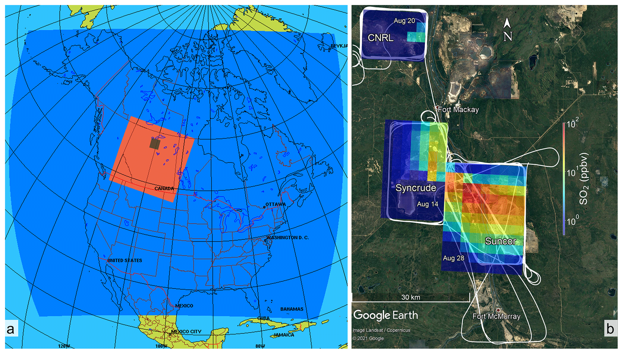
Figure 1(a) GEM-MACH model horizontal grid structure with nested domains: the dark blue region shows the parent domain over North America at 10 km horizontal grid resolution. Output from GEM-MACH 10 km simulations provided initial and boundary conditions for the nested high-resolution GEM-MACH 2.5 km domain (red). The high-resolution domain was configured over the Canadian provinces of Alberta and Saskatchewan including the Alberta Athabasca oil sands region, shown as a dark shaded area. (b) © Google Earth map of the region with three oil sands facilities labelled. JOSM 2013 flight tracks on 14, 20 and 28 August are drawn with white curves. Model 4D fields were extracted for nine JOSM 2013 box flight cases over these three facilities, examples are shown as overlay SO2 concentration maps.
During an aircraft campaign conducted in August and September of 2013 as part of the Joint Canada Alberta implementation plan for Oil Sands Monitoring (JOSM), the National Research Council of Canada Flight Research Laboratory (NRC-FRL) Convair 580 research aircraft was used to make air-quality measurements over the Athabasca oil sands region (Alberta, Canada). Air-quality forecasts created using ECCC's air-quality model GEM-MACH, provided advice on flight planning for the JOSM 2013 campaign (Makar et al., 2016). For this purpose, and for the post-study simulations conducted here, the GEM-MACH system was configured to create high-resolution nested air-quality forecasts with a fine-resolution domain (2.5 km) over the Canadian provinces of Alberta and Saskatchewan, including the Athabasca oil sands region (Fig. 1a). From 10 August to 10 September 2013 a total of 22 flights were conducted around and downwind of oil sands facilities, 13 of which were emission estimation (box) flights where the aircraft was flown around individual facilities at multiple altitudes, approximating a rectangular/polygonal shaped box (control volume), while making meteorological and air-quality measurements (JOSM, 2011). We chose our model input test cases from the same times and locations as JOSM 2013 box flights, to sample conditions (meteorology and emissions) similar to the range existing within the real atmosphere which might be considered for retrievals. Nine box flight cases over three oil sands facilities with significant SO2 emissions (Syncrude, CNRL and Suncor; see Fig. 1b) were chosen because (1) SO2 is emitted from stack sources but has low background levels (Gordon et al., 2015), reducing uncertainties in emission rate retrievals based on the mass-balance approach and (2) hourly SO2 emissions and stack parameter data are available from the CEMS reports (Zhang et al., 2018) thereby ensuring the GEM-MACH inputs are realistic: CEMS-derived input emissions in GEM-MACH resulted in improved model plume rise and transport representation (model-simulated plume heights were evaluated in Akingunola et al., 2018). Output data from GEM-MACH model simulations for the period of the nine cases were analyzed and mass-balance estimates of model SO2 input emissions were made. Model configuration and set-up and simulation scenarios for this work are described in Sect. 2.1. Section 2.2 describes the methodologies that were developed here for direct and virtual aircraft-based retrievals of model input emissions using the GEM-MACH model output fields as well as suggested improvements for flight planning.
2.1 Model description and simulations
ECCC's air-quality model, GEM-MACH, is a fully coupled online air-quality and chemical transport model. The GEM-MACH modelling system resides within the Global Environmental Multiscale (GEM) numerical weather prediction model (Côté et al., 1998b, a; Girard et al., 2014) and includes an atmospheric chemistry module (Moran et al., 2010) with gas and particle process representation. The details of the GEM-MACH configuration used here appear in Table A1. We note that this work is not intended as an evaluation of the GEM meteorological model and its components, which have been extensively evaluated elsewhere in the literature (e.g., Côté et al., 1998b; Bélair et al., 2003b, a; Li and Barker, 2005; Milbrandt and Yau, 2005a, b; Fillion et al., 2010; Girard et al., 2014; Milbrandt and Morrison, 2016). A recent detailed evaluation of GEM-MACH’s meteorological performance is also provided in Makar et al. (2021). Rather, we use the model as a proxy for observations since it can provide instantaneous 3D values for chemical concentrations and meteorological variables, which in turn allow us to construct parameters that can be used to predict storage-and-release events in observation-based applications.
For this work, a series of retrospective high-resolution nested air-quality simulations were made for the period of the JOSM summer 2013 aircraft intensive campaign (JOSM, 2011). The GEM-MACH model grid configuration consisted of a coarse parent domain with a horizontal resolution of 10 km covering North America and a nested 2.5 km high-resolution domain including the Canadian provinces of Alberta and Saskatchewan (see Fig. 1a). To prevent the model high-resolution meteorology from drifting chaotically from observed meteorology, the GEM-MACH 10 km simulations were updated every 24 h at 06:00 UT (local mid-night). Most of the JOSM 2013 cases examined here take place during the late mornings and early afternoons in local time (LT); by choosing to update the driving meteorology in the model at 06:00 UT, sudden shifts in the model meteorological fields were avoided during the local daytime, and more than sufficient spin-up time (6 h time frame) was provided for model meteorological fields (in particular the cloud microphysics fields) to reach equilibrium before local noon.
Flux box data, including meteorological fields and SO2 concentrations, were extracted from the model output database for the period of nine JOSM 2013 flights over three different facilities (Fig. 1b). The mass-balance approach was employed to retrieve model input emissions using the extracted flux box data. Earlier work (Fathi, 2017) suggests that there are three main considerations which should be taken into account when using regional air-quality models as proxies for observations.
-
Air-quality models usually require the use of some form of “mass conservation” correction for their advection algorithms (de Grandpré et al., 2016), which can otherwise create spurious negative concentrations. However, mass conservation algorithms which conserve mass over the entire model domain, but do not conserve mass locally, effectively include spurious mass transport – in turn affecting emissions retrievals using model output. A local mass correction algorithm (three-shell ILMC approach, Sørensen et al., 2013) was therefore used in the GEM-MACH simulations carried out here. Model resolution also impacts mass conservation and needs to be sufficiently high that the sources may be resolved.
-
Regional air-quality models provide instantaneous output at every grid cell on a fixed (2 min) time step – however, if these are interpolated to a finer time resolution (e.g., along an aircraft flight track), errors in interpolation may affect the use of the model output in retrieval algorithms. Values of model variables at 3D grid points, in the vertical columns making up the emissions “box”, were therefore used in the analysis which follows to avoid these (temporal and spatial) interpolation errors in the use of model output as a proxy for observations.
-
In aircraft-based sampling (both in real-world aircraft measurements and in extraction of emissions retrieval algorithm inputs from 4D air-quality model-predicted output), temporal lag between data points collected along flight tracks may represent an additional source of error. This may introduce additional errors if the “static atmosphere” assumption is not met. Here, instantaneous model output at each time step (2 min) was used for mass-balance estimates, to avoid the potential for interpolation from the model resolution (2.5 km) and time step to influence the retrievals generated here.
For this purpose, GEM-MACH model four-dimensional data (3D space, 1D time) were extracted at every 2 min model chemistry time step for the flux boxes over individual oil sands facilities for our nine case studies. Aircraft-based mass-balance retrievals were simulated by employing the divergence theorem in analyzing the model extracted data. The estimated emission rate time series and flight-time (1.5–2.5 h) averages were then compared to model input emissions (MIEs) to evaluate top-down mass balance retrievals.
2.2 Divergence theorem, the mass-balance technique and emission rate retrievals
During an actual aircraft campaign, measurements are made along a flight trajectory on the lateral walls of a flux box (control volume); measured data on a single 2D screen (closed surface) comprised of box lateral walls are all that is available for emission rate retrievals based on mass flux and mass balance calculations. Here we use instantaneous model values along lateral box walls as our 2D screen (“TR” approach, Sect. 2.2.2).
The temporal evolution of the system can be studied by increasing the number of flights around the same facility. Here, this approach is explored with GEM-MACH simulated fields by analyzing multiple 2D screens at consecutive model time steps (3D fields) and generating mass balance estimates (“TR*” approach, Sect. 2.2.3).
A truly comprehensive analysis of the tracer mass budget within the flux box is only possible with 3D-volumetric data over the entire extent of the box and over time (4D fields). However, collection of 4D (volumetric time series) data is not practically feasible during aircraft measurements as the aircraft cannot sample the entire volume of the box even with increased flights during a time window of only a few (e.g., 2–3) hours. One advantage of the use of a model such as GEM-MACH as a proxy for observations is that 4D forecast fields can be generated, to provide complementary information for mass balance retrieval investigation. Here we use GEM-MACH model 4D chemical and meteorological fields to conduct a comprehensive analysis of the transport of the emitted mass from sources within the control volume and to further investigate uncertainties associated with storage-and-release events in top-down mass balance retrievals (“DR” approach, Sect. 2.2.1).
Gauss's divergence theorem states that the total integrated divergence of a vector field (e.g., fluid flow) F in a region of space (control volume) V equals the total flux of F through the enclosing boundary (surface) S,
A mass-balance approach (conservation of mass) based on the divergence theorem can be employed to estimate chemical (pollutant) emission rates by sources (e.g., stack emissions) within a control volume V where atmospheric dispersion and transport takes place. In order for mass to be conserved, the inflow of mass of species C into V (EC,in) plus the rate of generation/emission of mass (EC) within V must equal the rate of mass removal from the control volume (EC,out) by the outgoing flux and processes such as surface deposition and the rate at which mass is accumulated/stored within the volume of the box (EC,S), written in a format linked to the divergence theorem (Eq. 1),
Note that the left-hand side and the terms in brackets on the right-hand side of Eq. (2), comprise the implementation of the divergence theorem in the mass-balance equation. In steady-state conditions, i.e., under the assumption of time-invariant meteorology and input emissions, the net accumulation (rate) of mass can be assumed zero and therefore the divergence theorem can be utilized to equate EC to the net flux through the boundaries of the box (). The divergence theorem is commonly utilized in aircraft-based studies with flight paths approximating flux boxes of polygonal (e.g., Gordon et al., 2015; Liggio et al., 2019) and/or cylindrical (e.g., Ryoo et al., 2019) shapes, where aircraft observations along flight tracks are projected (and interpolated) onto a 2D screen comprised of box lateral walls surrounding the emitting facility. A mass-balance technique is then employed to estimate point/area source (e.g., stack, tailing ponds) emission rates by calculating the net mass flux through the screen (e.g., TERRA).
We start with a comprehensive analysis of GEM-MACH 4D data for direct retrieval of model input emissions, where we explore all the processes (including storage-and-release) contributing to change in tracer mass within the flux box and over time (Sect. 2.2.1). We then simulate aircraft-based retrievals by limiting our analysis to 2D data on box lateral walls (Sect. 2.2.2). Finally, we combine the information from time-consecutive screens (3D) to explore the temporal trends in chemical and meteorological fields and introduce potential means for improving top-down estimates (Sect. 2.2.3).
2.2.1 Direct retrieval (DR) using GEM-MACH 4D fields
Here we apply the divergence theorem to the GEM-MACH model four-dimensional (volumetric time series) output data to estimate model input emissions. Data from volumes corresponding to the nine JOSM 2013 cases were extracted from the GEM-MACH model output at every 2 min model time step (no interpolation), creating nine sets of 4D metadata with variables (including wind speed and direction, air density, temperature, species mixing ratio, ground surface deposition). Model-extracted 4D flux box metadata, spanning model vertical levels from the surface up to ∼2000 m above ground (average JOSM 2013 box flight top height), were analyzed using the mass balance approach to estimate the model input emissions. We note that this approach incorporates information not available for aircraft observation-based retrievals (i.e., volumetric time-series data) but may be used to analyze the importance of storage release and as a standard against which the other methods which follow may be evaluated and compared.
The total mass of compound C within the control volume V (BC(t,V)) is calculated at each model time step (Δt) by integrating over the entire volume of the box. The rate of change in mass can then be calculated by taking the time derivative of BC(t,V) and following the chain rule,
where MR is the ratio of the compound molar mass (e.g., 64.07 g mol−1 for SO2) to the molar mass of air (28.97 g mol−1), χC(t,V) and ρair(t,V) are compound mixing ratio and air density at each model grid point and time step, respectively, with the 3D integrand volume element dV=dxdydz. The first integral on the right-hand side of Eq. (3) represents the rate of change in compound mass within V characterized as variations in compound mixing ratio χC(t,V) independent of the changing air density,
The second integral represents the apparent change in compound mass (which is calculated as a product of air density and compound mixing ratio) due to temporal variations in air density ρair(t,V), caused by meteorological processes, and does not represent an actual change in compound mass within the control volume,
The minus sign signifies that this is an apparent change in compound mass, which is accounted for in the mass balance equation. In applying the mass balance technique, we set the net rate of change of Eq. (3) as equal to the sum of all flux and chemical terms changing the compound mass (emissions, horizontal and vertical advection, vertical diffusion and chemical production). Solving for EC,S, the processes contributing to the net change in compound mass within the control volume V can be described with the following expression:
where EC represents the emission rate of compound C from sources within the control volume. EC,H and EC,V represent the net horizontal and vertical fluxes through the lateral and top walls of the flux box, respectively (derivations appear in Appendix B, Eqs. B1–B3). EC,VD represents the surface deposition rate, which is available as an output variable from GEM-MACH. Change in compound mixing ratio due to variations in air density can be accounted for by calculating EC,M from Eq. (5). EC,X represents the rate of change (i.e., the formation rate of C) due to chemical processes, and can be assumed negligible for a tracer compound such as SO2 relative to the emission rates for these facilities since it has a lifetime of the order of days. In the context of emissions estimation using observed concentrations and winds along an aircraft trajectory, Eq. (4) cannot be estimated directly, since it requires a volume integral over the box enclosing the emission source, data that are not available along the flight path. However, when a regional air-quality model is used as a proxy for observations, and/or a strategy of repeat flights are used (see Sect. 2.2.3), EC,M and EC,S can be estimated directly. When model values are used these terms may be generated from Eqs. (4) and (5). For example EC,S is estimated using the mixing ratio rate of change () multiplied by the air density (ρair) at each model grid point and integrating over the volume of the emissions enclosure box, with a similar approach used for EC,M. EC,S represents the net rate of increase/decrease in tracer mass within the box, a residual rate of change associated with the difference given in Eq. (6). We therefore refer to it as a “storage” term for tracer mass. Observation-based emission rate estimate studies (e.g., TERRA) assume , while in reality a non-zero EC,S term is incorporated in the EC term; here we examine the potential magnitude of EC,S using the GEM-MACH model's concentration predictions as a proxy for aircraft observations, and use the combination of mass-balance approach and GEM-MACH to fully investigate the potential impacts of storage of tracer mass on emission rates retrieval over-/under-estimates. We also use this combination of retrieval algorithm and regional air-quality model to generate meteorological forecast model variables which predict conditions in which the storage term may be of concern, reducing its influence on future emissions analysis (Sect. 4), and to demonstrate flight procedures which may be adopted a priori to reduce its influence on emissions retrievals (Sect. 2.2.3). Rearranging Eq. (6) and neglecting EC,X as being insignificant over the short distances (5–20 km) between source and emissions box wall, compound emission rates can be estimated based on the other terms as
Equation (7) equates the total integrated emission rate, originating from sources (point and/or area) within the box (control volume), to the flux leaving the box through the top and lateral walls EC,V and EC,H, the surface deposition rate EC,VD, and the volumetric storage rate EC,S, while accounting for the effects of changing air density (EC,M). Note that in our GEM-MACH driven analysis, EC,H, EC,V and EC,VD are derived from GEM-MACH 2D fields (screens, box top, ground surface deposition) at each time step, while EC,M and EC,S are temporal gradient terms estimated from model 4D fields (volumetric time series) and employing a second-order central finite-difference (FD) scheme (i.e., ); the choice of FD scheme was made based on optimized performance and accuracy in our computations, and it was determined that higher-order schemes did not provide further advantages in terms of accuracy. A similar set of equations, lacking sources, sinks and a separate storage term, can be written for the air mass changes within the emissions box (see Appendix B), which lead to the mass balance expression for air
Equations (4), (5) and (7) (with other terms in Appendix B) were utilized in analyzing GEM-MACH model 4D flux box data for the nine cases, and DR method estimates were compared to the MIEs. Results are discussed in Sect. 3.1.
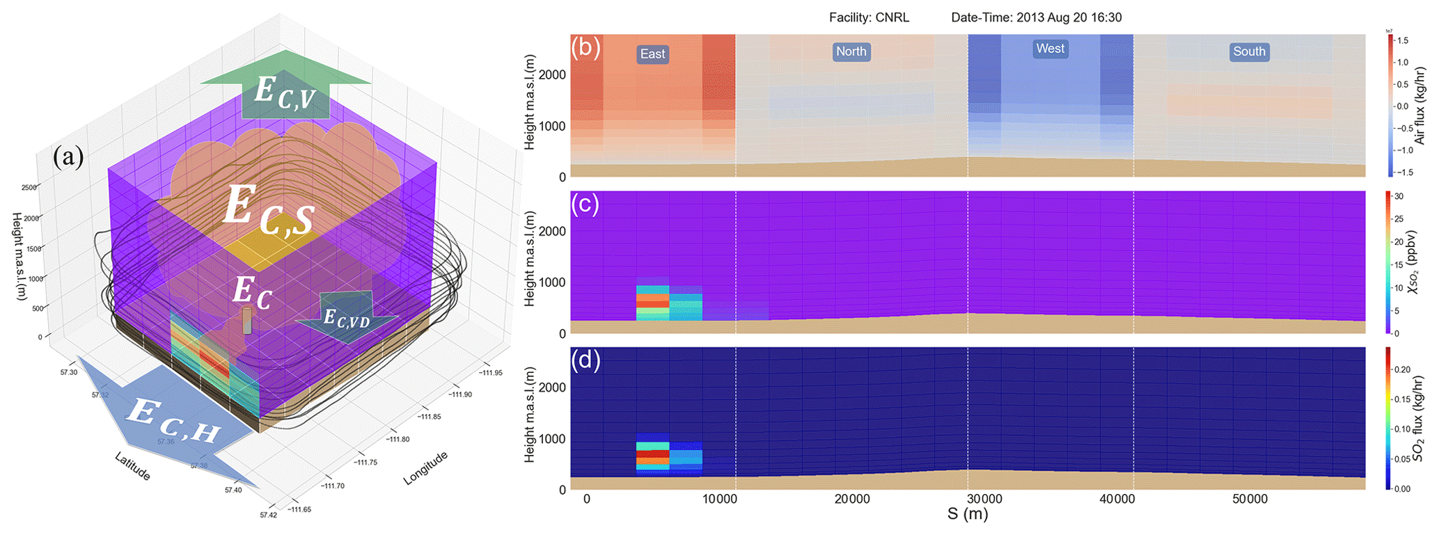
Figure 2SO2 mixing ratio screen around CNRL extracted from the GEM-MACH model output at the start of case 4 on 20 August 2013 at 16:30 UT (10:30 LT). (a) Mixing ratio data (2D) on the lateral walls of the flux box, along with the flight tracks plotted as dark dots. The additional graphics (arrows and plumes) on (a) represent processes contributing to change in tracer mass within the box volume: source emission rate (EC), horizontal flux (EC,H), vertical flux (EC,V), surface deposition (EC,VD) and storage rate (EC,S). The extracted fields around the box are unwrapped onto a 2D screen comprised of box lateral walls (east, north, west and south) and shown in (b) the normal air flux (positive outwards), (c) SO2 mixing ratio and (d) SO2 mass flux through the screen. Note that the net flux on box corners is the vector sum of the fluxes in west–east (U) and south–north (V) directions.
2.2.2 TERRA retrieval (TR) approximation using GEM-MACH 2D fields
Aircraft-based retrieval methods such as TERRA rely on measured data along the lateral walls of the box. In observation-based retrievals, the horizontal flux EC,H can be calculated (directly) from aircraft collected data and the other terms need to be estimated based on several assumptions about the atmospheric conditions and source properties (Gordon et al., 2015). Here, we explore the use of regional (GEM-MACH) model output in a similar fashion as aircraft observations, restricting our analysis to model output sampled along the lateral walls of a box enclosing an emitting facility within the model domain (GEM-MACH 2D fields). Figure 2a shows model simulated SO2 concentrations (normalized to the maximum concentration) on the lateral walls of the flux box surrounding the CNRL facility (case 4). Flight tracks on 20 August 2013 (JOSM) are also plotted as dark dots around the facility, for reference. For emissions retrieval applications using aircraft observations, the sampled observations must be interpolated (e.g., kriging) between successive circuits around the box and extrapolated to the ground surface in order for emissions to be estimated. Surface deposition rate EC,VD is also estimated using the extrapolated species mixing ratio data at the ground level. Gordon et al. (2015) estimated the uncertainty due to extrapolation of aircraft data to the ground surface as 0.4 and 12 % in TERRA estimates for SO2 plumes. Here we avoid the uncertainties arising from such assumptions by extracting model data along box lateral walls from the ground surface up to the box top, and by using GEM-MACH model surface deposition (EC,VD) values in our calculations.
For this portion of our analysis, in which we limit the inputs to mass-balance estimations to the information available on the box lateral walls in analogy to aircraft observations, instantaneous 2D screens of relevant fields (e.g., SO2 concentrations) covering the entire area comprised of box lateral walls (as shown in Fig. 2) were extracted/generated from the GEM-MACH model output at every model time step. Such screens were also generated from GEM-MACH output for air flux, based on the extracted air density ρair, the calculated normal wind U⟂ (positive outwards), and SO2 mass flux, based on concentration and air flux screens (Fig. 2b–d). The integrated horizontal flux through the screen EC,H was then calculated using Eq. (B1). In observation-based applications, TERRA estimates the changes in mass due to variations in air density over flight time, Eair,M and EC,M, based on observed meteorological trends in air density () from nearby weather stations (towers) and average species mixing ratios (χC) around the box. Here, we substituted the weather data with a single column (GEM-MACH-predicted) air density temporal rate of change at point (xo, yo) located at the horizontal center of the box for each of the nine studied cases. Here, single column is assumed to represent the spatial average rate of change in air density over the region of interest through the assumption of horizontal homogeneity, as in observational TERRA applications. Our comparisons between the GEM-MACH box average and the single column rate of change in air density indicate <5 % difference between the two trends for the time periods of our studied cases. This gives
where A is the base area of the box. is the average GEM-MACH-predicted species mixing ratio around the box along the flight path (s) at height z, which is the same as in aircraft-based applications of TERRA.
Furthermore, due to lack of measurements at the box top, the vertical flux EC,V in TERRA in observation-based applications is estimated in two steps: (a) the vertical air mass flux (EC,V) is estimated based on the other terms by rearranging the mass balance expression for air (Eq. 8), and (b) the species mixing ratio (e.g., SO2) at the box top is assumed to be uniform and equal to the average (along flight path s) screen top mixing ratio () (Gordon et al., 2015). Here, the same procedure was employed in deriving the vertical flux through box top using GEM-MACH output fields,
As there are no volumetric data available in aircraft measurement applications of TERRA, the storage rate within the box cannot be inferred directly. Emission rate estimations in aircraft-based methods such as TERRA are made with the underlying assumption of steady-state conditions and therefore EC,S is assumed to be negligible, effectively incorporating it into (the superscript “tr” referrers to TR method estimates). Thus, for aircraft-observation TERRA applications, mimicked here, Eq. (7) is reduced to
Estimations of emission rates were made for each model time step (using instantaneous 2D screens) during the time periods of the nine studied JOSM cases by using GEM-MACH output to approximate the input data for TRs as described above. Note that the TR method, as described in this section, makes use of GEM-MACH 2D data at each time t to generate an estimate (one estimate at each time step t during the entire sampling period) while making approximate estimations of the temporal gradient terms (Eqs. 9 and 10) at time t by following procedures similar to aircraft-based applications of TERRA. Flight-time-averaged estimates are then compared to the flight-time-averaged MIEs (Sect. 3.2).
2.2.3 Revised TERRA retrieval (TR*) using GEM-MACH 3D fields
Utilizing time-consecutive instantaneous screens around an emission source, the temporal evolution of the system and its impact on mass-balance estimates can be studied in more detail, as discussed at the beginning of this section (Sect. 2.2). By using air density screens at every 2 min model time step (2D space, 1D time), as opposed to using a single column (vertical) profile in the TR method, estimations of Eair,M and EC,M can be improved (by 1 %–3 %, determined through comparisons with GEM-MACH box averaged temporal trends):
where and are the average GEM-MACH-predicted air density and species mixing ratio around the box (along s) at height z. A similar procedure (using time-consecutive screens) can be used for estimating the storage term EC,S. The main difference between DR (Eq. 7) and TR (Eq. 12) retrievals is that the former explicitly accounts for and calculates the storage term EC,S. As discussed later in Sect. 3.3, the results from the direct retrieval (DR) method demonstrate the potentially significant contribution of the storage term EC,S to the total integrated estimated emission rates EC (Eq. 7). Ignoring this term, as in Eq. (12), could result in substantial over-/under-estimates, if retrievals are attempted for conditions where the underlying assumption of time-invariant meteorology is not met and/or when significant upwind emissions (from other sources) enter the flux box. As noted in the Introduction, a priori metrics may be used to avoid these conditions. The key information for calculating EC,S, is the estimate of the temporal gradient in species mixing ratio () as in Eq. (4). This is achieved in the DR method by utilizing GEM-MACH model 4D data (volumetric time series) and integration over the entire volume of the box at each model time step. These 4D data are not available for aircraft applications of retrieval algorithms, since instantaneous datasets cannot be created from flight information, and collection of volumetric data may not be operationally feasible in aircraft campaigns, where flight durations may be limited to a few hours. However, data from time-consecutive 2D screens may be used to approximate EC,S, leading to improved estimates of emission rates – by providing ancillary information for the study of temporal trends in chemical and meteorological fields. As we show later in Sect. 3.3, estimates of the storage term from time-consecutive 2D screens () are strongly correlated (Pr=0.9) with the corresponding DR estimates of EC,S using volumetric (3D) time series. This high correlation suggests that EC,S can be approximated using generated from time-consecutive 2D screens (3D fields) as representative of the rate of change in mass within the volume of the box. The approximation of EC,S using screen data alone is given by
where, same as in Eq. (14), and are the average GEM-MACH-predicted air density and species mixing ratio along s (around the box) at height z. Note that the key difference between Eqs. (4) and (15) is that the former integrates over the volume, using consecutive time steps of chemical transport model output, while the latter integrates over average values along s at each height level z on the screen walls using consecutive time steps, and multiplies the result by the box horizontal area. However, Eq. (15) may also be generated from observations, something which is not possible for Eq. (4). For the case of aircraft observations, a repeat flight would be required: rather than just a single flight path starting near the surface and working upwards along the box boundary, the aircraft would execute (at least) two consecutive box flights around the same facility. A better approach would be the use of two (multiple) aircrafts, or UAVs as they are becoming more popular for air-quality measurements (e.g., Elston et al., 2015; Mölders et al., 2015; Barchyn et al., 2018; Li et al., 2018), flying in tandem following the same flight path in order to reduce time lag between samplings (in turn reducing the chance for meteorological variability to be a concern). Differencing between the fields obtained from consecutive flights would be used to estimate the value of . As we discuss below, the use of either ground-based or airborne remote sensing is another potential means to estimate . The correlation between EC,S and also indicates that the latter may be used to estimate, from repeat flight aircraft observations and/or remote sensing, the extent to which within-box mass storage may influence emission rate retrievals.
Considering the potentially prohibitive operational cost of conducting repeat flights and the fact that few (e.g., two to three) time-consecutive measurements may not provide enough information for the estimate of temporal trends in within-box tracer mass budget, the following alternative is proposed. As we discuss later in Sect. 3.3, observed temporal trends of tracer concentrations () downwind of the emission source are also in similar strong correlation (Pr=0.9) with the corresponding DR estimates (using volumetric time series). Furthermore, our studied cases suggest that downwind vertical profiling of tracer concentrations can provide similar estimates of the temporal tends required for the estimate of the storage rate and can be substituted in Eq. (15) for . In observational applications, this can be achieved through ground-based or, preferably, aircraft-based vertical profiling remote measurements (e.g., lidar measurements, Aggarwal et al., 2018), where the sampling aircraft with a remote measurement setup would collect column data while flying around or downwind of the emission source. The use of an aircraft-based vertical profiling instrument for a small number of chemical fields, along with a repeated, single-loop flight path around a facility (10–15 min) would generate fields similar to those generated by the air-quality model used here, in turn allowing highly time-resolved estimates of the storage term. This alternative approach can be more cost (operational) efficient compared to the strategy of repeat flights (which would require a second aircraft traveling in tandem behind the first to achieve the same time resolution) while providing more time-consecutive data points for the study of the temporal trends in the tracer mass budget and further reducing the relatively small emissions biases associated with extrapolation to the ground of observed fields.
We note that the correlation between EC,S and was deduced here through GEM-MACH model simulations with model grid point resolution (in the horizontal) of 2.5 km. This correlation (and the corresponding time/length scales) can be further investigated through model simulations at higher resolutions (e.g., 50–250 m) and/or field observations (e.g., controlled tracer release). Equations (14) and (15) along with the other terms in Eq. (12), give the TR* method,
Using the consecutive screens at every model time step (extracted from GEM-MACH model output fields), estimations of and were made for the period of the nine JOSM 2013 cases around Syncrude, CNRL and Suncor facilities. Retrieved emissions by the TR* method (where tr* refers to TR* and tr to TR method estimates) were compared to the MIEs as well as to the estimations made with the DR and TR methods (EC and , respectively).
Table 1 summarizes the main features of the three retrieval methods (DR, TR and TR*), along with possible practical/observational applications for each. Meta-data-set types, terms for estimating the source emission rates, descriptions for each method, and their relevant equation numbers are also noted on the table. The horizontal flux and deposition terms EC,H, EC,VD are shared among all three methods, with the other terms approximated for the TR and TR* methods. Note that here EC,VD is “directly” extracted from the model output, but in observational methods this term is also approximated based on the other measured fields (Table 1). Results and discussions follow.

Figure 3 summarizes the retrieved emissions by the three methods (DR, TR and TR*) and their performance against the MIEs; vertical lines represent the over-/under-estimates by the TR method due to the exclusion of the storage term (EC,S) in Eq. (12), for each case. Also shown in Fig. 3 for reference are the ±50 %, 30 % and 20 % error limits, with ±30 % corresponding to the maximum estimated uncertainty for TERRA applications in Gordon et al. (2015). Estimates for most of the flight cases studied here using GEM-MACH output fell within ±30 % of MIEs, exceptions being cases on 26 and 28 August (cases 5 and 8). The latter two flights were not analyzed in past work due to unfavorable conditions for reliable application of TERRA, namely, light variable winds (case 5) and high upwind emissions (case 8). However, they have been included here using GEM-MACH predictions in mass-balance estimates, as extreme cases in which storage-and-release events have a significant influence on resulting retrievals. We herein refer to cases 5 and 8 as the rejected cases. Using the DR method, we were able to determine the relative contribution of the different terms to the net estimate of EC (Fig. 4).
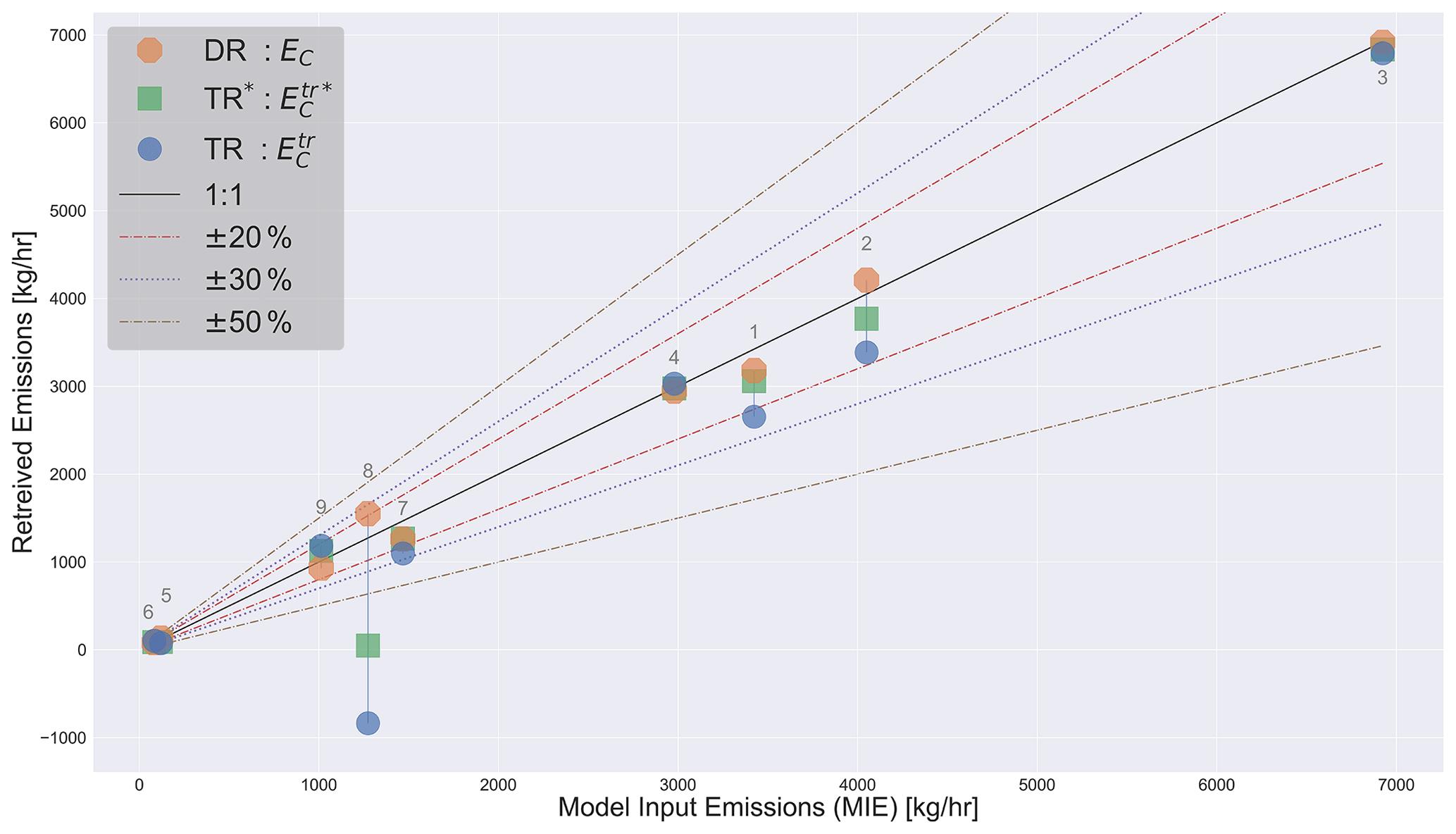
Figure 3Emission rates determined by the three methods (DR, TR and TR*) are plotted against model input emissions (MIEs). The dark solid curve is the 1:1 MIE line; estimates below and above this line represent under- and over-estimation by the three methods. Case IDs are noted for each set. The vertical lines represent the error associated with storage-release events (EC,S) in TR estimates relative to MIEs. Also shown in the figure are the ±50 %, 30 % and 20 % error limits (dashed lines) for reference.
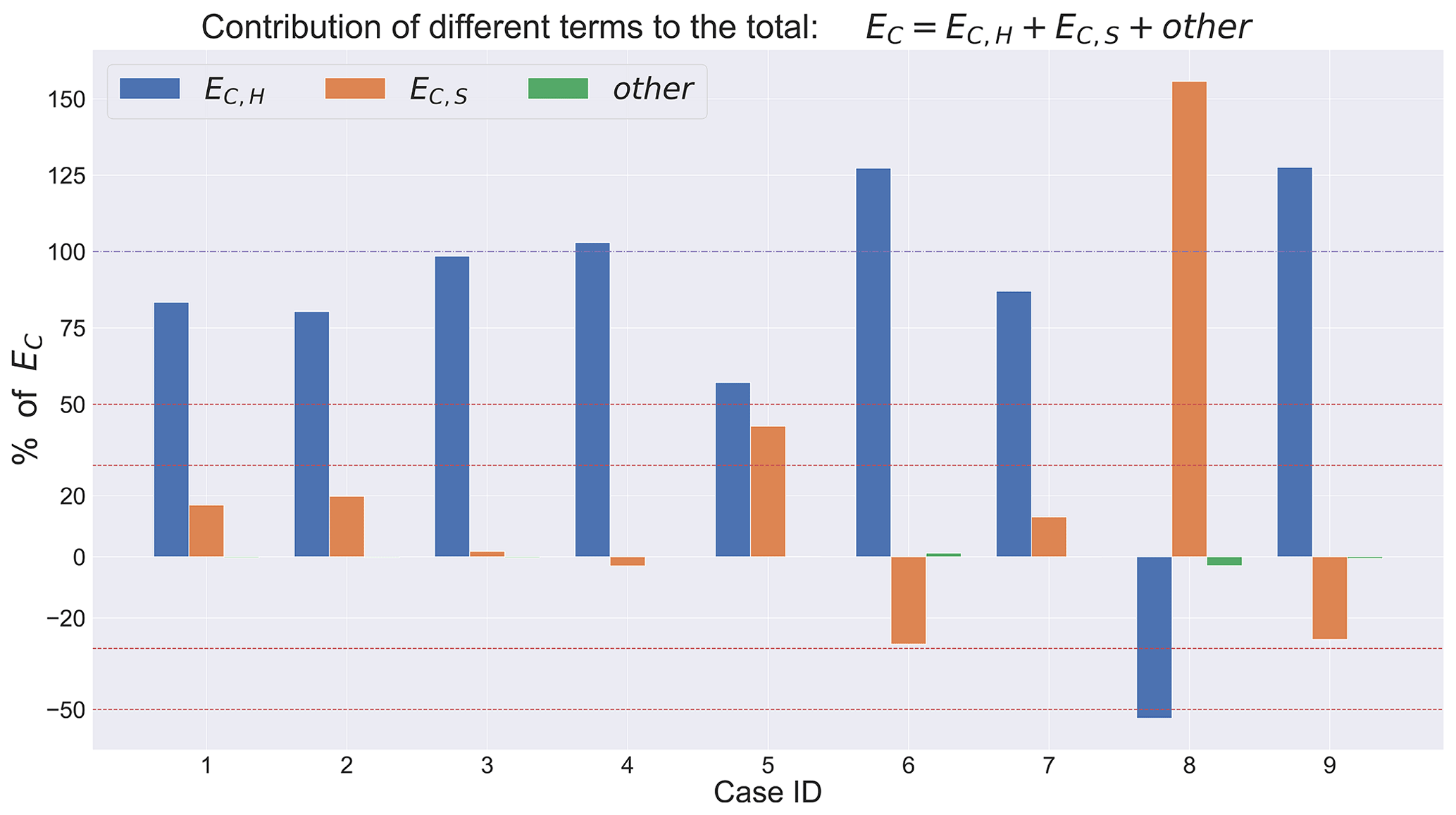
Figure 4Contribution (%) of different terms in Eq. (7) to the total retrieved emissions (EC), for the nine JOSM 2013 cases. The 100 % contribution level is marked with a (purple) dot-dashed line, ±30 % and 50 % levels are also marked with (red) dashed lines on the figure. The main contributing terms were EC,H and EC,S (>97 %). The other terms contributed <3 % combined.
3.1 DR
DR estimations were made by analyzing model 4D data for flux boxes approximating the nine cases. The numerical integration expressions for calculating each term, using model data, are described in Table B1. Estimates of EC for SO2 emission rates for the three oil sands facilities (Syncrude, CNRL and Suncor) were made by substituting the calculated terms from Table B1 in Eq. (7). Figure 4 demonstrates the contribution of each of the terms in Eq. (7) to the total integrated emission rate EC by DR from the GEM-MACH model 4D data for the nine flight cases. As shown in Fig. 4 the main contribution came from two terms, the net integrated horizontal flux EC,H and the storage term EC,S, together contributing >97 % of the net change in mass. For seven out of nine studied cases, EC,H accounted for >80 % of the total emissions (EC). This is in agreement with another model-based study by Panitz et al. (2002), where the contribution of advective fluxes (EC,H and EC,V) were estimated as 85 % and 95 % with no estimation of the storage term. The combined contribution of the other terms (EC,V, EC,VD and EC,M) were <1 % for all cases except for cases 6 and 8 (2 September and 28 August) were it was 1.2 % and 2.9 %, respectively. For two out of nine studied cases, the contribution of the storage term (EC,S) was >30 %, the maximum estimated uncertainty for cases analyzed in Gordon et al. (2015). As discussed earlier, these flights were not analyzed in past work –- but they have been included here as good examples of cases in which time-variant meteorology and/or high upwind emissions result in significant over-/under-estimates due to storage-and-release events. We also show later in Sect. 3.3 how these estimates may be improved.
DR method estimates were compared to the MIEs, as shown in Figs. 3 and 5 and Table 3. Estimates were within 1 %–23 % of MIEs for the nine studied cases. We note that in some cases (4, 6 and 9), negative EC,S values reduced the net EC estimate. Rejected cases 5 and 8 were the two cases with the largest storage term (EC,S) contributions of 43 % and 156 % (averaged over flight time) of the total estimated emissions (EC), respectively. Once corrected for storage (i.e., DR method), estimates for these two cases were within 12 % and 23 % of MIEs. Cases 3 and 4 had the lowest storage rates (2 % and −3 %), where storage-corrected estimates were within 1 % and 2 % of MIEs, respectively.

Figure 5Time series of the estimates by DR, TR and TR* methods, plotted along with MIEs. Normalized-root-mean-square (NRMS) error for the three methods are noted on the plot for each of the nine JOSM 2013 cases. JOSM 2013 flights on 24 August (case 2) and 2 September (case 6) included two consecutive box flights around the same facility, shown as shaded areas on their respective time-series plots. Note that the DR and TR* methods, unlike the TR method, account for the storage rate (EC,S and ).
For the majority of our studied cases, our results indicate that the storage term (if not accounted for) contributes the bulk of emission rate over-/under-estimates for the variables investigated here, and hence methods to predict and/or reduce its influence are desirable for aircraft retrieval algorithms. We note that the impact of storage on emissions retrieval estimates will depend on the relative magnitude of the estimated emissions themselves in comparison to other sources of uncertainty. That is, an emissions estimate double that of previous estimates, which has a ±30 % over- or under-estimate associated with storage, may still be concluded as being significantly higher than the previous estimates (i.e., the emissions change is greater than the uncertainty associated with the retrieval itself). However, the storage term as defined here has been shown to be the main contributor to emissions over-/under-estimates, and will therefore be examined in more detail in the analysis which follows. We also note that the impact of EC,S is sometimes negative, a net release of mass from the box. Note that net releases of stored mass from the box would result in emissions over-estimates; net storage of mass within the box would result in emissions under-estimates.
Storage-and-release events occur when mass is accumulated within the volume of the box and released at a later time through box lateral walls; see the detailed discussions in Sect. 4. Such events can be detected on the box walls by comparing the temporal variation in the net horizontal flux, EC,H with EC,S. Figure 7c and d (Sect. 4.1) show time series of the horizontal flux EC,H and the storage rate EC,S for case 4 on 20 August 2013 (CNRL). Storage-and-release events are represented by peaks and troughs in the EC,S curve, which coincide with troughs and peaks in the EC,H curve. EC,H and EC,S are anti-correlated (with Pearson correlation coefficient of ) for case 4. Pr values between EC,H and EC,S were in the range −0.68 to −0.98 for the nine cases, indicating strong anti-correlations for all the studied cases. Positive values of EC,S correspond to storage, which result in decreased net flux exiting through the box walls; negative values correspond to release, which results in increased net flux exiting through the box walls. Therefore, temporal variations in EC,H over the period of a flight around an emission source with relatively constant emission rates, can be attributed to mass storage/release. This provides a potential practical means for detecting storage-release events in aircraft-based retrieval methods as the horizontal flux (EC,H) can be calculated directly using airborne measurements along the box lateral walls, if ancillary information is available, such as from repeated flights. Changes to the calculated EC,H can indicate the potential presence of storage-and-release events within emissions observation data collection time periods.
3.2 TR
By limiting the analysis to the extracted model data along box lateral walls (Fig. 2), TR estimates of MIEs were made. Terms in Eq. (12) were solved numerically using model data, with EC,H calculated as described in Table B1; numerical expressions for calculating the rest of the terms are described in Table B2. Model surface deposition rates for the base area of the box (A) were used in TR estimations, similar to the DR method, the main difference between these two methods is that, unlike Eq. (7), Eq. (12) does not account for the storage term. TR estimates of SO2 emission rates were within 4 %–39 % of MIEs for eight out of nine studied cases; see Table 3. For cases 3 and 4, the two cases with the lowest net storage, results were within 4 %–6 % of MIEs. For the rejected case 8 with the extreme storage event, the TR method under-estimated the model input emissions by −166 %; during the sampling period of this case, on average ∼1.5 times more SO2 mass entered the flux box through the upwind wall than left through the downwind wall.
Comparing the performance of the two methods (DR and TR) against MIEs reveals the significance of the storage term (EC,S) in emission rate retrievals. Figure 5 shows the time series of retrieved emissions using the DR and TR methods for the nine cases, with model time-step temporal resolution (Δt=2 min). MIE time series are also plotted for SO2 emissions from all the sources within each facility. Note that in aircraft-based applications of TERRA, a single emission rate estimate (temporal average) is generated based on the observations during the entire flight-time (∼2 h). Here, where we approximated the TERRA retrievals by the TR method (see Sect. 2.2.2), instantaneous 2D screen fields (extracted from the GEM-MACH model output) were used to generate an emission rate estimate at each time step using the TR method. The flight-time average estimates by the DR and TR methods were compared to the flight-time average MIE; normalized root mean square (NRMS) error scores are noted for each method in Fig. 5.
By combining the information from Figs. 4 and 5, TR estimates for the nine cases can be categorized in three groups: (a) net positive storage (resulting in emission rates under-estimation), (b) net negative storage (i.e., release of stored mass from the box during the time period studied, resulting in emission rates over-estimation), and (c) low storage amounts, the best emission rate estimates. The first group (a) includes cases 1, 2, 5, 7 and 8. For these cases the net storage was positive, where 13 %–156 % of the emitted SO2 mass was accumulated within the box volume and was not released through box walls during the sampling time. The stored mass was accumulated within the box either before or during the sampling time, which in turn resulted in decreased flux through box walls and the consequent under-estimation in TR estimations. Cases 6 and 9 fall into group (b) where the previously stored mass was released (−29 % and −27 %) through the box walls along with the SO2 mass from emission sources during the flight time, resulting in TR method over-estimation. Group (c) include the ideal cases 3 and 4 where TR estimates were within 4 % and 6 % of MIE, respectively. These two cases captured consecutive storage-release pairs over the sampling period (see Sect. 4.1, Fig. 7c and d for case 4) that canceled each other out and therefore resulted in relatively low (sampling time average) storage rates (EC,S) of 2 % and −3 %, respectively.
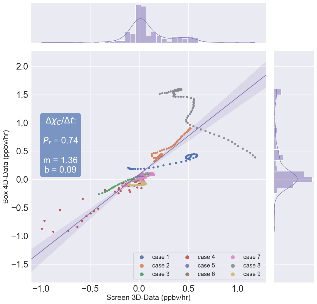
Figure 6This three-panel graph demonstrates the correlation between estimates of by analyzing 4D (box) and 3D (consecutive screens) data sets. The vertical side plot shows the range and distribution of estimates for the period of nine studied flights by 4D analysis, the horizontal side plot shows the same for 3D analysis. The main panel demonstrates the correlation between the two methods of estimation. Pearson correlation coefficient (Pr=0.74) shows the strength of this relation. The least-squares fit line has slope m=1.36 and intercept b=0.09. Note that case 8 estimates are in low correlation due to relatively high upwind emissions during the time of that particular flight case (28 August), rendering the 3D estimates less representative of the 4D estimates. Excluding case 8 from this analysis, results in Pr=0.88, m=1.07 and b=0.03. can be estimated from multiple consecutive 2D screens, by assuming 3D estimations of as representative of the rate of change in species mass within the flux box. The same can also be estimated from downwind vertical profiling of tracer concentrations over the sampling time.
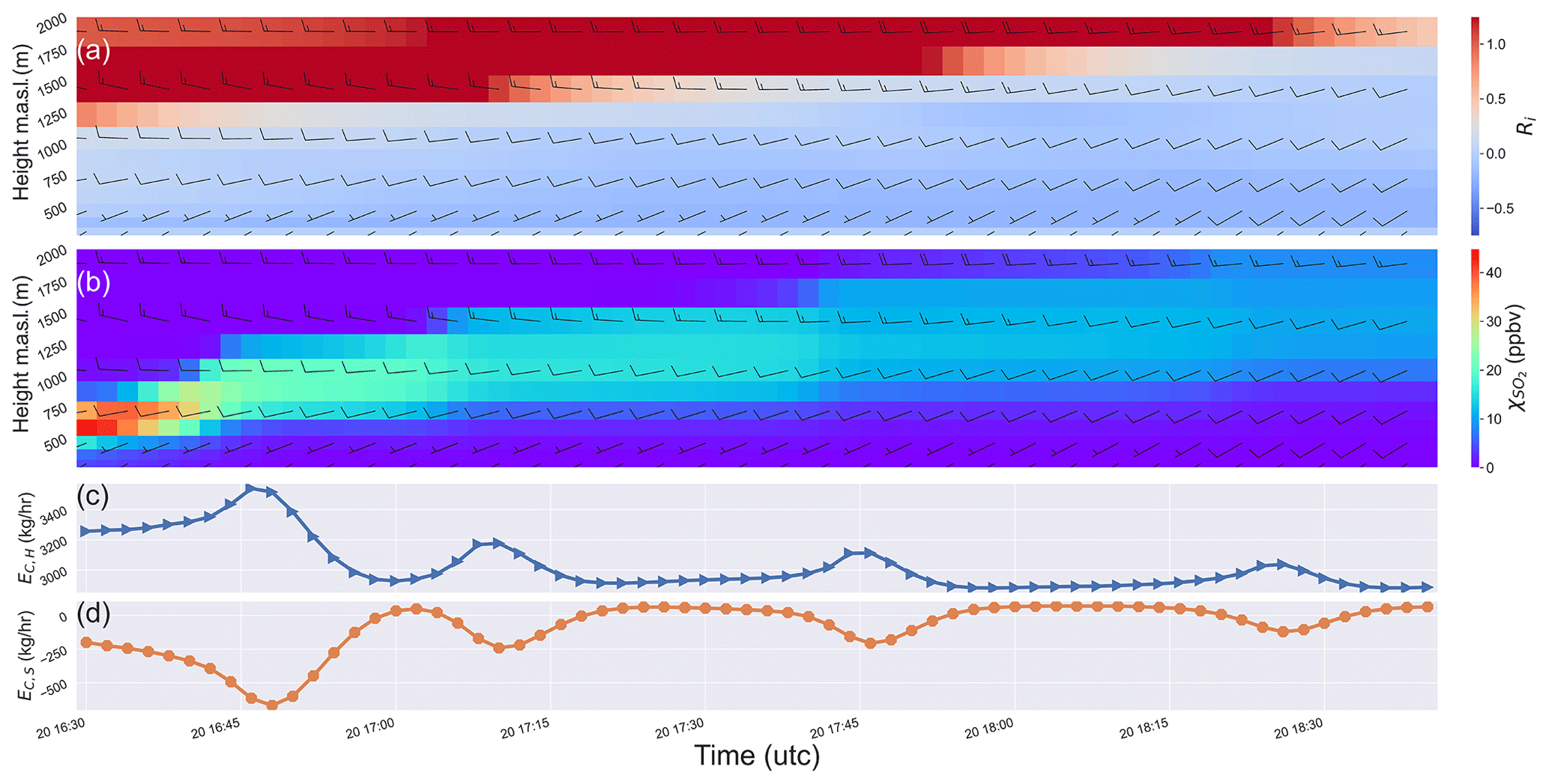
Figure 7This schematic demonstrates (qualitatively) the correlation between change in atmospheric stability represented by the gradient Richardson number (Ri), plume vertical motion and storage-release events for the period of case 4. (a) Ri vertical profiles at stack location over the flight time, with the color-scale symmetric around the critical gradient Richardson number RiC=0.25. (b) SO2 mixing ratio vertical profiles at stack location. (c) Time series of net horizontal flux (EC,H) and (d) the storage rate (EC,S), over sampling time. Note the level of anti-correlation between EC,H and EC,S (); oscillations in storage and release are occurring: changes in EC,S are matched by opposite changes in EC,H. Wind speed and direction are shown as barb plots with units m s−1 (half = 5, full = 10). For every incremental rise in plume height, a corresponding release event occurs. As the plume ascends into regions with faster wind speeds, more mass is released () through the lateral walls resulting in an increase in EC,H as can be seen in (c).
3.3 TR*
Here we show that change in tracer mass within the flux box can also be observed on box lateral walls over time (using time-consecutive screens), as described in Sect. 2.2.3. Figure 6 demonstrates the correlation between the 4D (volume) and 3D (screens) estimates of the temporal change in species mixing ratio () for all the data points (2 min resolution) corresponding to the period of the nine studied cases. The side plots show the range (and distribution) of the estimated by 3D (horizontal axis) and 4D (vertical axis) calculations. The range is slightly higher for 4D estimates (2.52 ppbv h−1) than for 3D estimates (2.17 ppbv h−1), and the two variables are strongly correlated. The correlation coefficient Pr=0.7 (with slope m=1.36 and b=0.09 intercept for the least-square fit line), indicates strong correlation between 4D and 3D estimates. An exception is rejected case 8, where the correlation is low due to relatively high upwind emissions during the time period of this case (on 28 August). Excluding case 8 from this analysis, increases the correlation between 3D and 4D estimates to Pr=0.9 (with m=1.07 and b=0.03). As discussed earlier, the lack of information about the storage rate was the primary source of under-/over-estimates in TR method estimates for the majority of our studied cases. Here we demonstrate the use of an estimate of the storage term (; see Sect. 2.2.3) in a revised retrieval approach. We note that this term may be estimated from consecutive screens (Eq. 15) or tandem aircraft samples for ambient atmosphere applications. As discussed in Sect. 2.2.3, an alternative to multiple aircraft-based measurements is to estimate the temporal trends in tracer concentrations () through remote vertical profiling (e.g., lidar measurements). Our analysis of different flight cases show that downwind trends are also in strong correlation with DR method volumetric time-series estimates with the same correlation coefficient of Pr=0.9 (with different m=0.57 and b=0.03). The advantage of remote (downwind and upwind) vertical profiling over multiple aircraft or UAV measurements, in addition to operational cost efficiency, would be the collection of more temporal measurements over the sampling time, which in turn can result in improved estimates of and the storage term (), as opposed to estimates based on a few time-consecutive measurements (e.g., two to three) via multiple or in tandem aircrafts. Data from time-consecutive screens/measurements can then be used to numerically solve Eqs. (14) and (15) (see Table B3 for discrete integral expressions). For GEM-MACH-driven retrievals as used here, these time-consecutive screens originate from consecutive model output times. Here, we show the effect of the estimate on the resulting TR* emission rate estimates () using GEM-MACH fields for top-down retrievals. Improved/revised TERRA retrievals (TR*) can be made by plugging in and in Eq. (16). TR* method estimates are compared to the MIEs in Figs. 3 and 5 and Table 3. For eight out of nine cases, TR* estimates were within 2 % to 34 % of MIEs. TR* estimates showed improvement over the TR method for all the cases (including the rejected case 8) by 2 %–52 % of MIEs; see Table 3. TR* estimations rely on the availability of temporal data for estimating change in tracer concentrations () along the box lateral walls (or only on the downwind wall) for each emission rate retrieval case, which in our analysis with simulated fields were readily available with the GEM-MACH model data at each time step. Again, for observational applications: (1) a repeat box flight procedure can be used, where an aircraft carries out a second box flight immediately after the first flight, or two aircraft (or UAVs) follow the same flight path in tandem, one positioned a fixed distance behind the other, or (2) remote vertical profiling (e.g., remote lidar measurements) on a single aircraft can be employed to collect time-consecutive measurements of relevant fields, in the column, around the emitting facility.
The main processes contributing to the change in SO2 mass within the volume of the box are illustrated in Fig. 2a (EC, EC,S, EC,H, EC,V and EC,VD). An SO2 emission source continuously adds mass to the box at emission rate EC. Most of the mass is advected out of the box through the top and lateral walls (EC,V and EC,H), and some is deposited to the ground surface (EC,VD). All the while, mass is continuously stored within the volume of the box and may later be released at net storage rate EC,S (positive to negative). Under time-invariant conditions (e.g., wind field, atmospheric stability, emission rate), the rate of generation of mass (EC) is at net (mass) balance with the other mass-removing processes (EC,H, EC,V and EC,VD) and the total accumulated mass within the box volume (BC) remains relatively constant over time, and the storage rate negligible (). The mass-balance approach based on the divergence theorem (Eq. 12) can therefore accurately equate the source emission rate to the net integrated flux leaving the box through the enclosing surfaces. However, localized (spatial) variations in meteorological fields (e.g., atmospheric stability, wind) and chemical fields (e.g., temporal changes in source emission rate (EC) and/or significant incoming upwind emissions) during the retrieval time, can shift the mass balance towards (Eq. 7) – i.e., storage-and-release events. The scale and duration of the storage-and-release events contribute to over- and under-predictions in estimated emissions based on the mass-balance approach. Using GEM-MACH model 4D data we carried out extensive analysis of the storage-release events during our studied cases and devised three quantitative predictors for the severity of these events. In the following subsections, using results from DR, TR and TR* estimates, we discuss these parameters and their correlation with over- and under-estimates in top-down mass balance emission rate retrievals due to storage-and-release events.
4.1 Gradient Richardson number (Ri) and changing atmospheric stability
Aircraft-based emissions retrieval methods such as TERRA, utilize the mass-balance approach with the underlying assumption of mean steady-state conditions over the region of study ( km2) during the flight time (∼2–3 h). However, localized and transient variations in atmospheric stability at the vicinity of the stack/source location can impact the pollutant plume rise and transport within the box and result in storage-release events. Horizontal wind velocity usually increases logarithmically with height. The height the plumes reach in the atmosphere depend on the stack parameters (exit velocity, exit temperature, stack height) and on the local stability conditions (temperature and wind profile near the stack location). Thus plume height may change with varying stack parameters and stability conditions during the course of a retrieval. This in turn would move the mass to a different flow regime – e.g., higher horizontal velocities if the plume height has increased, and lower horizontal velocities if the plume height has decreased. These changes in plume height, in response to changes in atmospheric stability, may thus lead to a change in the rate at which emitted mass is transported out of the box. Stability changes are thus a good predictor of the possibility for mass storage and release. A measure of the change in dynamic stability is therefore desirable as a predictor for conditions under which this aspect of the “static meteorology” condition, required for reliable top-down emission rate retrievals, is not met.
Atmospheric dynamic stability can be described in terms of the gradient Richardson number (Ri), which is a dimensionless ratio, related to static stability and the shear induced turbulence (American Meteorological Society – AMS, 2021a),
where θv and Tv are virtual potential temperature and virtual absolute temperature, respectively, g is the gravitational constant and U and V are the horizontal wind components. The sign of Ri is determined by the static instability term () in Eq. (17); the denominator is always positive. In the presence of a strong wind shear Ri approaches 0. The critical gradient Richardson number (Ric) is about 0.25, below this value the atmosphere is dynamically unstable. The atmospheric Physics module within the GEM model includes the estimation of atmospheric stability and calculations of the gradient Richardson number, Ri (Mailhot and Benoit, 1982), which is also used as a parameter (in addition to emission stack/source information such as temperature, exit velocity) to calculate plume rise height (Akingunola et al., 2018). Changes in Ri with respect to time are thus an indicator of the potential for the plume to change height during an aircraft emission rates retrieval; Ri may be predicted using a weather forecast model as part of pre-flight planning.
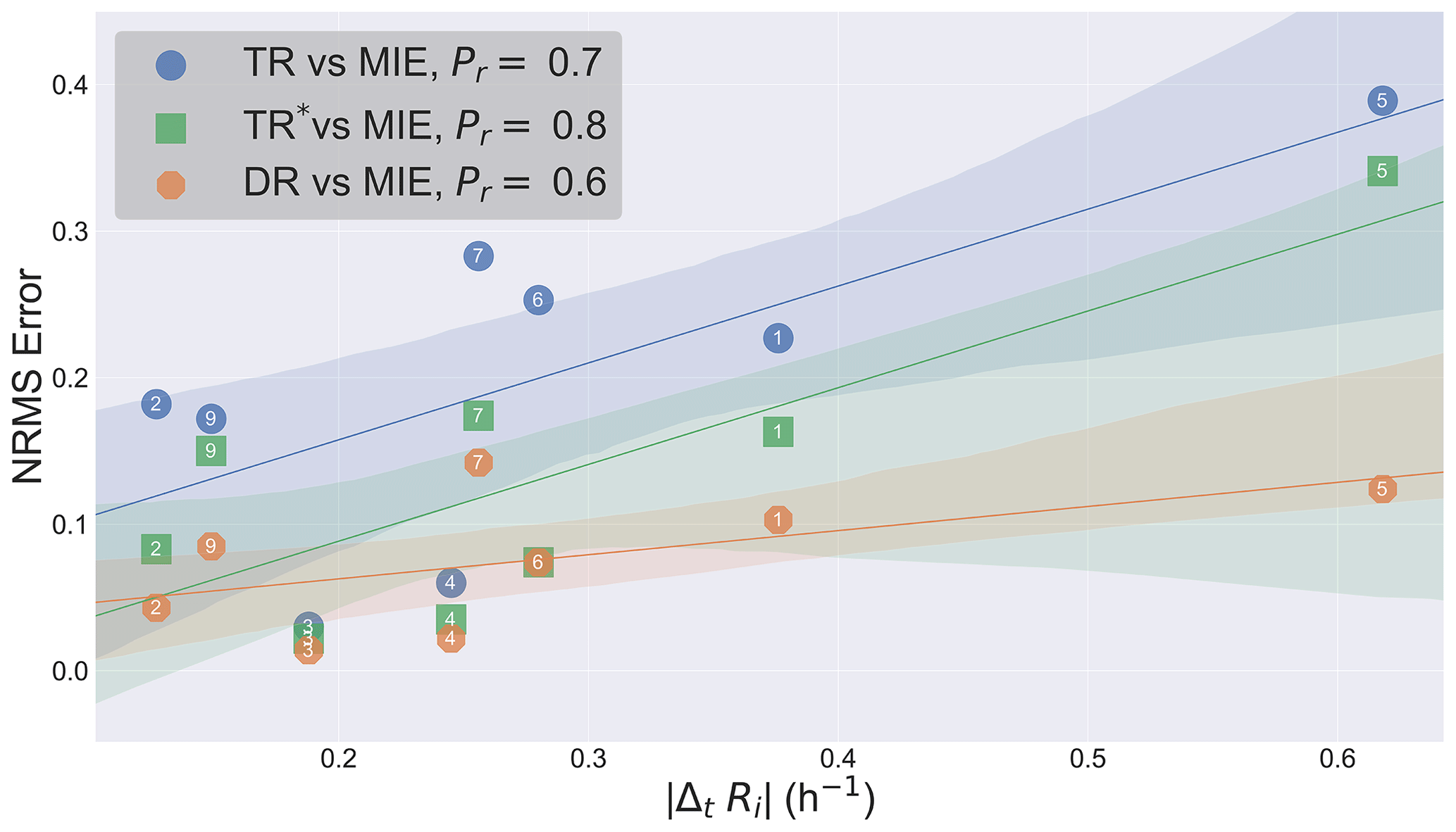
Figure 8Correlation between the NRMS error and the change in atmospheric stability represented by the absolute change in the gradient Richardson number . The shaded areas indicate the 90 % confidence region. Case ID is indicated for each data point on the graph along with the calculated Pearson correlation coefficients (Pr) for the three methods. Results indicate a strong positive correlation between the NRMS error and .
For our analysis, 4D fields of Ri were extracted from the model output dataset for each of the nine studied cases. Figure 7 shows the case for the JOSM flight on 20 August (case 4) with vertical profile time series at the location of the emitting stack, and compares Ri in (a), with the SO2 mixing ratio in (b), the net horizontal flux EC,H in (c) and the storage rate EC,S in (d). As shown in Fig. 7a, the region of unstable air (blue) was gradually increasing in height during the sampling time, resulting in an increase in the vertical extent of the mixing layer. Note that the color-scale is symmetric around the critical gradient Richardson number RiC=0.25 in Fig. 7a. The increase in the vertical extent of the mixing layer during the period of case 4, resulted in the SO2 plume mixing into heights with higher wind speeds (Fig. 7b). The incremental plume rise resulted in a sequence of fast-release events, that is, the simulated plume was moved into a faster (higher level) horizontal flow, and SO2 mass was carried to the boundaries of the box faster – the net rate of mass loss through the downwind walls thus increased during the sampling time period (, Fig. 7c; , Fig. 7d). Note the anti-correlation between EC,S and EC,H in Fig. 7c and d. We also note that although faster moving flow can result in more mixing and the subsequent plume dilution, the decrease in compound mixing ratio is not necessarily enough to compensate for the increased exiting flux. If emissions retrievals are calculated under these conditions without accounting for the storage term (negative in this case), emissions estimates will be biased high (over-estimation). These fast-release events temporarily disturb the required balance between the addition of mass to the box volume by source emissions (EC) and removal of the mass through vertical and horizontal fluxes and surface deposition, causing a negative change in the total stored mass (BC) within the volume of the box (). These release events can be seen as troughs (peaks) in the EC,S (EC,H) time-series plot (Fig. 7c and d). While the plume remained at a constant height, the balance was restored over time (); this can be seen as peaks/plateaus in EC,S time series in Fig. 7d. After these periods of changing stability, the plume started to rise again, and the balance was shifted, again resulting in negative EC,S values. This process was repeated several times over the period of case 4, resulting in a sequence of release events. Note that the trough to peak duration (period) and scale (magnitude) of each event are inversely proportional to the wind speed at plume height, and they are reduced as the plume ascends into faster moving layers of air resulting in a damped oscillatory storage and release sequence. In this particular example, this periodic storage release during the sampling time, with subsequent equilibrium intervals, resulted in relatively small net storage of % over the sampling time and TR estimates within 6 % of MIEs (slight over-estimation) for case 4. When consecutive storage-release pairs are captured during the flight/sampling time as in case 4, the average error due to storage term (EC,S) is reduced. However, if the storage or release is of longer duration, so that an unpaired event occurs during observations, the net error increases, as was the case for flight case 9 where an unpaired release event (one storage-release pair and one additional release event) resulted in net storage of % and a consequent TR over-estimate. Monotonic storage or release events occur when mass is continuously stored (e.g., when a plume descends into slower moving air throughout a sampling interval; and ) or released (e.g., release of previously stored mass during a sampling interval; and ); such events result in TR under-/over-estimates as in case 2 where net storage of % (i.e., storage event: and ) resulted in TR under-estimations.
The average value at plume height, indicates unstable conditions (Ri<RiC) during the period of case 4 – the average value was calculated by spatially averaging Ri at the vertical layer containing the plume center (maximum concentration in the vertical) over the horizontal extent of the box at each time step and then averaging over the sampling time. Atmospheric stability was further decreased at an average rate of h−1 over the period of this case. Change in atmospheric stability (represented by ΔtRi) is thus related to plume vertical motion and mixing, which in turn contributes to storage-release events and a corresponding over- or under-estimate in TR retrievals; ΔtRi is thus a useful forecast metric to use as an a priori indicator of the potential for changing atmospheric stability affecting emission rates retrieval accuracy, and may also be calculated from retrieved aircraft meteorological data. Table 3 lists (flight time) average Ri and ΔtRi values for each of the nine studied cases. Our analysis indicates a strong positive correlation between the absolute value and the NRMS error for the DR, TR and TR* methods with the Pearson correlation coefficients (Pr) of 0.6, 0.7 and 0.8, respectively. Figure 8 shows the correlation between and NRMS error for each method. Note that the rejected case 8 with h−1 (see Table 3) was excluded from correlation analysis as an outlier, due to the extreme impact of high upwind emissions (and not meteorological variability) on emission rate estimates (further discussed in Sect. 4.3). ΔtRi can be calculated from aircraft-measured data along the lateral walls of the box and the measured data from additional profiling spiral flights upwind and downwind the source, such as those conducted during JOSM2013 campaign. Analysis of ΔtRi can provide insights regarding the change in atmospheric stability and the probability of plume vertical motion and the resulting storage-release events during flight time; the uncertainty levels associated with the storage rate (EC,S) in the retrieved emissions can therefore be quantified.
4.2 Plume vertical motion and variations in the direction of the transport (Δtα)
The direction of the wind experienced by the plume may change when the plume remains at one altitude, or may change as the plume rises or falls in the atmosphere (e.g., via the well-known “Ekman spiral” of wind direction changes with increasing height, AMS, 2021b). Changes in wind direction for a fixed plume height would result in the rejection (for top-down retrievals) of the flight – here we note that changes in wind direction due to plume vertical motion may also be a potential reason for flight rejection. Using GEM-MACH-predicted wind fields for the nine studied cases (chosen a priori for relatively constant wind speeds at each height), we here investigated the extent of variations in wind direction at the time-varying vertical level containing the plume center,
where σα is the standard deviation in wind direction αwind time series (spatially averaged over the horizontal extent of the box including lateral walls at each time step) and ΔtSP is the sampling period time duration. In aircraft-based retrievals (e.g., TERRA), Δtα can be estimated from aircraft measurements around the box at plume center-point height. Our analysis of the wind fields for the nine studied cases indicates a positive correlation (Pr=0.6) between the rate of variation in wind direction (Δtα) and the rate of change in atmospheric stability (ΔtRi). Variations in the direction of the flow at plume height (Δtα) can result in the re-circulation of the plume, accumulation of the emitted mass within the volume of the box and its release at a later time (storage-release event). Such an event occurred during our GEM-MACH model simulations for the period of the JOSM flight on 26 August around CNRL (case 5). Figure 9 shows horizontal cross sections of the SO2 mixing ratio data at two (consecutive) plume-maximum heights and over time for case 5. Starting from top left at 20:20 UT and height H1=909 m a.s.l. (meters above sea level) to the bottom right at 21:30 UT and height H2=1079 m a.s.l., horizontal cross sections are plotted at plume center-point (maximum concentration in the vertical) height at each time. Air flow direction and strength are shown as grey arrows on each panel. The model shows strong vertical wind shear between these two heights, with a ∼180∘ shift in the wind direction between the upper and lower rows of panels which remains relatively constant with time. This is a subtle example of how wind direction changes may interact with changes in stability: while the wind direction is relatively static at each height, changes in stability may cause the plume to rise to different heights, where the wind direction may change or even reverse relative to the level below. The changes in turn will alter (slow) the rate of mass release from the walls of the box (), a storage event, with . For this particular case (case 5), between 20:20 and 20:50 UT, the plume center was at H1 and was advected in a weak south-easterly wind; between 20:50 and 21:00 UT, the plume mixed upwards and rose to H2, where wind direction was north-north-westerly and remained there until 21:30 UT (which afterwards descended back to H1). This change in wind direction at plume height (Δtα) as a consequence of plume vertical motion due to change in atmospheric stability (ΔtRi≠0), resulted in a net storage of % during case 5 and consequently an under-estimation in emission rate using the TR method.

Figure 9SO2 mixing ratio horizontal cross sections at two (consecutive) plume center (max. conc.) heights (meters above sea level – m a.s.l.) and four time steps, during the period of case 5 over CNRL. The strength and direction of the airflow at each cross section is represented by grey arrows. Corresponding time and average height are noted for each panel. As the plume rises into layers with different wind direction over time, it re-circulates within the volume of the box which in turn results in a storage event.
Cases 6 and 9 (both release events) along with rejected case 5 (storage event) were the three cases most impacted by variations in wind direction at plume-center height. Flight time average Δtα values for all nine cases are given in Table 3. Our results indicate a positive correlation between Δtα and NRMS error in DR, TR and TR* estimates, similar to ΔtRi; Fig. 10 demonstrates this correlation for the three methods, with Pr scores 0.4, 0.7 and 0.6, respectively. As mentioned earlier, there is also a positive correlation between Δtα and ΔtRi (Pr=0.6); the combined effect of change in the direction of the transport and changing stability increases the uncertainty in the retrieved emission rates. In aircraft-based emission rate retrievals, wind shear strength in terms of Δtα can be included in uncertainty analysis associated with plume vertical motion due to change in atmospheric stability (ΔtRi). Aircraft-measured data along the box walls combined with measurements during additional spiral flights can be used to evaluate these metrics.
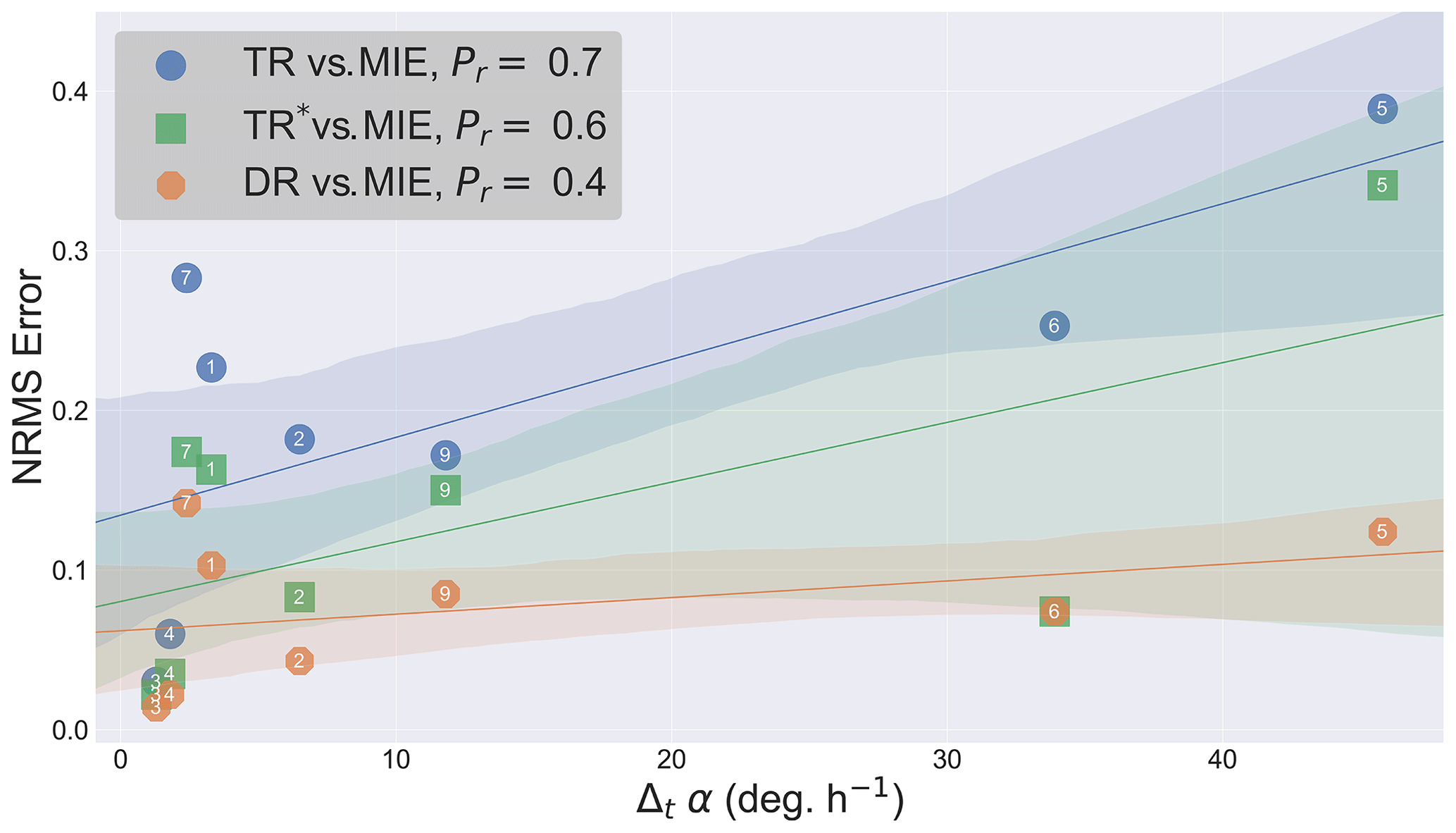
Figure 10Correlation between the NRMS error and the change in wind direction at plume height (Δtα). The shaded areas show the 90 % confidence region. Case ID is noted for each data point on the graph along with the calculated Pearson correlation coefficients (Pr) for the three methods. Results indicate a positive correlation between the NRMS error and Δtα.
4.3 Weighted upwind to downwind concentration ratio (ϕ)
In applying the mass-balance technique, the mass flux associated with upwind emissions (and regional background levels) entering the box volume (inflow) is subtracted from the downwind outgoing flux containing the emissions within the box (outflow) to estimate the net emission rate from sources within the box volume. The mass inflow associated with regional background levels (e.g., for CH4 and CO with relatively high background concentrations) is balanced out with the mass flux out of the box due to spatial (horizontal) homogeneity of background concentrations. However, emissions from upwind sources carried through the sampling region (box volume) are spatially heterogeneous (plumes) and therefore their inflow and outflow through a control volume is not necessarily equal and canceling. For instance, converging horizontal wind fields and/or plume vertical motion and mixing can result in temporary accumulation of the mass of these upwind plumes within the box (control volume). If the emissions from upwind sources are large relative to the within-box source(s), the emission rates retrieval may therefore become less accurate. That is to say, all the processes (including the ones described above in terms of ΔtRi and Δtα) that contribute to storage-release of the mass emitted by the source(s) within the flux box may also affect the mass emitted from upwind sources which are entering the box through the upwind wall(s) – leading to further increased uncertainty in the retrieved emission rates for sources within the box. The box upwind-to-downwind concentration ratio is in strong correlation with the relative magnitude of upwind emissions entering the box to the emissions from a given source within the box, with Pr≥0.8 as determined for our nine studied cases. To distinguish upwind emissions from regional background levels, this ratio can be weighted by temporal standard deviations in upwind and downwind concentrations. Hence we define
where is the screen average upwind concentration and is the plume average concentration; here the plume is defined as downwind concentrations that are one standard deviation above the mean. and are upwind and downwind concentration standard deviations. Note that while the first ratio in Eq. (19) represents the magnitude of upwind to source emissions, the second ratio distinguishes upwind plumes from background concentrations: in the absence of upwind plumes, approaches zero due to the uniform nature of background concentrations. Parameter ϕ can therefore provide a quantitative indication of the level of confidence in the retrieved emissions based on the mass-balance approach, due to this factor. Table 3 lists ϕ values in % for the nine studied cases, determined from our GEM-MACH-simulated fields.
For an isolated source with relatively low upwind emissions (which in turn depends on the mean wind direction and the location of the nearby sources) ϕ would be small and the application of the mass-balance technique would be expected to yield more accurate results. This was true for cases 3 and 4 with ϕ<0.2 % (see Fig. 2d for case 4). JOSM 2013 cases 3 and 4 were conducted over CNRL and Syncrude oil sands facilities on 20 August and 3 September 2013. For the period of these two flight cases, wind directions were also consistently from the south-west, a condition that was accurately simulated in our GEM-MACH model runs for the same period. CNRL and Syncrude are the two facilities located on the western side of the Athabasca oil sands complex, with no facilities to their west and therefore no upwind sources of emissions when wind direction is from the west (Fig. 1b). These conditions resulted in low EC,S rates of 2 % and −3 % for cases 3 and 4. For these two cases, TR estimates were within 4 %–6 % of the MIEs. Our TR estimates of SO2 emissions for CNRL were in strong agreement with TERRA SO2 emission rate estimates by Gordon et al. (2015) using aircraft-measured data during JOSM 2013 campaign, where estimates were 4.8 % higher than minute-by-minute emissions reported by CNRL. Our analysis indicates that about 3 % of this over-estimation could be due to release of the stored mass during the flight on 20 August (case 4).
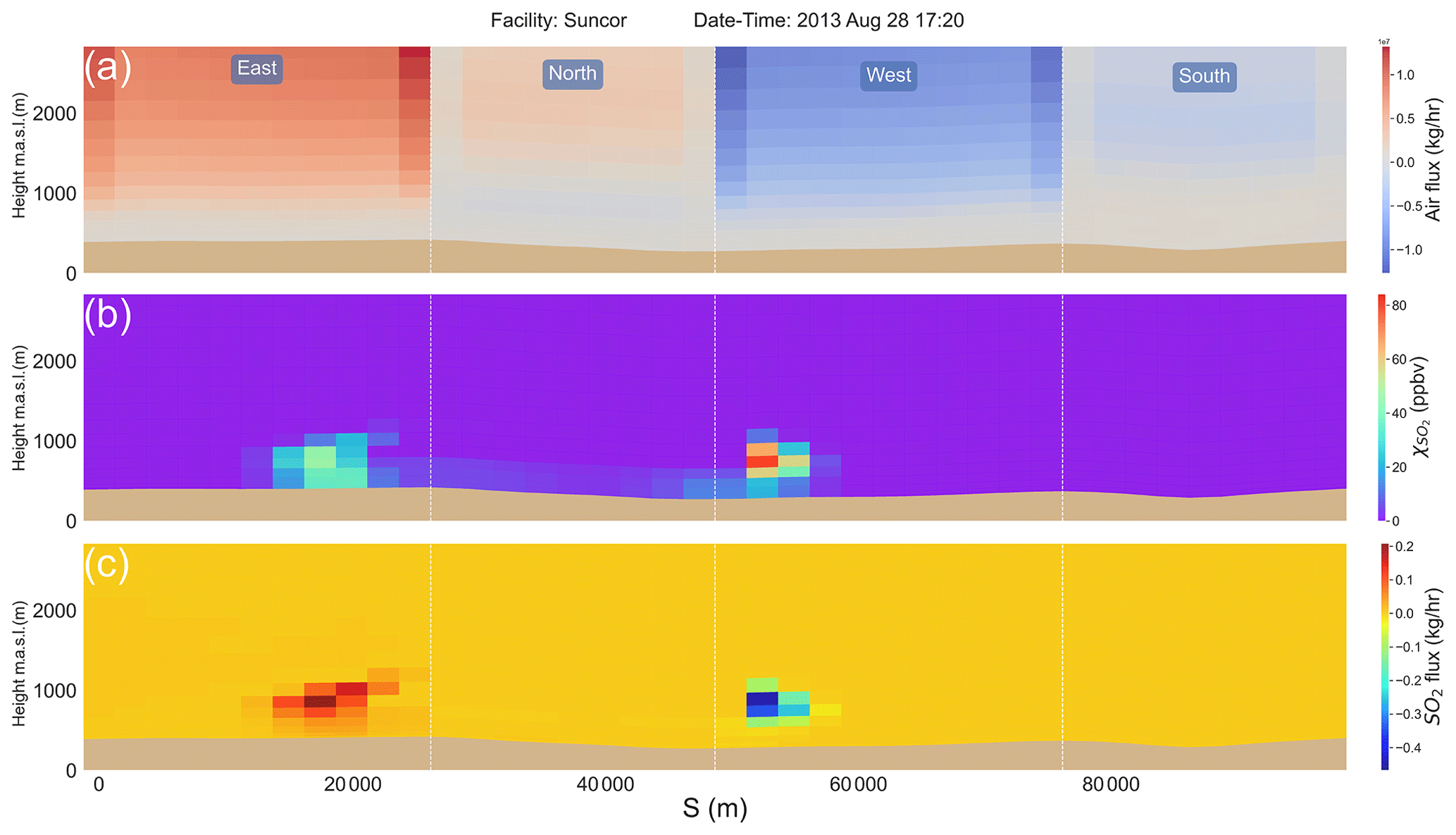
Figure 11Case 8 screens around Suncor: (a) air flux screen, (b) SO2 mixing ratio screen and (c) SO2 mass flux screen. Note the strong negative flux (inflow) on the western wall and the weaker positive flux (outflow) on the eastern wall resulting in (temporal avg.) ϕ=13 %.
Small ϕ values represent favorable conditions for applying the mass-balance technique for emission rate retrievals. For seven out of nine studied cases, ϕ was less than 10 % with NRMS errors between 4 % and 28 % for TR estimates. The opposite was true for rejected cases 5 and 8 with ϕ scores 11 % and 13 %, with NRMS errors 39 % and 166 % for TR estimates. This under performance was a combined result of upwind emissions which were higher than the source emissions, consistent converging wind fields (slower wind speeds within the flux box relative to the upwind wall throughout the flight time), and plume vertical motion due to change in atmospheric stability (ΔtRi≠0). For rejected case 5, there was an additional contribution from variations in the direction of plume transport (Δtα=46∘, sampling time average). Rejected case 8 was conducted around the Suncor facility on 28 August 2013, during which the mean wind direction was from the west; as a result, large upwind SO2 plumes originating from the Syncrude facility, located on the western side of Suncor (see Fig. 1b), continuously entered the flux box during the period of this case. SO2 mass was accumulated within the volume of the box resulting in a flight/sampling time average storage rate of 156 % of the total retrieved emission rates (see Fig. 4). Note that a large upwind source was a condition previously identified for rejecting this flight from emissions calculations (which is why emissions from this flight were not estimated in previous work). The ϕ predictor introduced here allows this effect to be quantified (from model forecasts used to plan aircraft flights, and the analysis of aircraft measured pollutant data time series). Figure 11 shows (a) air flux, (b) SO2 mixing ratio () and (c) SO2 mass flux screens around Suncor at the start of rejected case 8; note the strong negative (inwards) flux on the western wall (originating from upwind emissions from the Syncrude facility) and the weaker positive (outwards) flux on the eastern wall (Fig. 11). By accounting for the storage rate (), using model 3D data from time-consecutive screens, NRMS error was reduced by 52 % of MIEs in TR* estimates for this case. Direct retrieval (DR) of the Suncor emission rates for the period of rejected case 8, where storage was estimated directly from the model 4D data (volumetric time series), was within 23 % of MIEs. ϕ=13 % for rejected case 8 implies unsuitable conditions (>30 % uncertainty) for the application of the mass-balance technique, as the TR method failed to retrieve facility emissions (EC<0); the ϕ parameter allows a quantification of the conditions for rejection of flight data for emission rates retrieval purposes.
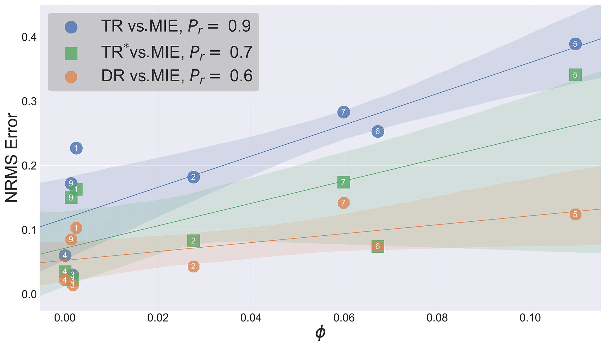
Figure 12Correlations between the NRMS error and the forecast parameter ϕ, for DR, TR and TR* estimates. The shaded areas indicate the 90 % confidence region. Case ID is indicated for each data point. Pearson correlation coefficients (Pr) for the three methods are also noted on the graph. Results indicate a strong correlation between NRMS error and the ϕ parameter.
Our results indicate a strong positive correlation between ϕ and the NRMS error (strongest among the three forecast parameters), independent of the method. Figure 12 shows this correlation for the three retrieval methods, note that rejected case 8 was excluded from correlation analysis as an outlier (extreme storage event) since its inclusion would dominate the correlation and obscure the information from the other data points. Pearson correlation coefficients (Pr) for DR, TR and TR* were calculated as 0.6, 0.9 and 0.7, respectively. That is, a significant proportion of the variability in the emissions retrieval NRMS error can be accounted for by each of the metrics proposed here. In aircraft-based retrievals, analysis of ϕ can provide insights into the expected reliability of the retrieved emissions and the probability of storage-release events. Pre-flight model forecasts of ϕ can be used for the same purpose. For ϕ scores greater than 10 %, the uncertainty in the retrieved emission rates due to storage release is over 30 %. For such conditions, it is advised that the storage rate (EC,S) be estimated from time-consecutive screens and/or vertical profiles of relevant fields. This can be achieved by conducting multiple box flights and/or downwind vertical profiling over the sampling time in order to estimate for improved top-down emission rate retrievals (TR*; see Sects. 2.2.3 and 3.3).
4.4 Summary of predictive methods
The three forecast parameters ΔtRi, Δtα and ϕ as discussed above provide a new approach for analyzing the uncertainty levels associated with potential storage-release events during aircraft-based emission rate retrieval flight time, either using a priori meteorological forecasts to provide guidance for emissions retrieval flight decision making or in post-processing of already completed flights. Table 2 summarizes the correlations between these parameters and the NRMS error in estimates by the TR method in terms of Pr correlation coefficients and the slopes (m) of the best fit lines (least squares) in Figs. 8, 10 and 12. The last row in Table 2, demonstrates the correlation between the changes in the two meteorological forecast parameters ΔtRi and Δtα and change in NRMS error levels; accordingly, net changes of 0.57 h−1 in and 60∘ h−1 in Δtα during the flight/sampling time may result in 30 % (or more when both contribute) uncertainty in the estimates, the maximum estimated uncertainty (30 %) for TERRA SO2 emission rate retrievals in Gordon et al. (2015). The combined effects of h−1 and Δtα=46∘ h−1 during the ∼2 h flight time of case 5, contributed to a net error of 39 % in TR estimates for this case. Further, for any forecasted/estimated rate of change in meteorology in terms of ΔtRi and Δtα, shorter sampling intervals (e.g., two flights in tandem, vertical profiling information) may result in more confidence in the estimated emission rates; small values of ΔtRi and Δtα correspond to steady-state conditions, whereas higher values correspond to increased uncertainty in the estimates due to storage-release events. The NRMS errors in TR estimates for cases with ϕ<10 % (seven out of nine) were less than 30 %. ϕ>10 % correspond to over 30 % uncertainty in the estimates, as for rejected cases 5 and 8. Note that cases 5 and 8 were excluded (rejected) from TERRA retrievals in previous work due to unfavorable conditions for the application of TERRA. Here, using GEM-MACH-predicted fields, we were able to quantify the impact of changing meteorology and/or high upwind emissions in mass-balance emission rate retrieval for these two cases in terms of the three forecast parameters ΔtRi, Δtα and ϕ as described above.
Table 2Summary of correlations between NRMS error in TR estimates and the three forecast parameters for storage-release events, in terms of the Pearson correlation coefficient (Pr), and fit line (least squares) slopes (m) in Figs. 8, 10 and 12. The last row indicates the amount of change in forecast parameters that would result in >=30 % error in estimates. ϕ<10 % corresponds to <30 % error.
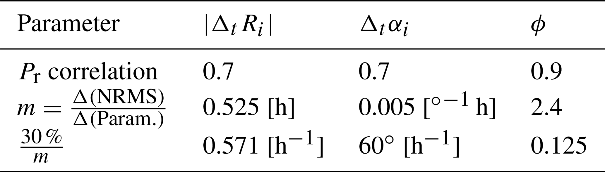
We have examined storage and release events in the specific context of “box” flights around an emitting facility, however note that other strategies have been put forward in the literature (e.g., near-field downwind transects, Peischl et al., 2010). We note: (1) the heterogeneous nature of meteorology even at the scales employed for the box flights here suggests that the impact of storage and release will likely be greater as the distance between screen(s) and emission source(s) increases (for example, see Appendix C, Fig. C1, for case 8, where the contribution of the storage term increases as a function of downwind distance): short distance “box” flights such as examined here would reduce the storage and release impact; (2) our ΔtRi and Δtα parameters may nevertheless be applied to “single-leg” downwind transects retrievals, and repeat flights (e.g., by a second aircraft following behind the first aircraft) may be one way of reducing storage and release uncertainties in these flights; (3) our ϕ parameter relies on the availability of upwind information and hence is not applicable for “single-leg” (e.g., downwind transects) retrievals. (4) Our ϕ parameter provided the strongest correlation between storage and release and retrieval outcomes and therefore, where possible, should be estimated from additional upwind observations. These findings suggest that, while some aspects of storage and release can be identified with “single-leg” downwind flights, the impacts of storage and release for these flight patterns may be higher than for “box” flight patterns such as studied here.
Table 3 provides a summary of all the meteorological conditions and emission scenarios in our GEM-MACH model simulations for the period of the nine studied JOSM 2013 cases. The three forecast parameters are also provided in the table: the average rate of change in atmospheric stability represented by ΔtRi, the average rate of change in wind direction at plume height (change in direction of the transport) represented by Δtα and the weighted upwind-to-downwind concentration ratio parameter (ϕ). Estimates by the three described methods (DR, TR and TR*) are compared to MIEs, and the corresponding normalized (to MIE) mean (NM) and root-mean-square (NRMS) errors are listed for each of the studied cases.
Table 3A summary of the meteorological conditions and source emission scenarios by the three oil sands facilities for the period of the nine JOSM 2013 box flight cases in our GEM-MACH model simulations. Flight date-time and duration is provided for each case, LT stands for local time (UT−6 h). The flight time average , wind speed and direction at plume height are shown. The three forecast parameters are also provided: ΔtRi, Δtα and ϕ. DR, TR and TR* method estimates are compared to model input emissions (MIEs). Storage (S) and/or release (R) events, their order of occurrence (for the cases where both were present) and their relative magnitude (the bigger contribution is represented by boldface letters) are given. The flight time average storage rate as a fraction (%) of the total retrieved emission rates are also provided for each case. The performance of the three retrieval methods against MIE, are shown in terms of NM and NRMS errors.
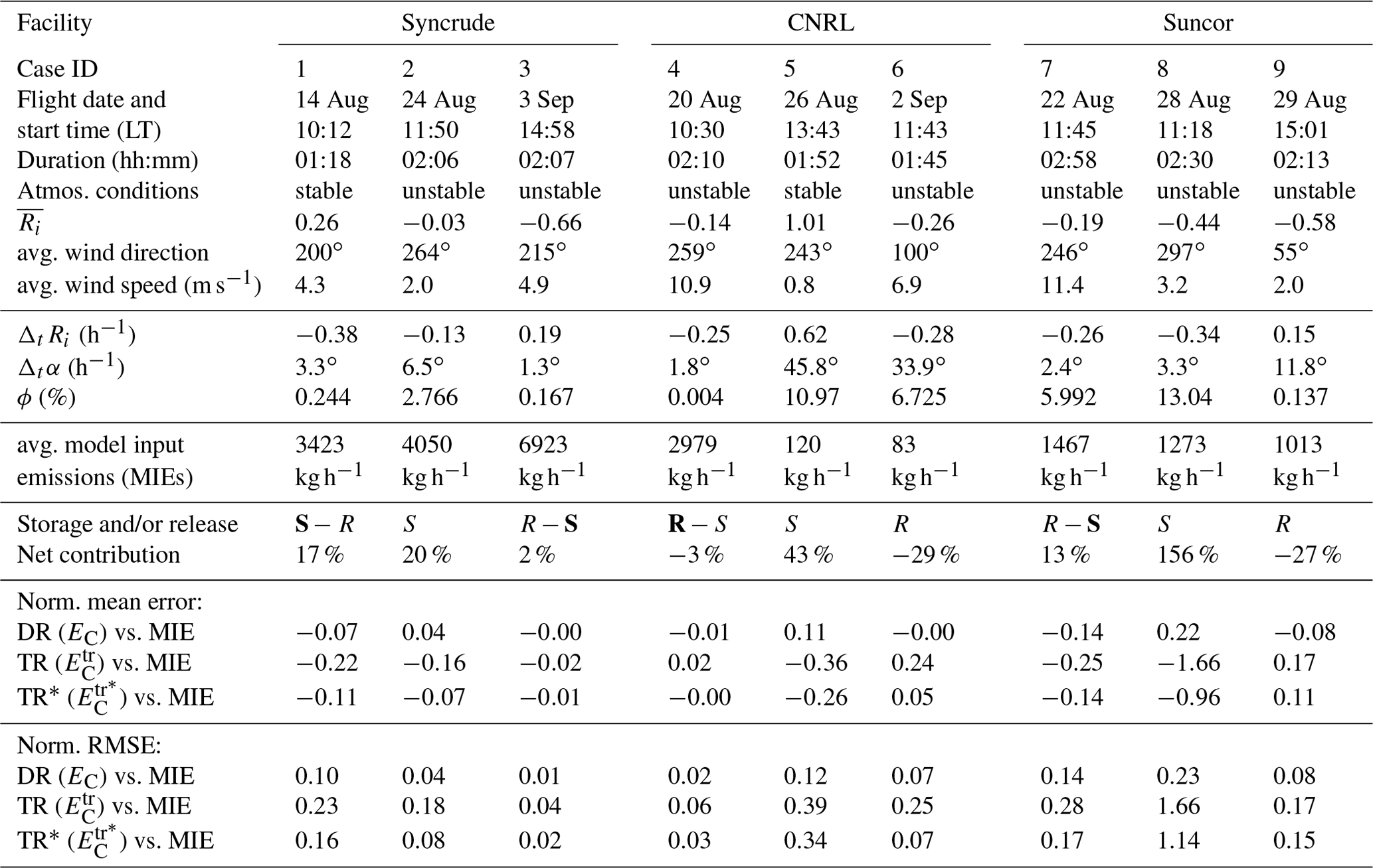
We have carried out a series of retrospective air-quality simulations employing Environment and Climate Change Canada's (ECCC) air-quality model, Global Environmental Multiscale – Modelling Air-quality and Chemistry (GEM-MACH), for the period of the JOSM 2013 campaign over the Athabasca oil sands region, with the primary objective of evaluating aircraft-based mass balance emission rate retrievals such as applied in TERRA (i.e., the Top-down Emission Rate Retrieval Algorithm). We considered the simulations of nine JOSM 2013 emission estimation flight cases, over three oil sands facilities with high SO2 emissions (CNRL, Syncrude and Suncor), and used GEM-MACH model 4D output data as a surrogate for aircraft measurements in emission rate estimations to evaluate the application of the mass-balance approach in top-down methodologies. Although the emphasis was on SO2 emissions, the explored concepts and the three forecast parameters developed here are also applicable to species with high background levels (e.g., CH4, CO). Emissions retrievals were made by analyzing GEM-MACH model output data through three different approaches: (a) direct retrieval (DR) of the model input emissions (MIEs) by analyzing GEM-MACH model 4D data (volumetric time series) through a comprehensive analysis of all of the processes contributing to the change in mass within the control volume (flux box) including vertical and horizontal fluxes through box top and lateral walls, surface deposition and rate of storage of mass within the volume of the box, (b) TERRA retrieval (TR) approximations by limiting our analysis to the model data on 2D screens comprised of lateral walls of the flux box surrounding the emission source, mimicking aircraft-based retrievals during an emission estimation (box) flight, and (c) improved TERRA retrievals (TR*) through estimation of the rate of change in the stored mass within the volume of the flux box by analyzing the data on time-consecutive 2D screens at each model time step (3D). See Table 1 for a summary of the three methods.
Results were compared to the MIEs and the performance of the three methods was analyzed in terms of normalized (to MIE) root-mean-square (NRMS) error. The DR method estimates (EC) were within 1 %–23 % of MIE for all nine studied cases. TR and TR* ( and ) estimates for seven out of nine cases were within 4 %–28 % and 2 %–17 % of MIEs, respectively. This range of emissions retrieval error was similar to the range (±30 %) estimated from aircraft observations in previous work (Gordon et al., 2015), with the remaining 2 flights (rejected cases 5 and 8) excluded in previous work due to unsuitable meteorological conditions and knowledge of upwind emissions. Estimates for the JOSM case on 26 August 2013 around the CNRL facility (rejected case 5) were impacted by change in atmospheric stability at rate h−1 and shift in wind direction at plume center-point (maximum concentration) height at rate Δtα=46∘ h−1 during the ∼2 h flight time; NRMS errors for this case in estimates by the TR and TR* methods were 39 % and 34 %, respectively. Estimates for the case on 28 August around the Suncor facility (rejected case 8) were impacted by high emissions (relative to source emission rates) from the upwind oil sands facility Syncrude (avg. ϕ=13 %) and change in atmospheric stability at rate h−1 during the ∼2.5 h flight/sampling time; NRMS errors for this case were 166 % and 114 % by the TR and TR* methods, respectively. The under-performance in rejected cases 5 and 8 estimates were the consequence of several different factors and conditions during the flight time; we refer to the collective impact of these conditions as storage-and-release events. The nine studied cases were affected by storage-release events at various degrees, ranging from −29 % to 156 % with a median of 13 %. This range for the seven cases that are included in past work with TERRA applications is −29 % to 20 % with a 2 % median.
Storage-release events occur when temporal and spatial variations in meteorological conditions and/or source emission rate result in a temporary imbalance between the addition of mass to the volume of the box through source emissions and removal of mass by vertical and horizontal fluxes through box top and lateral walls and the deposition to ground surface. The transient storage of the emitted mass within box volume and its later release contribute to emission rate over- and under-estimations based on the mass-balance technique. We introduced a correction term, EC,S, in the mass-balance equation to represent the rate of storage release. Utilizing GEM-MACH model output data, we investigated the contribution of this term to the total integrated retrieved emission rates. The storage rate term (EC,S) contributed over 20 % of the total retrieved emissions for five out of nine cases, signifying the impact of storage-release events in emission rate retrievals based on the mass-balance approach. The corresponding uncertainties in estimated emission rates were quantified for each of the nine studied cases, and conditions giving rise to storage-release events were extensively explored.
We have introduced an approach for estimating the storage term as the TR* method, based on estimations of the rate of change in the stored mass within the box volume from data on time-consecutive 2D screens and/or vertical profiles around and downwind of the same emission source (3D dataset). We have shown that by estimating the storage term () in this way, estimates can be improved by 2 %–52 % of MIE. Three forecast parameters were introduced for predicting/identifying the probability of storage-release events: variations in atmospheric dynamic stability represented by change in gradient Richardson number (ΔtRi), shift in the direction of transport represented by variations in wind direction at plume height (Δtα), and the weighted upwind to downwind concentration ratio (ϕ). We have demonstrated the strong correlation between these three parameters and the NRMS error in mass-balance estimates and discussed the potential of utilizing the three forecast parameters in analysis of the uncertainty levels in aircraft-based top-down emission rate retrieval methodologies. Model-based forecasts of these parameters can also provide practical advice for the planning of future airborne measurement campaigns.
The investigation carried out here has resulted in the creation of quantitative measures for the extent to which storage and release events may impact aircraft emissions retrieval accuracy. Retrieval uncertainties, using regional air-quality model output, were shown to be of similar magnitude to previously published values, with the exception of cases where the underlying assumption of time-invariant meteorological conditions was not valid and/or where significant upwind emissions impacted the estimates. We have also devised a methodology to reduce the impact of this form of emissions retrieval error by estimating the storage rate () through (a) the use of repeat flights, around the same facility, either with a single or multiple aircraft(s), or (b) aircraft-based remote vertical profiling (e.g., lidar measurements) of relevant fields during the sampling period.
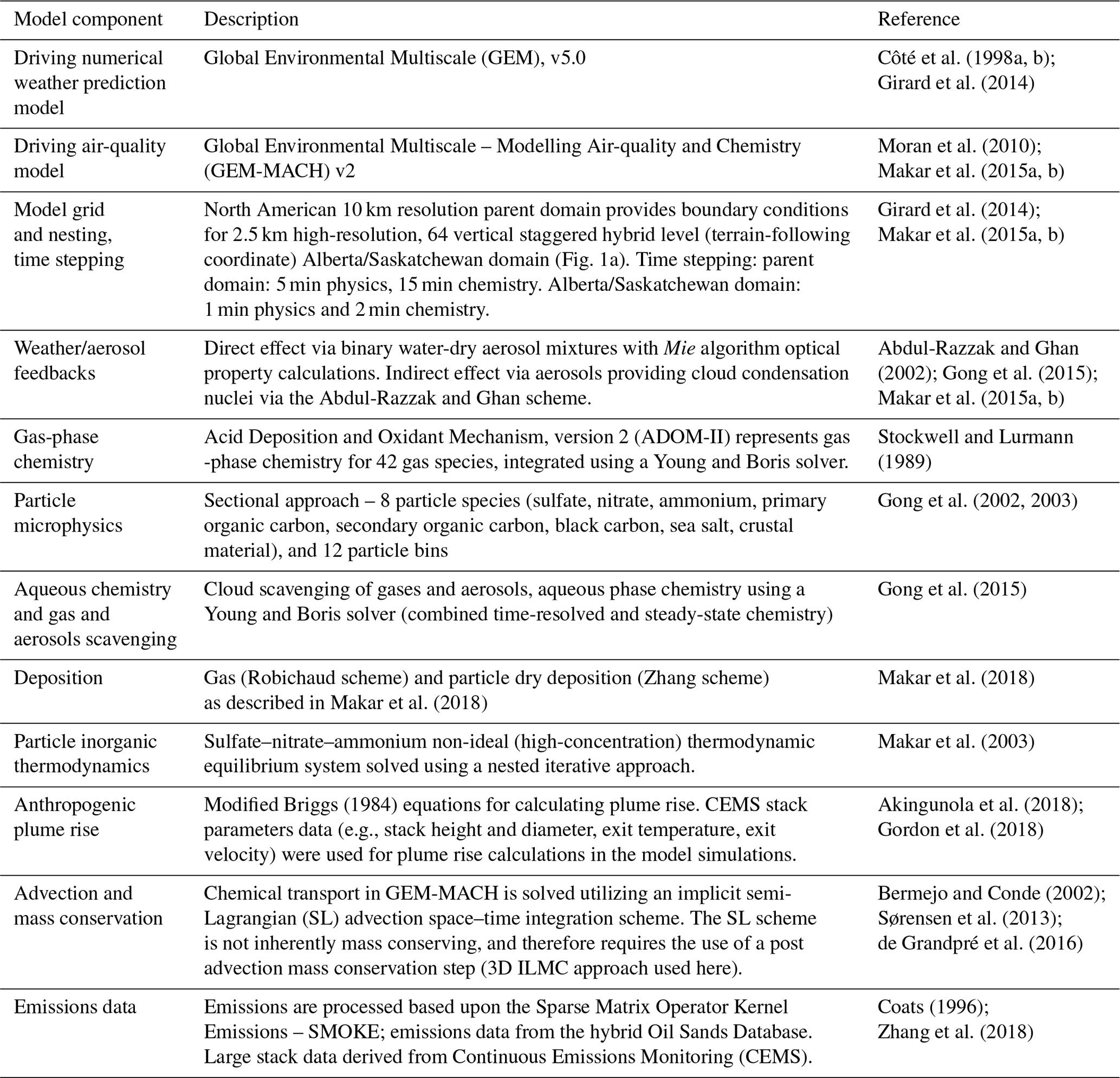
B1 Derivations for mass-balance terms
The net horizontal flux exiting through lateral walls of the box (EC,H) is calculated by extracting compound mixing ratio (χC), air density (ρair) and the wind normal to the lateral walls of the box from the model output, and integrating over the surface (2D screen) comprised of box lateral walls at each time step,
where s(x,y) is the screen path coordinate, which follows the horizontal projection of the box flight path around the facility in a counter-clockwise direction.
The normal wind (positive outwards) along the screen is calculated as
where U and V are wind components towards east (x) and north (y), respectively.
The vertical flux through the box top can be calculated as
where and are compound mixing ratio and the vertical wind component (positive upwards) at the box top. In the observational application of the retrieval methodology, the top of the box corresponds to an aircraft measurement altitude which is above the plume.
The horizontal air flux through the screen (positive outwards) is calculated from extracted air density and wind fields along the screen at time t as
The rate of change in the air mass (accumulation) within the box due to changing air density (compressible fluid) can be estimated as
The vertical air flux leaving the box (positive upwards) is calculated similar to Eq. (B3),
Table B1Discrete integral expressions of Eqs. (4), (5), (B1) and (B3) to be substituted in Eq. (7). Constants Δx, Δy and Δs are equal to model grid resolution in the horizontal, 2.5 km. t is the time index; i, j and k are the 3D-space indices and s is the path index around the box.
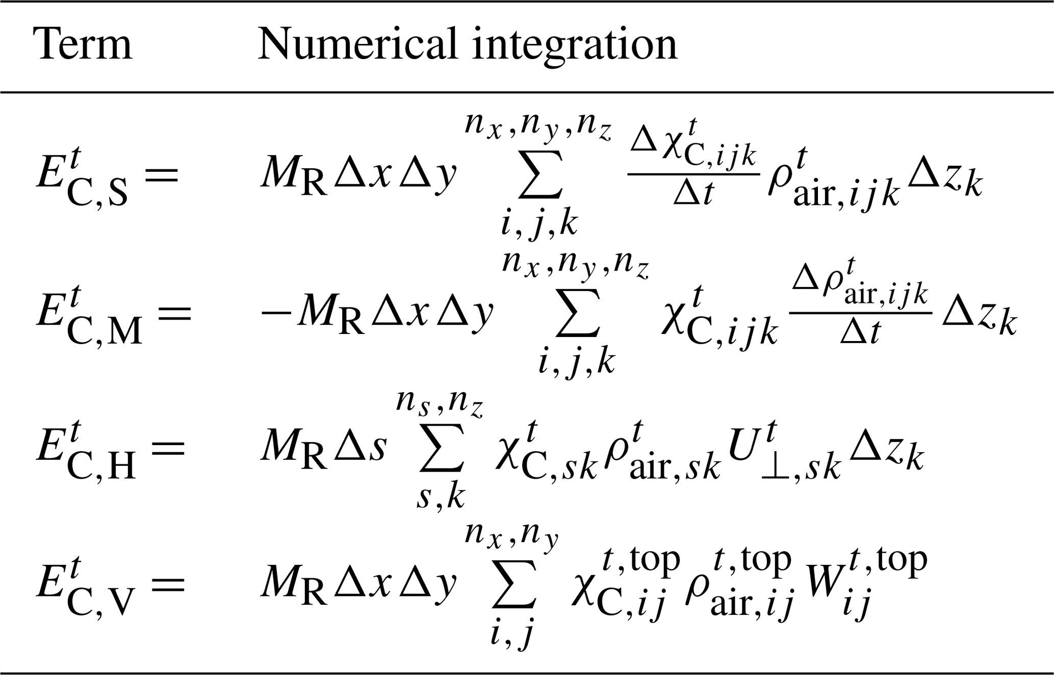
Table B2Discrete integral expressions for Eqs. (B4) and (8)–(10) to be substituted in Eq. (12) for TR method estimations. Terms and variables are listed in the order needed for calculating the dependent terms. Δs is constant and equal to model horizontal grid resolution, 2.5 km. t and s are time and path indices, respectively. A is the box base area. Point (io, jo) is at the box horizontal center.
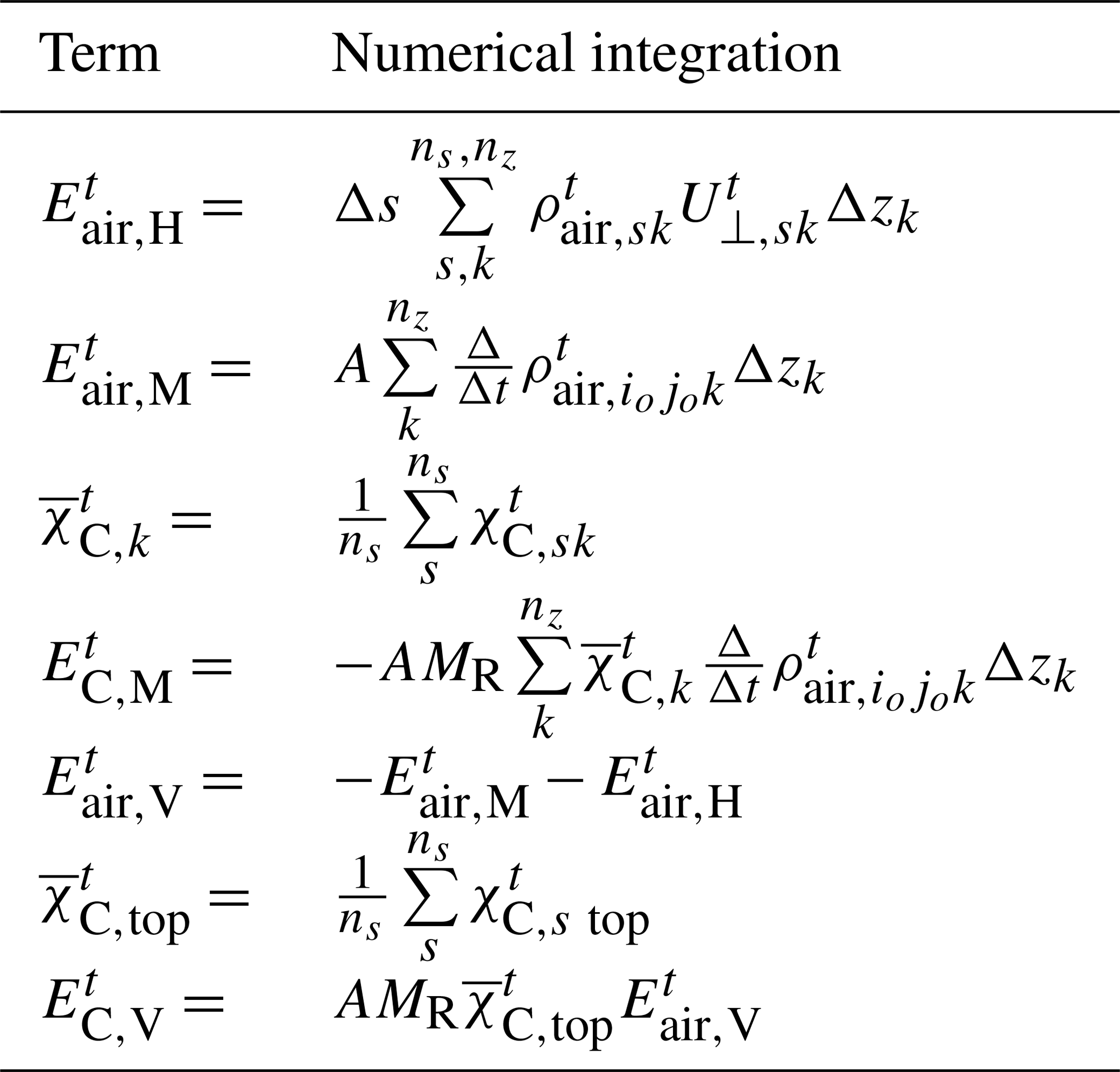
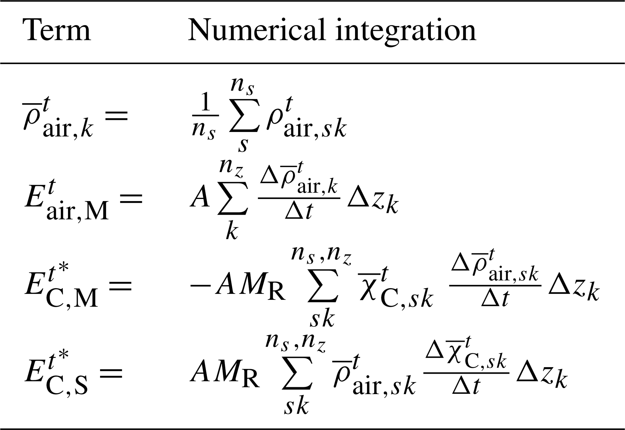
B2 Discrete integral expressions (Tables B1–B3)
The numerical integration expressions for calculating the terms in Eqs. (7), (12) and (16), using model data, are described in Tables B1–B3. Throughout, the second-order central finite-difference scheme (Jacobson, 2005) was used to numerically solve the time derivatives () with the residual error of order O(Δt2), where Δt is equal to the 2 min ( h) model time step. Surface deposition rates () were extracted directly from the model output for the area covered by the base of the flux box for each case, to eliminate deposition estimates as a potential source of error in retrievals. Note that in Table B2, the species vertical mass flux () is calculated using the estimated vertical air mass flux () from the mass-balance equation for air (Eq. 8) and the box top average mixing ratio ().
Figure C1The contribution of the storage rate term (EC,S) to the net retrieved emission rates (EC) as a function of downwind distance for case 8. As shown in the wind-rose diagram, the wind direction for this case was towards south–east (S–E), and therefore the downwind dependence is shown in two directions west–east (green squares) and north–south (red circles). The contribution of storage increases as a function of downwind distance. This suggests that the impact of storage release may increase as the distance between the downwind screen (sampling location) and the emission sources increase. A similar dependence of the magnitude of the storage release with downwind distance was observed for the other cases.
Note that this work made use of an air-quality model: no observational datasets were used in this work. The model results are available upon request to Paul Makar (paul.makar@ec.gc.ca). GEM-MACH, the atmospheric chemistry library for the GEM numerical atmospheric model (©2007–2013, Air Quality Research Division and National Prediction Operations Division, Environment and Climate Change Canada), is a free software which can be redistributed and/or modified under the terms of the GNU Lesser General Public License as published by the Free Software Foundation – either version 2.1 of the license or any later version. The specific GEM-MACH version used in this work may be obtained on request to paul.makar@ec.gc.ca. Much of the emissions data used in our model are available online: Executive Summary, Joint Oil Sands Monitoring Program Emissions Inventory report (https://www.canada.ca/en/environment-climate-change/services/science-technology/publications/joint-oil-sands-monitoring-emissions-report.html; JOSM, 2016); and Joint Oil Sands Emissions Inventory Database (http://ec.gc.ca/data_donnees/SSB-OSM_Air/Air/Emissions_inventory_files/; JOSM, 2018). More recent updates may be obtained by contacting Junhua Zhang (junhua.zhang@ec.gc.ca).
SF wrote the paper with supervision and input from MG and PAM. SF ran the GEM-MACH simulations and implemented the mass-balance retrieval algorithm into GEM-MACH. PAM coordinated the GEM-MACH work. AA setup the GEM-MACH code and provided simulation support. AD, JL, KH, and SML provided advice during analysis and contributed to paper revisions.
Some of the authors are members of the editorial board of Atmospheric Chemistry and Physics. The peer-review process was guided by an independent editor, and the authors also have no other competing interests to declare.
Publisher's note: Copernicus Publications remains neutral with regard to jurisdictional claims in published maps and institutional affiliations.
This work was funded under the Oil Sands Monitoring (OSM) Program. It is independent of any position of the OSM Program.
This research has been supported by the Oil Sands Monitoring Program (grant no. A-PD-6; Integrated Atmospheric Deposition Monitoring), and the Natural Sciences and Engineering Research Council of Canada – NSERC (grant no. RGPIN 2015-04292).
This paper was edited by Joshua Fu and reviewed by Wayne Angevine and two anonymous referees.
Abdul-Razzak, H. and Ghan, S. J.: A parameterization of aerosol activation 3. Sectional representation, J. Geophys. Res.-Atmos., 107, AAC 1-1–AAC 1-6, https://doi.org/10.1029/2001JD000483, 2002. a
Aggarwal, M., Whiteway, J., Seabrook, J., Gray, L., Strawbridge, K., Liu, P., O'Brien, J., Li, S.-M., and McLaren, R.: Airborne lidar measurements of aerosol and ozone above the Canadian oil sands region, Atmos. Meas. Tech., 11, 3829–3849, https://doi.org/10.5194/amt-11-3829-2018, 2018. a
Akingunola, A., Makar, P. A., Zhang, J., Darlington, A., Li, S.-M., Gordon, M., Moran, M. D., and Zheng, Q.: A chemical transport model study of plume-rise and particle size distribution for the Athabasca oil sands, Atmos. Chem. Phys., 18, 8667–8688, https://doi.org/10.5194/acp-18-8667-2018, 2018. a, b, c
AMS – American Meteorological Society: Gradient Richardson number, Glossary of Meteorology, available at: http://glossary.ametsoc.org/wiki/Gradient_richardson_number (last access: 5 September 2021), 2021a. a
AMS – American Meteorological Society: Ekman spiral, Glossary of Meteorology, available at: https://glossary.ametsoc.org/wiki/Ekman_spiral (last access: 5 September 2021), 2021b. a
Angevine, W. M., Peischl, J., Crawford, A., Loughner, C. P., Pollack, I. B., and Thompson, C. R.: Errors in top-down estimates of emissions using a known source, Atmos. Chem. Phys., 20, 11855–11868, https://doi.org/10.5194/acp-20-11855-2020, 2020. a, b
Baray, S., Darlington, A., Gordon, M., Hayden, K. L., Leithead, A., Li, S.-M., Liu, P. S. K., Mittermeier, R. L., Moussa, S. G., O'Brien, J., Staebler, R., Wolde, M., Worthy, D., and McLaren, R.: Quantification of methane sources in the Athabasca Oil Sands Region of Alberta by aircraft mass balance, Atmos. Chem. Phys., 18, 7361–7378, https://doi.org/10.5194/acp-18-7361-2018, 2018. a
Barchyn, T. E., Hugenholtz, C. H., Myshak, S., and Bauer, J.: A UAV-based system for detecting natural gas leaks, J. Unman. Vehic. Syst., 6, 18–30, https://doi.org/10.1139/juvs-2017-0018, 2018. a
Bélair, S., Brown, R., Mailhot, J., Bilodeau, B., and Crevier, L.-P.: Operational Implementation of the ISBA Land Surface Scheme in the Canadian Regional Weather Forecast Model. Part II: Cold Season Results, J. Hydrometeorol., 4, 371–386, https://doi.org/10.1175/1525-7541(2003)4<371:OIOTIL>2.0.CO;2, 2003a. a
Bélair, S., Crevier, L.-P., Mailhot, J., Bilodeau, B., and Delage, Y.: Operational Implementation of the ISBA Land Surface Scheme in the Canadian Regional Weather Forecast Model. Part I: Warm Season Results, J. Hydrometeorol., 4, 352–370, https://doi.org/10.1175/1525-7541(2003)4<352:OIOTIL>2.0.CO;2, 2003b. a
Bermejo, R. and Conde, J.: A Conservative Quasi-Monotone Semi-Lagrangian Scheme, Mon. Weather Rev., 130, 423–430, https://doi.org/10.1175/1520-0493(2002)130<0423:ACQMSL>2.0.CO;2, 2002. a
Briggs, G. A.: Plume rise and buoyancy effects, atmospheric sciences and power production, in: DOE/TIC-27601 (DE84005177), edited by: Randerson, D., TN, Technical Information Center, US Dept. of Energy, Oak Ridge, USA, 327–366, 1984. a
Cambaliza, M. O. L., Shepson, P. B., Caulton, D. R., Stirm, B., Samarov, D., Gurney, K. R., Turnbull, J., Davis, K. J., Possolo, A., Karion, A., Sweeney, C., Moser, B., Hendricks, A., Lauvaux, T., Mays, K., Whetstone, J., Huang, J., Razlivanov, I., Miles, N. L., and Richardson, S. J.: Assessment of uncertainties of an aircraft-based mass balance approach for quantifying urban greenhouse gas emissions, Atmos. Chem. Phys., 14, 9029–9050, https://doi.org/10.5194/acp-14-9029-2014, 2014. a, b
Cheng, Y., Li, S.-M., Liggio, J., Gordon, M., Darlington, A., Zheng, Q., Moran, M., Liu, P., and Wolde, M.: Top-Down Determination of Black Carbon Emissions from Oil Sand Facilities in Alberta, Canada Using Aircraft Measurements, Environ. Sci. Technol., 54, 412–418, https://doi.org/10.1021/acs.est.9b05522, 2020. a
Coats, C. J.: High-performance algorithms in the sparse matrix operator kernel emissions (SMOKE) modeling system, in: Proceedings of the Ninth AMS Joint Conference on Applications of Air Pollution Meteorology with AWMA, 28 January–2 February 1996, American Meteorological Society, Atlanta, GA, USA, 584–588, 1996. a
Conley, S., Faloona, I., Mehrotra, S., Suard, M., Lenschow, D. H., Sweeney, C., Herndon, S., Schwietzke, S., Pétron, G., Pifer, J., Kort, E. A., and Schnell, R.: Application of Gauss's theorem to quantify localized surface emissions from airborne measurements of wind and trace gases, Atmos. Meas. Tech., 10, 3345–3358, https://doi.org/10.5194/amt-10-3345-2017, 2017. a, b, c, d
Côté, J., Desmarais, J.-G., Gravel, S., Méthot, A., Patoine, A., Roch, M., and Staniforth, A.: The Operational CMC–MRB Global Environmental Multiscale (GEM) Model. Part II: Results, Mon. Weather Rev., 126, 1397–1418, https://doi.org/10.1175/1520-0493(1998)126<1397:TOCMGE>2.0.CO;2, 1998a. a, b
Côté, J., Gravel, S., Méthot, A., Patoine, A., Roch, M., and Staniforth, A.: The Operational CMC–MRB Global Environmental Multiscale (GEM) Model. Part I: Design Considerations and Formulation, Mon. Weather Rev., 126, 1373–1395, https://doi.org/10.1175/1520-0493(1998)126<1373:TOCMGE>2.0.CO;2, 1998b. a, b, c
de Grandpré, J., Tanguay, M., Qaddouri, A., Zerroukat, M., and McLinden, C. A.: Semi-Lagrangian Advection of Stratospheric Ozone on a Yin–Yang Grid System, Mon. Weather Rev., 144, 1035–1050, https://doi.org/10.1175/MWR-D-15-0142.1, 2016. a, b
Elston, J., Argrow, B., Stachura, M., Weibel, D., Lawrence, D., and Pope, D.: Overview of Small Fixed-Wing Unmanned Aircraft for Meteorological Sampling, J. Atmos. Ocean. Tech., 32, 97–115, https://doi.org/10.1175/JTECH-D-13-00236.1, 2015. a
Fathi, S.: Evaluating the Top-down Emission Rate Retrieval Algorithm (TERRA) Using Virtual Aircraft-based Sampling Within the GEM-MACH Model, MS thesis, York University, York, available at: http://hdl.handle.net/10315/34547 (last access: 5 September 2021), 2017. a
Fillion, L., Tanguay, M., Lapalme, E., Denis, B., Desgagne, M., Lee, V., Ek, N., Liu, Z., Lajoie, M., Caron, J.-F., and Pagé, C.: The Canadian Regional Data Assimilation and Forecasting System, Weather Forecast., 25, 1645–1669, https://doi.org/10.1175/2010WAF2222401.1, 2010. a
Girard, C., Plante, A., Desgagné, M., McTaggart-Cowan, R., Côté, J., Charron, M., Gravel, S., Lee, V., Patoine, A., Qaddouri, A., Roch, M., Spacek, L., Tanguay, M., Vaillancourt, P. A., and Zadra, A.: Staggered Vertical Discretization of the Canadian Environmental Multiscale (GEM) Model Using a Coordinate of the Log-Hydrostatic-Pressure Type, Mon. Weather Rev., 142, 1183–1196, https://doi.org/10.1175/MWR-D-13-00255.1, 2014. a, b, c, d
Gong, S. L., Barrie, L. A., and Lazare, M.: Canadian Aerosol Module (CAM): A size-segregated simulation of atmospheric aerosol processes for climate and air quality models 2. Global sea-salt aerosol and its budgets, J. Geophys. Res.-Atmos., 107, AAC 13-1–AAC 13-14, https://doi.org/10.1029/2001JD002004, 2002. a
Gong, S. L., Barrie, L. A., Blanchet, J.-P., von Salzen, K., Lohmann, U., Lesins, G., Spacek, L., Zhang, L. M., Girard, E., Lin, H., Leaitch, R., Leighton, H., Chylek, P., and Huang, P.: Canadian Aerosol Module: A size-segregated simulation of atmospheric aerosol processes for climate and air quality models 1. Module development, J. Geophys. Res.- Atmos., 108, AAC 3-1–AAC 3-16, https://doi.org/10.1029/2001JD002002, 2003. a
Gong, W., Makar, P., Zhang, J., Milbrandt, J., Gravel, S., Hayden, K., Macdonald, A., and Leaitch, W.: Modelling aerosol–cloud–meteorology interaction: A case study with a fully coupled air quality model (GEM-MACH), Atmos. Environ., 115, 695–715, https://doi.org/10.1016/j.atmosenv.2015.05.062, 2015. a, b
Gordon, M., Li, S.-M., Staebler, R., Darlington, A., Hayden, K., O'Brien, J., and Wolde, M.: Determining air pollutant emission rates based on mass balance using airborne measurement data over the Alberta oil sands operations, Atmos. Meas. Tech., 8, 3745–3765, https://doi.org/10.5194/amt-8-3745-2015, 2015. a, b, c, d, e, f, g, h, i, j, k, l, m, n, o, p, q, r
Gordon, M., Makar, P. A., Staebler, R. M., Zhang, J., Akingunola, A., Gong, W., and Li, S.-M.: A comparison of plume rise algorithms to stack plume measurements in the Athabasca oil sands, Atmos. Chem. Phys., 18, 14695–14714, https://doi.org/10.5194/acp-18-14695-2018, 2018. a
Jacobson, M. Z.: Fundamentals of Atmospheric Modeling, 2nd Edn., Cambridge University Press, Cambridge,https://doi.org/10.1017/CBO9781139165389, 2005. a
JOSM: Joint Oil Sands Monitoring Plan, Integrated Monitoring Plan for the Oil Sands, Air Quality Component, p. 72, available at: http://publications.gc.ca/site/eng/394253/publication.html (last access: 5 September 2021), 2011. a, b
JOSM: Environment and Climate Change Canada and Alberta Environment and Parks, Executive Summary, Joint Oil Sands Monitoring Program Emissions Inventory report, JOSM [data set], available at: https://www.canada.ca/en/environment-climate-change/services/science-technology/publications/joint-oil-sands-monitoring-emissions-report.html (last access: 5 September 2021), 2016. a
JOSM: Environment and Climate Change Canada and Alberta Environment and Parks, Joint Oil Sands Emissions Inventory Database, JOSM [data set], available at: http://ec.gc.ca/data_donnees/SSB-OSM_Air/Air/Emissions_inventory_files/, (last access: 5 September 2021), 2018. a
Kalthoff, N., Corsmeier, U., Schmidt, K., Kottmeier, C., Fiedler, F., Habram, M., and Slemr, F.: Emissions of the city of Augsburg determined using the mass balance method, Atmosp. Environ., 36, 19–31, https://doi.org/10.1016/S1352-2310(02)00215-7, 2002. a, b, c
Karion, A., Sweeney, C., Pétron, G., Frost, G., Michael Hardesty, R., Kofler, J., Miller, B. R., Newberger, T., Wolter, S., Banta, R., Brewer, A., Dlugokencky, E., Lang, P., Montzka, S. A., Schnell, R., Tans, P., Trainer, M., Zamora, R., and Conley, S.: Methane emissions estimate from airborne measurements over a western United States natural gas field, Geophys. Res. Lett., 40, 4393–4397, https://doi.org/10.1002/grl.50811, 2013. a
Karion, A., Sweeney, C., Kort, E. A., Shepson, P. B., Brewer, A., Cambaliza, M., Conley, S. A., Davis, K., Deng, A., Hardesty, M., Herndon, S. C., Lauvaux, T., Lavoie, T., Lyon, D., Newberger, T., Pétron, G., Rella, C., Smith, M., Wolter, S., Yacovitch, T. I., and Tans, P.: Aircraft-Based Estimate of Total Methane Emissions from the Barnett Shale Region, Environ. Sci. Technol., 49, 8124–8131, https://doi.org/10.1021/acs.est.5b00217, 2015. a
Karion, A., Lauvaux, T., Lopez Coto, I., Sweeney, C., Mueller, K., Gourdji, S., Angevine, W., Barkley, Z., Deng, A., Andrews, A., Stein, A., and Whetstone, J.: Intercomparison of atmospheric trace gas dispersion models: Barnett Shale case study, Atmos. Chem. Phys., 19, 2561–2576, https://doi.org/10.5194/acp-19-2561-2019, 2019. a
Li, J. and Barker, H. W.: A Radiation Algorithm with Correlated-k Distribution. Part I: Local Thermal Equilibrium, J. Atmos. Sci., 62, 286–309, https://doi.org/10.1175/JAS-3396.1, 2005. a
Li, S.-M., Leithead, A., Moussa, S. G., Liggio, J., Moran, M. D., Wang, D., Hayden, K., Darlington, A., Gordon, M., Staebler, R., Makar, P. A., Stroud, C. A., McLaren, R., Liu, P. S. K., O'Brien, J., Mittermeier, R. L., Zhang, J., Marson, G., Cober, S. G., Wolde, M., and Wentzell, J. J. B.: Differences between measured and reported volatile organic compound emissions from oil sands facilities in Alberta, Canada, P. Natl. Acad. Sci. USA, 114, E3756–E3765, https://doi.org/10.1073/pnas.1617862114, 2017. a, b
Li, X.-B., Wang, D., Lu, Q.-C., Peng, Z.-R., Fu, Q., Hu, X.-M., Huo, J., Xiu, G., Li, B., Li, C., Wang, D.-S., and Wang, H.: Three-dimensional analysis of ozone and PM2.5 distributions obtained by observations of tethered balloon and unmanned aerial vehicle in Shanghai, China, Stoch. Environ. Res. Risk A., 32, 1189–1203, https://doi.org/10.1007/s00477-018-1524-2, 2018. a
Liggio, J., Li, S.-M., Staebler, R. M., Hayden, K., Darlington, A., Mittermeier, R. L., O'Brien, J., McLaren, R., Wolde, M., Worthy, D., and Vogel, F.: Measured Canadian oil sands CO2 emissions are higher than estimates made using internationally recommended methods, Nat. Commun., 10, 1863, https://doi.org/10.1038/s41467-019-09714-9, 2019. a, b, c
Mailhot, J. and Benoit, R.: A Finite-Element Model of the Atmospheric Boundary Layer Suitable for Use with Numerical Weather Prediction Models, J. Atmos. Sci., 39, 2249–2266, https://doi.org/10.1175/1520-0469(1982)039<2249:AFEMOT>2.0.CO;2, 1982. a
Makar, P., Bouchet, V., and Nenes, A.: Inorganic chemistry calculations using HETV – a vectorized solver for the –– system based on the ISORROPIA algorithms, Atmos. Environ., 37, 2279–2294, https://doi.org/10.1016/S1352-2310(03)00074-8, 2003. a
Makar, P., Gong, W., Hogrefe, C., Zhang, Y., Curci, G., Žabkar, R., Milbrandt, J., Im, U., Balzarini, A., Baró, R., Bianconi, R., Cheung, P., Forkel, R., Gravel, S., Hirtl, M., Honzak, L., Hou, A., Jiménez-Guerrero, P., Langer, M., Moran, M., Pabla, B., Pérez, J., Pirovano, G., San José, R., Tuccella, P., Werhahn, J., Zhang, J., and Galmarini, S.: Feedbacks between air pollution and weather, part 2: Effects on chemistry, Atmos. Environ., 115, 499–526, https://doi.org/10.1016/j.atmosenv.2014.10.021, 2015a. a, b, c
Makar, P., Gong, W., Milbrandt, J., Hogrefe, C., Zhang, Y., Curci, G., Žabkar, R., Im, U., Balzarini, A., Baró, R., Bianconi, R., Cheung, P., Forkel, R., Gravel, S., Hirtl, M., Honzak, L., Hou, A., Jiménez-Guerrero, P., Langer, M., Moran, M., Pabla, B., Pérez, J., Pirovano, G., San José, R., Tuccella, P., Werhahn, J., Zhang, J., and Galmarini, S.: Feedbacks between air pollution and weather, Part 1: Effects on weather, Atmos. Environ., 115, 442–469, https://doi.org/10.1016/j.atmosenv.2014.12.003, 2015b. a, b, c
Makar, P. A., Stroud, C., Zhang, J., Moran, M., Akingunola, A., Gong, W., Gravel, S., Pabla, B., Cheung, P., Zheng, Q., Marson, G., Li, S. M., Brook, J., Hayden, K., Liggio, J., Staebler, R., and Darlington, A.: High Resolution Model Simulations of the Canadian Oil Sands with Comparisons to Field Study Observations, Springer International Publishing, Cham, 503–508, https://doi.org/10.1007/978-3-319-24478-5_80, 2016. a
Makar, P. A., Akingunola, A., Aherne, J., Cole, A. S., Aklilu, Y.-A., Zhang, J., Wong, I., Hayden, K., Li, S.-M., Kirk, J., Scott, K., Moran, M. D., Robichaud, A., Cathcart, H., Baratzedah, P., Pabla, B., Cheung, P., Zheng, Q., and Jeffries, D. S.: Estimates of exceedances of critical loads for acidifying deposition in Alberta and Saskatchewan, Atmos. Chem. Phys., 18, 9897–9927, https://doi.org/10.5194/acp-18-9897-2018, 2018. a, b
Makar, P. A., Akingunola, A., Chen, J., Pabla, B., Gong, W., Stroud, C., Sioris, C., Anderson, K., Cheung, P., Zhang, J., and Milbrandt, J.: Forest-fire aerosol–weather feedbacks over western North America using a high-resolution, online coupled air-quality model, Atmos. Chem. Phys., 21, 10557–10587, https://doi.org/10.5194/acp-21-10557-2021, 2021. a
Mays, K. L., Shepson, P. B., Stirm, B. H., Karion, A., Sweeney, C., and Gurney, K. R.: Aircraft-Based Measurements of the Carbon Footprint of Indianapolis, Environ. Sci. Technol., 43, 7816–7823, https://doi.org/10.1021/es901326b, 2009. a
Milbrandt, J. A. and Morrison, H.: Parameterization of Cloud Microphysics Based on the Prediction of Bulk Ice Particle Properties. Part III: Introduction of Multiple Free Categories, J. Atmos. Sci., 73, 975–995, https://doi.org/10.1175/JAS-D-15-0204.1, 2016. a
Milbrandt, J. A. and Yau, M. K.: A Multimoment Bulk Microphysics Parameterization. Part I: Analysis of the Role of the Spectral Shape Parameter, J. Atmos. Sci., 62, 3051–3064, https://doi.org/10.1175/JAS3534.1, 2005a. a
Milbrandt, J. A. and Yau, M. K.: A Multimoment Bulk Microphysics Parameterization. Part II: A Proposed Three-Moment Closure and Scheme Description, J. Atmos. Sci., 62, 3065–3081, https://doi.org/10.1175/JAS3535.1, 2005b. a
Mölders, N., Butwin, M., Madden, J., Tran, H., Sassen, K., and Kramm, G.: Theoretical Investigations on Mapping Mean Distributions of Particulate Matter, Inert, Reactive, and Secondary Pollutants from Wildfires by Unmanned Air Vehicles (UAVs), Open J. Air Pollut, 04, 149–174, https://doi.org/10.4236/ojap.2015.43014, 2015. a
Moran M. D., Ménard, S., Talbot, D., Huang, P., Makar, P. A., Gong, W., Landry, H., Gravel, S., Gong, S., Crevier, L.-P., Kallaur, A., and Sassi, M.: Particulate-matter forecasting with GEMMACH15, a new Canadian air-quality forecast model, in: Air Pollution Modelling and Its Application XX, edited by: Steyn, D. G. and Rao, S. T., Springer, Dordrecht, 289–292, 2010. a, b
Nathan, B. J., Golston, L. M., O'Brien, A. S., Ross, K., Harrison, W. A., Tao, L., Lary, D. J., Johnson, D. R., Covington, A. N., Clark, N. N., and Zondlo, M. A.: Near-Field Characterization of Methane Emission Variability from a Compressor Station Using a Model Aircraft, Environ. Sci. Technol., 49, 7896–7903, https://doi.org/10.1021/acs.est.5b00705, 2015. a
Panitz, H.-J., Nester, K., and Fiedler, F.: Mass budget simulation of NOx and CO for the evaluation of calculated emissions for the city of Augsburg (Germany), Atmos. Environ., 36, 33–51, https://doi.org/10.1016/S1352-2310(02)00216-9, 2002. a, b, c
Peischl, J., Ryerson, T. B., Holloway, J. S., Parrish, D. D., Trainer, M., Frost, G. J., Aikin, K. C., Brown, S. S., Dubé, W. P., Stark, H., and Fehsenfeld, F. C.: A top-down analysis of emissions from selected Texas power plants during TexAQS 2000 and 2006, J. Geophys. Res.-Atmos., 115, D16303, https://doi.org/10.1029/2009JD013527, 2010. a
Ryoo, J.-M., Iraci, L. T., Tanaka, T., Marrero, J. E., Yates, E. L., Fung, I., Michalak, A. M., Tadić, J., Gore, W., Bui, T. P., Dean-Day, J. M., and Chang, C. S.: Quantification of CO2 and CH4 emissions over Sacramento, California, based on divergence theorem using aircraft measurements, Atmos. Meas. Tech., 12, 2949–2966, https://doi.org/10.5194/amt-12-2949-2019, 2019. a, b, c, d, e
Slemr, F., Friedrich, R., and Seiler, W.: The research project EVA – General objectives and main results, Atmos. Environ., 36, 1–6, 2002. a
Sørensen, B., Kaas, E., and Korsholm, U. S.: A mass-conserving and multi-tracer efficient transport scheme in the online integrated Enviro-HIRLAM model, Geosci. Model Dev., 6, 1029–1042, https://doi.org/10.5194/gmd-6-1029-2013, 2013. a, b
Stockwell, W. R. and Lurmann, F. W.: Intercomparison of the ADOM and RADM gas-phase chemical mechanisms, Electric Power Institute Topical Report, Electric Power Institute, Palo Alto, California, 323 pp., 1989. a
Tadić, J. M., Michalak, A. M., Iraci, L., Ilić, V., Biraud, S. C., Feldman, D. R., Bui, T., Johnson, M. S., Loewenstein, M., Jeong, S., Fischer, M. L., Yates, E. L., and Ryoo, J.-M.: Elliptic Cylinder Airborne Sampling and Geostatistical Mass Balance Approach for Quantifying Local Greenhouse Gas Emissions, Environ. Sci. Technol., 51, 10012–10021, https://doi.org/10.1021/acs.est.7b03100, 2017. a, b, c, d, e
Turnbull, J. C., Karion, A., Fischer, M. L., Faloona, I., Guilderson, T., Lehman, S. J., Miller, B. R., Miller, J. B., Montzka, S., Sherwood, T., Saripalli, S., Sweeney, C., and Tans, P. P.: Assessment of fossil fuel carbon dioxide and other anthropogenic trace gas emissions from airborne measurements over Sacramento, California in spring 2009, Atmos. Chem. Phys., 11, 705–721, https://doi.org/10.5194/acp-11-705-2011, 2011. a, b
Zhang, J., Moran, M. D., Zheng, Q., Makar, P. A., Baratzadeh, P., Marson, G., Liu, P., and Li, S.-M.: Emissions preparation and analysis for multiscale air quality modeling over the Athabasca Oil Sands Region of Alberta, Canada, Atmos. Chem. Phys., 18, 10459–10481, https://doi.org/10.5194/acp-18-10459-2018, 2018. a, b
- Abstract
- Introduction
- Methods
- Results and discussion
- Three quantitative predictors of storage-and-release events
- Conclusions
- Appendix A: GEM-MACH configuration details and references (Table A1)
- Appendix B: Mass-balance terms
- Appendix C: Storage and release as a function of downwind distance
- Code and data availability
- Author contributions
- Competing interests
- Disclaimer
- Acknowledgements
- Financial support
- Review statement
- References