The Asian tropopause aerosol layer within the 2017 monsoon anticyclone: microphysical properties derived from aircraft-borne in situ measurements

The Asian summer monsoon is an effective pathway for aerosol particles and precursors from the planetary boundary layer over Central, South, and East Asia into the upper troposphere and lower stratosphere. An enhancement of aerosol particles within the Asian monsoon anticyclone (AMA), called the Asian tropopause aerosol layer (ATAL), has been observed by satellites. We discuss airborne in situ and remote sensing observations of aerosol microphysical properties conducted during the 2017 StratoClim field campaign within the AMA region. The aerosol particle measurements aboard the high-altitude research aircraft M55 Geophysica (maximum altitude reached of ∼20.5 km) were conducted with a modified ultra-high-sensitivity aerosol spectrometer – airborne (UHSAS-A; particle diameter detection range of 65 nm to 1 µm), the COndensation PArticle counting System (COPAS, detecting total concentrations of submicrometer-sized particles), and the New Ice eXpEriment – Cloud and Aerosol Spectrometer with Detection of POLarization (NIXE-CAS-DPOL). In the COPAS and UHSAS-A vertical particle mixing ratio (PMR) profiles and the size distribution profiles (for number, surface area, and volume concentration), the ATAL is evident as a distinct layer between ∼370 and 420 K potential temperature (Θ). Within the ATAL, the maximum detected PMRs (from the median profiles) were ∼700 mg⁻¹ for particle diameters between 65 nm and 1 µm (UHSAS-A) and higher than 2500 mg⁻¹ for diameters larger than 10 nm (COPAS). These values are up to 2 times higher than those previously found at similar altitudes in other tropical locations. The difference between the PMR profiles measured by the UHSAS-A and the COPAS indicate that the region below the ATAL at Θ levels from 350 to 370 K is influenced by the nucleation of aerosol particles (diameter <65 nm). We provide detailed analyses of the vertical distribution of the aerosol particle size distributions and the PMR and compare these with previous tropical and extratropical measurements. The backscatter ratio (BR) was calculated based on the aerosol particle size distributions measured in situ. The resulting data set was compared with the vertical profiles of the BR detected by the multiwavelength aerosol scatterometer (MAS) and an airborne miniature aerosol lidar (MAL) aboard the M55 Geophysica and by the satellite-borne Cloud-Aerosol Lidar with Orthogonal Polarization (CALIOP). The data of all four methods largely agree with one another, showing enhanced BR values in the altitude range of the ATAL (between ∼15 and 18.5 km) with a maximum at 17.5 km altitude. By means of the AMA-centered equivalent latitude calculated from meteorological reanalysis data, it is shown that such enhanced values of the BR larger than 1.1 could only be observed within the confinement of the AMA.

1 Introduction

During the Asian summer monsoon (ASM) the upper troposphere–lower stratosphere (UT–LS) over the Indian subcontinent is strongly influenced by the Asian monsoon anticyclone (AMA). Inside the AMA, the ATAL (Asian tropopause aerosol layer) was discovered from faint signals of satellite-borne lidar measurements (Vernier et al., 2009, 2011, 2018). Its vertical extent typically ranges from 14 to 18 km altitude, roughly corresponding to potential temperature levels of 360 K and 420 K, respectively. The AMA develops periodically during the Northern Hemisphere summer (Park et al., 2007), covering a vertical extent from about 12 to 18 km altitude, and it has its maximum strength at 17 to 18 km, around the local tropopause (Ploeger et al., 2015; Brunamonti et al., 2018). With the large variability in its horizontal extent, the AMA covers longitudes from northeastern Africa to East Asia (Pan et al., 2016; Vogel et al., 2019). The dynamic processes associated with the AMA provide the setting for an effective vertical transport of trace substances from the lower troposphere, accompanied by a certain level of accumulation within the anticyclone. These processes affect the composition of trace gases, particle precursor gases, and aerosol particles at all levels of the UT–LS with varying intensities (Randel and Park, 2006; Park et al., 2009; Randel and Jensen, 2013; Vogel et al., 2015; Pan et al., 2016; Bucci et al., 2020).

The AMA is a prominent feature with a closed, quasi-rotational circulation in the UT–LS, which is confined by a westerly jet stream in the midlatitudes and an easterly jet stream in the tropics (Dunkerton, 1995; Pan et al., 2016; Brunamonti et al., 2018). Associated with the AMA are large convective systems during monsoon times which provide rapid vertical transport routes for trace substances, aerosol precursors, and aerosol particles from the boundary layer to the altitude levels of the AMA, the tropical tropopause layer (TTL), and the lower stratosphere (Fueglistaler et al., 2009). The lifted material includes anthropogenic releases from ground-level pollution such as ammonia that forms ammonium nitrate particles in the troposphere (Höpfner et al., 2019; Wang et al., 2020), which can impact ice cloud formation in the Asian monsoon upper troposphere (Wagner et al., 2020). The TTL, which extends over an altitude range from about 14 to 18 km in this area, acts as a “gateway to the stratosphere” (Fueglistaler et al., 2009), as air from this region can be transported into the lower stratosphere via diabatic ascent (Garny and Randel, 2016). With the transport of climate-relevant natural and anthropogenic trace gases, water vapor, and aerosol particles into the stratosphere, precursor gases also enter the UT–LS, which can lead or contribute to the formation of new particles from the gas phase (new particle formation – NPF) (Brock et al., 1995; Weigel et al., 2011; Williamson et al., 2019). Asia is currently one of the regions with the highest emission of atmospheric sulfur worldwide. Therefore, the vertical transport of these sulfur-containing aerosol particles and particle precursor gases, through the high-reaching convection of the ASM, can influence the chemical balance of the stratosphere and the climate (Vernier et al., 2011; Kremser et al., 2016). This was initially suggested as cause for the ATAL (Vernier et al., 2011; Neely et al., 2014; Yu et al., 2015); however, Höpfner et al. (2019) demonstrated that ammonium nitrate formed from gaseous ammonia and nitric acid in the higher troposphere is an important, if not the dominant, component of ATAL aerosol. Furthermore, model analysis (with the GEOS-Chem transport model) by Fairlie et al. (2020) indicated the dominance of regional anthropogenic emissions of particle precursors like sulfate, nitrate, and ammonia but also aerosol particles (e.g., like primary organic aerosol) from China and the Indian subcontinent to aerosol concentrations in the ATAL.

For a more detailed analysis of these processes, airborne measurements of the microphysical properties of aerosol particles are discussed in this study. These measurements were conducted during the 2017 StratoClim field campaign at the time of the ASM. In this paper, we examine the vertical distribution of the submicron aerosol particle mixing ratio and the aerosol particle size distributions within the AMA region. Balloon-borne in situ aerosol backscatter measurements from Vernier et al. (2015), Yu et al. (2017), Brunamonti et al. (2018), and Vernier et al. (2018) confirmed the enhanced aerosol signal observed by Vernier et al. (2011) since 2006. In order to relate their observations to our in situ observations obtained during StratoClim 2017, we calculate the theoretically expected backscatter ratio based on our in situ aerosol particle size distributions. With a focus on the ATAL region, we compare these results with observations from the satellite-borne Cloud-Aerosol Lidar with Orthogonal Polarization (CALIOP) (Winker et al., 2010; Vernier et al., 2011), the airborne backscatter probe MAS (Sect. 3.4), and the airborne lidar MAL (Sect. 3.5) during StratoClim 2017.

2 The StratoClim field campaigns in the Mediterranean (2016) and the Asian summer monsoon region (2017)

The 2017 StratoClim (Stratospheric and upper tropospheric processes for better climate predictions) field campaign took place in July and August in Kathmandu (Nepal). The goal of StratoClim (http://www.stratoclim.org, last access: 14 September 2021) was to gain a better understanding of the key processes in the upper troposphere and stratosphere of the ASM region in order to better assess their effects on climate change and stratospheric trace gases including ozone. The StratoClim project comprised a measurement campaign with aircraft-borne and balloon-borne measurements (launched at tropical ground stations at different locations on the Indian subcontinent), satellite-based observations, and process-related regional and global model studies. The choice of Kathmandu as a base for the M55 Geophysica research aircraft (Borrmann et al., 1995; Stefanutti et al., 1999) allowed measurements to be carried over Nepal, India, Bangladesh, and the Bay of Bengal within the AMA. The M55 Geophysica was equipped with extensive instrumentation to measure aerosol and cloud microphysics, aerosol chemistry, trace gases, radiation, and other basic meteorological parameters. The 2017 StratoClim measurement campaign included eight mission flights outbound from Kathmandu (Nepal) Tribhuvan International Airport (TIA) with a total flight time of about 31 h (Fig. 1). Out of the eight measurement flights, three (KTM2, KTM4, and KTM5) took place exclusively in Nepalese airspace. These flights were carried out along an axis parallel to the Himalayan mountains over almost the entire east–west extension of Nepal. Three further measurement flights (KTM3, KTM7, and KTM8) were over northeastern India. These flight patterns allowed for the study of the horizontal structure of the AMA over large parts of its north–south extension. Bucci et al. (2020) showed that the first half of the StratoClim 2017 campaign period was less affected by regional convective activity compared with the second half, allowing one to observe the ATAL under “dry” conditions (flights KTM1 to KTM4) and under convective influence (flights KTM5 to KTM8).

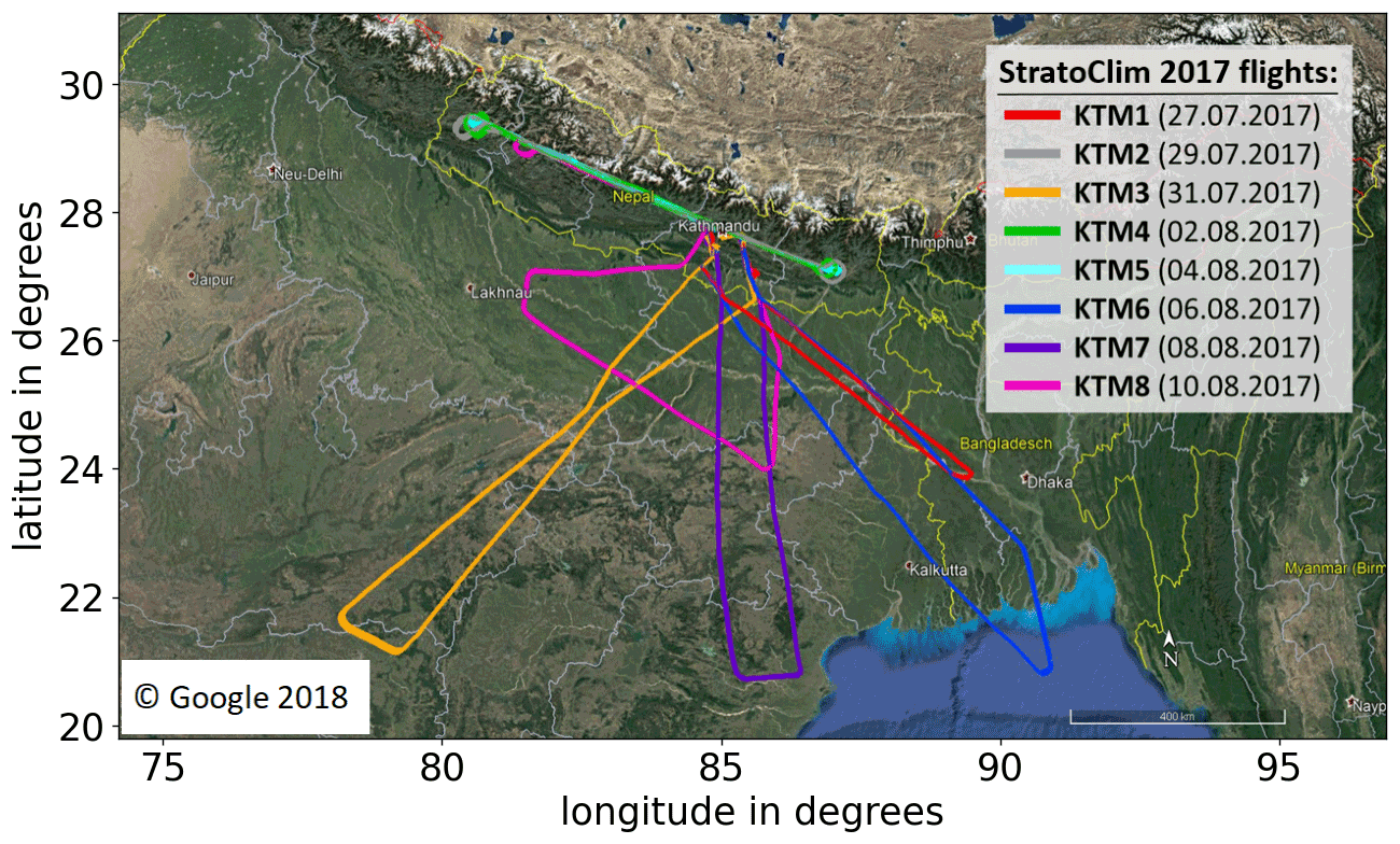
Figure 1 All flight paths of the mission flights conducted in Kathmandu (Nepal) as part of the StratoClim 2017 measurement campaign. GPS data from UCSE, © Google Earth 2018.

In this study, we also included measurements from the first phase of the StratoClim project which took place in 2016 in Kalamata, Greece (37^∘ N, 22^∘ E). During this campaign phase, three flights between 33–41^∘ N and 23–31^∘ E that reached up to 20 km altitude were conducted in the Mediterranean region (30 August, 1 and 6 September) using the M55 Geophysica. The geographical extent and the location of these flights relative to the strong subtropical potential vorticity (PV) gradient (von Hobe et al., 2021) indicate that these flights took place at the edge of the extratropics and the tropics. The results from these (here referred to as) extratropical aerosol measurements are juxtaposed to the tropical data from the ASM during StratoClim 2017.

3 Instrumentation on the M55 Geophysica high-altitude research aircraft

The main instrument used for the measurements discussed in this study is the UHSAS-A aerosol spectrometer (see Sect. 3.1). Besides the UHSAS-A, in situ and remote sensing instruments aboard the M55 Geophysica were included for the analyses discussed in this study: the COPAS (Sect. 3.2) and NIXE-CAS (Sect. 3.3) in situ particle detectors, the MAS backscatter probe (Sect. 3.4), the MAL airborne lidar (Sect. 3.5), and the COLD2 carbon monoxide instrument (Sect. 3.6). The meteorological parameters and the avionic data from the M55 Geophysica are provided by the Unit for Connection with Scientific Equipment (UCSE; Sokolov and Lepuchov, 1998). The potential temperature (Θ) is calculated from the UCSE-based temperature and pressure data as defined by the World Meteorological Organization (WMO, 1966). For the given vertical temperature and pressure distribution and for the Θ range covered during StratoClim 2017 (up to ∼477 K), the WMO-compliant Θ values do not deviate by more than ∼1 K from the results according to the recently reassessed Θ calculation (Baumgartner et al., 2020).

3.1 The UHSAS-A

The ultra-high sensitivity aerosol spectrometer – airborne (UHSAS-A) is the underwing version of the UHSAS (Cai et al., 2008), a laser-based aerosol spectrometer designed and manufactured by Droplet Measurement Technologies (DMT, Boulder, Colorado, USA). It is designed for airborne operation at altitudes of up to 12 km and is able to measure aerosol particle number size distributions in the diameter range from 65 nm to 1 µm at a 1 Hz sampling frequency.

For operations at altitudes of up to 20 km under tropical, stratospheric ambient conditions aboard the M55 Geophysica research aircraft, two major modifications of the commercially available version of the UHSAS-A were necessary: integrating a pressure sensor measuring the air pressure in the optical detection cell of the UHSAS-A and installing a new pump system enabling the maintenance of constant system flows even under low stratospheric air pressures. The stability of the sample, sheath, and purge flow was tested in a low-pressure chamber before the StratoClim 2017 field campaign. These low-pressure chamber tests were conducted under air pressure values down to 45 hPa within the UHSAS-A measurement cell. During the operation aboard the M55 Geophysica the sample, sheath, and purge flow were stable and constant throughout all StratoClim 2017 mission flights (Appendix A1). Additionally, the new dual-headed membrane pump system, installed in the UHSAS-A, minimizes the pulsation of the flow within the UHSAS-A measurement cell compared with a single-headed membrane pump. The sample flow measurement was characterized as a function of pressure. For this purpose, the UHSAS-A was located in the low-pressure chamber and connected through a chamber outlet via a high-precision needle valve to a reference flow meter (Gilibrator-2, SENSIDYNE; Appendix A1).

Prior to the 2017 StratoClim field campaign, the UHSAS-A was calibrated with polystyrene latex spheres (PSL, Thermo Fisher Scientific) with diameters of 102, 147, 296, and 799 nm. During the calibration process the PSL particles were selected by size with a differential mobility analyzer (DMA, TSI 3080 with TSI 3081) to remove doublets and contamination particles (Appendix A2). During the field campaign in Nepal, the calibration of the UHSAS-A was validated with the same PSL calibration standards without the DMA before every mission flight. The uncertainty of the measured number concentration was determined to be lower than 10 % based on laboratory characterization (Appendix A3). This is valid as long as the uncertainty due to counting statistics is also lower than 10 %. For the 1 Hz resolved measurements, this is the case for ambient particle number concentrations larger than 100 cm⁻³. At ambient particle number concentrations as low as 1 cm⁻³, the data should be averaged over time intervals of about 100 s to gain sufficient counting statistics. For a typical number of about 70 particle counts for a sampling interval of 1 s in the ATAL altitude range, this would result in an uncertainty of 12 %. However, due to missing in-line temperature measurements and the wide ambient temperature range during StratoClim (compared with the characterization in the laboratory), the total uncertainty of the UHSAS-A ambient number concentration and particle mixing ratio measurements was estimated to be up to 25 %.

3.2 COPAS

The COndensation PArticle counting System (COPAS) consists of two separate units, each containing two individual condensation particle counters. Three of the condensation particle counters detect aerosol particles with diameters larger than 6, 10, and 15 nm, respectively. Particles with diameters <1 µm were aspirated with almost 100 % efficiency and transported through the aerosol lines to the detector. The fourth condensation particle counter detects the aerosol particles with diameters larger than 10 nm, which have previously passed through a heated tube section (at 270 ^∘C) of about 1 m length. Therefore, this channel detects residual particle cores which are non-volatile at this temperature. The COPAS has been characterized in Weigel et al. (2009), and the application of the heated channel has been adopted for several studies (Curtius et al., 2005; Borrmann et al., 2010; Weigel et al., 2011, 2014, 2021a).

3.3 NIXE-CAS

The New Ice eXpEriment – Cloud and Aerosol Spectrometer with Detection of POLarization (NIXE-CAS-DPOL, here referred to as NIXE-CAS) is part of the New Ice eXpEriment Cloud and Aerosol Particle Spectrometer (NIXE-CAPS) underwing probe. Together with the Cloud Imaging Probe greyscale (NIXE–CIPg), the NIXE-CAPS can measure the particle size distribution for larger aerosol particles as well as cloud particles within a diameter range from 0.61 to 937 µm (Costa et al., 2017). The overall measurement uncertainties of the particle number concentrations and the particle sizing were estimated to be approximately 20 % by Costa et al. (2017). More detailed descriptions of the instrument performance and measuring principles are given by Baumgardner et al. (2017). For this study, the lowest size bins of NIXE-CAS (0.61 to 3 µm) provide additional information extending beyond the upper detection limit of the UHSAS-A, as such large aerosol particles potentially influence the derived backscatter ratios.

3.4 MAS

The multiwavelength aerosol scatterometer (MAS) is an elastic backscatter near-range lidar that operates at wavelengths of 532 or 1064 nm. It measures the backscatter and the depolarization from cloud and aerosol particles like a remote sensing lidar but in situ at a range of 3 to 30 m from the aircraft. It is capable of measuring at a time resolution of 5 to 10 s, which translates into a horizontal resolution of 1 to 2 km at the M55 Geophysica cruising speed of about 170 m s⁻¹. The detection limit of the aerosol backscatter coefficient for a single 10 s data point is $\mathrm{5}\times {\mathrm{10}}^{-\mathrm{10}}$ ${\mathrm{m}}^{-\mathrm{1}}{\mathrm{sr}}^{-\mathrm{1}}$. Its technical details and an analysis of its measurement performance aboard the M55 Geophysica are discussed in detail by Cairo (2004), Cairo et al. (2011), and Molleker et al. (2014).

3.5 MAL

The miniature aerosol lidar (MAL) aboard the M55 Geophysica is a combination of two identical stand-alone airborne lidar systems, one facing upwards and the other facing downwards. The two microjoule backscatter-depolarization lidar systems operate at a wavelength of 532 nm and are capable of measuring range-resolved backscatter and depolarization profiles along the aircraft flight track, 2 km above and underneath the aircraft. For a 900 s flight interval (at cruising speed of about 170 m s⁻¹) probing an atmospheric layer at 17 km altitude from a distance of ∼1500 m, the detection limit of the aerosol backscatter coefficient is $\mathrm{5}\times {\mathrm{10}}^{-\mathrm{10}}$ ${\mathrm{m}}^{-\mathrm{1}}{\mathrm{sr}}^{-\mathrm{1}}$. Previous applications of the MAL lidar are discussed in publications by Cairo (2004), Mitev et al. (2014), and Molleker et al. (2014). For the RECONCILE campaign, a comparison study between the MAL lidar aboard the M55 Geophysica and the satellite-borne CALIOP lidar was conducted by Mitev et al. (2012).

3.6 COLD2

During the 2017 StratoClim field campaign, the carbon monoxide (CO) mixing ratio was measured in situ by the COLD2 (Carbon Oxide Laser Detector 2), the newly improved version of the Cryogenically Operated Laser Diode spectrometer (COLD) aboard the M55 Geophysica. The previous version COLD, based on a lead salt laser, operating around liquid nitrogen temperature, has successfully been operated during several tropospheric and stratospheric measurement campaigns since 2005, and its functionality is described in detail by Viciani et al. (2008). The present instrument is based on a room temperature quantum cascade laser and updated electronics, with a substantial reduction in weight and dimensions, and no need for cryogenic fluids. The detection principle of the COLD instruments is based on tunable diode laser spectroscopy. During the 2017 StratoClim operation, the COLD2 instrument attained an in-flight sensitivity of 1 to 2 ppb with a time resolution of 1 Hz and an accuracy of 3 % (Viciani et al., 2018). In this study, the CO measurements are adopted as tracer for air masses affected by pollution or biomass burning.

4 The vertical distribution of the aerosol particle mixing ratio within the AMA

The identification of transport and nucleation processes (i.e., new particle formation – NPF) of aerosol particles in the UT–LS and their influence on the radiation balance and chemistry of the atmosphere requires the knowledge of the vertical distribution of the aerosol particle properties, such as particle size and number concentration. Figure 2a shows the vertical distribution of the particle mixing ratio (given in number of particles per milligram of ambient air) as measured by the UHSAS-A during all research flights of the StratoClim 2017 measurement campaign. The potential temperature (Θ) is used as the vertical coordinate. To ease the recognition of the variability between the individual flights, the measured particle mixing ratios (1 Hz temporal resolution) are marked using data points with different colors. The median of the particle mixing ratio of all eight measurement flights, calculated over 5 K potential temperature intervals, is plotted in black together with the 25th and 75th percentiles as horizontal bars for each median value. To avoid artifacts due to fewer particles at high altitudes, the median profile and the 25th and 75th percentiles were calculated based on the 1 Hz data for Θ<420 K and based on the resampled 0.1 Hz data set (see red dots in Fig. 3a) for Θ>420 K. For this, we have to assume that the atmospheric conditions remain quasi-homogeneous above 420 K within a 10 s interval (about 1.7 km flight distance). The number of 1 Hz data points included in each 5 K potential temperature interval is indicated in Fig. 2b, where each data point implies the measurement of a complete size distribution.

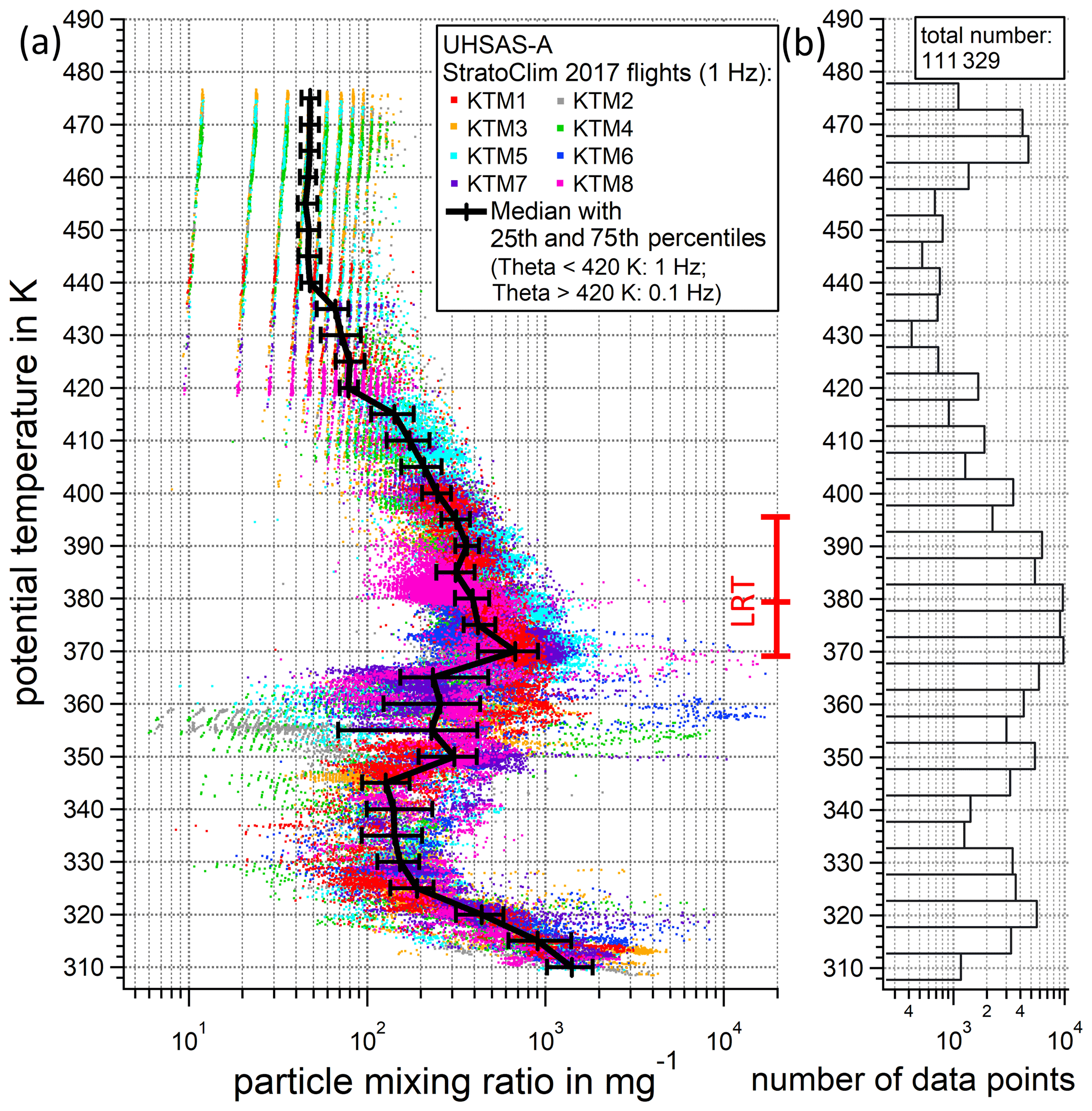
Figure 2 (a) Vertical profile of the particle mixing ratio measured with the UHSAS-A (diameter range of 65 nm–1 µm) during the StratoClim 2017 measurement campaign, with the potential temperature as the vertical coordinate. The 1 Hz resolved data points of the individual measurement flights are marked by individually colored dots. The median profile of all flights is plotted in black in steps of 5 K (each over a ±2.5 K interval) with the 25th and 75th percentiles, based on the 1 Hz data for Θ<420 K and on the 0.1 Hz data for Θ>420 K. The red vertical bar indicates the position (minimum, mean, and maximum Θ level) of the lapse rate tropopause (LRT; calculated from the ECMWF reanalysis data) during the campaign period. (b) The number of 1 Hz data points included in each 5 K potential temperature interval. Each 1 Hz data point covers a particle size distribution from 65 nm to 1 µm particle diameter.

From comparatively high particle mixing ratios (median of about 1500 mg⁻¹) close to the ground level (Θ=310 K), the particle mixing ratio decreases by an order of magnitude to about 150 mg⁻¹ up to a potential temperature of 330 K. As evident from the 1 Hz resolved data, particle mixing ratios of up to 10 000 mg⁻¹ are measured between 310 and 330 K. Up to the Θ level of 345 K, the median particle mixing ratio remains at about 150 mg⁻¹. The variability in the measurement results increases with Θ, which can be seen from the changes in the deviation of the 25th and 75th percentiles with respect to the median.

From 345 to 350 K potential temperature, the median value increases to a particle mixing ratio of 300 mg⁻¹ until it reaches a maximum of 700 mg⁻¹ at about 365 to 370 K potential temperature. Between 350 and 370 K, the 1 Hz data show a high variability in the particle mixing ratio, both between the different flights and when the flights are considered individually. Particle mixing ratios between 6 mg⁻¹ and over 10 000 mg⁻¹ were measured here. This high variability is also visible in the percentiles. Apart from the variability in the sampled air masses inherent in the dynamics of the AMA, causes for such variability may also be the occurrence of NPF events, convective outflow, and scavenging by the large persistent convective cloud systems. In these cloud systems, many aerosol particles are activated to form condensation nuclei of cloud droplets or get washed out by scavenging, resulting in the observed very low aerosol particle mixing ratios (Croft et al., 2010; Yang et al., 2015). On the other hand, these strong convective systems can lead to vertical transport of polluted air from the boundary layer, with elevated particle mixing ratios, up to high altitudes. A possible cause for the high particle mixing ratios in this altitude range, and sometimes up to 380 K potential temperature (flight KTM8), can also be NPF from precursor gases. These precursor gases of natural and anthropogenic origin are also subject to vertical transport by deep convective cloud systems reaching the TTL and cause NPF under favorable thermodynamic conditions (Borrmann et al., 2010; Höpfner et al., 2019; Weigel et al., 2021a, b). The lapse rate tropopause (LRT in Fig. 2a) during the 2017 campaign period was located between 369 and 396 K at a mean Θ level of about 380 K based on the European Centre for Medium-Range Weather Forecasts (ECMWF) ERA-Interim reanalysis data. Above the tropopause region, starting at about 380 K potential temperature, the variability in the particle mixing ratio decreases with increasing Θ.

Up to a potential temperature of 420 K, the median of the particle mixing ratio decreases to about 80 mg⁻¹, except for a local maximum at a potential temperature of 390 K. From there, up to a potential temperature of 440 K, the particle mixing ratio decreases further to a median of about 50 mg⁻¹. Up to about 475 to 480 K, the highest Θ levels reached during the StratoClim 2017 measurement campaign, the median of the particle mixing ratio remains between 40 and 50 mg⁻¹. Especially for potential temperatures larger than 420 K and low particle mixing ratios in the range from 10 to 100 mg⁻¹, it is noticeable that the 1 Hz data points form a vertical and slightly inclined, discrete stripe pattern towards larger particle mixing ratios. This is due to the poor counting statistics of the single 1 Hz data points at these concentrations in combination with the constantly regulated sample flow (of 50 cm³ min⁻¹). However, due to the high number of 1 Hz data points (about 400 to 4000) available for each 5 K interval, we were even able to resample the data set to a temporal resolution of 0.1 Hz in this Θ range and then calculate robust median values with the given Θ resolution.

For relating these UHSAS-A results to the particle mixing ratios observed in other tropical and subtropical UT–LS regions, two data sets from the tropics as well as two sets from the extratropics were selected. These measurements were conducted with the COPAS instrument (described in Sect. 3.2) during the 2016 StratoClim field campaign in Greece (extratropics) and StratoClim 2017 in Nepal (tropics), and as airborne measurements within the tropics and the extratropics published in Borrmann et al. (2010). One more data set from the tropics and the extratropics was digitized from Fig. 1 of the publication by Brock et al. (1995). Figure 3a shows the median profiles of the COPAS measurement series from the 2016 and 2017 StratoClim campaigns together with the median profile from the 2017 StratoClim UHSAS-A data set. In addition to the tropical and extratropical profiles from Brock et al. (1995), Fig. 3b compares the UHSAS-A and COPAS measured profiles from StratoClim 2017 (Nepal) with three further profiles measured by the COPAS instrument within the tropics during the SCOUT-AMMA 2006 (West Africa, red line), SCOUT-O3 2005 (northern Australia, pink dotted line), and TROCCINOX 2005 (Brazil, dark green dotted line) field campaigns, discussed by Borrmann et al. (2010) and Fierli et al. (2011).

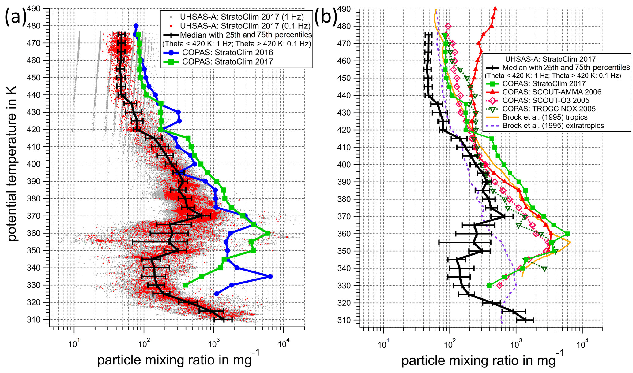
Figure 3 Vertical profile of the particle mixing ratio with the potential temperature as the vertical coordinate. Panel (a) shows the 1 Hz resolved particle mixing ratios measured with the UHSAS-A (diameter range of 65 nm–1 µm) during StratoClim 2017 as gray dots and the 0.1 Hz averaged particle mixing ratios as red dots. The median profile of all flights is plotted in black in steps of 5 K (each over a ±2.5 K interval) with the 25th and 75th percentiles, based on the 1 Hz data for Θ<420 K and on the 0.1 Hz data for Θ>420 K. The median profile of the particle mixing ratio measured by the COPAS (diameter range of 10 nm–1 µm) during the StratoClim 2016 measurement campaign in the extratropics (Kalamata, Greece) is shown in blue, and the profile measured during StratoClim 2017 (Kathmandu, Nepal) in the tropics is shown in green. Panel (b) includes the median profile (with the 25th and 75th percentiles) of particle mixing ratios measured with the UHSAS-A during StratoClim 2017 (black line); the median profiles measured by COPAS for particle diameters larger than 10 nm during StratoClim 2017 (Nepal, green line), SCOUT-AMMA 2006 (West Africa, red line), and SCOUT-O3 2005 (Australia, red dotted line); and for particle diameters larger than 6 nm during TROCCINOX 2005 (Brazil, green dotted line), as depicted in Borrmann et al. (2010). The median profiles, digitized from Fig. 1 in Brock et al. (1995), for the tropics are plotted as an orange line, and those for the extratropics are plotted as a dashed purple line.

In the region of the upper troposphere with potential temperatures between about 350 and 370 K, the median of the particle mixing ratio measured by COPAS during StratoClim 2017 (green line) reaches a maximum of 6000 mg⁻¹. A maximum (particle mixing ratio of up to about 6500 mg⁻¹) in this Θ range was also observed by Brock et al. (1995) in the tropical central Pacific (orange line). The median of the UHSAS-A measurement remains almost constant in this Θ range with significantly lower particle mixing ratio values of about 250 mg⁻¹. However, the variability in the particle mixing ratio measured by the UHSAS-A is, as discussed above, very high in this Θ range. The COPAS measurements shown here cover the particle diameter range from about 10 nm to 1 µm, the measurements of Brock et al. (1995) were from 8 nm to 3 µm, whereas the UHSAS-A detects aerosol particles in the diameter range from 65 nm to 1 µm. The difference in the particle mixing ratios between the median values of the COPAS and the UHSAS-A measurements of more than about 5500 mg⁻¹ shows that very small aerosol particles between 10 and 65 nm in diameter dominate the aerosol total particle mixing ratios. This indicates that especially the Θ range between 350 and 370 K is influenced by NPF, which has also been shown by Weigel et al. (2021a) and Weigel et al. (2021b).

During the ASM, between about 370 and 415 K potential temperature, the median profile of the UHSAS-A data (diameter of 65 nm to 1 µm) shows particle mixing ratios that are up to 2 times higher than the median profile observed by Brock et al. (1995) (diameter of 8 nm to 3 µm) in extratropical regions (see Fig. 3b). The median profile of the COPAS measurement during the StratoClim 2016 measurement campaign in Greece (blue line in Fig. 3a) also shows lower particle mixing ratios than the comparative measurement within the AMA region (green). Compared with the extratropical COPAS measurements from StratoClim 2016, the UHSAS-A vertical profile shows mostly lower particle mixing ratios. However, in contrast to the UHSAS-A, the measurements with the COPAS also include very small aerosol particles starting from 10 nm in diameter (or rather from 6 nm during TROCCINOX 2005). Thus, inside the AMA, higher particle mixing ratios were observed for the size diameter range from 65 nm to 1 µm at altitudes between roughly 370 and 415 K than during similar measurements in the extratropics which include even much smaller particles (starting from 8 nm; Brock et al., 1995). This enhanced aerosol mixing ratio can be associated with the ATAL discovered by Vernier et al. (2009), who observed the ATAL in about the same altitude range with potential temperatures between 370 and 420 K on the basis of satellite-borne lidar measurements. Figure 3b shows that such a maximum between roughly 340 and 390 K was also observed in the mixing ratios of fine-mode particles obtained from COPAS in other tropical locations (northern Australia, West Africa, and Brazil; Borrmann et al., 2010), albeit with significantly lower absolute values than for the AMA region. The increase in the particle mixing ratio for altitudes above the 420 K level over West Africa was explained by Borrmann et al. (2010) as the influence of the 2006 Soufrière Hills eruption in the Caribbean (also discussed by Prata et al., 2007 and Vernier et al., 2009). Figure 3a shows that a decrease in the mixing ratios detected with the UHSAS-A and COPAS from about 170 to 80 mg⁻¹ and from 470 to 170 mg⁻¹, respectively, can be seen between the 410 and 420 K potential temperature levels. The altitude levels of this decrease roughly coincide with the top of the 2017 AMA circulation system (von Hobe et al., 2021). Aloft, the particle mixing ratios are mainly controlled by the large-scale isentropic transport in the lowermost stratosphere and are less influenced by the AMA.

5 The vertical profile of the aerosol particle size distribution within the Asian monsoon anticyclone

Characterizing the ATAL, described by Vernier et al. (2011), requires knowledge about the vertical progression of the aerosol particle size distribution. Within UT–LS altitudes, this is also important for the analysis of NPF events, cloud formation, and transport processes as well as for the calculation of the radiative balance and parameters like aerosol volume concentration (Höpfner et al., 2019) and aerosol surface area, available for heterogeneous chemical conversion processes.

The results shown here are the first measurements made with an UHSAS-A in the tropical lower stratosphere (up to more than 20 km altitude over the Indian subcontinent). The performance of the modified UHSAS-A (see Sect. 3.1) has been thoroughly tested in the laboratory (as described in Appendix A). To put the in situ measurements at altitude into context with some of the other few available observations, a comparison was made with other optical particle counter measurements of the aerosol particle size distributions from the stratosphere.

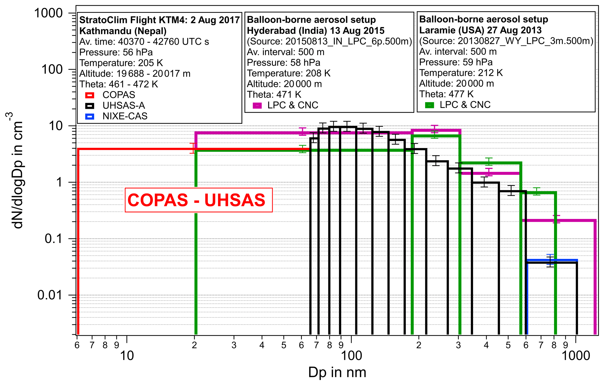
Figure 4 Aerosol particle size distribution combined from the measurements performed by the UHSAS-A, COPAS, and NIXE-CAS (overlapping size range with the UHSAS-A) for the highest flight level reached during the flight KTM4 of the 2017 StratoClim campaign. The particle number concentrations are given for ambient conditions. The concentration of the size bin marked in red (6 to 65 nm) is the difference between the total number concentrations measured by COPAS (diameter range of 6 nm to 1 µm) and UHSAS-A (diameter range of 65 nm to 1 µm). Air pressure, temperature, altitude, and potential temperature according to the UCSE data set are also shown. For comparison, measurements of the balloon-borne measurement setup described by Ward et al. (2014) and Campbell and Deshler (2014) for flights from Hyderabad (India) and from Laramie (USA) are shown in purple and green, respectively.

For this purpose, we chose two measurements conducted with a balloon-borne setup which continues the series of in situ data described in Deshler et al. (2003), Ward et al. (2014), and Deshler et al. (2019). The comparison measurements were from Hyderabad (India; 17.47^∘ N, 78.58^∘ E) in August 2015, also above the ATAL (Vernier et al., 2018) during the ASM period, and from Laramie (USA; 41.32^∘ N, 105.58^∘ W) in August 2013. The optical particle counters (LPC; laser particle counter) used for the measurements from Hyderabad and Laramie were operated with a particle diameter detection range from 0.18 to 32 µm and 0.18 to 9 µm, respectively. In both cases, total particle concentration measurements were made with a condensation nuclei counter (CNC) with a nominal detection diameter of 20 nm (Campbell and Deshler, 2014), flown in parallel with the LPCs. In Fig. 4, the resulting particle size distributions are compared with the data from the UHSAS-A obtained at the highest flight level (56 hPa pressure level) of the StratoClim mission flight KTM4. This size distribution was combined with the COPAS data for an additional size bin between 6 and 65 nm. The overlapping size bin of the NIXE-CAS measurements is shown in blue and agrees well with UHSAS-A data within the uncertainties. In each case, the balloon data set (500 m vertical averaging interval) was chosen for which the altitude range corresponded mostly to the flight level of the M55 Geophysica during the UHSAS-A measurements.

For the comparison of these data sets, the higher size resolution of the UHSAS-A and the difference in the detection range compared with the balloon-borne instrumentation as well as the temporal and spatial distance between these measurements must be taken into account. Additionally, the size distribution measured during StratoClim 2017 is reported with the bin limits resulting from the calibration with PSL particles (refractive index m=1.59; see Appendices A2 and A4), while the balloon-borne measurements were corrected for a refractive index of 1.45.

The ambient total number concentration for the observation from StratoClim 2017 of ∼9 cm⁻³ is slightly lower than the 10 cm⁻³ observed over Hyderabad but one-third larger than the 6 cm⁻³ measured at Laramie. For a better quantitative comparison of the size distributions, the integrated surface area (dS) and volume concentrations (dV) were calculated. For the measurements during StratoClim 2017, these values were calculated using the original bin sizes and the ones recalibrated for a refractive index of m=1.45. In both cases, for the StratoClim 2017 observation, the values for dS≈0.44 µm² cm⁻³ (0.52 µm² cm⁻³ for m=1.45) and dV≈0.021 µm³ cm⁻³ (0.029 µm³ cm⁻³ for m=1.45) are smaller than the measurements from Hyderabad and Laramie, with dS≈0.79 µm² cm⁻³ and dV≈0.05 µm³ cm⁻³ observed at both locations. Compared with the balloon-borne measurements from Hyderabad, these lower values for total particle number, surface area, and volume concentration observed during StratoClim 2017 also agree with a lower backscatter ratio (BR) signal observed by CALIOP at this altitude during StratoClim 2017. During July and August 2015, CALIOP observed a BR of about 1.07 at ∼20 km altitude within ±5^∘ latitude and ±30^∘ longitude around Hyderabad (Vernier et al., 2018), while the BR measured by CALIOP during StratoClim 2017 at 20 km was below 1.05 (Sect. 6.2).

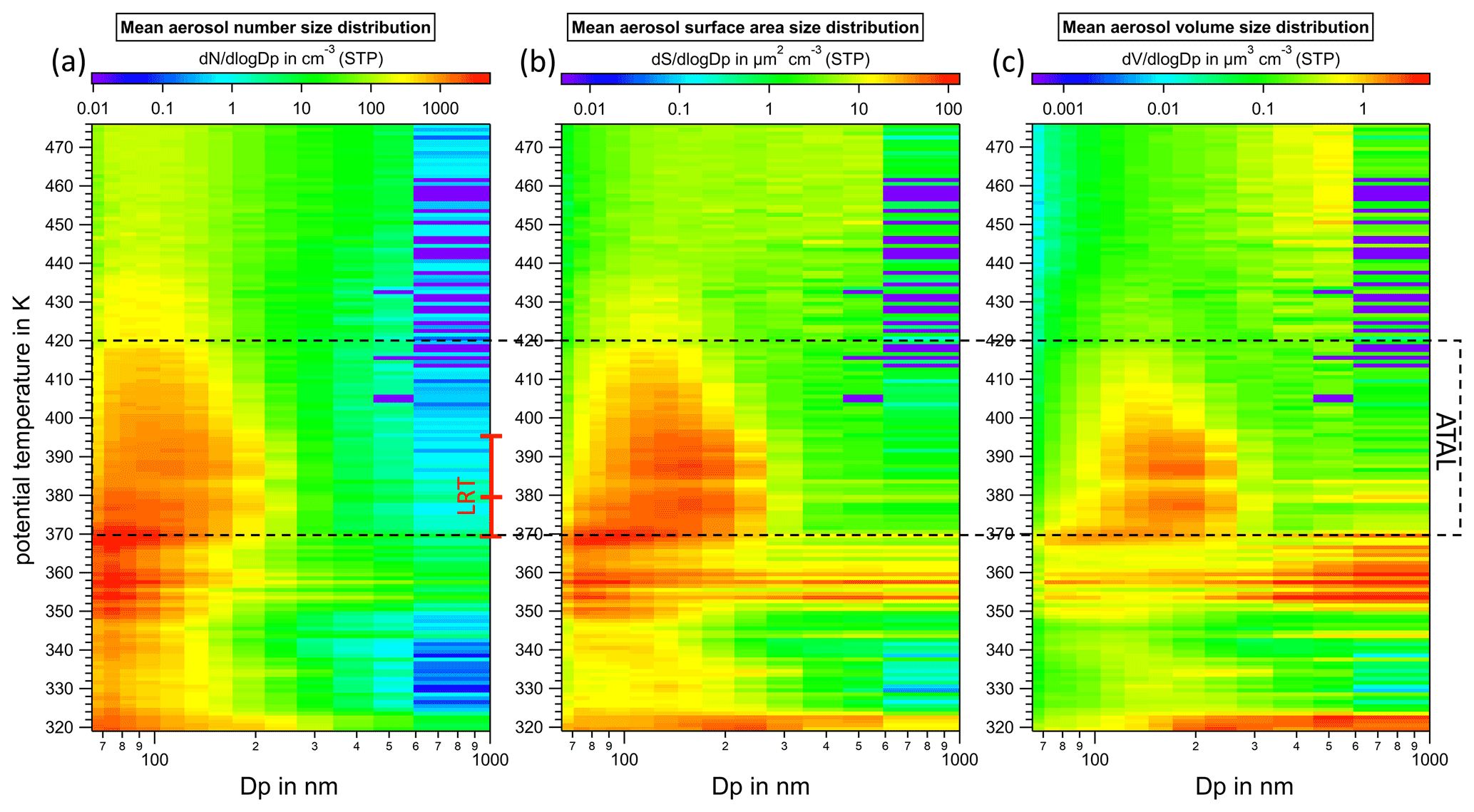
Figure 5 Vertical profile of (a) the aerosol particle number size distribution, (b) the aerosol particle surface area size distribution, and (c) the aerosol particle volume size distribution measured by the UHSAS-A during the 2017 StratoClim field campaign averaged over 1 K potential temperature intervals. The color-coded concentrations for each size bin are converted from ambient conditions to standard temperature and pressure (STP). The red vertical bar indicates the position (minimum, mean, and maximum Θ level) of the lapse rate tropopause (LRT; calculated from the reanalysis data) during the campaign period. The vertical region of the ATAL is indicated with black dashed lines.

Figure 5 shows the vertical profile of the aerosol number size distribution (Fig. 5a), surface area size distribution (Fig. 5b), and volume size distribution (Fig. 5c) measured by the UHSAS-A averaged over the full StratoClim 2017 campaign period. The profiles were averaged with a vertical resolution of 1 K potential temperature. The concentrations for the distributions' diameter bins are color coded and normalized according to the bin widths in terms of dN $/$ dlogDp, dS $/$ dlogDp, and dV $/$ dlogDp. To be able to compare the measured concentrations of the number, surface area, and volume size distributions over the full altitude range, the ambient concentrations have been converted to standard temperature and pressure (STP; T₀=273.15 K; p₀=1013 hPa) using the ambient temperature and pressure measurements reported by the UCSE.

Starting at a Θ level of 320 K, the profile of the aerosol particle number size distribution (Fig. 5a) has a pronounced maximum at the lower end of the UHSAS-A detection size range (diameter between 65 and 80 nm) as well as enhanced number concentrations for the large aerosol particles with diameters of up to 1 µm. Until about 326 K potential temperature, the size distribution's maximum is located between particle diameters of 70 and 80 nm and the overall number concentration decreases. This is especially the case for particles with a diameter larger than 600 nm. Up to potential temperatures of about 350 K, the overall shape of the size distribution remains mostly constant. In the Θ range between 350 and 370 K, the aerosol size distribution is very variable. It also shows high number concentrations for large particles up to 1 µm in diameter, which are at the upper detection size range of the UHSAS-A, and a very pronounced Aitken mode. Above 370 K potential temperature, the main mode of the size distribution broadens and shifts its maximum to diameters of about 100 nm. This shift of the distributions main mode to larger particles is even more prominent in the surface area (Fig. 5b) and volume size distribution (Fig. 5c). This increase in aerosol surface area can have a local effect on heterogeneous chemical processes. Additionally, Yu et al. (2017) reported, based on model simulations, that these particles spread throughout the entire Northern hemispheric lower stratosphere, contribute about 15 % to the stratospheric column aerosol surface area in the Northern Hemisphere annually, and set a lower limit of the ASM contribution to the global stratospheric aerosol surface area of about 7 %. At about 395 K potential temperature, the concentrations, especially for larger particles, begin to decrease. Above 420 K, until the maximum ceiling during StratoClim 2017, the shape of the aerosol size distribution shows only low variability. Altogether, the measured vertical profiles of the aerosol size distributions for the 2017 AMA show the presence of an ATAL feature between approximately 370 and 420 K with the peak of the size distributions in the 80 to 300 nm diameter range.

6 Backscatter properties of the ATAL – results from in situ and remote sensing instruments

The ATAL was discovered as an enhancement of the newly reanalyzed and cloud-filtered backscatter ratio (BR) signal from the CALIOP lidar aboard the Cloud-Aerosol Lidar and Infrared Pathfinder Satellite Observations (CALIPSO) satellite (Vernier et al., 2009; Vernier et al., 2011). Vernier et al. (2015), Yu et al. (2017), Brunamonti et al. (2018), and Vernier et al. (2018) confirmed this enhancement using balloon-borne in situ backscatter and aerosol particle number concentration measurements. To undertake a comparison with these observations, we calculated the BR based on the in situ aerosol particle size distributions from the StratoClim 2017 campaign and compared it with the cloud-filtered CALIOP, MAS (Sect. 3.4), and MAL (Sect. 3.5) measurements for a mostly overlapping time period in 2017.

6.1 Method

For this analysis, all eight measurement flights from the StratoClim 2017 campaign are divided into segments of 100 s. Segments in which cloud particles have been detected by the NIXE-CAS are removed from the data set to be consistent with the cloud-filtered CALIOP, MAS, and MAL data sets. To ensure a high vertical resolution, flight segments with ascending or descending rates which result in a potential temperature rise or drop of more than 5 K per 100 s of flight time are also removed.

For each remaining 100 s interval, an averaged aerosol size distribution was calculated from the UHSAS-A measurements. The size range of these size distributions is extended from 65 nm–1 µm to 10 nm–3 µm using measurements conducted by the COPAS (Sect. 3.2) and NIXE-CAS (Sect. 3.3) instruments.

One size bin from 10 to 65 nm in diameter was calculated by subtraction of the UHSAS-A measured total number concentration (particle diameter range of 65 nm–1 µm) from the particle number concentration measured by the COPAS N₁₀ channel (particle diameter range of 10 nm to about 1 µm) described in Sect. 3.2. The measurements conducted by the NIXE-CAS instrument (see Sect. 3.3) extend the size distribution for large aerosol particles by one size bin with diameters of up to 3 µm. This way, as composite, the largest possible aerosol particle diameter range is covered with measurements that can be achieved from all of the Geophysica instruments. One example of this combined 100 s averaged aerosol size distributions is shown in Fig. 6.

Figure 6 Aerosol particle size distribution measured within the ATAL during flight KTM5 of the 2017 StratoClim measurement campaign. Combined out of the measurements conducted by the COPAS (red size bin), the UHSAS-A (black size bins), and the NIXE-CAS (blue size bins).

The backscatter ratio (BR) is calculated using Eq. (1) with the aerosol backscatter coefficient β_ap and the molecular backscatter coefficient β_mol:

$$\begin{array}{}\text{(1)}& {\displaystyle }{\displaystyle }\text{BR}={\displaystyle \frac{{\mathit{\beta }}_{\text{ap}}+{\mathit{\beta }}_{\text{mol}}}{{\mathit{\beta }}_{\text{mol}}}}.\end{array}$$

For every 100 s averaged aerosol size distribution, the aerosol backscatter coefficient β_ap is calculated based on the Mie theory, as comprehensively described in Cairo et al. (2011). Accounting for the aerosol chemical composition (Höpfner et al., 2019, observed the presence of ammonium nitrate particles), these calculations use a refractive index of 1.5 for the size distributions measured within the ATAL altitude region up to 420 K potential temperature. At Θ levels higher than 420 K, a refractive index of 1.45 is used, which better reflects the stratospheric aerosol properties. The bin limits of the UHSAS-A measured size distribution were recalibrated for the respective refractive index prior to the calculation of the backscatter coefficient (see Appendix A4 and Table A1). A sensitivity study (Appendix B) showed that the variation in the calculated aerosol backscatter coefficient is below 50 % for diameter shifts of the size distribution of ±10 % or for a variation in the refractive index of ±0.05. Additionally, black carbon particles might alter the result of the backscatter calculations, due to their complex refractive index and the uncertainties in their size representation in the particle size distribution measured by the UHSAS-A (see Appendix A2). Even though the presence of black carbon particles in the ATAL altitudes is enhanced during the ASM season, its contribution to the overall aerosol particle mass concentration (for particle diameters <2.5 µm) is reported to only be about 1.3 % at the 100 hPa pressure level (Gu et al., 2016). Moreover, the effect of the particles' hygroscopicity on the measured particle sizes and the resulting calculated backscatter compared with the remotely sensed backscatter, which is measured at ambient relative humidity, can not be ruled out.

To be able to compute the backscatter ratio, the molecular backscatter coefficient β_mol for each averaging interval is calculated. Based on Collis and Russell (1976), the simplified method from Cairo et al. (2011) is used along with the temperature and pressure measured by the UCSE system aboard the M55 Geophysica. To be able to compare the resulting BR values with the BR measured by CALIOP, MAS, and MAL, β_ap and β_mol are calculated using a wavelength of 532 nm.

6.2 Comparison between backscatter ratios obtained from in situ and remote sensing data

For a direct comparison between the in situ aerosol size-distribution-based BR and the BR measured by the satellite-borne CALIOP lidar, a CALIOP data set is needed that was measured within a comparable time period and in about the same geographical region as the StratoClim 2017 flight missions. Over the time period from 5 to 31 August 2017 (no CALIOP data are available in this region for the earlier part of the campaign period), a vertical profile of the BR at a wavelength of 532 nm measured by CALIOP was averaged between 15–45^∘ N and 70–100^∘ E (311 100 profiles included). This temporal and horizontal averaging is needed to increase the signal-to-noise ratio. To be able to detect the ATAL, the CALIOP data set was reanalyzed based on the CALIOP Level 1 V4.10 data set and calibrated between an altitude of 36 and 39 km, as previously described by Vernier et al. (2009). During this data processing, backscattering due to ice cloud particles was removed by applying a filter for the volume depolarization ratio within a pixel greater than 5 % (Vernier et al., 2011, 2015). The vertical profile was then averaged with a vertical resolution of 200 m. Additionally, vertical profiles of the BR at a wavelength of 532 nm measured by the MAS and MAL instruments aboard the M55 Geophysica were averaged over all StratoClim 2017 flight missions. As for the CALIOP data set, a cloud filter was applied to the MAS and MAL data sets. This filter excludes data points with a depolarization ratio greater than 5 % and BR values greater than 1.3 for the MAS and greater than 1.4 for the MAL.

Figure 7 shows the averaged CALIOP BR profile (represented by the red line) in an altitude range from 11 to 21 km. The BR calculated based on the in situ measured aerosol size distributions for the 100 s time segments (described in Sect. 6.1) is shown as blue dots. The blue line is the averaged profile for the size-distribution-based BR with a vertical averaging interval of 500 m and with the standard deviation represented by blue horizontal bars (shown for the MAS, MAL, and CALIOP BR profiles in Fig. C1). The mean BR profiles measured by the MAS and the MAL are given as green and orange lines, respectively.

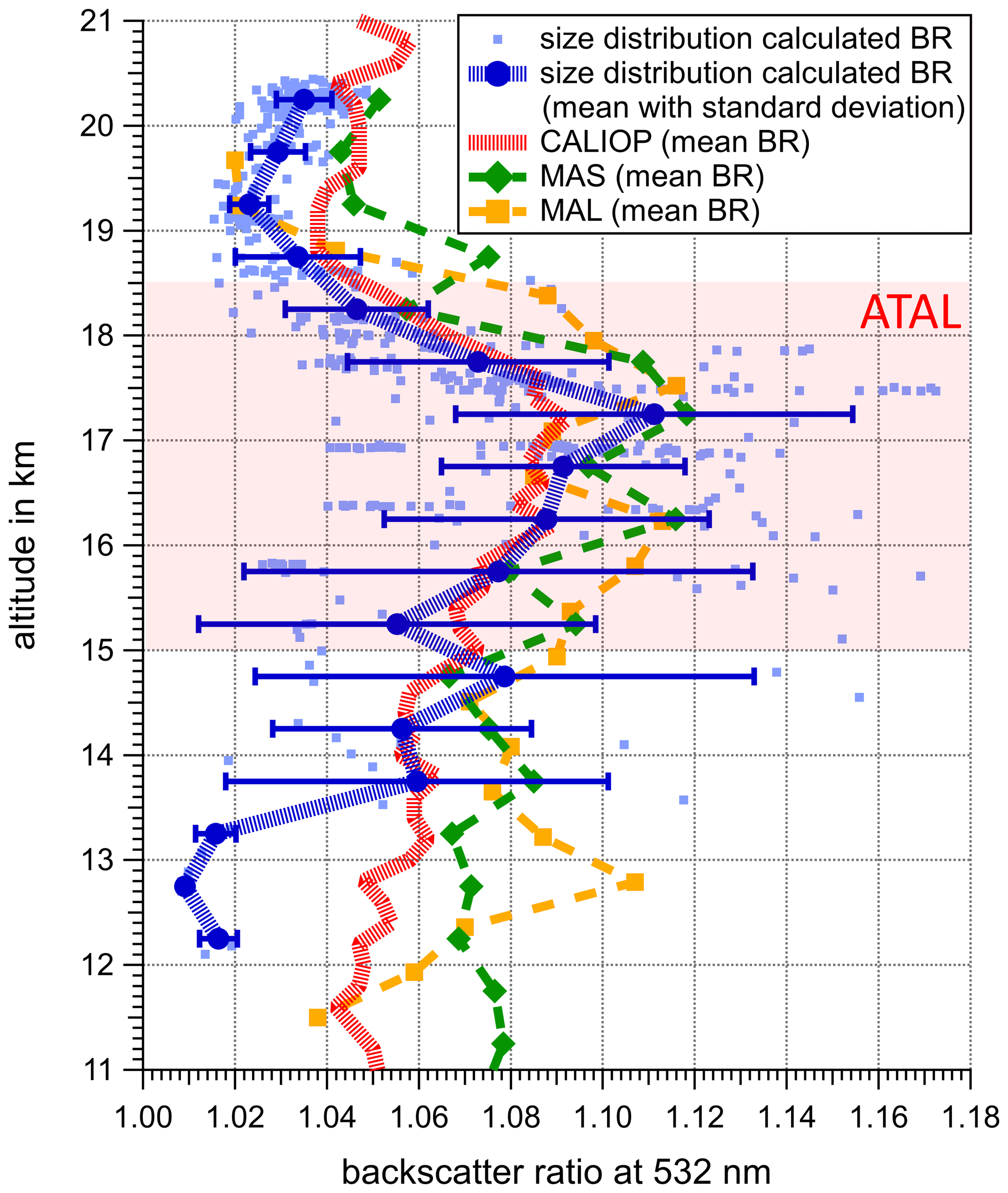
Figure 7 Vertical profile of the backscatter ratio at a 532 nm wavelength, calculated based on the aerosol size distributions measured during the 2017 StratoClim measurement campaign (blue dots, 100 s averages), showing the mean profile (blue line) and the standard deviation (blue bars). The mean profiles of the backscatter ratio at a 532 nm wavelength measured by CALIOP, MAS, and MAL are plotted in red, green, and orange, respectively.

At altitudes lower than 13.5 km, the size-distribution-based BR profile shows smaller values than the CALIOP, MAS, and MAL profiles. This can be explained by the frequent appearance of clouds in combination with the fast descent and ascent rates of the M55 Geophysica in this altitude range. Considering the selection criteria for the 100 s time segments described in Sect. 6.1, this leads to only a few valid data points in this altitude range. Additionally, the flight segments that are not directly associated with clouds could have been affected previously by scavenging of aerosol particles due to in-cloud processes (Croft et al., 2010; Yang et al., 2015) that have occurred prior to the observations. The local maximum in the BR profile measured by the MAL in this altitude range might also be considered as an artifact from cloud particles that could not be removed from the signal.

Between 13.5 and about 19 km altitude, the BR for the 100 s flight segments scatters around the CALIOP, MAS, and MAL mean profiles with values between 1.01 and over 1.17. Above 14 km altitude, its mean BR (blue line) increases from 1.06 parallel with the CALIOP profile (red line) to the maximum of the mean BR of more than 1.11 at altitudes between 17 and 17.5 km. Here, CALIOP, MAS, and MAL also observed the BR maximum. The aerosol size distribution shown in Fig. 6 was measured in this altitude range at about 17.5 km and a potential temperature level of 385 K. This 100 s averaged size distribution leads to a calculated BR of about 1.14. Above this maximum, the BR mean profile from the size-distribution-based calculations and the CALIOP measurements decrease mostly in parallel until 19 km altitude. Between 19 and 21 km altitude, the BR of both profiles begins to increase again. Here, the profiles measured by the MAS and the MAL instruments show the same behavior with a trend toward higher BR values. This increase in BR is consistent with the lower part of the Junge layer (Junge et al., 1961; Vernier et al., 2015). Within the overall picture and considering the standard deviation (blue bars), all four independent methods largely agree with one another. This confirms the ATAL as a layer of enhanced BR, while the altitude range of this observed aerosol layer also agrees very well with the ATAL altitudes between about 14 and 18 km, observed by Vernier et al. (2009), Vernier et al. (2011), Vernier et al. (2015), Brunamonti et al. (2018), and Vernier et al. (2018). The regional total sky radiative forcing caused by the ATAL has been reported (Vernier et al., 2015) to be around −0.1 W m⁻² since the late 1990s, which corresponds to one-third of the reported total radiative forcing (0.3 W m⁻²) from the global carbon dioxide increase during the same time period (Vernier et al., 2018).

6.3 ATAL variability during the StratoClim 2017 campaign period

Bucci et al. (2020) characterized the StratoClim 2017 campaign period as less convectively active than typically expected during that time of the ASM. They also showed that the second half of the campaign period was more influenced by convection compared with the first half. For this reason, we take a closer look at the differences in BR within the ATAL altitude range during the first and the second half of the campaign period. The backscattering of the size-distribution-based BR values shows the highly variable nature of the ATAL in time and space. This high variability in the ATAL, even on a day-to-day basis, was also reported by Hanumanthu et al. (2020) from balloon-borne backscatter measurements conducted during the ASM season 2016. In Fig. 8, the mean profiles of the BR derived from the in situ measured size distributions over the full campaign period (blue line), the first four flight missions (green dashed line), and the last four flight missions (orange dashed line) of StratoClim 2017 are shown. The mean profile is only displayed as a line if the corresponding altitude interval includes more than one data point (each resulting from a 100 s averaged size distribution). The red line in Fig. 8 represents the CALIOP BR profile for the same time period as discussed in the previous section (5 to 31 August 2017).

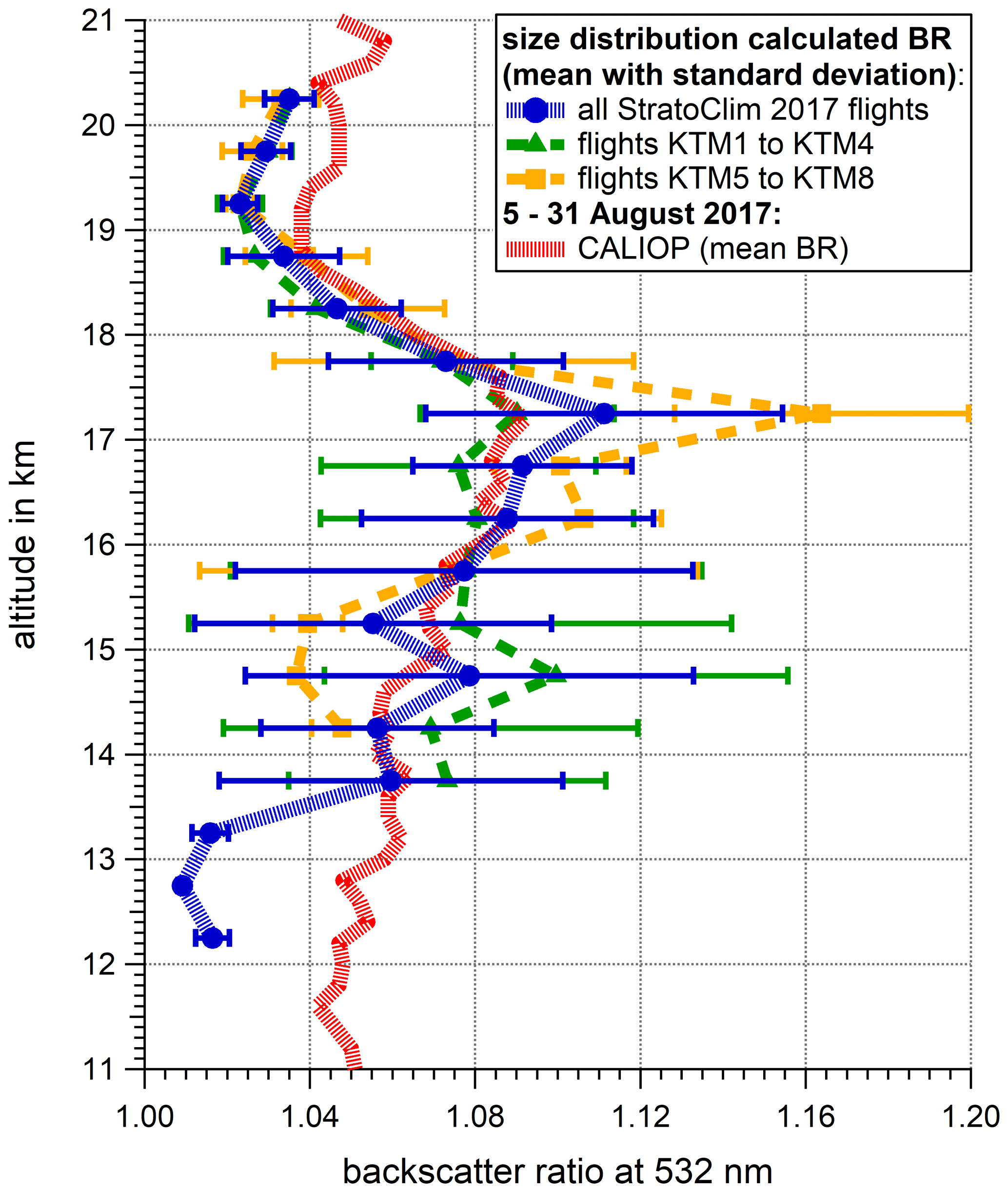
Figure 8 Vertical mean profile of the backscatter ratio at a 532 nm wavelength, calculated based on the aerosol size distributions measured during the 2017 StratoClim measurement campaign with the standard deviation shown as horizontal bars. The full period of the 2017 StratoClim field campaign is shown in blue, the first half of the campaign period is shown in green (flights KTM1 to KTM4), and the second half of the campaign period is shown in orange (flights KTM5 to KTM8). The red line represents the vertical mean BR profile measured by CALIOP between 5 and 31 August 2017.

During the first four mission flights up to 17 km, the mean profile of the aerosol size-distribution-based BR stays at values between about 1.07 and 1.08, except for a peak between 14 and 15 km altitude. The BR values of the individual 100 s segments still scatter widely in this altitude range, leaving the CALIOP mean profile for the time period from 5 to 31 August 2017 well in the range of the standard deviation (green bars). Between 17 and 17.5 km, the mean profile maximum for the first half of the campaign period matches the maximum of the CALIOP measured BR of about 1.09 to 1.1.

Due to the more frequent occurrence of convection during the second half of the campaign period, there are fewer cloud-free flight segments at altitudes of up to ∼15 km. However, above that altitude, the BR calculated based on the in situ measured aerosol size distributions are significantly higher compared with the first four campaign mission flights. Between 16 and 17.5 km altitude, its mean profile exceeds the CALIOP BR profile and has a pronounced maximum layer between 17 and 17.5 km altitude. Here, the size-distribution-based BR mean profile has a maximum BR between 1.16 and 1.17 compared with about 1.09 of the CALIOP mean profile (5 to 31 August 2017). In summary, the direct intercomparison between long time averages of the satellite data and small sets of individual research flights is generally a difficult task. For the ATAL in the ASM season of 2017, however, the juxtaposition of the respective measurements shows that the properties derived from the in situ particle size distributions can be broadly reconciled with the satellite observations.

6.4 The relation of the ATAL to CO and the AMA-centered equivalent latitude

The previous section shows that the intensity of the convective influence has an impact on the characteristics of the ATAL, here discussed in terms of the BR. A commonly used tracer for convective influences on the UT–LS region is an enhancement of the CO mixing ratio (Park et al., 2009; Pan et al., 2016). Here, one has to consider the different timescales of the transport and dilution processes of CO within the UT–LS (tens of days) and aerosol-related processes like coagulation and cloud scavenging that can have a significant impact within hours. Furthermore, between June 2006 and August 2008, Vernier et al. (2015) observed a seasonal dependence between the enhanced BR (measured by CALIOP between 14 and 18 km altitude) and an enhancement of the mean CO mixing ratio near the 100 hPa pressure level, as detected by the satellite-borne Microwave Limb Sounder (MLS, V2.21). They found that the aerosol peak in August lagged the CO peak by about 1 month during the investigated time period.

Figure 9a–c show the relationship between the in situ size-distribution-based aerosol BR (100 s flight segments) and the averaged CO mixing ratio measured by the COLD2 instrument (described in Sect. 3.6) over the full StratoClim 2017 campaign period, and its first half and second half, respectively. For both parts of the campaign, values of the BR larger than 1.05 are generally associated with CO mixing ratios larger than 40 ppb. The flight segments with CO mixing ratios lower than 40 ppb have all been associated with potential temperature levels larger than 420 K (color coded), which are close to or above the top of the AMA-caused confinement at about 420 to 440 K (Brunamonti et al., 2018; von Hobe et al., 2021). However, especially Fig. 9c shows that the highest CO mixing ratios are not necessarily correlated with a high BR. The highest values for the BR (larger than 1.14) encountered during the first four flights are accompanied by CO mixing ratios between 70 and 90 ppb and for the last four flights in the range of 50 to 70 ppb.

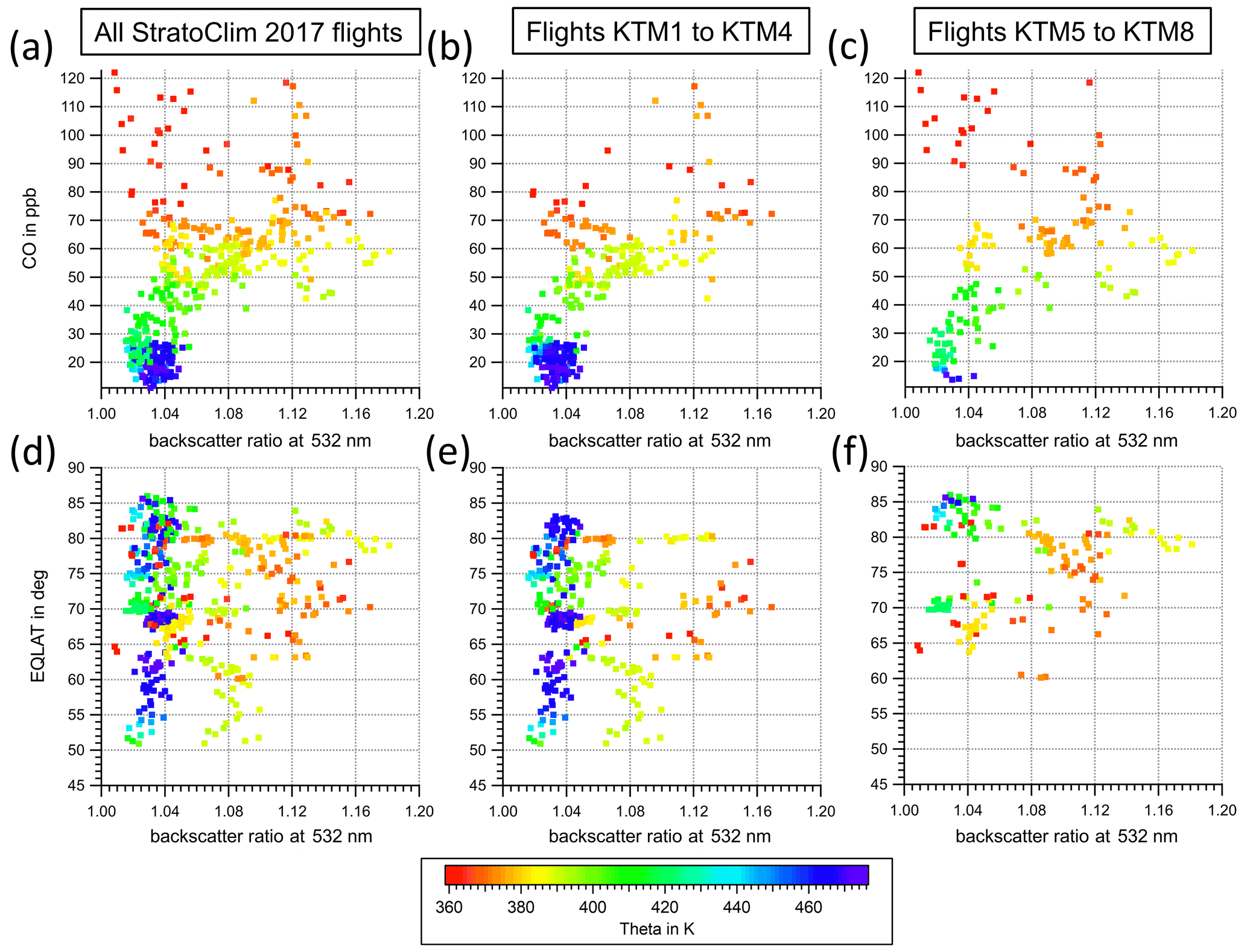
Figure 9 Scatterplots of the size-distribution-based BR with the CO mixing ratio (a–c) and the AMA-centered equivalent latitude (EQLAT) (d–f). Panels (a) and (d) represent the full period of the 2017 StratoClim field campaign, panels (b) and (e) represent the first half of the campaign period (flights KTM1 to KTM4), and panels (c) and (f) represent the second half of the campaign period (flights KTM5 to KTM8). The potential temperature is color coded.

Besides the strong convective vertical transport associated with the ASM, another feature of the ATAL should be considered, namely the confinement of its air masses within the AMA. This confinement can lead to an accumulation of aerosol particles and trace gases within the AMA region. One measure to relate the geographical position of our soundings to the position of the AMA core and its edge is the AMA-centered equivalent latitude (EQLAT). The center of the AMA is defined by the lowest values of the potential vorticity (PV) on the 380 K potential temperature level. An equivalent latitude for which 90^∘ N corresponds to the center of the AMA was projected for a closed PV contour according to Ploeger et al. (2015). It has to be noted that the definition of the EQLAT is only valid for a layer of about ±10 K around the 380 K isentrope, as PV contours in the AMA region are frequently not closed outside of this range. Furthermore, Ploeger et al. (2015) found that the edge of the confinement caused by the AMA can be determined from a local maximum in the gradient of PV along the 380 K isentrope and is on average located at around 65^∘ EQLAT. The EQLAT is calculated based on the ECMWF ERA-Interim reanalysis.

Figure 9d–f show the relationship between the EQLAT and the BR (full campaign period, first half, and second half, respectively). While there is no direct correlation between the BR and the EQLAT, high values of BR (larger than 1.1) only occur for flight segments with an EQLAT larger than 63^∘, for the first half of the campaign period (Fig. 9e). During the second half of the StratoClim 2017 campaign, BR values larger than 1.1 were only detected during flight segments with an EQLAT larger than 66^∘. This matches well with the edge of the AMA confinement at about 65^∘ EQLAT described by Ploeger et al. (2015). At high Θ levels above about 420 K (blueish colors), the BR values are always lower than 1.05. This shows that typically elevated ATAL BR values during the ASM could only be observed horizontally and vertically within the confinement of the AMA.

7 Conclusions

During the 2017 StratoClim field mission in the Asian summer monsoon (ASM) season, aerosol measurements were performed over Central Asia up to 20 km altitude aboard the M55 Geophysica research aircraft inside and above the Asian monsoon anticyclone (AMA) and the Asian tropopause aerosol layer (ATAL). Here, for the first time, submicrometer-sized aerosol size distributions were measured in situ down to a 65 nm particle diameter by a modified UHSAS-A optical particle counter. These measurements were conducted in conjunction with condensation particle counters (COPAS) and two near-range remote sensing instruments, MAS and MAL.

The ATAL BR observations by CALIOP during the StratoClim 2017 campaign period, as discussed in studies such as Vernier et al. (2009), Vernier et al. (2011), and Vernier et al. (2018) for previous and recent ASM seasons, were validated by calculating the BR based on the in situ aerosol size distributions as well as the BR directly measured by the MAS and MAL instruments. These four independent methods largely agree with one another and can confirm the ATAL as a layer of enhanced BR within an altitude range from 15 to 18.5 km. The maximum of the ATAL BR signal was observed at 17.5 km altitude, consistently by all four methods. The importance of the ATAL for the Earth's radiative budget was already underlined by Vernier et al. (2015), who reported that the regional total sky radiative forcing caused by the ATAL has been around −0.1 W m⁻² since the late 1990s. Furthermore, the in situ measurements show that the ATAL is highly variable in time and space and is not a closed, persistent layer. While there is a seasonal correlation between the CO mixing ratio and the ATAL (Vernier et al., 2015), no direct correlation on the smaller scale, between co-located in situ measurements of the CO mixing ratio and the size-distribution-based BR, could be found. However, values of BR that are typically elevated within the ATAL could only be observed for CO mixing ratios larger than 40 to 50 ppb. This is also consistent with the observations that enhanced BR values could only be observed within the confinement of the AMA at an equivalent latitude (EQLAT) larger than 63^∘ and below its top of confinement (at about 420 K potential temperature) during the StratoClim 2017 campaign period. This regional limitation of the ATAL with respect to the dynamics of the AMA is in good agreement with the horizontal (Ploeger et al., 2015) and vertical (von Hobe et al., 2021) limitations of the AMA-caused confinement.

From an experimental perspective, the ATAL is a fairly elusive, highly variable layer situated between approximately 370 and 420 K potential temperature or about 15 to 18.5 km altitude. Its lower part is close to – if not still inside – the highest region of convective outflows, whereas its upper part can be found at tropopause levels (between 369 and 396 K during StratoClim 2017) or slightly above. Thus, the aerosol of the upper ATAL part is subject to very slow vertical ascent (with rates of about 1 K potential temperature per day, as reported by Vogel et al., 2019, and von Hobe et al., 2021). At the same time, the lower part of the ATAL can be affected by rapid turbulent mixing which provides precursor gases and aerosols originating from the lower troposphere. In this complex dynamical setting, microphysical processes like new particle formation (NPF), aging by coagulation and condensational growth, and removal by scavenging act on the aerosol. The vertical profile of the measured aerosol particle size distributions in combination with the vertical profiles of the particle mixing ratios from the UHSAS-A and COPAS show a pronounced Aitken mode between the 350 and 370 K potential temperature levels, i.e., beneath the lower edge of the ATAL. With increasing altitude, the aerosol size distribution's main mode shifts towards the accumulation mode. This goes along with an increase in aerosol surface area, which might have a local effect on heterogeneous chemical processes and additionally contributes to the global stratospheric aerosol surface area (Yu et al., 2017).

Using simple box model simulations (adopting the SOCOL – SOlar Climate Ozone Links; Stenke et al., 2013 – coagulation subroutines), Weigel et al. (2021a) showed that the freshly nucleated aerosol particles (as observed from COPAS) coagulate onto the background aerosol (as observed by the UHSAS-A) within a few hours. The short periods of time available to detect recent NPF events and the still frequent NPF encounters during StratoClim 2017 (detected by COPAS) indicate the prevalence of such events within the ASM region (Weigel et al., 2021a, b). Still, these simulations suggests that the coagulation of freshly nucleated aerosol particles alone cannot cause the lower part of the aerosol size distribution as measured by the UHSAS-A inside the ATAL altitude range. Furthermore, the question of where the particles larger than roughly 500 to 800 nm in the UHSAS-A size distributions come from remains open. Condensational growth could be a major process, although the nature and amounts of the various possible condensable gases are not yet well known. Furthermore, the upward transport of already existing larger aerosol particles (Yuan et al., 2019) can contribute to the overall size distributions as observed by the UHSAS-A. Because of this complex interaction between dynamical and microphysical processes further, much more advanced model simulations are needed to identify and quantify the importance of the various involved processes. Our data are well suited to support such model simulations, as the UHSAS-A particle size distributions extend down to 65 nm while COPAS measured simultaneously with three different lower detection limits from 6 up to 15 nm.

Appendix A: UHSAS-A characterization

A1 Pump test and sample flow calibration

The UHSAS-A discussed in this study performed its first in-flight measurements aboard the M55 Geophysica research aircraft during the StratoClim 2016 field campaign in Kalamata (Greece). These measurement flights as well as tests in a low-pressure chamber have shown that the UHSAS-A sample flow, purge flow, sheath flow, and the ratio between sheath flow and sample flow are not stable at pressure levels lower than ∼120 hPa (see Fig. A1a), when using the standard pump system. For this reason, a new pump system was integrated into the UHSAS-A. The new setup was tested and characterized in a custom-built low-pressure chamber at pressure levels as low as ∼45 hPa. Figure A1b and c show that all internal flows of the UHSAS-A were stable during the low-pressure chamber test and during the StratoClim 2017 mission flights (flight KTM4 is shown as an example case with some of the lowest pressure levels reached during the campaign) for pressure levels as low as 45 or 55 hPa, respectively. The minor but visible variability in the ratio between the sample and the sheath flow (Fig. A1c), within the region of the cold point tropopause, could only be related to a high-frequency variability (up to ±1^∘) in the aircraft's angle of attack. This variability is not expected to have a significant influence on the UHSAS-A measurement performance.

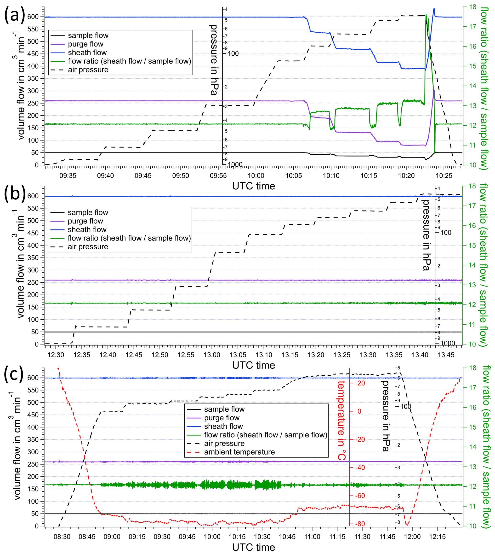
Figure A1 Time series of the UHSAS-A internal flow measurements (sample flow, sheath flow, and purge flow), the ratio between sheath and sample flow, and the air pressure during low-pressure chamber tests with the original pump system of the UHSAS-A (a) and with the new integrated pump system (b). Panel (c) shows the time series for the StratoClim 2017 flight KTM4 (with the new pump system), also including the ambient static air temperature.

Figure A2 Sample flow characterization measurements as a function of pressure.

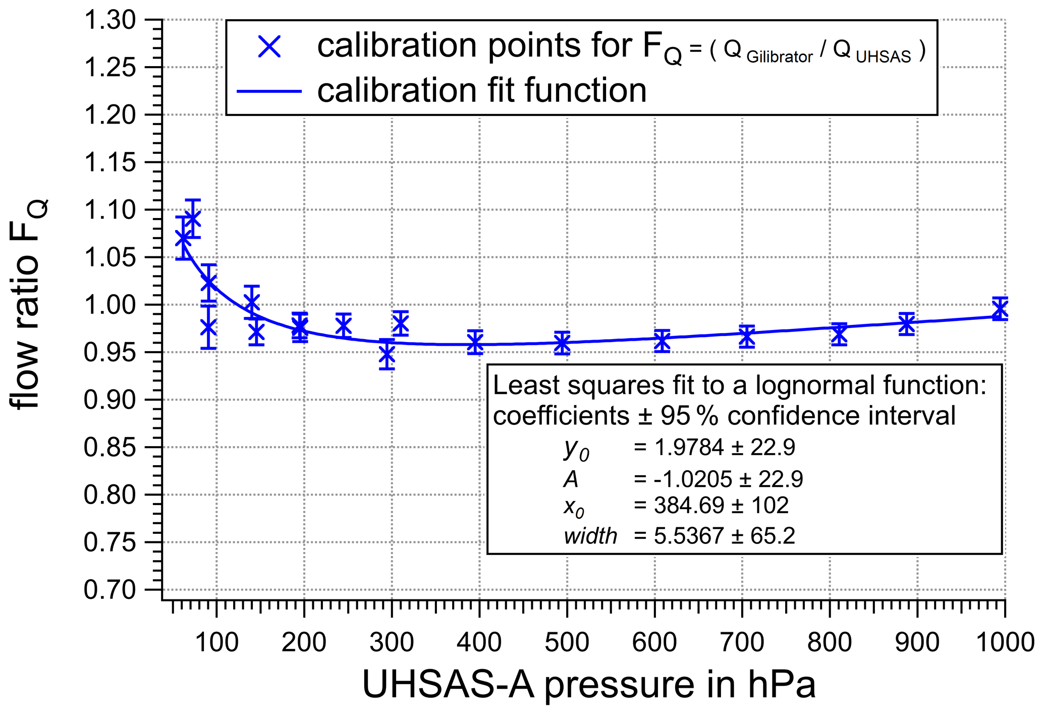
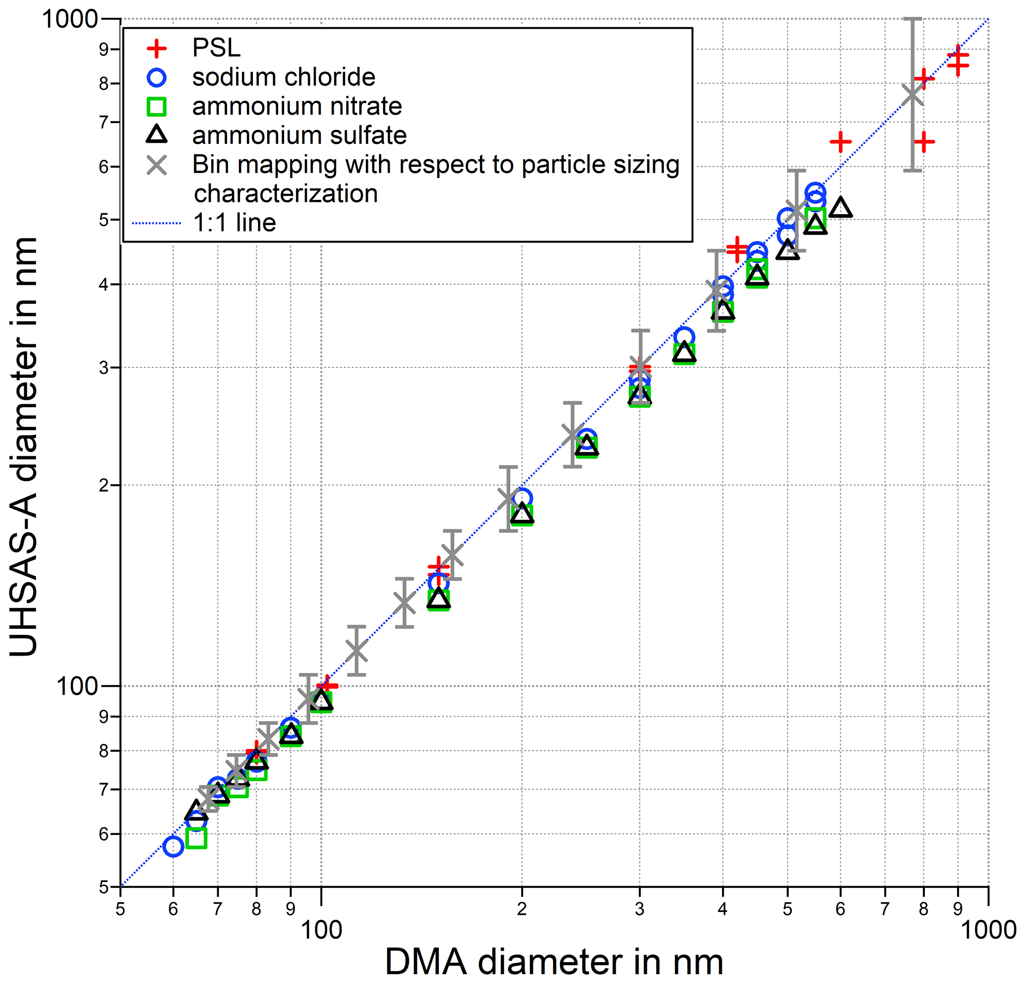
Figure A3 Characterization measurements for the particle sizing of the UHSAS-A: main particle mode diameter of the size distribution measured by the UHSAS-A (using all 99 available size bins) compared with the particle diameter selected by a DMA for different particle species. The gray bars represent the bin mapping used after post-processing.

Figure A2 shows the results of the sample flow characterization measurements as a function of pressure. For these measurements, the UHSAS-A was located in the low-pressure chamber and directly connected through a chamber outlet via a high-precision needle valve with a reference flow meter (Gilibrator-2, SENSIDYNE) located outside of the chamber. For each calibration point, the needle valve was closed a little more. After the sample flow (regulated to 50 cm³ min⁻¹) of the UHSAS-A (Q_UHSAS) and the pressure measured at the UHSAS-A optical measurement cell were stable, the flow measurements with the Gilibrator were done for the respective calibration point. The results of these reference measurements were converted to the pressure conditions measured by the UHSAS-A inside the low-pressure chamber (Q_Gilibrator), making the idealized assumption that the temperature of the air inside the UHSAS-A flow system was equal to the temperature in the laboratory. The ratio $F_Q=Q_{\text{Gilibrator}}/Q_{\text{UHSAS}}$ as a function of the pressure measured in the UHSAS-A optical measurement cell is shown in Fig. A2. The vertical bars represent the results of the error propagation calculated on the basis of the individual uncertainties of the measurements from the flow and pressure meters.

$$\begin{array}{ll}{\displaystyle }{Q}_{\text{UHSAS\_cali}}& {\displaystyle }=Q_{\text{UHSAS}}\\ \text{(A1)}& {\displaystyle }& {\displaystyle }\cdot \left[y_{\text{0}}+A\text{exp}\left\{-{\left({\displaystyle \frac{\text{ln}\left(\frac{p_{\text{UHSAS}}}{x_{\mathrm{0}}}\right)}{\text{width}}}\right)}^{\mathrm{2}}\right\}\right]\end{array}$$

The calculated lognormal fit function (coefficients reported in Fig. A2) and Eq. (A1) allow for a calibration of the sample flow measurement (Q_UHSAS) as a function of pressure (p_UHSAS) to Q_{UHSAS_cali}.

A2 Particle sizing

As the UHSAS-A measures the particle size based on the intensity of the laser light scattered by the individual aerosol particles, the particle size determination is also dependent on the species of the aerosol particle. As described in Sect. 3.1, the calibration of the UHSAS-A was performed with PSL particle standards that were also selected according to size by a DMA (TSI 3080 with TSI 3081), whereas we want to measure complex mixtures of different aerosol particle species in the free atmosphere. In order to confirm the previous size calibration with PSL particle standards, measurements with PSL particles of different sizes were carried out. Subsequently, as already shown by Cai et al. (2008) for the laboratory version of the UHSAS, measurements with sodium chloride, ammonium nitrate, and ammonium sulfate were carried out.

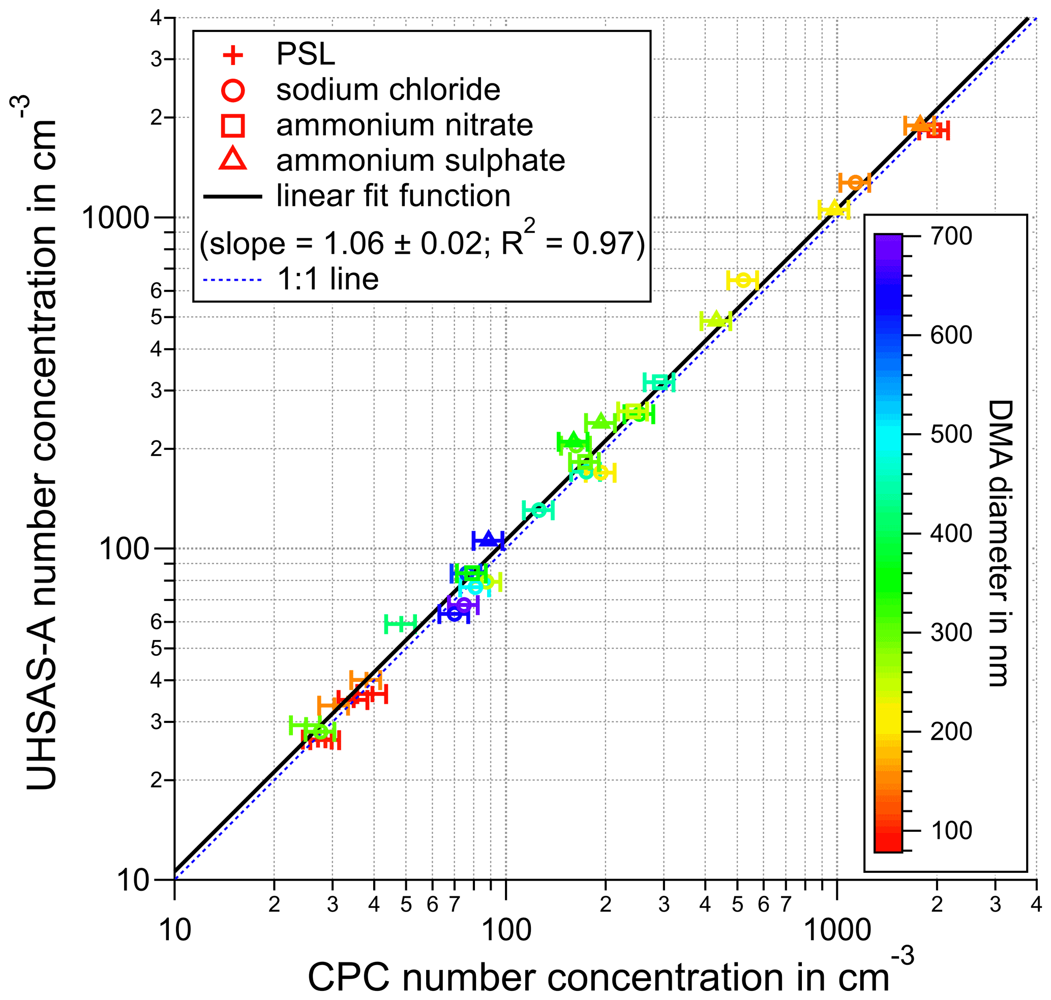
Figure A4 Characterization measurements of the counting efficiency of the UHSAS-A: comparison of the particle number concentrations measured by the UHSAS-A and the TSI CPC 3025A reference for different particle species and particle sizes (color coded).

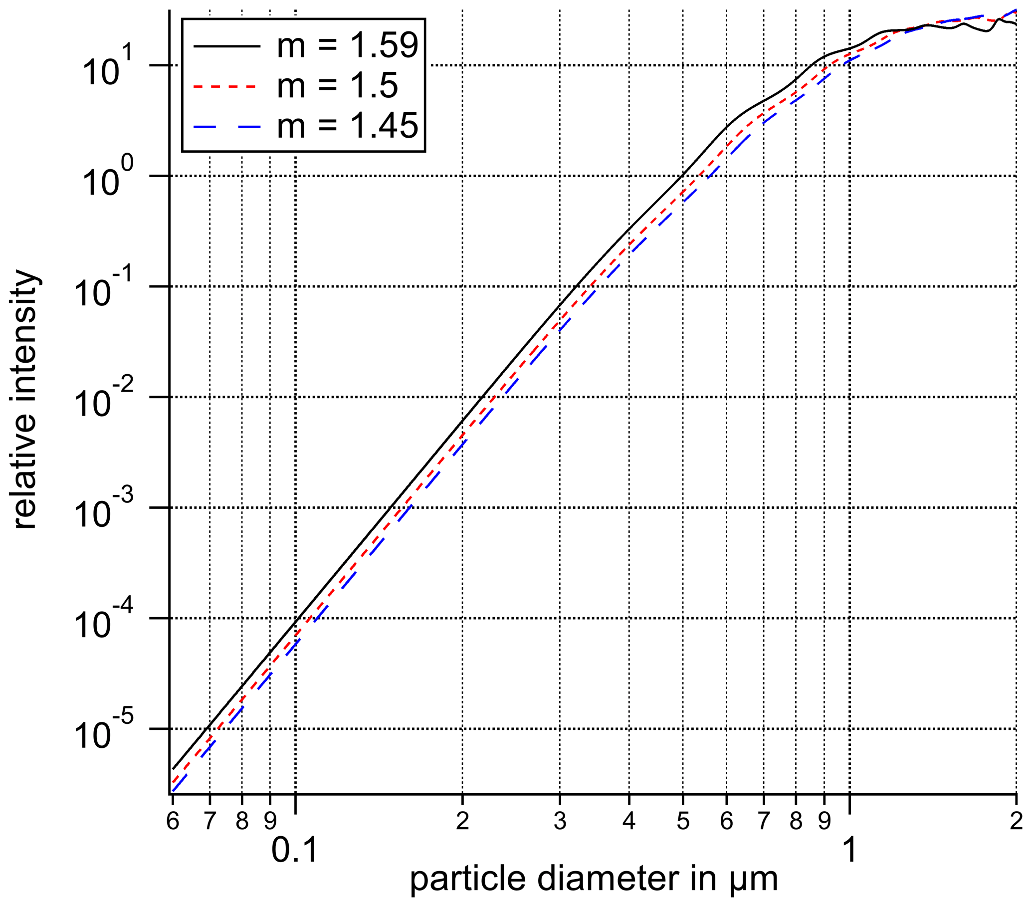
Figure A5 Relative intensity at the detector of UHSAS-A calculated for the refractive index of PSL particles (m=1.59), ATAL aerosol particles (m=1.5), and stratospheric aerosol particles (m=1.45).

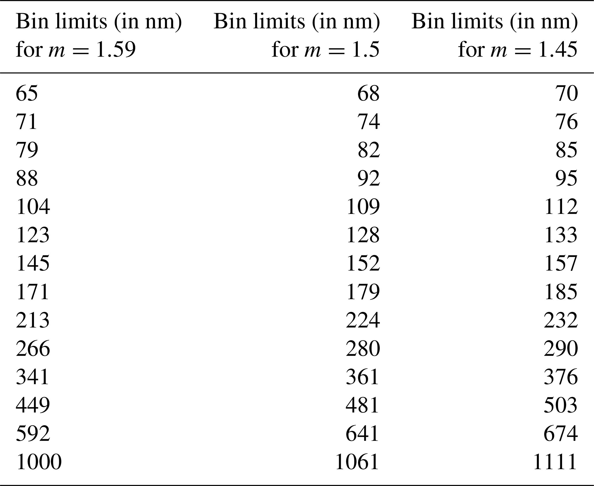
Table A1 UHSAS-A bin limits for the calibration with PSL particles (refractive index m=1.59), recalibrated for refractive indices of 1.5 and 1.45.

For each particle size and species, size distributions averaged over several minutes were generated. The DMA allowed the selection of particles with diameters of up to 1 µm. Therefore, measurements at the upper end of the UHSAS-A size range could be performed. For particle diameters larger than 600 nm, however, only high concentrations of preselected PSL standards could provide a sufficient number of particles to the UHSAS-A in order to allow for measurements with low variability due to counting statistics. For sodium chloride, ammonium nitrate, and ammonium sulfate, the aerosol generator used was not able to generate enough particles of these sizes. Hence, after selection by the DMA and possible line losses, only an insufficient number of these large particles could reach the detection cell of the UHSAS-A. Figure A3 shows the results of these measurements, comparing the main particle mode diameter of the size distribution measured by the UHSAS-A (using all 99 available size bins) with the particle (electrical mobility) diameter selected by a DMA for different particle species. The gray bars represent the bin mapping used after post-processing. These bin limits were selected as a compromise between the size resolution and a reasonable averaging time at low number concentrations, as well as the ability of the UHSAS-A to resolve the signal response (most relevant for particles with a diameter >600 nm).

For each particle species, a linear regression was calculated. Considering the slopes of the linear regression function for PSL particles with a value of 0.99, there is a discrepancy of only 1 % between the DMA set mobility diameter and the measurement from the UHSAS-A. Comparing the slopes of the linear regressions of sodium chloride, ammonium nitrate, and ammonium sulfate with those reported by Cai et al. (2008), for results obtained with the laboratory version of the UHSAS, the particle size measurements of both instruments show a similar dependence on the particle species. For example, the slopes of sodium chloride at 0.96±0.01 and ammonium nitrate at 0.92±0.01 in Cai et al. (2008) agree, within the confidence interval, with the slopes of 0.97±0.01 for sodium chloride and 0.91±0.01 for ammonium nitrate determined here. However, ammonium sulfate, with a slope of 0.89±0.01 for the UHSAS-A, shows a much larger deviation from the DMA diameter than that reported by Cai et al. (2008) with $\mathrm{0.96}\pm \mathrm{0.01}.$ This could, for example, be due to insufficient drying of the particles in the diffusion dryer. In order to exclude this, Cai et al. (2008) also measured the relative humidity in their system and reported it as RH <15 %. As the relative humidity was not measured in the experimental setup used here, an influence of residual moisture on the measurement cannot be excluded.

Based on limited laboratory studies, Kupc et al. (2018) reported that black carbon particles might incandesce and vaporize due to the particles' absorption of energy from the UHSAS-A detector laser (optical cavity laser power of ∼1 kW cm⁻² at 1054 nm). This effect and the complex refractive index of black carbon would alter the sizing of black carbon particles significantly. While particles might be undersized because of the complex refractive index, the incandescing of black carbon particles could potentially result in an oversizing or an undersizing of these particles.

A3 Counting efficiency

To characterize the counting efficiency of the UHSAS-A, the aerosol line between the DMA and the UHSAS-A (as described in Appendix A2) was split, and one line was connected to a condensation particle counter (CPC, TSI 3025A) as a reference. In total, 32 measuring series with PSL, sodium chloride, ammonium nitrate, and ammonium sulfate particles of different sizes (selected with a DMA) and number concentrations (between 30 and 2000 cm⁻³), each averaged over 100 s, were conducted. The results of these measurements are shown in Fig. A4, with the electrical mobility diameter set at the DMA color coded. The correlation coefficient R²=0.97 confirms the linear correlation between the particle number concentrations measured by the UHSAS-A and the CPC over 3 orders of magnitude. The slope of the linear fit function was calculated to be 1.06, while the intercept was forced to be 0 (after successful zero filter tests with both instruments). A dependence on the particle size is not visible in the particle size range used here. Therefore, the accuracy of the particle number concentration measured by the UHSAS-A under laboratory conditions was estimated to be 10 %, limited by the accuracy reported for the reference instrument (CPC).

A4 Recalibration of the UHSAS-A bin limits

The UHSAS-A was calibrated with PSL standard particles, as described in Sect. 3.1. These particles have a refractive index of m=1.59 (Heim et al., 2008). For the aerosol backscatter calculations (Sect. 6.1), the bin limits were recalibrated for a refractive index of m=1.45 and m=1.5 (see Table A1). This was done by calculating the response of the UHSAS-A (laser wavelength of 1054 nm; collection angle of 22^∘ to 158^∘, as reported by Cai et al., 2008) using custom software written by Vetter (2004), which is based on the algorithms described in Bohren and Huffmann (2008). Figure A5 shows the relative intensity at the detector calculated for these three refractive indices.

Appendix B: Sensitivity of the backscatter calculation to particle size and refractive index

To estimate the influence of the uncertainties from the aerosol particle size distribution measurements on the aerosol backscatter calculations, a sensitivity study was performed as follows: the aerosol backscatter coefficient was calculated for a set of 42 size distributions (each averaged over a 100 s interval) from StratoClim 2017 flight KTM3 using a refractive index of m=1.5. The calculations were then repeated after the bin limits of the size distributions were shifted by 10 % to larger values and once more after the values of the bin limits were made 10 % smaller than the reference case. As a next step, the backscatter calculations were done using the original bin limits changing the refractive index to 1.45 and once more to 1.55. The results of these calculations (Fig. B1) do not vary by more than 50 % from the reference case. This also agrees with the variations of the backscatter calculations reported in Cairo et al. (2011).

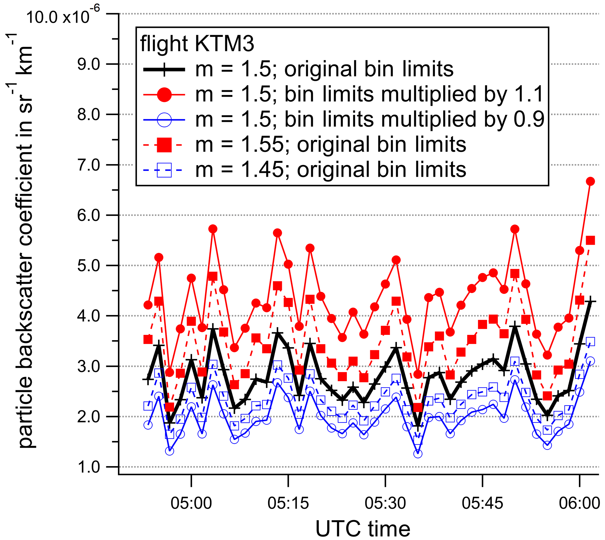
Figure B1 Sensitivity test of the aerosol backscatter coefficient calculation for different refractive indices (m=1.45, m=1.5, and m=1.55) and shifts of the bin limits of the aerosol size distribution by ±10 %.

Appendix C: BR variability in the remote sensing measurements during StratoClim 2017

The standard deviation for the backscatter ratio profile calculated based on the aerosol particle size distributions measured during StratoClim 2017 is shown in Fig. 7. Figure C1 additionally reports the standard deviation for the backscatter ratio profiles measured by CALIOP, MAS, and MAL as horizontal bars.

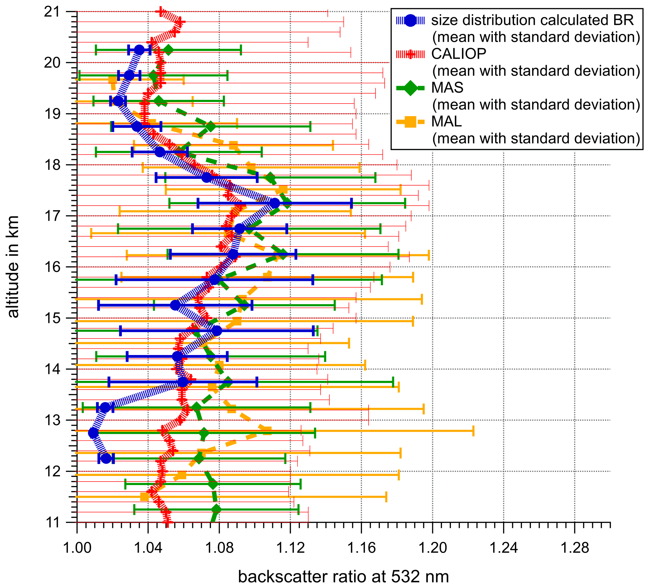
Figure C1 Vertical profile of the backscatter ratio at a 532 nm wavelength. The mean profile (blue line) and standard deviation (blue bars) of the calculated BR based on the aerosol size distributions measured during the 2017 StratoClim measurement campaign are shown. The mean profiles (with the standard deviation as horizontal bars) of the backscatter ratio at a 532 nm wavelength measured by CALIOP, MAS, and MAL are plotted in red, green, and orange, respectively.